fundamentals of digital audio processing - cscsmc.dei.unipd.it/education/algo4smc_ch1.pdf ·...
TRANSCRIPT

Chapter 1
Fundamentals of digital audio processing
Federico Avanzini and Giovanni De Poli
Copyright c© 2005-2012 Federico Avanzini and Giovanni De Poliexcept for paragraphs labeled as adapted from <reference>
This book is licensed under the CreativeCommons Attribution-NonCommercial-ShareAlike 3.0 license.To view a copy of this license, visit http://creativecommons.org/licenses/by-nc-sa/3.0/, or send a letter to
Creative Commons, 171 2nd Street, Suite 300, San Francisco, California, 94105, USA.
1.1 Introduction
The purpose of this chapter is to provide the reader with fundamental concepts of digital signal pro-cessing, which will be used extensively in the reminder of the book. Since the focus is on audiosignals, all the examples deal with sound. Those who are already fluent in DSP may skip this chapter.
1.2 Discrete-time signals and systems
1.2.1 Discrete-time signals
Signals play an important role in our daily life. Examples of signals that we encounter frequently arespeech, music, picture and video signals. A signal is a function of independent variables such as time,distance, position, temperature and pressure. For examples, speech and music signals represent airpressure as a function of time at a point in space.
Most signals we encounter are generated by natural means. However, a signal can also generatedsynthetically or by computer simulation. In this chapter we will focus our attention on a particularyclass of signals: The so called discrete-time signals. This class of signals is the most important wayto describe/model the sound signals with the aid of the computer.
1.2.1.1 Main definitions
We define a signal x as a function x : D → C from a domainD to a codomain C. For our purposes thedomain D represents a time variable, although it may have different meanings (e.g. it may represent

1-2 Algorithms for Sound and Music Computing [v.March 13, 2012]
0 0.1 0.2 0.3 0.4 0.5 0.6 0.7 0.80.5
1
1.5
2
2.5
3
3.5
t (s)
ampl
itude
(m
V)
(a)
0 0.1 0.2 0.3 0.4 0.5 0.6 0.7 0.81
2
3
4
5
6
7
8
t (s)
disc
rete
am
plitu
de (
mV
)
(b)
0 0.1 0.2 0.3 0.4 0.5 0.6 0.7 0.80.5
1
1.5
2
2.5
3
3.5
t (s)
ampl
itude
(m
V)
(c)
0 0.1 0.2 0.3 0.4 0.5 0.6 0.7 0.81
2
3
4
5
6
7
8
t (s)
disc
rete
am
plitu
de (
mV
)
(d)
Figure 1.1: (a) Analog, (b) quantized-analog, (c) discrete-time, and (d) numerical signals.
spatial variables). A signal can be classified based on the nature of D and C. In particular these setscan be countable or non-countable. Moreover, C may be a subset of R or C, i.e. the signal x may beeither a real-valued or a complex-valued function.
When D = R we talk of continuous-time signals x(t), where t ∈ R, while when D = Z we talkof discrete-time signals x[n]. In this latter case n ∈ Z identifies discrete time instants tn: the mostcommon and important example is when tn = nTs, with Ts is a fixed quantity. In many practicalapplications a discrete-time signal xd is obtained by periodically sampling a continuous-time signalxc, as follows:
xd[n] = xc(nTs) −∞ < n <∞, (1.1)
The quantity Ts is called sampling period, measured in s. Its its reciprocal is the sampling frequency,measured in Hz, and is usually denoted as Fs = 1/Ts. Note also the use of square brackets in thenotation for a discrete-time signal x[n], which avoids ambiguity with the notation x(t) used for acontinuous-time signal.
When C = R we talk of continuous-amplitude signals, while when C = Z we talk of discrete-amplitude signals. Typically the range of a discrete-amplitude signal is a finite set of M valuesxkMk=1, and the most common example is that of a uniformly quantized signal with xk = kq (whereq is called quantization step).
By combining the above options we obtains the following classes of signals, depicted in Fig. 1.1:
1. D = R, C = R: analog signal.
2. D = R, C = Z: quantized analog signal.
3. D = Z, C = R: sequence, or sampled signal.
This book is licensed under the CreativeCommons Attribution-NonCommercial-ShareAlike 3.0 license,c©2005-2012 by the authors except for paragraphs labeled as adapted from <reference>

Chapter 1. Fundamentals of digital audio processing 1-3
4. D = Z, C = Z: numerical, or digital, signal. This is the type of signal that can be processedwith the aid of the computer.
In these sections we will focus on discrete-time signals, regardless of whether they are quantized ornot. We will equivalently use the terms discrete-time signal and sequence. We will always refer to asingle value x[n] as the n-th sample of the sequence x, regardless of whether the sequence has beenobtained by sampling a continuous-time signal or not.
1.2.1.2 Basic sequences and operations
Sequences are manipulated through various basic operations. The product and sum between twosequences are simply defined as the sample-by-sample product sequence and sum sequence, respec-tively. Multiplication by a constant is defined as the sequence obtained by multiplying each sampleby that constant. Another important operation is time shifting or translation: we say that a sequencey[n] is a shifted version of x[n] if
y[n] = x[n− n0], (1.2)
with n0 ∈ Z. For n0 > 0 this is a delaying operation while for n0 < 0 it is an advancing operation.Several basic sequences are relevant in discussing discrete-time signals and systems. The simplest
and the most useful sequence is the unit sample sequence δ[n], often referred to as unit impulse orsimply impulse:
δ[n] =
1, n = 0,
0, n 6= 0.(1.3)
The unit impulse is also the simplest example of a finite-legth sequence, defined as a sequence thatis zero except for a finite interval n1 ≤ n ≤ n2. One trivial but fundamental property of the δ[n]sequence is that any sequence can be represented as a linear combination of delayed impulses:
x[n] =∞∑
k=−∞x[k]δ[n− k]. (1.4)
The unit step sequence is denoted by u[n] and is defined as
u[n] =
1, n ≥ 0,
0, n < 0.(1.5)
The unit step is the simplest example of a right-sided sequence, defined as a sequence that is zeroexcept for a right-infinite interval n1 ≤ n < +∞. Similarly, left-sided sequences are defined as asequences that are zero except for a left-infinite interval −∞ < n ≤ n1.
The unit step is related to the impulse by the following equalities:
u[n] =∞∑
k=0
δ[n− k] =n∑
k=−∞δ[k]. (1.6)
Conversely, the impulse can be written as the first backward difference of the unit step:
δ[n] = u[n]− u[n− 1]. (1.7)
The general form of the real sinusoidal sequence with constant amplitude is
x[n] = A cos(ω0n + φ), −∞ < n <∞, (1.8)
This book is licensed under the CreativeCommons Attribution-NonCommercial-ShareAlike 3.0 license,c©2005-2012 by the authors except for paragraphs labeled as adapted from <reference>

1-4 Algorithms for Sound and Music Computing [v.March 13, 2012]
where A, ω0 and φ are real numbers. By analogy with continuous-time functions, ω0 is called angularfrequency of the sinusoid, and φ is called the phase. Note however that, since n is dimensionless, thedimension of ω0 is radians. Very often we will say that the dimension of n is “samples” and thereforewe will specify the units of ω0 to be radians/sample. If x[n] has been sampled from a continuous-timesinusoid with a given sampling rate Fs, we will also use the term normalized angular frequency, sincein this case ω0 is the continuous-time angular frequency normalized with respect to Fs.
Another relevant numerical signal is constructed as the sequence of powers of a real or complexnumber α. Such sequences are termed exponential sequences and their general form is
x[n] = Aαn, −∞ < n <∞, (1.9)
where A and α are real or complex constant. When α is complex, x[n] has real and imaginary partsthat are exponentially weighted sinusoid. Specifically, if α = |α|ejω0 and A = |A|ejφ, then x[n] canbe expressed as
x[n] = |A | |α |n · ej(ω0n+φ) = |A | |α |n · (cos(ω0n + φ) + j sin(ω0n + φ)) . (1.10)
Therefore x[n] can be expressed as x[n] = xRe[n] + jxIm[n], with xRe[n] = |A | |α |n cos(ω0n+φ)and xIm[n] = |A | |α |n sin(ω0n + φ). These sequences oscillate with an exponentially growingmagnitude if |α | > 1, or with an exponentially decaying magnitude if |α | < 1. When |α | = 1,the sequences xRe[n] and xIm[n] are real sinusoidal sequences with constant amplitude and x[n] isreferred to as a the complex exponential sequence.
An important property of real sinusoidal and complex exponential sequences is that substitutingthe frequency ω0 with ω0 + 2πk (with k integer) results in sequences that are indistinguishable fromeach other. This can be easily verified and is ultimately due to the fact that n is integer. We will seethe implications of this property when discussing the Sampling Theorem in Sec. 1.4.1, for now wewill implicitly assume that ω0 varies in an interval of length 2π, e.g. (−π, π], or [0, 2π).
Real sinusoidal sequences and complex exponential sequences are also examples of a periodicsequence: we define a sequence to be periodic with period N ∈ N if it satisfies the equality x[n] =x[n + kN ], for −∞ < n < ∞, and for any k ∈ Z. The fundamental period N0 of a periodic signalis the smallest value of N for which this equality holds. In the case of Eq. (1.8) the condition ofperiodicity implies that ω0N0 = 2πk. If k = 1 satisfies this equality we can say that the sinusoidalsequence is periodic with period N0 = 2π/ω0, but this is not always true: the period may be longeror, depending on the value of ω0, the sequence may not be periodic at all.
1.2.1.3 Measures of discrete-time signals
We now define a set of useful metrics and measures of signals, and focus exclusively on digital signals.The first important metrics is energy: in physics, energy is the ability to do work and is measured inN·m or Kg·m2/s2, while in digital signal processing physical units are typically discarded and signalsare renormalized whenever convenient. The total energy of a sequence x[n] is then defined as:
Ex =∞∑
n=−∞|x[n]|2. (1.11)
Note that an infinite-length sequence with finite sample values may or not have finite energy. The rateof transporting energy is known as power. The average power of a sequence x[n] is then defined asthe average energy per sample:
Px =ExN
=1N
N−1∑
n=0
|x[n]|2. (1.12)
This book is licensed under the CreativeCommons Attribution-NonCommercial-ShareAlike 3.0 license,c©2005-2012 by the authors except for paragraphs labeled as adapted from <reference>

Chapter 1. Fundamentals of digital audio processing 1-5
Another common description of a signal is its root mean square (RMS) level. The RMS level of asignal x[n] is simply
√Px. In practice, especially in audio, the RMS level is typically computedafter subtracting out any nonzero mean value, and is typically used to characterize periodic sequencesin which Px is computed over a cycle of oscillation: as an example, the RMS level of a sinusoidalsequence x[n] = A cos(ω0n + φ) is A/
√2.
In the case of sound signals, x[n] will typically represent a sampled acoustic pressure signal. Asa pressure wave travels in a medium (e.g., air), the RMS power is distributed all along the surface ofthe wavefront so that the appropriate measure of the strength of the wave is power per unit area ofwavefront, also known as intensity.
Intensity is still proportional to the RMS level of the acoustic pressure, and relates to the soundlevel perceived by a listener. However, the usual definition of sound pressure level (SPL) does notdirectly use intensity. Insted the SPL of a pressure signal is measured in decibels (dB), and is definedas
SPL = 10 log10(I/I0) (dB), (1.13)
where I and I0 are the RMS intensity of the signal and a reference intensity, respectively. In particular,in an absolute dB scale I0 is chosen to be the smallest sound intensity that can be heard (more on thisin Chapter Auditory based processing). The function of the dB scale is to transform ratios into differences: ifI2 is twice I1, then SPL2 − SPL1 = 3 dB, no matter what the actual value of I1 might be.1
Because sound intensity is proportional to the square of the RMS pressure, it is easy to expresslevel differences in terms of pressure ratios:
SPL2 − SPL1 = 10 log10(p22/p2
1) = 20 log10(p2/p1) (dB). (1.14)
Therefore, depending on the physical quantity which is being used the prefactor 20 or 10 may beemployed in a decibel calculation. To resolve the uncertainty of which is the correct one, note thatthere are two kinds of quantities for which a dB scale is appropriate: “energy-like” quantities and “dy-namical” quantities. An energy-like quantity is real and never negative: examples of such quantitiesare acoustical energy, intensity or power, electrical energy or power, optical luminance, etc., and theappropriate prefactor for these quantities in a dB scale is 10. Dynamical quantities may be positive ornegative, or even complex in some representations: examples of such quantities are mechanical dis-placement or velocity, acoustical pressure, velocity or volume velocity, electrical voltage or current,etc., and the appropriate prefactor for these quantities in a dB scale is 20 (since they have the propertythat their squares are energy-like quantities).
1.2.1.4 Random signals
1.2.2 Discrete-time systems
Signal processing systems can be classified along the same lines used in Sec. 1.2 to classify signals.Here we are interested in discrete-time systems, that act on sequences and produce sequences asoutput.
1This is a special case of the Weber-Fechner law, which attempts to describe the relationship between the physicalmagnitudes of stimuli and the perceived intensity of the stimuli: the law states that this relation is logaritmic: if a stimulusvaries as a geometric progression (i.e. multiplied by a fixed factor), the corresponding perception is altered in an arithmeticprogression (i.e. in additive constant amounts).
This book is licensed under the CreativeCommons Attribution-NonCommercial-ShareAlike 3.0 license,c©2005-2012 by the authors except for paragraphs labeled as adapted from <reference>
1-6 Algorithms for Sound and Music Computing [v.March 13, 2012]
T . y[n]x[n]
(a)
T1x[n]
T1y[n]...
timesn
Tn0
0
(b)
M2
M1
−121(M +M +1)
...T T
...
times
T1T1
times
x[n]
y[n]
TMA
−1 −1
(c)
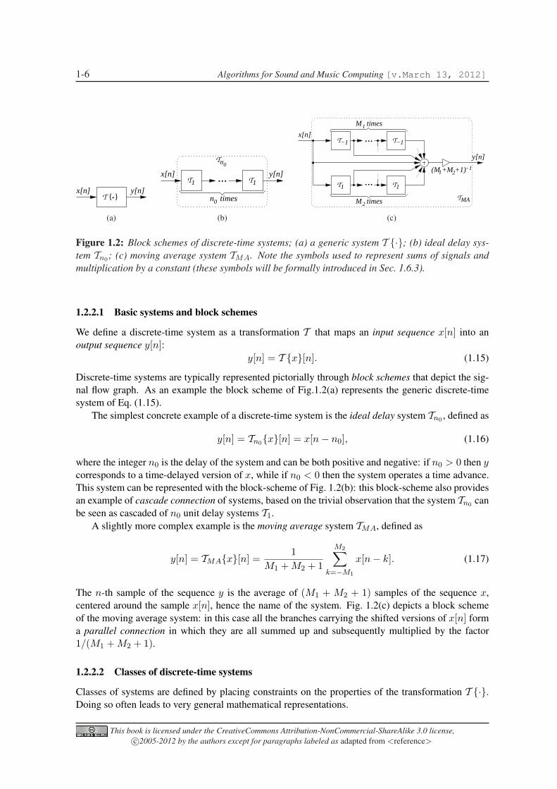
Figure 1.2: Block schemes of discrete-time systems; (a) a generic system T ·; (b) ideal delay sys-tem Tn0; (c) moving average system TMA. Note the symbols used to represent sums of signals andmultiplication by a constant (these symbols will be formally introduced in Sec. 1.6.3).
1.2.2.1 Basic systems and block schemes
We define a discrete-time system as a transformation T that maps an input sequence x[n] into anoutput sequence y[n]:
y[n] = T x[n]. (1.15)
Discrete-time systems are typically represented pictorially through block schemes that depict the sig-nal flow graph. As an example the block scheme of Fig.1.2(a) represents the generic discrete-timesystem of Eq. (1.15).
The simplest concrete example of a discrete-time system is the ideal delay system Tn0 , defined as
y[n] = Tn0x[n] = x[n− n0], (1.16)
where the integer n0 is the delay of the system and can be both positive and negative: if n0 > 0 then ycorresponds to a time-delayed version of x, while if n0 < 0 then the system operates a time advance.This system can be represented with the block-scheme of Fig. 1.2(b): this block-scheme also providesan example of cascade connection of systems, based on the trivial observation that the system Tn0 canbe seen as cascaded of n0 unit delay systems T1.
A slightly more complex example is the moving average system TMA, defined as
y[n] = TMAx[n] =1
M1 + M2 + 1
M2∑
k=−M1
x[n− k]. (1.17)
The n-th sample of the sequence y is the average of (M1 + M2 + 1) samples of the sequence x,centered around the sample x[n], hence the name of the system. Fig. 1.2(c) depicts a block schemeof the moving average system: in this case all the branches carrying the shifted versions of x[n] forma parallel connection in which they are all summed up and subsequently multiplied by the factor1/(M1 + M2 + 1).
1.2.2.2 Classes of discrete-time systems
Classes of systems are defined by placing constraints on the properties of the transformation T ·.Doing so often leads to very general mathematical representations.
This book is licensed under the CreativeCommons Attribution-NonCommercial-ShareAlike 3.0 license,c©2005-2012 by the authors except for paragraphs labeled as adapted from <reference>

Chapter 1. Fundamentals of digital audio processing 1-7
We define a system to be memoryless if the output sequence y[n] at every value of n dependsonly on the value of the input sequence x[n] at the same value of n. As an example, the systemy[n] = sin(x[n]) is a memoryless system. On the other hand, the ideal delay system and the movingaverage system described in the previous section are not memoryless: these systems are referred to ashaving memory, since they must “remember” past (or even future) values of the sequence x in orderto compute the “present” output y[n].
We define a system to be linear if it satisfies the principle of superposition. If y1[n], y2[n] are theresponses of a system T to the inputs x1[n], x2[n], respectively, then T is linear if and only if
T a1x1 + a2x2[n] = a1T x1[n] + a2T x2[n], (1.18)
for any pair of arbitrary constants a1 and a2. Equivalently we say that a linear system possesses anadditive property and a scaling property. As an example, the ideal delay system and the moving aver-age system described in the previous section are linear systems. On the other hand, the memorylesssystem y[n] = sin(x[n]) discussed above is clearly non-linear.
We define a system to be time-invariant (or shift-invariant) if a time shift of the input sequencecauses a corresponding shift in the output sequence. Specifically, let y = T x. Then T is time-invariant if and only if
T Tn0x [n] = y[n− n0] ∀n0, (1.19)
where Tn0 is the ideal delay system defined previously. This relation between the input and the outputmust hold for any arbitrary input sequence x and its corresponding output. All the systems thatwe have examined so far are time-invariant. On the other hand, an example of non-time-invariantsystem is y[n] = x[Mn] (with M ∈ N). This system creates y by selecting one every M samplesof x. One can easily see that T Tn0x [n] = x[Mn − n0], which is in general different fromy[n− n0] = x[M(n− n0)].
We define a system to be causal if for every choice of n0 the output sequence sample y[n0]depends only on the input sequence samples x[n] with n ≤ n0. This implies that, if y1[n], y2[n] arethe responses of a causal system to the inputs x1[n], x2[n], respectively, then
x1[n] = x2[n] ∀n < n0 ⇒ y1[n] = y2[n] ∀n < n0. (1.20)
The moving average system discussed in the previous section is an example of a non-causal systems,since it needs to know M1 “future” values of the input sequence in order to compute the current valuey[n]. Apart from this, all the systems that we have examined so far are causal.
We define a system to be stable if and only if every bounded input sequence produces a boundedoutput sequence. A sequence x[n] is said to be bounded if there exist a positive constant Bx such that
|x[n] | ≤ Bx ∀n. (1.21)
Stability then requires that for such an input sequence there exists a positive constant By such that| y[n] | ≤ By ∀n. This notion of stability is often referred to as bounded-input bounded-output (BIBO)stability. All the systems that we have examined so far are BIBO-stable. On the other hand, anexample of unstable system is y[n] =
∑nk=−∞ x[k]. This is called the accumulator system, since y[n]
accumulates the sum of all past values of x. In order to see that the accumulator system is not stableit is sufficient to verify that y[n] is not bounded when x[n] is the step sequence.
This book is licensed under the CreativeCommons Attribution-NonCommercial-ShareAlike 3.0 license,c©2005-2012 by the authors except for paragraphs labeled as adapted from <reference>

1-8 Algorithms for Sound and Music Computing [v.March 13, 2012]
1.2.3 Linear Time-Invariant Systems
Linear-time invariant (LTI) are a particularly relevant class of systems. A LTI system is any systemthat is both linear and time-invariant according to the definitions given in the previous section. As wewill see in this section, LTI systems are mathematically easy to analyze and to characterize.
1.2.3.1 Impulse response and convolution
Let T be a LTI system, y[n] = T x[n] be the output sequence given a generic input x, and h[n] theimpulse response of the system, i.e. h[n] = T δ[n]. Now, recall that every sequence x[n] can berepresented as a linear combination of delayed impulses (see Eq. (1.4)). If we use this representationand exploit the linearity and time-invariance properties, we can write:
y[n] = T
+∞∑
k=−∞x[k]δ[n− k]
=
+∞∑
k=−∞x[k]T δ[n− k] =
+∞∑
k=−∞x[k]h[n− k], (1.22)
where in the first equality we have used the representation (1.4), in the second equality we have usedthe linearity property, and in the last equality we have used the time-invariance property.
Equation (1.22) states that a LTI system can be completely characterized by its impulse responseh[n], since the response to any imput sequence x[n] can be written as
∑∞k=−∞ x[n]h[n−k]. This can
be interpreted as follows: the k-th input sample, seen as a single impulse x[k]δ[n− k], is transformedby the system into the sequence x[k]h[n− k], and for each k these sequences are summed up to formthe overall output sequence y[n].
The sum on the right-hand side of Eq. (1.22) is called convolution sum of the sequences x[n] andh[n], and is usually denoted with the sign ∗. Therefore we have just proved that a LTI system T hasthe property
y[n] = T x[n] = (x ∗ h)[n]. (1.23)
Let us consider again the systems defined in the previous sections: we can find their impulseresponses through the definition, i.e. by computing their response to an ideal impulse δ[n]. For theideal delay system the impulse response is simply a shifted impulse:
hn0 [n] = δ[n− n0]. (1.24)
The impulse response of the moving average system is easily computed as
h[n] =1
M1 + M2 + 1
M2∑
k=−M1
δ[n− k] =
1
M1+M2+1 , −M1 < n < M2,
0, elsewhere.(1.25)
Finally the accumulator system has the following impulse response:
h[n] =n∑
k=−∞δ[k] =
1, n ≥ 0,
0, n < 0.(1.26)
There is a fundamental difference between these impulse responses. The first two responses havea finite number of non-zero samples (1 and M1 + M2 + 1, respectively): systems that possess thisproperty are called finite impulse response (FIR) systems. On the other hand, the impulse response ofthe accumulator has an infinite number of non-zero samples: systems that possess this property arecalled infinite impulse response (IIR) systems.
This book is licensed under the CreativeCommons Attribution-NonCommercial-ShareAlike 3.0 license,c©2005-2012 by the authors except for paragraphs labeled as adapted from <reference>

Chapter 1. Fundamentals of digital audio processing 1-9
h [n]1 h [n]2
h [n]1h [n]2
1 2(h *h )[n]
x[n]
x[n]
x[n] y[n]
y[n]
y[n]
(a)
h [n]1
h [n]2
1 2x[n] y[n]
(h +h )[n]
x[n] y[n]
(b)
Figure 1.3: Properties of LTI system connections, and equivalent systems; (a) cascade, and (b) par-allel connections.
1.2.3.2 Properties of LTI systems
Since the convolution sum of Eq. (1.23) completely characterizes a LTI system, the most relevantproperties of this class of systems can be understood by inspecting properties of the convolution oper-ator. Clearly convolution is linear, otherwise T would not be a linear system, which is by hypothesis.Convolution is also associative:
(x ∗ (h1 ∗ h2)) [n] = ((x ∗ h1) ∗ h2) [n]. (1.27)
Moreover convolution is commutative:
(x ∗ h)[n] =∞∑
k=−∞x[n]h[n− k] =
∞∑m=−∞
x[n−m]h[m] = (h ∗ x)[n], (1.28)
where we have substituted the variable m = n−k in the sum. This property implies that a LTI systemwith input h[n] and impulse response x[n] will have the same ouput of a LTI system with input x[n]and impulse response h[n]. More importantly, associativity and commutativity have implications onthe properties of cascade connections of systems. Consider the block scheme in Fig. 1.3(a) (upperpanel): the output from the first block is x∗h1, therefore the final output is (x∗h1)∗h2, which equalsboth (x ∗ h2) ∗ h1 and x ∗ (h1 ∗ h2). As a result the three block schemes in Fig. 1.3(a) represent threesystems with the same impulse response.
Linearity and commutativity imply that the convolution is distributive over addition. From thedefinition (1.23) it is straightforward to prove that
(x ∗ (h1 + h2)) [n] = (x ∗ h1)[n] + (x ∗ h2)[n]. (1.29)
Distributivity has implications on the properties of parallel connections of systems. Consider theblock scheme in Fig. 1.3(b) (upper panel): the final output is (x ∗ h1) + (x ∗ h2), which equalsx ∗ (h1 + h2). As a result the two block schemes in Fig. 1.3(a) represent two systems with the sameimpulse response.
In the case of a LTI system, the notions of causality and stability given in the previous sections canalso be related to properties of the impulse response. As for causality, it is a straightforward exerciseto show that a LTI system is causal if and only if
h[n] = 0 ∀n < 0. (1.30)
This book is licensed under the CreativeCommons Attribution-NonCommercial-ShareAlike 3.0 license,c©2005-2012 by the authors except for paragraphs labeled as adapted from <reference>

1-10 Algorithms for Sound and Music Computing [v.March 13, 2012]
For this reason, sequences that satisfy the above condition are usually termed causal sequences.As for stability, recall that a system is BIBO-stable if any bounded input produces a bounded
output. The response of a LTI system to a bounde input x[n] ≤ Bx is
| y[n] | =∣∣∣∣∣
+∞∑
k=−∞x[k]h[n− k]
∣∣∣∣∣ ≤+∞∑
k=−∞|x[k] | |h[n− k] | ≤ Bx
+∞∑
k=−∞|h[n− k] | . (1.31)
From this chain of inequalities we find that a sufficient condition for the stability of the system is
+∞∑
k=−∞|h[n− k] | =
+∞∑
k=−∞|h[k] | <∞. (1.32)
One can prove that this is also a necessary condition for stability. Assume that Eq. (1.32) does not holdand define the input x[n] = h∗[−n]/ |h[n] | for h[n] 6= 0 (x = 0 elsewhere): this input is bounded byunity, however one can immediately prove that y[0] =
∑+∞k=−∞ |h[k] | = +∞. In conclusion, a LTI
system is stable if and only if h is absolutely summable, or h ∈ L1(Z). A direct consequence of thisproperty is that FIR systems are always stable, while IIR systems may not be stable.
Using the properties demonstrated in this section, we can look back at the impulse responses ofEqs. (1.24,1.25,1.26), and we can immediately immediately prove whether they are stable and causal.
1.2.3.3 Constant-coefficient difference equations
Consider the following constant-coefficient difference equation:
N∑
k=0
aky[n− k] =M∑
k=0
bkx[n− k]. (1.33)
Question: given a set of values for ak and bk, does this equation define a LTI system? The answeris no, because a given input x[n] does not univocally determine the output y[n]. In fact it is easy tosee that, if x[n], y[n] are two sequences satisfying Eq. (1.33), then the equation is satisfied also by thesequences x[n], y[n] + yh[n], where yh is any sequence that satisfies the homogeneous equation:
N∑
k=0
akyh[n− k] = 0. (1.34)
One could show that yh has the general form yh[n] =∑N
m=1 Amznm, where the zm’s are roots of the
polynomial∑N
k=0 akzk (this can be verified by substituting the general form of yh into Eq. (1.34)).
The situation is very much like that of linear constant-coefficient differential equations in continuous-time: since yh has N undetermined coefficients Am, we must specify N additional constraints in orderfor the equation to admit a unique solution. Typically we set some initial conditions. For Eq. (1.33),an initial condition is a set of N consecutive “initial” samples of y[n]. Suppose that the samplesy[−1], y[−2], . . . y[−N ] have been fixed: then all the infinite remaining samples of y can be recur-sively determined through the recurrence equations
y[n] =
−N∑
k=1
ak
a0y[n− k] +
M∑
m=0
bm
a0x[n−m], n ≥ 0,
−N−1∑
k=0
ak
a0y[n + N − k] +
M∑
m=0
bm
a0x[n + N −m], n ≤ −N − 1.
(1.35)
This book is licensed under the CreativeCommons Attribution-NonCommercial-ShareAlike 3.0 license,c©2005-2012 by the authors except for paragraphs labeled as adapted from <reference>
Chapter 1. Fundamentals of digital audio processing 1-11
x[n]
[n−1]δ
y[n]
y[n−1]
(a)
2(M +1) −1
x[n]Accumulator
y[n]
δ 2[n−M −1]
(b)
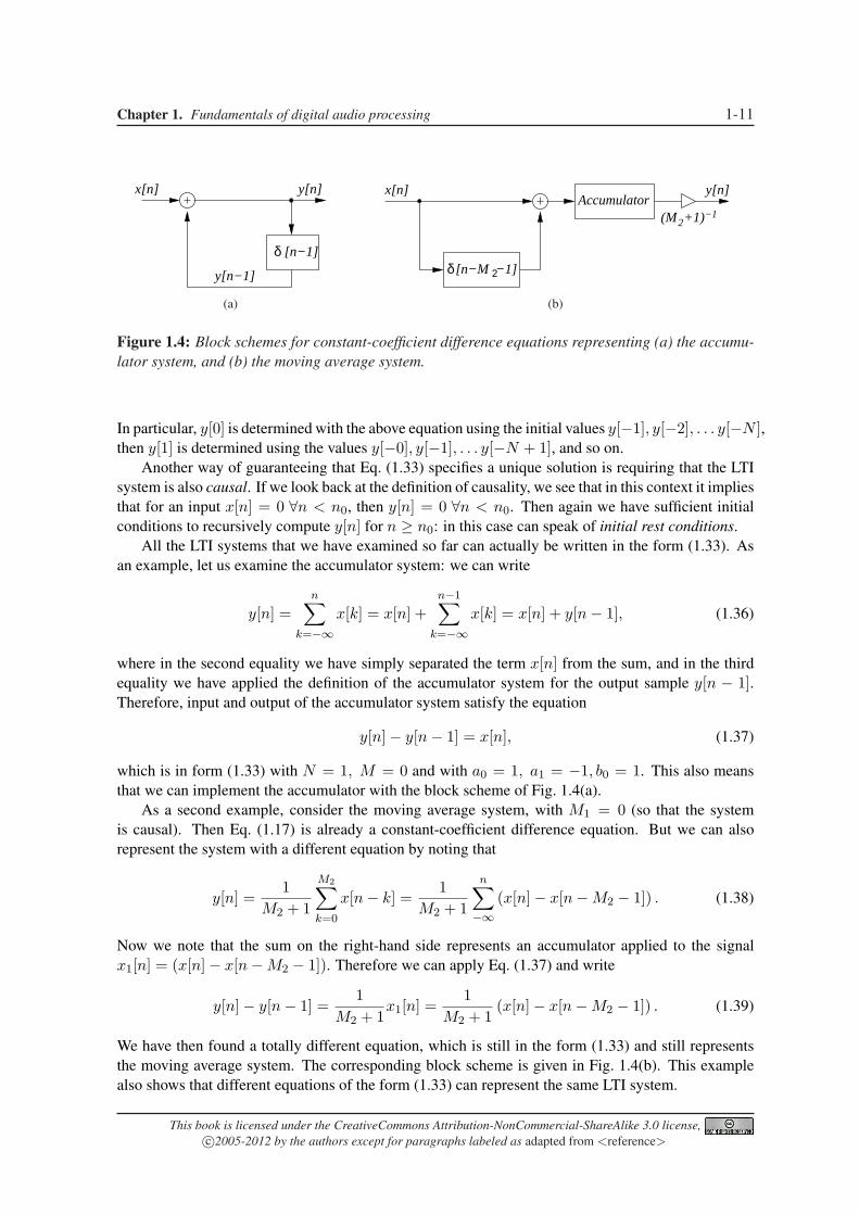
Figure 1.4: Block schemes for constant-coefficient difference equations representing (a) the accumu-lator system, and (b) the moving average system.
In particular, y[0] is determined with the above equation using the initial values y[−1], y[−2], . . . y[−N ],then y[1] is determined using the values y[−0], y[−1], . . . y[−N + 1], and so on.
Another way of guaranteeing that Eq. (1.33) specifies a unique solution is requiring that the LTIsystem is also causal. If we look back at the definition of causality, we see that in this context it impliesthat for an input x[n] = 0 ∀n < n0, then y[n] = 0 ∀n < n0. Then again we have sufficient initialconditions to recursively compute y[n] for n ≥ n0: in this case can speak of initial rest conditions.
All the LTI systems that we have examined so far can actually be written in the form (1.33). Asan example, let us examine the accumulator system: we can write
y[n] =n∑
k=−∞x[k] = x[n] +
n−1∑
k=−∞x[k] = x[n] + y[n− 1], (1.36)
where in the second equality we have simply separated the term x[n] from the sum, and in the thirdequality we have applied the definition of the accumulator system for the output sample y[n − 1].Therefore, input and output of the accumulator system satisfy the equation
y[n]− y[n− 1] = x[n], (1.37)
which is in form (1.33) with N = 1, M = 0 and with a0 = 1, a1 = −1, b0 = 1. This also meansthat we can implement the accumulator with the block scheme of Fig. 1.4(a).
As a second example, consider the moving average system, with M1 = 0 (so that the systemis causal). Then Eq. (1.17) is already a constant-coefficient difference equation. But we can alsorepresent the system with a different equation by noting that
y[n] =1
M2 + 1
M2∑
k=0
x[n− k] =1
M2 + 1
n∑−∞
(x[n]− x[n−M2 − 1]) . (1.38)
Now we note that the sum on the right-hand side represents an accumulator applied to the signalx1[n] = (x[n]− x[n−M2 − 1]). Therefore we can apply Eq. (1.37) and write
y[n]− y[n− 1] =1
M2 + 1x1[n] =
1M2 + 1
(x[n]− x[n−M2 − 1]) . (1.39)
We have then found a totally different equation, which is still in the form (1.33) and still representsthe moving average system. The corresponding block scheme is given in Fig. 1.4(b). This examplealso shows that different equations of the form (1.33) can represent the same LTI system.
This book is licensed under the CreativeCommons Attribution-NonCommercial-ShareAlike 3.0 license,c©2005-2012 by the authors except for paragraphs labeled as adapted from <reference>

1-12 Algorithms for Sound and Music Computing [v.March 13, 2012]
1.3 Signal generators
In this section we describe methods and algorithms used to directly generate a discrete-time signal.Specifically we will examine periodic waveform generators and noise generators, which are bothparticularly relevant in audio applications.
1.3.1 Digital oscillators
Many relevant musical sounds are almost periodic in time. The most direct method for synthesizing aperiodic signal is repeating a single period of the corresponding waveform. An algorithm that imple-ments this method is called oscillator. The simplest algorithm consists in computing the appropriatevalue of the waveform for every sample, assuming that the waveform can be approximately describedthrough a polynomial or rational truncated series. However this is definitely not the most efficientapproach. More efficient algorithms are presented in the remainder of this section.
1.3.1.1 Table lookup oscillator
A very efficient approach is to pre-compute the samples of the waveform, store them in a table whichis usually implemented as a circular buffer, and access them from the table whenever needed. If acopy of one period of the desired waveform is stored in such a wavetable, a periodic waveform can begenerated by cycling over the wavetable with the aid of a circular pointer. When the pointer reachesthe end of the table, it wraps around and points again at the beginning of the table.
Given a table of length L samples, the period T0 of the generated waveform depends on thesampling period Ts at which samples are read. More precisely, the period is given by T0 = LTs,and consequently the fundamental frequency is f0 = Fs/L. This implies that in order to changethe frequency (while maintaing the sample sampling rate), we would need the same waveform to bestored in tables of different lengths.
A better solution is the following. Imagine that a single wavetable is stored, composed of a verylarge number L of equidistant samples of the waveform. Then for a given sampling rate Fs and adesired signal frequency f0, the number of samples to be generated in a single cycle is Fs/f0. Fromthis, we can define the sampling increment (SI), which is the distance in the table between twosamples at subsequent instants. The SI is given by the following equation:
SI =L
Fs/f0=
f0L
Fs. (1.40)
Therefore the SI is proportional to f0. Having defined the sampling increment, samples of the desiredsignal are generated by reading one every SI samples of the table. If the SI is not an integer, the clos-est sample of the table will be chosen (obviously, the largest L, the better the approximation). In thisway, the oscillator resample the table to generate a waveform with different fundamental frequencies.
M-1.1Implement in Matlab a circular look-up from a table of length L and with sampling increment SI.
M-1.1 Solution
phi=mod(phi +SI,L);s=tab[round(phi)];
This book is licensed under the CreativeCommons Attribution-NonCommercial-ShareAlike 3.0 license,c©2005-2012 by the authors except for paragraphs labeled as adapted from <reference>

Chapter 1. Fundamentals of digital audio processing 1-13
where phi is a state variable indicating the reading point in the table, A is a scaling parameter, sis the output signal sample. The function mod(x,y) computes the remainder of the division x/yand is used here to implement circular reading of the table. Notice that phi can be a non integervalue. In order to use it as array index, it has to be truncated, or rounded to the nearest integer (aswe did in the code above). A more accurate output can be obtained by linear interpolation betweenadjacent table values.
1.3.1.2 Recurrent sinusoidal signal generators
Sinusoidal signals can be generated also by recurrent methods. A first method is based on the follow-ing equation:
y[n + 1] = 2 cos(ω0)y[n]− y[n− 1] (1.41)
where ω0 = 2πf0/Fs is the normalized angular frequency of the sinusoid. Then one can prove thatgiven the initial values y[0] = cosφ and y[−1] = cos(φ− ω0) the generator produces the sequence
y[n] = cos(ω0 + φ). (1.42)
In particular, with initial values y[0] = 1 and y[−1] = cosω0 the generator produces the sequencey[n] = cos(ω0n), while with initial conditions y[0] = 0 and y[−1] = − sinω0 it produces thesequence y[n] = sin(ω0n). This property can be justified by recalling the trigonometric relationcosω0 · cosφ = 0.5[cos(φ + ω0) + cos(φ− ω0)].
A second recursive method for generating sinusoidal sequence combines both the sinusoidal andcosinusoidal generators and is termed coupled form. It is described by the equations
x[n + 1] = cosω0 · x[n]− sinω0 · y[n],y[n + 1] = sinω0 · x[n] + cosω0 · y[n].
(1.43)
With x[0] = 1 and y[0] = 0 the sequences x[n] = cos(ω0n) and y[n] = sin(ω0n) are generated.This property can be verified by noting that for the complex exponential sequence the trivial relationejω0(n+1) = ejω0ejω0n holds. From this relation, the above equations are immediately proved bycalling x[n] and y[n] the real and imaginary parts of the complex exponential sequence, respectively.
A major drawback of both these recursive methods is that they are not robust against quatization.Small quantization errors in the computation will cause the generated signals either to grow exponen-tially or to decay rapidly into silence. To avoid this problem, a periodic re-initialization is advisable.It is possible to use a slightly different set of coefficients to produce absolutley stable sinusoidal wave-forms
x[n + 1] = x[n]− c · y[n],y[n + 1] = c · x[n + 1] + y[n],
(1.44)
where c = 2 sin(ω0/2). With x[0] = 1 and y[0] = c/2 we have x[n] = cos(ω0n).
1.3.1.3 Control signals and envelope generators
Amplitude and frequency of a sound are usually required to be time-varying parameters. Amplitudecontrol can be needed to define suitable sound envelopes, or to create effects such as tremolo (quasi-periodic amplitude variations around an average value). Frequency control can be needed to simulate
This book is licensed under the CreativeCommons Attribution-NonCommercial-ShareAlike 3.0 license,c©2005-2012 by the authors except for paragraphs labeled as adapted from <reference>

1-14 Algorithms for Sound and Music Computing [v.March 13, 2012]
0f [n]a[n]
x[n]
(a)
keypressed
keyreleased
A
attack rate
decay rate
sustain level release rate
D S R timeen
velo
pe v
alue
(b)
Figure 1.5: Controlling a digital oscillator; (a) symbol of the digital controlled in amplitude andfrequency; (b) example of an amplitude control signal generated with an ADSR envelope.
continuous gliding between two tones (portamento, in musical terms), or to obtain subtle pitch vari-ations in the sound attack/release, or to create effects such as vibrato (quasi-periodic pitch variationsaround an average value), and so on. We then want to construct a digital oscillator of the form
x[n] = a[n] · tabφ[n], (1.45)
where a[n] scales the amplitude of the signal, while the phase φ[n] relates to the instantaneous fre-quency f0[n] of the signal: if f0[n] is not constant, then φ[n] does not increase linearly in time. Fig-ure 1.5(a) shows the symbol usually adopted to depict an oscillator with fixed waveform and varyingamplitude and frequency.
The signals a[n], and f0[n] are usually referred to as control signals, as opposed to audio signals.The reason for this distinction is that control signals vary on a much slower time-scale than audiosignals (as an example, a musical vibrato usually have a frequency of a no more than ∼ 5 Hz).Accordingly, many sound synthesis languages define control signals at a different (smaller) rate thanthe audio sampling rate Fs. This second rate is called control rate, or frame rate: a frame is a timewindow with pre-defined length (e.g. 5 or 50 ms), in which the control signals can be reasonablyassumed to have small variations. We will use the notation Fc for the control rate.
Suitable control signals can be synthesized using envelope generators. An envelope generator canbe constructed through the table-lookup approach described previously. In this case however the tablewill be read only once since the signal to be generated is not periodic. Given a desired duration (inseconds) of the control signal, the appropriate sampling increment will be chosen accordingly.
Alternatively, envelope generators can be constructed by specifying values of control signals at afew control points and interpolating the signal in between them. In the simplest formulation, linearinterpolation is used. In order to exemplify this approach, we discuss the so-called Attack, Decay,Sustain, and Release (ADSR) envelope typically used in sound synthesis applications to describe thetime-varying amplitude a[n]. This envelope is shown in Fig. 1.5(b)): amplitude values are specifiedonly at the boundaries between ADSR phases, and within each phase the signal varies linearly.
The attack and release phases mark the identity of the sound, while the central phases are associ-ated with the steady-state portion of the sound. Therefore, in order to synthesize two sounds with thesimilar identity (or timbre) but different durations, it is advisable to only slightly modify the duration
This book is licensed under the CreativeCommons Attribution-NonCommercial-ShareAlike 3.0 license,c©2005-2012 by the authors except for paragraphs labeled as adapted from <reference>
Chapter 1. Fundamentals of digital audio processing 1-15
of attack and release, while the decay and especially sustain can be lengthened more freely.
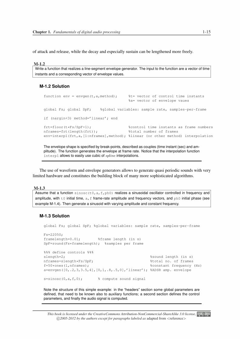
M-1.2Write a function that realizes a line-segment envelope generator. The input to the function are a vector of timeinstants and a corresponding vector of envelope values.
M-1.2 Solution
function env = envgen(t,a,method); %t= vector of control time instants%a= vector of envelope vaues
global Fs; global SpF; %global variables: sample rate, samples-per-frame
if (nargin<3) method=’linear’; end
frt=floor(t*Fs/SpF+1); %control time instants as frame numbersnframes=frt(length(frt)); %total number of framesenv=interp1(frt,a,[1:nframes],method); %linear (or other method) interpolation
The envelope shape is specified by break-points, described as couples (time instant (sec) and am-plitude). The function generates the envelope at frame rate. Notice that the interpolation functioninterp1 allows to easily use cubic of spline interpolations.
The use of waveform and envelope generators allows to generate quasi periodic sounds with verylimited hardware and constitutes the building block of many more sophisticated algorithms.
M-1.3Assume that a function sinosc(t0,a,f,ph0) realizes a sinusoidal oscillator controlled in frequency andamplitude, with t0 initial time, a,f frame-rate amplitude and frequency vectors, and ph0 initial phase (seeexample M-1.4). Then generate a sinusoid with varying amplitude and constant frequency.
M-1.3 Solution
global Fs; global SpF; %global variables: sample rate, samples-per-frame
Fs=22050;framelength=0.01; %frame length (in s)SpF=round(Fs*framelength); %samples per frame
%%% define controls %%%slength=2; %sound length (in s)nframes=slength*Fs/SpF; %total no. of framesf=50*ones(1,nframes); %constant frequency (Hz)a=envgen([0,.2,3,3.5,4],[0,1,.8,.5,0],’linear’); %ADSR amp. envelope
s=sinosc(0,a,f,0); % compute sound signal
Note the structure of this simple example: in the “headers” section some global parameters aredefined, that need to be known also to auxiliary functions; a second section defines the controlparameters, and finally the audio signal is computed.
This book is licensed under the CreativeCommons Attribution-NonCommercial-ShareAlike 3.0 license,c©2005-2012 by the authors except for paragraphs labeled as adapted from <reference>

1-16 Algorithms for Sound and Music Computing [v.March 13, 2012]
1.3.1.4 Frequency controlled oscillators
While realizing an amplitude modulated oscillator is quite straightforward, realizing a frequency mod-ulated oscillator requires some more work. First of all we have to understand what is the instantaneousfrequency of such an oscillator and how it relates to the phase function φ. This can be better under-stood in the continuous time domain. When the oscillator frequency is constant the phase is a linearfunction of time, φ(t) = 2πf0t. In the more general case in which the frequency varies at frame rate,the following equation holds:
f0(t) =12π
dφ
dt(t), (1.46)
which simply says that the instantaneous angular frequency ω0(t) = 2πf0(t) is the instantaneousangular velocity of the time-varying phase φ(t). If f0(t) is varying slowly enough (i.e. it is varying atframe rate), we can say that in the k-th frame the following first-order approximation holds:
12π
dφ
dt(t) = f0(t) ∼ f0(tk) + Fc [f0(tk+1)− f0(tk)] · (t− tk), (1.47)
where tk, tk+1 are the initial instants of frames k and k+1, respectively. The term Fc [f0(tk+1)− f0(tk)]approximates the derivative df0/dt inside the kth frame. We can then find the phase function by inte-grating equation (1.47):
φ(t) = φ(tk) + 2πf0(tk)(t− tk) + 2πFc[f0(tk+1)− f0(tk)](t− tk)2
2. (1.48)
From this equation, the discrete-time signal φ[n] can be computed within the kth frame, i.e. for thetime indexes (k − 1) · SpF + n, with n = 0 . . . (SpF− 1).
In summary, Eq. (1.48) allows to compute φ[n] at sample rate inside the kth frame, given theframe rate frequency values f0(tk) and f0(tk+1). The key ingredient of this derivation is the linearinterpolation (1.47).
M-1.4Realize the sinosc(t0,a,f,ph0) function that we have used in M-1.3. Use equation (1.48) to compute
the phase given the frame-rate frequency vector f.
M-1.4 Solution
function s = sinosc(t0,a,f,ph0);
global Fs; global SpF; %global variables: sample rate, samples-per-frame
nframes=length(a); %total number of framesif (length(f)==1) f=f*ones(1,nframes); endif (length(f)˜=nframes) error(’wrong f length!’); end
s=zeros(1,nframes*SpF); %initialize signal vector to 0lasta=a(1); lastf=f(1); lastph=ph0; %initialize amplitude, frequency, phase
for i=1:nframes %cycle on the framesnaux=1:SpF; %count samples within frame%%%%%%%%%%%% compute amplitudes and phases within frame %%%%%%%%%%%%%ampl=lasta + (a(i)-lasta)/SpF.*naux;phase=lastph +pi/Fs.*naux.*(2*lastf +(1/SpF)*(f(i)-lastf).*naux);%%%%%%%%%%%%%%%% read from table %%%%%%%%%%%%%%%%%%%%%%%%%%%%%%%%%%%
This book is licensed under the CreativeCommons Attribution-NonCommercial-ShareAlike 3.0 license,c©2005-2012 by the authors except for paragraphs labeled as adapted from <reference>

Chapter 1. Fundamentals of digital audio processing 1-17
0 0.5 1 1.5 2 2.5 3 3.5 40
0.2
0.4
0.6
0.8
1
t (s)
ampl
itude
(ad
im)
(a)
0 0.5 1 1.5 2 2.5 3 3.5 4180
200
220
240
260
t (s)
freq
uenc
y (H
z)
(b)
Figure 1.6: Amplitude (a) and frequency (b) control signals
s(((i-1)*SpF+1):i*SpF)=ampl.*cos(phase); %read from table%%%%%%%%% save last values of amplitude, frequency, phaselasta=a(i); lastf=f(i); lastph=phase(SpF);
ends=[zeros(1,round(t0*Fs)) s]; %add initial silence of t0 sec.
Both the amplitude a and frequency f envelopes are defined at frame rate and are interpolated atsample rate inside the function body. Note in particular the computation of the phase vector withineach frame.
We can finally listen to a sinudoidal oscillator controlled both in amplitude and in frequency.
M-1.5Synthesize a sinusoid modulated both in amplitude and frequency, using the functions sinosc and envgen.
M-1.5 Solution
global Fs; global SpF; %global variables: sample rate, samples-per-frame
Fs=22050;framelength=0.01; %frame length (in s)SpF=round(Fs*framelength); %samples per frame
%%% define controls %%%a=envgen([0,.2,3,3.5,4],[0,1,.8,.5,0],’linear’); %ADSR amp. envelopef=envgen([0,.2,3,4],[200,250,250,200],’linear’); %pitch envelopef=f+max(f)*0.05*... %pitch envelope with vibrato added
sin(2*pi*5*(SpF/Fs)*[0:length(f)-1]).*hanning(length(f))’;
%%% compute sound %%%s=sinosc(0,a,f,0);
Amplitude a and frequency f control signals are shown in Fig. 1.6.
This book is licensed under the CreativeCommons Attribution-NonCommercial-ShareAlike 3.0 license,c©2005-2012 by the authors except for paragraphs labeled as adapted from <reference>
1-18 Algorithms for Sound and Music Computing [v.March 13, 2012]
1.3.2 Noise generators
Up to now, we have considered signals whose behavior at any instant is supposed to be perfectlyknowable. These signals are called deterministic signals. Besides these signals, random signals ofunknown or only partly known behavior may be considered. For random signals, only some generalcharacteristics, called statistical properties, are known or are of interest. The statistical propertiesare characteristic of an entire signal class rather than of a single signal. A set of random signalsis represented by a random process. Particular numerical procedures simulate random processes,producing sequences of random (or more precisely, pseudorandom) numbers.
Random sequences can be used both as signals (i.e., to produce white or colored noise used as in-put to a filter) and a control functions to provide a variety in the synthesis parameters most perceptibleby the listener. In the analysis of natural sounds, some characteristics vary in an unpredictable way;their mean statistical properties are perceptibly more significant than their exact behavior. Hence, theaddition of a random component to the deterministic functions controlling the synthesis parametersis often desirable. In general, a combination of random processes is used because the temporal orga-nization of the musical parameters often has a hierarchical aspect. It cannot be well described by asingle random process, but rather by a combination of random processes evolving at different rates.For example this technique is employed to generate 1/f noise.
1.3.2.1 White noise generators
The spread part of the spectrum is perceived as random noise. In order to generate a random sequence,we need a random number generator. There are many algorithms that generate random numbers,typically uniformly distributed over the standardized interval [0, 1). However it is hard to find goodrandom number generators, i.e. that pass all or most criteria of randomness. The most commonis the so called linear congruential generator. It can produce fairly long sequences of independentrandom numbers, typically of the order of two billion numbers before repeating periodically. Givenan initial number (seed) I[0] inn the interval 0 ≤ I[0] < M , the algorithm is described by the recursiveequations
I[n] = ( aI[n− 1] + c ) mod M (1.49)
u[n] = I[n]/M
where a and c are two constants that should be chosen very carefully in order to have a maximallength sequence, i.e. long M samples before repetition. The actual generated sequence depends onthe initial value I[0]; that is way the sequence is called pseudorandom. The numbers are uniformlydistributed over the interval 0 ≤ u[n] < 1. The mean is E[u] = 1/2 and the variance is σ2
u = 1/12.The transformation s[n] = 2u[n] − 1 generates a zero-mean uniformly distributed random sequenceover the interval [−1, 1). This sequence corresponds to a white noise signal because the generatednumbers are mutually independent. The power spectral density is given by S(f) = σ2
u. Thus thesequence contains all the frequencies in equal proportion and exhibits equally slow and rapid variationin time.
With a suitable choice of the coefficients a and b, it produces pseudorandom sequences with flatspectral density magnitude (white noise). Different spectral shapes ca be obtained using white noiseas input to a filter.
M-1.6
This book is licensed under the CreativeCommons Attribution-NonCommercial-ShareAlike 3.0 license,c©2005-2012 by the authors except for paragraphs labeled as adapted from <reference>

Chapter 1. Fundamentals of digital audio processing 1-19
A method of generating a Gaussian distributed random sequence is based on the central limit theorem, whichstates that the sum of a large number of independent random variables is Gaussian. As exercise, implementa very good approximation of a Gaussian noise, by summing 12 independent uniform noise generators.
If we desire that the numbers vary at a slower rate, we can generate a new random number everyd sampling instants and hold the previous value in the interval (holder) or interpolate between twosuccessive random numbers (interpolator). In this case the power spectrum is given by
S(f) = |H(f)|2 σ2u
d
with
|H(f)| =∣∣∣∣sin(πfd/Fs)sin(πf/Fs)
∣∣∣∣for the holder and
|H(f)| = 1d
[sin(πfd/Fs)sin(πf/Fs)
]2
for linear interpolation.
1.3.2.2 Pink noise generators
1/f noise generators A so-called pink noise is characterized by a power spectrum that fall in fre-quency like 1/f :
S(f) =A
f. (1.50)
For this reason pink noise is also called 1/f noise. To avoid the infinity at f = 0, this behaviour isassumed valid for f ≥ fmin, where fmin is a desired minimum frequency. The spectrum is charac-terized by a 3 db per octave drop, i.e. S(2f) = S(f)/2. The amount of power contained within afrequency interval [f1, f2] is ∫ f2
f1
S(f)df = A ln(
f1
f2
)
This implies that the amount of power in any octave is the same. 1/f noise is ubiquitous in natureand is related to fractal phenomena. In audio domain it is known as pink noise. It represents thepsychoacoustic equivalent of the white noise because he approximately excites uniformly the criticalbands. The physical interpretation is a phenomenon that depends on many processes that evolve ondifferent time scales. So a 1/f signal can be generated by the sum of several white noise generatorsthat are filtered through first¡order filters having the time constants that are successively larger andlarger, forming a geometric progression.
M-1.7In the Voss 1/f noise generation algorithm, the role of the low pass filters is played by the hold filter seen in theprevious paragraph. The 1/f noise is generated by taking the average of several periodically held generatorsyi[n], with periods forming a geometric progression di = 2i, i.e.
y[n] =1
M
MXi=1
yi[n] (1.51)
The power spectrum does not have an exact 1/f shape, but it is close to it for frequencies f ≥ Fs/2M . Asexercise, implement a 1/f noise generator and use it to assign the pitches to a melody.
This book is licensed under the CreativeCommons Attribution-NonCommercial-ShareAlike 3.0 license,c©2005-2012 by the authors except for paragraphs labeled as adapted from <reference>

1-20 Algorithms for Sound and Music Computing [v.March 13, 2012]
M-1.8The music derived from the 1/f noise is closed to the human music: it does not have the unpredictability andrandomness of white noise nor the predictability of brown noise. 1/f processes correlate logarithmically withthe past. Thus the averaged activity of the last ten events has as much influence on the current value as thelast hundred events, and the last thousand. Thus they have a relatively long-term memory.1/f noise is a fractal one; it exhibits self-similarity, one property of the fractal objects. In a self-similar se-quence, the pattern of the small details matches the pattern of the larger forms, but on a different scale. Inthis case, is used to say that 1/f fractional noise exhibits statistical self-similarity. The pink noise algorithm forgenerating pitches has become a standard in algorithmic music. Use the 1/f generator developed in M-1.7 toproduce a fractal melody.
1.4 Spectral analysis of discrete-time signals
Spectral analysis is one of the powerful analysis tool in several fields of engineering. The fact that wecan decompose complex signals with the superposition of other simplex signals, commonly sinusoidor complex exponentials, highlights some signal features that sometimes are very hard to discoverotherwise. Furthermore, the decomposition on simpler functions in the frequency domain is veryuseful when we want to perform modifications on a signal, since it gives the possibility to manipulatesingle spectral components, which is hard if not impossible to do on the time-domain waveform.
A rigorous and comprehensive tractation of spectral analysis is out the scope of this book. In thissection we introduce the Discrete-Time Fourier Transform (DTFT), which the discrete-time versionof the classical Fourier Transform of continuous-time signals. Using the DTFT machinery, we thendiscuss briefly the main problems related to the process of sampling a continuous-time signal, namelyfrequency aliasing. This discussion leads us to the sampling theorem.
1.4.1 The discrete-time Fourier transform
1.4.1.1 Definition
Recall that for a continuous-time signal x(t) the Fourier Transform is defined as:
Fx(ω) = X(ω) =∫ +∞
−∞x(t)e−j2πftdt =
∫ +∞
−∞x(t)e−jωtdt (1.52)
where the variable f is frequency and is expressed in Hz, while the angular frequency ω has beendefined as ω = 2πf and expressed in radians/s. Note that we are following the conventional notationby which time-domain signals are denoted using lowercase symbols (e.g., x(n)) while frequency-domain signals are denoted in uppercase (e.g., X(ω)).
We can try to find an equivalent expression in the case of a discrete-time signal x[n]. If we think ofx[n] as the sampled version of a continuous-time signal x(t) with a sampling interval Ts = 1/Fs, i.e.x[n] = x(nTs), we can define the discrete-time Fourier transform (DTFT) starting from Eq. (1.52)where the integral is substituted by a summation:
Fx(ωd) = X(ωd) =+∞∑
n=−∞x(nTs)e
−j2πf nFs =
+∞∑n=−∞
x[n]e−jωdn. (1.53)
There are two remarks to be made about this equation. First, we have omitted the scaling factor Ts
in front of the summation, which would be needed to have a perfect correspondence with Eq. (1.52)
This book is licensed under the CreativeCommons Attribution-NonCommercial-ShareAlike 3.0 license,c©2005-2012 by the authors except for paragraphs labeled as adapted from <reference>

Chapter 1. Fundamentals of digital audio processing 1-21
but is irrelevant to our tractation. Second, we have defined a new variable ωd = 2πf/Fs: we call thisthe normalized (or digital) angular frequency. This is not to be confused with the angular frequencyω used in Eq. (1.52): ωd is measured in radians/sample, and varies in the range [−2π, 2π] when fvaries in the range [−Fs, Fs]. In this book we use the notation ω to indicate the angular frequency inradians/s, and ωd to indicate the normalized angular frequency in radians/sample.
As one can verify from Eq. (1.53), X(ωd) is a periodic function in ωd with a period 2π. Note thatthis periodicity of 2π in ωd corresponds to a periodicity of Fs in the domain of the absolute-frequencyf . Moreover X(ωd) is in general a complex function, and can thus be written in terms of its real andimaginary parts, or alternatively in polar form as
X(ωd) = |X(ωd) | earg[X(ωd)], (1.54)
where |X(ωd) | is the magnitude function and arg[X(ωd)] is the phase function. Both are real-valuedfunctions. Given the 2π periodicity of X(ωd) we will arbitrarily assume that −π < arg[X(ωd)] < π.We informally refer to |X(ωd) | also as the spectrum of x[n].
The inverse discrete-time Fourier transform (IDTFT) is found by observing that Eq. (1.53) rep-resents the Fourier series of the periodic function X(ωd). As a consequence, one can apply Fouriertheory for periodic functions of continuous variables, and compute the Fourier coefficients x[n] as
F−1X[n] = x[n] =12π
∫ π
−πX(ωd)ejωdndωd. (1.55)
Equations (1.53) and (1.55) together form a Fourier representation for the sequence x[n]. Equa-tion (1.55) can be regarded as a synthesis formula, since it represents x[n] as a superposition of in-finitesimally small complex sinusoids, with X(ωd) determining the relative amount of each sinusoidalcomponent. Equation (1.53) can be regarded as an analysis formula, since it provides an expressionfor computing X(ωd) from the sequence x[n] and determining its sinusoidal components.
1.4.1.2 DTFT of common sequences
We can apply the DTFT definition to some of the sequences that we have examined. The DTFT of theunit impulse δ[n] is the constant 1:
Fδ(ωd) =+∞∑
n=−∞δ[n]e−jωdn = 1. (1.56)
The unit step sequence u[n] does not have a DTFT, because the sum in Eq. (1.53) takes infinite values.The exponential sequence (1.9) also does not admit a DTFT. However if we consider the right sidedexponential sequence x[n] = anu[n], in which the unit step is multiplied by an exponential with| a | < 1, then this admits a DTFT:
Fx(ωd) =+∞∑
n=−∞anu[n]e−jωdn =
+∞∑
n=0
(ae−jωd
)n =1
1− ae−jωd. (1.57)
The complex exponential sequence x[n] = ejω0n or the real sinusoidal sequence x[n] = cos(ω0n+φ) are other examples of sequences that do not have a DTFT, because the sum in Eq. (1.53) takes in-finite values. In general a sequences does not necessarily admit a Fourier representation, meaningwith this that the series in Eq. (1.53) may not converge. One can show that x[n] being absolutely
This book is licensed under the CreativeCommons Attribution-NonCommercial-ShareAlike 3.0 license,c©2005-2012 by the authors except for paragraphs labeled as adapted from <reference>

1-22 Algorithms for Sound and Music Computing [v.March 13, 2012]
Property Time-domain sequences Frequency-domain DTFTsx[n], y[n] X(ωd), Y (ωd)
Linearity ax[n] + by[n] aX(ωd) + bY (ωd)Time-shifting x[n− n0] e−jωdn0X(ωd)
Frequency-shifting ejω0nx[n] X(ωd − ω0)
Frequency differentation nx[n] j dXdωd
(ωd)
Convolution (x ∗ y)[n] X(ωd) · Y (ωd)Multiplication x[n] · y[n] 1
2π
∫ π−π X(θ)Y (ωd − θ)dθ
Parseval relation+∞∑
n=−∞x[n]y∗[n] =
12π
∫ π
−πX(ωd)Y ∗(ωd)dωd
Table 1.1: General properties of the discrete-time Fourier transform.
summable (we have defined absolute summability in Eq. (1.32)) is a sufficient condition for the con-vergence of the series (recall the definition of absolute summability given in Eq. (1.32)). Note that anabsolutely summable sequence has always finite energy, and that the opposite is not always true, since∑ |x[n] |2 ≤ (
∑ |x[n] |)2. Therefore a finite-energy sequence does not necessarily admit a Fourierrepresentation.2
1.4.1.3 Properties
Table 1.1 lists a number of properties of the DTFT which are useful in digital signal processingapplications. Time- and frequency-shifting are interesting properties in that they show that a shiftingoperation in either domain correspond to multiplication for an complex exponential function in theother domain. Proof of these properties is straightforward from the definition of DTFT.
The convolution property is extremely important: it says that a convolution in the time domainbecomes a simple multiplication in the frequency domain. This can be demonstrated as follows:
Fx ∗ y(ωd) =+∞∑
n=−∞
(+∞∑
k=−∞x[k]y[n− k]
)e−jωdn =
+∞∑m=−∞
+∞∑
k=−∞x[k]y[m]e−jωd(k+m)
=+∞∑
k=−∞x[k]e−jωdk ·
+∞∑m=−∞
y[m]e−jωdm,
(1.58)
where in the second equality we have substituted m = n − k. The multiplication property is dual tothe convolution property: a multiplication in the time-domain becomes a convolution in the frequencydomain.
The Parseval relation is also very useful: if we think of the sum on the left-hand side as an innerproduct between the sequences x and y, we can restate this property by saying that the DTFT preservesthe inner product (apart from the scaling factor 1/2π). In particular, when x = y, it preserves the
2For non-absolutely summable sequences like the unit step or the sinusoidal sequence, the DTFT can still be definedif we resort to the Dirac delta δD(ωd − ω0). Since this is not a function but rather a distribution, extending the DTFTformalism to non-summable sequences requires to dive into the theory of distributions, which we are not willing to do.
This book is licensed under the CreativeCommons Attribution-NonCommercial-ShareAlike 3.0 license,c©2005-2012 by the authors except for paragraphs labeled as adapted from <reference>

Chapter 1. Fundamentals of digital audio processing 1-23
0 0.2 0.4 0.6 0.8 1 1.2 1.4 1.6 1.8−1
−0.5
0
0.5
1
t (s)
ampl
itude
x1(t)
x2(t)
x3(t)
x1,2,3
[n]
Figure 1.7: Example of frequency aliasing occurring for three sinusoids.
energy of the signal x. The Parseval relation can be demonstrated by noting that the DTFT of thesequence y∗[−n] is Y ∗(ωd). Then we can write:
F−1XY ∗[n] =12π
∫ π
−πX(ωd)Y ∗(ωd)ejωdndωd =
+∞∑
k=−∞x[k]y∗[k − n], (1.59)
where in the first equality we have simply used the definition of the IDTFT, while in the secondequality we have exploited the convolution property. Evaluating this expression for n = 0 proves theParseval relation.
1.4.2 The sampling problem
1.4.2.1 Frequency aliasing
With the aid of the DTFT machinery, we can now go back to the concept of “sampling” and introducesome fundamental notions. Let us start with an example.
Consider three continuous-time sinusoids xi(t) (i = 1, 2, 3) defined as
x1(t) = cos(6πt), x2(t) = cos(14πt), x3(t) = cos(26πt). (1.60)
These sinusoids have frequencies 3, 7, and 13 Hz, respectively. Now we construct three sequencesxi[n] = xi(n/Fs) (i = 1, 2, 3), each obtained by sampling one of the above signals, with a samplingfrequency Fs = 10 Hz. We obtain the sequences
x1[n] = cos(0.6πn), x2[n] = cos(1.4πn), x3[n] = cos(2.6πn). (1.61)
Figure 1.7 shows the plots of both the continuous-time sinusoids and the sampled sequences: note thatall sequences have exactly the same sample values for all n, i.e. they actually are the same sequence.This phenomenon of a higher frequency sinusoid acquiring the identity of a lower frequency sinusoidafter being sampled is called frequency aliasing.
In fact we can understand the aliasing phenomenon in a more general way using the Fourier theory.Consider a continuous-time signal x(t) and its sampled version xd[n] = x(nTs). The we can provethat the Fourier Transform X(ω) of x(t) and the DTFT Xd(ωd) of xd[n] are related via the followingequation:
Xd(ωd) = Fs
+∞∑m=−∞
X(ωdFs + 2mπFs). (1.62)
This book is licensed under the CreativeCommons Attribution-NonCommercial-ShareAlike 3.0 license,c©2005-2012 by the authors except for paragraphs labeled as adapted from <reference>
1-24 Algorithms for Sound and Music Computing [v.March 13, 2012]
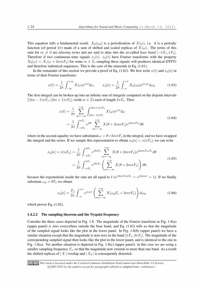
This equation tells a fundamental result: Xd(ωd) is a periodization of X(ω), i.e. it is a periodicfunction (of period 2π) made of a sum of shifted and scaled replicas of X(ω). The terms of thissum for m 6= 0 are aliasing terms and are said to alias into the so-called base band [−πFs, πFs].Therefore if two continuous-time signals x1(t), x2(t) have Fourier transforms with the propertyX2(ω) = X1(ω + 2mπFs) for some m ∈ Z, sampling these signals will produces identical DTFTsand therefore indentical sequences. This is the case of the sinusoids in Eq. (1.61).
In the remainder of this section we provide a proof of Eq. (1.62). We first write x(t) and xd[n] interms of their Fourier transforms:
x(t) =12π
∫ +∞
−∞X(ω)ejωtdω, xd[n] =
12π
∫ +π
−πXd(ωd)ejωdndωd. (1.63)
The first integral can be broken up into an infinite sum of integrals computed on the disjoint intervals[(2m− 1)πFs, (2m + 1)πFs], (with m ∈ Z) each of length 2πFs. Then
x(t) =12π
+∞∑m=−∞
∫ (2m+1)πFs
(2m−1)πFs
X(ω)ejωtdω
=12π
∫ πFs
−πFs
ejθt+∞∑
m=−∞X(θ + 2mπFs)ej2mπFstdθ,
(1.64)
where in the second equality we have substituted ω = θ+2mπFs in the integral, and we have swappedthe integral and the series. If we sample this representation to obtain xd[n] = x(nTs), we can write
xd[n] = x(nTs) =12π
∫ πFs
−πFs
ejθnTs
+∞∑m=−∞
X(θ + 2mπFs)ej2mπFsnTsdθ
=12π
∫ πFs
−πFs
ejθnTs
(+∞∑
m=−∞X(θ + 2mπFs)
)dθ,
(1.65)
because the exponentials inside the sum are all equal to 1 (ej2mπFsnTs = ej2nmπ = 1). If we finallysubstitute ωd = θTs we obtain
xd[n] =Fs
2π
∫ +π
−πejωdn
(+∞∑
m=−∞X(ωdFs + 2mπFs)
)dωd, (1.66)
which proves Eq. (1.62).
1.4.2.2 The sampling theorem and the Nyquist frequency
Consider the three cases depicted in Fig. 1.8. The magnitude of the Fourier transform in Fig. 1.8(a)(upper panel) is zero everywhere outside the base band, and Eq. (1.62) tells us that the magnitudeof the sampled signal looks like the plot in the lower panel. In Fig. 1.8(b) (upper panel) we have asimilar situation except that the magnitude is non-zero in the band [πFs, 3πFs]. The magnitude of thecorresponding sampled signal then looks like the plot in the lower panel, and is identical to the one inFig. 1.8(a). Yet another situation is depicted in Fig. 1.8(c) (upper panel): in this case we are using asmaller sampling frequency Fs, so that the magnitude now extends to more than one band. As a resultthe shifted replicas of |X | overlap and |Xd | is consequently distorted.
This book is licensed under the CreativeCommons Attribution-NonCommercial-ShareAlike 3.0 license,c©2005-2012 by the authors except for paragraphs labeled as adapted from <reference>

Chapter 1. Fundamentals of digital audio processing 1-25
Fs Fs
X( )ω
Fsdω
π π ω−
d ωX ( )d
... ...
(a)
Fs Fs
X( )ω
Fsdω
π π−
d ωX ( )d
ω
... ...
(b)
X( )ω
Fsdω
d ωX ( )d
Fsπ− Fsπ ω
... ...
(c)
Figure 1.8: Examples of sampling a continuous time signal: (a) spectrum limited to the base band;(b) the same spectrum shifted by 2π; (c) spectrum larger than the base band.
These examples suggest that a “correct” sampling of a continuos signal x(t) corresponds to thesituation of Fig. 1.8(a), while for the cases depicted in Figs. 1.8(b) and 1.8(c) we loose informationabout the original signal. The sampling theorem formalizes this intuition by saying that x(t) can beexactly reconstructed from its samples x[n] = x(nTs) if and only if X(ω) = 0 outside the base band(i.e. for all |ω | ≥ π/Fs). The frequency fNy = Fs/2 Hz, corresponding to the upper limit of the baseband, is called Nyquist frequency.
Based on what we have just said, when we sample a continuous-time signal we must choose Fs insuch a way that the Nyquist frequency is above any frequency of interest, otherwise frequencies abovefNy will be aliased. In the case of audio signals, we know from psychoacoustics that humans perceiveaudio frequencies up to ∼ 20 kHz: therefore in order to guarantee that no artifacts are introducedby the sampling procedure we must use Fs > 40 kHz, and in fact the most diffused standard isFs = 44.1 kHz. In some specific cases we may use lower sampling frequencies: as an example it isknown that the spectrum of a speech signal is limited to ∼ 4 kHz, and accordingly the most diffusedstandard in telephony is Fs = 8 kHz.
In the remainder of this section we sketch the proof of the sampling theorem. If X(ω)) 6= 0 onlyin the base band, then all the sum terms in Eq. (1.62) are 0 except for the one with m = 0. Therefore
Xd(ωd) = FsX(ωdFs) for ωd ∈ (−π, π). (1.67)
In order to reconstruct x(t) we can take the inverse Fourier Transform:
x(t) =12π
∫ +∞
−∞X(ω)ejωtdω =
12π
∫ πFs
−πFs
X(ω)ejωtdω =1
2πFs
∫ +πFs
πFs
Xd
(ω
Fs
)ejωtdω. (1.68)
where in the second equality we have exploited the hypothesis X ≡ 0 outside the base band and inthe third one we have used Eq. (1.67). If we now reapply the definition of the DTFT we obtain
x(t) =1
2πFs
∫ πFs
−πFs
[+∞∑
n=−∞x(nTs))e−jωTsn
]ejωtdω =
+∞∑n=−∞
x(nTs)2πFs
∫ πFs
−πFs
ejω(t−nTs)dω, (1.69)
where in the second equality we have swapped the sum with the integral. Now look at the integral on
This book is licensed under the CreativeCommons Attribution-NonCommercial-ShareAlike 3.0 license,c©2005-2012 by the authors except for paragraphs labeled as adapted from <reference>
1-26 Algorithms for Sound and Music Computing [v.March 13, 2012]
the right hand side. We can solve it explicitly and write
12πFs
∫ πFs
−πFs
ejω(t−nTs)dω =1
2πFs
22j(t− nTs)
[ejπFs(t−nTs) − e−jπFs(t−nTs)
]=
=sin[πFs(t− nTs)]
πFs(t− nTs)= sinc[Fs(t− nTs)].
(1.70)
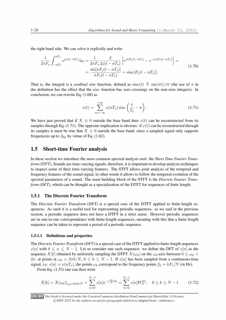
That is, the integral is a cardinal sine function, defined as sinc(t) , sin(πt)/πt (the use of π inthe definition has the effect that the sinc function has zero crossings on the non-zero integers). Inconclusion, we can rewrite Eq. (1.68) as
x(t) =+∞∑
n=−∞x(nTs) sinc
(t
Ts− n
). (1.71)
We have just proved that if X ≡ 0 outside the base band then x(t) can be reconstructed from itssamples through Eq. (1.71). The opposite implication is obvious: if x(t) can be reconstructed throughits samples it must be true that X ≡ 0 outside the base band, since a sampled signal only supportsfrequencies up to fNy by virtue of Eq. (1.62).
1.5 Short-time Fourier analysis
In these section we introduce the most common spectral analysis tool: the Short Time Fourier Trans-form (STFT). Sounds are time-varying signals, therefore, it is important to develop analysis techniquesto inspect some of their time-varying features. The STFT allows joint analysis of the temporal andfrequency features of the sound signal, in other words it allows to follow the temporal evolution of thespectral parameters of a sound. The main building block of the STFT is the Discrete Fourier Trans-form (DFT), which can be thought as a specialization of the DTFT for sequences of finite length.
1.5.1 The Discrete Fourier Transform
The Discrete Fourier Transform (DFT) is a special case of the DTFT applied to finite-length se-quences. As such it is a useful tool for representing periodic sequences. as we said in the previoussection, a periodic sequence does not have a DTFT in a strict sense. However periodic sequencesare in one-to-one correspondence with finite-length sequences, meaning with this that a finite-lengthsequence can be taken to represent a period of a periodic sequence.
1.5.1.1 Definitions and properties
The Discrete Fourier Transform (DFT) is a special case of the DTFT applied to finite-length sequencesx[n] with 0 ≤ n ≤ N − 1. Let us consider one such sequence: we define the DFT of x[n] as thesequence X[k] obtained by uniformly sampling the DTFT X(ωd) on the ωd-axis between 0 ≤ ωd <2π, at points at ωk = 2πk/N , 0 ≤ k ≤ N − 1. If x[n] has been sampled from a continuous-timesignal, i.e. x[n] = x(nTs), the points ωk correspond to the frequency points fk = kFs/N (in Hz).
From Eq. (1.53) one can then write
X[k] = X(ωd)|ωd=2πk/N =N−1∑
n=0
x[n]e−j 2πN
kn =N−1∑
n=0
x[n]W knN , 0 ≤ k ≤ N − 1 (1.72)
This book is licensed under the CreativeCommons Attribution-NonCommercial-ShareAlike 3.0 license,c©2005-2012 by the authors except for paragraphs labeled as adapted from <reference>

Chapter 1. Fundamentals of digital audio processing 1-27
where we have used the notation WN = e−j2π/N . Note that the DFT is also a finite-length sequencein the frequency domain, with length N . The inverse discrete Fourier Transform (IDFT) is given by
x[n] =1N
N−1∑
k=0
X[k]W−knN , 0 ≤ n ≤ N − 1. (1.73)
This relation can be verified by multiplying both sides by W lnN , with l integer, and summing the result
from n = 0 to n = N − 1:
N−1∑
n=0
x[n]W lnN =
1N
N−1∑
n=0
N−1∑
k=0
X[k]W−(k−l)nN =
1N
N−1∑
k=0
X[k]
[N−1∑
n=0
W−(k−l)nN
], (1.74)
where the last equality has been obtained by interchanging the order of summation. Now, the summa-tion
∑N−1n=0 W
−(k−l)nN has the interesting property that it takes the value N when k− l = rN (r ∈ Z),
and takes the value 0 for any other value of k and l. Therefore Eq. (1.74) reduces to the definition ofthe DFT, and therefore Eq. (1.73) is verified.
We have just proved that, for a length-N sequence x[n], the N values of its DTFT X(ωd) at pointsωd = ωk are sufficient to determine x[n], and hence X(ωd), uniquely. This justifies our definition ofDiscrete Fourier Transform of finite-length sequences given in Eq. (1.72). The DFT is at the heart ofdigital signal processing, because it is a computable transformation.
Most of the DTFT properties listed in Table 1.1 have a direct translation for the DFT. Clearly theDFT is linear. The time- and frequency-shifting properties still correspond to a multiplication by acomplex number, however these properties becomes periodic with period N . As an example, the timeshifting properties for the DFT becomes
xm[n] = x[n−m] ⇒ Xm[k] = W kmN X[k]. (1.75)
Clearly any shift of m+lN samples cannot be distinguished from a shift by m samples, since W kmN =
Wk(m+lN)N . In other words, the ambiguity of the shift in the time domain has a direct counterpart in
the frequency domain.The convolution property also holds for the DFT and is stated as follows:
z[n] = (x ∗ y)[n] ,N−1∑
m=0
x[n]y[n−m] ⇒ Z[k] = (X · Y )[k], (1.76)
where in this case the symbol ∗ indicates the periodic convolution. The proof of this property issimilar to the one given for the DTFT.
1.5.1.2 Resolution, leakage and zero-padding
Consider the complex exponential sequence x[n] = ejω0n over a finite number of points 0 ≤ n < N .In Sec. 1.2 we have already shown that this sequence is periodic over the interval [0, N ] only ifω0N = 2πk for some integer k. This implies that there are exactly N periodic complex exponentialsequences representable with N samples, i.e. those for which ω0 = 2πk0/N , with k0 = 0 . . . N − 1:these are the sequences x[n] = ej2πk0n/N = W−k0n
N . From the definitions of the DFT and the IDFTit follows immediately that X[k] = δ(k − k0), i.e. the DFT associated to the sequence W−k0n
N takesthe value 1 for k = k0 and is zero everywhere else. As an example, Fig. 1.9(a) shows a 64-points DFT(computed numerically) for the sequence x[n] = W−k0n
N for k0 = 20.
This book is licensed under the CreativeCommons Attribution-NonCommercial-ShareAlike 3.0 license,c©2005-2012 by the authors except for paragraphs labeled as adapted from <reference>
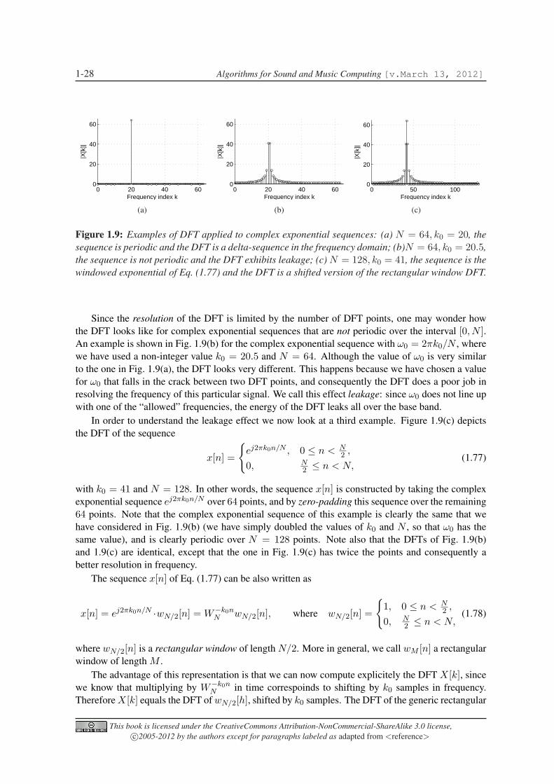
1-28 Algorithms for Sound and Music Computing [v.March 13, 2012]
0 20 40 600
20
40
60
Frequency index k
|X[k
]|
(a)
0 20 40 600
20
40
60
Frequency index k
|X[k
]|
(b)
0 50 1000
20
40
60
Frequency index k
|X[k
]|
(c)
Figure 1.9: Examples of DFT applied to complex exponential sequences: (a) N = 64, k0 = 20, thesequence is periodic and the DFT is a delta-sequence in the frequency domain; (b)N = 64, k0 = 20.5,the sequence is not periodic and the DFT exhibits leakage; (c) N = 128, k0 = 41, the sequence is thewindowed exponential of Eq. (1.77) and the DFT is a shifted version of the rectangular window DFT.
Since the resolution of the DFT is limited by the number of DFT points, one may wonder howthe DFT looks like for complex exponential sequences that are not periodic over the interval [0, N ].An example is shown in Fig. 1.9(b) for the complex exponential sequence with ω0 = 2πk0/N , wherewe have used a non-integer value k0 = 20.5 and N = 64. Although the value of ω0 is very similarto the one in Fig. 1.9(a), the DFT looks very different. This happens because we have chosen a valuefor ω0 that falls in the crack between two DFT points, and consequently the DFT does a poor job inresolving the frequency of this particular signal. We call this effect leakage: since ω0 does not line upwith one of the “allowed” frequencies, the energy of the DFT leaks all over the base band.
In order to understand the leakage effect we now look at a third example. Figure 1.9(c) depictsthe DFT of the sequence
x[n] =
ej2πk0n/N , 0 ≤ n < N
2 ,
0, N2 ≤ n < N,
(1.77)
with k0 = 41 and N = 128. In other words, the sequence x[n] is constructed by taking the complexexponential sequence ej2πk0n/N over 64 points, and by zero-padding this sequence over the remaining64 points. Note that the complex exponential sequence of this example is clearly the same that wehave considered in Fig. 1.9(b) (we have simply doubled the values of k0 and N , so that ω0 has thesame value), and is clearly periodic over N = 128 points. Note also that the DFTs of Fig. 1.9(b)and 1.9(c) are identical, except that the one in Fig. 1.9(c) has twice the points and consequently abetter resolution in frequency.
The sequence x[n] of Eq. (1.77) can be also written as
x[n] = ej2πk0n/N ·wN/2[n] = W−k0nN wN/2[n], where wN/2[n] =
1, 0 ≤ n < N
2 ,
0, N2 ≤ n < N,
(1.78)
where wN/2[n] is a rectangular window of length N/2. More in general, we call wM [n] a rectangularwindow of length M .
The advantage of this representation is that we can now compute explicitely the DFT X[k], sincewe know that multiplying by W−k0n
N in time correspoinds to shifting by k0 samples in frequency.Therefore X[k] equals the DFT of wN/2[h], shifted by k0 samples. The DFT of the generic rectangular
This book is licensed under the CreativeCommons Attribution-NonCommercial-ShareAlike 3.0 license,c©2005-2012 by the authors except for paragraphs labeled as adapted from <reference>

Chapter 1. Fundamentals of digital audio processing 1-29
0 50 1000
20
40
60
Frequency index k
Mag
nitu
de
(a)
0 50 1000
20
40
60
Frequency index k
Mag
nitu
de(b)
0 50 1000
20
40
60
Frequency index k
Mag
nitu
de
(c)
Figure 1.10: Examples of DFT (N = 128) applied to a rectangular window: (a) M = N/16, (b)M = N/8, (a) M = N/2.
window wM [n] can be computed from the definition as
FwM[k] =N−1∑
n=0
wM [n]W knN =
M−1∑
n=0
W knN =
1−W kMN
1−W kN
= e−j πkN
(M−1) sin(π kMN )
sin(π kN )
, (1.79)
where in the third equality we have used the property of the geometric series∑M−1
k=0 qk = (1 −qM )/(1 − q), and in the fourth equality we have applied some straigthforward trigonometry. Fig-ure 1.10 shows three plots of this DFT, for different window lengths M . In particular Fig. 1.10(c)shows the case M = N/2: note that this plot coincides with the one in Fig. 1.9(c), except for a shiftin frequency, which is what we expected.
To summarize, in this section we have shown that (a) the frequency resolution of the DFT islimited by the number N of DFT points, (b) the DFT of a complex exponential sequence which isnot periodic over N points exhibits poor resolution and leakage, and (c) the leakage effect can beinterpreted as the effect of a rectangular window of length N applied to the sequence.
M-1.9Compute the DFT of complex exponential sequence x[n] = ej2πk0n/N for integer and non-integer values of k0,in order to explore leakage effects. Then ompute the DFT of zero-padded complex exponential sequences, inorder to see how frequency resolution and leakage are affected.
1.5.1.3 Fast computation of the DFT: the FFT algorithm
A brute-force approach to DFT computation has O(N2
)running time, since we need to perform
O(N) multiplications and additions to compute each of the N DFT samples: we need more efficientsolutions to the problem. The Fast Fourier Transform (FFT) algorithm provides the most efficientcomputation of the DFT, as it runs in O(N log N) times. The algorithm is based on a divide-and-conquer strategy, that allows to compute the DFT of x[n] using the DFTs of two half-length subse-quences of x[n]. Additionally it exploits some nice properties of the N -th roots of unity W k
N .Assume for simplicity that the sequence x[n] has length N = 2s for some s ∈ N. Then we can
This book is licensed under the CreativeCommons Attribution-NonCommercial-ShareAlike 3.0 license,c©2005-2012 by the authors except for paragraphs labeled as adapted from <reference>

1-30 Algorithms for Sound and Music Computing [v.March 13, 2012]
write the DFT sequence X[k] as
X[k] =
N2−1∑
n=0
x[2n]W 2knN +
N2−1∑
n=0
x[2n + 1]W k(2n+1)N
=
N2−1∑
n=0
x[2n]W 2knN + W k
N
N2−1∑
n=0
x[2n + 1]W 2knN
=
N2−1∑
n=0
x[2n]W knN/2 + W k
N
N2−1∑
n=0
x[2n + 1]W knN/2,
(1.80)
where in the first equality we have separated the terms involving even elements and odd elements, inthe second one we have factorized a term W k
N , and in the third one we have exploited the propertyW ak
aN = W kN for any a ∈ N. If we now look at the two sums in the last row, we see that they are
the DFTs of the sequences x0[n] = x[0], x[2], . . . x[N − 2] and x1[n] = x[1], x[3], . . . x[N − 1],respectively. Both x0[n] and x1[n] have length N/2. Therefore the problem of computing X[k]reduces to the problem of computing two half-length DFTs X0[k], Xi[k], and then summing theirvalues according to Eq. (1.80). The resulting computational procedure is detailed in Algorithm 1.1.It is quite obvious that the running time T (N) of this algorithm is given by the recurrence equationT (N) = 2T (N/2) +O(N), therefore T (N) = O(N log N).
Algorithm 1.1: RECURSIVE-FFT(x)
N ← length(x) ;1
if n = 1 then return x ;2
WN = e−2πj/N ; W = 1 ;3
x0[n] = x[0], x[2], . . . x[N − 2]; x1[n] = x[1], x[3], . . . x[N − 1] ;4
X0[k] =RECURSIVE-FFT(x0) ;5
X1[k] =RECURSIVE-FFT(x1) ;6
for k ← 0 to N/2− 1 do7
X[k]← X0[k] + WX1[k] ;8
X[k + N/2]← X0[k]−WX1[k] ;9
W ←W ·WN ;10
return X11
M-1.10Realize Algorithm 1.1 and assess its functioning by comparing it with the fft function.
1.5.1.4 Iterative FFT algorithms and parallel realizations
Note that in writing the last cycle of Algorithm 1.1 we have exploited a relevant property of the W kN
coefficients, namely W(k+N/2)N = −W k
N . Thanks to this property the value WX1[k] is used twice(it is a common subexpression): first it is added to X0[k] to compute X[k], then it is subtracted fromX0[k] to compute X[k + N/2]. This is known as butterfly operation, and is the key element in theconstruction of a more efficient, iterative implementation of the FFT algorithm.
This book is licensed under the CreativeCommons Attribution-NonCommercial-ShareAlike 3.0 license,c©2005-2012 by the authors except for paragraphs labeled as adapted from <reference>

Chapter 1. Fundamentals of digital audio processing 1-31
Figure 1.11(a) depicts the tree of calls in an invocation of the recursive algorithm, in the caseN = 8. Looking at the tree we observe that, if we could arrange the elements in the order in whichthey appear in the leaves, we could compute the DFT as follows: first we take the elements in pairsand combine each pair with one butterfly operation, thus obtaining four 2-element DFTs; second, wetake these DFTs in pairs and combine each pair with two butterfly operations, thus obtaining two 4-element DFTs; finally, we combine these two DFTs with four butterfly operations, thus obtaining thefinal 8-element DFT. The resulting scheme is an iterative FFT implementation.
The only problem left is how to arrange the elements in the order in which they appear in theleaves. Luckily the solution is straightforward: this order is a bit-reversal permutation, that is x[n] isplaced in the position obtained by reversing the bits of the binary representation of n. We can thenwrite Algorithm 1.2. Clearly the algorithm is still O(N log N), since the total number of butterflyoperations isO(N log N), and since the bit-reversal permutation is also aO(N log N) procedure (wehave to reverse N integers, each made of log N bits). Figure 1.11(b) shows an efficient parallel im-plementation of this algorithm: it is made of log N stages, each performing N/2 butterfly operations.
Algorithm 1.2: ITERATIVE-FFT(x)
BIT-REVERSE-COPY(x, X) ;1
N ← length(x) ;2
for s← 1 to log2(N) do3
m← 2s; Wm = e2πj/m;4
for k ← 0 to N − 1 by m do5
W = 1;6
for l← 0 to m/2− 1 do7
t←WX[k + l + m/2]; u← X[k + l];8
X[k + l]← u + t; X[k + l + m/2]← u− t;9
W ←W ·Wm ;10
return X11
M-1.11Realize Algorithm 1.2 and assess its functioning by comparing it with the fft function.
1.5.2 The Short-Time Fourier Transform
1.5.2.1 Definition and examples
Xn(ωd) =+∞∑
m=−∞w[n−m]x[m]e−jωdm (1.81)
If w ≡ 1, then this equation reduces to the DTFT of x[n]. However in practical applications weare interested in using finite-length windows, in order to analyze the spectral properties of x[n] overa finite time interval. In such applications what we really do is computing, for each n, the DFT ofthe finite-length sequence w[n − m]x[m], and what we obtain is a finite-length sequence Xn[k] =Xn(ωd)|ωd=2πk/N .
This book is licensed under the CreativeCommons Attribution-NonCommercial-ShareAlike 3.0 license,c©2005-2012 by the authors except for paragraphs labeled as adapted from <reference>
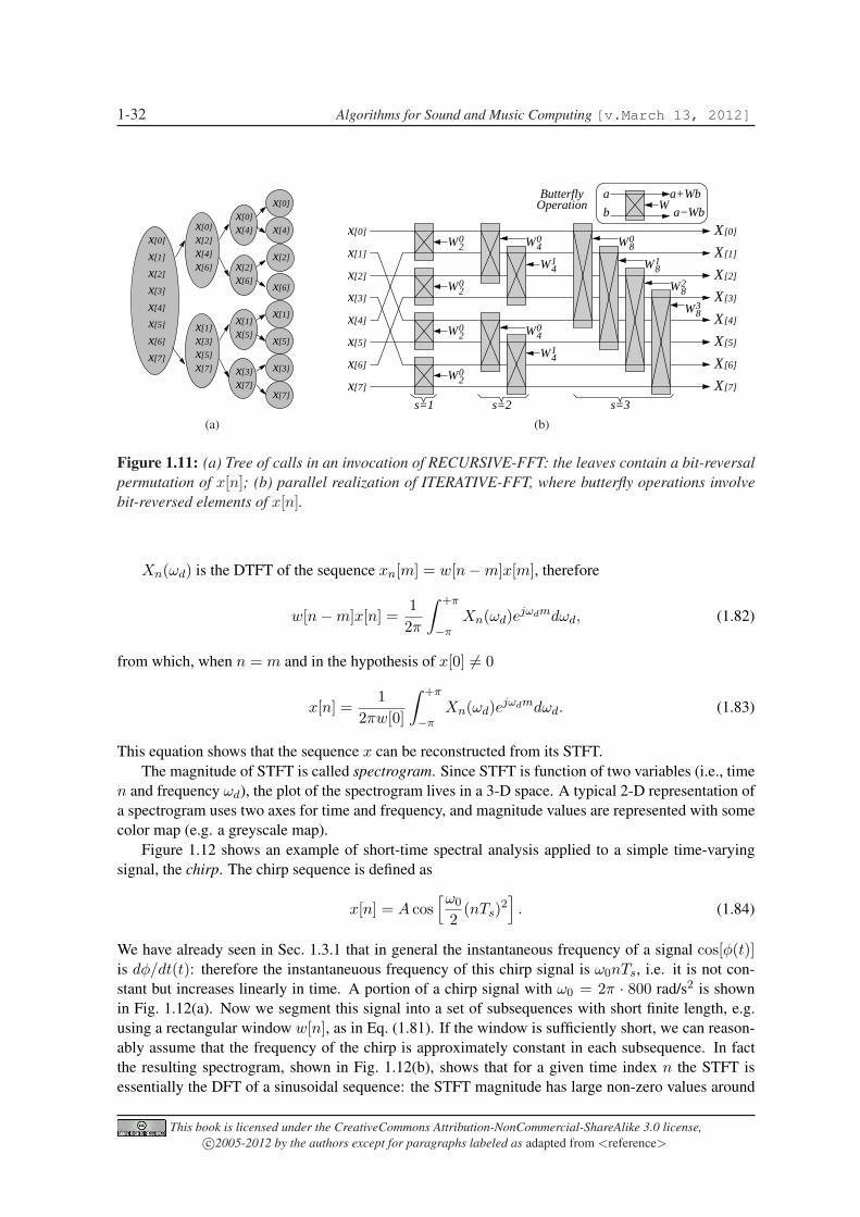
1-32 Algorithms for Sound and Music Computing [v.March 13, 2012]
x [0]
x [4]
x [2]
x [6]
x [1]
x [5]
x [3]
x [7]
x [3]
x [7]
x [0]
x [4]
x [6]
x [1]
x [5]
x [4]
x [3]
x [5]
x [7]
x [2]
x [0]
x [2]
x [6]
x [1]
x [7]
x [6]
x [5]
x [4]
x [3]
x [2]
x [1]
x [0]
(a)
x [0]
x [1]
x [2]
x [3]
x [4]
x [5]
x [7]
x [6]
2W0
2W0
2W0
2W0
[1]
[2]
[3]
[4]
[5]
[6]
[7]
[0]X
X
X
X
X
X
X
X
W41
W0
W
W
4
41
40
W
W1
W
W
8
8
8
8
0
2
3
OperationButterfly
Wb
a a+Wb
a−Wb
s=1 s=2 s=3
(b)
Figure 1.11: (a) Tree of calls in an invocation of RECURSIVE-FFT: the leaves contain a bit-reversalpermutation of x[n]; (b) parallel realization of ITERATIVE-FFT, where butterfly operations involvebit-reversed elements of x[n].
Xn(ωd) is the DTFT of the sequence xn[m] = w[n−m]x[m], therefore
w[n−m]x[n] =12π
∫ +π
−πXn(ωd)ejωdmdωd, (1.82)
from which, when n = m and in the hypothesis of x[0] 6= 0
x[n] =1
2πw[0]
∫ +π
−πXn(ωd)ejωdmdωd. (1.83)
This equation shows that the sequence x can be reconstructed from its STFT.The magnitude of STFT is called spectrogram. Since STFT is function of two variables (i.e., time
n and frequency ωd), the plot of the spectrogram lives in a 3-D space. A typical 2-D representation ofa spectrogram uses two axes for time and frequency, and magnitude values are represented with somecolor map (e.g. a greyscale map).
Figure 1.12 shows an example of short-time spectral analysis applied to a simple time-varyingsignal, the chirp. The chirp sequence is defined as
x[n] = A cos[ω0
2(nTs)2
]. (1.84)
We have already seen in Sec. 1.3.1 that in general the instantaneous frequency of a signal cos[φ(t)]is dφ/dt(t): therefore the instantaneuous frequency of this chirp signal is ω0nTs, i.e. it is not con-stant but increases linearly in time. A portion of a chirp signal with ω0 = 2π · 800 rad/s2 is shownin Fig. 1.12(a). Now we segment this signal into a set of subsequences with short finite length, e.g.using a rectangular window w[n], as in Eq. (1.81). If the window is sufficiently short, we can reason-ably assume that the frequency of the chirp is approximately constant in each subsequence. In factthe resulting spectrogram, shown in Fig. 1.12(b), shows that for a given time index n the STFT isessentially the DFT of a sinusoidal sequence: the STFT magnitude has large non-zero values around
This book is licensed under the CreativeCommons Attribution-NonCommercial-ShareAlike 3.0 license,c©2005-2012 by the authors except for paragraphs labeled as adapted from <reference>

Chapter 1. Fundamentals of digital audio processing 1-33
0 0.05 0.1 0.15 0.2−1
−0.5
0
0.5
1
t (s)
Am
plitu
de
(a)
t (s)f (
Hz)
0 1 2 3 40
1000
2000
3000
4000
(b)
t (s)
f (H
z)
0 1 2 3 40
500
1000
1500
2000
(c)
Figure 1.12: Short-time spectral analysis of a chirp signal: (a) initial portion of the chirp signal,with ω0 = 2π · 800 rad/s2; (b) spectrogram obtained with Fs = 8 kHz; (c) spectrogram obtained withFs = 4 kHz.
the instantaneous frequency, and much smaller non-zero values at other frequency points. More-over the instantaneous frequency increases linearly and after 5 seconds it reaches the value 4000 Hz(= 800 · 5 Hz), as expected.
So far in this example we have implicitely assumed that the sampling period Ts is sufficientlysmall, so that no aliasing occurs: in fact in drawing Fig. 1.12(b) we have used a sampling rate Fs =8 kHz. However, aliasing will occur if we use smaller sampling rates. Figure 1.12(c) shows thespectrogram obtained using Fs = 4 kHz: in this case frequencies above fNy = 2 kHz are aliased, andthis effect appears in the spectrogram when the black line starts moving down instead of increasing.
M-1.12Synthesize a chirp signal and compute its STFT using different sampling rates, in order to verify the occurrenceof aliasing.
1.5.2.2 Windowing and the uncertainty principle
We have previously examined the resolution and leakage problems associated to the DFT: decreasedfrequency resolution and spectral energy leakage occur because the spectrum is convolved with thatof a rectangular window. As the width of the rectangular window increases (see Fig. 1.10), the energyof its spectrum becomes more and more concentrated around the origin. In the limit, the spectrum ofan infinite-width rectangular window is a δ[k] sequence, and no leakage occurs.
This qualitative analysis provides an example of the so-called uncertainty principle. Increasingresolution in frequency diminishes resolution in time, and viceversa. Although a certain trade-offbetween time resolution and frequency resolution is inevitable (and determined by the window length),one may wonder if such a trade-off can be improved by using windows with different shapes (and thusdifferent spectra) from the rectangular window.
This book is licensed under the CreativeCommons Attribution-NonCommercial-ShareAlike 3.0 license,c©2005-2012 by the authors except for paragraphs labeled as adapted from <reference>

1-34 Algorithms for Sound and Music Computing [v.March 13, 2012]
−20 −10 0 10 200
0.2
0.4
0.6
0.8
1
Time index n
win
dow
(a)
0 50 100
−40
−30
−20
−10
0
Frequency index k
mag
nitu
de (
dB)
rectangularhannhammingblackman
(b)
Figure 1.13: Comparison of different windows; (a) time-domain window sequences, symmetrical withrespect to n = 0; (b) window spectra in the vicinity of k = 0. Differences in terms of main lobe widthand relative side lobe level can be appreciated.
In fact the answer is yes. Some of the most commonly used window functions are listed below:
(Hann) w[n] =12
[1 + cos
(2πn
2M + 1
)]
(Hamming) w[n] = 0.54 + 0.46 cos(
2πn
2M + 1
)
(Blackman) w[n] = 0.42 + 0.5 cos(
2πn
2M + 1
)+ 0.08 cos
(4πn
2M + 1
)(1.85)
Figure 1.13(a) depicts the plots of these windows in the time-domain, while a portion of the corre-sponding spectra is shown in Fig. 1.13(b). Note that these spectra share some common character-istics: all have large main “lobe” at 0 frequency, plus side lobes with decreasing amplitude. Moreprecisely, two main spectral features have to be taken into account when analyzing the properties ofthese windows: first, the ability to resolve two nearby spectral components of a windowed signal de-pend mostly on the main lobe width, i.e. the nearest zero crossings on both sides of the main lobe;second, the amount of leakage from one frequency component to neighbouring bands depends on theamplitude of the side lobes, and primarily on relative side lobe level, i.e. the difference in dB betweenthe amplitudes of the main lobe and the largest side lobe.
Figure 1.13(b) shows that the rectangular window has the smallest main lobe width, therefore it isbetter than other windows in resolving nearby sinusoids. On the other hand, it has the largest relativeside lobe level, therefore it causes considerable leakage. Other windows have different performancesin terms of main lobe width and relative side lobe level. The hamming window is often consideredto provide the best trade-off for short-term spectral analysis of generic signals, however the choice ofthe window to use depends in general on many factors, including the characteristics of the signal tobe analyzed.
M-1.13Compute the DFT of complex exponential sequences x[n] = ej2πk0n/N , windowed with rectangular, Hann,Hamming, and Blackman windows. Verify the performance of each window with respect to resolution andleakage effects, for integer and non-integer values of k0.
This book is licensed under the CreativeCommons Attribution-NonCommercial-ShareAlike 3.0 license,c©2005-2012 by the authors except for paragraphs labeled as adapted from <reference>

Chapter 1. Fundamentals of digital audio processing 1-35
Property Sequences z-Transforms ROCsx[n], y[n] X(z), Y (z) Rx, Ry
Linearity ax[n] + by[n] aX(z) + bY (z) contains Rx ∩Ry
Time-shifting x[n− n0] z−n0X(z) Rx
z-scaling zn0 x[n] X(z/z0) | z0 |Rx
z- differentation nx[n] −z dXdz (z) Rx
Conjugation x∗[n] X∗(z∗) Rx
Time-reversal x∗[−n] X∗(1/z∗) 1/Rx
Convolution (x ∗ y)[n] X(z) · Y (z) contains Rx ∩Ry
Initial value theorem If x[n] causal (i.e. x[n] = 0 ∀n < 0), then limz→∞X(z) = x[0].
Table 1.2: General properties of the z-Transform.
1.6 Digital filters
1.6.1 The z-Transform
1.6.1.1 Definitions
The z-Transform is an operator that maps a sequence of x[n] into a function X : C→ C. Definition:
Zx(z) = X(z) =+∞∑
n=−∞x[n]z−n, (1.86)
with z ∈ C complex variable.Close relationship with the DTFT: if z = ejωd , i.e. if we restrict the variable z to the complex
unit circle, then the z-Transform reduces to the DTFT. In particular the point z = 1 corresponds tofrequency ωd = 0, and z = −1 corresponds to ωd = π. Therefore evaluation of the z-Transformon the upper half of the complex unit circle gives the DTFT up to the (normalized angular) Nyquistfrequency. In general we can write:
Fx(ωd) = Zx(z)|z=ejωd . (1.87)
For this reason we sometimes write X(ejωd
)to indicate the DTFT of the sequence x.
The series in Eq. (1.86) does not converge for all values of z. For any sequence x, the set ofvalues z for which the series converges is called region of convergence (ROC). Since |X(z) | ≤∑+∞
n=−∞ |x[n] | | z |−n, if a point z0 belongs to the ROC, then all points z that are on the complexcircle with radius | z0 | also belong to the ROC. Therefore the ROC is in general a ring in the complexplane. Such ring may or may not include the unit circle, in other words the z-Transform of x[n] mayexist in a certain region of the complex plane even if the DTFT of x[n] does not exist.
Table 1.2 lists a set of relevant properties of the z-Transform, that are particularly useful in thestudy of discrete-time signals and digital filters. Most of them have direct counterparts in DTFTproperties (see Table 1.1), and can be proved from the definition (1.86).
The inverse z-transform is formally defined as
x[n] =1
2πj
∮
CX(z)zn−1dz, (1.88)
This book is licensed under the CreativeCommons Attribution-NonCommercial-ShareAlike 3.0 license,c©2005-2012 by the authors except for paragraphs labeled as adapted from <reference>

1-36 Algorithms for Sound and Music Computing [v.March 13, 2012]
where the integral is evaluated over the contour C, which can be any closed contour that belongs tothe ROC of X(z) and encircles z = 0. Without entering into details, we remark that for the kindsof sequences and z-transforms typically encountered in digital signal processing applications, lessformal procedures are sufficient and preferable. We propose some examples in Sec. 1.6.2.
1.6.1.2 z-transforms of common sequences
We illustrate the z-transform with some notable examples.The unit impulse δ[n] has z-transform 1 and the ROC is the entire complex plane. The ideal delay
δ[n− n0] has z-transform z−n0 and the ROC is the entire complex plane.Consider the finite-length exponential sequence
x[n] =
an, 0 ≤ n < N
0, elsewhere.(1.89)
The z-transform is
X(z) =N−1∑
n=0
anz−n =N−1∑
n=0
(az−1
)−n =1− aNz−N
1− az−1. (1.90)
In particular since the series has only a finite number of terms the ROC is the entire complex plane.We can generalize and state that any finite-length sequence admits a z-transform whose ROC is theentire complex plane.
Slightly more complex example: the right-sided exponential sequence x[n] = anu[n] alreadyexamined in Sec. 1.4.1. In this case
X(z) =+∞∑
n=−∞anu[n]z−n =
+∞∑
n=0
(az−1
)−n =1
1− az−1, (1.91)
where the last equality can be written only if∣∣ az−1
∣∣ < 1, otherwise the series does not converge.In other words the ROC is the region | z | > | a |. It is easy to verify that the left-sided exponentialsequence x[n] = −anu[−n] also has a z-transform, identical to the one in (1.91), but with a differentROC (the region | z | < | a |).
This example shows that the algebraic expression of the z-transform does not completely specifythe corresponding sequence, and that the ROC must also be specified. The example also shows a caseof a sequence that has a z-transform but does not have a DTFT: for a ≥ 1 the right-sided exponentialsequence still admits the z-transform 1/(1 − az−1) in the region | z | > a > 1 although it increasesexponentially in time and does not have a DTFT.
The right-sided real sinusoidal sequence x[n] = cos(ω0n)u[n]. Note that it can be written as asum of two exponential sequences: x[n] =
(ejω0nu[n] + e−jω0nu[n]
). Therefore
X(n) =12
[1
1− ejω0z−1+
11− e−jω0z−1
]= . . . =
1− [cosω0]z−1
1− 2[cosω0]z−1 + z−2. (1.92)
Since | cosω0 | ≤ 1, the ROC is clearly the region | z | > 1. This is a second example of a sequencethat does not admit a DTFT but admits a z-transform.
A final important example is the exponentially damped right-sided sinusoidal sequence, definedas x[n] = r−n cos(ω0n)u[n], with 0 < r < 1. In this case
X(n) =1− [r cosω0]z−1
1− 2[r cosω0]z−1 + r2z−2. (1.93)
This book is licensed under the CreativeCommons Attribution-NonCommercial-ShareAlike 3.0 license,c©2005-2012 by the authors except for paragraphs labeled as adapted from <reference>

Chapter 1. Fundamentals of digital audio processing 1-37
The ROC is the region | z | > r. Note that in this case the ROC includes the unit circle, thereforethe sequence x[n] also admits a DTFT. In fact as we will see this sequence represents the impulseresponse of a second-order resonating filter.
1.6.1.3 Rational z-transforms
A very important and useful family of z-transforms is that of rational transforms, i.e. those that canbe written as
X(z) =P (z)Q(z)
, with P (z), Q(z) polynomials. (1.94)
In fact in the previous section we have just examined a few examples of sequences with rationaltransforms, in particular the right-sided exponential sequence (1.91). Recalling that the z-transformis linear, we can say that any sequence that can be expressed as a linear combination of right-sidedexponentials has a rational z-transform.
x[n] =N∑
k=1
Akanku[n] ⇒ X(z) =
∑Nk=1 Ak
∏m6=k(1− amz−1)
∏Nk=1(1− akz−1)
(1.95)
The values z for which the P (z) = 0 (and therefore X(z) = 0) are called zeros of X(z). Thevalues z for which Q(z) = 0 are called poles of X(z). A number of important relations exist betweenthe poles of a rational transform and its ROC.
First, the ROC cannot contain poles by definition, since X(z) is not defined on the poles. It followsimmediately that a finite-length sequence cannot have any poles. As an example, looking at Eq. (1.90)one notices that the pole at z = a cancels with one of the zeros of the numerator (1 − aNz−N ),therefore there are no poles. In a similar line of reasoning one can prove that for any right-sidedsequence the ROC extends outwards from the pole with largest absolute value towards | z | → +∞,and that for any left-sided sequence the ROC extends inwards from the pole with smallest absolutevalue towards z → 0. For a generic sequence that extends infinitely on both sides, the ROC consistsof a ring bounded by a pole on the interior and exterior.
So-called pole-zero plots are typically used to represent z-transforms and their associated ROCs.Conventionally a zero is denoted with a “” symbol and a pole is denoted with a “×” symbol. As anexample. figure 1.14 shows the pole-zero plots for some of the transforms discussed in the previoussection. Note in particular that the right-sided and left-sided exponential sequences have identicalpole-zero patterns, but have different ROCs.
Since the pole-zero pattern does not completely define the corresponding sequence, it is sometimesconvenient to specify some time-domain properties of the sequences, that implicitly define the ROC.As an example, consider the pole-zero plot of either Fig. 1.14(b) or Fig. 1.14(c) and assume that theROC is not known. If one states that the corresponding sequence is absolutely summable, then thisimplies that it admits a DTFT and consequently implies that the ROC must be that of Fig. 1.14(c).Alternatively one may state that the corresponding sequence is causal: this implies that the ROC mustextend towards | z | → +∞ and consequently implies that the ROC must be that of Fig. 1.14(b).
1.6.2 Transfer function and frequency response of a LTI system
1.6.2.1 Definitions
In Sec. 1.2.3 we have seen that a LTI system is completely characterized by its impulse response h[n],since the response to any imput sequence x[n] can be written as the convolution between x and h (see
This book is licensed under the CreativeCommons Attribution-NonCommercial-ShareAlike 3.0 license,c©2005-2012 by the authors except for paragraphs labeled as adapted from <reference>

1-38 Algorithms for Sound and Music Computing [v.March 13, 2012]
aNN a
1
(a)
a
1
(b)
a
1
(c)
ω01
(d)
Figure 1.14: Pole-zero plots and ROCs of some simple transforms: (a) finite-length exponential se-quence; (b) right-sided exponential sequence with | a | > 1; (c) left-sided exponential sequence with| a | > 1; (d) exponentially damped, right-sided sinusoidal sequence. In all plots the dotted circle isthe unit circle and the gray-shaded region is the ROC of the corresponding transform.
Eqs. (1.22, 1.23)). Using the convolution property given in table 1.2, one can restate this by sayingthat for an LTI system an input sequence x is related to the corresponding output sequence y throughthe equation
Y (z) = H(z)X(z), (1.96)
where X(z), Y (z), H(z) are the z-transforms of x[n], y[n], h[n], respectively. We call H(z) thetransfer function of the LTI system. Assuming that an appropriate ROC is specified for H , we can saythat the LTI system is completely characterized by its transfer function.
If the ROC includes the unit circle, then h[n] admits a Fourier representation. In this case we canalso write
Y(ejωd
)= H
(ejωd
)X
(ejωd
), (1.97)
where X(ejωd
), Y
(ejωd
),H
(ejωd
)are the DTFTs of x[n], y[n], h[n], respectively. We call H
(ejωd
)the frequency response of the system. Assuming that the DTFTs are expressed in polar form (seeEq. (1.54)), we call
∣∣H(ejωd
) ∣∣ and arg[H
(ejωd
)]the magnitude response and the phase response
of the system, respectively.If the LTI system under consideration has been expressed through a constant-coefficient difference
equation (see Sec. 1.2.3), then one can immediately write the corresponding transfer function as arational function:
N∑
k=0
aky[n− k] =M∑
k=0
bkx[n− k] ⇔N∑
k=0
akz−kY (z) =
M∑
k=0
bkz−kX(z), (1.98)
from which it follows immediately that
H(z) =Y (z)X(z)
=∑M
k=0 bkz−k
∑Nk=0 akz−k
. (1.99)
Such z-transforms arise frequently in digital signal processing applications. By looking at a trans-form of this kind, one can easily find the corresponding sequence (this is an example of an informalprocedure for determining the z-transform). First one can note that H(z) can be written as
H(z) =b0
a0·∏M
k=1
(1− ckz
−1)
∏Nk=1 (1− dkz−1)
, (1.100)
This book is licensed under the CreativeCommons Attribution-NonCommercial-ShareAlike 3.0 license,c©2005-2012 by the authors except for paragraphs labeled as adapted from <reference>

Chapter 1. Fundamentals of digital audio processing 1-39
where the ck’s and the dk’s are the zeros and the poles of H , respectively. If M ≤ N and the polesare all first-order, then by applying a partial fraction expansion the above equation can be rewritten as
H(z) =N∑
k=1
Ak
1− dkz−1, with Ak =
(1− dkz
−1)H(z)|z=dk
. (1.101)
Looking back at Eq. (1.91), we can conclude that h[n] is a linear combination of right-sided exponen-tial sequences (or left-sided exponential sequences, depending on the ROC).
1.6.2.2 The concept of filtering
The magnitude and phase responses of a LTI system describe how the system transforms a sinusoidalinput x[n] = A cos(ω0n) = A
(ejω0 + e−jω0
)/2: the corresponding output is
y[n] = (h ∗ x)[n] = A∣∣ H
(ejω0
) ∣∣ · cos(ω0n + arg
[H
(ejω0
)]), (1.102)
i.e. the magnitude response at ω0 defines the gain and the phase delay of the system at the frequencyωd = ω0. Similar considerations apply to a generic input x[n]: the corresponding output can bedescribed in terms of system magnitude and phase response as
∣∣Y(ejωd
) ∣∣ =∣∣H
(ejωd
) ∣∣ · ∣∣X(ejωd
) ∣∣ ,
arg[Y
(ejωd
)]= arg
[H
(ejωd
)]+ arg
[X
(ejωd
)].
(1.103)
The first equation in (1.103) says that frequency components of the input are emphasized or attenuated(or even suppressed) depending on the values of
∣∣ H(ejωd
) ∣∣ at those frequencies. For this reasonwe typically refer to an LTI system as a frequency selective filter, or simply a filter. Thinking ofaudio, equalization is an obvious example of filtering an input sound by emphasizing certain frequencyranges and attenuating other ranges.
The second equation in (1.103) says that frequency components of the input are delayed in afrequency-dependent manner. The amount and type of tolerable phase distortion depends on theapplication. Often phase responses are disregarded in audio applications because phase distortionsare to a large extent inaudible. However taking into account the phase response can be important incertain cases, e.g. when one wants to preserve the shape of the time-domain waveform.
A generally tolerable type of phase distortion is linear distortion. A filter with a linear phaseresponse produces the same phase delay for all frequencies: as an example, the ideal delay systemhn0 = δ(n−n0) has a linear phase response arg
[Hn0
(ejωd
)]= ωdn0. A convenient measure of the
linearity of the phase response of a filter is the group delay, defined as3
τ(ωd) = − d
dωd
arg
[H
(ejωd
)]. (1.104)
The deviation of τ from a constant indicates the degree of phase non-linearity. Figure 1.15(a) providesa graphical comparison of the phase delay and the group delay.
The reason why τ is termed group delay is that this quantity relates to the effect of the phase on aquasi-sinusoidal signal. More precisely, consider the signal x[n] = a[n]eω0n, and assume that a[n] is
3Our definition uses ωd, so that τ is adimensional. Usual definitions employ ω, so that τ is in seconds.
This book is licensed under the CreativeCommons Attribution-NonCommercial-ShareAlike 3.0 license,c©2005-2012 by the authors except for paragraphs labeled as adapted from <reference>

1-40 Algorithms for Sound and Music Computing [v.March 13, 2012]
−φ0
(−slo
pe=g
roup
del
ay)
tang
ent t
o th
e cu
rve
line through the origin
(−slope=phase delay)
phaseresponse
ω
arg j ω
d
dH(e )
(a)
group
phasedelay
delay
x[n]
n
n
y[n]
(b)
Figure 1.15: Comparing phase delay and group delay: (a) evaluation of phase delay and groupdelay for a generic non-linear phase response; (b) illustration of phase delay and group delay for anarrowband signal.
varying slowly (equivalently, assume that the spectrum A(ejω) is concentrated near ω = 0). Then xwill look like the signal in Fig. 1.15(b) (upper panel). The signal can also be rewritten as
x[n] = a[n]eω0n =[
12π
∫ +ε
−εA(ejω)ejωndω
]eω0n, (1.105)
where ε ¿ π is the upper limit of the band of A. Therefore x can be viewed as a superposition ofneighboring sinusoidal components, or a group around ω0.
Since X(ejωd
) 6= 0 only in the vicinity of ω0), the phase response can be approximated in thatneighborhood as a line with slope −τ(ω0). With this approximation it is then quite straightforwardto show that the output is the filter output y[n] looks like in Fig. 1.15(b) (lower panel), i.e. τ(ω0)represents the delay applied to the slowly-varying amplitude a[n].
1.6.2.3 Stability, causality, and transfer functions
We have defined in Sec. 1.2.3 the notion of BIBO stability, and we have proved that an LTI system isstable if and only if its impulse response is absolutely summable. This latter condition can be rewrittenas
+∞∑n=−∞
∣∣h[n]z−n∣∣ <∞, (1.106)
for | z | = 1. Therefore the condition of stability is equivalent to the condition that the ROC of thetransfer function includes the unit circle. The examples depicted in Fig. 1.14 confirm this finding.
Consider the relevant particular case of rational transfer functions associated to causal systems:for these transfer functions the condition of stability is equivalent to the condition that all the polesare inside the unit circle, because the ROC extends outwards from the pole with the largest absolutevalue.
Another relevant particular case are FIR systems. We have alredy seen that a FIR system is alwaysstable since its impulse response is always absolutely summable. This property can be “seen” in thez domain by noting that the transfer function of a FIR system does not have poles, therefore the ROCis always the entire z plane and includes the unit circle.
This book is licensed under the CreativeCommons Attribution-NonCommercial-ShareAlike 3.0 license,c©2005-2012 by the authors except for paragraphs labeled as adapted from <reference>

Chapter 1. Fundamentals of digital audio processing 1-41
z−1
x[n]
y[n]
x[n]+y[n]
x[n]
a
ax[n]
x[n] x[n−1]
(a)
z−1
z−1
z−1
z−1
z−1
z−1
aN−1
bM
bM−1
b1
b0
a1
aN
y[n]x[n] 1
(b)
Figure 1.16: Block diagram representation of filters: (a) conventional pictorial symbols for delay,adder, and multiplier; (b) a general filter structure.
1.6.3 Digital filter structures and design approaches
In the following we only give a quick overview. In the next chapters we will discuss many specificfilters. In particular we will examine the second-order resonant filter in Chapter Sound modeling: signal
based approaches; comb and all-pass in Chapter Sound modeling: source based approaches; more comb and all-pass structures in Chapter Sound in space. We do not discusss filter structures (direct forms etc.), justa few words. Same with design techniques. In Chapter Sound modeling: source based approaches we talkabout bilinear transform, s-to-z mappings, impulse response invariance, all techniques used to designa digital filter from an analog one. In Chapter Sound in space we will see pole-zero approximations.
1.6.3.1 Block diagram representations
Most the LTI systems that we are going to realize are represented as linear constant coefficient equa-tions. As we have seen, the output of a LTI system represented in this way can be computed recursivelyprovided that past values of input and output are available. This values will undergo two operationsin the computation of the filter output: multiplication with coefficients, and addition.
Therefore the three basic elements for the implementation of a filter are memory for storing,past values, adders, and multipliers. A filter structure is created by properly interconnecting theseelements. Figure 1.16 shows the pictorial symbols that are typically used for representing them. Withthese elements, a general filter
y[n]−N∑
k=1
aky[n− k] =M∑
k=0
bkx[n− k] ⇒ H(z) =∑M
k=0 bkz−k
∑Nk=1 akz−k
(1.107)
can be represented with the block diagram of Fig. 1.16(b).
This book is licensed under the CreativeCommons Attribution-NonCommercial-ShareAlike 3.0 license,c©2005-2012 by the authors except for paragraphs labeled as adapted from <reference>

1-42 Algorithms for Sound and Music Computing [v.March 13, 2012]
ωdH( )
ωdH( )
ωc
ωc
ω
ω
d
d
low−pass
high−pass
(a)
ωdH( )
ωdH( )
ωc2ωc1
ωc1 ωc2
ω
ω
d
d
band−pass
band−reject
(b)
ωdH( )
ωdH( )
ωc
ωc
ω
ω
d
d
resonator
notch
(c)
Figure 1.17: Classification of filters into basic categories, depending on their magnitude response|H(ωd) |: (a) low-pass and high-pass filter; (b) band-pass and band-reject filter; (c) resonator andnotch filter.
1.6.3.2 Filter classification
Filters can be classified according to most salient characteristics of their frequency responses, mosttypically their magnitude. Basic filter categories are represented in Fig. 1.17. Other types of filterscan in general be described as a combination of these basic elements.
Low-pass filters (see Fig. 1.17(a), upper panel) select low frequencies up to a given cut-off fre-quency ωc, annd attenuate higher frequencies. High-pass filters (see Fig. 1.17(a), lower panel) havethe opposite behavior: they select frequencies above ωc, and attenuate lower frequencies.
Band-pass filters (see Fig. 1.17(b), upper panel) select frequencies within a frequency band, speci-fied by two cut-off frequencies ωc1 and ωc2, while frequencies outside this band are attenuated. Band-reject filters (see Fig. 1.17(b), lower panel) have the opposite behavior: they select frequencies outsidethe band [ωc1, ωc2], and attenuate frequencies within the band.
Resonator filters (see Fig. 1.17(c), upper panel) amplify frequencies in a narrow band around acut-off frequency ωc. Conversely, notch filters (see Fig. 1.17(c), lower panel) attenuate frequencies ina narrow band around ωc. Finally, when the magnitude response is perfectly flat the filter is called anall-pass filter, since all frequencies are passed. Note however that an all-pass filter modifies the phaseof the input signal. In the next chapter we will see some important uses of all-pass filters.
In order to optimize their frequency selective properties, ideal filters should have magnitude re-sponses exhibiting vertical transition between selected frequencies and rejected ones, Moreover theyshould have null or linear phase response in order not to introduce phase distortion. As an example,the ideal low-pass filter has the frequency response
Hlp
(ejω
)=
1, |ω | ≤ ωc,
0, ωc < |ω | ≤ π.(1.108)
However the corresponding impulse response is
hlp[n] =sinωcn
πn, −∞ < n < +∞, (1.109)
This book is licensed under the CreativeCommons Attribution-NonCommercial-ShareAlike 3.0 license,c©2005-2012 by the authors except for paragraphs labeled as adapted from <reference>

Chapter 1. Fundamentals of digital audio processing 1-43
i.e. the filter is non-causal and has a two-sided infinite impulse response. Therefore it is not possibleto compute its output either recursively or non-recursively. In other words, the filter is not realizable.Similar considerations apply to other types of ideal filters.
The simplest examples of realizable filters are first-order filters (i.e. filters with no more than onepole and/or one zero). First-order FIR low-pass and high-pass filters are defined as follows:
Hlp(z) =12
(1 + z−1
), Hhp(z) =
12
(1− z−1
). (1.110)
They have a zero in z = 1 and z = −1, respectively. Therefore the magnitude responses decrease andincrease monotically, respectively. The low-pass filter in particular can be recognized to be a movingaverage filter that averages two contiguous samples.
First-order IIR low-pass and high-pass filters are defined as follows:
Hlp(z) =1− α
21 + z−1
1− αz−1, Hhp(z) =
1 + α
21− z−1
1− αz−1. (1.111)
Both have a pole in z = α, therefore |α | < 1 for stability, and α ∈ R in order for the impulseresponses to be real-valued. They have a zero in z = 1 and z = −1, respectively. For α = 0 theyreduce to the FIR filters above, while for α > 0 they have steeper responses.
M-1.14Study the frequency responses of the first-order low-pass and high-pass filters of Eqs. (1.110, 1.111). Applythem to a broad-band audio signal (e.g. a snaredrum), and study their effect.
1.7 Commented bibliography
A general reference for digital signal processing is[Oppenheim et al., 1999]. Another classic is Mitra[2005]: more implementation oriented, with Matlab examples.
Primers on digital audio processing: Rocchesso [2003] and Steiglitz [1996]. Examples focusedon audio are found also in [Zolzer, 2002, Chapter 1]
A useful reading about Fourier analysis for discrete-time signals is provided in [Smith, 2008]. Ourdiscussion of FFT algorithms is based on [Cormen et al., 2001].
A discussion on recursive generators of sinusoidal signals is found e.g. in [Orfanidis, 1996].Models for fractal signals are also partially discussed in [Orfanidis, 1996].
ReferencesThomas H. Cormen, Charles E. Leiserson, Ronald L. Rivest, and Clifford Stein. Introduction to Algorithms. MIT Press,
Cambridge, MA, 2001.
Sanjit K Mitra. Digital Signal Processing. McGraw-Hill, third edition, 2005.
Alan V. Oppenheim, Ronald W. Schafer, and John R. Buck. Discrete-Time Signal Processing. Prentice Hall, Upper SaddleRiver, NJ, 1999.
Sophocles J. Orfanidis. Introduction to Signal Processing. Prentice Hall, 1996.
Davide Rocchesso. Introduction to Sound Processing. Mondo Estremo, Firenze, 2003. http://profs.sci.univr.it/˜rocchess/SP.
Julius O. Smith. Mathematics of the Discrete Fourier Transform (DFT). http://ccrma.stanford.edu/ jos/mdft/, 2008. Onlinebook, accessed Oct. 2008.
This book is licensed under the CreativeCommons Attribution-NonCommercial-ShareAlike 3.0 license,c©2005-2012 by the authors except for paragraphs labeled as adapted from <reference>

1-44 Algorithms for Sound and Music Computing [v.March 13, 2012]
Kenneth Steiglitz. A Digital Signal Processing Primer - With Applications to Digital Audio and Computer Music. PrenticeHall, 1996.
Udo Zolzer, editor. DAFX – Digital Audio Effects. John Wiley & Sons, 2002.
This book is licensed under the CreativeCommons Attribution-NonCommercial-ShareAlike 3.0 license,c©2005-2012 by the authors except for paragraphs labeled as adapted from <reference>

Contents
1 Fundamentals of digital audio processing 1-11.1 Introduction . . . . . . . . . . . . . . . . . . . . . . . . . . . . . . . . . . . . . . . 1-11.2 Discrete-time signals and systems . . . . . . . . . . . . . . . . . . . . . . . . . . . 1-1
1.2.1 Discrete-time signals . . . . . . . . . . . . . . . . . . . . . . . . . . . . . . 1-11.2.1.1 Main definitions . . . . . . . . . . . . . . . . . . . . . . . . . . . 1-11.2.1.2 Basic sequences and operations . . . . . . . . . . . . . . . . . . . 1-31.2.1.3 Measures of discrete-time signals . . . . . . . . . . . . . . . . . . 1-41.2.1.4 Random signals . . . . . . . . . . . . . . . . . . . . . . . . . . . 1-5
1.2.2 Discrete-time systems . . . . . . . . . . . . . . . . . . . . . . . . . . . . . 1-51.2.2.1 Basic systems and block schemes . . . . . . . . . . . . . . . . . . 1-61.2.2.2 Classes of discrete-time systems . . . . . . . . . . . . . . . . . . 1-6
1.2.3 Linear Time-Invariant Systems . . . . . . . . . . . . . . . . . . . . . . . . . 1-81.2.3.1 Impulse response and convolution . . . . . . . . . . . . . . . . . . 1-81.2.3.2 Properties of LTI systems . . . . . . . . . . . . . . . . . . . . . . 1-91.2.3.3 Constant-coefficient difference equations . . . . . . . . . . . . . . 1-10
1.3 Signal generators . . . . . . . . . . . . . . . . . . . . . . . . . . . . . . . . . . . . 1-121.3.1 Digital oscillators . . . . . . . . . . . . . . . . . . . . . . . . . . . . . . . . 1-12
1.3.1.1 Table lookup oscillator . . . . . . . . . . . . . . . . . . . . . . . 1-121.3.1.2 Recurrent sinusoidal signal generators . . . . . . . . . . . . . . . 1-131.3.1.3 Control signals and envelope generators . . . . . . . . . . . . . . 1-131.3.1.4 Frequency controlled oscillators . . . . . . . . . . . . . . . . . . . 1-16
1.3.2 Noise generators . . . . . . . . . . . . . . . . . . . . . . . . . . . . . . . . 1-181.3.2.1 White noise generators . . . . . . . . . . . . . . . . . . . . . . . 1-181.3.2.2 Pink noise generators . . . . . . . . . . . . . . . . . . . . . . . . 1-19
1.4 Spectral analysis of discrete-time signals . . . . . . . . . . . . . . . . . . . . . . . . 1-201.4.1 The discrete-time Fourier transform . . . . . . . . . . . . . . . . . . . . . . 1-20
1.4.1.1 Definition . . . . . . . . . . . . . . . . . . . . . . . . . . . . . . 1-201.4.1.2 DTFT of common sequences . . . . . . . . . . . . . . . . . . . . 1-211.4.1.3 Properties . . . . . . . . . . . . . . . . . . . . . . . . . . . . . . 1-22
1.4.2 The sampling problem . . . . . . . . . . . . . . . . . . . . . . . . . . . . . 1-231.4.2.1 Frequency aliasing . . . . . . . . . . . . . . . . . . . . . . . . . . 1-231.4.2.2 The sampling theorem and the Nyquist frequency . . . . . . . . . 1-24
1.5 Short-time Fourier analysis . . . . . . . . . . . . . . . . . . . . . . . . . . . . . . . 1-261.5.1 The Discrete Fourier Transform . . . . . . . . . . . . . . . . . . . . . . . . 1-26
1.5.1.1 Definitions and properties . . . . . . . . . . . . . . . . . . . . . . 1-261.5.1.2 Resolution, leakage and zero-padding . . . . . . . . . . . . . . . . 1-27
1-45

1-46 Algorithms for Sound and Music Computing [v.March 13, 2012]
1.5.1.3 Fast computation of the DFT: the FFT algorithm . . . . . . . . . . 1-291.5.1.4 Iterative FFT algorithms and parallel realizations . . . . . . . . . . 1-30
1.5.2 The Short-Time Fourier Transform . . . . . . . . . . . . . . . . . . . . . . . 1-311.5.2.1 Definition and examples . . . . . . . . . . . . . . . . . . . . . . . 1-311.5.2.2 Windowing and the uncertainty principle . . . . . . . . . . . . . . 1-33
1.6 Digital filters . . . . . . . . . . . . . . . . . . . . . . . . . . . . . . . . . . . . . . 1-351.6.1 The z-Transform . . . . . . . . . . . . . . . . . . . . . . . . . . . . . . . . 1-35
1.6.1.1 Definitions . . . . . . . . . . . . . . . . . . . . . . . . . . . . . . 1-351.6.1.2 z-transforms of common sequences . . . . . . . . . . . . . . . . . 1-361.6.1.3 Rational z-transforms . . . . . . . . . . . . . . . . . . . . . . . . 1-37
1.6.2 Transfer function and frequency response of a LTI system . . . . . . . . . . 1-371.6.2.1 Definitions . . . . . . . . . . . . . . . . . . . . . . . . . . . . . . 1-371.6.2.2 The concept of filtering . . . . . . . . . . . . . . . . . . . . . . . 1-391.6.2.3 Stability, causality, and transfer functions . . . . . . . . . . . . . . 1-40
1.6.3 Digital filter structures and design approaches . . . . . . . . . . . . . . . . . 1-411.6.3.1 Block diagram representations . . . . . . . . . . . . . . . . . . . 1-411.6.3.2 Filter classification . . . . . . . . . . . . . . . . . . . . . . . . . . 1-42
1.7 Commented bibliography . . . . . . . . . . . . . . . . . . . . . . . . . . . . . . . . 1-43
This book is licensed under the CreativeCommons Attribution-NonCommercial-ShareAlike 3.0 license,c©2005-2012 by the authors except for paragraphs labeled as adapted from <reference>