fundamentals of algorithms - free160592857366.free.fr/joe/ebooks/sharedata/eda... · in this...

CHAPTER

4Fundamentals ofalgorithms

Chung-Yang (Ric) HuangNational Taiwan University, Taipei, Taiwan

Chao-Yue LaiNational Taiwan University, Taipei, Taiwan

Kwang-Ting (Tim) ChengUniversity of California, Santa Barbara, California

ABOUT THIS CHAPTERIn this chapter, we will go through the fundamentals of algorithms that are

essential for the readers to appreciate the beauty of various EDA technologies

covered in the rest of the book. For example, many of the EDA problems can

be either represented in graph data structures or transformed into graph prob-lems. We will go through the most representative ones in which the efficient

algorithms have been well studied.

The readers should be able to use these graph algorithms in solving many of

their research problems. Nevertheless, there are still a lot of the EDA problems

that are naturally difficult to solve. That is to say, it is computationally infeasible

to seek for the optimal solutions for these kinds of problems. Therefore, heuris-

tic algorithms that yield suboptimal, yet reasonably good, results are usually

adopted as practical approaches. We will also cover several selected heuristicalgorithms in this chapter. At the end, we will talk about the mathematical pro-

gramming algorithms, which provide the theoretical analysis for the problem

optimality. We will especially focus on the mathematical programming problems

that are most common in the EDA applications.

4.1 INTRODUCTIONAn algorithm is a sequence of well-defined instructions for completing a task or

solving a problem. It can be described in a natural language, pseudocode, a flow-

chart, or even a programming language. For example, suppose we are interested

in knowing whether a specific number is contained in a given sequence of num-bers. By traversing the entire number sequence from a certain beginning number

173

to a certain ending number, we use a search algorithm to find this specific number.

Figure 4.1 illustrates this intuitive algorithm known as linear search.

Such kinds of algorithms can be implemented in a computer program andthen used in real-life applications [Knuth 1968; Horowitz 1978]. However, the

questions that must be asked before implementation are: “Is the algorithm effi-

cient?” “Can the algorithm complete the task within an acceptable amount of

time for a specific set of data derived from a practical application?” As we will

see in the next section, there are methods for quantifying the efficiency of an

algorithm. For a given problem, different algorithms can be applied, and each

of them has a different degree of efficiency. Such metrics for measuring an

algorithm’s efficiency can help answer the preceding questions and aid in theselection of the best possible algorithm for the task.

Devising an efficient algorithm for a given EDA problem could be challenging.

Because a rich collection of efficient algorithms already exists for a set of standard

problems where data are represented in the form of graphs, one possible

approach is to model the given problem as a graph problem and then apply a

known, efficient algorithm to solve the modeled graph problem. In Section 4.3,

we introduce several graph algorithms that are commonly used for a wide range

of EDA problems.Many EDA problems are intrinsically difficult, because finding an optimal

solution within a reasonable runtime is not always possible. For such problems,

certain heuristic algorithms can be applied to find an acceptable solution first.

If time or computer resources permit, such algorithms can further improve the

result incrementally.

In addition to modeling EDA problems in graphs, it is sometimes possible to

transform them into certain mathematical models, such as linear inequalities or

nonlinear equations. The primary advantage of modeling an EDA problem with

Inputs: a sequence of number S a number n

Let variable x = S.begin()

x == n ?

x == S.end() ?

x = x.next()

FOUND

NOTFOUND

yes

yes

no

no

FIGURE 4.1

Flowchart of the “Linear Search” algorithm.

174 CHAPTER 4 Fundamentals of algorithms

a mathematical formula is that there are many powerful tools that can automati-

cally handle these sorts of mathematical problems. They may yield better resultsthan the customized heuristic algorithms. We will briefly introduce some of these

useful mathematical programming techniques near the end of this chapter.

4.2 COMPUTATIONAL COMPLEXITYA major criterion for a good algorithm is its efficiency—that is, how much timeand memory are required to solve a particular problem. Intuitively, time and

memory can be measured in real units such as seconds and megabytes. However,

these measurements are not subjective for comparisons between algorithms,

because they depend on the computing power of the specific machine and on

the specific data set. To standardize the measurement of algorithm efficiency,

the computational complexity theory was developed [Ullman 1984; Papadi-

mitriou 1993, 1998; Wilf 2002]. This allows an algorithm’s efficiency to be esti-mated and expressed conceptually as a mathematical function of its input size.

Generally speaking, the input size of an algorithm refers to the number of

items in the input data set. For example, when sorting n words, the input size is

n. Notice that the conventional symbol for input size is n. It is also possible for

an algorithm to have an input size with multiple parameters. Graph algorithms,

which will be introduced in Section 4.3, often have input sizes with two pa-

rameters: the number of vertices jV j and the number of edges jE j in the graph.

Computational complexity can be further divided into time complexityand space complexity, which estimate the time and memory requirements

of an algorithm, respectively. In general, time complexity is considered much

more important than space complexity, in part because the memory require-

ment of most algorithms is lower than the capacity of current machines. In

the rest of the section, all calculations and comparisons of algorithm efficiency

refer to time complexity as complexity unless otherwise specified. Also, time

complexity and running time can be used interchangeably in most cases.

The time complexity of an algorithm is calculated on the basis of the numberof required elementary computational steps that are interpreted as a function of

the input size. Most of the time, because of the presence of conditional con-

structs (e.g., if-else statements) in an algorithm, the number of necessary steps

differs from input to input. Thus, average-case complexity should be a more

meaningful characterization of the algorithm. However, its calculations are often

difficult and complicated, which necessitates the use of a worst-case complexity

metric. An algorithm’s worst-case complexity is its complexity with respect to

the worst possible inputs, which gives an upper bound on the average-casecomplexity. As we shall see, the worst-case complexity may sometimes provide

a decent approximation of the average-case complexity.

The calculation of computational complexity is illustrated with two simple

examples in Algorithm 4.1 and 4.2. Each of these entails the process of looking

4.2 Computational complexity 175

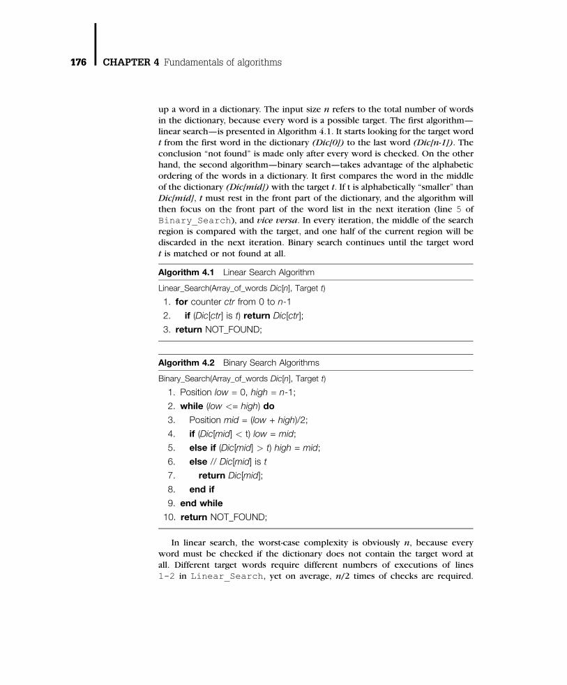
up a word in a dictionary. The input size n refers to the total number of words

in the dictionary, because every word is a possible target. The first algorithm—linear search—is presented in Algorithm 4.1. It starts looking for the target word

t from the first word in the dictionary (Dic[0]) to the last word (Dic[n-1]). The

conclusion “not found” is made only after every word is checked. On the other

hand, the second algorithm—binary search—takes advantage of the alphabetic

ordering of the words in a dictionary. It first compares the word in the middle

of the dictionary (Dic[mid]) with the target t. If t is alphabetically “smaller” than

Dic[mid], t must rest in the front part of the dictionary, and the algorithm will

then focus on the front part of the word list in the next iteration (line 5 ofBinary_Search), and vice versa. In every iteration, the middle of the search

region is compared with the target, and one half of the current region will be

discarded in the next iteration. Binary search continues until the target word

t is matched or not found at all.

Algorithm 4.1 Linear Search Algorithm

Linear_Search(Array_of_words Dic[n], Target t)

1. for counter ctr from 0 to n-1

2. if (Dic[ctr] is t) return Dic[ctr];

3. return NOT_FOUND;

Algorithm 4.2 Binary Search Algorithms

Binary_Search(Array_of_words Dic[n], Target t)

1. Position low = 0, high = n-1;

2. while (low <= high) do

3. Position mid = (low + high)/2;

4. if (Dic[mid] < t) low = mid;

5. else if (Dic[mid] > t) high = mid;

6. else // Dic[mid] is t

7. return Dic[mid];

8. end if

9. end while

10. return NOT_FOUND;

In linear search, the worst-case complexity is obviously n, because every

word must be checked if the dictionary does not contain the target word at

all. Different target words require different numbers of executions of lines

1-2 in Linear_Search, yet on average, n/2 times of checks are required.


Thus, the average-case complexity is roughly n/2. Binary search is apparently

quicker than linear search. Because in every iteration of the while loop inBinary_Search one-half of the current search area is discarded, at most

log2 n (simplified as lg n in the computer science community) of lookups are

required—the worst-case complexity. n is clearly larger than lg n, which proves

that binary search is a more efficient algorithm. Its average-case complexity can

be calculated as in Equation (4.1) by adding up all the possible numbers of

executions and dividing the result by n.

average� case� complexity ¼ 1�1þ 2�2þ 4�3þ 8�4þ . . .þ n

2�lg n

0@

1A=n

¼ lg n� 1þ 3

n

ð4:1Þ

4.2.1 Asymptotic notations

In computational complexity theory, not all parts of an algorithm’s running time

are essential. In fact, only the rate of growth or the order of growth of the run-

ning time is typically of most concern in comparing the complexities of different

algorithms. For example, consider two algorithms A and B, where A has longer run-

ning time for smaller input sizes, and Bhas a higher rate of growth of running time as

the input size increases. Obviously, the running time of B will outnumber that of

A for input sizes greater than a certain number. As in real applications, the input sizeof aproblem is typically very large, algorithmBwill always runmore slowly, and thus

we will consider it as the one with higher computational complexity.

Similarly, it is also sufficient to describe the complexity of an algorithm con-

sidering only the factor that has highest rate of growth of running time. That is,

if the computational complexity of an algorithm is formulated as an equation,

we can then focus only on its dominating term, because other lower-order

terms are relatively insignificant for a large n. For example, the average-case

complexity of Binary_Search, which was shown in Equation (4.1), can besimplified to only lg n, leaving out the terms �1 and 3/n. Furthermore, we

can also ignore the dominating term’s constant coefficient, because it contrib-

utes little information for evaluating an algorithm’s efficiency. In the example

of Linear_Search in Algorithm 4.1, its worst-case complexity and average-

case complexity—n and n/2, respectively—are virtually equal under this crite-

rion. In other words, they are said to have asymptotically equal complexity for

larger n and are usually represented with the following asymptotic notations.

Asymptotic notations are symbols used in computational complexity the-ory to express the efficiency of algorithms with a focus on their orders of growth.

The three most used notations are O-notation, O-notation, and Y-notation.


4.2.1.1 O-notation

O-notation is the dominant method used to express the complexity of algo-

rithms. It denotes the asymptotic upper bounds of the complexity functions.

For a given function g(n), the expression O(g(n)) (read as “big-oh of g of n”)

represents the set of functions

OðgðnÞÞ ¼ ff ðnÞ: positive constants c and n0 exist such that

0 � f ðnÞ � cgðnÞ for all n � n0gA non-negative function f(n) belongs to the set of functions O(g(n)) if there is a

positive constant c that makes f(n) � cg(n) for a sufficiently large n. We can

write f(n) 2 O(g(n)) because O(g(n)) is a set, but it is conventionally written

as f(n) ¼ O(g(n)). Readers have to be careful to note that the equality signdenotes set memberships in all kinds of asymptotic notations.

The definition of O-notation explains why lower-order terms and constant

coefficients of leading terms can be ignored in complexity theory. The following

are examples of legal expressions in computational theory:

n2 ¼ Oðn2Þn3 þ 1000n2 þ n ¼ Oðn3Þ

1000n ¼ OðnÞ20n3 ¼ Oð0:5n3 þ n2Þ

Figure 4.2 shows the most frequently used O-notations, their names, and the

comparisons of actual running times with different values of n. The first order

of functions, O(1), or constant time complexity, signifies that the algorithm’s

running time is independent of the input size and is the most efficient. Theother O-notations are listed in their rank order of efficiency. An algorithm can

be considered feasible with quadratic time complexity O(n2) for a relatively

small n, but when n ¼ 1,000,000, a quadratic-time algorithm takes dozens of

Also called n = 100 n = 10,000 n = 1,000,000 O(1) 0.000001 sec.

O(lg n)O(n)

O(nlg n)O(n2)O(n3)O(2n) O(n!)

Constant time 0.000001 sec.0.000001 sec.0.00002 sec.0.000013 sec.0.000007 sec.Logarithmic time

1 sec.0.01 sec.0.0001 sec.Linear time20 sec.0.13 sec.0.00066 sec.

278 hours100 sec.0.01 sec.Quadratic time317 centuries278 hours1 sec.Cubic time

1030087centuries102995 centuries1014 centuriesExponential timeN/A1035645 centuries10143 centuriesFactorial time

FIGURE 4.2

Frequently used orders of functions and their aliases, along with their actual running time

on a million-instructions-per-second machine with three input sizes: n ¼ 100, 10,000, and

1,000,000.


days to complete the task. An algorithm with a cubic time complexity may han-

dle a problem with small-sized inputs, whereas an algorithm with exponentialor factorial time complexity is virtually infeasible. If an algorithm’s time com-

plexity can be expressed with or is asymptotically bounded by a polynomial

function, it has polynomial time complexity. Otherwise, it has exponentialtime complexity. These will be further discussed in Subsection 4.2.2.

4.2.1.2 O-notation and Q-notation

O-notation is the inverse of O-notation. It is used to express the asymptoticlower bounds of complexity functions. For a given function g(n), the expres-

sion O( g(n)) (read as “big-omega of g of n”) denotes the set of functions:

O ðgðnÞÞ ¼ ff ðnÞ: positive constants c and n0 exist such that

0 � cgðnÞ � f ðnÞ for all n � n0gFrom the definitions of O- and O-notation, the following mutual relationship

holds:

f ðnÞ ¼ OðgðnÞÞ if and only if gðnÞ ¼ O ðf ðnÞÞ

O-notation receives much less attention than O-notation, because we are usu-

ally concerned about how much time at most would be spent executing an

algorithm instead of the least amount of time spent.

Y-notation expresses the asymptotically tight bounds of complexity func-

tions. Given a function g(n), the expression Y(g(n)) (read as “big-theta of g ofn”) denotes the set of functions

YðgðnÞÞ ¼ f f ðnÞ: positive constants c1; c2; and n0 exist such that

0 � c1gðnÞ � f ðnÞ � c2gðnÞ for all n � n0gA function f(n) can be written as f(n) ¼ Y(g(n)) if there are positive coefficients

c1 and c2 such that f(n) can be squeezed between c1g(n) and c2g(n) for a suffi-

ciently large n. Comparing the definitions of all three asymptotic notations, the

following relationship holds:

f ðnÞ ¼ YðgðnÞÞ if and only if f ðnÞ ¼ OðgðnÞÞ and f ðnÞ ¼ OðgðnÞÞIn effect, this powerful relationship is often exploited for verifying theasymptotically tight bounds of functions [Knuth 1976].

Although Y-notation is more precise when characterizing algorithm com-

plexity, O-notation is favored over Y-notation for the following two reasons:

(1) upper bounds are considered sufficient for characterizing algorithm com-

plexity, and (2) it is often much more difficult to prove a tight bound than it

is to prove an upper bound. In the remainder of the text, we will stick with

the convention and use O-notation to express algorithm complexity.


4.2.2 Complexity classes

In the previous subsection, complexity was shown to characterize the efficiencyof algorithms. In fact, complexity can also be used to characterize the problems

themselves. A problem’s complexity is equivalent to the time complexity of the

most efficient possible algorithm. For instance, the dictionary lookup problem

mentioned in the introduction of Section 4.2 has a complexity of O(lg n), the

complexity of Binary_Search in Algorithm 4.2.

To facilitate the exploration and discussion of the complexities of various

problems, those problems that share the same degree of complexity are

grouped, forming complexity classes. Many complexity classes have been estab-lished in the history of computer science [Baase 1978], but in this subsection

we will only discuss those that pertain to problems in the EDA applications.

We will make the distinction between optimization and decision problems first,

because these are key concepts within the area of complexity classes. Then,

four fundamental and important complexity classes will be presented to help

readers better understand the difficult problems encountered in the EDA

applications.

4.2.2.1 Decision problems versus optimization problems

Problems can be categorized into two groups according to the forms of their

answers: decision problems and optimization problems. Decision problemsask for a “yes” or “no” answer. The dictionary lookup problem, for example,

is a decision problem, because the answer could only be whether the target is

found or not. On the other hand, an optimization problem seeks for an opti-

mized value of a target variable. For example, in a combinational circuit, a criti-

cal path is a path from an input to an output in which the sum of the gate and

wire delays along the path is the largest. Finding a critical path in a circuit is an

optimization problem. In this example, optimization means the maximization

of the target variable. However, optimization can also be minimization in othertypes of optimization problems.

An example of a simple decision problem is the HAMILTONIAN CYCLE prob-

lem. The names of decision problems are conventionally given in all capital let-

ters [Cormen 2001]. Given a set of nodes and a set of lines such that each line

connects two nodes, a HAMILTONIAN CYCLE is a loop that goes through all the

nodes without visiting any node twice. The HAMILTONIAN CYCLE problem

asks whether such a cycle exists for a given graph that consists of a set of nodes

and lines. Figure 4.3 gives an example in which a Hamiltonian cycle exists.A famous optimization problem is the traveling salesman problem (TSP). As

its name suggests, TSP aims at finding the shortest route for a salesman who

needs to visit a certain number of cities in a round tour. Figure 4.4 gives a sim-

ple example of a TSP. There is also a version of the TSP as a decision problem:

TRAVELING SALESMAN asks whether a route with length under a constant k

exists. The optimization version of TSP is more difficult to solve than its


decision version, because if the former is solved, the latter can be immediatelyanswered for any constant k. In fact, an optimization problem usually can be

decomposed into a series of decision problems by use of a different constant

as the target for each decision subproblem to search for the optimal solution.

Consequently, the optimization version of a problem always has a complexity

equal to or greater than that of its decision version.

4.2.2.2 The complexity classes P versus NP

The complexity class P, which stands for polynomial, consists of problems that

can be solved with known polynomial-time algorithms. In other words, for any

problem in the class P, an algorithm of time complexity O(nk) exists, where k is

a constant. The dictionary lookup problem mentioned in Section 4.2 lies in P,

because Linear_Search in Algorithm 4.1 has a complexity of O(n).

The nondeterministic polynomial or NP complexity class involves the concept

of a nondeterministic computer, so wewill explain this idea first. A nondeterminis-

tic computer is not a device that can be created from physical components but is aconceptual tool that only exists in complexity theory. A deterministic computer, or

an ordinary computer, solves problems with deterministic algorithms. The charac-

terization of determinism as applied to an algorithm means that at any point in

the process of computation the next step is always determined or uniquely defined

by the algorithm and the inputs. In other words, given certain inputs and a deter-

ministic computer, the result is always the samenomatter howmany times the com-

puter executes the algorithm. By contrast, in a nondeterministic computer multiple

(a) (b) (c)

FIGURE 4.4

(a) An example of the traveling salesman problem, with dots representing cities.

(b) A non-optimal solution. (c) An optimal solution.

FIGURE 4.3

A graph with one HAMILTONIAN CYCLE marked with thickened lines.


possibilities for the next step are available at each point in the computation, and

the computer will make a nondeterministic choice from these possibilities, whichwill somehow magically lead to the desired answer. Another way to understand

the idea of a nondeterministic computer is that it can execute all possible options

in parallel at a certain point in the process of computation, compare them, and then

choose the optimal one before continuing.

Problems in the NP complexity class have three properties:

1. They are decision problems.

2. They can be solved in polynomial time on a nondeterministic computer.

3. Their solution can be verified for correctness in polynomial time on a

deterministic computer.

The TRAVELING SALESMAN decision problem satisfies the first two of these

properties. It also satisfies the third property, because the length of the solution

route can be calculated to verify whether it is under the target constant k in

linear time with respect to the number of cities. TRAVELING SALESMAN is,

therefore, an NP class problem. Following the same reasoning process, HAMIL-

TONIAN CYCLE is also in this class.A problem that can be solved in polynomial time by use of a deterministic

computer can also definitely be solved in polynomial time on a nondeterminis-

tic computer. Thus, P � NP. However, the question of whether NP ¼ P remains

unresolved—no one has yet been able to prove or disprove it. To facilitate this

proof (or disproof), the most difficult problems in the class NP are grouped

together as another complexity class, NP-complete; proving P ¼ NP is equiva-

lent to proving P ¼ NP-complete.

4.2.2.3 The complexity class NP-complete

Informally speaking, the complexity class NP-complete (or NPC) consists of the

most difficult problems in the NP class. Formally speaking, for an arbitrary prob-

lem Pa in NP and any problem Pb in the class NPC, a polynomial transforma-

tion that is able to transform an example of Pa into an example of Pb exists.

A polynomial transformation can be defined as follows: given two problemsPa and Pb, a transformation (or reduction) from Pa to Pb can express any exam-

ple of Pa as an example of Pb. Then, the transformed example of Pb can be

solved by an algorithm for Pb, and its answer can then be mapped back to an

answer to the problem of Pa. A polynomial transformation is a transformation

with a polynomial time complexity. If a polynomial transformation from Pa to

Pb exists, we say that Pa is polynomially reducible to Pb. Now we illustrate this

idea by showing that the decision problem HAMILTONIAN CYCLE is polynomi-

ally reducible to another decision problem—TRAVELING SALESMAN.Given a graph consisting of n nodes and m lines, with each line connecting

two nodes among the n nodes, a HAMILTONIAN CYCLE consists of n lines that

traverse all n nodes, as in the example of Figure 4.3. This HAMILTONIAN CYCLE

problem can be transformed into a TRAVELING SALESMAN problem by assigning


a distance to each pair of nodes. We assign a distance of 1 to each pair of nodes

with a line connecting them. For the rest of node pairs, we assign a distancegreater than 1, say, 2. With such assignments, the TRAVELING SALESMAN prob-

lem of finding whether a round tour of a total distance not greater than n exists

is equal to finding a HAMILTONIAN CYCLE in the original graph. If such a tour

exists, the total length of the route must be exactly n, and all the distances

between the neighboring cities on the route must be 1, which corresponds to

existing lines in the original graph; thus, a HAMILTONIAN CYCLE is found. This

transformation from HAMILTONIAN CYCLE to TRAVELING SALESMAN is merely

based on the assignments of distances, which are of polynomial time complex-ity—or, more precisely, quadratic time complexity—with respect to the number

of nodes. Therefore the transformation is a polynomial transformation.

Now that we understand the concept of a polynomial transformation, we

can continue discussing NP-completeness in further detail. Any problem in

NPC should be polynomially reducible from any NP problem. Do we need to

examine all NP problems if a polynomial transformation exists? In fact, a prop-

erty of the NPC class can greatly simplify the proof of the NP-completeness of a

problem: all problems in the class NPC are polynomially reducible to oneanother. Consequently, to prove that a problem Pt is indeed NPC, only two

properties have to be checked:

1. The problem Pt is an NP problem, that is, Pt can be solved in polynomialtime on a nondeterministic computer. This is also equivalent to showing

that the solution checking of Pt can be done in polynomial time on a

deterministic computer.

2. A problem already known to be NP-complete is polynomially reducible to

the target problem Pt.

For example, we know that HAMILTONIAN CYCLE is polynomially reducible to

TRAVELING SALESMAN. Because the former problem is an NPC problem, and

TRAVELING SALESMAN is an NP problem, TRAVELING SALESMAN is, therefore,

proven to be contained in the class of NPC.

Use of transformations to prove a problem to be in the NPC class relies on

the assumption that there are already problems known to be NP-complete.

Hence, this kind of proof is justified only if there is one problem proven to beNP-complete in another way. Such a problem is the SATISFIABILITY problem.

The input of this problem is a Boolean expression in the product of sums form

such as the following example: x1 þ x2 þ x3ð Þ x2 þ x4ð Þ x1 þ x3ð Þ x2 þ x3 þ x4ð Þ.The problem aims at assigning a Boolean value to each of the input variables

xi so that the overall product becomes true. If a solution exists, the expression

is said to be satisfiable. Because the answer to the problem can only be true or

false, SATISFIABILITY, or SAT, is a decision problem.

The NP-completeness of the SAT problem is proved with Cook’s theorem

[Cormen 2001] by showing that all NP problems can be polynomially reduced

to the SAT problem. The formal proof is beyond the scope of this book [Garey


1979], so we will only informally demonstrate its concept. We have mentioned

that all NP problems can be solved in polynomial time on a nondeterministic

computer. For an arbitrary NP problem, if we record all the steps taken on a

nondeterministic computer to solve the problem in a series of statements,

Cook’s theorem proves that the series of statements can be polynomially trans-

formed into a product of sums, which is in the form of an SAT problem. As aresult, all NP problems can be polynomially reduced to the SAT problem; conse-

quently, the SAT problem is NP-complete.

An open question in computer science is whether a problem that lies in both

the P and the NPC classes exists. No one has been able to find a deterministic

algorithm with a polynomial time complexity that solves any of the NP-

complete problems. If such an algorithm can be found, all of the problems in

NPC can be solved by that algorithm in polynomial time, because they are poly-

nomially reducible to one another. According to the definition of NP-complete-ness, such an algorithm can also solve all problems in NP, making P ¼ NP, as

shown in Figure 4.5b. Likewise, no one has been able to prove that for any of

the problems in NPC no polynomial time algorithm exists. As a result, although

the common belief is that P 6¼ NP, as shown in Figure 4.5a, and decades of

endeavors to tackle NP-complete problems suggest this is true, no hard

evidence is available to support this point of view.

4.2.2.4 The complexity class NP-hard

Although NP-complete problems are realistically very difficult to solve, there are

other problems that are even more difficult: NP-hard problems. The NP-hard

complexity class consists of those problems at least as difficult to solve as NP-complete problems. A specific way to define an NP-hard problem is that the

solution checking for an NP-hard problem cannot be completed in polynomial

time. In practice, many optimization versions of the decision problems in NPC

are NP-hard. For example, consider the NP-complete TRAVELING SALESMAN

problem. Its optimization version, TSP, searches for a round tour going through

all cities with a minimum total length. Because its solution checking requires

computation of the lengths of all possible routes, which is a O(n � n!) procedure,with n being the number of cities, the solution definitely cannot be found in

NPCP

NP

(a) (b)

All problems

P = NP = NPC

All problems

P ≠ NP P = NP

FIGURE 4.5

Relationship of complexity classes if (a) P 6¼ NP or (b) P ¼ NP.


polynomial time. Therefore, TSP, an optimization problem, belongs to the NP-hard class.

4.3 GRAPH ALGORITHMSA graph is a mathematical structure that models pairwise relationships among

items of a certain form. The abstraction of graphs often greatly simplifies

the formulation, analysis, and solution of a problem. Graph representationsare frequently used in the field of Electronic Design Automation. For example,

a combinational circuit can be efficiently modeled as a directed graph to

facilitate structure analysis, as shown in Figure 4.6.

Graph algorithms are algorithms that exploit specific properties in various

types of graphs [Even 1979; Gibbons 1985]. Given that many problems in the

EDA field can be modeled as graphs, efficient graph algorithms can be directly

applied or slightly modified to address them. In this section, the terminology

and data structures of graphs will first be introduced. Then, some of the most fre-quently used graph algorithms will be presented.

4.3.1 Terminology

A graph G is defined by two sets: a vertex set V and an edge set E. Customarily, a

graph is denoted with G(V, E). Vertices can also be called nodes, and edges can

be called arcs or branches. In this chapter, we use the terms vertices and edges.

Figure 4.7 presents a graph G with V ¼ {v1, v2, v3, v4, v5} and E ¼ {e1, e2, e3,e4, e5}. The two vertices connected by an edge are called the edge’s endpoints.

An edge can also be characterized by its two endpoints, u and v, and denoted as

(u, v). In the example of Figure 4.7, e1 ¼ (v1, v2), e2 ¼ (v2, v3), etc. If there is an

edge e connecting u and v, the two vertices u and v are adjacent and edge e is

v1

v3

v2 v4

v5

e1

e2 e3

e4

e5

FIGURE 4.7

An exemplar graph.

AB

C

DE

A

BC

DE

FIGURE 4.6

A combinational circuit and its graph representation.

4.3 Graph algorithms 185

incident with u (and also with v). The degree of a vertex is equal to the number

of edges incident with it.

A loop is an edge that starts and ends at the same vertex. If plural edges are

incident with the same two vertices, they are called parallel edges. A graph

without loops and parallel edges is called a simple graph. In most discussions

of graphs, only simple graphs are considered, and, thus, a graph implicitlymeans a simple graph. A graph without loops but with parallel edges is known

as a multigraph.

The number of vertices in a graph is referred to as the order of the graph, or

simply jV j. Similarly, the size of a graph, denoted as jE j, refers to its number of

edges. It is worth noting that inside asymptotic notations, such as O and Y, and

only inside them, jV j and jE j can be simplified as V and E. For example, O(jV j þjE j) can be expressed as O(V þ E).

A path in a graph is a sequence of alternating vertices and edges such thatfor each vertex and its next vertex in the sequence, the edge between these ver-

tices connects them. The length of a path is defined as the number of edges in a

path. For example, in Figure 4.7, <v5, e4, v3, e3, v4> is a path with a length of

two. A path in which the first and the last vertices are the same is called a cycle.

<v5, e4, v3, e3, v4, e5, v5> is a cycle in Figure 4.7. A path, in which every vertex

appears once in the sequence is called a simple path. The word “simple” is

often omitted when this term is used, because we are only interested in simple

paths most of the time.The terms defined so far are for undirected graphs. In the following, we

introduce the terminology for directed graphs. In a directed graph, every edge

has a direction. We typically use arrows to represent directed edges as shown

in the examples in Figure 4.8. For an edge e ¼ (u, v) in a directed graph, u

and v cannot be freely exchanged. The edge e is directed from u to v, or equiv-

alently, incident from u and incident to v. The vertex u is the tail of the edge e;

v is the head of the edge e. The degree of a vertex in a directed graph is divided

into the in-degree and the out-degree. The in-degree of a vertex is the numberof edges incident to it, whereas the out-degree of a vertex is the number of

edges incident from it. For the example of G2 in Figure 4.8, the in-degree of

v2 is 2 and its out-degree is 1.

The definitions of paths and cycles need to be revised as well for a directed

graph: every edge in a path or a cycle must be preceded by its tail and followed

by its head. For example, <v4, e4, v2, e2, v3> in G1 of Figure 4.8 is a path and

<v1, e1, v2, e2, v3, e3, v1> is a cycle, but <v4, e4, v2, e1, v1> is not a path.

v1v2

v3

v5v4

v3v2

v5v4

v1e1

e3

e2

e4

e5

e1

e2e3

e4

e5

G1: G2:

FIGURE 4.8

Two examples of directed graphs.


If a vertex u appears before another vertex v in a path, u is v’s predecessor on

that path and v is u’s successor. Notice that there is no cycle in G2. Suchdirected graphs without cycles are called directed acyclic graphs or DAGs.

DAGs are powerful tools used to model combinational circuits, and we will

dig deeper into their properties in the following subsections.

In some applications, we can assign values to the edges so that a graph can

convey more information related to the edges other than their connections. The

values assigned to edges are called their weights. A graph with weights assigned

to edges is called a weighted graph. For example, in a DAG modeling of a com-

binational circuit, we can use weights to represent the time delay to propagate asignal from the input to the output of a logic gate. By doing so, critical paths can

be conveniently determined by standard graph algorithms.

4.3.2 Data structures for representations of graphs

Several data structures are available to represent a graph in a computer, but

none of them is categorically better than the others [Aho 1983; Tarjan 1987].

They all have their own advantages and disadvantages. The choice of the datastructure depends on the algorithm [Hopcroft 1973].

The simplest data structure for a graph is an adjacency matrix. For a graph

G ¼ (V, E), a jV j � jV j matrix A is needed. Aij ¼ 1 if (vi, vj) 2 E, and Aij ¼ 0 if (vi,

vj) =2 E. For an undirected graph, the adjacency matrix is symmetrical, because

the edges have no directions. Figure 4.9 shows the adjacency matrices for the

graph in Figure 4.7 and G2 in Figure 4.8.

One of the strengths of the use of an adjacency matrix is that it can easily repre-

sent a weighted graph by changing the ones in the matrix to the edges’ respectiveweights. However, the weight cannot be a zero in this representation (otherwise

we cannot differentiate zero-weight edge from “no connection” between two verti-

ces). Also, an adjacency matrix requires exactlyY(V 2) space. For a dense graph for

which jE j is close to jV j2, this couldbe amemory-efficient representation.However,

if the graph is sparse, that is, jE j is much smaller than jV j2, most of the entries in the

adjacency matrix would be zeros, resulting in a waste of memory.

A sparse graph is better represented with an adjacency list, which consists

of an array of size jV j, with the ith element corresponding to the vertex vi.The ith element points to a linked list that stores those vertices adjacent to vi

00000

10010

00001

00100

00010

(a) (b)

01100

10100

11010

00101

00010

FIGURE 4.9

The adjacency matrices: (a) for Figure 4.7. (b) for G2 in Figure 4.8.


in an undirected graph. For a directed graph, any vertex vj in the linked list ofthe ith element satisfies the condition (vi, vj) 2 E. The adjacency list for G1 in

Figure 4.8 is shown in Figure 4.10.

4.3.3 Breadth-first search and depth-first search

Many graph algorithms rely on efficient and systematic traversals of vertices and

edges in the graph. The two simplest and most commonly used traversal meth-

ods are breadth-first search and depth-first search, which form the basis for

many graph algorithms. We will examine their generic structures and pointout some important applications.

4.3.3.1 Breadth-first search

Breadth-first search (BFS) is a systematic means of visiting vertices and edges in

a graph. Given a graph G and a specific source vertex s, the BFS searches

through those vertices adjacent to s, then searches the vertices adjacent tothose vertices, and so on. The routine stops when BFS has visited all vertices

that are reachable from s. The phenomenon that the vertices closest to the

source s are visited earlier in the search process gives this search its name. Sev-

eral procedures can be executed when visiting a vertex. The function BFS in

Algorithm 4.3 adopts two of the most frequently used procedures: building a

breadth-first tree and calculating the distance, which is the minimum length

of a path, from the source s to each reachable vertex.

Algorithm 4.3 Breadth-first Search Algorithm

BFS (Graph G, Vertex s)

1. FIFO_Queue Q = {s};

2. for (each v 2 V) do

3. v.visited = false; // visited by BFS

4. v.distance = 1; // distance from source s

5. v.predecessor = NIL; // predecessor of v

6. end for

7. s.visited = true;

1

2

3

4

5

2

3

1

2 5

FIGURE 4.10

The adjacency list for G1 of Figure 4.8.


8. s.distance = 0;

9. while (Q 6¼ �) do

10. Vertex u = Dequeue(Q);

11. for (each (u, w) 2 E) do

12. if (!(w.visited))

13. w.visited = true;

14. w.distance = u.distance + 1;

15. w.predecessor = u;

16. Enqueue(Q, w);

17. end if

18. end for

19. end while

The function BFS implements breadth-first search with a queue Q. The

queue Q stores the indices of, or the links to, the visited vertices whose adjacent

vertices have not yet been examined. The first-in first-out (FIFO) property of aqueue guarantees that BFS visits every reachable vertex once, and all of its adja-

cent vertices are explored in a breadth-first fashion. Because each vertex and

edge is visited at most once, the time complexity of a generic BFS algorithm is

O(V þ E), assuming the graph is represented by an adjacency list.

Figure 4.11 shows a graph produced by the BFS in Algorithm 4.3 that also

indicates a breadth-first tree rooted at v1 and the distances of each vertex to v1.

The distances of v7 and v8 are infinity, which indicates that they are disconnected

from v1. In contrast, subsets of a graph in which the vertices are connected toone another and to which no additional vertices are connected, such as the set

from v1 to v6 in Figure 4.11, are called connected components of the graph.

One of the applications of BFS is to find the connected components of a graph.

The attributes distance and predecessors indicate the lengths and the

routes of the shortest paths from each vertex to the vertex v1. A BFS algorithm

v1 v3 v7v5

v6v4v2 v8 v2 v4 v6 v8

v1 v3 v5 v7

0 0 3 4

321

�

�

�

�

�

�

�

��

FIGURE 4.11

Applying BFS on an undirected graph with source v1. The left is the graph after line 8 and the

right shows the graph after the completion of the BFS. Numbers in the vertices are their

distances to the source v1. Thick edges are breadth-first tree edges.


can also compute the shortest paths and their lengths from a source vertex to all

other vertices in an unweighted graph. The calculation of the shortest paths in aweighted graph will be discussed in Subsection 4.3.6.

4.3.3.2 Depth-first search

While BFS traverses a graph in a breadth-first fashion, depth-first search (DFS)

explores the graph in an opposite manner. From a predetermined source vertex

s, DFS traverses the vertex as deep as possible along a path before backtracking,

just as the name implies. The recursive function DFSPrototype, shown in

Algorithm 4.4, is the basic structure for a DFS algorithm.

Algorithm 4.4 A Prototype of the Depth-first Search Algorithm

DFSPrototype(Vertex v)

1. // Pre-order process on v;

2. mark v as visited;

3. for (each unvisited vertex u adjacent to v)

4. DFSPrototype(u);

5. // In-order process on v;

6. end for

7. // Post-order process on v

The terms pre-order, in-order, and post-order processes on the lines 1, 5,

and 7 in Algorithm 4.4 refer to the traversal patterns on a conceptual tree

formed by all the vertices in the graph. DFS performs a pre-order process onall the vertices in the exact same order as a pre-order tree traversal in the result-

ing “depth-first forest.” This is also the case for in-order and post-order pro-

cesses. The functionality of these processes, which will be tailor-designed to

an application, is the basis of DFS algorithms. The function DFS in Algorithm

4.5 provides an example of a post-order process.

Algorithm 4.5 A Complete Depth-first Search Algorithm

DFS(Graph G)

1. for (each vertex v 2 V) do

2. v.visited = false;

3. v.predecessor = NIL;

4. end for

5. time = 0;

6. for (each vertex v 2 V)

7. if (!(v.visited))

8. DFSVisit(v);


9. end if

10. end for

DFSVisit(Vertex v)

1. v.visited = true;

2. for (each (v, u) 2 E)

3. if (!(u.visited)) do

4. u.predecessor = v;

5. DFSVisit(u);

6. end if

7. end for

8. time = time + 1;

9. v.PostOrderTime = time;

Notice that it is guaranteed that every vertex will be visited by lines 6 and 7

in DFS. This is another difference between DFS and BFS. For most applicationsof DFS, it is preferred that all vertices in the graph be visited. As a result, a

depth-first forest is formed instead of a tree. Moreover, because each vertex

and edge is explored exactly once, the time complexity of a generic DFS

algorithm is O(V þ E) assuming the use of an adjacency list.

Figure 4.12 demonstrates a directed graph on which DFS(G1) is executed.

The PostOrderTimes of all vertices and the tree edges of a depth-first forest,

which is constructed from the predecessor of each vertex, are produced as

the output. PostOrderTimes have several useful properties. For example, thevertices with a lower post-order time are never predecessors of those with a

higher post-order time on any path. The next subsection uses this property

for sorting the vertices of a DAG. In Subsection 4.3.5, we will introduce some

important applications of the depth-first forest.

6 4 8

735

9 2 1

v1 v2 v3

v4 v5 v6

v7 v8 v9

v1 v2 v3

v4 v5 v6

v7 v8 v9

Unvisited: All visited:

FIGURE 4.12

Applying DFS on a directed graph G1. The numbers in the vertices are their

PostOrderTimes. Thickened edges show how a depth-first forest is built.


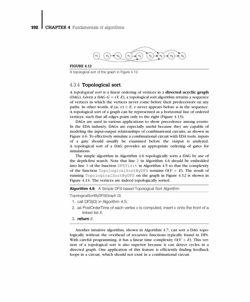
4.3.4 Topological sort

A topological sort is a linear ordering of vertices in a directed acyclic graph(DAG). Given a DAG G ¼ (V, E), a topological sort algorithm returns a sequence

of vertices in which the vertices never come before their predecessors on any

paths. In other words, if (u, v) 2 E, v never appears before u in the sequence.

A topological sort of a graph can be represented as a horizontal line of ordered

vertices, such that all edges point only to the right (Figure 4.13).DAGs are used in various applications to show precedence among events.

In the EDA industry, DAGs are especially useful because they are capable of

modeling the input-output relationships of combinational circuits, as shown in

Figure 4.6. To effectively simulate a combinational circuit with EDA tools, inputs

of a gate should usually be examined before the output is analyzed.

A topological sort of a DAG provides an appropriate ordering of gates for

simulations.

The simple algorithm in Algorithm 4.6 topologically sorts a DAG by use ofthe depth-first search. Note that line 2 in Algorithm 4.6 should be embedded

into line 9 of the function DFSVisit in Algorithm 4.5 so that the complexity

of the function TopologicalSortByDFS remains O(V þ E). The result of

running TopologicalSortByDFS on the graph in Figure 4.12 is shown in

Figure 4.13. The vertices are indeed topologically sorted.

Algorithm 4.6 A Simple DFS-based Topological Sort Algorithm

TopologicalSortByDFS(Graph G)

1. call DFS(G) in Algorithm 4.5;

2. as PostOrderTime of each vertex v is computed, insert v onto the front of alinked list ll;

3. return ll;

Another intuitive algorithm, shown in Algorithm 4.7, can sort a DAG topo-

logically without the overhead of recursive functions typically found in DFS.

With careful programming, it has a linear time complexity O(V þ E). This ver-

sion of a topological sort is also superior because it can detect cycles in a

directed graph. One application of this feature is efficiently finding feedback

loops in a circuit, which should not exist in a combinational circuit.

v7 v3 v6 v1 v4 v2 v5 v8 v9

FIGURE 4.13

A topological sort of the graph in Figure 4.12.


Algorithm 4.7 A Topological Sort Algorithm that can Detect Cycles

TopologicalSort(Graph G)

1. FIFO_Queue Q = {vertices with in-degree 0};

2. LinkedList ll = �;

3. while (Q is not empty) do

4. Vertex v = Dequeue(Q);

5. insert v into ll;

6. for (each vertex u such that (v, u) 2 E) do

7. remove (v, u) from E;

8. if (in-degree of u is 0) Enqueue(Q, u);

9. end for

10. end while

11. if (E 6¼ �) return “G has cycles”;

12. else return ll;

4.3.5 Strongly connected component

A connected component in an undirected graph has been defined in Subsection

4.3.3.1. For a directed graph, connectivity is further classified into “strong con-

nectivity” and “weak connectivity.” A directed graph is weakly connected if all

vertices are connected provided all directed edges are replaced as undirected

edges. For a strongly connected directed graph, every vertex must be reachablefrom every other vertex. More precisely, for any two vertices u and v in a

strongly connected graph, there exists a path from u to v, as well as a path from

v to u. A strongly connected component (SCC) in a directed graph is a subset of

the graph that is strongly connected and is maximal in the sense that no addi-

tional vertices can be included in this subset while still maintaining the property

of strong connectivity. Figure 4.14a shows a weakly connected graph with four

strongly connected components. As an SCC consisting of more than one vertex

must contain cycles, it follows naturally that a directed acyclic graph has noSCCs that consist of more than one vertex.

The algorithm used to extract SCCs, SCC in Algorithm 4.8, requires the

knowledge of the transpose of a directed graph (line 2). A transpose of a

directed graph G, GT, contains the same vertices of G, but the directed edges

are reversed. Formally speaking, for G ¼ (V, E), GT ¼ (V, ET) with ET ¼ {(u,

v): (v, u) 2 E}. Transposing a graph incurs a linear time complexity O(V þ E),

which preserves the efficiency of the algorithm for finding SCCs.


Algorithm 4.8 An Algorithm to Extract SCCs from a Directed Graph

SCC(Graph G)

1. call DFS(G) in Algorithm 4.5 for PostOrderTime;

2. GT = transpose(G);

3. call DFS(GT), replacing line 6 of DFS with a procedureexamining vertices in order of decreasing PostOrderTime;

4. return different trees in depth-first forest built in DFS(GT) as separate SCCs;

SCC is simple: a DFS, then a transpose, then another DFS. It is also efficient

because DFS and transpose incur only a linear time complexity, resulting in atime complexity of O(V þ E). Figure 4.14 gives an example of running SCC

on a graph G. The four SCCs are correctly identified by the four depth-first trees

in GT. Moreover, if we view an SCC as a single vertex, the resultant graph,

shown in Figure 4.14, is a DAG. We also observe that examining vertices in a

descending order of the post-order times in DFS is equivalent to visiting the

resultant SCCs in a topologically sorted order.

If we model a sequential circuit as a directed graph where vertices represent

registers and edges represent combinational signal flows between registers,extracting SCCs from the graph identifies clusters of registers, each of which

includes a set of registers with strong functional dependencies among them-

selves. Extracting SCCs also enables us to model each SCC as a single element,

which greatly facilitates circuit analysis because the resultant graph is a DAG.

(a)

9

8

3

v1 v2 v3

v6v5v4

v7 v8 v9

6

25

41

7v1 v2 v3

v6v5v4

v7 v8 v9

(b)

{v1,v2,v4} {v3,v5,v6} {v7,v8} v9

(c)

FIGURE 4.14

(a) A directed graph G after running DFS with depth-first tree edges thickened. Post-order

times are labeled beside each vertex and SCC regions are shaded. (b) The graph GT, the

transpose of G, after running SCC in Algorithm 4.8 (c) Finding SCCs in G as individual

vertices result in a DAG.


4.3.6 Shortest and longest path algorithms

Given a combinational circuit in which each gate has its own delay value, supposewe want to find the critical path—that is, the path with the longest delay—from

an input to an output. A trivial solution is to explicitly evaluate all paths from the

input to the output. However, the number of paths can grow exponentially with

respect to the number of gates. A more efficient solution exists: we can model the

circuit as a directed graph whose edge weights are the delays of the gates. The

longest path algorithm can then give us the answer more efficiently.

In this subsection, we present various shortest and longest path algorithms. Not

only can they calculate the delays of critical paths, but they also can be applied toother EDA problems, such as finding an optimal sequence of state transitions from

the starting state to the target state in a state transition diagram. In the shortest-path

problem or the longest-path problem, we are given a weighted, directed graph.

The weight of a path is defined as the sum of the weights of its constituent edges.

The goal of the shortest-/longest-path problem is to find the path from a source ver-

tex s to a destination vertex d with minimum/maximum weight. Three algorithms

are capable of finding the shortest paths from a source to all other vertices, each

of whichworks on the graphwith different constraints. First, we will present a sim-ple algorithm used to solve the shortest-path problem on DAGs. Dijkstra’s algo-

rithm [Dijkstra 1959], which functions on graphs with non-negative weights, will

then be presented. Finally, we will introduce a more general algorithm that can be

applied to all types of directed graphs—the Bellman-Ford algorithm [Bellman

1958]. On the basis of these algorithms’ concepts, we will demonstrate how to

modify them to apply to longest-path problems.

4.3.6.1 Initialization and relaxation

Before explaining these algorithms, we first introduce two basic techniques

used by all the algorithms in this subsection: initialization and relaxation.

Before running a shortest-path algorithm on a directed graph G ¼ (V, E), wemust be given a source vertex s and the weight of each edge e 2 E, w(e). Also,

two attributes must be stored for each vertex v 2 V: the predecessor pre(v)

and the shortest-path estimate est(v). The predecessor pre(v) records the

predecessor of v on the shortest path, and est(v) is the current estimation of

the weight of the shortest path from s to v. The procedure in Algorithm 4.9,

known as initialization, initializes pre(v) and est(v) for all vertices.

Algorithm 4.9 Initialization Procedure for Shortest-path Algorithms

Initialize(graph G, Vertex s)

1. for (each vertex v 2 V) do

2. pre(v) = NIL; // predecessor

3. est(v) = 1; // shortest-path estimate

4. end for

5. est(s) = 0;


The other common procedure, relaxation, is the kernel of all the algorithms

presented in this subsection. The relaxation of an edge (u, v) is the process ofdetermining whether the shortest path to v found so far can be shortened or

relaxed by taking a path through u. If the shortest path is, indeed, improved

by use of this procedure, pre(v) and est(v) will be updated. Algorithm 4.10

shows this important procedure.

Algorithm 4.10 Relaxation Procedure for Shortest-path Algorithms

Relax(Vertex u, Vertex v)

1. if (est(v) > est(u) + w(u, v)) do

2. est(v) = est(u) + w(u, v));

3. pre(v) = u;

4. end if

4.3.6.2 Shortest path algorithms on directed acyclic graphs

DAGs are always easier to manipulate than the general directed graphs, becausethey have no cycles. By use of a topological sorting procedure, as shown in

Algorithm 4.11, this Y(V þ E) algorithm calculates the shortest paths on a

DAG with respect to a given source vertex s.

The function DAGShortestPaths, used in Algorithm 4.11, sorts the verti-

ces topologically first; in line 4, each vertex is visited in the topologically sorted

order. As each vertex is visited, the function relaxes all edges incident from it.

The shortest paths and their weights are then available in pre(v) and est(v) of

each vertex v. Figure 4.15 gives an example of running DAGShortestPathson a DAG. Notice that the presence of negative weights in a graph does not

affect the correctness of this algorithm.

Algorithm 4.11 A Shortest-path Algorithm for DAGs

DAGShortestPaths(Graph G, vertex s)

1. topologically sort the vertices of G;

2. Initialize(G, s);

3. for (each vertex u in topological sorted order)

4. for (each vertex v such that (u, v) 2 E)

5. Relax(u, v);

6. end for

7. end for

4.3.6.3 Dijkstra’s algorithm

Dijkstra’s algorithm solves the shortest-path problem for any weighted, directed

graph with non-negative weights. It can handle graphs consisting of cycles,


but negative weights will cause this algorithm to produce incorrect results.

Consequently, we assume that w(e) � 0 for all e 2 E here.

The pseudocode in Algorithm 4.12 shows Dijkstra’s algorithm. The algo-

rithm maintains a priority queue minQ that is used to store the unprocessed ver-

tices with their shortest-path estimates est(v) as key values. It then repeatedlyextracts the vertex u which has the minimum est(u) from minQ and relaxes

all edges incident from u to any vertex in minQ. After one vertex is extracted

from minQ and all relaxations through it are completed, the algorithm will treat

this vertex as processed and will not touch it again. Dijkstra’s algorithm stops

either when minQ is empty or when every vertex is examined exactly once.

Algorithm 4.12 Dijkstra’s shortest-path algorithm

Dijkstra(Graph G, Vertex s)


2. Priority_Queue minQ = {all vertices in V};

3. while (minQ 6¼ �) do

4. Vertex u = ExtractMin(minQ); // minimum est(u)

5. for (each v 2 minQ such that (u, v) 2 E)

6. Relax(u, v);

7. end for

8. end while

v0 v1 v2 v3 v4 v54

3

5 -1

-2 7

2

44 7

7777

22222

6666

988

4444

Shortest-Path Estimates Predecessorsvisitedvertex

NIL NIL NILNIL NIL

NIL

v0 v0v0

v0v1

v1 v2 v3 v4 v5 v1 v2 v3 v4 v5

v0 v1v1v1v1

v1v1v1v1v1 v2

v2

v2

v4

v4

v3

v2v0v0v0

∞ 5 ∞ ∞v1 ∞ ∞v2 ∞v3

v5

v4

non NIL NIL NIL NIL NILNIL ∞ ∞ ∞ ∞ ∞

FIGURE 4.15

The upper part is a DAG with its shortest paths shown in thickened edges, and the lower

part is the changes of predecessors and shortest-path estimates when different vertices

are visited in line 3 of the function DAGShortestPaths.


Dijkstra’s algorithm works correctly, because all edge weights are non-negative,

and the vertex with the least shortest-path estimate is always chosen. In the first

iteration of the while loop in lines 3 through 7, the source s is chosen and its

adjacent vertices have their est(v) set tow((s, v)). In the second iteration, the vertex

uwith minimalw((s, u)) will be selected; then those edges incident from uwill be

relaxed. Clearly, there exists no shorter path from s to u than the single edge(s,u), because all weights are not negative, and any path traced that uses an interme-

diate vertex is longer. Continuing this reasoning brings us to the conclusion that the

algorithm, indeed, computes the shortest paths.

Figure 4.16 illustrates the execution of Dijkstra’s algorithm on a directed

graph with non-negative weights and containing cycles. However, a small exam-

ple in Figure 4.17 shows that Dijkstra’s algorithm fails to find the shortest paths

when negative weights exist.

Dijkstra’s algorithm necessitates the use of a priority queue that supports theoperations of extracting a minimum element and decreasing keys. A linear array

can be used, but its complexity will be as much as O(V2 þ E) ¼ O(V2). If a more

(a)

5 9

220

1 64 2

3

v1

v2 v3

v4

v0

(b)

4 2

5 92

201 6

3

v1

v2 v3

v4

v0

(c)

5 92

201 4 2

6

3

v1

v2 v3

v4

v0

00

0 35

333

2222

88

77

55

000

Shortest-Path Estimates Predecessorsvertex

NILv0 v0v2

v0

v0 v1 v2 v3 v4 v0 v1 v2 v3 v4

v2v2v2

v0v0v0v0 v4

v4v1

v1

v1v2

v2 v2

v0 2 ∞ 9v2 6v1 5v4v3

non NILNILNILNILNILNIL

NIL NIL NIL NILNIL ∞ ∞ ∞ ∞

FIGURE 4.16

An example of Dijkstra’s algorithm: (a), (b), and (c) respectively show the edges belonging to

the shortest paths when v0, v2, and v3 are visited. The table exhibits the detailed data when

each vertex is visited.

Predecessors Shortest-Path

Estimatesv0 v1 v2 v0 v1 v2

Dijkstra’s NILNIL

v0 v0 0 2 3Correct path v2 v0 0 1 3

v0

v2v1

2 3

−2

FIGURE 4.17

Running Dijkstra’s algorithm on a graph with negative weights causes incorrect results on v1.


efficient data structure, such as a binary or Fibonacci heap [Moore 1959], is

used to implement the priority queue, the complexity can be reduced.

4.3.6.4 The Bellman-Ford algorithm

Cycles should never appear in a shortest path. However, if there exist negative-weight cycles, a shortest path can have a weight of �1 by circling around

negative-weight cycles infinitely many times. Therefore, negative-weight cycles

should be avoided before finding the shortest paths. In general, we can catego-

rize cycles into three types according to their weights: negative-weight, zero--

weight, and positive-weight cycles. Positive-weight cycles would not appear in

any shortest paths and thus will never be threats. Zero-weight cycles are unwel-

come in most applications, because we generally want a shortest path to have

not only a minimum weight, but also a minimum number of edges.Because a shortest path should not contain cycles, it should traverse every

vertex at most once. It follows that in a directed graph G ¼ (V, E), the maximum

number of edges a shortest path can have is jV j � 1, with all the vertices visited

once. The Bellman-Ford algorithm takes advantage of this observation and

relaxes all the edges (jV j � 1) times. Although this strategy is time-consuming,

with a runtime of O((jV j � 1) � jE j) ¼ O(VE), it helps the algorithm handle

more general cases, such as graphs with negative weights. It also enables the

discovery of negative-weight cycles.The pseudocode of the Bellman-Ford algorithm is shown in Algorithm 4.13.

The negative-weight cycles are detected in lines 5 through 7. They are identi-

fied on the basis of the fact that if any edge can still be relaxed after (jV j � 1)

times of relaxations (line 6), then a shortest path with more than (jV j � 1)

edges exists; therefore, the graph contains negative-weight cycles.

Algorithm 4.13 Bellman-Ford algorithm

Bellman-Ford(Graph G, Vertex s)


2. for (counter = 1 to |V| - 1)

3. for (each edge (u, v) 2 E)

4. Relax(u, v);

5. end for

6. end for

7. for (each edge (u, v) 2 E)

8. if (est(v) > est(u) + w(u, v))

9. report “negative-weight cycles exist”;

10. end if

11. end for


4.3.6.5 The longest-path problem

The longest-path problem can be solved by use of a modified version of the

shortest-path algorithm. We can multiply the weights of the edges by �1

and feed the graph into either the shortest-path algorithm for DAGs or the

Bellman-Ford algorithm. We cannot use Dijkstra’s algorithm, which cannot han-

dle graphs with negative-weight edges. Rather than finding the shortest path,these algorithms discover the longest path. If we do not want to alter any attri-

butes in the graph, we can alter the algorithm by initializing the value of est(v)

to �1 instead of 1, as shown in the Initialize procedure of Algorithm

4.9, and changing a line in the Relaxation procedure of Algorithm 4.10 from:

1. if (est(v) > est(u) þ w(u, v)){

to

1. if (est(v) < est(u) þ w(u, v)){

Again, this modification cannot be applied to Dijkstra’s algorithm, because

positive-weight cycles should be avoided in the longest paths, but avoiding

them is difficult, because all or most weights are positive in most applications.

As a result, the longest-path version of the Bellman-Ford algorithm, which can

detect positive-weight cycles, is typically favored for use. If we want to find

the longest simple paths in those graphs where positive cycles exist, then no

efficient algorithm yet exists, because this problem is NP-complete.

4.3.7 Minimum spanning tree

Spanning trees are defined on connected, undirected graphs. Given a graphG¼(V, E), a spanning tree connects all of the vertices in V by use of some edges in E

without producing cycles. A spanning tree has exactly (jV j � 1) edges. For example,

the thickened edges shown in Figure 4.18 form a spanning tree. The treeweight of a

spanning tree is defined as the sumof theweights of the tree edges. Therewould be

many spanning trees in a connected, weighted graph with different tree weights.Theminimum spanning tree (MST ) problem searches for a spanning tree whose

treeweight is minimized. TheMST problem canmodel the construction of a power

network with a minimumwire length in an integrated circuit. It can also model the

clock network, which connects the clock source to each terminal with the least

number of clock delays. In this subsection, we present an algorithm for the MST

problem, Prim’s algorithm [Prim 1957].

Prim’s algorithm builds an MST by maintaining a set of vertices and edges.

This set initially includes a starting vertex. The algorithm then adds edges (alongwith vertices) one by one to the set. Each time the edge closest to the set—with

the least edge weight to any of the vertices in the set—is added. After the set

contains all the vertices, the edges in the set form a minimum spanning tree.

The pseudocode of Prim’s algorithm is given in Algorithm 4.14. The function

PrimMST uses a priority queue minQ to store those vertices not yet included in


the partial MST. Every vertex in minQ is keyed with its minimum edge weight to

the partial MST. In line 7, the vertex with the minimum key is extracted fromminQ, and the keys of its adjacent vertices are updated accordingly, as shown

in lines 8 through 11. The parameter predecessor refers to MST edges.

Algorithm 4.14 Prim’s MST algorithm

PrimMST(Graph G)

1. Priority_Queue minQ = {all vertices in V};

2. for(each vertex u 2 minQ) u.key = 1;

3. randomly select a vertex r in V as root;

4. r.key = 0;

5. r.predecessor = NIL;

6. while (minQ 6¼ �) do

7. Vertex u = ExtractMin(minQ);

8. for (each vertex v such that (u, v) 2 E) do

9. if (v 2 minQ and w(u, v) < v.key) do

10. v.predecessor = u;

11. v.key = w(u, v);

12. end if

13. end for

14. end while

Like Dijkstra’s algorithm, the data structure of minQ determines the runtime

of Prim’s algorithm. PrimMST has a time complexity of O(V2 þ E ) if minQ is

implemented with a linear array. However, less time complexity can be achieved

by use of a more sophisticated data structure.

Figure 4.18 shows an example in which Prim’s MST algorithm selects the ver-

tex v0 as the starting vertex. In fact, an MST can be built from any starting ver-

tex. Moreover, an MST is not necessarily unique. For example, if the edge (v7,

v8) replaces the edge (v3, v8), as shown in Figure 4.18, the new set of edges stillforms an MST.

v0 v1

v5

3

10 4 5

914

11

987

6

42

5

3

7

(v0,v5)

(v6,v1)

(v0,v6)

(v6,v4)

(v1,v2)

(v2,v7)

(v2,v3)

(v3,v8)v6

v4

v7 v8

v3v2

FIGURE 4.18

An example of an MST returned by Prim’s algorithm. The MST consists of the thickened

edges. The order of choices is shown on the right.


The strategy used by Prim’s algorithm is actually very similar to that of Dijk-

stra’s shortest-path algorithm. Dijkstra’s algorithm implicitly keeps a set of pro-cessed vertices and chooses an unprocessed vertex that has a minimum

shortest-path estimate at the moment to be the next target of relaxation. This

strategy follows the principle of a greedy algorithm. This concept will be

explained in Subsection 4.4.1.

4.3.8 Maximum flow and minimum cut

4.3.8.1 Flow networks and the maximum-flow problem

A flow network is a variant of connected, directed graphs that can be used to

model physical flows in a network of terminals, such as water coursing through

interconnecting pipes or electrical currents flow through a circuit. In a flow net-

work G ¼ (V, E), every edge (u, v) 2 E has a non-negative capacity c(u, v) that

indicates the quantity of flow this edge can hold. If (u, v) =2 E, c(u, v) ¼ 0. Thereare two special vertices in a flow network, the source s and the sink t. Every flow

must start at the source s and end at the sink t. Hence, there is no edge incident

to s and neither an edge leaving t. For convenience, we assume that every vertex

lies on some path from the source to the sink. Every edge (u, v) in a flow network

has another attribute, flow f(u, v), which is a real number that satisfies the follow-

ing three properties:

Capacity constraint: For every edge (u, v) 2 E, f (u ,v) � c(u, v).

Skew symmetry: For every flow f (u, v), f (u, v) ¼ �f (v, u).

Flow conservation: For all vertices in V, the flows entering it are equal to the

flows exiting it, making the net flow of every vertex zero. There are two

exceptions to this rule: the source s, which generates the flow, and the

sink t, which absorbs the flow. Therefore, for all vertices u 2 V � {s, t},the following equality holds:X

v2Vf u; vð Þ ¼ 0

Notice that the flow conservation property corresponds to Kirchhoff’s CurrentLaw, which describes the principle of conservation in electric circuits. There-

fore, the flow networks can naturally model electric currents.

The value of a flow f is defined as:

fj j ¼Xv2V

f s; vð Þ

which is the total flow out of the source. In a maximum-flow problem, the

goal is to find a flow with the maximal value in a flow network. Figure 4.19 isan example of a flow network G with a flow f. The values shown on every edge

(u, v) are f (u, v)/c(u, v). In this example, j f j ¼ 19, but it is not a maximum

flow, because we can push more flow into the path s!v2!v3!t.


4.3.8.2 Augmenting paths and residual networks

The path s!v2!v3!t in Figure 4.19 can accommodate more flow and, thus, it

can enlarge the value of the total flow. Such paths from the source to the sink

are called augmenting paths. An intuitive maximum-flow algorithm operatesby iteratively finding augmenting paths and then augmenting a corresponding

flow until there is no more such path. However, finding these augmenting paths

on flow networks is neither easy nor effective. Residual networks are hence

created to simplify the process of finding augmenting paths.

In the flow network G ¼ (V, E) with a flow f, for every edge (u, v) 2 E we

define its residual capacity cf (u, v) as the amount of additional flow allowed

without exceeding c(u, v), given by

cf ðu; vÞ ¼ cðu; vÞ � f ðu; vÞ ð4:2ÞGiven a flow network G ¼ (V, E), its corresponding residual network Gf ¼ (V, Ef)

with respect to a flow f consists of the same vertices in V but has a different set of

edges, Ef. The edges in the residual network, called the residual edges, are

weighted edges, whose weights are the residual capacities of the corresponding

edges in E. The weights of residual edges should always be positive. For every

pair of vertices in E, there exist up to two residual edges connecting them with

opposite directions in Gf. Figure 4.20 shows the residual network Gf of the flownetwork G in Figure 4.19. Notice that, for the vertex pair v1 and v3 in G, there are

two residual edges in Gf, (v1, v3) and (v3, v1). We see that cf (v3, v1) ¼ 2, because

we can push a flow with a value of two in G to cancel out its original flow. On

the other hand, there should be three residual edges between v2 and v3 in Gf,

one from v2 to v3 and two from v3 to v2. However, the residual edges of the same

direction will be merged as one edge only. Therefore, cf (v3, v2) ¼ 7 þ 6 ¼ 13.

We can easily find augmenting paths in the residual network, because they

are just simple paths from the source to the sink. The amount of additional flowthat can be pushed into an augmenting path p is determined by the residual

capacity of p, cf ( p), which is defined as the minimum residual capacity of all

edges on the path. For example, s!v2!v3!t is an augmenting path p in

Figure 4.20. Its residual capacity cf ( p) ¼ 2 is determined by the residual edge

(v3, t). Therefore, we can push extra flow with a value of two through p in

the original flow network. By repeatedly finding augmenting paths in the

v2

v1

v3

s t

8/8

11/16

4/4 0/122/9

10/15

9/110/6

7/17

FIGURE 4.19

A flow network G with a flow f ¼ 19. The flow and the capacity of each edge are denoted

as f(u, v)/c(u, v).


residual network and updating the residual network, a maximum-flow problemcan be solved. The next Subsection shows two algorithms implementing this

idea.

4.3.8.3 The Ford-Fulkerson method and the Edmonds-Karpalgorithm

The Ford-Fulkerson method is a classical means of finding maximum flows

[Ford 1962]. It simply finds augmenting paths on the residual network until

no more paths exist. The pseudocode is presented in Algorithm 4.15.

Algorithm 4.15 Ford-Fulkerson method

Ford-Fulkerson(Graph G, Source s, Sink t)

1. for (each (u, v) 2 E) f [u, v] = f [v, u] = 0;

2. Build a residual network Gf based on flow f;

3. while (there is an augmenting path p in Gf) do

4. cf(p) = min(cf(u, v) : (u, v) 2 p);

5. for (each edge (u, v) 2 p) do

6. f [u, v] = f [u, v] + cf(p);

7. f [v, u] = -f [u, v];

8. end for

9. Rebuild Gf based on new flow f;

10. end while

We can apply the Ford-Fulkerson method to the flow network G inFigure 4.19. Figure 4.21a shows the result of adding the augmenting path

to G in Figure 4.20. The function Ford-Fulkerson gives us the result in

Figure 4.21c. The maximum flow, denoted as f *, has a value of 23.

We call this the Ford-Fulkerson method rather than algorithm, because the

approach to finding augmentingpaths in a residual graph is not fully specified. This

ambiguity costs precious runtime. The Ford-Fulkerson method has a time com-

plexity of O(E � j f *j). It takes O(E) time to construct a residual network and each

augmenting path increases the flow by at least 1. Therefore, we build the residual

v1

v2 v3

s t

8

5

16 7

5

2

13

1011 2

9

10

FIGURE 4.20

The residual network Gf of the flow network G in Figure 4.19 in which the augmenting path is

shown by the thickened lines.


networks at most j f *j times. j f *j is not an input parameter for the maximum-flow

problem, so the Ford-Fulkersonmethod does not have a polynomial-time complex-

ity. It will be a serious problem if j f *j is as great as, say, 1,000,000,000.The ambiguity present in the Ford-Fulkerson method is fixed by the Edmonds-

Karp algorithm [Edmonds 1972]. Instead of blindly searching for any augment-

ing paths, the Edmonds-Karp algorithm uses breadth-first search to find the

augmenting path with a minimum number of edges in the residual network. For

an edge in the residual work, there can be many augmenting paths passing

through it in different iterations. It can be proven that for every edge in the resid-

ual network, the lengths of the augmenting paths passing through it will only

increase with the advancement of iterations [Ahuja 1993; Cormen 2001]. Because

the upper limit of the length of an augmenting path is jV j � 1, there exist O(V)different augmenting paths passing through a specific edge. Therefore, there

exist O(VE) different augmenting paths and thus O(VE) constructions of residual

networks, resulting in a time complexity of O(E � VE) ¼ O(VE2).

4.3.8.4 Cuts and the max-flow min-cut theorem

Until now we have not proven the correctness of finding the maximum flow by

use of residual networks. In this subsection, we introduce an important concept

in the flow network—cuts. The max-flow min-cut theorem is used to prove the

correctness of the Ford-Fulkerson method and the Edmonds-Karp algorithm.

A cut (S, T) of the flow network G ¼ (V, E ) is a partition of V that divides V

into two subsets, S and T ¼ V � S, such that the source s 2 S and the sink t 2 T.

The net flow across the cut (S, T ) is denoted as f (S, T):

v1

v2 v3

s t

8/8

13/16

4/4 0/12 2/9

10/15

11/110/6

9/17

(a) (b)

(c)

t

v1

v2 v3

s

8

3

16 7

5

15

8 13 2

11

10

v1

v2 v3

s t

8/8

15/16

4/4 0/120/9

12/15

11/110/6

11/17

FIGURE 4.21

(a) Adding the augmenting path found in Figure 4.20 to G of Figure 4.19. (b) The resultant

residual network of (a) with an augmenting path p. (c) Adding p to (a) results in a maximum

flow of value 23. The dashed line is the minimum cut with a value of 23.


f S; Tð Þ ¼X

u2S;v2Tf u; vð Þ ð4:3Þ

The capacity of the cut (S, T ), c(S, T ), is defined as

c S; Tð Þ ¼X

u2S;v2Tc u; vð Þ ð4:4Þ

Notice that only those edges incident from S to T are counted according to (4.4).

Take Figure 4.21a as an example. For the cut ({s, v2, v3}, {v1, t}), its net flow is:

f ðs; v1Þ þ f ðv2; v1Þ þ f ðv3; v1Þ þ f ðv3; tÞ ¼ 8þ 4þ ð�2Þ þ 11 ¼ 21

and its capacity is:

cðs; v1Þ þ cðv2; v1Þ þ cðv3; tÞ ¼ 8þ 4þ 11 ¼ 23

We can observe that for any cut (S, T ), the property f (S, T ) � c(S, T ) always

holds. The number of possible cuts in a flow network grows exponentially with

the number of vertices. We are particularly interested in finding a minimumcut, which is the cut with a minimum capacity among all possible cuts in a

network.

With the knowledge of cuts in a flow network, we can explain the max-flow

min-cut theorem. For a flow f in a flow network G ¼ (V, E ), the max-flowmin-cut theorem states that the following three conditions are equivalent:

(1) f is a maximum flow in G.

(2) The residual network Gf has no augmenting paths.

(3) j f j ¼ c(S, T ) for some cut of G.

We first prove (1))(2). If f is a maximum flow in G and there is still an aug-

menting path p in Gf, then the sum of flow j f j þ cf (p) > j f j, which is a contra-

diction. Secondly, we prove (2))(3). Suppose Gf has no augmenting path or,

equivalently, there is no path in Gf from s to t. We define S ¼ {v 2 V such that

v is reachable from s in Gf } and T ¼ V � S. The partition (S, T ) is a cut. For any

edge (u, v) across the cut, we have f (u, v) ¼ c(u, v) because (u, v) =2 Gf, so f (S,

T ) ¼ c(S, T ). It can be reasoned that j f j ¼ f (S, T ) as follows:

jf j ¼ f ðs;V Þ ¼ f ðs;V Þ þ f ðS � s;V Þ ¼ f ðS;V Þ ¼ f ðS;V Þ � f ðS; SÞ ¼ f ðS; TÞwith f (S � s, V) ¼ 0, because the source s is excluded. As a result, we can see

that j f j ¼ f (S, T )¼ c(S, T ). Finally, we prove (3))(1) by use of the property j f j �c(S, T ) of any cut (S, T ). Because f (u, v) � c(u, v) for any edge across the cut

(S, T ), j f j ¼ f (S, T ) � c(S, T ). And if a flow f * has j f * j ¼ c(S*, T*) � j f j for aspecific cut (S*, T*), then the flow f * must be a maximum flow and the cut(S *, T *) must be a minimum cut.

The max-flow min-cut theorem not only proves that finding augmenting

paths in a residual network is a correct way to solve the maximum-flow prob-

lem, it also proves that finding a maximum flow is equivalent to finding a


minimum cut. In Figure 4.21c, we see that the maximum flow found indeed has

the same value as the cut ({s, v2, v3}, {v1, t}).Finding a minimum cut has many EDA applications, such as dividing a mod-

ule into two parts with a minimum interconnecting wire length. We can thus

solve this kind of problem with a maximum-flow algorithm.

4.3.8.5 Multiple sources and sinks and maximum bipartitematching

In some applications of the maximum-flow problem, there can be more than

one source and more than one sink in the flow network. For example, if we

want to count the number of paths from a set of inputs to a set of outputs in

an electrical circuit, there would be multiple sources and multiple sinks. How-

ever, we can still model those flow networks as a single-source, single-sink net-

work by use of a supersource and a supersink. Given a flow network with

sources si, 1 � i � m and sinks tj, 1 � j � n, a supersource s connects the

sources with edges (s, si) and capacities c(s, si) ¼ 1. Similarly, a supersink t iscreated with edges (tj, t) and capacities c(tj, t) ¼ 1. With this simple transforma-

tion, a flow network with multiple sources and sinks can be solved with com-

mon maximum-flow algorithms.

Maximum bipartite matching is an important application of the multiple-

source, multiple-sink maximum flow problem. A bipartite graph G ¼ (V, E ) is

an undirected graph whose vertices are partitioned into two sets, L and R. For

each edge (u, v) 2 E; if u 2 L, then v 2 R, and vice versa. Figure 4.22a gives

an example of a bipartite graph. A matching on an undirected graph G ¼(V, E ) is a subset of edges M � E such that for all v 2 V, at most one edge of

M is incident on V. Maximum matching is a matching that contains a maximum

number of edges. The maximum bipartite matching problem is the problem of

finding a maximum matching on a bipartite graph. Figure 4.22a shows such a

maximum matching with three edges on a bipartite graph.

The maximum bipartite graph problem itself has many useful applications in

the field of EDA. For example, technology mapping can be modeled as a

(a) (b)

s t

FIGURE 4.22

(a) A bipartite graph with its maximum matching indicated by thickened lines. (b) The

corresponding flow network provides the solution to the maximum bipartite matching

problem. Every edge has unit capacity.


bipartite graph. The functional modules to be mapped are modeled as vertices

on one side, and all cell libraries of the target technology are vertices on theother side. We can solve the maximum bipartite graph problem by solving the

corresponding multiple-source, multiple-sink maximum graph problem as

shown in Figure 4.22b. The Ford-Fulkerson method can solve this problem with

a time complexity of O(VE ) because j f *j � jV j/2.

4.4 HEURISTIC ALGORITHMSHeuristic algorithms are algorithms that apply heuristics, or rules of thumb, to

find a good, but not necessarily optimal, solution for the target problem.

The heuristics in such algorithms function as guidelines for selecting good solu-tions from possible ones. Notice that good solutions, rather than optimal solu-

tions, are found in heuristic algorithms, which is the biggest difference

between heuristics and other types of algorithms. To compensate for this disad-

vantage, heuristic algorithms generally have much lower time complexity. For

problems that are either large in size or computationally difficult (NP-complete

or NP-hard, or both) other types of algorithms may find the best solutions but

would require hours, days, or even years to identify such a solution. Heuristic algo-

rithms are the preferred method for these types of problems because they sacrificesome solution quality while saving a huge amount of computational time.

NP-complete and NP-hard problems are currently prevalent in the EDA appli-

cations. For example, the Traveling Salesman Problem (TSP, see Section 4.2) has

many EDA applications such as routing, but TSP optimization is an NP-hard prob-

lem. In a TSP problem with n cities (nodes), a brute-force search for the shortest

route results in an overwhelmingly high time complexity of O(n!). For these sorts

of problems, heuristic algorithms are often a better and necessary choice.

Heuristic algorithms empirically yield good, and sometimes optimal, solu-tions. The solution quality, however, cannot be guaranteed. For example, there

is a greedy algorithm (see Subsection 4.4.1 for more details) called the Nearest

Neighbor (NN) algorithm that can be used to solve the TSP problem. NN lets

the salesman start from any one city and then travel to the nearest unvisited city

at each step. NN quickly generates a short route with a O(n2) time complexity,

given n as the number of cities. Nevertheless, there are some examples showing

that this intuitive algorithm yields inefficient routes. In Figure 4.23, applying NN

and starting from city C results in the route C!B!D!A!E!C whose totallength is 1 þ 3 þ 7 þ 15 þ 10 ¼ 36; however, traversing the cities in the loop

C!D!E!A!B!C is a shorter route: 2 þ 8 þ 15 þ 4 þ 1 ¼ 31. This example

shows that we have to be cautious when we use heuristic algorithms, because

they can sometimes yield poor solutions.

In this section, we discuss several frequently used heuristic algorithms.

Greedy algorithms, dynamic programming, and branch-and-bound algo-

rithms are heuristic algorithms that direct the search toward a solution space


that promises a better solution quality. Simulated annealing and genetic algo-

rithms exert a series of perturbations on current solutions, trying to ameliorate

them through the process. These heuristic algorithms have extensive EDA appli-

cations [Reeves 1993].

4.4.1 Greedy algorithm

Algorithms targeting an optimization problem typically consist of a series of stages

with choices made at each of these stages. A greedy algorithm, which aims to

solve an optimization problem, makes choices at every stage toward a local opti-

mum and with the hope of eventually reaching a globally optimal solution.

Greedy algorithms get their name from the fact that these algorithms always make

a choice that looks like the best possible solution at the moment without thor-

oughly considering the underlying conditions and consequences that may result

from that choice, acting much like a greedy person. Figure 4.24 illustrates the dif-ference between local and global optima for a one-dimensional function.

In fact, we often exploit the concept of greedy algorithms in our daily lives

without knowing it. For instance, making change in sequence by use of the min-

imum number of coins is a typical situation illustrating this concept. Suppose

we want to give change of 36 cents in U.S. currency. The coins that can be used

consist of the 25-cent quarter, the 10-cent dime, the 5-cent nickel, and the

A

B E

C D

45

1

7

15

82

11

3 10

FIGURE 4.23

An inefficient route yielded by the Nearest Neighbor algorithm.

f(x)

x

global optimum

a better localoptimum

a worse localoptimum

FIGURE 4.24

Local versus global optima for a one-dimensional function. From a current solution (gray dot),

greedy algorithms try to make a greedy choice that bring it toward a local optimum, which

may be different from a global optimal one.

4.4 Heuristic algorithms 209

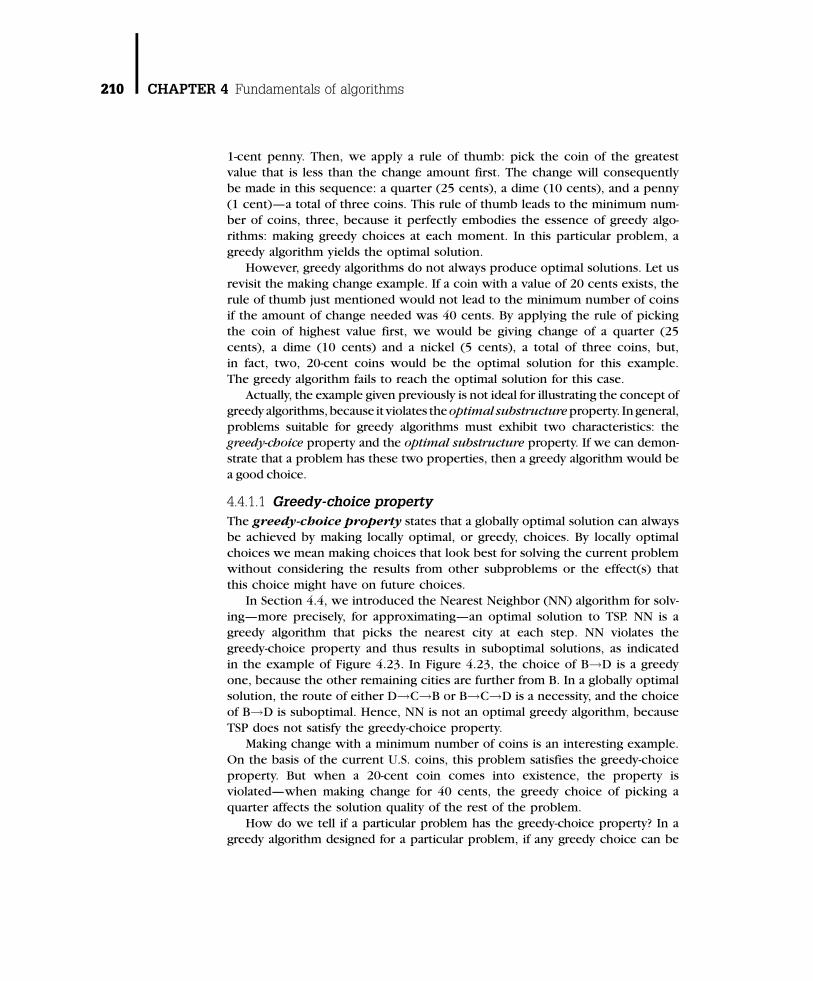
1-cent penny. Then, we apply a rule of thumb: pick the coin of the greatest

value that is less than the change amount first. The change will consequentlybe made in this sequence: a quarter (25 cents), a dime (10 cents), and a penny

(1 cent)—a total of three coins. This rule of thumb leads to the minimum num-

ber of coins, three, because it perfectly embodies the essence of greedy algo-

rithms: making greedy choices at each moment. In this particular problem, a

greedy algorithm yields the optimal solution.

However, greedy algorithms do not always produce optimal solutions. Let us

revisit the making change example. If a coin with a value of 20 cents exists, the

rule of thumb just mentioned would not lead to the minimum number of coinsif the amount of change needed was 40 cents. By applying the rule of picking

the coin of highest value first, we would be giving change of a quarter (25

cents), a dime (10 cents) and a nickel (5 cents), a total of three coins, but,

in fact, two, 20-cent coins would be the optimal solution for this example.

The greedy algorithm fails to reach the optimal solution for this case.

Actually, the example given previously is not ideal for illustrating the concept of

greedy algorithms, because it violates theoptimal substructureproperty. Ingeneral,

problems suitable for greedy algorithms must exhibit two characteristics: thegreedy-choice property and the optimal substructure property. If we can demon-

strate that a problem has these two properties, then a greedy algorithm would be

a good choice.

4.4.1.1 Greedy-choice property

The greedy-choice property states that a globally optimal solution can alwaysbe achieved by making locally optimal, or greedy, choices. By locally optimal

choices we mean making choices that look best for solving the current problem

without considering the results from other subproblems or the effect(s) that

this choice might have on future choices.

In Section 4.4, we introduced the Nearest Neighbor (NN) algorithm for solv-

ing—more precisely, for approximating—an optimal solution to TSP. NN is a

greedy algorithm that picks the nearest city at each step. NN violates the

greedy-choice property and thus results in suboptimal solutions, as indicatedin the example of Figure 4.23. In Figure 4.23, the choice of B!D is a greedy

one, because the other remaining cities are further from B. In a globally optimal

solution, the route of either D!C!B or B!C!D is a necessity, and the choice

of B!D is suboptimal. Hence, NN is not an optimal greedy algorithm, because

TSP does not satisfy the greedy-choice property.

Making change with a minimum number of coins is an interesting example.

On the basis of the current U.S. coins, this problem satisfies the greedy-choice

property. But when a 20-cent coin comes into existence, the property isviolated—when making change for 40 cents, the greedy choice of picking a

quarter affects the solution quality of the rest of the problem.

How do we tell if a particular problem has the greedy-choice property? In a

greedy algorithm designed for a particular problem, if any greedy choice can be


proven better than all of the other available choices at the moment in terms of

solution quality, we can say that the problem exhibits the greedy-choice property.

4.4.1.2 Optimal substructure

A problem shows optimal substructure if a globally optimal solution to it con-sists of optimal solutions to its subproblems. If a globally optimal solution can

be partitioned into a set of subsolutions, optimal substructure requires that

those subsolutions must be optimal with respect to their corresponding subpro-

blems. Consider the previous example of making change of 36 cents with a min-

imum number of coins. The optimal solution of a quarter, a dime, and a penny

can be divided into two parts: (1) a quarter and a penny and (2) a dime. The first

part is, indeed, optimal in making change of 26 cents, as is the second part for

making change of 10 cents.The NN algorithm for TSP lacks both greedy-choice and optimal substructure

properties. Its global solutions cannot be divided into solutions for its subpro-

blems, let alone optimal solutions.

To determine whether a particular problem has an optimal substructure, two

aspects have to be examined: substructure and optimality. A problem has substruc-

tures if it is divisible into subproblems.Optimality is the property that the combina-

tion of optimal solutions to subproblems is a globally optimal solution.

Greedy algorithms are highly efficient for problems satisfying these twoproperties. On top of that, greedy algorithms are often intuitively simple and

easy to implement. Therefore, greedy algorithms are very popular for solving

optimization problems. Many graph algorithms, mentioned in Section 4.3, are

actually applications of greedy algorithms—such as Prim’s algorithm used for

finding minimum spanning trees. Greedy algorithms often help find a lower

bound of the solution quality for many challenging real-world problems.

4.4.2 Dynamic programming

Dynamic programming (DP) is an algorithmic method of solving optimizationproblems. Programming in this context refers to mathematical programming,

which is a synonym for optimization.

DP solves a problem by combining the solutions to its subproblems. The

famous divide-and-conquer method also solves a problem in a similar manner.

The divide-and-conquer method divides a problem into independent subprob-

lems, whereas in DP, either the subproblems depend on the solution sets of other

subproblems or the subproblems appear repeatedly. DP uses the dependency of

the subproblems and attempts to solve a subproblem only once; it then stores itssolution in a table for future lookups. This strategy spares the time spent on recal-

culating solutions to old subproblems, resulting in an efficient algorithm.

To illustrate the superiority of DP, we showhow to efficiently multiply a chain of

matrices by use of DP. When multiplying a chain of matrices, the order of the multi-

plications dramatically affects the number of scalar multiplications. For example,


consider multiplying three matrices A, B, and C whose dimensions are 30 � 100,

100 � 2, and 2 � 50, respectively. There are two ways to start the multiplication:either A � B or B � C first. The numbers of necessary scalar multiplications are:

ðA � BÞ � C : 30� 100� 2þ 30� 2� 50 ¼ 6000þ 3000 ¼ 9000;A � ðB � CÞ : 100� 2� 50þ 30� 100� 50 ¼ 10; 000þ 150; 000 ¼ 160; 000

(A � B) � C is clearly more computationally efficient.

The matrix-chain multiplication problem can be formulated as follows:given a chain of n matrices, <M1, M2, . . . , Mn>, where Mi is a vi�1 � vi matrix

for i ¼ 1 to n, we want to find an order of multiplication that minimizes the

number of scalar multiplications.

To solve this problem, one option is to exhaustively try all possible multipli-

cation orders and then select the best one. However, the number of possible

multiplication orders grows exponentially with respect to the number of matri-

ces n. There are only two possibilities for three matrices, but it increases to

1,767,263,190 possibilities for 20 matrices. A brute-force search might costmore time finding the best order of multiplications than actually performing

the multiplication.

Here, we define m[i, j] as the minimum number of scalar multiplications

needed to calculate the matrix chain MiMiþ1 . . . Mj, for 1 � i � j � n. The target

problem then becomes finding m[1, n]. Because a matrix chain can be divided

into two smaller matrix chains, each of which can be multiplied into a single

matrix first, the following recurrent relationship holds:

m i; j½ � ¼ mini�k<j

m i; k½ � þm kþ 1; j½ � þ vi�1vkvj� �0 if i ¼ j

if i < j

8>><>>: ð4:5Þ

A simple recursive algorithm on the basis of recurrence (4.5) can provide the

answer to m[1, n]; however, such an algorithm will be extremely inefficientbecause, in the process of computing m[1, n], many entries of m[i, j] are com-

puted multiple times. For example, if we wish to compute m[1, 6], the value

of m[3, 4] will be repeatedly computed in the process of calculating m[1, 4],

m[2, 5], and m[3, 6]. However, we could store the values in a table, which leads

to the dynamic programming algorithm BottomUpMatrixChain shown in

Algorithm 4.16.

Algorithm 4.16 A dynamic programming algorithm for solving the matrix-chain

multiplication problem

BottomUpMatrixChain(Vector v)

1. n = v.size – 1;

2. for (i = 1 to n) m[i, i] = 0;

3. for (p = 2 to n) do // p is the chain length


4. for (i = 1 to n – p + 1) do

5. j = i + p – 1;

6. m[i, j] = 1;

7. for (k = i to j - 1) do

8. temp = m[i, k] + m[k + 1, j] + vi-1vkvj;

9. if (temp < m[i, j]) do

10. m[i, j] = temp;

11. d[I, j] = k;

12. end if

13. end for

14. end for

15. return m and d;

The BottonUpMatrixChain perfectly embodies the property of recur-

rence (4.5). A triangular table m[i, j], where 1 � i � j � n, records the mini-

mum numbers of scalar multiplications for its respective matrix chains,whereas another triangular table d[i, j], where 1 � i < j � n, tracks where

the separations of matrix chains should be. We can see in line 3 that the m table

is filled in the ascending order of the length of the matrix chains, so that in line

8, the items to be added are already in place. Finally, the fully filled m and d

tables are returned as answers in line 15.

BottonUpMatrixChain handles recurrence (4.5) by making use of the

repetitive nature of the subproblems. The three loops in lines 3, 4, and 7 indi-

cate that this algorithm has a time complexity of O(n3). Compared with theexponential time needed to search through all possible multiplication orders,

BottomUpMatrixChain is highly efficient.

BottomUpMatrixChain is a typical example of dynamic programming. It

solves the matrix-chain multiplication problem by systematically combining

solutions to multiplication of smaller matrix chains. In fact, the matrix-chain

multiplication problem contains two key ingredients that make BottomUpMa-

trixChain a successful function: overlapping subproblems and optimal sub-

structure. These two properties are indispensable for any DP algorithm to work.

4.4.2.1 Overlapping subproblems

We say that a problem has overlapping subproblems when it can be decom-posed into subproblems that are not independent of one another. Often several

subproblems share the same smaller subproblems. For example, running a

recursive algorithm often requires solving the same subproblem multiple times.

DP solves each subproblem only once and stores the answer in a table, so that


recurrences of the same subproblems take only constant time to get the answer

(by means of a table lookup).The matrix-chain multiplication problem is an instance of this property.

Repeated multiplications of smaller matrix chains cause a high complexity for

a simple recursive algorithm. In contrast, the DP algorithm BottomUpMa-

trixChain creates the m table for the overlapping subproblems to achieve

high efficiency.

4.4.2.2 Optimal substructure

A problem exhibits an optimal substructure if its globally optimal solution con-

sists of optimal solutions to the subproblems within it. Recall that in Subsection

4.4.1, having an optimal substructure ensures that greedy algorithms yield opti-

mal solutions. It fact, if a problem has an optimal substructure, both greedy algo-

rithms and DP could yield optimal solutions. One key consideration in choosing

the type of algorithm is determining whether the problem has the greedy-choice

property, the overlapping subproblems, or neither. If the problem shows overlap-ping subproblems but not the greedy-choice property, DP is a better way to solve

it. On the other hand, if the problem exhibits the greedy-choice property instead

of overlapping subproblems, then a greedy algorithm fits better. A problem rarely

has both of the properties because they contradict each other. The matrix-chain

multiplication problem has an optimal substructure, reflected in recurrence

(4.4), but it does not have the greedy-choice property. It consists of overlapping

subproblems. Therefore, DP is a suitable approach to address this problem.

4.4.2.3 Memoization

BottomUpMatrixChain, as its name suggests, solves the problem iteratively

by constructing a table in a bottom-up fashion. A top-down approach, on the

other hand, seems infeasible, from this simple recursive algorithm. In fact, theunnecessary recomputations that prevent the recursive algorithm from being

efficient can be avoided by recording all the computed solutions along the

way. This idea of constructing a table in a top-down recursive fashion is called

memoization. The pseudocode of a memoized DP algorithm to solve the

matrix-chain multiplication problem is shown in Algorithm 4.17.

Algorithm 4.17 Solving matrix-chain multiplication problems with memoization

TopDownMatrixChain(Vector v)

1. n = v.size – 1;

2. for ( i = 1 to n)

3. for ( j = i to n) m[i, j ] = 1;

4. return Memoize(v, 1, n);

Memoize(Vector v, Index i, Index j)

1. if (m[i, j] < 1) return m[i, j];


2. if (i = j) m[i, j] = 0;

3. else

4. for (k = i to j - 1) do

5. temp = Memoize(v, i, k) + Memoize(v, k + 1, j) + vi-1vkvj;

6. if(temp < m[i, j]) m[i, j] = temp;

7. end for

8. end if

9. return m[i, j];

The time complexity of the TopDownMatrixChain shown in Algorithm

4.17 is still O(n3), because it maintains the m table. The actual runtime of the

TopDownMatrixChain will be slightly longer than the BottomUpMatrix-

Chain because of the overhead introduced by recursion. In general, memoriza-

tion can outperform a bottom-up approach only if some subproblems need not

be visited. If every subproblem has to be solved at least once, the bottom-up

approach should be slightly better.

4.4.3 Branch-and-Bound

Branch-and-bound is a general technique for improving the searching process

by systematically enumerating all candidate solutions and disposing of obviously

impossible solutions.

Branch-and-bound usually applies to those problems that have finite solu-

tions, in which the solutions can be represented as a sequence of options.

The first part of branch-and-bound, branching, requires several choices to bemade so that the choices branch out into the solution space. In these methods,

the solution space is organized as a treelike structure. Figure 4.25 shows an

instance of TSP and a solution tree, which is constructed by making choices

on the next cities to visit.

Branching out to all possible choices guarantees that no potential solutions

will be left uncovered. But because the target problem is usually NP-complete

or even NP-hard, the solution space is often too vast to traverse. The branch-

and-bound algorithm handles this problem by bounding and pruning. Bound-ing refers to setting a bound on the solution quality (e.g., the route length for

TSP), and pruning means trimming off branches in the solution tree whose solu-

tion quality is estimated to be poor. Bounding and pruning are the essential con-

cepts of the branch-and-bound technique, because they are used to effectively

reduce the search space. We demonstrate in Figure 4.25 how branch-and-bound

works for the TSP problem.

The number under a leaf node of the solution tree represents the length of

the corresponding route. For incomplete branches, an expression in the formof a þ b is shown. In this notation, a is the length of the traversed edges, and


b is a lower bound for the length of the remaining route that has not been

explored. The lower bound is derived by use of a minimum spanning tree that

consists of the unvisited vertices, as well as the root and leaf vertices of the par-

tial route. For example, for the unfinished route A!B!E, a minimum spanning

tree is built for nodes A, C, D, and E, and its value is 12. This lower bound is a

true underestimate for the length of the remaining route. The sum of these twonumbers provides the basis for bounding.

The solution tree is traversed depth-first, with the length of the current

shortest route as the upper bound for future solutions. For example, after

A!B!C!D!E!A is examined, the upper bound is 21, and after the next

route is explored, the bound drops to 15. Every time a partial route is extended

by a vertex, a lower bound for the length of the rest of the route is computed.

If the sum a þ b is over or equal to the current upper bound, the solutions on

that branch guarantees to be worse than the current best solution, and thebranch can be pruned. Most branches are pruned in Figure 4.25.

An exhaustive search will build a search tree with 89 nodes,1 but the solu-

tion tree with branch-and-bound has only 20 nodes. Branch-and-bound acceler-

ates the search process by reducing the solution space en masse. Although

branch-and-bound algorithms generally do not possess proven time complexity,

their efficiency has made them the first choice for many problems, especially for

NP-complete problems.

Branch-and-bound mainly addresses optimization problems, because bound-ing is often based on numerical comparisons. TSP that uses the route length

as the bound is a classical application; however, it can also be applied to some

decision problems. In these cases, the bounding criteria are often restrictions or

1Let n be the number of cities and f (n) be the number of nodes in the exhausted search tree.

Then f(2) ¼ 3, f(3) ¼ 7, and f(n) ¼ (n�1)f(n�1) þ 1.

A

B E

C D

2

91

3

8

3

7

5

4 6

A

B

A

B

B

C

C

C

C

C

D

6+12

D

D

EE

E

A

D

E

E

9+10

7+12 7+8 10+8

12+5

12+3

8+10

21 15

FIGURE 4.25

A TSP and its solution tree after applying branch-and-bound.


additional descriptions of possible solutions. The Davis-Putnam-Logemann-Loveland (DPLL) search scheme for the Boolean Satisfiability problem is atypical and important application for this kind of branch-and-bound algorithm.

4.4.4 Simulated annealing

Simulated annealing (SA) is a general probabilistic algorithm for optimization

problems [Wong 1988]. It uses a process searching for a global optimal solution

in the solution space analogous to the physical process of annealing. In the pro-

cess of annealing, which refines a piece of material by heating and controlledcooling, the molecules of the material at first absorb a huge amount of energy

from heating, which allows them to wander freely. Then, the slow cooling pro-

cess gradually deprives them of their energy, but grants them the opportunity to

reach a crystalline configuration that is more stable than the material’s original

form. The idea to use simulated annealing on optimization problems was first

proposed by S. Kirkpatrick, C. D. Gelatt, and M. P. Vecchi in [Kirkpatrick

1983] for the placement and global routing problems.

Simulated annealing (SA) is analogous to annealing in three ways:

1. The energy in annealing corresponds to the cost function in SA. The

cost function evaluates every solution, and the cost of the best-known

solution generally decreases during the SA process. The goal of an optimi-zation problem is to find a solution with a minimum cost.

2. The movements of molecules correspond to small perturbations in the

current solution, such as switching the order of two consecutive vertices

in a solution to TSP. SA repeatedly perturbs the current solution so that

different regions in the solution space are explored.

3. The temperature corresponds to a control parameter temperature T in

SA. T controls the probability of accepting a new solution that is worse

than the current solution. If T is high, the acceptance probability is alsohigh, and vice versa. T starts at the peak temperature, making the current

solution changes almost randomly at first. T then gradually decreases, so

that more and more suboptimal perturbations are rejected. The algorithm

normally terminates when T reaches a user-specified value.

An SA algorithm typically contains two loops, an outer one and an inner one.

In the outer loop, T dwindles every time, and the outer loop terminates when

T reaches some user-specified value. In the inner loop, the solution is perturbed,

and the cost function of the perturbed solution is evaluated. If the new solution

has a lower cost, it directly replaces the current solution. Otherwise, to accept

or reject the new, higher-cost solution is based on a probability function that is

positively related to T and negatively related to the cost difference between the

current and new solutions. The inner loop continues until a thermal equilib-

rium is reached, which means that T also controls the number of iterations


of the inner loop. After both loops terminate, the best solution visited in the

process is returned as the result.The pseudocode in Algorithm 4.18 outlines the SA algorithm. There are a

few details worth discussion: in line 2 of the function Accept, the number

e�DcT ensures that a higher cost solution has a greater likelihood of acceptance

if T is high or the cost difference (△c) is small. Although there is no strong the-

oretical justification for the need of strictly following this exact formula, this for-

mula has been popular among SA users.

Algorithm 4.18 Simulated annealing algorithm

Accept(temperature T, cost Dc)

1. Choose a random number rand between 0 and 1;

2. return (e-Dc/T > rand);

SimulatedAnnealing()

1. solution sNow, sNext, sBest;

2. temperature T, endingT;

3. Initialize sNow, T and endingT;

4. while (T > endingT) do

5. while (!ThermalEquilibrium(T))do

6. sNext = Perturb(sNow);

7. if (cost(sNext) < cost(sNow))

8. sNow = sNext;

9. if (cost(sNow) < cost(sBest))

10. sBest = sNow;

11. else if (Accept(T, cost(sNext)-cost(sNow)))

12. sNow = sNext;

13. end if

14. end while

15. Decrease(T);

16. end while

17. return sBest;

The combination of the functions ThermalEquilibrium, Decrease,

and the parameter endingT in Algorithm 4.18 characterize an SA algorithm.

In combination, they determine the cooling schedule or the annealing sched-

ule. The cooling schedule can be tuned in many ways, such as making T drop

faster at first and slower afterwards in the function Decrease or allowing more

perturbations when T is small in the function ThermalEquilibrium. Every


adjustment in the cooling schedule affects the solution quality and the time

taken to find a solution. In practice, empirical principles and a trial-and-errorstrategy are commonly used to find a good cooling schedule [Hajek 1988].

SA has many advantages over other optimization algorithms. First, because

there is a non-zero probability of accepting higher cost solutions in the search

process, SA avoids becoming stuck at some local minima, unlike some greedy

approaches. Also, the runtime of SA is controllable through the cooling sched-

ule. One can even abruptly terminate this algorithm by changing the parameter

endingT in line 4 of SimulatedAnnealing. Finally, there is always a best-

known solution available no matter how little time has elapsed in the searchprocess. With SA, the user can always get a solution. In general, a longer run-

time would result in a better-quality solution. This flexibility explains SA’s wide

popularity. SA is considered the top choice for several EDA problems, such as

placement and Binary Decision Diagram (BDD) variable reordering.

4.4.5 Genetic algorithms

Just like simulated annealing, genetic algorithms are another general rando-mized algorithm catering to optimization problems [Goldberg, 1989; Davis

1991]. They also perform a series of computations to search for a global optimal

solution in the solution space. As the name suggests, genetic algorithms use

techniques inspired by operations found in evolutionary biology such as

selection, crossover, and mutation.

Genetic algorithms are different from other global search heuristics in many

ways. First of all, other global search algorithms, such as simulated annealing,

perform a series of perturbations on a single solution to approach a global opti-mum. Genetic algorithms simultaneously operate on a set of feasible solutions

or a population. Moreover, the solutions in a genetic algorithm are always

encoded into strings of mathematical symbols, which facilitate future manipula-

tions on them. Many types of coding symbols can be used, such as bits, inte-

gers, or even permutations. In the simplest versions of genetic algorithms,

fixed-length bit strings are used to represent solutions. A bit string that speci-

fies a feasible solution is called a chromosome. Each bit in a chromosome is

called a gene.Genetic algorithms have many variations [Holland 1992]. Here we will focus

on the simple genetic algorithm (SGA) to get a taste of the mechanics of genetic

algorithms. SGA can be separated into six phases: initialization, evaluation,

selection, crossover, mutation, and replacement. After the initial population is

generated in the initialization phase, the other five actions take place in turns

until termination. Figure 4.26 shows the flow of SGA.

In the evaluation phase, chromosomes in the population are evaluated with

a fitness function, which indicates how good the corresponding solutions are.Their fitness values are the criteria of selection in the next phase. Advanced


genetic algorithms can even handle multi-purposed optimization problems with

plural fitness functions.

The selection phase aims at finding the best parents or a group of solutions

to generate the next population. Many schemes can be implemented to exerciseselection in SGA. The simplest scheme is truncation selection, in which the

s chromosomes with the highest fitness values are chosen, and l/s copies are

duplicated for each of them, in which l is the population size. Notice that the

population size will not change after selection. Another simple selection

scheme, Roulette-Wheel selection, chooses a chromosome with the probability

of the ratio of its fitness value to the sum of all fitness values of the population.

In the crossover phase, children chromosomes are produced by inheriting

genes from pairs of parent chromosomes. As always, there are many methods toimplement the crossover, each with its pros and cons. Uniform crossover states

that every gene of a child chromosome comes from a dad with a probability of

p (usually 0.5) and from a mom with a probability of (1 � p). Conventionally,

two parents give birth to two children so that the population size remains

unchanged.

Mutation means changing a tiny fraction of the genes in the chromosomes.

Although in biology mutations rarely happen, they do prevent genetic algo-

rithms from getting stuck in local minima. After the processes of evaluation,selection, crossover, and mutation are complete, the new population replacesthe old one and the next iteration begins.

Figure 4.27 shows a tiny example of an SGA, with a population size of four

and chromosome length of six. The fitness function simply counts “1” genes.

Truncation selection and uniform crossover with a probability of 0.5 are used

in this example. Notice that the average and highest fitness values increase after

one generation.

In this example, the best solution seems very easy to achieve, so an SGAseems unnecessary; however, in real-life applications of SGA, a population size

can be as large as 100,000 and a chromosome can contains up to 10,000 genes.

The fitness function will be much more complex as well.

Mutation

Replacement

Initialization

Evaluation Selection

Crossover

FIGURE 4.26

The flow of a simple genetic algorithm.


SGA is just a small part of the broad subject of genetic algorithms. Geneticalgorithms remain an active research topic for various applications. In addition

to EDA, they have applications in a variety of fields, including designing shapes

for high-speed trains and human face recognition.

4.5 MATHEMATICAL PROGRAMMINGMathematical programming, or mathematical optimization, is a systematic

approach used for optimizing (minimizing or maximizing) the value of an objec-

tive function with respect to a set of constraints. The problem in general can be

expressed as:

Minimize ðor maximizeÞ f ðxÞ;Subject to X ¼ fXjgiðxÞ � bi; i ¼ 1 . . .mg

where

x ¼ ðx1; . . . ; xnÞ are optimization ðor decisionÞ variables;f : Rn ! R is the objective function; and

gi : Rn ! R and bi 2 R form the constraints for the valid values of x

4.5.1 Categories of mathematical programmingproblems

According to the natures of f and X, mathematical programming problems can

be classified into several different categories:

1. If X ¼ Rn, the problem is unconstrained;

2. If f and all the constraints are linear, the problem is called a linear

programming (LP) problem. The linear constraints can then be repre-

sented in the matrix form:

Ax � b

where A is an m � n matrix corresponding to the coefficients in gi(x).

11 0 0 1 0 11 0 0 1 1 11 0 0 0 111 0 0 1 03

11 0 0 1 0 11 0 1 1 1 11 0 1 1 100 0 0 1 12 5

10 0 1 1 1 10 0 0 1 0 11 0 0 1 001 1 0 0 13 3

2

10 0 1 1 010 0 1 1 010 0 1 1 110 0 1 1 14 4

Selection Crossover Mutation

Average fitness: 3Highest fitness: 4

Average fitness: 3.5Highest fitness: 5

FIGURE 4.27

One-generation simulation of a simple genetic algorithm.

4.5 Mathematical programming 221

3. If the problem is linear, and all the variables are constrained to integers,the problem is called an integer linear programming (ILP) problem.

If only some of the variables are integers, it is called a mixed integer lin-

ear programming (MILP or MIP) problem.

4. If the constraints are linear, but the objective function f contains some

quadratic terms, the problem is called a quadratic programming (QP)

problem.

5. If f or any of gi (x) is not linear, it is called a nonlinear programming

(NLP) problem.6. If all the constraints have the following convexity property:

gi axa þ bxbð Þ � agi xað Þ þ bgi xbð Þwhere a � 0, b � 0, and aþ b ¼ 1, then the problem is called a convex

programming or convex optimization problem.

7. If the set of feasible solutions defined by f and X are discrete, the problem

is called a discrete or combinatorial optimization problem.

Intuitively speaking, different categories of mathematical programming problems

should involve different solving techniques, and, thus, they may have different

computational complexities. In fact, most of the mathematical optimization

problems are generally intractable—algorithms to solve the preceding optimiza-tion problems such as the Newton method, steepest gradient, branch-and-

bound, etc., often require an exponential runtime or an excessive amount of

memory to find the global optimal solutions. As an alternative, people turn to

heuristic techniques such as hill climbing, simulated annealing, genetic algo-

rithms, and tabu search for a reasonably good local optimal solution.

Nevertheless, some categories of mathematical optimization problems, such

as linear programming and convex optimization, can be solved efficiently and

reliably. Therefore, it is feasible to examine whether the original optimizationproblem can be modeled or approximated as one of these problems. Once

the modeling is completed, the rest should be easy—there are numerous share-

ware or commercial tools available to solve these standard problems.

In the following, we will briefly describe the problem definitions and solving

techniques of the linear programming and convex optimization problems.

For more theoretical details, please refer to other textbooks or lecture notes

on this subject.

4.5.2 Linear programming (LP) problem

Many optimization problems can be modeled or approximated by linear forms.

Intuitively, solving LP problems should be simpler than solving the general

mathematical optimization problems, because they only deal with linear con-

straint and objective functions; however, it took people several decades to


develop a polynomial time algorithm for LP problems, and several related theo-

retical problems still remain open [Smale 2000].The simplex algorithm, developed by George Dantzig in 1947, is the first

practical procedure used to solve the LP problem. Given a set of n-variable lin-

ear constraints, the simplex algorithm first finds a basic feasible solution that

satisfies all the constraints. This basic solution is conceptually a vertex (i.e., an

extreme point) of the convex polyhedron expanded by the linear constraints

in Rn hyperspace. The algorithm then moves along the edges of the polyhedron

in the direction toward finding a better value of the objective function. It is

guaranteed that the procedure will eventually terminate at the optimal solution.Although the simplex algorithm can be efficiently used in most practical

applications, its worst-case complexity is still exponential. Whether a polyno-

mial time algorithm for LP problems exists remained unknown until the late

1970s, when Leonid Khachiyan applied the ellipsoid method to this problem

and proved that it can be solved in O(n4w) time. Here n and w are the number

and width of variables, respectively.

Khachiyan’s method had theoretical importance, because it was the first

polynomial-time algorithm that could be applied to LP problems; however, itdid not perform any better than the simplex algorithm for most practical cases.

Many researchers who followed Khachiyan focused on improving the average

case performance, as well as the computational worst-case complexity. The

most noteworthy improvements included Narendra Karmarkar’s interior point

method and many other revised simplex algorithms [Karmarkar 1984].

4.5.3 Integer linear programming (ILP) problem

Many of the linear programming applications are concerned with variables only

in the integral domain. For example, signal values in a digital circuit are under a

modular number system. Therefore, it is very likely that optimization problems

defined with respect to signals in a circuit can be modeled as ILP problems.

On the other hand, problems that need to enumerate the possible cases, or

are related to scheduling of certain events, are also often described as ILP.

The ILP problem is in general much more difficult than is LP. It can be shown

that ILP is actually one of the NP-hard problems. Although the formal proof ofthe computational complexity of the ILP problem is beyond the scope of this

book, we will use the following example to illustrate the procedure and explain

the difficulty in solving the ILP problem.

The ILP problem in Figure 4.28 is to maximize an objective function f, with

respect to four linear constraints {g1, g2, g3, g4}. Because the problem consists of

only two variables, x and y, it can be illustrated on a two-dimensional plane,

where each constraint is a straight line, the four constraints form a closed region

C, and the feasible solutions are the lattice or integral points within this region.The objective function f, represented as a stright line to the right of region C,

moves in parallel with respect to different values of k. Intuitively, to obtain


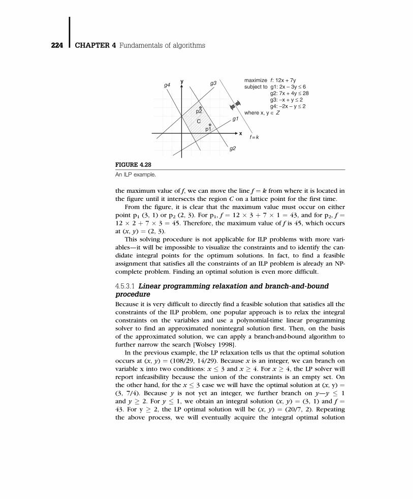
the maximum value of f, we can move the line f ¼ k from where it is located in

the figure until it intersects the region C on a lattice point for the first time.

From the figure, it is clear that the maximum value must occur on either

point p1 (3, 1) or p2 (2, 3). For p1, f ¼ 12 � 3 þ 7 � 1 ¼ 43, and for p2, f ¼12 � 2 þ 7 � 3 ¼ 45. Therefore, the maximum value of f is 45, which occursat (x, y) ¼ (2, 3).

This solving procedure is not applicable for ILP problems with more vari-

ables—it will be impossible to visualize the constraints and to identify the can-

didate integral points for the optimum solutions. In fact, to find a feasible

assignment that satisfies all the constraints of an ILP problem is already an NP-

complete problem. Finding an optimal solution is even more difficult.

4.5.3.1 Linear programming relaxation and branch-and-boundprocedure

Because it is very difficult to directly find a feasible solution that satisfies all the

constraints of the ILP problem, one popular approach is to relax the integralconstraints on the variables and use a polynomial-time linear programming

solver to find an approximated nonintegral solution first. Then, on the basis

of the approximated solution, we can apply a branch-and-bound algorithm to

further narrow the search [Wolsey 1998].

In the previous example, the LP relaxation tells us that the optimal solution

occurs at (x, y) ¼ (108/29, 14/29). Because x is an integer, we can branch on

variable x into two conditions: x � 3 and x � 4. For x � 4, the LP solver will

report infeasibility because the union of the constraints is an empty set. Onthe other hand, for the x � 3 case we will have the optimal solution at (x, y) ¼(3, 7/4). Because y is not yet an integer, we further branch on y—y � 1

and y � 2. For y � 1, we obtain an integral solution (x, y) ¼ (3, 1) and f ¼43. For y � 2, the LP optimal solution will be (x, y) ¼ (20/7, 2). Repeating

the above process, we will eventually acquire the integral optimal solution

maximize f : 12x + 7ysubject to g1: 2x – 3y ≤ 6 g2: 7x + 4y ≤ 28 g3: −x + y ≤ 2 g4: −2x – y ≤ 2 where x, y ∈ Z

x

y

g1

g2

g3g4

f = k

Cp1

p2

FIGURE 4.28

An ILP example.


(x, y) ¼ (2, 3) and f ¼ 45. The decision graph of the branch-and-bound processis shown in Figure 4.29.

4.5.3.2 Cutting plane algorithm

Another useful approach for solving ILP problems is the cutting plane algo-

rithm. This algorithm iteratively adds valid inequalities to the original problem

to narrow the search area enclosed by the constraints while retaining the feasi-

ble points. Figure 4.30 illustrates an example of such valid inequalities.

In Figure 4.30, the cuts c1 and c2 are said to be valid inequalities, because all

the feasible points (i.e., the integral points within the dash region C) are still

valid after adding the new constraints. On the other hand, cut c3 is not a valid

inequality because one feasible point p1 becomes invalid afterward.It is clear to see that the addition of the valid inequality c2 will not help the

search for the optimal solution because it does not narrow the search region.

On the contrary, cut c1 is said to be a strong valid inequality because it makes

the formulation “stronger.” The goal of the cutting plane algorithm is to add

such strong valid inequalities in the hope that the optimal solution will eventu-

ally become an extreme point of the polyhedron so that it can be found by the

polynomial-time LP algorithm.

There are many procedures to generate valid inequalities such as Chvatal-

Gomory [Gomory 1960], 0-1 Knapsack [Wolsey 1999], and lift-and-project

[Balas 1993] cuts. However, sheer use of these valid inequality generation proce-

dures in the cutting plane algorithm will not go too far in solving difficult ILP

x = 108/29y = 14/29

x ≤ 3

x = 3 y = 7/4

y ≥ 2

x = 20/7 y = 2

x ≤ 2

x = 2 y = 7/2

y ≤ 3

x = 2y = 3

f = 45

x = 3y = 1f = 43

infeasible

infeasible

infeasible

FIGURE 4.29

Decision tree of the LP-based branch-and-bound.


problems—it may take an exponential number of steps to approach an integral

extreme point. A better approach would be combining the cutting plane algo-

rithm with the branch-and-bound process. This combined technique is calledthe branch-and-cut algorithm.

4.5.4 Convex optimization problem

As mentioned in Subsection 4.5.1, the constraints in the convex optimization

problem are convex functionswith the following convexity property (Figure 4.31):

gi axa þ bxbð Þ � agi xað Þ þ bgi xbð Þwhere a � 0, b � 0, and aþ b ¼ 1. Conceptually, the convexity property can be

illustrated as follows:

In other words, given two points xa and xb from the set of points defined by a con-

vex function, all thepoints on the line segment between xa and xbwill also belong to

the set (i.e., the dash region),which is called a convex set. Moreover, it can be shown

that for a convex function, a local optimal solution is also a global optimal solution.

In addition, the intersection of multiple convex sets is also convex [Boyd 2004].

p1

x

y

C

c1: x ≤ 4

c2: x+y ≤ 4

c3: 2x+y ≥ 2

FIGURE 4.30

Valid and invalid inequalities.

g(x)

xxaxb

ag(xa) + bg(xb)

g(axa + bxb)

axa + bxb

FIGURE 4.31

The convexity property.


More examples of convex functions can be found in Figure 4.32. The

LP problem, where its constraints form a polyhedron in the n-dimensional

hyperspace, is a special case of the convex optimization problem.

4.5.4.1 Interior-point method

Similar to linear programming, there is, in general, no analytical formula for the

solution of a convex optimization problem. However, there are many effective

methods that can solve the problems in polynomial time within a reasonablysmall number of iterations. The interior-point method is one of the most suc-

cessful approaches.

Although detailed comprehension of the interior-point method requires the

introduction of many mathematical terms and theorems, we can get a high-level

view of the method by comparing it with the simplex method as shown in

Figure 4.33. In the simplex method, we first obtain an initial feasible solution

and then refine it along the edge of the polyhedron until the optimal solution

is reached. In the interior-point method, the initial feasible solution is approxi-mated as an interior point. Then, the method iterates along a path, called a

central path, as the approximation improves toward the optimal solution.

One popular way to bring the interior-point solution to the optimal one is by

the use of a barrier function. The basic idea is to rewrite the original problem

into an equality formula so that Newton’s method can be applied to find the

optimal solution.2

Let’s first define an indicator function I(u) such that I(u) ¼ 0 if u � 0, and

I(u) ¼ 1 otherwise (Figure 4.34). We can then combine the convex objectivefunction min f(x), and the constraints gi(x) � 0 j i ¼ 1 m as:

min f xð Þ þXm1

I gi xð Þð Þ !

Polyhedron formed by linear inequalities hasthe convexity property

(a) (b) (c)

Convex epigraph Non-convex epigraph

FIGURE 4.32

Examples of convex functions.

2To apply the Newton’s method, the formula needs to be an equality and twice differentiable.


This formula describes the same problem as the original convex optimization

problem and after the rewrite, there are no more inequalities. However, this for-

mula is not twice differentiable (i.e., not smooth) near u ¼ 0, so Newton’s

method cannot work. One solution is to use the following logarithmic barrier

function to approximate the indicator function:

BLðu; tÞ ¼ �ð1=tÞlogð�uÞwhere t > 0 is a parameter to control the approximation. As t approaches infin-

ity, the logarithmic barrier function BL(u) gets closer to the indicator function

I(u).

By use of the logarithmic barrier function, the objective function then

becomes:

min f xð Þ þXm1

� 1=tð Þlog �gi xð Þð Þ !

Please note that now the optimization formula is convex and twice differentia-

ble (we assume that both f(x) and gi(x) are twice differentiable here). Therefore,

we can apply Newton’s method iteratively and eventually reach an optimal

initial feasible solutionoptimum

solution

(a) Simplex method

initial feasible solution

optimumsolution

(b) Interior-point method

FIGURE 4.33

Comparison of simplex and interior-point methods.

u

I(u)

−1BL(t) as t ∞

FIGURE 4.34

Indicator I(u) and logarithmic functions BL.


solution. However, please remember that this will be just an approximate solu-tion because of the introduction of the logarithmic barrier function.

The questions then arise: How close is this solution to the solution of the

original problem? What is the effect of t? Intuitively, if t gets larger, the final solu-

tion will be closer to the solution of the original convex optimization problem.

However, with a larger t, it will take a longer time for Newton’s method to con-

verge. On the other hand, the use of a smaller t will lead to a faster solution at

the cost of accuracy.

The pseudocode in Figure 4.35 is an interior-point algorithm that gives asolution balancing runtime and accuracy. We first start with a smaller t so

that Newton’s method converges faster. Once the optimal solution for this

t value is obtained, we then increase t so that the optimal solution gradually

approaches the real optimization of the original problem. This process

terminates when the inverse of the variable t becomes less than the specified

tolerance e.

InteriorMethod (objFunction f, Constraints g)

1. Let (x, t) ¼ min f xð Þ þPm1 � 1=tð Þlog �gi xð Þð Þ� �

2. Given initial t, tolerance e

3. Find an interior feasible point xp s.t. 8i.gi(xp) < 0

4. Starting from xp, apply Newton’s method to find the optimal

solution xopt5. If (1t < e) return optimality as {xopt, (xopt, t)};

6. Let xp ¼ xopt, t ¼ k�t for k > 1, repeat 4

Original constraints: ∏gi(x)

Objectivefunction: f(x)

Optimalsolution

Φ(x, t0)

xpOptimalsolution for t0

Φ(x, t1)for t1 = k⋅t0

xp <= xopt

Optimalsolutionfor t1

FIGURE 4.35

Interior-point algorithm and an illustration of its concept.


4.6 CONCLUDING REMARKSIn this chapter, we present various fundamental algorithms to the EDA research

and development—from the classic graphic theories, the practical heuristic

approaches, and then to the theoretical mathematical programming techniques.

The readers are advised to get acquainted with these algorithms to completely

appreciate the spirit of the research in different areas of the later chapters.In addition, please note that a good EDA algorithm is usually hybrid. In other

words, it should act as a strategy, or say problem-solving tactic that is able to

apply different algorithms in different situations. It should be working efficiently

for the most common cases, taking advantage of the easy ones, and at the same

time, handling the worst-case scenarios gracefully. In summary, do not just take

the algorithms in this chapter as ready solutions; instead, thoroughly understand

the problems first, consider the trade-offs between runtime and memory, and

then treat the algorithms as different utilities, or weapons, for the different chal-lenges in the EDA problem solving process.

4.7 EXERCISES

4.1. (Computational Complexity) Rank the following functions by order

of growth by use of asymptotic notations. One function is neither O( fi)nor O( fi) for any other functions fi. Which is that?

a. 4lg n

b. n � 2nc. n

n � cos n

d. n � lg n

e. (n þ 1)! f. lg999 n g. n � lg n h. n1/lg n

4.2. (Computational Complexity) A Hamiltonian path in a graph is a

simple path that visits every vertex exactly once. The decision problem

HAMILTONIAN PATH for a graph G and vertices u and v asks whether a

Hamiltonian path exists from u to v in G.

a. Prove that HAMILTONIAN PATH is NP.b. Given that HAMILTONIAN PATH is NP-complete, prove that

HAMILTONIAN CYCLE is also NP-complete.

4.3. (Graph Algorithms) Figure 4.36 shows a directed graph of 10 verti-

ces. How many strongly connected components does this graph haveand which are they?

4.4. (Graph Algorithms) Given an undirected, weighted graph G ¼ (V, E )

and two vertices u and v in V. Find an efficient path from u to v such

that the biggest edge weight on the path is minimized.


4.5. (Graph Algorithms) The weighted, undirected graph illustrated in

Figure 4.37 models a combinational circuit. We want to divide these

gates (vertices) into two modules.

4.6. (Heuristic Algorithms) In a dance class, n male students and n female

students should be paired. If we want to minimize the sum of heightdifferences of the n pairs,

a. Design a greedy algorithm to efficiently solve this problem.

b. Prove that the algorithm works because the problem exhibits both

the greedy-choice and optimal substructure properties.

4.7. (Heuristic Algorithms) Solve the matrix-chain multiplication problem

if the dimensions of the matrices are 5 � 10, 10 � 3, 3 � 12, 12 � 5,

5 � 50, and 50 � 6. What are the minimum number of scalar multipli-

cations needed and the order of the multiplications?

4.8. (Heuristic Algorithms) Use the branch-and-bound technique to

solve the TSP problem in Figure 4.38. What is the length of the shortest

route? If only the branching technique is used to form the search tree,what is the number of tree nodes?

4.9. (Linear Programming) Given an n � m rectangular, which is com-

posed of equal-length (length ¼ 1) matches as shown in Figure 4.39.

In this problem, we will try to remove as few as possible matches so

that all the squares (including 1 � 1, 2 � 2, 3 � 3, . . .) in the

A B C D E

JIHGF

FIGURE 4.36

A directed graph to find strongly connected components.

s1

s2

s3

a

b

c

d

e

f

g

t

3

76

12

7

11

8

10

61

8

9

12

7

104

FIGURE 4.37

A model for a combinational circuit in which vertices represent gates and edge weights stand

for the number of connecting wires, where gates s1, s2, and s3 have to be in one module and

t in the other, and meanwhile minimizing the number of wires crossing two modules. What is

the minimal number of crossing wires and where should the cut of two modules be?

4.7 Exercises 231

rectangular are broken. Please model this problem as an integer linear

programming (ILP) problem.

4.10. (Convex Optimization) Prove that a local optimum of a convex

function must be a global optimum.

ACKNOWLEDGMENTSWe thank Dr. Bow-Yaw Wang of Academia Sinica, Taiwan, and Mr. Benjamin Liang of University of

California, Berkeley, for their thorough reviews of the entire chapter, and Professor Tian-Li Yu of

National Taiwan University for providing valuable comments on the “Genetic Algorithm” subsection.

REFERENCESR4.1 Books

[Aho 1983] A. V. Aho, J. E. Hopcroft, and J. D. Ullman, Data Structures and Algorithms, Addison-

Wesley, Reading, MA, January 1983.

[Ahuja 1993] R. K. Ahuja, T. L. Magnanti, and J. B. Orlin, Network Flows: Theory, Algorithms and

Applications, Prentice Hall, Englewood Cliffs, NJ, February 1993.

[Baase 1978] S. Baase, Computer Algorithms: Introduction to Design and Analysis, Addison-

Wesley, Reading, MA, December 1978.

C

DE

F

A B

5

7

453 4 1

3

8

2

6

219 7

FIGURE 4.38

A TSP instance.

n

m

FIGURE 4.39

A square-breaking problem.


[Boyd 2004] S. Boyd and L. Vandenberghe, Convex Optimization, Cambridge University Press,

Cambridge, UK, March 2004.

[Cormen 2001] T. H. Cormen, C. E. Leiserson, R. L. Rivest, and C. Stein, Introduction to Algorithms,

Second Edition, MIT Press, Cambridge, MA, September 2001.

[Davis 1991] L. Davis, Handbook of Genetic Algorithms, Van Nostrand Reinhold, New York, NY,

January 1991.

[Even 1979] S. Even, Graph Algorithms, Computer Science Press, Rockville, MD, June 1979.

[Ford 1962] R. W. Ford and D. R. Fulkerson, Flows in Networks, Princeton University Press, Prince-

ton, NJ, June 1962.

[Garey 1979] M. R. Garey and D. S. Johnson, Computers and Intractability: A Guide to the Theory

of NP-Completeness, W.H. Freeman and Company, San Francisco, CA, January 1979.

[Gibbons 1985] A. Gibbons, Algorithmic Graph Theory, Cambridge University Press, Cambridge,

UK, July 1985.

[Goldberg 1989] D. E. Goldberg, Genetic Algorithms in Search, Optimization and Machine

Learning, Reading, MA, Addison-Wesley, January 1989.

[Holland 1992] J. H. Holland, Adaptation in Natural and Artificial Systems, MIT Press, Cambridge,

CA, April 1992.

[Horowitz 1978] E. Horowitz and S. Sahni, Fundamentals of Computer Algorithms, Computer

Science Press, Rockville, MD, January 1978.

[Knuth 1968] D. E. Knuth, Fundamental Algorithms: The Art of Computer Programming, Volume

1, Reading, MA, Addison-Wesley, February 1968.

[Papadimitriou 1993] C. H. Papadimitriou, Computational Complexity, Reading, MA, Addison-

Wesley, December 1993.

[Papadimitriou 1998] C. H. Papadimitriou and K. Steiglitz, Combinatorial Optimization,

Algorithms and Complexity, Englewood Cliffs, NJ, Prentice Hall, January 1998.

[Reeves 1993] C. R. Reeves, Modern Heuristic Techniques for Combinatorial Problems, McGraw-

Hill, London, UK, February 1993.

[Tarjan 1987] R. E. Tarjan, Data Structures and Network Algorithms, Society for Industrial and

Applied Mathematics, Philadelphia, PA, January 1987.

[Ullman 1984] J. D. Ullman, Computational Aspects of VLSI, Computer Science Press, Rockville,

MD, August 1984.

[Wilf 2002] H. S. Wilf, Algorithms and Complexity, Second Edition, A. K. Peters, Ltd., Wellesley, MA,

December 2002.

[Wong 1988] D. F. Wong, H. W. Leong, and C. L. Liu, Simulated Annealing for VLSI Design, Kluwer

Academic, Boston, MA, March 1988.

[Wolsey 1998] L. A. Wolsey, Integer Programming, Wiley-Interscience, Hoboken, NJ, September

1998.

[Wolsey 1999] L. A. Wolsey and G. L. Nemhauser, Integer and Combinatorial Optimization,

Wiley-Interscience, Hoboken, NJ, November 1999.

R4.2 Computational Complexity

[Knuth 1976] D. E. Knuth, Big Omicron and big Omega and big Theta, in ACM SIGACT News, 8(2),

pp. 18–24, April–June 1976.

R4.3 Graph Algorithms

[Bellman 1958] R. Bellman, On a routing problem, in Quarterly of Applied Mathematics, 16(1),

pp. 87–90, December 1958.

[Dijkstra 1959] E. W. Dijkstra, A note on two problems in connection with graphs, in Numerische

Mathematik, 1, pp. 269–271, June 1959.

References 233

[Edmonds 1972] J. Edmonds and R. M. Karp, Theoretical improvements in the algorithmic efficiency

for network flow problems, in J. of the ACM, 19, pp. 248–264, April 1972.

[Hopcroft 1973] J. E. Hopcroft and R. E. Tarjan, Efficient algorithms for graph manipulation, in Com-

munications of the ACM, 16(6), pp. 372–378, March 1973.

[Moore 1959] E. F. Moore, The shortest path through a maze, in Proc. Int. Symp. on the Theory of

Switching, pp. 285–292, November 1959.

[Prim 1957] R. C. Prim, Shortest connection networks and some generalizations, in Bell System

Technical J., 36, pp. 1389–1401, November 1957.

R4.4 Heuristic Algorithms

[Hajek 1988] B. Hajek, Cooling schedules for optimal annealing, in Mathematics of Operational

Research, 13(2), pp. 311–329, May 1988.

[Kirkpatrick 1983] S. Kirkpatrick, C. D. Gelatt, and M. P. Vecchi, Optimization by simulation anneal-

ing, in Science, 220(4598), pp. 671–690, May 1983.

R4.5 Mathematical Programming

[Balas 1993] S. Balas, S. Ceria, and G. Cornuejols, A lift-and-project cutting plane algorithm for

mixed 0-1 programs, in Mathematical Programming, 58(1-3), pp. 295–324, January 1993.

[Gomory 1960] R. E. Gomory, An algorithm for the mixed integer problem, Research Memoran-

dum, RM-2597, The Rand Corp., 1960.

[Karmarkar 1984] N. Karmarkar, A new polynomial-time algorithm for linear programming, in Proc.

ACM Symposium on Theory of Computing, pp. 302–311, April 1984.

[Smale 2000] S. Smale, Mathematical Problems for the Next Century, in Mathematics: Frontiers and

Perspectives, pp. 271–294, 2000.


fundamentals of algorithms - free160592857366.free.fr/joe/ebooks/sharedata/eda... · in this...

Documents