FUNDAMENTAL PARAMETER METHOD USING SCATTERING X-RAYS IN X-RAY FLUORESCENCE ANALYSIS

Yoshiyuki Kataoka1, Naoki Kawahara1, Shinya Hara1, Yasujiro Yamada1, Takashi Matsuo1, Michael Mantler2

1Rigaku Industrial Corporation,14-8,Takatsuki, Osaka 569-1146, Japan 2Vienna University of Technology, Wiedner Hauptstrasse 8-10, A-1040 Vienna, Austria

ABSTRACT

A new fundamental parameter method which employs measured Compton- and Thomson scattered characteristic tube line intensities for the estimation of non-measuring matrix elements has been developed. The concept of substituting a compound matrix by a single element of average atomic number has been efficiently applied to the analysis of biological samples, polymers, liquids, and powders where the non-measuring elements were unknown. It was found that the divergence of the primary x-ray beam and the resulting range of scattering angles should be accounted for in the calculation of scattering intensities. A computational model using Monte Carlo simulations has been developed which considers the distribution of scattering angles for each geometrical location of the sample, and is used in the quantification routine for actual analysis.

INTRODUCTION

Standardless analysis1) using fundamental parameter methods is a key method for x-ray fluores-cence analysis. However, if unknown non-measurable elements are present in samples such as polymers and biological materials and the elemental composition of the non-measuring elements is not known, accurate analysis was not easily possible. The proposed new method estimates the unknown matrix by measuring Compton- and Thomson scattered characteristic x-ray intensities from the x-ray tube and assumes an element of a corresponding average atomic number to repre-sent an equivalent matrix effect for the analysis in that sample. The idea of average atomic numbers was reported by several authors2,3). However, it was found in our studies that the divergence of the primary x-ray beam and the resulting range of scattering angles should be accounted for in the calculation of scattering intensities. A Monte Carlo simulation model has been developed to con-sider the distribution of scattering angles for each geometrical location within the detectable region of the sample and is used for the standardless quantification routine.

EXPERIMENTAL

The measurements were performed by sequential spectrometers Rigaku ZSX Primus and ZSX Primus-II; both are WDXRF spectrometers and employ Rh target end-window x-ray tubes. The angle of divergence in the primary x-ray beam is about 90 degree. Their Rh-Kα Compton and Thomson scattered lines were measured by using a LiF(220) crystal and scintillation counter. For the other measurements the same standard combinations of crystals and detectors as for regular analyses were employed. 32 standard samples were measured to create the sensitivity calibration. All samples were run without sample backing in order to avoid scattering from the backing mate-rials. A polyester film was used to cover the sample when required and pressed pellets were measured for powder samples. The area density of sample was obtained by measuring sample

255Copyright ©JCPDS-International Centre for Diffraction Data 2006 ISSN 1097-0002

Advances in X-ray Analysis, Volume 49

This document was presented at the Denver X-ray Conference (DXC) on Applications of X-ray Analysis. Sponsored by the International Centre for Diffraction Data (ICDD). This document is provided by ICDD in cooperation with the authors and presenters of the DXC for the express purpose of educating the scientific community. All copyrights for the document are retained by ICDD. Usage is restricted for the purposes of education and scientific research. DXC Website – www.dxcicdd.com

ICDD Website - www.icdd.com

Advances in X-ray Analysis, Volume 49

diameter and sample weight and the thickness was measured by using a vernier calipers in mm. The fundamental parameter method developed in this study is integrated in the standardless analysis software SQX for the ZSX Primus series spectrometers.

CALCULATION OF SCATTERING INTENSITIES

The theoretical model of generating scattering x-rays is illustrated in Fig. 1. It should be noted that any inaccuracy in calculating the theoretical intensities of scattering lines directly affects the analytical results of all elements.

There are two important assumptions in the conventional fundamental parameter method for the calculation of fluorescent x-rays: (1) all in-cident x-rays are irradiated under the same in-cident angle, and (2) all x-rays generated in the sample and emitted at a given observation angle are in principle detectable. However, this as-sumption is not necessarily valid, particularly in view of the angular dependence of the scattering process and the short wavelength (and resulting high penetration power) of the scattering x-rays: As illustrated in Fig. 1, the primary x-ray beams from the x-ray tube are divergent so that the scattering angle varies with the geometrical location of the scattering event; the sample volume which is irradiated by the x-ray tube and also visible to the detector is confined by the divergence of the primary radiation on the tube side as well as by the opening angle of the collimator on the detection side. Considering the short wavelength of Rh-Kα photons and a matrix of light elements, those x-rays can penetrate too deeply into the sample as to be detectable after a scattering process. This geometrical confinement of the detectable region proves important in thick samples of a light matrix including many liquids. This effect is called wedge effect and the combination of the two discussed effects the geometry effect.

In order to estimate the influence of the primary beam divergence, theoretical intensities were calculated for two incident angles, 50° and 60°, and a fixed observation angle, for a range of ele-ments from hydrogen to aluminum. Fig. 2 shows the intensity ratios I60/I50 for Compton and Thomson scattering. While the Compton intensity ratios are close to 1 for all elements, they vary

Figure 2. Influence of incident angle to scattering intensity (Intensity ratios of incident angle: 60 deg to 50 deg)

0.0

0.2

0.4

0.6

0.8

1.0

1.2

1 3 5 7 9 11 13Atomic number

Inte

nist

y ra

tio Rh-Kα Compton

Rh-Kα Thomson

Detector X-ray tube

Sample

Figure 1. Generation of scattering x-rays

X-ray tube

Incident x-raysDivergent

Geometry effect

Sample Detected region

Confined

Detecting system

256Copyright ©JCPDS-International Centre for Diffraction Data 2006 ISSN 1097-0002

Advances in X-ray Analysis, Volume 49

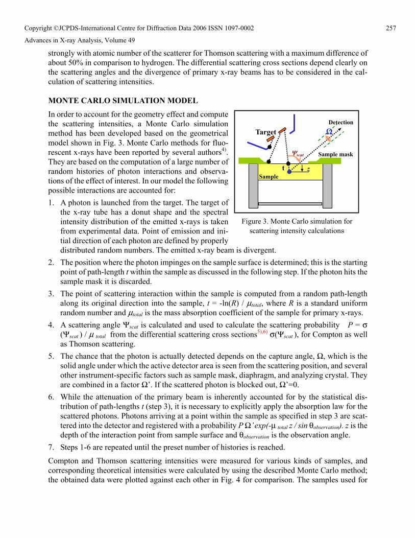
Figure 3. Monte Carlo simulation for scattering intensity calculations

Detection

Ψscat

Ω

Sample mask

Target

Sample t z

strongly with atomic number of the scatterer for Thomson scattering with a maximum difference of about 50% in comparison to hydrogen. The differential scattering cross sections depend clearly on the scattering angles and the divergence of primary x-ray beams has to be considered in the cal-culation of scattering intensities. MONTE CARLO SIMULATION MODEL

In order to account for the geometry effect and compute the scattering intensities, a Monte Carlo simulation method has been developed based on the geometrical model shown in Fig. 3. Monte Carlo methods for fluo-rescent x-rays have been reported by several authors4). They are based on the computation of a large number of random histories of photon interactions and observa-tions of the effect of interest. In our model the following possible interactions are accounted for: 1. A photon is launched from the target. The target of

the x-ray tube has a donut shape and the spectral intensity distribution of the emitted x-rays is taken from experimental data. Point of emission and ini-tial direction of each photon are defined by properly distributed random numbers. The emitted x-ray beam is divergent.

2. The position where the photon impinges on the sample surface is determined; this is the starting point of path-length t within the sample as discussed in the following step. If the photon hits the sample mask it is discarded.

3. The point of scattering interaction within the sample is computed from a random path-length along its original direction into the sample, t = -ln(R) / μtotal, where R is a standard uniform random number and μtotal is the mass absorption coefficient of the sample for primary x-rays.

4. A scattering angle Ψscat is calculated and used to calculate the scattering probability P = σ (Ψscat ) / μ total from the differential scattering cross sections5),6) σ(Ψscat ), for Compton as well as Thomson scattering.

5. The chance that the photon is actually detected depends on the capture angle, Ω, which is the solid angle under which the active detector area is seen from the scattering position, and several other instrument-specific factors such as sample mask, diaphragm, and analyzing crystal. They are combined in a factor Ω’. If the scattered photon is blocked out, Ω’=0.

6. While the attenuation of the primary beam is inherently accounted for by the statistical dis-tribution of path-lengths t (step 3), it is necessary to explicitly apply the absorption law for the scattered photons. Photons arriving at a point within the sample as specified in step 3 are scat-tered into the detector and registered with a probability P Ω’ exp(-μ total z / sin θobservation). z is the depth of the interaction point from sample surface and θobservation is the observation angle.

7. Steps 1-6 are repeated until the preset number of histories is reached.

Compton and Thomson scattering intensities were measured for various kinds of samples, and corresponding theoretical intensities were calculated by using the described Monte Carlo method; the obtained data were plotted against each other in Fig. 4 for comparison. The samples used for

257Copyright ©JCPDS-International Centre for Diffraction Data 2006 ISSN 1097-0002

Advances in X-ray Analysis, Volume 49

Compton scattering in Fig. 4a were powders, polymers, biological samples and liquids, and show good linear relationship without regard to the sample type. The samples measured for Thomson scattering in Fig. 4b were polymers and liquids. The correlation for powder samples is slightly different from that for polymers and liquids. However, both calibrations gave good fits.

QUANTIFICATION The concept of average atomic numbers attempts to replace the actual matrix (of light, non-measuring elements) in a specimen by a single “virtual” element with the same impact upon the analyte line. In the quantification routine it is calculated as a balance component. For the computation of theoretical intensities of fluorescent and scattering x-rays, the following terms for absorption coefficients and scattering cross sections are used:

Scattering cross sections: Compton ΣσCi(λ,ψ)Wi+σ CZav (λ,ψ)WZav

Thomson ΣσTi(λ,ψ)Wi+σ TZav (λ,ψ)WZav

Mass absorption coefficients: Σμi(λ)Wi+ΣμZav (λ)WZav

σC,i, and σT,i are the cross sections for Compton and Thomson scattering, λ is the wavelength of primary x-rays, and Wi is the concentration of analyte element i. Index Zav indicates the “average atomic number” of the virtual balance element. The scattering cross sections and absorption coef-ficients for the virtual atomic number Zav are calculated by interpolation of the scattering cross sections (and absorption coefficients, respectively) over the atomic numbers of actual elements.

The relationship between scattering intensities and atomic numbers of samples was studied in order to allow a suitable choice between Compton and Thomson scattering lines for the determination of the average atomic number. Fig. 5 shows the relationship between Compton and Thomson scat-tering lines as a function of atomic number, for various sample thicknesses.

In the case of Compton scattering (Fig 5a) the intensities drop steeply for thick samples and atomic number greater than 2. This is caused mainly by absorption within the sample. On the other hand, the intensity variations are small for very thin samples: There the scattering intensities are mainly proportional to the Compton scattering cross sections which vary slowly above hydrogen. Con-sequently, Compton scattering can be used for the determination of atomic numbers for thick samples but is not suitable for thin samples.

Figure 4. Sensitivity calibrations for Compton and Thomson scattering lines

0

5

10

15

20

25

0 200 400 600 800Theoretical Intensity

Mea

sure

d In

tens

ity Compton

(a.u

.)

02468

1012

0 50 100 150Theoretical Intensity

Mea

sure

d In

tens

ity

Thomson

(a.u

.)

(b) (a)

258Copyright ©JCPDS-International Centre for Diffraction Data 2006 ISSN 1097-0002

Advances in X-ray Analysis, Volume 49

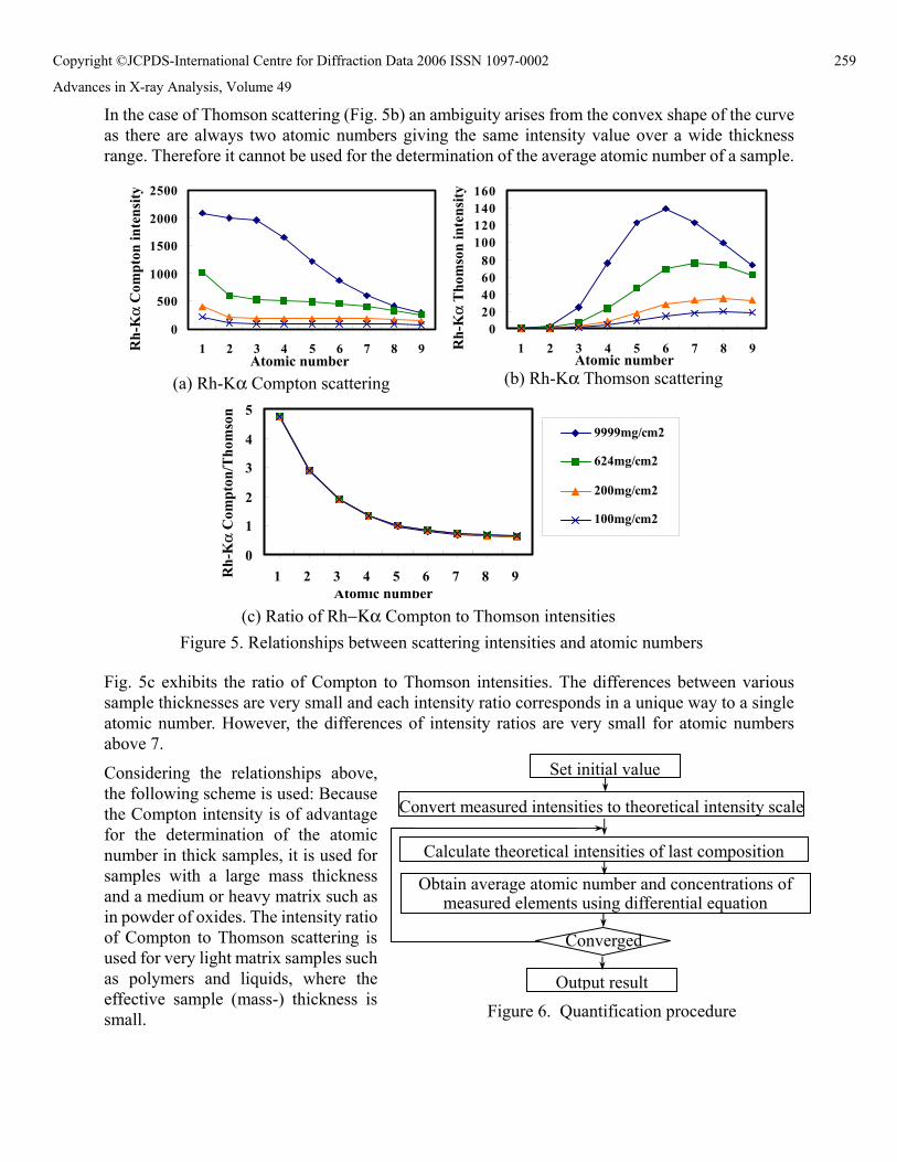
In the case of Thomson scattering (Fig. 5b) an ambiguity arises from the convex shape of the curve as there are always two atomic numbers giving the same intensity value over a wide thickness range. Therefore it cannot be used for the determination of the average atomic number of a sample.

Fig. 5c exhibits the ratio of Compton to Thomson intensities. The differences between various sample thicknesses are very small and each intensity ratio corresponds in a unique way to a single atomic number. However, the differences of intensity ratios are very small for atomic numbers above 7.

Considering the relationships above, the following scheme is used: Because the Compton intensity is of advantage for the determination of the atomic number in thick samples, it is used for samples with a large mass thickness and a medium or heavy matrix such as in powder of oxides. The intensity ratio of Compton to Thomson scattering is used for very light matrix samples such as polymers and liquids, where the effective sample (mass-) thickness is small.

Set initial value

Convert measured intensities to theoretical intensity scale

Calculate theoretical intensities of last composition

Converged

Obtain average atomic number and concentrations of measured elements using differential equation

Output result Figure 6. Quantification procedure

(a) Rh-Kα Compton scattering

(c) Ratio of Rh−Κα Compton to Thomson intensitiesAtomic number

0

1

2

3

4

5

1 2 3 4 5 6 7 8 9

9999mg/cm2

624mg/cm2

200mg/cm2

100mg/cm2

0

500

1000

1500

2000

2500

1 2 3 4 5 6 7 8 90

20406080

100120140160

1 2 3 4 5 6 7 8 9Rh-

Kα

Com

pton

inte

nsity

Rh-

Kα

Tho

mso

n in

tens

ity

Figure 5. Relationships between scattering intensities and atomic numbers

(b) Rh-Kα Thomson scattering Atomic number Atomic number

Rh-

Kα

Com

pton

/Tho

mso

n

259Copyright ©JCPDS-International Centre for Diffraction Data 2006 ISSN 1097-0002

Advances in X-ray Analysis, Volume 49

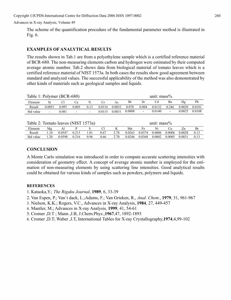
The scheme of the quantification procedure of the fundamental parameter method is illustrated in Fig. 6.

EXAMPLES OF ANALYTICAL RESULTS

The results shown in Tab.1 are from a polyethylene sample which is a certified reference material of BCR-680. The non-measuring elements carbon and hydrogen were estimated by their computed average atomic number. Tab.2 shows data from biological material of tomato leaves which is a certified reference material of NIST 1573a. In both cases the results show good agreement between standard and analyzed values. The successful applicability of the method was also demonstrated by other kinds of materials such as geological samples and liquids. Table 1: Polymer (BCR-680) unit: mass% Element Si Cl Ca Ti Cr As Br Sr Cd Ba Hg Pb Result 0.0051 0.095 0.005 0.13 0.0116 0.0032 0.078 0.004 0.0132 0.246 0.0020 0.0101

Std value - 0.081 - - 0.0115 0.0031 0.0808 - 0.0140 - 0.0025 0.0108

Table 2: Tomato leaves (NIST 1573a) unit: mass% Element Mg Al P S Cl K Mn Fe Ni Cu Zn Br Result 1.10 0.0547 0.213 1.01 0.67 2.78 0.0263 0.0374 0.0006 0.0006 0.0028 0.13

Std value 1.20 0.0598 0.216 0.96 0.66 2.70 0.0246 0.0368 0.0002 0.0005 0.0031 0.13

CONCLUSION

A Monte Carlo simulation was introduced in order to compute accurate scattering intensities with consideration of geometry effect. A concept of average atomic number is employed for the esti-mation of non-measuring elements by using scattering line intensities. Good analytical results could be obtained for various kinds of samples such as powders, polymers and liquids.

REFERENCES 1. Kataoka,Y.; The Rigaku Journal, 1989, 6, 33-39 2. Van Espen, P.; Van`t dack, L.;Adams, F.; Van Grieken, R., Anal. Chem., 1979, 51, 961-967 3. Nielson, K.K.; Rogers, V.C., Advances in X-ray Analysis, 1984, 27, 449-457 4. Mantler, M.; Advances in X-ray Analysis, 1999, 41, 54-61 5. Cromer ,D.T ; Mann ,J.B, J.Chem.Phys.,1967,47, 1892-1893 6. Cromer ,D.T; Waber ,J.T, International Tables for X-ray Crystallography,1974,4,99-102

260Copyright ©JCPDS-International Centre for Diffraction Data 2006 ISSN 1097-0002

Advances in X-ray Analysis, Volume 49