fundamental lower bound for node buffer size in intermittently
TRANSCRIPT

1
Fundamental Lower Bound for Node Buffer Sizein Intermittently Connected Wireless Networks
Yuanzhong Xu and Xinbing WangDept. of Electronic Engineering
Shanghai Jiao Tong University, ChinaEmail: {ukoxyz,xwang8}@sjtu.edu.cn
F
Abstract—We study the fundamental lower bound for node buffer size inintermittently connected wireless networks. The intermittent connectivityis caused by the possibility of node inactivity due to some external con-straints. We find even with infinite channel capacity and node processingspeed, buffer occupation in each node does not approach zero in a staticrandom network where each node keeps a constant message generationrate. Given the condition that each node has the same probability p ofbeing inactive during each time slot, there exists a critical value pc(λ) forthis probability from a percolation-based perspective. When p < pc(λ),the network is in the supercritical case, and there is an achievable lowerbound for the occupied buffer size of each node, which is asymptoticallyindependent of the size of the network. If p > pc(λ), the network is inthe subcritical case, and there is a tight lower bound Θ(
√n) for buffer
occupation, where n is the number of nodes in the network.
1 INTRODUCTION
Scaling properties of capacity, connectivity and delay oflarge-scale wireless networks has received considerableattention in the past several years, since the seminal workon capacity of wireless networks by Gupta and Kumar[1]. Traditionally study on these topics focuses on theassumption of maintaining always full connectivity. How-ever, there is the case where only intermittent connectivitybetween source and destination is guaranteed, thus acomplete path from the source to the destination does notexist all the time. This type of networks are sometimes re-ferred to as Delay/Disruption Tolerant Networks (DTNs)[2]. Properties including capacity, delay and storage ofDTNs, routing schemes and other related network designstrategies have been studied in [3], [4], [5], [6], [7].
We consider wireless networks where intermittent con-nectivity is caused by the possibility of node inactivity orlink inactivity due to some practical constraints, and suchconstraints may vary in different types of networks. In[8], O. Dousse et al. studied the latency of wireless sensornetworks with uncoordinated power saving mechanisms,where constraint on the network is limited node energyand nodes switch between active (on) mode and inactive(off) mode. In [9], W. Ren and Q. Zhao considered acognitive radio network where secondary users should
keep inactive until the availability of wireless channel,and constraint for the secondary networks is the existenceof primary users. In [10], Z. Kong and E. M. Yeh studieda mobile wireless network where the link between twonodes might break (turn inactive) when distance betweenthem is out of the transmission range. One commonfeature of the above three papers is that they are allbased on the theory of percolation (see [13], [14], [15]).These constraints above are external in some sense, whichimplies that inactivity and waiting caused by them cannotbe eliminated via improving processing speed of eachnode or physical conditions of wireless channels. In inter-mittently connected networks, adequate buffer is requiredfor each node to temporarily store the packets not readyto be sent out. With external constraints, the minimumbuffer size requirements for each node do not approachzero as the network capacity and node processing speedapproach infinity. Hence, there exists a lower bound onnode buffer size.
As we know, in an always full-connected wirelessnetwork, buffer is also required for queuing, and queuingdelay is the waiting time between the point of entryof a packet in the transmit queue to the actual pointof transmission. Throughput capacity of mobile wirelessnetworks with limited node buffer has been investigatedby J. D. Herdtner and E. Chong in [11]. In [12], S. Bodaset al. have studied scheduling methods in multi-channelwireless networks in the small-buffer regime. A fun-damental difference of always full-connected networksfrom intermittently connected networks is that if theactual workload of the network keeps constant, queuingdelay and minimum required buffer size decrease as thecapacity and node processing speed increase. Further, asthe capacity and node processing speed of the network goto infinity, the minimum required buffer size and queuingdelay both go to zero.
In this paper we focus on node buffer occupation instatic random wireless networks with intermittent con-
2
nectivity where node inactivity is possible1. To investigatethe fundamental requirements on node buffer size posedby the possibility of node inactivity, we assume thecapacity and node processing speed can be regarded asinfinity, compared with the actual utilization of the net-work capacity. Such assumption makes sense in networkswhere message generation rate is slow and capacity andprocessing speed are adequate. Even if the network ca-pacity and processing speed are limited, results in thispaper present a lower bound on node buffer occupation.As in [8], [9] and [10], we take advantage of percolationtheory to study this problem. To simplify the analysis, weassume each node has the same probability p of beinginactive, and states of nodes (active or inactive) changeover time. We find a critical value for p, pc(λ), where λis the constant node density. If p < pc(λ), the networkis in the supercritical case, where there exists a uniqueinfinite connected cluster of active nodes at any time a.s.when the network size goes to infinity. In contrast, ifp > pc(λ), the network is in the subcritical case, where nosuch infinite cluster exists a.s. when the network size goesto infinity. Minimum buffer occupation is quite differentin the two cases. In the supercritical case, there is anachievable lower bound on occupied buffer size whichis asymptotically independent of the size of the network;while in the subcritical case, buffer occupation increasesas size of the network grows, and there is a tight lowerbound Θ(
√n) for the achievable minimum node buffer
size, where n is the number of nodes.Node buffer requirement is a crucial consideration in
large scale networks where resource of a single node islimited, and a typical type of such network is wirelesssensor networks (WSNs). In [20] and [21], Y. Liu et al. havestudied diagnosis for failures (inactivity) and scalabilityin large WSNs. Since converge-cast is common in WSNs,we will extend the results to converge-cast in our futurework, which can be applied to such WSNs. Further studycan be extended to multicast [18] and mobile networks[19].
This paper is organized as follows. In Section 2, wepresent the network model and some basic assumptions.In Section 3 and 4, we analyze the node buffer occupationin the supercritical case and subcritical case, respectively.In Section 5, we discuss the effects of state-changing fre-quency on buffer occupation, and the results for networkswith finite capacity. Finally, we conclude this paper inSection 7.
2 NETWORK MODEL AND ASSUMPTIONS
2.1 Node Locations and Direct Links
We consider a Poisson point process on R2 with constantpoint density λ. Locations of nodes in the network are
1. For networks with link inactivity, we can get similar results as innetworks with node inactivity, but the analysis is more complicated.
the points within the square region B =[−L
2 ,L2
]2. Let n
denote the number of nodes in the network. According tothe property of Poisson point process, n
λL2 → 1 as L → ∞.Each node covers a disk shaped area with radius r.
To simplify the analysis, r is the same for all nodes. LetXi(1 ≤ i ≤ n) denote the random position of node vi.Two nodes vi and vj are directly connected via a directlink if and only if ||Xvi −Xvj || ≤ 2r, where ||Xvi −Xvj ||is the Euclidean distance between vi and vj . Without lossof generality, we assume 2r = 1.
The set of all nodes in the network is denoted byN (λ, L). When L → ∞, B → R2, the corresponding set ofnodes is defined as N∞(λ) = limL→∞ N (λ,L).
According to continuum percolation theory, there is acritical value for λ, λc, and there exists a unique infiniteconnected cluster in N∞(λ) (giant cluster, denoted byC(N∞(λ))) if and only if λ > λc. To assure the majorityof the network is connected, we make the followingassumption.
Assumption 1 (On Node Density): Node density in thenetwork is large enough to guarantee percolation, i.e.λ > λc.
In this paper, we mainly analyze communications ofnodes within the giant cluster. We denote the nodesbelonging to the giant cluster by the term connected nodes.
For a finite network, we define the giant cluster as thelargest connected cluster in the network. The number ofconnected nodes nc approaches to a constant proportionof n, i.e., nc
n → cλ as n → ∞, where cλ is determined byλ.
2.2 External Constraints and Node Inactivity
In this paper, instead of restricting our study on a specifictype of external constraints, we consider the generaleffects of external constraints on the network: they makeeach nodes switching between active state and inactivestate. During active state, a node can transmit or re-ceive messages, while during inactive state it can neithertransmit nor receive messages. Transmission between twonodes is possible only if both the transmitter and thereceiver are active.
We assume the external constraints in the network arein a synchronized time-slotted manner with a slot lengthTEC , which implies that the state of each node changesonly at the beginning of a time slot. Further, the effectsof external constraints satisfy the following assumptions:
1) States of each active nodes vary from one time slotto another, and are i.i.d. over different time slots.
2) The probability of being inactive is a constant p forall nodes in the network.
3) States of different nodes are i.i.d.The network with external constraints is denoted by
CN (λ,L, p) (or CN∞(λ, p) if L = ∞). Because of thepossibility of node inactivity, we cannot guarantee a
3
complete path connecting a pair of nodes all the time.Hence, the network is intermittently connected.
2.3 Traffic Pattern and BufferingWe only consider the traffic of nodes within C(N (λ, L)),i.e., the connected nodes.
Traffic Pattern of Connected Nodes: For each connectednode in the network, as a source, it randomly choosesa permanent destination among other connected nodes(uniformly), and this source-destination relationship doesnot change over time. Each connected node generatesmessages to its corresponding destination node in a mul-tihop fashion at a constant rate, rg , which does not varyover different nodes.
Buffering: In each hop, if the transmitter or the receiveris inactive, the message should be kept in the buffer ofthe transmitter until both nodes are active. As we definebefore, if a node (as a source) or its first intermediatenode toward destination is inactive, it cannot send anymessage. Yet we can still assume the source node “sends”messages at rate rg but temporarily stored in the bufferof itself.
We define the per-node throughput capacity as the maxi-mum bits per second each connected node can send toits chosen destination node. Now we give a basic as-sumption on channel capacity and per-node throughputcapacity in this paper.
Assumption 2 (On Capacity and Processing Speed): First,the channel capacity for every directly connected nodesis large enough to be viewed as infinity, compared tothe actual transmission rate of each node. As a result,per-node throughput capacity can also be viewed asinfinity compared to rg . Second, node processing speedis also infinitely large, compared to the state-switchingfrequency 1
TEC.
As Assumption 2 states, the capacity of the networkand processing speed is infinity, which implies that oncea node and its next hop turn active, they can transmitand receive message without delay2. If all nodes in onepath are active, the message can be transmitted from oneend to the other without delay. This helps us focus on thelimits posed by intermittent connectivity on node buffersize in the network, and other factors are consideredideal.
Maximum Buffer Occupation in Each Time Slot: Sincethe capacity is infinity, buffered messages in each nodeare transmitted only at the beginning of each time slotwithin a very small time interval. On the other hand,the message generation rate rg is finite and constant,and the buffer occupation of one node will not decrease
2. The propagation delay is omitted in the network. Since the channelcapacity and processing speed is infinity, the queuing delay in each nodeis zero.
but only possibly grow during the time interval exceptthe beginning. Therefore, in each time slot, the size ofoccupied buffer in each node is maximum at the end ofthe time slot. For a connected node w, we use S
(L)w (t) (or
S(∞)w (t)) to denote the occupied buffer size of w at the
end of time slot t in CN (λ,L, p) (or CN∞(λ, p)).Message Slot: We assume the transmission path of each
message does not change if the states of all the nodes inthe network do not change. Therefore, it is obvious thatthe messages generated by one node during one time slotmust exist at the same node at the end of a time slot.We call the messages generated by u during time slot t
whose destination is v a message slot, denoted by m(t)u→v.
If only the source or destination is specified, the notationis simplified as m
(t)u→ or m
(t)→v. If the generating time slot
is not specified, the notations can be further simplifiedas mu→v, mu→ and m→v . The size of one message slot isrgTEC .
2.4 Percolation of Active NodesAccording to Assumption 1, a giant cluster always existsa.s. as the size of the network goes to infinity. Withexternal constraints, for each time slot, we consider thepercolation phenomenon among active nodes.
Since the states of nodes are i.i.d., the distribution ofactive nodes in CN∞(λ, p) is according to a Poisson PointProcess with constant point density (1 − p)λ. Therefore,there exists a critical value for pc(λ) = 1− λc
λ such that:1) If p < pc(λ), CN∞(λ, p) is in the supercritical
case, where there exists a unique infinite connectedcluster of active nodes a.s. during each time slot.Let C(CN∞(λ, p), t) denote the infinite connectedcluster of active nodes (active giant cluster) duringtime slot t.
2) If p > pc(λ), CN∞(λ, p) is in the subcritical case,where there does not exist a unique connected clus-ter of active nodes a.s. during each time slot.
In the supercritical case, C(CN∞(λ, p), t) ⊆ C(N∞(λ)),i.e. the active giant cluster is part of the giant cluster.
To illustrate this point, we first suppose there is anode v ∈ C(CN∞(λ, p), t) but v /∈ C(N∞(λ)). ThenC(N∞(λ)) ∩ C(CN∞(λ, p), t) = ∅, because otherwise vcan connect to C(N∞(λ)) through the nodes belongingto both sets. Therefore, there exist two disjoint infiniteconnected clusters in N∞(λ), which contradicts the factthat C(N∞(λ)) is unique.
Let θ(λ, p|active) denote the probability that an activenode belongs to the active giant cluster in an arbitrarytime slot, then we have
θ(λ, p|active){
> 0, p < pc(λ)= 0, p > pc(λ)
.
The definition of supercritical and subcritical casesabove is in terms of infinite-sized network. However,

4
when the network size is finite, we can also use thevalue of p to determine which case it belongs to. Bufferoccupations in the two cases behave quite differentlywhen we let the network size approach infinity. Ourwork will focus on the order of the buffer occupation as afunction of the network size in the two cases respectively.
3 LOWER BOUND FOR BUFFER SIZE IN THESUPERCRITICAL CASE
In this section, we study the achievable lower boundfor buffer size of connected nodes in CN (λ,L, p) whenp < pc(λ). The main result is that the expected value ofminimum buffer occupation of each connected node isasymptotically independent of the size of the network, asstated in Theorem 1.
Theorem 1: For a uniformly randomly selected con-nected node w in CN∞(λ, p) with p < pc(λ), at the endof an time slot t,
E(S(∞)w (t)
)≥ b1rgTEC . (1)
And it is achievable with some routing scheme that
E(S(∞)w (t)
)≤ c1rgTEC < ∞. (2)
b1 and c1 are positive constants, and rgTEC is the length ofeach message slot. The lower bound b1rgTEC holds for allpossible schemes, while the upper bound c1rgTEC holdsin the optimal case. Therefore, Θ(1) is the fundamentalachievable lower bound for buffer size in the supercriticalcase.
3.1 Proof of Inequality (1)
For the lower bound in Inequality (1), each connectednode should at least buffer the messages generated byitself before it and its neighbors turn active. Since at leastthe source should be active when it sends out a message,the average waiting time before a message is sent out ofits source is larger than TEC
1−p . Applying Little’s Law,
E(S(∞)w (t)
)≥ rgTEC
TEC
TEC(1− p)= b1rgTEC ,
where b1 is determined by p, which does not depend onthe size of the network.
In the following parts of this section, we first present arouting scheme, and then prove that under this scheme,the buffer size requirement specified in Inequality (2) isachieved.
3.2 Optimal Routing SchemeAssumption 3 (On ORS): In Optimal Routing Scheme
(ORS), we assume that each connected node knowswhether it belongs to the active giant.
Assumption 3 is important in the Optimal RoutingScheme which relies on the active giant. Before describingthe ORS, we first introduce the source extending path.
3.2.1 Source Extending Path (SEP)Starting from each connected node, we draw a ray witha permanent random direction, and let Ru denote theray starting from u. Then divide the ray into a string ofsegments of constant length ls, as illustrated in Fig. 1.The nearest connected node to each segment endpointsis a flag node, and we connect every two neighboring flagnodes by the shortest path. After that, if any node in thepath overlaps with more than two other nodes in thepath, remove the redundant nodes, as shown in Fig. 1.The infinite path starting from u is termed as its sourceextending path of u (SEPu). In Optimal Routing Scheme,each message slot is first transmitted along the sourceextending path.
u
Flag Nodes: nearest connected nodes to segment endpoints
Ru
u
Remove the redundant nodes.
Ru
Fig. 1. Source Extending Path.
3.2.2 Optimal Routing SchemeThere are 3 stages of message forwarding in the optimalrouting scheme. Consider the transmission of messageslot mu→v.
I Source u starts sending mu→v along its source ex-tending path SEPu hop by hop, and each node onthe path keeps a copy of mu→v. Before transmissionon each hop begins, the node that newly receivedmu→v in the source extending path must finish send-ing mu→v to its other neighbors that do not belong toSEPu, as shown in Fig. 2. 3 This process stops whenany node that has received the messages belongs tothe active giant, C(CN∞(λ, p), t). At the end of thisstage, the set of nodes that contains a copy of mu→v
(including nodes on SEPu and their neighbors) iscalled the source buffering path of mu→v, SBPmu→v .
3. This is to make sure that there are no nodes that intersect the sourceextending path but do not have the copy of mu→v , which is necessaryin the proof of Lemma 1.

5
node type
has received the message slot?
belongs to SEP?
Y Y
Y Y
N N
N N
Fig. 2. Message transmission in the first stage.
II In this stage, the message is forwarded as near tothe destination as possible. Assume w1 in the sourcebuffering path belongs to the active giant in timeslot t, i.e. w1 ∈ C(CN∞(λ, p), t) ∩ SBPmu→v . Thetransmission starts from w1 but no longer along SEP.Instead, w1 sends the messages generated and beinggenerated by the source to w2 via the shortest pathin C(CN∞(λ, p), t), where
w2 = argminw′∈C(CN∞(λ,p),t)
||Xw′ −Xv||,
i.e., w2 is the nearest node in C(CN∞(λ, p), t) tov. 4 When this transmission is performed, nodes inSBPmu→v release the copies of mu→v.
III In the last stage, we select the shortest path fromw2 to v as the destination buffering path of mu→v,DBPmu→v . mu→v is further transmitted hop by hopalong DBPmu→v . During each hop, if the transmitteror the receiver is inactive, the messages should bebuffered in the transmitter until both are active.
We define the source buffering radius and destina-tion buffering radius of message slot mu→v, denoted byRSBmu→v and RDBmu→v , as
RSBmu→v = maxwi∈SBPmu→v
||Xwi −Xu||,
RDBmu→v = maxwi∈DBPmu→v
||Xwi −Xv||.
With ORS, we can prove that buffer occupation ineach connected node is finite. Since in each time slot theactive giants exists, SBR and DBR cannot be very large.Therefore, each connected node needs only to buffer themessages from near sources or to near destinations. Thatis the intuition of the proof of Inequality (2) with ORS.
3.3 Finite Buffering Radius
With ORS, both the source buffering path and destinationbuffering path are finite, as more precisely demonstratedin the following lemma.
Lemma 1: For a uniformly randomly chosen messageslot mu→v, its corresponding buffering radii RSBmu→v
and RDBmu→v satisfy
P(RSBmu→v ≥ R) ≤ βs(R+ 1)e−αsR, and
P(RDBmu→v ≥ R) ≤ βd(R+ 1)e−αdR,
4. If v ∈ C(CN∞(λ, p), t), then w2 = v.
v
w
Destination Buffering Path
Destination Buffering Radius
u
not received messages
Source Buffering Path
(received messages)
u
vw
Source Buffering Radius
Stage I
Stage II
Stage III
2
w1
containing active giant
2
Inactive node
Active node
Fig. 3. Optimal Routing Scheme.
where αs, αd and βs, βd are constant with αs, αd > 0 andβs, βd < ∞.
Proof: The proof will use the concept of vacant com-ponents. A vacant component means a continuous areathat is not covered by nodes, see [14]. As we onlyconsider active nodes here, a vacant component meansa continuous area that is not covered by active nodes.
We first prove the result for RDB. Consider the distancebetween v and the first node in DBPmu→v , w2. Accordingto ORS, at the time when w2 receives mu→v (the end ofStage II), there is no node belonging to C(CN∞(λ, p), t)within the circle centered at v with radius r = ||Xw2 −Xv|| − 1
2 .5 It implies that a vacant component surroundsthe circular area, including every diameter of it. We onlyconsider the horizonal diameter of this circle, which isadequate to prove the result.
Let Sgv(d) denote the horizonal line segment centeredat v with length d. Utilizing Lemma 6 in Section 6, wehave
5. Here 12
is the radius of the coverage area of node w2.

6
(Only active nodes are shown in this figure.)
w
v
2
Sg (d)v
RDB
Fig. 4. A vacant component surrounding the circularregion.
P(||Xw2 −Xv|| ≥ R)
≤ P(Sgv(2R− 1) is circulated by a vacant component)
≤ βe−α(2R−1) = β′de
−α′dR
where α′d and β′
d are constants with α′d > 0 and β′
d < ∞.
Now we have proved that the distance from w2 to vcannot be very large. However, RDB can be larger thanthe distance from w2 to v (see Fig. 5). We are going tofurther prove the corresponding result for RDB.
Active nodes Inactive nodes
v
w
RDB
Destination Buffering Path
2
||X -X ||w2v
Fig. 5. An example that RDB is larger than the distancefrom w2 to v.
In Fig. 6, the shaded region contains a close circuitof connected nodes (the event that the shaded regioncontains a close circuit is denoted by event Ed, whered is the side length of the square). Lemma 2 in [8] showsthat P(Ed) ≥ 1 − β′
cde−α′
cd where α′c > 0 and β′
c < ∞.If Ed happens, DBPmu→v is within the square, and thusRDBmu→v ≤
√2d.
P(RDBmu→v ≥ R)
≤ P({
||Xv −Xw2|| ≥ R
2
}∪ E R√
2
)≤ P
(||Xv −Xw2 || ≥
R
2
)+ 1− P
(E R√
2
)≤ β′
de−α′
dR/2 +β′c√2Re
− α′c√2R
≤ βd(R+ 1)e−αdR,
d/4
d
v
w
Fig. 6. w2 and v are enclosed in a circuit of connectednodes.
where αd and βd are constants with αd > 0 and βd < ∞.
The proof of RSB can utilize a similar approach as RDB.Recall the transmission of mu→v in Stage I. Since theSBP contains a continuous chain of nodes on the sourceextending path SEPu, and nodes directly overlap withthem, then in Stage I, the active giant cannot intersectwith SBP. In other words, in Stage I, SBP is circulated bya vacant component.
Here in Stage I, ORS requires transmission on eachhop of SEP must guarantee all the transmitter’s directneighbors have receive copies of the messages. This isnecessary for the statement: in Stage I, the active giantdoes not intersect with SBP. As Fig. 7 shows, it is possiblein Stage I that active giant can intersect with SEP (vianodes x and y). If SBP only contains nodes of SEP, then theactive giant can overlap with SBP (part of SEP), thus inthis case the result of vacant component is not applicable.On the other hand, as long as the direct neighbors of
Active node not belonging to SEP
Inactive nodes belonging to SEP
x
y
Fig. 7. Active giant intersects with SEP in Stage I.
nodes in SEP also receive and keep copies of the message,i.e. x and y also belongs to SBP, the statement above isvalid
We assume mu→v is generated in time slot t0, Stage Istops in time slot t− 1, and Stage II starts from time slott. Then for each time slot between t0 and t − 1, there isa vacant component circulating the nodes that receivedmu→v. Specifically, we consider the vacant component in

7
time slot t− 1. As in Corollary 1 in Section 6, we denotethe event that u is circulated by a vacant component withdiameter larger than 2R by EV (d>2R)(u), then
P(RSBmu→v ≥ R) ≤ P(EV (d>2R)(u))
≤ β′(2R+ 1)e−α′2R ≤ βs(R+ 1)e−αsR,
where αs and βs are constants with αs > 0 and βs < ∞.
Lemma 1 indicates that the probability that a nodebelongs to the source (or destination) buffering radius ofa message slot is very small when it is far from the source(or destination).
P(w ∈ SBPmu→v ) ≤ βs(||Xw −Xu||+ 1)e−αs||Xw−Xu||,
P(w ∈ DBPmu→v ) ≤ βd(||Xw −Xv||+ 1)e−αd||Xw−Xv||.
3.4 Finite Hops and LatencyWe have shown that the ranges of SBP and DBP tendto have relatively small values, and so do the numberof hops on SBP and DBP. For SBP, “one hop” meansthe transmission from two neighboring nodes in thesource extending path. Let NSBmu→v and NDBmu→v
respectively denote the number of hops on SBPmu→v andDBPmu→v .
Lemma 2: For a randomly selected mu→v,
P(NSBmu→v ≥ N) ≤ βsh(√N + 1)e−αsh
√N ,
P(NDBmu→v ≥ N) ≤ βdh(√N + 1)e−αdh
√N ,
where αsh, αdh and βsh, βdh are constant with αsh, αdh > 0and βsh, βdh < ∞.
Proof:First we consider NDBmu→v . Since DBP is the shortest
path connecting w2 and v, a node cannot overlap morethan two other nodes of the path. Otherwise, one nodecan be removed to shorten the path. Therefore, such apath with l nodes will cover at least an area with sizeπr2l = lπ
4 . On the other hand, this area should be withinthe circular region centered at v with radius RDBmu→v .
P(NDBmu→v ≥ N) ≤ P(πN
4≤ πRDB2
mu→v)
≤ P(RDBmu→v ≥√N
2) ≤ βd(
√N
2+ 1)e−αd
√N2
≤ βdh(√N + 1)e−αdh
√N .
The proof for RSBmu→v is the same as NDBmu→v , sincethe construction of SEP has also excluded the case thatone node overlaps with three or more other nodes in thepath.
In ORS, transmission latency only happens in Stage Iand III. In Stage III, the single-hop-delay is (note that onenode is active when it receives a message)
E(T d1 ) = TEC
∞∑k=1
p(1− p)2(1− (1− p)2)k−1k =pTEC
(1− p)2.
While in Stage I, the single-hop-delay is relatively largersince in each hop the transmitter must assure the messageis sent to all its direct neighbors, but it still has finiteexpectation E(T s
1 ). Since the buffering hops in each stageis finite a.s., the transmission latency of each message slotis also finite. Consequently, the expected numbers of suchmessage slots mu→ existing in their SBP’s and of suchm→v existing in their DBP’s are both finite, denoted byEs and Ed (u and v are randomly selected).
3.5 Finite Buffer OccupationIn this section we finally present the proof that Inequality(2) holds when Optimal Routing Scheme is applied.
Proof of Inequality (2): In ORS, buffering can happenboth in Stage I (source buffering) and Stage III (destina-tion buffering). We first discuss source buffering. For arandomly selected connected node u, let Ms
u(w, t) denotethe number of such message slots mu→ that are bufferedin w in time slot t. According to Lemma 1,
E(Msu(w, t)) ≤ Esβs(||Xw −Xu||+ 1)e−αs||Xw−Xu||.
Consider the ring centered at w with radius r and width∆r (r >> ∆r), and the expected number of nodes insidethis ring is 2λπr∆r. We first consider how many messageslots from this ring are buffered in w, then let r rangefrom 0 to infinity and thus we can get the expected totalnumber of message slots buffered in w, and thus get theexpected value of the part of buffer occupation of w wherew serves for SBP.
r
w
Δr
Fig. 8. The ring centered at w with radius r and width ∆r.The expected number of nodes it contains is 2λπr∆r.
E(S(∞)w,SBP (t)
)≤ rgTEC
∫ ∞
0
2λEsβs(r + 1)e−αsrπrdr
= csrgTEC .
For destination buffering, we correspondingly have
E(S(∞)w,DBP (t)
)≤ cdrgTEC .
Finally, the buffer occupation of w is the sum of theabove two parts,
E(S(∞)w (t)
)≤ (cs + cd)rgTEC = c1rgTEC ,
where c1 is determined by p and λ, which does notdepend on the size of the network.

8
The lower bound b1rgTEC in Inequality (1) holdsfor all possible schemes, while the upper boundc1rgTEC in Inequality (2) holds with ORS. Therefore,Θ(1) is the fundamental achievable lower bound forbuffer size in the supercritical case with respect to n or L.
4 LOWER BOUND FOR BUFFER SIZE IN THESUBCRITICAL CASE
If p > pc(λ), the network is in the subcritical case. In thiscase, the active giant cluster does not exist during eachtime slot a.s. Therefore, when the size of the network goesto infinity, without utilizing the active giant, transmissionlatency should also go to infinity. Hence, the entire pathfrom the source to the destination should buffer themessages.
In the optimal case, the achievable lower bound fornode buffer size is presented in Theorem 2.
Theorem 2: Buffer occupation of connected nodes in thesubcritical case follows:
1) The average buffer occupation among all connectednodes in CN (λ,L, p), denoted by S
(L)(t), has a
lower bound on Θ(L), or equivalently Θ(√n), and
limL→∞
S(L)
(t)
L≥ b2rgTEC .
2) For a randomly selected connected node w inCN (λ,L, p) with p > pc(λ), at the end of time slot t,it is achievable that
limL→∞
E
(S(L)w (t)
L
)≤ c2rgTEC < ∞.
b2, c2 are finite positive constants irrelevant to L, andrgTEC is the length of each message slot.
Because of the square shape of the network region,nodes in the central part would need larger buffer thannodes near the rim. Fortunately, the edge effects do notchange the order of the required buffer size with respectto L or n; it is achievable that the expected value ofminimum required buffer size of each connected node hasa common upper bound. We will first give a theoreticallower bound on the minimum required buffer size, andthen prove it can be achieved, via presenting a construc-tive upper bound.
4.1 The Lower bound on the Average Buffer Occupa-tionIn this subcritical intermittently connected network, thefollowing lemma on the minimum message existing time(delay) can be proved.
Lemma 3: If (1 − p)λ < λc, the minimum latency ofmessage slot mu→v , Tmu→v , satisfy
lim||Xu−Xv||→∞
Tmu→v
||Xu −Xv||= γ > 0 a.s.
Proof for this lemma is based on the SubadditiveErgodic Theorem [16], and is similar to the proof ofTheorem 1 in [8], where the only difference is that stateswitching in [8] is asynchronous (uncoordinated). Theo-rem 1 in [8] shows that in subcritical case, the minimumdelay from X to Y (T (X,Y )) satisfies
(1− ϵ)η ≤ T (X,Y )
|X − Y |≤ (1 + ϵ)η
for any ϵ > 0 whenever |X − Y | is large enough,where |X − Y | is the distance between X and Y . Hence,lim|X−Y |→∞
T (X,Y )|X−Y | = γ′ > 0, a.s. In the proof of Theorem
1 in [8], state switching only affects the average one-hopdelay, and the condition that the one-hop delay is finite(toff ) is sufficient for the proof. In this paper, though stateswitching is synchronous, since the one-hop delay is alsofinite, the proof method in Theorem 1 in [8] is still validfor Lemma 3 in this paper and the result is the same.
Since each connected node uniformly randomlychooses a destination, the average distance of source-destination pairs is of the order Θ(L), or equivalently,Θ(
√n). Therefore, the average minimum latency for a
message slot is Θ(√n). Since messages are generated con-
tinuously, by Little’s Law, the average number of messageslots generated by one node existing in the network ina given time slot is Θ(
√n). There are Θ(n) connected
nodes, thus the number of all message slots existing ina given time slot is Θ(n
√n). Hence, the average number
of message slots one connected node should buffer isΘ(
√n).
Θ(√n) is a lower bound on the average minimum
required buffer size of each connected node. Take thelength of each message slot, rgTEC , into consideration,we have
limL→∞
S(L)
(t)
L> b2rgTEC .
4.2 A Constructive Upper bound on the MinimumBuffer Occupation for All NodesIn this section, we will present a scheme in which a Θ(
√n)
buffer size requirement can be achieved in the subcriticalcase. To achieve this, we designate a permanent pathfor each source-destination pair where the number ofhops is asymptotically linear to the distance betweenthem. The path is similar to the source extending pathin supercritical case, but has two ends.
For a source node u, and its destination v, we drawa straight line Lv
u connecting them, and divide it intosegments with constant length ls, as shown in Fig.9. The end points are denoted by {EPu→v
i }, i =0, 1, ..., ⌊||Xu −Xv||/ls⌋. At each end point of the seg-ments, we choose the nearest connected node as a flagnode in the path from u to v. The set of flag nodes is de-noted by {NFu→v
i }, i = 0, 1, ..., ⌊||Xu −Xv||/ls⌋. Connect

9
u vEPu v2
Flag Nodes: nearest connected nodes to segment endpoints
Fig. 9. The permanent path from u to v.
every two neighboring flag nodes with the shortest pathbetween them, and thus we get the path from u to v,Pu→v. Denote the segment of the path between NFu→v
i−1
and NFu→vi by PSu→v
i . All the messages generated by uis transmitted along this path.
This scheme assures that the number of hops in Pu→v
is asymptotically linear to the ||Xu −Xv|| (see [8]). Sincethe delay on each hop is finite
(pTEC
(1−p)2
), the average
latency is Θ(√n). We are going to show how many
paths a connected node belongs to, and then give theupper bound on the minimum required buffer size in thesubcritical case.
Lemma 4: A connected node w belongs to at mostΘ(
√n) paths connecting source-destination pairs.Proof: Applying the same technique as in the proof
of Lemma 1, if a square connected circuit that surroundsEPu→v
i−1 and EPu→vi , then PSu→v
i must be within thiscircuit. Then if w belongs to PSu→v
i , it must be inside thesmallest one of such circuits, and there is no such circuitswith smaller size than the distance between w and thesegment. Therefore,
P(w ∈ PSu→vi )
≤ βp(||Xw − EPu→vi ||+ 1)e−αp||Xw−EPu→v
i ||,
where βp and αp are constants with αp > 0 and βp < ∞.Assuming the distance between w and Lv
u is dw,Lvu
, wecan calculate the probability that w belongs to Pu→v.Divide {EPu→v
i } into two subsets (as in Fig. 10): one
dEPXvu
iw2>−
→dEPX
vu
iw2<−
→
u v
d
w
EPu v2 PFu v
w
Fig. 10. Calculate the probability that w belongs to Pu→v.
includes endpoints within distance√2dw,Lv
uto w, the
other includes endpoints outside this distance. For thefirst subset, ||Xw − EPu→v
i || ≤ dw,Lvu
; and for the secondsubset, ||Xw − EPu→v
i || > ||EPu→vi − PFu→v
w ||, wherePFu→v
w is the perpendicular foot from w to Lvu.
P(w ∈ Pu→v)
≤∑i
P(w ∈ PSu→vi )
≤∑
||Xw−EPu→vi ||<
√2dw,Lv
u
P(w ∈ PSu→vi ) +
∑||Xw−EPu→v
i ||>√2dw,Lv
u
P(w ∈ PSu→vi )
≤ β1dw,Lvu(√2dw,Lv
u+ 1)e−α1dw,Lv
u +
β2dw,Lvue−α2dw,Lv
u
≤ β(d2w,Lvu+ 1)e−αdw,Lv
u ,
where β and α are constants with α > 0 and β < ∞. Sincethe edge effects, nodes in the central region needs largerbuffer size, and we assume w is located at the center ofthe network. Suppose ||Xu −Xw|| = R, then there existsa constant c2 that for all possible u, v and w with R > r,
P(r < dw,Lvu< r +∆r|R > r) < c3
∆r
R.
If R < r, P(r < dw,Lvu
< r + ∆r|R < r) = 0. Fig. 11illustrates the case when R > r. Then we calculate theexpected number of lines intersecting the ring centered atw with radius r and width ∆r, denoted by NLw(r,∆r).
E(NLw(r,∆r))
≤∫ L√
2
r
2πRλc3∆r
RdR
≤ c4L∆r.
r
u
w
RΔr
Fig. 11. Calculate the probability that Lvu intersects the
ring centered at w with radius r and width ∆r. The shadedregion is the possible area where v is located.
Let NPw denote the total number of paths connecting

10
source-destination pairs that w belongs to, then we have
E(NPw)
≤∫ L√
2
0
E(NLw(r,dr))β(r2 + 1)e−αr
≤∫ L√
2
0
c4Lβ(r2 + 1)e−αrdr
≤ c5L.
Therefore, w belongs to at most Θ(√n) paths connecting
source-destination pairs.If w ∈ Pu→v, then the expected number of message
slots generated by u that are buffered in w is of aconstant order, after buffering in the network becomesstable. Therefore, the expected number of all messageslots buffered in w is linear to the number of paths itbelongs to. Lemma 4 gives an upper bound on this value,
limL→∞
E
(S(L)w (t)
L
)< c2rgTEC < ∞.
We get this upper bound when w is at the center ofthe network. Taking edge effects into consideration, thisupper bound still applies to all connected nodes. Hence,Theorem 2 is proved.
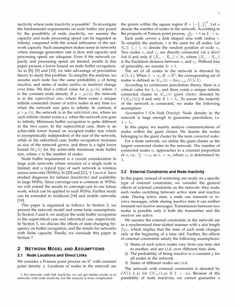
4.3 Variations in Time DomainEach hop of one path has a constant expected buffer occu-pation (only considering the messages generated by thesource of this path). Now we use simulation to investigatethe variations (fluctuations) of buffer occupation overpath. The path consists of 1000 nodes, and the probabilityof being inactive is 0.5. From Fig. 12, we can see that asthe number of hops from source increases, the variation ofbuffer occupation in one node also increases, and bufferoccupation is intensive in a small portion of time but isempty in most of time, as shown in Fig. 12.
This phenomenon can be viewed as an accumulationof messages due to the inactivity. For instance, considerthe i-th and (i + 1)-th nodes. If the (i + 1)-th node staysinactive for several time slots, the messages are likely toaccumulate at the i-th node. Although one node is notvery likely to stay inactive for a long period, on a longpath the accumulation can occur all the way from thesource to the destination.
However, Fig. 13 illustrates the variation increasesslowly as as the number of hops from source extendsto infinity. We use the Non-empty ratio to reflect thisvariation, which is the proportion of time when the bufferof a node is not empty, or occupied. Small non-emptyratio means that variation is large and buffer occupationis intensive in only very few time slots. Let NEi denotethe non-empty ratio of the i-th node. We find it shouldat least satisfy the following equation.
limi→∞
iNEi = +∞.
5000 10,0000
20
40
t 5000 100000
100
200
t
5000 100000
100
200
t 5000 100000
100
200
t
5000 100000
200
400
t 5000 100000
200
400
t
Node 1 Node 161
Node 321 Node 481
Node 641 Node 801
Fig. 12. Single-path buffer occupation, p = 0.5. (Withoutpath flow control.)
The proof of this equation can utilize the result of thelatency in subcritical case. Suppose
limi→∞
iNEi < c < +∞,
then there are at most a ci proportion of time slots when
the buffer is occupied. Then in every of such time slots,on average there will be at least i
c message slots in thebuffer, which indicates that i
c message slots arrive at thei-th node at almost the same time. In this case the largestdifference among the latencies of these message slots isas large as ∆T ≥ i
c , then
∆T
i≥ 1
c> 0,
contradicting the fact that latency is asymptotically linearto the path length which requires
limi→∞
T
i= γ, or equivalently
limi→∞
∆T
i= 0.
Intuitively, if the non-empty ratio is already very smallat the i-th node, it indicates that the interval betweentwo time slots when the buffer is not empty is verylarge. Then it is difficult for the messages in the two timeslots to further converge into one node in a future timeslot. Therefore, the accumulation phenomenon becomesless obvious when the messages are already intensivelyaccumulated.
In our network model, under subcritical case, it is com-mon that each connected node serves for multiple paths.If the sources of the paths sharing one node are locateddistantly, the variation (fluctuation) of buffer occupationin the shared node is small, because the correlation ofbuffer occupations by different paths in the shared node

11
0 100 200 300 400 500 600 700 800
10−3
10−2
10−1
Node No.
Non-empty Ratio
Fig. 13. Non-empty ratio of node buffer on a single path,p = 0.5. The ratio increases slowly as the path extends toinfinity. (Without path flow control.)
is small when their sources are located distantly. Sinceone node belongs to Θ(
√n) paths, its variation of buffer
is reduced when n increases. To verify this point, we alsoconduct a simulation where there are two (three) pathsthat shares 3 nodes, x1, x2 and x3. Assume x2 is the n-thnode for both (all) paths. We expect the non-empty ratioof the n-th node will be larger than the single-path case.
The simulation result illustrated in Fig. 14 shows theratios NE2−path
n
NE1−pathn
and NE3−pathn
NE1−pathn
respectively in the 2-path
and 3-path cases. As n increases, NE2−pathn
NE1−pathn
becomes close
to 2 and NE3−pathn
NE1−pathn
becomes close to 3. It shows thatthe different paths are likely to occupy the buffer ofthe shared node in different time slot; otherwise the .It indicates that when the sources of multiple paths arefar away, the variation is reduced. The correlation ofthe buffer occupations imposed by different paths onthe shared nodes is small; otherwise this variation willincrease because of multiple paths.
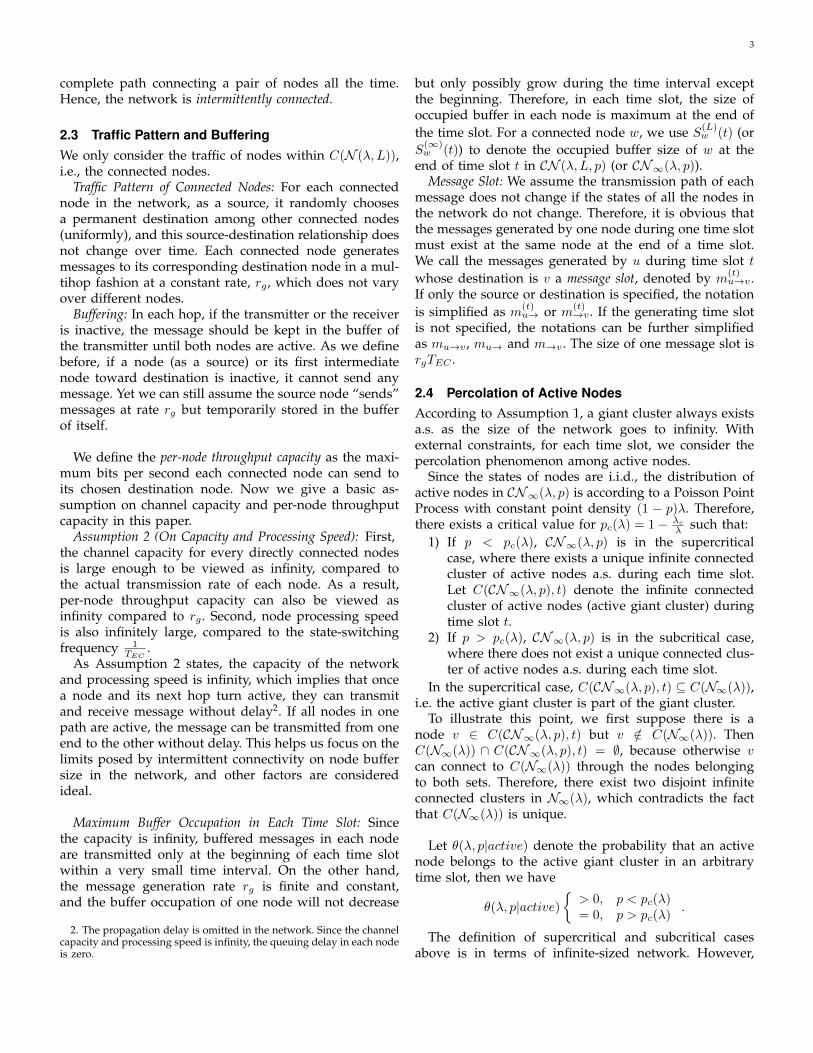
The time-domain variation of buffer occupation can bereduced if we apply flow control for each path, i.e. tocontrol the amount of messages sent in one time slotof each hop. In the simulation of which the results areillustrated in Fig. 15, we restrict that in one time slot eachhop can transmit at most 30 message slots. Obviously,the time-domain variation is largely reduced. In most oftime slots, the maximum buffer occupation is 30, and inonly very few time slots when it is up to 60. This flowcontrol is in terms of one path, and if one node belongsto multiple paths, it applies a separate flow control forevery path. Hence, such path flow control does not reducethe throughput of the network. Therefore, one node canset a queue for each path it serves for, to prevent toosmall non-empty ratio and too large buffer occupation ina particular time slot.
The discussions above shows that the Θ(√n) bound
3 10 20 50 100 300
1.4
1.6
1.8
2
2.2NE(2-path)n
NE(1-path)n
1
1.5
2
2.5
3NE(3-path)n
NE(1-path)n
3 10 20 50 100 300
Fig. 14. Multiple paths shared 3 nodes. p = 0.5.
can well reflect the actual buffer occupation even if wetake into consideration the variations in time domain.
5 DISCUSSIONS
5.1 On the Length of Time SlotWith the infinite channel capacity assumption, resultsin both supercritical and subcritical case indicate thatbuffer size requirements for connected nodes are closelyrelated to the length of time slot TEC . TEC determines thefrequency that the external constraints change, and theperiod a node being active or inactive. Results demon-strated in Theorems 1 and 2 show that minimum buffersize requirements for connected nodes are proportionalto the value of TEC .
This indicates that, without decreasing the probabilityof inactivity p, we can still reduce the requirements onbuffer size by making TEC smaller, if it is controllable. Forinstance, in a large scale wireless sensor network wherenode sleeping is allowed for saving energy, the amountof messages a node buffers can be reduced by making thesleeping and active periods smaller, even if their ratio isconstant. If we do not consider the power consumed byswitching between sleeping and active states, the powerconsumption for each node is mainly determined bythe ratio of the durations of sleeping and active states.Therefore, smaller periods do not impair the performanceof the energy saving mechanism.
Consider a network where buffer size of each node islimited, and TEC is controllable. Also assume the channel
12
5000 100000
50Node 1
5000 100000
50
100Node 161
5000 100000
20
40
60Node 641
5000 100000
20
40
60Node 801
0 100 200 300 400 500 600 700 80010
−2
10−1
100
Non-e
mpty
Rat
io
Node No.
t t
tt
Fig. 15. Time-domain variation with path flow control,p = 0.5, in one time slot each hop can transmit at most30 message slots.
capacity can be viewed as infinity due to the low messagegeneration rate rg , and the probability of inactivity p isrelatively large that the network is in the subcritical case.If it is required to support a constant rg as the size of thenetwork increases, we can scale TEC to O( 1√
n) to assure
limited buffer size of each node is enough.Further consider an extreme case where TEC → 0,
then buffer occupation also reduces to 0. This case issimilar to a TDMA scheme, and is equivalent that nodesare always active but channel capacity C reduces to aconstant proportion (1− p)2C. However, when TEC isvery small, the node processing speed can no longerbe viewed as infinity, and node inactivity caused byexternal factors (or constraints) are no longer crucial tothe network. In this case, internal factors such as capacityand processing speed are the main constraints of thenetwork performance.
By contrast, if TEC is not controllable and also nodebuffer size is limited, in the subcritical case, rg cannotremain constant as the size of the network increases. Inthis case, rg is at most Θ( 1√
n). This is the constraints on
rg even if the channel capacity is infinite.
5.2 On Finite Channel Capacity
Previous sections are based on the assumption of infinitechannel capacity due to the comparatively low messagegeneration rate, rg. Now we are going to discuss howthe results are applied to networks with finite channel
capacity. We again omit the processing delay of eachnode.
In both supercritical and subcritical case, each con-nected node on average serves as an intermediate forΘ(
√n) source-destination pairs, and thus the throughput
capacity of each node is Θ( 1√n). Similar and detailed
analysis of throughput capacity can be found in [17].The order of this throughput capacity is still achievableeven if node inactivity exists. Therefore, rg cannot remainconstant as n increases. Let rg = O( 1√
n), and we show that
Theorems 1 and 2 still hold.1) In the supercritical case, a message slot with size
rgTEC = O( 1√n) can be sent through Θ(
√n) hops
within constant time. Then we can still assure thebuffering path of each message consists of finitehops, and the existing time (delay) is still of constantorder. Therefore, the number of message slots eachnode needs to buffer is still of constant order, andthe size of buffered messages in one node is O( 1√
n).
Since the throughput capacity is Θ( 1√n), the buffered
messages does not exceed the order of the per-node throughput. Therefore, Theorem 1 still holds.Further, since rg = O( 1√
n), the actual amount of
buffered message in each connected node is alsoO( 1√
n).
2) In the subcritical case, the result in Theorem 2still holds if only rg does not exceed the per-nodethroughput capacity. With rg = O( 1√
n), the actual
amount of buffered message in each connected nodeis Θ(
√nrg) = O(1).
The discussion above show that when the channelcapacity is finite, and rg is adjusted according to the per-node throughput capacity, minimum occupied buffer sizeof each connected node does not increase with the growthof the network size.
6 USEFUL RESULTS ABOUT VACANT COMPO-NENTS IN SUPERCRITICAL CASE
A vacant component isolates the area inside it fromaccessing to the nodes outside. In supercritical case,vacant components cannot be very large.
Lemma 5: Randomly select a vacant component V inthe following way: first, uniformly randomly choose apoint o in R2; second, if o is not covered by any node,then let V = V {o} (the vacant component o belongs to),else return to the first step. (A larger vacant componentare more likely to be chosen.) If λ > λc (or (1− p)λ > λc
if only active nodes are considered) 6, then
P (d(V ) ≥ a) ≤ cv1e−cv2a,
6. If one only considers active nodes in one time slot, then in super-critical case it is (1 − p)λ > λc. So does that apply to Lemma 6 andCorollary 1.

13
where cv1, cv2 are constants with cv1 < ∞ and cv2 > 0.Proof: According to an immediate consequence of
Lemma 4.4 in [14] (on Page 114, above Corollary4.1), since in the supercritical case λ > λc, we haveσ∗(m, 3m, 1) → 0 (or σ∗(3m,m, 2) → 0) as m → ∞, whereσ∗(m, 3m, 1) (or σ∗(3m,m, 2)) is the probability for theexistence of a vacant crossing from left to right (or topto bottom) in a (m, 3m) (or (3m,m)) sized rectangular.Hence, we can find κ0 > 0 and large enough m such that
σ∗(m, 3m, 1) < κ0,
σ∗(3m,m, 2) < κ0.
Consider a randomly selected point o in R2, accordingto Lemma 4.1 in [14], we have
P (d(V {o}) ≥ a) ≤ c′v1e−c′v2a,
where V {o} is the vacant component containing o(d(V {o}) = 0 if o is covered by an active node), and c′v1,c′v2 are constants with c′v1 < ∞ and c′v2 > 0. And
P(d(V {o}) ≥ a))
= P(d(V {o}) ≥ a|d(V {o}) = 0))P(d(V {o}) = 0)
+P(d(V {o}) ≥ a|d(V {o}) > 0)P(d(V {o}) > 0)
= 0 + P(d(V {o}) ≥ a|d(V {o}) > 0)Pvac,
where Pvac is the proportion of space not covered bynodes, which is a constant when the node density isgiven.
Recall the way that V is selected, we have
P (d(V ) ≥ a) = P(d(V {o} ≥ a|d(V {o}) > 0)
=P(d(V {o} ≥ a))
Pvac≤ cv1e
−cv2a,
where cv1, cv2 are constants with cv1 < ∞ and cv2 > 0.Based on Lemma 5, we have the following result that
indicates a large area is not likely to be isolated by avacant component.
Lemma 6: Consider a randomly located line segmentwith length l, denoted by Sg(l). If λ > λc (or (1−p)λ > λc
if only considering active nodes), then the probability thatit is circulated by a vacant component is
P (Sg(l) is circulated by a vacant component) ≤ βe−αl,
where α, β are constants with β < ∞ and α > 0.Proof: As shown in Fig. 16, we draw a string of unit
squares, beginning at one endpoint of Sg(l) along theextended ray, denoted by {Sqi}. If a vacant componentcirculates Sg(l), then it has to intersect the extendedray. Let Ni denote the number of vacant componentsintersecting Sqi, and Vi,j (1 ≤ j ≤ Ni) denote the j-thvacant component intersecting Sqi. By Lemma 4.5 in [14],the expected number of vacant components intersectingeach square is a constant, denoted by Nvac = E(Ni).
Vacant
component
Sg(l)
Diameter of the vacant component
Sq1Sq2Sq3
Fig. 16. A line segment surrounded by a vacant compo-nent.
Since it is supercritical case, according to Lemma 5, wehave
P(Sqi contains a vacant component
with diameter larger than r)
≤∞∑k=0
P(Ni = k)k∑
j=1
P (d(Vi,j) ≥ r)
≤∞∑k=0
P(Ni = k)kcv1e−cv2r = cv1Nvace
−cv2r.
Further,
P (Sg(l) is circulated by a vacant component)
≤∞∑i=1
P(Sqi contains a vacant component
surroundsSg(l))
≤∞∑i=1
P(Sqi contains a vacant component
with diameter larger than l + i− 1)
≤∞∑i=1
cv1Nvace−cv2(l+i−1) ≤ βe−αl,
where α and β are constants with α > 0 and β < ∞.
Corollary 1: Consider a randomly located node w. Ifλ > λc (or (1 − p)λ > λc if only considering activenodes), then the probability that it is circulated by avacant component with diameter larger than l (denotedby the event EV (d>l)(w)) is
P(EV (d>l)(w)) ≤ β′(l + 1)e−α′l,
where α′, β′ are constants with β′ < ∞ and α′ > 0.Proof: We draw a horizonal ray starting from w, then
any vacant component that circulates w must intersect

14
this ray. The first segment with length l on this ray is de-noted by Sg(l). Similar as in the proof of Lemma 6, thereare a string of unit squares starting from the endpointof Sg(l). The number of vacant components intersectingwith Sg(l) is denoted by Nl, and E(Nl) < Nvacl. The setof such vacant components intersecting with Sg(l) is V lj .
possible vacant component
intersects within Sg(l)
possible vacant component
intersects outside Sg(l)
Sq1
Sq2
Sq3
wl
Sg(l)
Fig. 17. Possible vacant components circulate w withdiameter larger than l.
P(EV (d>l)(w))
≤∞∑k=0
P(Nl = k)k∑
j=1
P(d(V lj) > l)
+∞∑i=1
P(Sqi contains a vacant component
with diameter larger than l + i− 1)
≤ Nvaclcv1e−cv2l + βe−αl
≤ β′(l + 1)e−α′l,
where α′, β′ are constants with β′ < ∞ and α′ > 0.
7 CONCLUSION
In this paper, we have studied the fundamental lowerbound on node buffer size in intermittently connectedwireless networks where node inactivity is possible dueto external constraints. In detail, we analyzed bufferoccupation when the channel capacity is infinite, and theresults can be viewed as a lower bound for networkswith finite channel capacity. We find when the probabilityof inactivity is smaller than a critical value and thusthe network is in the supercritical case, the fundamentalachievable lower bound on node buffer size is Θ(1), i.e.the minimum node buffer size requirements are asymp-totically independent of the size of the network; when theprobability of inactivity is larger than the critical value,the network is in the subcritical case, and the achievablelower bound on node buffer size increases as the networkexpands, with the order of Θ(
√n).
We find since node buffer size requirements are propor-tional to the length of time slot according to which theexternal constraints changes, these requirements could be
reduced by decreasing the length of time slot, even if theprobability of inactivity remains unchanged.
We also find when the channel capacity is finite, andmessage generation rate is adjusted according to the per-node throughput capacity, results with infinite channelcapacity still hold.
REFERENCES[1] P. Gupta and P. R. Kumar,“The Capacity of Wireless Networks,”
IEEE Transactions on Information Theory, vol. 46, no. 2, pp. 388-404,March 2000.
[2] K. Fall, “A delay-tolerant network architecture for challengedInternets,” Proc. ACM SIGCOMM, pp. 27-34, 2003.
[3] A. Balasubramanian, B. N. Levine, A. Venkataramani, “DTN rout-ing as a resource allocation problem,” ACM SIGCOMM, pp. 373-384, 2007.
[4] Uichin Lee, Soon Young Oh, Kang-Won Lee, Mario Gerla, “ScalingProperties of Delay Tolerant Networks with Correlated MotionPatterns” ACM MobiCom Workshop on Challenged Networks (Chants2009), Beijing, China, September 25, 2009.
[5] W. Zhao, Y. Chen, M. Ammar, M. Corner, B. Levine, E. Zegura,“Capacity Enhancement using Throwboxes in DTNs,” IEEE Inter-national Conference on Mobile Adhoc and Sensor Systems (MASS),2006.
[6] T. Spyropoulos, K. Psounis, and C. Raghavendra, “Efficient Rout-ing in Intermittently Connected Mobile Networks: The Single-copyCase,” IEEE/ACM Transactions on Networking, Vol. 16, Iss. 1, pp. 63-76, February 2008.
[7] T. Spyropoulos, K. Psounis, and C. Raghavendra, “Efficient Rout-ing in Intermittently Connected Mobile Networks: The Multi-copyCase,” IEEE/ACM Transactions on Networking, Vol. 16, Iss. 1, pp.77-90, February 2008.
[8] O. Dousse, P. Mannersalo and P. Thiran, “Latency of wirelesssensor networks with uncoordinated power saing mechanisms,”Proc. ACM MobiHoc’04, May. 2004.
[9] W.Ren, Q.Zhao, and A.Swami, “On the Connectivity and Multi-hop Delay of Ad Hoc Cognitive Radio Networks,” Proc. of IEEEInternational Conference on Communications(ICC), May, 2010.
[10] Z. Kong and E. M. Yeh, “On the Latency for Information Dis-semination in Mobile Wireless Networks,” Proc. ACM MobiHoc’08,Hong Kong SAR, China, May. 2008.
[11] Jeffrey D. Herdtner and Edwin Chong, “Throughput-StorageTradeoff in Ad Hoc Networks,” IEEE INFOCOM, 2005.
[12] S. Bodas, S. Shakkottai, L. Ying and R. Srikant, “Schedulingin Multi-Channel Wireless Networks: Rate Function Optimalityin the Small-Buffer Regime,” proceedings of the ACM SIGMET-RICS/Performance Conference, June 2009.
[13] G. R. Grimmett, Percolaiton, Springer, 1999.[14] R. Meester and R. Roy, Continuum Percolation, NewYork: Cam-
bridge University Press, 1996.[15] M. Penrose, Random Geometric Graphs. New York: Oxford Univer-
sity Press, 2003.[16] T. M. Liggett, “An improved subadditive ergodic theorem,” The
Annals of Probability, vol. 13, no. 4, pp.1279C1285, 1985.[17] M. Franceschetti, O. Dousse, D. Tse and P. Thiran, “Closing the
gap in the capacity of wireless networks via percolation theory,”IEEE Trans. Inf. Theory, vol. 53, no. 3, pp. 1009-1018, Mar. 2007.
[18] C. Hu, X. Wang, D. Nie, J. Zhao, “Multicast Scaling Laws withHierarchical Cooperation,” in Proc. of IEEE INFOCOM 2010, SanDeigo, USA, 2010.
[19] C. Hu, Xinbing Wang, F. Wu, “MotionCast: On the Capacity andDelay Tradeoffs,” in ACM MobiHoc 2009, New Orleans, May 2009.
[20] Y. Liu, K. Liu, Mo Li, “Passive Diagnosis for Wireless SensorNetworks,” IEEE/ACM Transactions on Networking (TON), Vol. 18,No. 4, August 2010, Pages 1132-1144.
[21] Y. Liu, Y. He, Mo Li, et. al., “Does Wireless Sensor Network Scale?A Measurement Study on GreenOrbs,” IEEE INFOCOM, Shanghai,April 2011.