remote sensing

Article

Fully Automated Countrywide Monitoring of FuelBreak Maintenance Operations

Valentine Aubard 1,* , João E. Pereira-Pires 2 , Manuel L. Campagnolo 1 ,José M. C. Pereira 1 , André Mora 2 and João M. N. Silva 1

1 Forest Research Centre, School of Agriculture, University of Lisbon, Tapada da Ajuda, 1349-017 Lisbon,Portugal; mlc@isa.ulisboa.pt (M.L.C.); jmcpereira@isa.ulisboa.pt (J.M.C.P.);joaosilva@isa.ulisboa.pt (J.M.N.S.)

2 Centre of Technology and Systems/UNINOVA, School of Science and Technology—NOVA University ofLisbon, 2829-516 Caparica, Portugal; je.pires@campus.fct.unl.pt (J.E.P.-P.); atm@uninova.pt (A.M.)

* Correspondence: vaubard@isa.ulisboa.pt; Tel.: +336-29-27-35-22

Received: 4 August 2020; Accepted: 2 September 2020; Published: 5 September 2020�����������������

Abstract: Fuel break (FB) networks are strategic locations for fire control and suppression. In order tobe effective for wildfire control, they need to be maintained through regular interventions to reducefuel loads. In this paper, we describe a monitoring system relying on Earth observations to detect fuelreduction inside the FB network being implemented in Portugal. Two fast automated pixel-basedmethodologies for monthly monitoring of fuel removals in FB are developed and compared. The firstmethod (M1) is a classical supervised classification using the difference and postdisturbance image ofmonthly image composites. To take into account the impact of different land cover and phenologyin the detection of fuel treatments, a second method (M2) based on an innovative statistical changedetection approach was developed. M2 explores time series of vegetation indices and does not requiretraining data or user-defined thresholds. The two algorithms were applied to Sentinel-2 10 m bandsand fully processed in the cloud-based platform Google Earth Engine. Overall, the unsupervisedM2, which is based on a Welch t-test of two moving window averages, gives better results than thesupervised M1 and is suitable for an automated countrywide fuel treatment detection. For bothmethods, two vegetation indices, the Modified Excess of Green and the Normalized DifferenceVegetation Index, were compared and exhibited similar performances.

Keywords: fuel load; vegetation monitoring; wildfire prevention; change detection; remote sensing;time series; Sentinel-2

1. Introduction

As highlighted by the Australian 2019 fire disaster and large wildfires in California, Swedenor Portugal in recent years, fire regimes are evolving at a high rate [1]. Climate change enhancesthe risk and severity of wildfires, by favoring the frequency and combination of extreme events:extended periods of high temperatures, droughts and high wind speed. Simulations suggest that firedanger, catalyzed by climate, is going to increase for all European countries by 2100, particularly inMediterranean areas [2].

Portugal is the most fire-prone of all European countries [3]. Although there are contrastingregions in terms of burned area trends [4], the country presents a global positive trend of annualburned area for 2001–2017 despite an increasing investment in fire suppression means [5]. The mainreason is a general abandonment of rural areas and a lack of management of agricultural lands andforests, resulting in high fuel load and shrub encroachment [4,6]. These unsustainable managementpractices and a high rate of anthropogenic ignition sources, coupled with favorable climate conditions,

Remote Sens. 2020, 12, 2879; doi:10.3390/rs12182879 www.mdpi.com/journal/remotesensing

Remote Sens. 2020, 12, 2879 2 of 18

will lead to a severe increase in large fires in future decades. Recently, Portugal policymakers decidedto invest in landscape-level fuel management [7], especially with a new fuel break linear networkwhose implementation and maintenance are coordinated by the Portuguese Institute for Nature andForests Conservation (ICNF).

Fuel breaks (FB) are commonly defined as areas of any shape and size where fuel loads arefrequently reduced. They are located in strategic places of fire combat, typically alongside ridges andwater lines, which efficiently allow firefighters to access suppression places, stop the propagation of afire, or at least significantly decrease its burned area [8,9]. Easy access to FB improves significantlyfirefighting efficiency [8], thus a road commonly passes through its center. As specified in Section 4of [10], the FB of the Portuguese primary network should have a minimum width of 125 m. Accordingto the technical specifications, the tree cover should gradually decrease from the outside border to themiddle, to ensure the horizontal discontinuity of the tree stratum (Figure 1). Lower branches are prunedand the understory suppressed regularly to ensure the vertical fuel discontinuity. The innermost 10 mon each side of the road have their vegetation totally removed (herbaceous, shrubs and trees). Rainfedagricultural fields included in the FB should be harvested before the summer season. This technicalmodel is adapted to local conditions.

Remote Sens. 2020, 12, x FOR PEER REVIEW 2 of 19

conditions, will lead to a severe increase in large fires in future decades. Recently, Portugal policymakers decided to invest in landscape-level fuel management [7], especially with a new fuel break linear network whose implementation and maintenance are coordinated by the Portuguese Institute for Nature and Forests Conservation (ICNF).

Fuel breaks (FB) are commonly defined as areas of any shape and size where fuel loads are frequently reduced. They are located in strategic places of fire combat, typically alongside ridges and water lines, which efficiently allow firefighters to access suppression places, stop the propagation of a fire, or at least significantly decrease its burned area [8,9]. Easy access to FB improves significantly firefighting efficiency [8], thus a road commonly passes through its center. As specified in Section 4 of [10], the FB of the Portuguese primary network should have a minimum width of 125 m. According to the technical specifications, the tree cover should gradually decrease from the outside border to the middle, to ensure the horizontal discontinuity of the tree stratum (Figure 1). Lower branches are pruned and the understory suppressed regularly to ensure the vertical fuel discontinuity. The innermost 10 m on each side of the road have their vegetation totally removed (herbaceous, shrubs and trees). Rainfed agricultural fields included in the FB should be harvested before the summer season. This technical model is adapted to local conditions.

Figure 1. Transversal view of a model fuel break. The total width is 125 m. The distance between tree crowns decreases with the distance to the road. The first 10 m on the sides of the road have no vegetation. Adapted from [10].

Once the FB is created, frequent interventions are needed to reduce fuel loads. They are performed mainly by mechanical fuel removal and, less frequently, by prescribed fire or grazing. Fuel reduction treatments are made at any time of the year, even though they are unadvised during the fire season, from June to October. Municipalities are responsible for FB maintenance on their territory [11], but national institutions, such as ICNF and Civil Protection, need to know the dates and locations of fuel treatment for planning safe and efficient emergency actions, for evaluating and adapting policy [8,9]. They need a cheap, fast and easy-to-use method to obtain this information every year, for the whole country.

A large variety of change detection techniques exists for passive remote-sensing data. The more classical approach is hybrid methods, for example, simple arithmetic operations (e.g., differencing) followed by a supervised or unsupervised classification [12,13]. Classifications usually require an accurate and diversified training dataset [14]. For the specific case of binary changes (change or no change), another successful technique is to detect changes based on user-defined thresholds, on ”one-shot” differences or time series, which can be interpolated for comparison [15–17]. However, this requires a good empirical knowledge of the change signal and duration, which is not feasible in this study due to the diversity of climate, soil, species and vegetation phenology responses and land use types present in FB [18]. Object-based detections have the advantage to use spatial information but require a reliable segmentation, which limits their utility in the case of FB, where fuel treatments may have variable geometries over the years [19]. The Copernicus Sentinel-2 multispectral instrument (S2) from the European Space Agency (ESA) [20] has its first four bands at 10 m resolution and, since the launch of a second satellite in 2017, a 5 day revisit period. This new sensor allows the detection of vegetation changes within narrow structures such as FB.

Figure 1. Transversal view of a model fuel break. The total width is 125 m. The distance betweentree crowns decreases with the distance to the road. The first 10 m on the sides of the road have novegetation. Adapted from [10].

Once the FB is created, frequent interventions are needed to reduce fuel loads. They are performedmainly by mechanical fuel removal and, less frequently, by prescribed fire or grazing. Fuel reductiontreatments are made at any time of the year, even though they are unadvised during the fire season,from June to October. Municipalities are responsible for FB maintenance on their territory [11],but national institutions, such as ICNF and Civil Protection, need to know the dates and locationsof fuel treatment for planning safe and efficient emergency actions, for evaluating and adaptingpolicy [8,9]. They need a cheap, fast and easy-to-use method to obtain this information every year,for the whole country.

A large variety of change detection techniques exists for passive remote-sensing data. The moreclassical approach is hybrid methods, for example, simple arithmetic operations (e.g., differencing)followed by a supervised or unsupervised classification [12,13]. Classifications usually require anaccurate and diversified training dataset [14]. For the specific case of binary changes (change orno change), another successful technique is to detect changes based on user-defined thresholds,on “one-shot” differences or time series, which can be interpolated for comparison [15–17]. However,this requires a good empirical knowledge of the change signal and duration, which is not feasible inthis study due to the diversity of climate, soil, species and vegetation phenology responses and landuse types present in FB [18]. Object-based detections have the advantage to use spatial information butrequire a reliable segmentation, which limits their utility in the case of FB, where fuel treatments mayhave variable geometries over the years [19]. The Copernicus Sentinel-2 multispectral instrument (S2)from the European Space Agency (ESA) [20] has its first four bands at 10 m resolution and, since thelaunch of a second satellite in 2017, a 5 day revisit period. This new sensor allows the detection ofvegetation changes within narrow structures such as FB.

Remote Sens. 2020, 12, 2879 3 of 18

The goal of this work is to develop a monitoring system based on remotely sensed data forfuel treatments in a Portuguese FB network, i.e., a system that allows the detection of where andwhen (with a monthly precision) treatments occurred in FB network. This study answers to threescientific challenges: (i) detecting changes in 125 m wide narrow spatial features; (ii) dealing withregions with differences in climate, soil and land cover; (iii) developing a semi/fully automated process.Two pixel-based methodologies were developed to fulfill this task: a supervised classification basedon monthly image composites and a statistical approach that takes advantage of the exhaustiveinformation contained in multispectral time series of satellite data. The second method does not requirea specific training data set, nor predefined thresholds. The two algorithms were applied to S2 10 mbands and fully processed in the cloud-based platform Google Earth Engine (GEE) [21], which allowsthe future application of the methodology to other Mediterranean regions.

This paper first presents the data used and the two methodologies developed. Results are givenfor five study sites in mainland Portugal. The last section discusses results and compares the twomethods performances.

2. Materials and Methods

2.1. Data

2.1.1. Portuguese Land Use and Land Cover Map

The land use and land cover (LULC) map is a thematic vector map for mainland Portugal, based onphotointerpretation of orthorectified areal images [22]. It delineates homogenous areas (polygons),with a minimum mapping unit of 1 ha, in which at least 75% of the surface belongs to the same LULCclass. This map gives a precise 5-level hierarchical classification with 48 classes in the most detailedlevel. This classification was simplified to suit this work’s methodology and objectives (Table 1).

Table 1. Simplified land cover classification, adapted from [22], with area and relative area in thePortuguese fuel break network.

Name Original ClassNumber Details Area (ha) Relative Area (%)

Artificialized lands 1.

Continuous and discontinuousurban fabric, industries, parks,airports, historical areas, leisureinfrastructures and golf fields.

1747 3.6

Agriculture 2.

Permanent and temporaryagriculture fields, some withnatural areas, includingorchards, olive groves andvineyards.

5497 11.4

Forest 3.1.Mainly cork oaks, holm oaks,eucalyptus, stone pine andmaritime pine.

24,017 49.7

Agroforestry 2.4.4. Oaks or pines agroforestrysystems. 663 1.4

Shrublands 3.2.2. 13,621 28.2

Herbaceousvegetation 2.3. and 3.2.1. Permanent pasture and natural

herbaceous 1869 3.9

Sparse vegetation 3.3. 787 1.6

Water 4. and 5. Inland water and wetlands 145 0.3

Total 48,346 100

Remote Sens. 2020, 12, 2879 4 of 18

According to the 2015 LULC map, the main land cover classes present in the FB are forests (50%)and shrublands (28%) (Table 1). Forests are mainly composed of evergreen species (pine, eucalypt,cork oak and holm oak) which display stable spectral reflectance signals along the year. On the otherhand, shrubs and herbaceous vegetation show strong phenological variations, hardly predictable fromone year to the following as they depend on the species, the soil and the meteorological conditions [23].The third main land cover class is agriculture (11%), which is, by far, the more diversified category interms of land cover species and management.

2.1.2. Study Sites

Five areas distributed in mainland Portugal (Figure 2) were chosen as a representative subset ofPortugal diversity in terms of land cover (according to the 2015 LULC map) and climate conditions(Table 2). Mainland Portugal is divided into two temperate climate regions according to the Köppenclassification: the southeastern part has a hot-summer Mediterranean climate with rainy winters andhot dry summers (Csa, Serra de Caldeirão area), while the northwestern part has a warm-summerMediterranean climate with rainy winters and warm dry summers (Csb, Amarante and Manteigas).Serra de Candeeiros and Proença-a-Nova are at the confluence of the two climate zones. Differentyears were studied, as a function of the dates of the fuel management operations, which adds to thevariability of the climate conditions.

Remote Sens. 2020, 12, x FOR PEER REVIEW 4 of 19

Herbaceous vegetation

2.3. and 3.2.1.

Permanent pasture and natural herbaceous

1869 3.9

Sparse vegetation

3.3. 787 1.6

Water 4. and 5. Inland water and wetlands 145 0.3 Total 48,346 100

2.1.2. Study Sites

Five areas distributed in mainland Portugal (Figure 2) were chosen as a representative subset of Portugal diversity in terms of land cover (according to the 2015 LULC map) and climate conditions (Table 2). Mainland Portugal is divided into two temperate climate regions according to the Köppen classification: the southeastern part has a hot-summer Mediterranean climate with rainy winters and hot dry summers (Csa, Serra de Caldeirão area), while the northwestern part has a warm-summer Mediterranean climate with rainy winters and warm dry summers (Csb, Amarante and Manteigas). Serra de Candeeiros and Proença-a-Nova are at the confluence of the two climate zones. Different years were studied, as a function of the dates of the fuel management operations, which adds to the variability of the climate conditions.

Figure 2. Locations of the five study areas in Portugal.

Table 2. Study sites studied years, fuel break area, land cover composition and climate conditions.

Study Area Years Area (ha) Forest (%) Shrubs (%) P (mm) * maxT (°C) * Serra de Caldeirão 2016–2017 205.2 58.7 40 800 19 Manteigas 2016–2017 204.6 31 42.2 1400 14 Serra de Candeeiros 2017–2018 398.6 20.9 61.9 1200 18 Amarante 2018–2019 97.6 90.3 8.3 1600 16 Proença-a-Nova 2018–2019 202 79.2 19.2 1100 20 Total 2016–2019 1108 46.5 41.7

Figure 2. Locations of the five study areas in Portugal.

Remote Sens. 2020, 12, 2879 5 of 18

Table 2. Study sites studied years, fuel break area, land cover composition and climate conditions.

Study Area Years Area (ha) Forest (%) Shrubs (%) P (mm) * maxT (◦C) *

Serra deCaldeirão 2016–2017 205.2 58.7 40 800 19Manteigas 2016–2017 204.6 31 42.2 1400 14Serra deCandeeiros 2017–2018 398.6 20.9 61.9 1200 18Amarante 2018–2019 97.6 90.3 8.3 1600 16Proença-a-Nova 2018–2019 202 79.2 19.2 1100 20Total 2016–2019 1108 46.5 41.7

* Mean annual precipitation (P) and maximum temperature (maxT) based on the 1971–2000 climate normals(source: IPMA).

2.1.3. Imagery and Choice of Indices

Free-access satellite imagery at a medium/high spatial resolution and short revisit time offer a highpotential for the efficient detection of fuel removal interventions within the FB. However, the detectionis expected to be more difficult for understory vegetation than in treeless areas. Thus, it was primordialto obtain a clear signal from the innermost 10 m on each side of the central road, which is devoid oftrees, by design: considering the entire FB width of 125 m, only around ten pure pixels of 10 m size areavailable, i.e., free from a mixture of spectral signals from the middle road or the FB boundary. It wasdecided to use only the first four bands of the S2 MSI products, the visible bands B4, B3 and B2 andthe near-infrared (NIR) band B8, which have a spatial resolution of 10 m and a temporal resolution of5 days since March 2017. Two processing levels of S2 images are available in GEE: ortho-images withTop of Atmosphere reflectance (TOA, level-1C); after April 2017, atmospherically corrected Bottom ofAtmosphere reflectance (BOA, level-2A) images, calculated with the Sen2Cor processor [20]. In thiswork, we used TOA images, for their abundance (a key aspect for time series approach) and theiravailability before 2017.

We limited our analysis to two vegetation indices, calculated with S2 TOA 10 m bands to detectsudden decreases in fuel cover: the Normalized Difference Vegetative Index (NDVI) [24]:

NDVI = (NIR − R) / (NIR + R), (1)

meaningful, efficient and widely used in remote sensing applications and the Modified Excess of Green(MExG) [25,26]:

MExG = 1.262 G − 0.884 R − 0.311 B, (2)

based on visible bands, efficient to discriminate vegetation from soil and robust to changingillumination conditions.

2.2. Two Methodologies for Fuel Break Monitoring

Two complementary methodologies were developed to deal with the phenology of vegetation,the unavailability of reliable training data and the scarcity of clear images (cloud-free and cloudshadow-free). The first method (M1) is based on a pixel-based supervised classification, using monthlycomposite images differences. The monthly step can be adapted in case of severe unavailability ofclear imagery. The second method (M2), computationally more demanding, is based on the detectionof statistically significant differences across the time series of satellite data, using a moving windowon each pixel. It does not need training data since it uses as a reference the outside neighborhoodarea of the FB. By these means, it is supposed to avoid false positives due to phenological variations.Imperfect cloud or shadow masking and/or the lack of data are limitations for this technique, since itrelies on a statistical test performed on dense time series.

Remote Sens. 2020, 12, 2879 6 of 18

Preprocessing, common to both methods, and processing, specific to each one, were performed inthe JavaScript application programming interface (API) of GEE, taking advantage of its powerful cloudinterface and computational speed. The workflow (Figure 3) summarizes the main steps described inthe following sections.

Remote Sens. 2020, 12, x FOR PEER REVIEW 6 of 19

Figure 3. Flowchart including the common preprocessing and the two methodologies.

2.2.1. Common Preprocessing

To mask S2 TOA clouds, cloud shadows and snow, the thresholds and vegetation indices used in the Sen2Cor algorithm [27] were implemented in GEE. S2 TOA images are already georeferenced and their bands aligned [20]. However, some small shifts up to 15 m exist, especially between images from different satellites, which means that images need to be coregistered. If this error is not corrected, pixels in the borders or in the middle road of the FB may shift multiple times from vegetation to no vegetation, increasing the risk of false positives. An image coregistration process was performed for each Sentinel tile and year. A reference image is automatically selected for being free-of-clouds, covering the whole tile, from satellite A (generally better registered according to FB limits) and with the closer date to 1 May. Then, the function displacement of GEE API, which explores pixel correlations [28] between the Red bands of each image and of the reference, was used to estimate the optimal displacement (final parameters used after some tests: maxOffset: 25; patchWidth: 50; stiffness: 5; bicubic resampling). Each band and vegetation index was finally realigned with the function displace (see an example in Figure 4).

Figure 3. Flowchart including the common preprocessing and the two methodologies.

2.2.1. Common Preprocessing

To mask S2 TOA clouds, cloud shadows and snow, the thresholds and vegetation indices usedin the Sen2Cor algorithm [27] were implemented in GEE. S2 TOA images are already georeferencedand their bands aligned [20]. However, some small shifts up to 15 m exist, especially between imagesfrom different satellites, which means that images need to be coregistered. If this error is not corrected,pixels in the borders or in the middle road of the FB may shift multiple times from vegetation to novegetation, increasing the risk of false positives. An image coregistration process was performedfor each Sentinel tile and year. A reference image is automatically selected for being free-of-clouds,covering the whole tile, from satellite A (generally better registered according to FB limits) andwith the closer date to 1 May. Then, the function displacement of GEE API, which explores pixelcorrelations [28] between the Red bands of each image and of the reference, was used to estimate theoptimal displacement (final parameters used after some tests: maxOffset: 25; patchWidth: 50; stiffness:

Remote Sens. 2020, 12, 2879 7 of 18

5; bicubic resampling). Each band and vegetation index was finally realigned with the function displace(see an example in Figure 4).Remote Sens. 2020, 12, x FOR PEER REVIEW 7 of 19

Figure 4. Time series A. before and B. after coregistration of three points located on an unpaved road of the fuel break (center, in blue), 20 m on its left (red) and 20 m on its right (orange), with C. the location of the three points on an aerial view of the fuel break. The images of the tile are all coregistered using a reference image (vertical dash line).

2.2.2. Method 1: Supervised Classification

We first created monthly maximum composites [29]. In GEE, it is possible to create a composite ”pixel by pixel” by transforming the image collection into an ”Array Image”, where each pixel becomes an Array (or table) with two dimensions: the images and the bands [30]. For each pixel, the images can then be sorted according to the value of one of the bands. We sorted each month collection according to the NDVI band and extracted (for each pixel) the image bands’ values (R, G, B, NDVI and MExG), for which NDVI was the highest. To reduce noise in the data, only images with a ”CLOUDY_PIXEL_PERCENTAGE” lower than 30% were used for compositing. The monthly maximum NDVI composites, unlike MExG maximum composites, proved to be an efficient way of enhancing fuel treatment signals and reducing clouds and shadows in the composites. We used the MExG band generated from the same maximum NDVI composite for the next steps of this method. Then, the difference of monthly composites was computed, allowing the detection of fuel treatments on FB (Figure 5).

Figure 4. Time series (A). before and (B). after coregistration of three points located on an unpavedroad of the fuel break (center, in blue), 20 m on its left (red) and 20 m on its right (orange), with (C).the location of the three points on an aerial view of the fuel break. The images of the tile are allcoregistered using a reference image (vertical dash line).

2.2.2. Method 1: Supervised Classification

We first created monthly maximum composites [29]. In GEE, it is possible to create a composite“pixel by pixel” by transforming the image collection into an “Array Image”, where each pixelbecomes an Array (or table) with two dimensions: the images and the bands [30]. For each pixel,the images can then be sorted according to the value of one of the bands. We sorted each monthcollection according to the NDVI band and extracted (for each pixel) the image bands’ values (R, G,B, NDVI and MExG), for which NDVI was the highest. To reduce noise in the data, only imageswith a “CLOUDY_PIXEL_PERCENTAGE” lower than 30% were used for compositing. The monthlymaximum NDVI composites, unlike MExG maximum composites, proved to be an efficient way ofenhancing fuel treatment signals and reducing clouds and shadows in the composites. We used theMExG band generated from the same maximum NDVI composite for the next steps of this method.Then, the difference of monthly composites was computed, allowing the detection of fuel treatmentson FB (Figure 5).

Remote Sens. 2020, 12, 2879 8 of 18Remote Sens. 2020, 12, x FOR PEER REVIEW 8 of 19

Figure 5. Example in Serra de Candeeiros (shrubs) of: (A) two monthly maximum NDVI

composites; (B) their difference (June composite–May composite).Training datasets were established using the information provided by ICNF on the location of fuel treatments, and also through visual image interpretation. The training dataset contains the values of 20,000 points inside and outside the FB, from all months of the year, one-third of which correspond to locations where fuel removal interventions occurred.

Two classifiers were used separately: Random Forest and Maximum Entropy (MaxEnt). Both classifiers predict the occurrence of fuel removal interventions given the vegetation indices values. Random Forest [31] generates a large number of decision trees by sampling the training dataset with replacement. To classify a new instance, it collects the classifications and chooses the most voted prediction as the result. MaxEnt estimates probability distributions over an extended feature space for positive events and for all events (background) and minimizes the relative entropy between those two distributions [32]. The ratio of the probability densities is then converted into a likelihood of occurrence for each instance.

Two images were used for training and classification: a vegetation index composite (postdisturbance value) and its difference to the previous monthly composite (disturbance absolute value). The result was a monthly binary intervention/no intervention (INI) classification.

2.2.3. Method 2: Time Series and Welch’s t-Test

Three time series were used: (a) for each vegetation index, the time series of each pixel located inside the FB, ”inside pixel”, was computed for one calendar year and elongated by two months, before and after, to encompass the two-month wide moving window that is necessary for the statistical test; (b) the neighboring pixels within 500 m, located outside the FB and of the same land cover class according to 2015 LULC map were used to calculate an ”outside mean” time series; (c) the ”difference” between those two times series was also computed. When images were from the same date, the maximum value of was kept. The outside mean series interquartile range detected and masked the remaining extreme values in the three series (unmasked clouds or shadows).

A one-sided Welch’s t-test was then applied to each date for the three time series [33]. This test is an adaptation of the Student’s t-test, allowing the identification of significant differences (only significant drops due to the one-sided imposition) between the means of two groups with different sizes and variances. Here, our groups were defined by two temporal moving windows—before and after each date. The minimum number of dates for the test was 2 on each side. We also defined a maximum of 8 dates, to limit the windows’ sample size difference, and a maximum window length of 60 days, to avoid comparing values too far apart but keep enough available dates (some months

Figure 5. Example in Serra de Candeeiros (shrubs) of: (A) two monthly maximum NDVI composites;(B) their difference (June composite–May composite).Training datasets were established using theinformation provided by ICNF on the location of fuel treatments, and also through visual imageinterpretation. The training dataset contains the values of 20,000 points inside and outside theFB, from all months of the year, one-third of which correspond to locations where fuel removalinterventions occurred.

Two classifiers were used separately: Random Forest and Maximum Entropy (MaxEnt).Both classifiers predict the occurrence of fuel removal interventions given the vegetation indicesvalues. Random Forest [31] generates a large number of decision trees by sampling the training datasetwith replacement. To classify a new instance, it collects the classifications and chooses the most votedprediction as the result. MaxEnt estimates probability distributions over an extended feature spacefor positive events and for all events (background) and minimizes the relative entropy between thosetwo distributions [32]. The ratio of the probability densities is then converted into a likelihood ofoccurrence for each instance.

Two images were used for training and classification: a vegetation index composite(postdisturbance value) and its difference to the previous monthly composite (disturbance absolutevalue). The result was a monthly binary intervention/no intervention (INI) classification.

2.2.3. Method 2: Time Series and Welch’s t-Test

Three time series were used: (a) for each vegetation index, the time series of each pixel locatedinside the FB, “inside pixel”, was computed for one calendar year and elongated by two months,before and after, to encompass the two-month wide moving window that is necessary for the statisticaltest; (b) the neighboring pixels within 500 m, located outside the FB and of the same land coverclass according to 2015 LULC map were used to calculate an “outside mean” time series; (c) the“difference” between those two times series was also computed. When images were from the same date,the maximum value of was kept. The outside mean series interquartile range detected and masked theremaining extreme values in the three series (unmasked clouds or shadows).

A one-sided Welch’s t-test was then applied to each date for the three time series [33]. This test is anadaptation of the Student’s t-test, allowing the identification of significant differences (only significantdrops due to the one-sided imposition) between the means of two groups with different sizes andvariances. Here, our groups were defined by two temporal moving windows—before and after eachdate. The minimum number of dates for the test was 2 on each side. We also defined a maximumof 8 dates, to limit the windows’ sample size difference, and a maximum window length of 60 days,

Remote Sens. 2020, 12, 2879 9 of 18

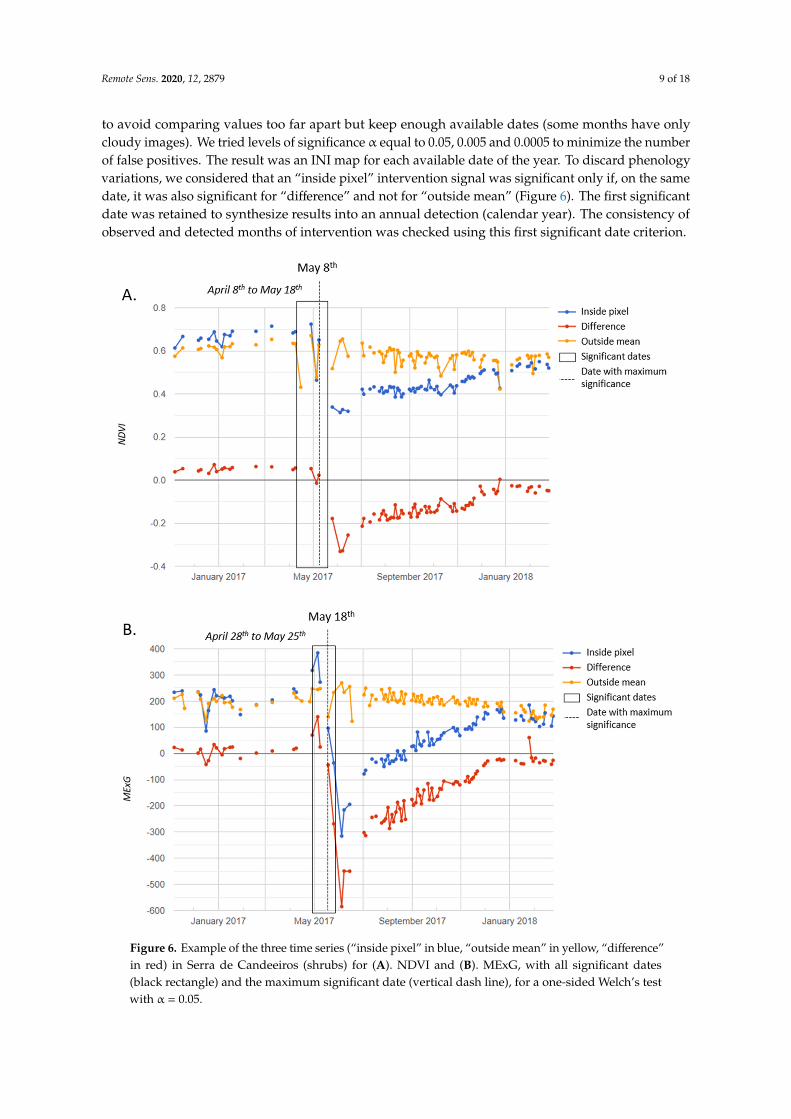
to avoid comparing values too far apart but keep enough available dates (some months have onlycloudy images). We tried levels of significance α equal to 0.05, 0.005 and 0.0005 to minimize the numberof false positives. The result was an INI map for each available date of the year. To discard phenologyvariations, we considered that an “inside pixel” intervention signal was significant only if, on the samedate, it was also significant for “difference” and not for “outside mean” (Figure 6). The first significantdate was retained to synthesize results into an annual detection (calendar year). The consistency ofobserved and detected months of intervention was checked using this first significant date criterion.

Remote Sens. 2020, 12, x FOR PEER REVIEW 9 of 19

have only cloudy images). We tried levels of significance α equal to 0.05, 0.005 and 0.0005 to minimize the number of false positives. The result was an INI map for each available date of the year. To discard phenology variations, we considered that an ”inside pixel” intervention signal was significant only if, on the same date, it was also significant for ”difference” and not for ”outside mean” (Figure 6). The first significant date was retained to synthesize results into an annual detection (calendar year). The consistency of observed and detected months of intervention was checked using this first significant date criterion.

Figure 6. Example of the three time series (”inside pixel” in blue, ”outside mean” in yellow, ”difference” in red) in Serra de Candeeiros (shrubs) for (A). NDVI and (B). MExG, with all significant dates (black rectangle) and the maximum significant date (vertical dash line), for a one-sided Welch’s test with α = 0.05.

Figure 6. Example of the three time series (“inside pixel” in blue, “outside mean” in yellow, “difference”in red) in Serra de Candeeiros (shrubs) for (A). NDVI and (B). MExG, with all significant dates(black rectangle) and the maximum significant date (vertical dash line), for a one-sided Welch’s testwith α = 0.05.

Remote Sens. 2020, 12, 2879 10 of 18

2.3. Validation and Results’ Comparison

Validation polygons were delimited for every month, using ground truth and visual imageinterpretation. Results fell into one of two categories: interventions in the FB were considered positiveevents (“Yes”) the first month they were observed as such; already treated and never treated areaswere considered negative events (“No” intervention).

Monthly INI 2x2 error matrices, which entries are TP the number of true positive events,TN standing for true negative, FP for false positive and FN for false negative events, were obtainedfrom both methods. To compare the methods’ results, suitable accuracy metrics were chosen: overallaccuracy, precision, recall and F1-score [30,31]. The overall accuracy expresses the proportion ofreferenced sites (validation pixels) that were mapped correctly in the dataset:

Overall accuracy = (TP + TN)/(TP + TN + FP + FN). (3)

Precision and recall metrics were computed for each category reflecting the occurrence of falsepositives and negatives. For one category (a fuel treatment detected, “Yes”, or no fuel treatment,“No”), the precision gave the fraction of correctly classified events among retrieved events, here for thecategory “Yes”:

Precision = TP/(TP + FP) = 1 − commission error. (4)

A higher precision meant that the classifier had a good behavior avoiding false positives events.Among one category, the recall measured the fraction of relevant events that was classified as such,for category “Yes”:

Recall = TP/(TP + FN) = 1 − omission error. (5)

The recall showed the ability of the classifier to not detect false negatives. The F1-score, that rangedbetween 0 (when either Precision or Recall is zero) and 1 (when both are 1), was a balance betweenprecision and recall that measured the accuracy of the classification of each category:

F1-score = 2 × (Precision × Recall)/(Precision + Recall) (6)

The accuracy of the methods was compared at two time steps. At the monthly step, the accuracymetrics were calculated from the sum of the twelve monthly INI error matrices from one year. For annualcomparisons, monthly maps were aggregated: a pixel observed or detected positive one or more timesduring the year was considered a positive event; if it was never detected positive, it stayed negative.Those annual binary maps of results and validations were used to compute annual INI error matricesand the corresponding accuracy metrics.

3. Results

Four classifier–vegetation index pairs were tested in M1. Table 3 compares the accuracy metricsfor each pair, at annual and monthly steps. Recall, Precision and F1-score metrics are given separatelyfor the two categories: positive events (fuel treatment detected: “Yes”) and negative events (“No”).Metrics revealed that MaxEnt performed better than RF, and NDVI better than MExG. The best couple,MaxEnt-NDVI, could detect fuel treatment with a 54% precision and 69% recall on a yearly basis.For positive events, the monthly F1-score was lower than the annual score (45% against 61%). A deeperanalysis of results revealed that this was mainly due to a difference of one or two months earlier orlater with regard to the validation date.

Two vegetation indices and three levels of significance were tested with M2 (Table 4). NDVI andMExG gave close results. For both, the precision tended to increase inversely to α, at the expense of therecall. The metrics showed an improved precision in comparison to the best pair of M1 (MaxEnt-NDVI),but a lower recall.

Remote Sens. 2020, 12, 2879 11 of 18

Table 3. Global accuracy results for Method 1, at annual and monthly steps.

Classifier and Index MaxEnt NDVI MaxEnt MExG RF NDVI RF MExG

Fuel treatment detected Yes No Yes No Yes No Yes No

Annual

Precision (%) 54 87 35 95 43 87 33 92Recall (%) 69 78 96 32 73 64 94 29

F1-Score (%) 61 82 51 48 54 74 49 44Overall accuracy (%) 75 50 66 46

Monthly

Precision (%) 38 99 8 99 25 99 11 99Recall (%) 56 98 83 78 55 96 63 87

F1-Score (%) 45 98 15 88 35 98 18 93Overall accuracy (%) 97 79 95 87

Table 4. Global accuracy results for Method 2, at annual and monthly steps.

Vegetation index andLevel of significance

NDVI0.05

NDVI0.005

NDVI0.0005

MExG0.05

MExG0.005

MExG0.0005

Fuel treatment detected Yes No Yes No Yes No Yes No Yes No Yes No

Annual

Precision (%) 37 87 56 83 74 80 35 83 50 83 66 82Recall (%) 80 50 57 83 40 95 77 45 60 76 47 91

F1-Score (%) 51 63 57 83 52 87 48 59 54 79 55 86Overall

accuracy (%) 58 76 79 54 72 79

Monthly

Precision (%) 10 98 26 98 52 98 10 98 27 98 45 98Recall (%) 21 96 27 98 28 99 23 95 33 98 32 99

F1-Score (%) 13 97 27 98 37 99 14 97 30 98 37 99Overall

accuracy (%) 94 97 98 94 96 98

The detection of positive FB treatments was less accurate in the forest areas than in shrublands,for both methods (Table 5). On the contrary, negative events lost accuracy in shrublands, potentiallybecause of higher phenological variations.

Table 5. Comparison of the accuracies obtained for two land cover types: Forest and Shrubs; for the pairMaxEnt-NDVI from Method 1 (M1) and the indices NDVI and MExG from Method 2 with α = 0.0005,at annual and monthly steps.

Land cover and Method Forest M1 ForestNDVI

ForestMExG Shrubs M1 Shrubs

NDVIShrubsMExG

Fuel treatment detected Yes No Yes No Yes No Yes No Yes No Yes No

Annual

Precision (%) 45 90 69 88 57 89 60 84 83 78 78 80Recall (%) 62 82 43 95 51 91 71 76 47 95 55 92

F1-Score (%) 52 86 53 91 54 90 65 80 60 86 6f4 86Overall

accuracy (%) 78 85 83 75 79 80

Monthly

Precision (%) 34 99 54 99 41 99 47 99 58 98 53 98Recall (%) 52 98 33 100 37 99 62 98 33 99 37 99

F1-Score (%) 41 99 41 99 38 99 53 98 42 99 44 99Overall

accuracy (%) 98 98 98 97 97 97

Figure 7 shows an example of map results for both methods in Serra de Aires, a shrubland. We cansee the improvement of M2 monthly detection results when α decreased (NDVI from α = 0.05 toα = 0.0005). The visual comparison of the M2 best results (NDVI and MExG for α = 0.0005) with M1best results (MaxEnt NDVI and RF NDVI) indicate that M2 was able to distinguish the pixel of thecentral road from the rest of the FB (middle white lines).

Remote Sens. 2020, 12, 2879 12 of 18Remote Sens. 2020, 12, x FOR PEER REVIEW 12 of 19

Figure 7. Results in Serra de Candeeiros in 2017: A. land cover; B. results from Method 1 and Method 2. The validation figure indicates the monthly fuel treatments assessed by image interpretation.

In dense forest areas, such as the maritime pine forest of Amarante (Figure 8), the two methodologies were able to detect maintenance operations alongside roads, where the canopy cover was the thinnest.

Figure 7. Results in Serra de Candeeiros in 2017: A. land cover; B. results from Method 1 and Method 2.The validation figure indicates the monthly fuel treatments assessed by image interpretation.

In dense forest areas, such as the maritime pine forest of Amarante (Figure 8), the two methodologieswere able to detect maintenance operations alongside roads, where the canopy cover was the thinnest.Remote Sens. 2020, 12, x FOR PEER REVIEW 13 of 19

Figure 8. Results in a pine forest area in Amarante municipality in 2018: A. land cover; B. results of Method 1, MaxEnt NDVI classification, and Method 2, NDVI and MExG statistical detection with α = 0.0005.

In Proença-a-Nova study area (Figure 9), there was a 3 month gap between cuttings and the removal of vegetation debris. This situation was frequent and was harder to identify by image interpretation or using M1, while fuel treatments months were correctly identified with M2.

Figure 8. Results in a pine forest area in Amarante municipality in 2018: A. land cover; B. results ofMethod 1, MaxEnt NDVI classification, and Method 2, NDVI and MExG statistical detection withα = 0.0005.

Remote Sens. 2020, 12, 2879 13 of 18

In Proença-a-Nova study area (Figure 9), there was a 3 month gap between cuttings and theremoval of vegetation debris. This situation was frequent and was harder to identify by imageinterpretation or using M1, while fuel treatments months were correctly identified with M2.Remote Sens. 2020, 12, x FOR PEER REVIEW 14 of 19

Figure 9. Results in a pine forest area of Proença-a-Nova for the year 2019: A. land cover; B. results of Method 1, MaxEnt NDVI classification, and Method 2, NDVI and MExG statistical detection with α = 0.0005. In the part of the fuel break oriented N-S, the vegetation was first slashed and removed three months later; validation gives the month of the cut

MExG index seemed to be more sensitive than NDVI to understory clearing under dense canopy cover (Figure 8, rectangle of understory cut on October–November near some houses; Figure 9, fuel treatments marked in June–July in the W–E oriented FB).

In cork oaks open woodlands (Figure 10), planted in drier areas and poorer soils, M1 (MaxEnt NDVI) detected interventions in March (around the wind turbines) and in April 2017. Fuel treatments actually happened the previous year, but the new herbaceous vegetation rapidly dried when the temperature became high and precipitations became scarce: M1 is sensitive to phenology variations. On the contrary, M2, by comparing pixel values with their neighborhood of same land cover, avoided these kinds of false positives.

Figure 9. Results in a pine forest area of Proença-a-Nova for the year 2019: A. land cover; B. resultsof Method 1, MaxEnt NDVI classification, and Method 2, NDVI and MExG statistical detection withα = 0.0005. In the part of the fuel break oriented N-S, the vegetation was first slashed and removedthree months later; validation gives the month of the cut.

MExG index seemed to be more sensitive than NDVI to understory clearing under dense canopycover (Figure 8, rectangle of understory cut on October–November near some houses; Figure 9,fuel treatments marked in June–July in the W–E oriented FB).

In cork oaks open woodlands (Figure 10), planted in drier areas and poorer soils, M1 (MaxEntNDVI) detected interventions in March (around the wind turbines) and in April 2017. Fuel treatmentsactually happened the previous year, but the new herbaceous vegetation rapidly dried when thetemperature became high and precipitations became scarce: M1 is sensitive to phenology variations.On the contrary, M2, by comparing pixel values with their neighborhood of same land cover, avoidedthese kinds of false positives.

This characteristics of M2 can be a disadvantage when dealing with agricultural landscapes(Figure 11, land cover in yellow). The comparisons of values of the same agricultural field inside andoutside the FB prevents M2 from detecting the fuel reduction insured by harvests in May–June.

Remote Sens. 2020, 12, 2879 14 of 18Remote Sens. 2020, 12, x FOR PEER REVIEW 15 of 19

Figure 10. Results in a cork oak woodland area of Serra de Caldeirão in 2017: A. land cover; B. results of Method 1, MaxEnt NDVI classification, and Method 2, NDVI and MExG statistical detection with α = 0.0005.

This characteristics of M2 can be a disadvantage when dealing with agricultural landscapes (Figure 11, land cover in yellow). The comparisons of values of the same agricultural field inside and outside the FB prevents M2 from detecting the fuel reduction insured by harvests in May–June.

Figure 10. Results in a cork oak woodland area of Serra de Caldeirão in 2017: A. land cover; B. resultsof Method 1, MaxEnt NDVI classification, and Method 2, NDVI and MExG statistical detection withα = 0.0005.Remote Sens. 2020, 12, x FOR PEER REVIEW 16 of 19

Figure 11. Results in Manteigas for the year 2016: A. Land cover; B. results of Method 1, MaxEnt NDVI classification, and Method 2, NDVI and MExG statistical detection with α = 0.0005.

4. Discussion

The methodologies implemented permitted a highly automated detection of fuel treatments on FB. The resulting accuracies can be considered representative for the whole of Portugal, since five areas with various conditions and land cover were used, even northern areas (Amarante and Manteigas) that have frequent cloud cover that makes fuel treatment detection difficult with either method.

M1 needs reliable training data and efficiently deals with phenology by comparing composites at a short time step of one month. M2 deals with phenology by a spatial comparison using neighborhood pixels of the same land cover outside the FB. This last method does not need training data, nor a specific threshold or a good knowledge of the species and of their spectral characteristics. On the other hand, it requires the specification of a significance level and more computational resources. Its accuracy also depends on the length of the window chosen. M2 relies on spectral data before and after potential fuel treatments, which makes it less reactive than M1. In GEE, the processing of M2 takes between 3 and 4 h per area, compared to 30 min with M1.

M2 produced good results for smaller levels of significance than the commonly used 0.05 (Table 4 and Figure 7). For this level of significance, it was too sensitive to short-term greenness variations due to vegetation response to rainfall and drought episodes. Multiple false positives or early detections were avoided by lowering the level significance to 0.005 or even 0.0005. A good balance between the number of clear available images and the capability of mitigating the effects of phenological variations was found for a window length of 60 days.

A comparison of the detection in forests and shrublands, the two main land covers of FBs (see Table 1), showed that fuel treatments were detected less efficiently in forest areas (Table 5). This was expected, since in this last case, only a few pixels alongside the road, with a limited tree cover, can inform on the state of the understory. This difference could also suggest that M1 (supervised classification) could be improved by training and classifying shrublands and forest areas separately, which was not performed in this study.

The delineation of the validation dataset was mainly performed with visual image interpretation, which originated a lack of spatial precision, as it can been seen in the validation shapes of Figure 8. On the contrary, S2 10 m resolution and the re-alignment preprocessing step allowed the detection of treatments in dense forest areas (Figures 8 and 9) and the distinction of roads from shrubland pixels with M2 (Figures 7 and 10). This difference in spatial precision between data and validation could have led to an underestimation of the detection power of both methods, especially in forest areas. High resolution ground truth data would be necessary to take full advantage of the satellite image spatial resolution, which could be used both in classification training and validation.

Figure 11. Results in Manteigas for the year 2016: A. Land cover; B. results of Method 1, MaxEnt NDVIclassification, and Method 2, NDVI and MExG statistical detection with α = 0.0005.

Remote Sens. 2020, 12, 2879 15 of 18

4. Discussion

The methodologies implemented permitted a highly automated detection of fuel treatments onFB. The resulting accuracies can be considered representative for the whole of Portugal, since five areaswith various conditions and land cover were used, even northern areas (Amarante and Manteigas)that have frequent cloud cover that makes fuel treatment detection difficult with either method.

M1 needs reliable training data and efficiently deals with phenology by comparing composites ata short time step of one month. M2 deals with phenology by a spatial comparison using neighborhoodpixels of the same land cover outside the FB. This last method does not need training data, nor a specificthreshold or a good knowledge of the species and of their spectral characteristics. On the other hand,it requires the specification of a significance level and more computational resources. Its accuracy alsodepends on the length of the window chosen. M2 relies on spectral data before and after potential fueltreatments, which makes it less reactive than M1. In GEE, the processing of M2 takes between 3 and4 h per area, compared to 30 min with M1.

M2 produced good results for smaller levels of significance than the commonly used 0.05 (Table 4and Figure 7). For this level of significance, it was too sensitive to short-term greenness variations dueto vegetation response to rainfall and drought episodes. Multiple false positives or early detectionswere avoided by lowering the level significance to 0.005 or even 0.0005. A good balance between thenumber of clear available images and the capability of mitigating the effects of phenological variationswas found for a window length of 60 days.

A comparison of the detection in forests and shrublands, the two main land covers of FBs(see Table 1), showed that fuel treatments were detected less efficiently in forest areas (Table 5).This was expected, since in this last case, only a few pixels alongside the road, with a limited treecover, can inform on the state of the understory. This difference could also suggest that M1 (supervisedclassification) could be improved by training and classifying shrublands and forest areas separately,which was not performed in this study.

The delineation of the validation dataset was mainly performed with visual image interpretation,which originated a lack of spatial precision, as it can been seen in the validation shapes of Figure 8.On the contrary, S2 10 m resolution and the re-alignment preprocessing step allowed the detection oftreatments in dense forest areas (Figures 8 and 9) and the distinction of roads from shrubland pixelswith M2 (Figures 7 and 10). This difference in spatial precision between data and validation couldhave led to an underestimation of the detection power of both methods, especially in forest areas.High resolution ground truth data would be necessary to take full advantage of the satellite imagespatial resolution, which could be used both in classification training and validation.

The objective of this study was an operational fuel monitoring in FB. Fuel treatment maps willbe used for prevention planning and firefighting, which require high precision (few false positives).On this point, the second methodology gave more satisfying results. M2 resulted in higher precision forpositive events (M1: 54%; M2: 74%, at yearly level) and lower recall (M1: 69%; M2: 40%) (more falsenegatives). However, M2 also resulted in a lower F1-score (M1: 61%; M2: 52%).

In a recent study, an object-based approach for FB fuel treatment detection suggested that mostdiscriminant vegetation indices for classification were based on visible bands, using B05, the excessof green and excess of red indices [19]. Our comparison between NDVI and MExG results did notconfirm this hypothesis. NDVI gave better results with M1, while the accuracies were similar to M2′s.This difference could be due to different test areas and the inclusion in the present work of more variedecosystems, from North to South of Portugal; more years; and more extensively forested areas.

Remote Sens. 2020, 12, 2879 16 of 18

5. Conclusions

The two pixel-based methods allow good detection of fuel break maintenance operations.Both methods have advantages and disadvantages in their applicability and result accuracy. M1,a supervised classification, needs reliable training data, while M2, based on exhaustive time seriesdatasets of two months, is almost fully automatic but requires more processing resources. This latterlimitation can be overcome by using a powerful cloud-based platform such as GEE, as was performedin the present study. Compared to M1, M2 gave a better precision for a lower recall, which could beconsidered more relevant for the operational goal of this study: mapping fuel treatments to insureefficient prevention and safe firefighting.

Overall, NDVI gave better results than the visible based index MExG for MaxEnt and RF supervisedclassifiers (M1). For a level of significance of 0.0005, NDVI and MExG displayed similar results for M2.

Compared to the object-based approach, the pixel-based approach does not require the delineationof polygons before detection and is thus more adapted to automated large scale monitoring ofmaintenance operations for the full ICNF FB network.

Future steps will consist of efficiently aggregating the positive event pixels into objects to monitorthe recovery dynamics of the treated vegetation. Ultimately, an automated system will be developedto alert for fuel reduction intervention necessity.

Author Contributions: Conceptualization, V.A., J.M.N.S., J.E.P.-P., A.M., J.M.C.P. and M.L.C.; methodology, V.A.and J.M.N.S.; software, V.A.; validation, V.A., J.M.N.S., J.E.P.-P. and A.M.; formal analysis, V.A., J.M.N.S., J.E.P.-P.,A.M., J.M.C.P. and M.L.C.; investigation, V.A., J.M.N.S., J.E.P.-P., A.M., J.M.C.P. and M.L.C.; writing—originaldraft preparation, V.A. and J.M.N.S.; writing—review and editing, V.A., J.M.N.S., J.E.P.-P., A.M., J.M.C.P. andM.L.C; supervision, A.M. and J.M.N.S.; project administration, A.M., J.M.N.S.; funding acquisition, A.M., J.M.N.S.All authors have read and agreed to the published version of the manuscript.

Funding: This research was funded by Fundação de Ciências e Tecnologia (FCT) under the framework of projectsFUELMON (PTDC/CCI-COM/30344/2017) and foRESTER (PCIF/SSI/0102/2017). The Forest Research Centreand the Centre of Technology and Systems/UNINOVA are research units funded by FCT (UIDB/00239/2020;UIDB/00066/2020).

Acknowledgments: The authors would like to acknowledge the Portuguese Institute for Nature and ForestsConservation (Instituto de Conservação da Natureza e das Florestas, ICNF) for introducing our team to thisresearch topic and supplying data regarding the maintenance operations.

Conflicts of Interest: The authors declare no conflict of interest.

References

1. Shukla, P.R.; Skea, J.; Calvo Buendia, E.; Masson-Delmotte, V.; Pörtner, H.-O.; Roberts, D.C.; Zhai, P.; Slade, R.;Connors, S.; van Diemen, R.; et al. Climate Change and Land: An IPCC Special Report on Climate Change,Desertification, Land Degradation, Sustainable Land Management, Food Security, and Greenhouse Gas Fluxes inTerrestrial Ecosystems; IPCC: Geneva, Switzerland, 2019.

2. Camia, A.; Liberta, G.; San-Miguel-Ayanz, J. Modeling the Impacts of Climate Change on Forest Fire Danger inEurope; Joint Research Centre (European Commission): Brussels, Belgium, 2017. [CrossRef]

3. San-Miguel-Ayanz, J.; Durrant, T.; Boca, R.; Libertà, G.; Branco, A.; De Rigo, D.; Ferrari, D.; Maianti, P.;Vivancos, T.A.; Oom, D.; et al. Forest Fires in Europe, Middle East and North Africa 2018; EUR 29856 EN;Publications Office of the European Union: Luxembourg, 2019; ISBN 978-92-76-11234-1. [CrossRef]

4. Silva, J.M.N.; Moreno, M.V.; Le Page, Y.; Oom, D.; Bistinas, I.; Pereira, J.M.C. Spatiotemporal trends of areaburnt in the Iberian Peninsula, 1975–2013. Reg. Environ. Chang. 2019, 19, 515–527. [CrossRef]

5. Beighley, M.; Hyde, A.C. Portugal Wildfire Management in a New Era. Assessing Fire Risks, Resources and Reforms.2018. Available online: https://www.isa.ulisboa.pt/files/cef/pub/articles/2018-04/2018_Portugal_Wildfire_Management_in_a_New_Era_Engish.pdf (accessed on 4 September 2020).

6. Viedma, O.; Moity, N.; Moreno, J.M. Changes in landscape fire-hazard during the second half of the 20thcentury: Agriculture abandonment and the changing role of driving factors. Agric. Ecosyst. Environ. 2015,207, 126–140. [CrossRef]

7. Plano Nacional de Defesa da Floresta Contra Incêndios–ICNF. Available online: http://www2.icnf.pt/portal/florestas/dfci/planos/PNDFCI (accessed on 13 April 2020).

Remote Sens. 2020, 12, 2879 17 of 18

8. Syphard, A.D.; Keeley, J.E.; Brennan, T.J. Factors affecting fuel break effectiveness in the control of large fireson the Los Padres National Forest, California. Int. J. Wildland Fire 2011, 20, 764–775. [CrossRef]

9. Oliveira, T.M.; Barros, A.M.G.; Ager, A.A.; Fernandes, P.M. Assessing the effect of a fuel break network toreduce burnt area and wildfire risk transmission. Int. J. Wildland Fire 2016, 25, 619–632. [CrossRef]

10. Ministério da Agricultura do Mar do Ambiente e do Ordenamento do Território. Divisão de Proteção Florestale Valorização de Áreas Públicas (DPFVAP). Manual de Rede Primária; ICNF: Lisbon, Portugal, 2014.

11. Ministério da Agricultura do Desenvolvimento Rural e das Pescas Decreto-Lei 124/2006, 2006-06-28. Availableonline: https://data.dre.pt/eli/dec-lei/124/2006/06/28/p/dre/pt/html (accessed on 1 May 2020).

12. Tewkesbury, A.P.; Comber, A.J.; Tate, N.J.; Lamb, A.; Fisher, P.F. A critical synthesis of remotely sensed opticalimage change detection techniques. Remote Sens. Environ. 2015, 160, 1–14. [CrossRef]

13. Lu, D.; Li, G.; Moran, E. Current situation and needs of change detection techniques. Int. J. Image Data Fusion2014, 5, 13–38. [CrossRef]

14. Tarantino, C.; Adamo, M.; Lucas, R.; Blonda, P. Change detection in (semi-) natural grassland ecosystems forbiodiversity monitoring using open data. In Proceedings of the IEEE International Geoscience and RemoteSensing Symposium (IGARSS 2018), Valencia, Spain, 30 June 2018; pp. 8981–8984.

15. Wang, Z.; Yao, W.; Tang, Q.; Liu, L.; Xiao, P.; Kong, X.; Zhang, P.; Shi, F.; Wang, Y. Continuous changedetection of forest/grassland and cropland in the loess plateau of China using all available landsat data.Remote Sens. 2018, 10, 1775. [CrossRef]

16. Kolecka, N.; Ginzler, C.; Pazur, R.; Price, B.; Verburg, P.H. Regional scale mapping of grassland mowingfrequency with sentinel-2 time series. Remote Sens. 2018, 10, 1221. [CrossRef]

17. Johansen, K.; Phinn, S.; Taylor, M. Mapping woody vegetation clearing in Queensland, Australia fromLandsat imagery using the Google Earth Engine. Remote Sens. Appl. Soc. Environ. 2015, 1, 36–49. [CrossRef]

18. Bekkema, M.E.; Eleveld, M. Mapping grassland management intensity using sentinel-2 satellite data. J. Geogr.Inf. Sci. 2018, 6, 194–213. [CrossRef]

19. Pereira-Pires, J.E.; Aubard, V.; Ribeiro, R.A.; Fonseca, J.M.; Silva, J.M.N.; Mora, A. Semi-automaticmethodology for fire break maintenance operations detection with sentinel-2 imagery and artificial neuralnetwork. Remote Sens. 2020, 12, 909. [CrossRef]

20. European Space Agency (ESA). Sentinel-2 User Handbook; European Space Agency: Brussels, Belgium, 2015.21. Gorelick, N.; Hancher, M.; Dixon, M.; Ilyushchenko, S.; Thau, D.; Moore, R. Google Earth Engine:

Planetary-scale geospatial analysis for everyone. Remote Sens. Environ. 2017, 202, 18–27. [CrossRef]22. Direção-Geral do Território. Especificações técnicas da Carta de uso e Ocupação do Solo de Portugal Continental

para 1995, 2007, 2010 e 2015. Relatório Técnico; Direção-Geral do Território: Lisbon, Portugal, 2018.23. Cerasoli, S.; e Silva, F.C.; Silva, J.M. Temporal dynamics of spectral bioindicators evidence biological and

ecological differences among functional types in a cork oak open woodland. Int. J. Biometeorol. 2016, 60,813–825. [CrossRef] [PubMed]

24. Tucker, C.J. Red and photographic infrared linear combinations for monitoring vegetation.Remote Sens. Environ. 1979, 8, 127–150. [CrossRef]

25. Hamuda, E.; Glavin, M.; Jones, E. A survey of image processing techniques for plant extraction andsegmentation in the field. Comput. Electron. Agric. 2016, 125, 184–199. [CrossRef]

26. Burgos-Artizzu, X.P.; Ribeiro, A.; Guijarro, M.; Pajares, G. Real-time image processing for crop/weeddiscrimination in maize fields. Comput. Electron. Agric. 2011, 75, 337–346. [CrossRef]

27. Sentinel Online. Level-2A Processing Overview–Sentinel-2 MSI–Technical Guide–Sentinel Online. Availableonline: https://earth.esa.int/web/sentinel/technical-guides/sentinel-2-msi/level-2a/algorithm (accessed on13 April 2020).

28. Google Earth Engine. Registering Images. Available online: https://developers.google.com/earth-engine/

register?hl=fr (accessed on 13 April 2020).29. Holben, B.N. Characteristics of maximum-value composite images from temporal AVHRR data. Int. J.

Remote Sens. 1986, 7, 1417–1434. [CrossRef]30. Google Earth Engine. Arrays and Array Images. Available online: https://developers.google.com/earth-

engine/arrays_array_images?hl=fr (accessed on 13 April 2020).31. Breiman, L. Random Forests. Mach. Learn. 2001, 45, 5–32. [CrossRef]

Remote Sens. 2020, 12, 2879 18 of 18

32. Elith, J.; Phillips, S.J.; Hastie, T.; Dudík, M.; Chee, Y.E.; Yates, C.J. A statistical explanation of MaxEnt forecologists. Divers. Distrib. 2011, 17, 43–57. [CrossRef]

33. Campagnolo, M.L.; Oom, D.; Padilla, M.; Pereira, J.M.C. A patch-based algorithm for global and daily burnedarea mapping. Remote Sens. Environ. 2019, 232. [CrossRef]

© 2020 by the authors. Licensee MDPI, Basel, Switzerland. This article is an open accessarticle distributed under the terms and conditions of the Creative Commons Attribution(CC BY) license (http://creativecommons.org/licenses/by/4.0/).