full paper - international association for environmental hydrology

JOURNAL OFENVIRONMENTAL HYDROLOGY

The Electronic Journal of the International Association for Environmental HydrologyOn the World Wide Web at http://www.hydroweb.com

VOLUME 19 2011

Journal of Environmental Hydrology Volume 19 Paper 10 April 20111

Reliable information on groundwater (GW) lateral flow characteristics is required forestimation of GW extraction, environmental flow requirements, contaminant loading fromGW to surface water bodies (SWB), and aquifer remediation. Lateral flow from a shallowalluvial aquifer was investigated by applying parametric and non-parametric statistics to flux-theory based outputs obtained using time series hydraulic head (HH) and analyte concentra-tion data. The emphasis of the investigation was to identify the major variables that controlthe export of contaminants from GW to SWB. Point measurements from 4 shallow wells (10-12 m deep) installed along a 1.1 km transect perpendicularly crossing a creek were taken at7 - 12 day intervals from January through June (wet season) over 3 years in a wet tropicalcatchment in north-eastern Australia. The HH during two wet seasons at north upslope variedfrom 4.84 m to 12.37 m with mean, median, and coefficient of variation (CV) of 8.86 m, 8.73m, and 17% respectively. At the downslope the corresponding values were 3.59-6.21 m, 4.81m, 4.58 m, and 13%, respectively. Similar temporal trends were observed at the south upslopeand downslopes. Nitrate-N concentrations at the north upslope varied from 23 to 1340 µg L-1 with mean, median, and CV of 691µg L-1, 609 µg L-1 and 23%, respectively. Similar trendswere observed at north downslope and at up- and down-slopes of southern transect. The lateralhydraulic gradient (LHG) from north upslope to downslope varied from 4.12 x 10-3 to 9.92 x10-3 m m-1 and the corresponding flow velocity (Vx) from 3.63 x 10-3 to 3.48 x 10-2 m d-1. Nitrate-N flux from north upslope to downslope varied from 1.0 x 10-4 to 4.4 x10-3 g m-2 d-1, similartrends were observed for EC and Cl and also along southern transect. These suggest thatanalyte fluxes followed the LHG indicating conservative transport of the former from upslopesto downslopes. The conservative transport was reconfirmed by significant associationsbetween HH and analyte fluxes; R2 18-70% for EC, 24-52% for Cl, and 52-76% for nitrate.Travel time for 650 m, computed using mean Vx varied from 5.8 to 69 yrs and the variationsdepended on the values of saturated soil hydraulic conductivity (Ks) used. The results indicatecontaminant export extrapolations from point measurements to landscape scales depend onour ability to incorporate spatial and temporal variabilities in Vx and analyte fluxes, reliableinformation in Ks, and macropore bypass flow. We believe this is one of the few studies thathave coupled flux-theory and statistics to identify and assess the major variables that controlcontaminant export from GW to SWB.

IDENTIFYING THE MAJOR VARIABLES CONTROLLINGTRANSPORT OF WATER AND ANALYTES FROM AN

ALLUVIAL AQUIFER TO STREAMS1Department of Environment and Resource Management,Queensland, Australia2James Cook University, Queensland, Australia

V. Rasiah1

J.D. Armour1

P.N. Nelson2


Transport of Water and Analytes from an Alluvial Aquifer to Streams Rasiah, Armour, and Nelson

INTRODUCTION

Groundwater (GW) flow directions and fluxes are important for GW extraction, estimation ofenvironmental flow requirements, contaminant loading and export, and aquifer remediationpurposes. When published information is not available, it is generally assumed that GW dischargeand solute transport occur towards streams, which may not always be the case (Praamsma et al.2009; Larkin and Sharp, 1992). The GW recharge/discharge could vary spatially and temporallywith the variations dependent on a number of factors/variables (e.g. vegetation, precipitation,climate, topography, geology and soil types) making it difficult, complex, and uncertain toquantify (O’Driscoll et al. 2010; Gu and Riley 2009; Praamsma et al. 2009; Rein et al. 2009; Rasiahet al. 2007). Despite these difficulties, the delineation of flow directions and rates is important,particularly in regions where recharge and discharge occur simultaneously. The importance islargely linked to contaminant export from GW to surface water bodies (SWB), as even smalldischarges have been shown to deliver large quantities of environmentally sensitive contaminantsto off-site water bodies (LaSage et al. 2008; Kalbus et al. 2007). Further, contaminant export fromGW discharge is often disregarded when estimating the total contaminant export load to streams,largely because reliable site-specific GW hydraulic data are often unavailable.

To partially overcome the aforementioned difficulties researchers have resorted to modellingto simulate flow directions and contaminant fluxes (Crosbie et al. 2009; Jolly and Rassam, 2009;Cook and Robinson, 2002). The model output and its reliability depend partially on the quality ofthe experimental data used for model calibration and validation and the model outputs have rarelybeen assessed using statistics. Further, model calibration and validation are crucial to improve theunderstanding of the impact of changes in climate patterns and/or land-use management practiceson GW hydrology and the interaction with SWB. For calibration and validation purposesresearchers have usually used GW and stream water chemistry data along with limited hydrologyinformation (Crosbie et al. 2009; Jolly and Rassam, 2009; Cook and Robinson, 2002). Thus, inregions where very limited data are available in GW hydrology and its chemistry, the first steptowards improving the understanding of lateral-flow transport processes is to undertake GWhydrological measurements before undertaking modelling studies.

In the north-east wet tropics of Australia export of N and P from intensively cultivatedagricultural catchments has been partially linked to the health and sustainability of the UN listedGreat Barrier Reef, GBR (Baker, 2003; Brodie et al. 2003). The current export load estimates arebased primarily on surface runoff. However, studies from this region provide evidence for thepresence of large quantities of nitrate in the leachates collected below crop root-zones (Moodyet al. 1996) and in GW (Rasiah et al. 2010; 2005; 2003). These results show the nitrateconcentrations and the loads in the GW are much higher than those in surface run-off and theauthors have suggested the potential of it to SWB via base-flow discharge. The potential exportissue was partially addressed by Rasiah et al. (2010) using statistical evidence of 3-way linkagebetween the nitrate in leachate, GW, and drain-water. However, the linkages were not supportedby flux-theory applied to porous media. Furthermore, GW base-flow discharge in the wet tropicsoccurs throughout the year and it accounts for more than 60% of the total annual stream flow(Cook et al. 2001), highlighting the need to refine the total export estimates. Thus, in this studylateral flow from a shallow alluvial aquifer was investigated applying parametric and non-parametric statistics to flux-theory based outputs obtained using time series hydraulic head (HH)and analyte concentration data. The emphasis of the investigation was to identify the majorvariables that controlled the export of contaminants from GW to SWB.



MATERIALS AND METHODS

Study catchment

The study was conducted in the Mulgrave River Catchment (MRC) located between 17o 01’ and17o 24’ S and between 145o 37’ and 145o 58’ E, covering an area of 1983 km2 in north-eastQueensland, Australia (Figure 1a). Approximately 1137 km2 of the catchment is in the Wet TropicsWorld Heritage Area, 346 km2 under state forest and timber reserve, 232 km2 sugarcane, 55 km2

grazing, and 8 km2 horticulture.

Geology, soils, aquifer, and rainfall pattern

The aquifer under the present Mulgrave River is the result of thousands of years of sedimentarydeposits that have accumulated from river movements and floods across the valley over time(Russell and Isbell, 1986). The alluvium consists of coarser-grained channel deposits within finergrained fan deposits. The aquifer is predominantly recharged by rainfall infiltration. Althoughsome information is available on surface soil hydraulic properties those on sub-surface aregenerally very scarce (Hair, 1990; Bell et al. 2005; Bonell et al. 1983).

The monthly rainfall distribution shown in Table 1 indicates that it varied within and betweenyears and the variations were high, particularly during the rainy season, January through June. Thecumulative percolation during rainy season could be greater than 700 mm yr-1 (Bonnell, 1983) andclaimed to be approximately equal to total annual discharge, which accounts for approximately60% of the total annual flow in streams (Cook et al. 2001). The soils of the catchment area aretypically of low fertility (particularly deficient in phosphorus and nitrogen) and exhibit poor soilstructure (Russell and Isbell, 1986).

Sediment and total phosphorus export from the catchment are classified as medium risk whilsttotal nitrogen export as high (http://www.gbrmpa.gov.au/__data/assets/pdf_file/0004/7456/Russell_Mulgrave.pdf). Nutrient and pesticide exports from agricultural catchments, includingMRC, are partially linked to the sustainable health of the GBR (Baker 2003; Brodie et al. 2003).The total N and P export in 1996 from MRC were 1440 t yr-1 153 t yr-1, respectively, comparedwith 490 t N yr-1 and 24 t P yr-1 estimated for pre-settlement (http://www.gbrmpa.gov.au/__data/assets/pdf_file/0004/7456/Russell_Mulgrave.pdf).

Groundwater monitoring

Point measurements were conducted from wells installed on an undulating landscape along a1.1 km long transect perpendicularly crossing Behana Creek (Figure 1b). The locations of thewells along the transect and the associated soil profile characteristics are provided in Table 2.Textural description of regolith profiles 1 m depth increments indicate the profiles ranged fromclayey to gravelly. In this paper the data from wells 1b, 3a, 4, 6, and 7 are discussed. Boreholes(96 mm diameter), ranging from 10 m to 12 m deep, were drilled using a hydraulic rig. Afterdrilling, PVC pipes (43 mm internal diameter) with tightly sealed bases were inserted intoboreholes to serve as monitoring wells. Prior to insertion a segment of each pipe was slotted andwrapped with 250 mm seamless polyester filter socks to facilitate water inflow but prevent coarsesand particles entering the wells. Coarse sand was back-filled around the slotted section and abentonite collar was placed just above the slotted portion of the pipe to prevent water entry from



Figure 1. The wet tropical Mulgrave River Catchment in north-east Queensland, Australia, and theexperimental site (Figure 1a). Location of the wells along the transect crossing Behana Creek (Figure 1b).

Monthly rainfall distribution (mm month-1) at the experimental site Jan Feb Mar Apr May June July Aug Sept Oct Nov Dec Total Experimental site 2007 279 1084 306 180 181 60 47 29 5 83 130 209 2590 2008 486 669 1076 38 74 37 61 7 59 104 88 218 2915 2009 933 883 218 187 107 14 7 14 10 57 450 99 2978 Average 566 879 533 135 121 37 38 17 25 81 223 175 2828 Coefficient of variation 59 24 89 62 45 62 73 67 121 29 89 38 7 January-June 2270 Long-term distribution, average of the data collected at Cairns Airport and Post Office. Long term 404 445 428 229 101 62 36 37 42 44 102 182 2117 January-June 1700

Table 1. Monthly rainfall (mm) distributions in 2007, 2008, and 2009 compared with the long-termaverage from 1941 to 2009.



above the collar. Above this collar, the space between the pipe and bore-wall was tightly back-filledwith grout and soil material to the soil surface. The water-table levels reported in the text are thedepth to groundwater (DGW) from soil surface. Daily rainfall during the investigation period wasrecorded in an automated weather station located at the study site.

The DGW measurement and water sampling were conducted at 7- 12 day intervals from Januarythrough to May (wet season) commencing in 2007 and ending in 2009. Monitoring and samplingwere scheduled to occur 12 to 24 hrs after major rain events, and after dry-spells that lasted forat least 2 - 3 days. The former provided information in rising GW and the latter on receding water.The DGW was measured using a special tape and water samples were collected following theprocedures described in Alexander (2000) for analyte analysis. The samples were kept atapproximately 4 oC until arrival in the laboratory, where they were frozen until being analysed fornitrate-N, electrical conductivity (EC) and Cl, using the procedure described by Rayment andHigginson (1992) in a National Association of Testing Authorities (NATA) accredited laboratory.

Cropping and fertilizer history at the site

The experimental site was under native rainforest before being deforested for cultivation inearly 1940’s and since deforestation it has been under sugarcane crop production until now. Beforemid-1980s a trash-burn sugarcane production system was practiced; a green-blanket system wasadopted beginning in 1990. The N-fertiliser input at the site during the study period ranged from100 to 120 kg N ha-1 yr as urea and/or diammonium phosphate. The N-fertiliser was split applied,once at planting in June-August and for ratoon crops and another in December before the onset wetseason.

Well location along the transect and identification numbers Profile depth (m)

North upslope well 1b

North downslope well 3a

South down-slope well 4

South upslope well 6

East upslope well 7

0- 1 Clay loam Loam Silty clay Clay loam Loam 1-2 Clay loam Silt Silty clay Loam+ gravel Silty clay 2- 3 Silty Silt Fine sandy silt Loam+ gravel Silt 3-4 Fine sand +clay Loam+ gravel Fine sand + loam Mottled clay Sandy loam 4-5 Fine sand + clay Gravel Clay Gravel+ mottled

clay Silt+ mottled clay

5-6 Mottled clay Gravel Sandy clay Silt + mottled clay Gravel + mottled clay

6-7 Mottled clay Sandy gravel Clay Mottled clay Clay 7-8 Mottled clay Gravel Clay Gravel + mottled

clay Clay

8-9 Mottled clay Gravel Clay Sand + mottled clay

Mottled clay

9-10 Mottled clay Gravel Clay Sand + mottled clay

Mottled clay

10-11 Gravel + clay - - - Mottled clay 11-12 Silty clay - - - Mottled clay Distance between wells and elevation. Distance (m) 1b_3a = 648 3a _7 = 713 6 _ 4 = 461 - 1b _7 = 830 Elevation (m)

12.51 6.50 11.63 10.55 13.31

†The elevation is Australian height datum (AHD). 1b_3a refers to the distance from north upslope well 1b to downslope 3a and similarly for the other wells.

Table 2. Textural characterization of soil profiles, well elevation, and the distance between wells.



Theory of water and solute flux

The lateral flow gradient (LHG) between 2 wells is defined as:

LHG = (H1-H2)/L (1)

where H1 and H2 are hydraulic heads in 2 wells, where H1 > H2, and L is the shortest distancebetween the wells (Fetter, 1999).

Solute mass-flux (Fx) in one-dimensional flow is defined as:

Fx = Vx ç C (2)

where Vx is average linear velocity, C is concentration of a given soluble analyte in GW, and ç iseffective porosity through which water flows (Fetter, 1999).

Vx = (Ks/ç) * LHG (3)

where Ks is saturated hydraulic conductivity. The Ks is in Equation (3) was taken as 25.37 mmhr-1 (Ninghu et al. 2010) and ç as 0.15 (Rasiah et al. 2003).

Statistical analysis

The non-parametric statistical parameters median and coefficient of variation (CV) werecomputed for the time series hydraulic head (HH) and analyte concentrations data in GW. Theparametric statistics mean and correlation coefficient were computed for the water and analytefluxes computed applying flux-theory to the time series data and for the above. The SAS (1991)software package was used for the statistical analysis.

RESULTS AND DISCUSSION

Behaviour of hydraulic heads

During the 2007 wet season the hydraulic head (HH) at the northern upslope varied from 4.84to 10.75 m compared with 3.59 to 6.17 m at downslope (Figure 2). The HH in 2009 varied from5.56 to 12.35 m at the upslope and from 4.14 to 6.21 m at downslope. At the southern upslope theHH varied from 3.76 to 10.44 m and from 3.57 to 6.73 m at downslope in 2007. It varied from 4.49to 10.15 m at the southern upslope and from 3.54 to 6.79 m at downslope during the 2009 season.It is apparent the HH varied within and between wet seasons at a given landscape position. It alsovaried along landscape positions at a given point in time and between landscapes on either side ofthe creek. Regardless of all these variations, the HH began to increase early in January with theonset of rain, fluctuated (rose and receded) during mid January-April, and rapidly decreased duringApril-May to dry-season levels before it began to increase again during the following January. TheHHs usually increased after rainfall events and decreased between events.

The dependence of HHs on rainfall (Table 1) was explored by regressing (parametric statistics)HH against the cumulative rainfall received (CRF) between two consecutive monitoring (Table 3).The slopes of the equations indicate significantly different HH responses among the wells to theimpact of CRF. The R2 values suggest the downslope wells, nearer to the creek, were moreresponsive to CRF than upslope wells, far away from the creek. Higher responses of downslopewells could be attributed to bank storage influence (US Geological Survey Circular 1139). TheCVs and median (non-parametric statistics) for the northern upslope wells are higher thandownslope well (Table 4). A similar trend was observed for the southern upslope and downslope



wells. This suggests the temporal variations at upslopes were more rapid than downslope and thisseems to contradict the claim made previously that downslope wells were more responsive to theimpact of CRF than upslope. The contradiction is attributed to the differences in impact ofindividual storm (CRF) on HH vs. seasonal rainfall differences. The HH response to CRF reflectsthe impact of individual storms whereas CVs characterise the impact of the differences in seasonalrainfall distributions on HH. Higher responses of the downslope wells to CRF could also beattributed to creek water influence after storm events. The mean (parametric statistics) HHs are

Figure 2. Time series plot showing the influence of cumulative rainfall between two consecutive monitoringon hydraulic head.

The regression equations for the different wells R2 HH 1b = 6.36 (0.20) + 5.56 x 10-3 (1.29 x 10-3) CRF 0.37 HH 3a = 4.09(0.04) + 3.27 x 10-3 (2.61 x 10-4) CRF 0.57 HH 3b = 4.14(0.04) + 3.73 x 10-3 (2.56 x 10-4) CRF 0.62 HH 6 = 4.21(0.21) + 1.07 x 10-2 (8.00 x 10-4) CRF 0.61 HH 4 = 3.49(0.06) + 5.68 x 10-3 (3.26 x 10-4) CRF 0.70 HH 7 = 4.70(0.05) + 3.78 x 10-3 (3.32 x 10-4) CRF 0.48 †The equations are significant at P < 0.05. R2 = coefficient of determination. HH 1b refers to the hydraulic head in the north upslope well 1b and similarly for the other wells. The numbers within parenthesis are standard errors of estimates.

Table 3. Simple linear relationship between the hydraulic head and cumulative rainfall (CRF) receivedbetween two consecutive water-table measurements



of limited use to characterise temporal behaviour, however, the significant differences betweenwells along the northern or southern transect segment indicate the modifications imposed byspatial differences or systems variables impact on HH along the transect. The mean HH tended todecrease towards the creek, as expected topographically driven HH differences and GW flow.

The rapid fluctuations in HH (water-table) in our study suggest that matrix flow probably didn’tplay a major role in the recharge/discharge processes. Instead we suggest substantial proportionof the flow was via macropores (bypass flow) and flow through the buried undecomposed canestools of green trash. The zero-till during ratoon phase (4-5 years) and the green trash might haveprovided conditions favourable to preserve macropores and/or the stools linked flow, leading tohigh infiltration and rapid bypass flow. Despite the existence of spatial and temporal variations inHH in this or other wet tropical environments, few workers have attempted to incorporate thesebehaviours in GW recharge/discharge modelling at catchment scale. The non-inclusion couldproduce questionable outputs that are often used for regional and local water budget estimations,water resource management, nutrient cycling, and contaminant load estimations and export.

Lateral flow gradients and directions

The LHGs during rainy seasons were almost all positive but there were negative gradients afterJune, particularly from well 6 to 4 (Figure 3). Because the major emphasis of our work is in base-flow discharge during wet seasons and immediately thereafter, we focus our attention for theperiod from mid-January to mid-June. The LHG from northern upslope to downslope varied from4.12 x 10-3 to 9.92 x 10-3 m m-1 and the corresponding variation for the southern upslope todownslope was 4.48 x 10-3 to 8.05 x 10-3 m m-1 (Figure 3a). The LHGs (Table 5 and Figure 3a)indicate that GW from northern upslope flowed laterally towards downslope and east upslope (well7), from the latter to southern downslope, and from the southern upslope to downslope (Figure 3b).The mean LHGs suggest that more GW flowed from the northern aquifer segment towards thecreek than the southern segment. Because more water flowed from the northern segment than

Physico-chemical properties Mean Median Min-Max CV North upslope well 1b Hydraulic head (m) 8.86(0.22) 8.73 4.84-12.37 17(45) Electrical conductivity (dS m-1) 0.081(0.003) 0.075 0.032-0.134 25(45) Nitrate-N (µg L-1) 691(96) 609 23-1340 66(23) Chloride (µg L-1) ) 8798(489) 8740 3660-20000 30(31) North downslope well 3a Hydraulic head (m) 4.81(0.09) 4.58 3.59-6.21 13(44) Electrical conductivity (dS m-1) 0.062 (0.001) 0.063 0.048-0.090 13(44) Nitrate-N (µg L-1) 892(290) 1100 70-1680 73(5) South downslope well 4 Hydraulic head (m) 4.62(0.14) 4.30 3.54-9.34 23(53) Electrical conductivity (dS m-1) 0.148 (0.005) 0.153 0.056-0.242 27(52) Nitrate-N (µg L-1) 96 (33) 80 10-213 78(5) South upslope well 6 Hydraulic head (m) 6.57(0.26) 5.99 3.79-10.44 27(51) Electrical conductivity (dS m-1) 0.087 (0.003) 0.080 0.043-0.186 31(51) Nitrate-N (µg L-1) 640(90) 460 4-1320 78(31) Chloride (µg L-1) 8853(473) 10000 4020-11600 26(25) East upslope well 7 Hydraulic head (m) 5.62 (0.10) 5.15 4.55-9.52 14(60) Electrical conductivity (dS m-1) 0.060 (0.003) 0.058 0.022-0.197 34(59)

Table 4. Selected descriptive statistics for hydraulic head and analytes.



Figure 3. Time series plots showing the influence of topography on either side of the creek on lateralhydraulic gradient and flow velocity. Note the differences in units in Y-axis.

Flux directions Statistical parameters

North upslope to downslope

South upslope to downslope

North upslope to east upslope

East upslope to south downslope

Lateral hydraulic gradient (m m-1) Mean 6.29 x 10-3 (2.98 x

10-4) 4.18 x 10-3 (3.29 x 10-4)

3.96 x 10-3 (1.94 x 10-4)

2.57 x 10-3 (3.64 x 10-4)

CV 31 58 33 113 Velocity (m d-1) Mean 2.55 x 10-2 (1.21 x

10-3) 1.70 x 10-2 (1.34 x 10-3)

1.61 x 10-3 (7.88 x 10-4)

1.57 x 10-3 (2.21 x 10-4)

Nitrate flux (g m-2 d-1) Mean 2.79 x 10-3 (3.05x

10-4) 1.35 x 10-3 (2.10 x 10-4)

1.50 x 10-3 (1.74x 10-4)

Not available

CV 62 85 53 Ion flux (g m-2 d-1) Mean 1.92 x 10-1 (1.28 x

10-2) 1.49 x 10-1 (1.69 x 10-2)

1.22 x 10-1 (7.41 x 10-3)

2.54 x 10-2 (1.83 x 10-3)

CV 44 82 39 49 Chloride flux (g m-2 d-1) Mean 3.19 x 10-2 (5.33 x

10-3) 2.47 x 10-2 (2.90x 10-3)

2.16 x 10-2 (1.81 x 10-3)

Not available

CV 64 60 46

Table 5. A summary for flow gradients, velocities, and analyte fluxes from upslopes to downslopes.



south, we suggest the former could be a larger source for contaminant export to the creek than thelatter, provided the contaminant concentration in the north is equal to or greater than south.

Linear velocity

The temporal and spatial behaviour of flow velocity, Vx, (Figure 3) is similar to LHG as the onlyvariable used in the computation of Vx. The Vx from north upslope to downslope during the wetseason varied from 3.63 x 10-3 to 3.48 x 10-2 m d-1 and that from the south upslope to downslope1.9 x 10-3 to 3.27 x10-2 m d-1. The mean Vx of the northern landscape was 2.60 x 10-2 m d-1 and thatof the south 1.70 x 10-2 m d-1 (Table 5). Extrapolations reveal it could take approximately 69 yrfor GW to travel 650 m from north upslope to downslope. This travel time seems to beunrealistically long given regolith characteristics (Table 2), rainfall patterns, and the rapidfluctuations in water-table. According to Equation (3) the static variables that controlled Vx wereKs and effective porosity. We used the site-specific Ks (25 mm hr-1) obtained from slug test(Ninghu Su et al. 2010) for the computation of Vx, however, other reports indicate the Ks for thewet tropics could vary from 30 to 300 mm hr-1 (Australian Natural Resource Atlas - www.anra.au/topics/soils/pubs/national/agriculture_asris_she.html). Ks value of 150 mm hr-1 reduced thetravel time to approximately 11 yrs and 5.8 yr for Ks = 300 mm hr-1. The order of magnitudedifference in Vx estimates show the need for reliable data in Ks and effective porosity beforemaking decisions in travel time, particularly when contaminant export from GW are modelled. Ourresults indicate that even experimentally determined site-specific Ks values are limited use at thissite. The limitation of the experimentally determined site-specific Ks value is attributed tomasking effect by bypass flow (see elsewhere also).

De Vries and Simmers (2002) reported that despite numerous studies, experimentaldetermination of recharge/discharge remains an uncertainty and suggested that if bypass flow playsa role in recharge/discharge, then flux-theory based recharge/discharge results are limited use.Scanlon et al. (2002) reported that choosing appropriate methods for recharge/discharge is oftendifficult because of the complexities involved in incorporating space-time scale variations andbypass flow issues. Our results add another dimension to the aforementioned uncertainties withregard to Vx obtained using experimentally determined Ks and space-time scale variations in Vx.

In order to clarify the issue of appropriate value of Ks for travel time (Vx) estimation wemodified and tested the approach proposed by Healy and Cook (2002). These workers showed thatchanges in GW levels over time and specific yield data can be beneficially utilized for theestimation of recharge/discharge and the advantage of this method is not only its simplicity andaccuracy, its insensitivity to the mechanism by which water percolates through soil profile. In ourmodified approach we used water-table recession data to compute recession rates and used therates as Ks to compute Vx. For example, over 8 days (11/02/2009 and 18/02/2009), water-recededby approximately 1.0 m and 0.85 m in the southern up- and down-slopes wells and by 0.60 m and0.50 m at northern up- and down-slopes wells, respectively. These recessions translated torecession rates of 0.07 m d-1 to 0.14 m d-1. These values were then used as Ks to compute Vx. Thecomputed Vx are comparable to the Vx obtained using Ks values of 75 mm hr-1 and 150 mm hr-1.The travel time estimated using the water-table recession rates as Ks are 22 and 11 yrs,respectively. These travel times seem to be a vast improvement over the 69 yr period that wascomputed using the site-specific experimentally determined Ks. Still, we believe that even an 11yr travel time to cover 650 m is too long for this site. Although not shown here, we believe the mostappropriate Ks for this site could be obtained by applying inverse minimum residual sum squares



procedure on the time series water-table recession data (Rasiah et al. 1992), and this exercise isbeyond the scope of this study (may be in another paper).

In the absence of vertical flow at depths > 12 m (data not shown) and based on the aforementionedwater-table recession rates we suggest there was substantial lateral flow discharge between rainfallevents. Others (e.g. Cook et al. 2001) have reported the source for more than 60% of the totalperennial flow in creeks and rivers in the wet tropics was base-flow discharge. Our LHG dataindicates the major proportion of the discharge occurred between rainfall events during wetseasons.

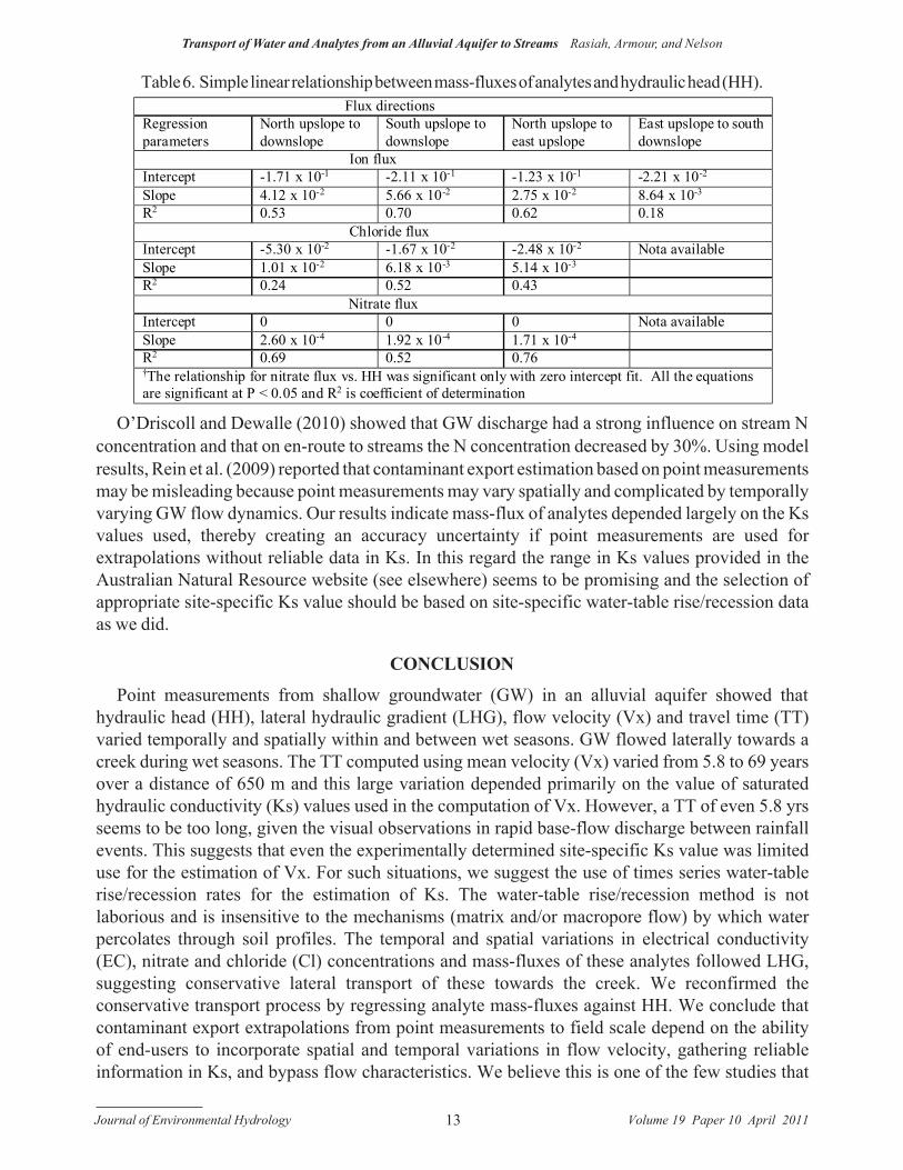
Coupling flux-theory and statistics to analyse the behaviour of analytes

Nitrate-N mass-flux from north upslope to downslope during the 2007 wet season varied from1.0 x 10-4 to 4.4 x 10-3 g m-2- d-1, Cl from 1.77 x 10-2 to 1.01 x 10-1 g m-2 d-1, and total solutes (EC)from 3.0 x 10-2 to 3.8 x 10-1 g m-2 d-1 (Figure 4). The variations along the southern transect segmentwere 1.0 x 10-2 to 2.24 x 10-1 g m-2 d-1 for nitrate, 7.14 x 10-3 to 4.95 x 10-2 g m-2 d-1 for Cl, and2.2 x 10-2 to 5.83 x 10-1 g m-2 d-1 for EC (Figure 5). The CVs indicate analyte concentrations variedduring and between wet seasons and in some cases the variations were larger than HH (Table 4).It is apparent from the values of CVs for analyte concentrations the temporal variation was highestfor nitrate, followed by Cl and EC. The time-series plots indicate there were close associationsbetween LHG and analyte fluxes (Figures 4 and 5). Because LHG was used in the computation ofanalyte fluxes we regressed the latter against HH and found that approximately 18 to 70% of ion(EC) fluxes were controlled by HH, compared with 24 to 52% for Cl, and 52 to 76% for nitrate(Table 6). It should be noted the linear fit of nitrate vs. HH was obtained for a zero intercept. Thereseems to be contradiction between the characterisation of temporal variations by CV and R2. Wehave discussed this aspect previously and suggested the CV’s reflect overall seasonal variation andR2 the influence of individual storm (CRF). Regardless of the differences in responses, theprimary driver responsible for the temporal variations in analytes was rainfall induced variationsin HH.

Chloride distribution/redistribution in unsaturated soil profiles has extensively been used assignature indicator to delineate subsurface flow pathways (Radford et al. 2009; Rasiah et al. 2005;O’Geen et al. 2002). The relatively high R2 for EC and Cl suggest that EC along with Cl can be usedas signature indicator or conservative tracer to track lateral flow of water and solutes in non-salinesaturated regolith in this wet tropical environment. Though the R2 for zero intercept for nitrate vs.HH linear fit was high there might have been nitrate attenuation by denitrification or dissimilatoryreduction to ammonium (Kellogg et al. 2005; Hanson and Hoffman, 1994). This implies thatnitrate export from GW to streams may be low, perhaps because the travel time required or theresidence time GW is relatively long compared with the rate of nitrate attenuation reductions. Theaforementioned long travel time is for export from upslope to the creek, but in reality the exportto creek was from downslope. The travel time from downslope to creek is approximately 1 monthfor Ks= 300 mm h-1 or approximately 1 yr for Ks= 25 mm hr-1, implying export risk is significant.The anion adsorption capacity of these alluvial soils is not known to suggest nitrate adsorption insoil matrix played any role in the fate of nitrate in GW. The negative intercepts for EC and Clsuggest potential reverse fluxes of analytes from the creek to GW and negative LHG obtained aftermid-June support this claim.



Figure 5. Time series plots showing the influence of lateral hydraulic gradient on conservative transport ofions (Figure 5a), chloride (Figure 5b), and nitrate (Figure 5c) form southern upslope to downslope and iontransport from northern upslope to east upslope (Figure 5d). Note the differences in units in both X and Yaxes.

Figure 4. Time series plots showing the influence of lateral hydraulic gradient on conservative transport ofions (Figure 4a), chloride (Figure 4b), and nitrate (Figure 4c) from northern upslope to downslope. Notethe differences in units in both X and Y axises.



O’Driscoll and Dewalle (2010) showed that GW discharge had a strong influence on stream Nconcentration and that on en-route to streams the N concentration decreased by 30%. Using modelresults, Rein et al. (2009) reported that contaminant export estimation based on point measurementsmay be misleading because point measurements may vary spatially and complicated by temporallyvarying GW flow dynamics. Our results indicate mass-flux of analytes depended largely on the Ksvalues used, thereby creating an accuracy uncertainty if point measurements are used forextrapolations without reliable data in Ks. In this regard the range in Ks values provided in theAustralian Natural Resource website (see elsewhere) seems to be promising and the selection ofappropriate site-specific Ks value should be based on site-specific water-table rise/recession dataas we did.

CONCLUSION

Point measurements from shallow groundwater (GW) in an alluvial aquifer showed thathydraulic head (HH), lateral hydraulic gradient (LHG), flow velocity (Vx) and travel time (TT)varied temporally and spatially within and between wet seasons. GW flowed laterally towards acreek during wet seasons. The TT computed using mean velocity (Vx) varied from 5.8 to 69 yearsover a distance of 650 m and this large variation depended primarily on the value of saturatedhydraulic conductivity (Ks) values used in the computation of Vx. However, a TT of even 5.8 yrsseems to be too long, given the visual observations in rapid base-flow discharge between rainfallevents. This suggests that even the experimentally determined site-specific Ks value was limiteduse for the estimation of Vx. For such situations, we suggest the use of times series water-tablerise/recession rates for the estimation of Ks. The water-table rise/recession method is notlaborious and is insensitive to the mechanisms (matrix and/or macropore flow) by which waterpercolates through soil profiles. The temporal and spatial variations in electrical conductivity(EC), nitrate and chloride (Cl) concentrations and mass-fluxes of these analytes followed LHG,suggesting conservative lateral transport of these towards the creek. We reconfirmed theconservative transport process by regressing analyte mass-fluxes against HH. We conclude thatcontaminant export extrapolations from point measurements to field scale depend on the abilityof end-users to incorporate spatial and temporal variations in flow velocity, gathering reliableinformation in Ks, and bypass flow characteristics. We believe this is one of the few studies that

Flux directions Regression parameters

North upslope to downslope

South upslope to downslope

North upslope to east upslope

East upslope to south downslope

Ion flux Intercept -1.71 x 10-1 -2.11 x 10-1 -1.23 x 10-1 -2.21 x 10-2 Slope 4.12 x 10-2 5.66 x 10-2 2.75 x 10-2 8.64 x 10-3 R2 0.53 0.70 0.62 0.18 Chloride flux Intercept -5.30 x 10-2 -1.67 x 10-2 -2.48 x 10-2 Nota available Slope 1.01 x 10-2 6.18 x 10-3 5.14 x 10-3 R2 0.24 0.52 0.43 Nitrate flux Intercept 0 0 0 Nota available Slope 2.60 x 10-4 1.92 x 10-4 1.71 x 10-4 R2 0.69 0.52 0.76 †The relationship for nitrate flux vs. HH was significant only with zero intercept fit. All the equations are significant at P < 0.05 and R2 is coefficient of determination

Table 6. Simple linear relationship between mass-fluxes of analytes and hydraulic head (HH).



have coupled flux-theory and statistics to identify the major variables that control contaminantexport from GW to surface-water.

ACKNOWLEDGMENTS

Dr. Chris Carroll (Principal Scientist) and Ms. Glynis Orr (Senior Hydrologist) at theDepartment of Environment and Resource Management, Queensland, Australia, reviewed thismanuscript. We extend our sincere thanks and gratefully acknowledge their contribution viacomments, suggestions, and editorial input. The financial support provided by the AustralianResearch Council, the field and laboratory support provided by Mr. D. H. Heiner, Ms. T. Whiteing,Mr. M. Dwyer, and Ms. D. E. Rowan are gratefully acknowledged.

REFERENCES

Alexander, D.G. 2000. Hydrographic procedure for water quality sampling. Water Monitoring Group, WaterResource Information & Systems Management. Department of Natural Resources, Brisbane, Australia.

Baker, J. 2003. A Report on the Study of Land-Sourced Pollutants and their Impacts on Water Quality in andAdjacent to the Great Barrier Reef. Department of Primary Industries, Brisbane. QLD, Australia.

Bell, M.J., B.J. Bridge, G.R. Harch, and D.N. Orange. 2005. Rapid internal drainage rates in Ferrosols. Aust. J.Soil Res., Vol. 43, pp. 443-455.

Bonell, M.D., A. Gilmour, and D.S. Cassell. 1983. A preliminary survey of the hydraulic properties of the rainforestsoils in the tropical North-East Queensland and their implications for the runoff process. Catena, Vol. 4, pp.57-78.

Brodie, J., L. McKergow, I.P. Prosser, M. Furnas, A.O. Hughes, and H. Hunter. 2003. Sources of Sediment andNutrient Exports to the Great Barrier Reef World Heritage Area. ACTFR Report 03/11. Townsville, Australia.

Cook, P.G., and N.I. Robinson. 2002. Estimating groundwater recharge in fractured rock from environmental 3Hand 36Cl, Clare Valley, South Australia. Water Res. Res, Vol. 35(2), pp.1136-1142.

Cook, P.G., A.L. Herczeg, and K.L. McEwan. 2001. Groundwater recharge and stream baseflow: AthertonTablelands, Queensland. CSIRO Land and Water. Technical Report 08/01, April 2001. Canberra, Australia.

Crosbie, R.S., J.L. McCallum, and G.A. Harrington. 2009. Estimation of groundwater recharge and dischargeacross northern Australia. 18th World IMACS/MODSIM Congress, Cairns, Australia 13-17th July 2009.(http://mssanz.org.au/modsim09)

De Vries, J.J., and I. Simmers. 2002 Groundwater recharge: an overview of processes and challenges.Hydrogeology Journal, Vol. 10(1), pp.5-17

Fetter, C.W. 1999. Contaminant Hydrogeology, 2nd ed., Prentice Hall, ISBN 0137512155.Gu, C., and R.J. Riley. 2009. Combined effects of short term rainfall patterns and soil texture on soil nitrogen

cycling – A modelling analysis. J. Contaminant Hydrology, Vol. 112, pp. 141-154.Hair, I.D. 1990. Hydrogeology of the Russell and Johnstone Rivers Alluvial valleys, North Queensland. ISBN

1034 7399, Department of Resource Industries, Brisbane, Australia.Hanson, G.C., and P.M. Hoffman. 1994. Denitrification rates in relation to groundwater level in a peat soil under

grassland. J. Environmental Quality, Vol. 23, pp. 917-922.Healy, R.W., and P.G. Cook. 2002. Using groundwater levels to estimate recharge. Hydrology Journal, Vol.10,

pp. 99-109Jolly, I.D. and D.W. Rassam. 2009. A review of modelling of groundwater-surface water interactions in arid/semi-

arid floodplains. 18th World IMACS / MODSIM Congress, Cairns, Australia 13-17 July 2009.http://mssanz.org.au/modsim09 .

Kalbus, E., C. Schmidt, M. Bayer-Raich, S. Leschik, F. Reinstorf, G.U. Blacke, and M. Schirmer. 2007. Newmethodology to investigate potential contaminant mass fluxes at the stream–aquifer interface by combiningintegral pumping tests and streambed temperatures. Environmental Pollution, Vol. 148, pp. 808-816.

Kellogg, D.Q., A.J. Gold, P.M. Groffman, K. Addy, M.H. Stolt, and G. Blazejewski. 2005. In-situ ground waterdenitrification in stratified, permeable soils underlying riparian wetlands. J. Environmental Quality, Vol. 34,



pp. 524-533.Larkin, R.G., and J.M. Sharp Jr. 1992. On the relationship between river-basin geomorphology, aquifer hydraulics,

and groundwater flow direction in alluvial aquifers. GSA Bulletin, Vol. 104, pp. 1608-1620.LaSage, D.M., A.E. Fryar, M.A. Mukherjee, N.C. Sturchio, and L.J. Heraty. 2008. Groundwater-derived

contaminant fluxes along a channelized Coastal Plain stream. J. Hydrology, Vol. 360, pp. 265-280.Moody, P.W., J.R. Reghenzani, J.D. Armour, B.G. Prove, and T.J. McShane. 1996. Nutrient balances and

transport at farm scale- Johnstone River Catchment. In: Hunter HM, Eyles GE, Rayment G. (Eds.),Downstream Effects of Land Use. Department of Natural Resources, Brisbane, Australia.

Ninghu Su., P.N. Nelson, and S. Connor. 2010. Determining aquifer hydraulic parameters using slug tests and thesolution of a fractional diffusion-wave equation. J. Hydrology (in review).

O’Geen, A.T., P.A. McDaniel, and J. Boll. 2002. Chloride distributions as indicators of vadose zone stratigraphyin Palouse loess deposits. Vadose Zone Journal, Vol. 1, pp. 150-157.

O’Driscoll, M.A., and D.R. Dewalle. 2010. Seep regulates stream nitrate concentration in a forested Appalachiancatchment. J. Environmental Quality, Vol. 39, pp. 420-431.

Praamsma, T., K.Novakowski, K. Kyser, and K. Hall. 2009. Using stable isotopes and hydraulic head data toinvestigate groundwater recharge and discharge in a fractured rock aquifer. J. Hydrology, Vol. 366, pp.35-45.

Radford, B.J., D.M. Silburn, and M. Forster. 2009. Soil chloride and deep drainage responses to land clearing forcropping at seven sites in central Queensland, northern Australia. J. Hydrology, Vol. 379, pp. 20-29.

Rasiah, V., J.D. Armour, A.L. Cogle, and S.K. Florentine. 2010. Nitrate import-export dynamics in groundwaterinteracting with surface-water in a wet-tropical environment. Aust. J. Soil Res., Vol. 48, pp. 361-370.

Rasiah, V., J.D. Armour, and A.L. Cogle. 2007. Statistical characterisation of impact of system variables ontemporal dynamics of groundwater in highly weathered regoliths. Hydrological Processes, Vol. 21, pp. 2435-2446.

Rasiah, V., J.D. Armour, and A.L. Cogle. 2005. Assessment of variables controlling nitrate dynamics ingroundwater: Is it a threat to surface aquatic ecosystems? Marine Pollution Bulletin, Vol. 51, pp. 60-69.

Rasiah, V., J.D. Armour, T. Yamamoto, S. Mahendrarajah, and D.H. Heiner. 2003. Nitrate dynamics in shallowgroundwater and the potential for transport to off-site water bodies. Water Air and Soil Pollution, Vol. 147,pp. 183-202.

Rasiah, V., G.C. Carlson, and R. A. Kohl. 1992. Assessment of functions and parameter estimation methods inroot water uptake simulation. Soil Sci. Soc. Am. J., Vol. 56, pp. 1267-1272.

Rayment, G.R., and F.R. Higginson. 1992. Australian Laboratory Handbook of Soil and Water Chemical Methods,Inkata Press, Sydney, Australia.

Rein, A., S. Bauer, P. Dietrich, and C. Beyer. 2009. Influence of temporally variable groundwater flow conditionson point measurements and contaminant mass flux estimations. J. Contaminant Hydrology, Vol. 108, pp. 118-133.

Russell, J.S., and R.F. Isbell. 1986. The Australian Soils: the Human Impact. St. Lucia, University of QueenslandPress. ISBN 0702219681.

Scanlon, B.R., R.P. Langford, and R.S. Goldsmith. 1999. Relationship between geomorphic settings andunsaturated flow in an arid setting. Water Res. Res., Vol. 35(4), pp. 983-999.

Statistical Analysis Systems. 1991. SAS/STAT Procedure Guide for Personal Computers, Version 5. StatisticalAnalysis Systems Institute Inc. Cary, NC.

von Asmuth, J.R., and M. Knotters. 2004. Characterising groundwater dynamics based on a system identificationapproach. J. Hydrology, Vol. 296, pp. 118-134.

ADDRESS FOR CORRESPONDENCEV. RasiahDepartment of Environment and Resource Management5B Sheridan StreetPO Box 937Cairns QLD 4870Australia

[email protected]

full paper - international association for environmental hydrology

Documents