full cycle cylinder state estimation in di engines with...

Master of Science Thesis in Electrical EngineeringDepartment of Electrical Engineering, Linköping University, 2019

Full Cycle Cylinder StateEstimation in DI Engineswith VVA

Linus Johansson

Master of Science Thesis in Electrical Engineering

Full Cycle Cylinder State Estimation in DI Engines with VVA

Linus Johansson

LiTH-ISY-EX--19/5221--SE

Supervisor: Max Johanssonisy, Linköping University

Erik HöckerdalScania CV AB

Examiner: Lars Erikssonisy, Linköping University

Division of Automatic ControlDepartment of Electrical Engineering

Linköping UniversitySE-581 83 Linköping, Sweden

Copyright © 2019 Linus Johansson

Sammanfattning

Högre ställda krav på emissioner kräver bättre förståelse för förloppen inomcylindern. Cylindermodellen som tagits fram inom exjobbet bidrar med attkunna använda samma uppsättning ekvationer för förloppen insug, kompression,expansion/förbränning och avgastakt. En cylindermodell med tillståndentemperatur, tryck och massfraktion luft har tagits fram.

Modellen hanterar gasväxling via variabla kompressibla flöden för ventiler därkamfasning, dekompressionsbroms och blowby hanteras. Föbränning modellerasmed en enkel Vibefunktion som beskriver värmefrigörelsen samt konsumptionav luft.

Modellen är gjord för att vara generell och kunna användas på såväl SI somCI motorer. De kalibreringar som behövs är strömmningsmotståndskoefficientCD för avgas, insugsventil och blowby samt parametrar för värmeöverföring/ frigörelse. Dessutom måste olika motorgeometriparametrar sättas för attkunna räkna ut den momentana cylindervolymen. Modellen har visat godöverensstämelse för cylindertryckkurvor med och utan förbränning därventilerna fasats olika mycket. Det visar att den kan hantera de viktiga fallen somförekommer i förbränningsmotorer. Det går med enkelhet att ersätta delmodelleri modellen t.ex. enkel Vibe mot dubbel Vibe. En utsignal är Φ i cylindern,dessutom räknas skattat indikerat medelmoment för hela motorn fram utifråntillstånden i en cylinder. Dessa två uträkningar har stämt väl överens medstationära mätningar utförda i motorprovcell. Modellen klarar av fix steglängdför jämn processorlast, steglängderna har varit tillräckligt långa för att modellenrimligen kan användas för realtidsimplementering på motorstyrenhet.

iii

Abstract

Tougher legal demands on pollutions require a better developed understandingof the processes that take place in the cylinder. The thesis contributes witha cylinder model that uses the same set of equations for intake, compression,expansion/combustion and exhaust. The cylinder model describes the statestemperature, pressure and the mass fraction of air.

The model is able to simulate the gas exchange with compressible flows over thevalves, it handles VVT, CRB and blowby. The combustion is modeled with asingle Vibe function that describes the heat release and the consumption of air.

The model is general enough to be able to simulate both SI and CI engines. Thecalibrations that are needed are the discharge coefficient CD values for intakeand exhaust valves, blowby, and heat release/transfer parameters. Furthermore,the engine geometry parameters have to be provided to be able to calculatethe instanteneous cylinder volume. The model has shown good agreement forcylinder pressure curves with and without combustion and can handle phasingof the valve lifts. That shows that the model can handle the important casesin combustion engines. It is easy to replace sub models in the cylinder modele.g. single Vibe with double Vibe. In the model, Φ in the cylinder is calculatedand the average instantenous torque for the entire engine is calculated from thestates in one cylinder. These two calculations have shown good agreement withthe stationary measurments done in an engine test cell. The model is able touse fixed step lengths for even processor loads, the size of the step lengths areresonable for real time implementation on an ECU.

v

Acknowledgments

I would like to show my gratitude to my family and especially my girlfriendMatilda for always believing in me and for all support during the past years.I would like to thank all friends I have made during my studies in Linköping.Without you I would not have come this far. I would like to thank Scania CV ABfor the opportunity of writing this thesis and especially my supervisor at ScaniaErik Höckerdal for all the guidance and for always having time for discussion.I would also like to thank all my collegues at NCPP for the coffee breaks andinteresting discussions. I would also like to show my gratitude to my examinerLars Eriksson for introducing me to the exciting world of automotive engineeringand finally a big thank you to my supervisor at ISY Max Johansson.

Södertälje, June 2019Linus Johansson

vii

Contents

Notation xi

1 Introduction 11.1 Objectives . . . . . . . . . . . . . . . . . . . . . . . . . . . . . . . . 11.2 Delimitations . . . . . . . . . . . . . . . . . . . . . . . . . . . . . . . 11.3 Related Work . . . . . . . . . . . . . . . . . . . . . . . . . . . . . . . 21.4 Thesis Outline . . . . . . . . . . . . . . . . . . . . . . . . . . . . . . 2

2 Theory 52.1 The Four Stroke Cycle in a CI-Engine . . . . . . . . . . . . . . . . . 52.2 Engine Geometry . . . . . . . . . . . . . . . . . . . . . . . . . . . . 62.3 Ideal Gas . . . . . . . . . . . . . . . . . . . . . . . . . . . . . . . . . 82.4 Thermodynamic States . . . . . . . . . . . . . . . . . . . . . . . . . 82.5 Gas Properties . . . . . . . . . . . . . . . . . . . . . . . . . . . . . . 11

2.5.1 Air . . . . . . . . . . . . . . . . . . . . . . . . . . . . . . . . 112.5.2 Gas Relations . . . . . . . . . . . . . . . . . . . . . . . . . . 112.5.3 NASA Polynomials . . . . . . . . . . . . . . . . . . . . . . . 132.5.4 Gatowski’s Model . . . . . . . . . . . . . . . . . . . . . . . . 14

2.6 Gas Exchange . . . . . . . . . . . . . . . . . . . . . . . . . . . . . . 142.6.1 Compressible Flow . . . . . . . . . . . . . . . . . . . . . . . 152.6.2 VVA . . . . . . . . . . . . . . . . . . . . . . . . . . . . . . . . 172.6.3 CRB . . . . . . . . . . . . . . . . . . . . . . . . . . . . . . . . 172.6.4 Blowby . . . . . . . . . . . . . . . . . . . . . . . . . . . . . . 17

2.7 Heat Transfer . . . . . . . . . . . . . . . . . . . . . . . . . . . . . . . 172.8 Combustion . . . . . . . . . . . . . . . . . . . . . . . . . . . . . . . 18

2.8.1 Ignition Delay . . . . . . . . . . . . . . . . . . . . . . . . . . 182.9 Combustion Modelling . . . . . . . . . . . . . . . . . . . . . . . . . 192.10 Heat Release Analysis . . . . . . . . . . . . . . . . . . . . . . . . . . 20

2.10.1 Net Heat Release Analysis . . . . . . . . . . . . . . . . . . . 202.10.2 Rassweiler and Withrow’s Method . . . . . . . . . . . . . . 21

2.11 Mass Fraction Burned . . . . . . . . . . . . . . . . . . . . . . . . . . 222.11.1 Matekunas Pressure Ratio . . . . . . . . . . . . . . . . . . . 222.11.2 Polytrope . . . . . . . . . . . . . . . . . . . . . . . . . . . . . 22

ix

x Contents

2.12 Analytic Pressure Model . . . . . . . . . . . . . . . . . . . . . . . . 23

3 Modelling 253.1 Gas Flows . . . . . . . . . . . . . . . . . . . . . . . . . . . . . . . . . 25

3.1.1 Oscillating Mass Flow . . . . . . . . . . . . . . . . . . . . . 263.1.2 Blowby Flow . . . . . . . . . . . . . . . . . . . . . . . . . . . 28

3.2 Gas Properties . . . . . . . . . . . . . . . . . . . . . . . . . . . . . . 283.2.1 Combustion Gas Properties . . . . . . . . . . . . . . . . . . 29

3.3 Heat Transfer . . . . . . . . . . . . . . . . . . . . . . . . . . . . . . . 313.3.1 Woschni . . . . . . . . . . . . . . . . . . . . . . . . . . . . . 31

3.4 Torque Model . . . . . . . . . . . . . . . . . . . . . . . . . . . . . . 32

4 Data acquisition 354.1 Absolute Reference Of Cylinder Pressure . . . . . . . . . . . . . . . 37

5 Result and Discussion 395.1 Motored Pressure . . . . . . . . . . . . . . . . . . . . . . . . . . . . 405.2 CRB . . . . . . . . . . . . . . . . . . . . . . . . . . . . . . . . . . . . 445.3 Combustion . . . . . . . . . . . . . . . . . . . . . . . . . . . . . . . 475.4 Real Time Feasibility Study . . . . . . . . . . . . . . . . . . . . . . . 54

6 Future Work 55

A Model Parameters 59A.1 Gas Properties . . . . . . . . . . . . . . . . . . . . . . . . . . . . . . 59A.2 Valve Properties . . . . . . . . . . . . . . . . . . . . . . . . . . . . . 60

Bibliography 63

xii Notation

Notation

Abbreviations

Abbreviation Description

AMB AmbientBDC Bottom Dead CenterCA Crank Angle

CHEPP Chemical Equilibrium Program PackageCI Compression IgnitedCN Cetane NumberCRB Compression Release BrakeDI Direct InjectedDS Downstream

ECU Engine Control UnitEGR Exhaust Gas RecirculationEVC Exhaust Valve ClosingEVO Exhaust Valve OpeningHIL Hardware in the LoopHLA Hydraulic Lash AdjustersHT Heat TransferHR Heat ReleaseICE Internal Combustion EngineIVC Intake Valve ClosingIVO Intake Valve OpeningMFB Mass Fraction Burned

MVEM Mean Value Engine ModelsSI Spark Ignited

SOC Start Of CombustionSOI Start Of InjectionTDC Top Dead CenterUS Upstream

VVA Variable Valve ActuationVVT Variable Valve Timing

Notation xiii

Constants

Constant Description

AR Reference Area [m2](A/F)s Stoichiometric Air/Fuel Ratio [-](F/A)s Stoichiometric Fuel/Air Ratio [-]ncyl Number Of Cylinders [-]M Molar Mass [g/mole]pamb Ambient Pressure [Pa]Tamb Ambient Temperature [K]QLHV Lower Heating Value [MJ/kg]

R = 8.3143 Gas Constant [J/(mol K)]

Variables

Variable Description

AE Effective Area [m2]CD Discharge Coefficient [-]cv Specfic Heat At Constant Volume [J / (mole K)]cv Mass Specfic Heat At Constant Volume [J / (kg K)]cp Specfic Heat At Constant Pressure [J / (mole K)]cp Mass Specfic Heat At Constant Pressure [J / (kg K)]Dv Valve Head Diameter [mm]EA Activation Energy [J/mole]Lv Valve Lift [mm]Me Engine Torque [Nm]mf Mass Fuel Injected [kg]n Number of Moles [mole]Ne Engine Speed [rpm]pm Motored Pressure [Pa]p Pressure [Pa]Q Heat [W]T Temperature [K]V Volume [m3]Sp Mean Piston Speed [m/s]xb MFB [-]x Mass fraction [-]x Mole fraction [-]ηco Combustion Efficiency [-]

γ =cpcv

Specific Heat Ratio [-]κ Polytropic Exponent [-]τid Ignition Delay [CA]ωe Engine Speed [rad/s]λ Air Fuel Ratio [-]Φ Fuel Air Ratio [-]

1Introduction

In the coming years the legislation will be tougher on pollution from vehicles. InÅkerman (2019) it is described that the EU parliament have decided that the CO2emissions for new trucks will have to decrease by 30% from the levels emittedin 2019 until 2030. To achieve this a further understanding of the physicalphenomena that take place inside the cylinder is vital. Therefore a model thatcan estimate the state of the cylinder is needed. The understanding of the processin the cylinder gives tools to improve the fuel economy. That is of great interestsince the fuel is a major part of the cost of maintaining a truck. The contributionof this thesis is to use the same model structure for all the different phases in thefull four stroke cycle. Previous work has mostly been either on the open cyclewhere there is gas exchange or on the closed cycle when the valves are closed.

1.1 Objectives

The objective of this thesis is to model the cylinder pressure trace and otherthermodynamic states over the full cycle in a CI engine. The goal is that themodel will handle special cases like cam phasing, Variable Valve Timining (VVT)and how it affects the gas exchange. The model will also have a combustion andheat transfer model and include contributions from blowby. The model will beas generic as possible so that the structure with small modifications can be usedwhen simulating cylinder states in SI engines.

1.2 Delimitations

Items that are outside the scope of this thesis are:

1

2 1 Introduction

• Multi-zone combustion models

• EGR

• Fuel spray models

• Crevice effects

• Thermal stress and solid mechanics that affects cylinder volumecalculations.

• Warm up process of the engine.

• Formation of emissions.

• Data collection on different engines.

• Implementation of a control system.

1.3 Related Work

Previous work on cylinder pressure have most often used the cylinder pressurefor studying the heat release. That has been done in several works for exampleGatowski et al. (1984), Klein (2007) and Egnell (2000). In those works the heattransfer most often uses the empirical observation made by Woschni (1967).Modeling the cylinder pressure have been made in Eriksson and Andersson(2002). There, an analytical cylinder pressure model was developed for an SI-engine. That model did not rely on solving differential equations in each step.However that model does not take heat transfer directly into account or the effectthat the gas properties changes when there is internal EGR (residual gases) andchange in temperature. The model needs to be fitted to many different cases.Templin (2002) used a crank angle based cylinder pressure model for modelingcompression release brake (CRB). In the article it was argued that CRB takesplace during one cycle and therefore needs a crank based pressure model. Theintention of this thesis is to also model CRB in the same framework.

The combustion is most often modelled by Vibe functions presented in Vibe andMeißner (1970). The idea in this thesis is to use a single Vibe function to makea simple combustion model. The Vibe function is parameterized by studying theheat release. The heat release can be obtained from the cylinder pressure databy methods described by Krieger and Borman (1966), Rassweiler and Withrow(1938) and Sellnau et al. (2000). Klein (2007) mentions that Matekunas pressureratio concept has been shown to be able to predict MFB50 accurately.

1.4 Thesis Outline

In Chapter 1 the motivation of the thesis is presented and the work is put inrelation to previous work. Chapter 2 will describe the necessary theory to modelthe cylinder pressure. Chapter 3 will provide a description on how the model

1.4 Thesis Outline 3

is implemented and the different algorithms used to estimate parameters. InChapter 4 the data collection and the limitations of some sensors are discussed.In Chapter 5 the results will be presented and discussed and finally in Chapter 6future work will be discussed.

2Theory

In this chapter the relevant theory needed when modeling the thermodynamiccylinder states for a four stroke CI engine is presented. Much of the theorypresented in this chapter is also applicable for SI engines.

2.1 The Four Stroke Cycle in a CI-Engine

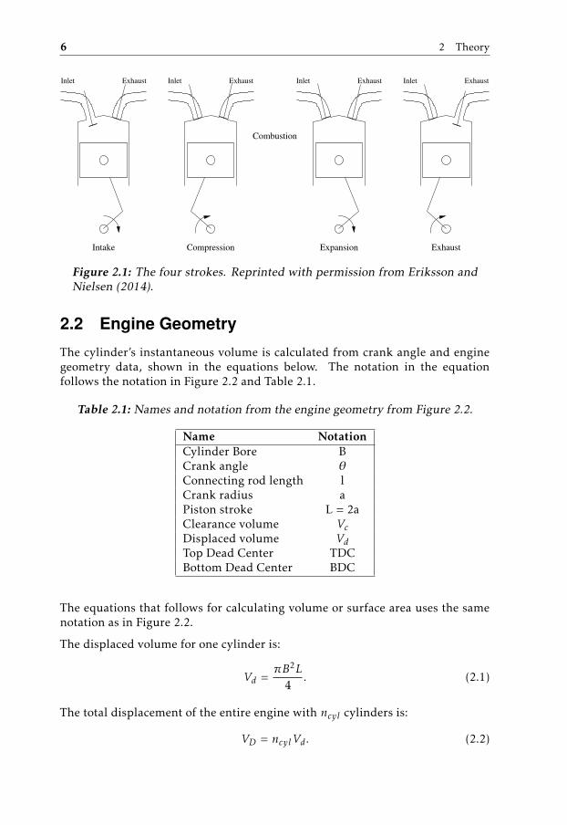
The four strokes in a CI-engine is explained below and is visualised in Figure 2.1.

1. Intake This is when the intake valve is opened and the cylinder is filledwith air. During the intake the cylinder pressure is close to the pressure inthe intake manifold. The piston moves from TDC to BDC.

2. Compression The valves are closed and the air is compressed to a higherpressure and temperature when the piston moves towards TDC. Fuel isinjected towards the end of the compression stroke. Combustion startswhen the fuel in the charge have diffused sufficiently with the air. Thecombustion continues through the power stroke.

3. Power stroke Work is performed by the fluid during the power stroke whenthe volume increases. When the exhaust valve is opened the blowdownstarts. The cylinder pressure decreases as the fluid is blown out to theexhaust system.

4. Exhaust The fluid is pushed out to the exhaust when the piston movestoward TDC again. The cylinder pressure is close to the pressure in theexhaust manifold. After this process the cycle is complete and it starts overwith the intake.

5

6 2 Theory

CompressionIntake Expansion Exhaust

Inlet Inlet Inlet InletExhaust Exhaust Exhaust Exhaust

Combustion

Figure 2.1: The four strokes. Reprinted with permission from Eriksson andNielsen (2014).

2.2 Engine Geometry

The cylinder’s instantaneous volume is calculated from crank angle and enginegeometry data, shown in the equations below. The notation in the equationfollows the notation in Figure 2.2 and Table 2.1.

Table 2.1: Names and notation from the engine geometry from Figure 2.2.

Name NotationCylinder Bore BCrank angle θConnecting rod length lCrank radius aPiston stroke L = 2aClearance volume VcDisplaced volume VdTop Dead Center TDCBottom Dead Center BDC

The equations that follows for calculating volume or surface area uses the samenotation as in Figure 2.2.

The displaced volume for one cylinder is:

Vd =πB2L

4. (2.1)

The total displacement of the entire engine with ncyl cylinders is:

VD = ncylVd . (2.2)

2.2 Engine Geometry 7

Engine – Introduction 73

4.2 Engine Geometry

BTDC

BDC

Vc

s(✓)

l

L

a

✓

Figure 4.3 Definitions of thecrankshaft, connecting rod,and cylinder geometries for anengine.

The geometry of the piston, connecting rod and crank isillustrated in Figure 4.3. The parameters shown in the figure andsome important derived parameters are:

Cylinder bore BConnecting rod length lCrank radius aPiston stroke L = 2aCrank angle ✓Clearance (minimum) volume Vc

Displaced volume Vd = ⇡ B2 L4

The displacement volume, Vd, is the volume that the pistondisplaces in the cylinder and the definition here gives the volumefor one cylinder. However Vd is often used to denote the totaldisplacement of the engine, i.e. VD = ncyl

⇡ B2 L4 (where ncyl is

the number of cylinders in the engine). Here VD = Vd ncyl will beused to denote the engine displacement.

The compression ratio, rc, is an important parameter thatinfluences the engine efficiency:

rc =maximum cylinder volumeminimum cylinder volume

=Vd + Vc

Vc

For spark ignited (SI) engines (also referred to as gasoline engines) the compression ratiousually lies in the range rc 2 [8, 12]. For diesel engines the compression ratio usually lies inthe range rc 2 [12, 24].

The instantaneous volume for the cylinder at crank position ✓ is given by

V (✓) = Vc +⇡B2

4(l + a � s(✓))

where s(✓) is the distance between the crank axis and the piston pin

s(✓) = a cos ✓ +p

l2 � a2 sin2 ✓

In the expressions above the volume is specified in terms of the geometric parameters but theexpressions are complex and hide some structure. It is possible to rewrite the expressions to

V (✓) = Vd

24 1

rc � 1+

1

2

0@ l

a+ 1 � cos ✓ �

s✓l

a

◆2

� sin2 ✓

1A35 (4.3)

and from this expression we see how the displacement volume Vd, the compression ratio rc,and the l

a -ratio influence the cylinder volume.

Figure 2.2: The engine geometry. Reprinted with permission from Erikssonand Nielsen (2014).

The compression ratio can be calculated with:

rc =maximum cylinder volumeminimum cylinder volume

=Vd + VcVc

(2.3)

The instanteneous volume of one cylinder as an expression of the crank angle θ:

V (θ) = Vd

1rc − 1

+12

la + 1 − cos(θ) −

√(la

)2

− sin2(θ)

(2.4)

The derivative of equation (2.4) is:

dV (θ)dθ

=12Vd sin(θ)

1 +cos(θ)√(

la

)2− sin2(θ)

(2.5)

Equation (2.5) can be calculated in the time domain with usage of the chain rule

dV (θ)dt

=dV (θ)dθ

dθdt︸︷︷︸ωe

=dV (θ)dθ

ωe. (2.6)

8 2 Theory

The area of the combustion chamber, piston crown and cylinder head dependingon θ:

A(θ) = (l + a − s(θ))πB +2πB2

4(2.7)

s(θ) = a cos(θ) +√l2 − a2 sin2(θ) (2.8)

The area is of interest when calculating the heat transfer. There is howeversimplifications on calculating the instantaneous volume based on enginegeometry. During the engine operation the components around the combustionchamber are exposed to thermal forces and pressure forces. These forces willdeform the components which will make the volume deviate from the ideal. InAnagrius West et al. (2018) it was concluded that the instantaneous volume candeviate as much as 6% from the geometrical at TDC. That study was conductedon an inline six cylinder Scania engine.

2.3 Ideal Gas

An equation of states is an equation that relates pressure p, temperature T andvolume V as

f (p, T , V ) = 0 (2.9)

The most common equation of states is the ideal gas law

pV = nRT = mRMT = mRT (2.10)

The ideal gas law can either be expressed in moles or with mass. R in the equationdepends on what type of gas it is while R is a constant.

It has been shown experimentally that real gases obey the ideal gas law at lowdensities. Many gases behave as ideal gases in intervals used in engineeringapplications and the ideal gas assumption can be made with small errors. Thereare other equations of state for example Van der Waals equation which is moreaccurate than the ideal gas law for real gases. At small densities Van der Waalsequation reduces to the ideal gas law. However these equations of states cannothandle transition from gas to liquid (Cengel et al., 2017).

Heywood (2019) concludes that the gas species that makes up the working fluidin ICE usally can be treated as ideal gases.

2.4 Thermodynamic States

The first law of thermodynamics describes the rate of change for the internalenergy see eqution (2.11). H describes the enthalpy flow, Q describes the heatrelase and heat transfer. W describes the mechanical power from p dVdt .

2.4 Thermodynamic States 9

Figure 2.3: The flows in and out of the cylinder.

In Figure 2.3 the flows in to the cylinder are shown. The flows are taken aspostitive if they flow as in the Figure while they are negative if they flow in theopposite direction.

The first law of thermodynamics for the system in Figure 2.3 is

dUdt

=∑i

Hi − Q − W (2.11)

In equation (2.11) i denotes the different flows to and from the cylinder. Theflows are defined as in Figure 2.3.

The enthalpy flow is described by the following relation

H = mcpT (2.12)

In the single zone model the enthalpy flow will be replaced with the specificenthalpy and massflows.

H = hm (2.13)

Considering thermodynamic relations the internal energy can be expressed asthe following:

U = mcvdT (2.14)

10 2 Theory

By differentiating the internal energy an expression for the temperaturediffrential can be obtained see equation (2.15).

dUdt

=d(mu)dt

=∑i

u(T )dmidt

+ mdudt

Eq: (2.14)︷︸︸︷=

∑i

u(T )dmidt

+ mcvdTdt

(2.15)

By inserting equation (2.15) into (2.11) equation (2.16) is obtained.

mcvdTdt

=∑i

(h′i − u)dmidt− dQdt− dWdt

dTdt

=RTpV cv

∑i

(h′i − u)dmidt− dQdt− pdV

dt

(2.16)

In the last step the ideal gas law have been used to remove m from the equation.u is the internal energy of the cylinder, h′ is the mass specific enthalpy and it isevaluated from where the flow origins (Heywood, 2019).

To get an expression for the pressure the ideal gas law in equation (2.10) isdiffrentiated.

Vdp

dt+ p

dVdt

= RT∑i

dmidt

+ mRdTdt

dp

dt=RTV

∑i

dmidt−p

VdVdt

+p

TdTdt

(2.17)

Thereby temperature and pressure is selected as the two states according toequation (2.18).

dTdt

dpdt

=

RTpV cv

(∑i

(h′i − u) dmidt −dQdt − p

dVdt

)RTV

∑i

dmidt −

pVdVdt + p

TdTdt

(2.18)

In the derivation of the thermodynamic states crevice effects have been neglectedsince the engine is Direct Injected (DI). In DI engines the fuel is injected intoa cavity in the piston and it is thereby kept from entering crevices (Johansson,2017). Crevices are regions where fuel can enter and avoid combustion. Inport injected engines crevice effects has to be considered since the air and fuel ispremixed and the flame does not reach the fuel in the crevices (Heywood, 2019).Other assumptions made in this derivation is that the temperature is homogenousin the entire cylinder.

2.5 Gas Properties 11

The ideal gas can be used to calculate the mass that is trapped in the cylinder as

m =pV

RT(2.19)

2.5 Gas Properties

The gas composition in the cylinder is considered to be a pure substance. A puresubstance means that the gas composition is homogenous. A commonly usedassumption for ICE is that the working fluid is air. It is called the air-standardassumtion (Cengel et al., 2017). The assumption is as follows:

1. The working fluid is air, which is circulated in a closed loop and alwaysbehaves as an ideal gas.

2. All processes that make up the cycle are internally reversible.

3. The combustion process is replaced by an external heat addition.

4. The exhaust process is replaced by a heat rejection process that restores theworking fluid to its initial state.

2.5.1 Air

Air is a mixture of many gases and the most vital element for combustion isoxygen. Oxygen is essential for engines since it oxidizes the fuel and it is theoxidation process that releases energy. The other gases are inert gases andhave minor effects on the combustion but they take up heat and space in thecombustion chamber. A commonly used model for air is discussed in Erikssonand Nielsen (2014) and it is to assume that air only consist of oxygen and nitrogen.Neglecting the other molecules present in air will lead to a small error, howeverthis error can be reduced if the other gases are lumped into nitrogen. Theconsideration that all molecules are nitrogen except oxygen gives that there are3.773 nitrogen molecules for each oxygen molecule. This leads to the followingmodel for air:

Air = O2 + 3.773N2 (2.20)

2.5.2 Gas Relations

In thermodynamical systems the specific heat ratio is often used, it is defined as

γ =cpcv. (2.21)

Assuming that a gas is ideal, gives the following relation between mass specificheats and the mass specific gas constant R = cp − cv .

The mole fraction x for specie i is defined as

x =nin

(2.22)

12 2 Theory

n is the total amount of moles of all species in the entire gas and ni is the amountof moles of specie i.

The mass fraction x for specie i is defined as

xi =mimtot

(2.23)

mi is the mass of specie i and mtot is the total mass.

For a gas consisting of several molecules where the mole/mass fraction xi/xi isknown the cp/cp value for the gas can be obtained by the following:

cp =∑i

xi cp,i (2.24a)

cp =∑i

xicp,i (2.24b)

The relation from mole fraction to mass fraction is the following

xi =mim

=xiMi∑j xjMj

(2.25)

The relation from mass fraction to mole fraction is the following

xi =nin

=xi /Mi∑jxj /Mj

(2.26)

The molecular weight of a gas containing different chemical species is needed tobe able to get the thermodynamic properties on a mass basis. In the equationbelow Mi is the molar mass of substance i, ni is how many moles there areof substance i and finally n denotes the total amount of moles of the differentmixtures in the gas.

M =1n

∑i

niMi =∑i

xiMi (2.27)

The scaling from molar basis to mass basis is the following

n =mM

(2.28)

m = nM (2.29)

Thereby all thermodynamic properties can be obtained in either molar basis orin mass basis and then be converted to the other.


R =RM

(2.30)

Given the ideal gas assumption cp and cv can be expressed in R and γ accordingto

cv =R

γ − 1(2.31)

cp =Rγ

γ − 1. (2.32)

The air/fuel equivalence ratio λ has the following definition

λ =mair

mf uel(A/F)s(2.33)

(A/F)s is the stochiometric air/fuel ratio. It tells the relation between the amountof air and fuel to have stochiometric reaction which between hydrocarbons andair only produces H2O and CO2. When there is excess air in the combustion, i.e.λ > 1, the mixture is said to be lean. If λ < 1 and there is excess fuel the mixtureis said to be rich.

It is also common to use Φ which is λ−1.

Φ = λ−1 =mf uel

mair (F/A)s(2.34)

The benefit of using Φ instead of λ is that Φ can handle when mf uel = 0. In the Φ

model a saturation is that Φ has its lowest value as 0.01 which means that λ = 100for cases with absense of combustion.

2.5.3 NASA Polynomials

The specific heat ratio will depend on temperature and a common way to modelthat is to use NASA polynomials. NASA polynomials is a database wherepolynomials have been fitted for different chemical species. The equations forthe NASA polynomials look like equation (2.35) where the coefficients variesdepending on which chemical specie it is (J. McBride et al., 2002).

cp(T )

R= a1 + a2T + a3T

2 + a4T3 + a5T

4 (2.35)

The NASA polynomials are specified for the common chemical species intemperature ranges 300-1000 K and 1000-5000 K. The coefficients in the NASApolynomials are different in those temperature ranges and are different forvarious chemical species. To obtain the cp for the whole gas equation (2.24a)is used.

14 2 Theory

Figure 2.4: γ for air dependent on temperature.

There is however other thermochemical programs that can be used to modelhow the gas properties varies with temperature and what chemical elements arepresent in the gas. One example of such a program is CHEPP. It is a chemicalequilibrium package designed for Matlab (Eriksson, 2005). It can calculatethermochemical properties for molecules and for combustion products. CHEPPwill in this work be used to benchmark the NASA polynomials and see that theimplementation is correctly made. In Figure 2.4 a comparison between CHEPPand NASA polynomials for air is shown. The NASA polynomials have used thesimplified model of air according to equation (2.20).

2.5.4 Gatowski’s Model

A commonly used model for γ is based on equation (2.36). That model wasorignally presented in Gatowski et al. (1984). It has been concluded in Kleinand Eriksson (2004) that equation (2.36) is difficult to get precise.

γ(T ) = γ300 + b(T − 300) (2.36)

In Eriksson and Nielsen (2014) it is stated that appropriate values for theconstants in equation (2.36) is γ300 ≈ 1.35 and that b ≈ 7 · 10−5.

To be able to parameterize equation (2.36) CHEPP could be used (Eriksson, 2005).

2.6 Gas Exchange

The gas exchange is the breathing of the engine. It is controlled by the camshaftwith the camlobes that pushes down the rocker arms which in turn push the

2.6 Gas Exchange 15

valves. The engine studied in this thesis can change when the camlobes will pushdown then rocker arms and the valves. It can also add a valve lift for compressionrelease brake (CRB).

2.6.1 Compressible Flow

The flow through poppet valves is often modeled as a compressible flow. This isneeded since the gas velocity is high. Components that has small cross sectionarea and large pressure difference are well described by isentropic compressibleflow (Eriksson and Nielsen, 2014). For a detailed derivation of compressible flowsee (Heywood, 2019, appendix C).

The flow is related to real gas flow effects by experimentally determineddischarge coefficients CD . CD for the intake and exhaust valves have beenmeasured in an airflow bench. The definition of CD is the following:

CD =actual mass flowideal mass flow

(2.37)

The CD values and the value of the reference area AR are linked together, theirproduct is the effective area AE .

AE = CDAR (2.38)

The isentropic compressible flow is described by equation (2.39).

m =pus√RTus

AEΨ li

(pdspus

)(2.39)

The index us abbreviation for upstream and means from were the flow originsand ds is an abbreviation for downstream and means where the flow ends. Figure2.5 shows that γ has negligible impact on the flow function and thereby it iscommon to use the assumption that γ is a constant.

16 2 Theory

Figure 2.5: The Ψ function for different γ values.

Equation (2.40) determines if the flow is choked or not. By choked flow it ismeant that the pressure reaches the critical sonic velocity.

Π

(pdspus

)= max

pdspus,

(2

γ + 1

) γγ−1

(2.40)

Ψ0(Π) =

√2γγ − 1

(Π

2γ −Π

γ+1γ

)(2.41)

Note when the pressure ratio between pdspus

is close to 1 the model does not fullfillthe Lipschitz condition. To be able to fullfill the Lipschitz condition a linearregion can be added.

Ψ li(Π) =

Ψ0(Π) if Π ≤ Πli

Ψ0(Πli)1−Π

1−ΠliOtherwise

(2.42)

The size of the linear region is difficult to determine beforehand. However inEllman and Piché (1999) a method of determining the size of the linear regionis presented. An indication to either add a linear region or to increase it is ifthere are oscillations present in the simulated mass flow of a component thatoperates at steady state (Eriksson and Nielsen, 2014). Equation (2.42) can beused to linearize the compressible flow equation. The boundary value when thelinear model is used or not is the tuning constant that needs to be investigated.

2.7 Heat Transfer 17

2.6.2 VVA

The valve event can be altered in any combination of the following (Dresner andBarkan, 1989).

1. Change the advance of valve event, while maintaining the same durationand lift profile.

2. Change valve event duration, while leaving the phase constant.

3. Modify lift characteristic, while leaving phase and duration constant.

4. Retain fixed valve timing and eliminate valve lift completely on selectedengine cylinders to vary the effective engine displacement.

The prototype engine used in this thesis can change the phase of the valve eventbut cannot alter duration. The engine can alter the lift profile by turning on/offthe CRB lift profile. There are several benefits in using VVT. It extends theuseful engine speed range. VVT can reduce emissions by the improvement inefficiency, because it will require less fuel. For some engines VVT can reduceemissions by controlling the internal EGR. Increasing the internal EGR reducesthe combustion temperature and thereby the amount of produced NOx.

2.6.3 CRB

Simply explained CRB turns the CI-engine into an air compressor. Rather than tostore the energy of the pressurised air created when the piston is coming up in thecompression stroke, the CRB hydraulically opens the exhaust valve near the endof the upward piston stroke. The stored energy in the cylinder is thus releasedto the exhaust manifold so when the piston enters the power stroke no pressureremains in the cylinder to act on the piston. The release of the compressed gasdissipates energy and the down movement in the expansion stroke is performedunder low pressure which leads to braking torque on the crankshaft (Cummins,1985). Note that CRB is often called Jacobs brake or Jake brake.

2.6.4 Blowby

Blowby is defined as the gas that flows from the combustion chamber into thecrankcase. The flow is mainly through the ring gaps. In a well maintained enginethe blowby flow accounts for about 1% of the total flow. The gases that ends upin the crankcase are ventilated back to the intake which will affect the propertiesin the intake systems. Earlier the gases that ended up in the crankcase wereventilated directly to the atmosphere and accounted for a significant source ofHC emissons (Heywood, 2019).

2.7 Heat Transfer

Heat transfer can occur due to convection, conduction and radiation. In enginesthe main heat transfer is from convection. Convection is the mode of heat transfer

18 2 Theory

between a solid surface and the adjacent liquid or gas that is in motion (Cengelet al., 2017). In CI engines there is also a contribution in the heat transfer fromradiation (Eriksson and Nielsen, 2014), which has been neglected in this thesis.Radiation is that energy is emitted by electromagnetic waves or photons as aresult of change in the electrons configuration (Cengel et al., 2017). The heattransfer due to convection from gas to cylinder wall is calculated using Newton’slaw of cooling:

QHT = hA∆T = hA(T − Tw) (2.43)

h is the convection heat transfer coefficient and is not a property of the fluid. It isan experimentally determined parameter whose value depends on all parametersinfluencing convection.

2.8 Combustion

The combustion in CI engines starts when the injected fuel ignites. It ischaracterized by three phases; ignition delay, premixed combustion and mixingcontrolled combustion.

2.8.1 Ignition Delay

Before the actual combustion starts in CI engines the fuel is transformed from acold liquid to a vapor and reach a sufficient temperature to autoignite. The timeit takes from SOI (start of injection) until the fuel autoignites is the ignition delay.This delay is not present in SI engines since the combustion starts when the fuelis ignited by a spark from the spark plugs.

There have been attempts to use experimental correlations to determine theigntion delay in CI engines. Traditionally Arrhenius correlations have been used,where A and n are tuning constants and EA is the activation energy for thereaction:

τid = Ap−nexp( EART

)(2.44)

Heywood (2019) suggests that the Arrhenius correlations does not seem usefulaccording to several reasons, one is that it is a to simple expression to representthe overall complex chemistry involved.

Another empirical formula developed by Hardenberg and Hase (1979) forpredicting the ignition delay in CI-engines has shown resonable agreement withexperimental data from different engine conditions (Heywood, 2019) :

τid(CA) = (0.36 + 0.22Sp)exp

EA ( 1RT− 1

17.190

)+

(21.2

p − 12.4

)0.63 (2.45)

2.9 Combustion Modelling 19

the cylinder pressure p in this equation is given in [bar].

The apparent activation energy EA is given by

EA =618.840CN + 25

(2.46)

where CN is the fuel cetane number. The cetane number is a measure on thefuels ability to resist autoignition (Heywood, 2019).

2.9 Combustion Modelling

The combustion has in this thesis used a single s-shaped Vibe function accordingto equation (2.47).

xb(θ) =

0, θ < θSOC

1 − e−a

(θ−θSOC

∆θ

)m+1

, θ ≥ θSOC(2.47)

In the Vibe functions ∆θ and a are related to the combustion duration and maffects the shape of the Vibe, θSOC denotes the start of combustion. The Vibefunction starts at 0 and goes to 1.

The derivative of the Vibe function with respect to θ is:

dxb(θ)dθ

=a(m + 1)

∆θ

(θ − θsoc∆θ

)me−a

(θ−θSOC

∆θ

)m+1

(2.48)

The combustion duration used in the Vibe function used the following ruleof thumb ∆θ = ∆θd + ∆θb (Eriksson and Nielsen, 2014). The parameter mhas been assigned a value and θSOC is taken when the MFB trace reaches asmall value. The parameter a has been optimized from MFB trace with theparameters discussed above used in the Vibe function. The optimization havebeen performed with lsqcurvefit in Matlab.

minx||F(x) − y||22 = min

x

∑i

(F(xi) − yi)2 (2.49)

lsqcurvefit solves nonlinear curve-fitting problem in a least-squares senseas described in equation (2.49). F(x) denotes the value from the function and ydenotes observed values. The function minimizes the squared difference betweenthe function and the observed values.

The combustion in CI engines with single injection has two phases, a premix anda main burning. This is often modeled by the sum of two Vibe functions (Erikssonand Nielsen, 2014).

20 2 Theory

A simple model that describes the combustion efficiency is discussed in Erikssonand Nielsen (2014, p 72):

ηco = min(1, λ) (2.50)

However in CI applications the mixture will be lean meaning λ ≥ 1 and it istherefore a good approximation to assume that all fuel is burnt. ηco will vary inSI-engines due to that the mixture is sometimes rich meaning λ < 1.

The heat release from combustion can then be calculated:

dQHR(θ)dθ

= mf QLHV ηcodxb(θ)dθ

Eq:(2.50)︷︸︸︷= mf QLHV

dxb(θ)dθ

(2.51)

The heat release dependent on time is obtained from the following:

dQHRdt

=dQHR(θ)dθ

ωe (2.52)

2.10 Heat Release Analysis

The MFB trace can be provided from a heat release analysis. The subchaptersdescribes different methods to retrive the heat release from cylinder pressuredata. It is common to take out the CA values when MFB is 10 %, 50 % and 90%. To denote these CA the following notation is used CAx,10, CAx,50 and CAx,90.From these CA a set of definitions are made:

Flame development angle ∆θd - It is the CA-interval from SOC until CAx,10.Rapid burning angle ∆θb - It is the CA-interval from CAx,10 until CAx,90.MFB 50 - It is the angle CAx,50 and it is often used as an indicator of thecombustion position.

2.10.1 Net Heat Release Analysis

A common way to decide the mass fraction burned from cylinder pressure data isto use the net heat release. That method was originally presented in Krieger andBorman (1966), however the equation here is taken from Eriksson and Nielsen(2014).

The heat release rate is the following:

dQnetdθ

=V (θ)γ − 1

dp(θ)dθ

+γ

γ − 1p(θ)

dV (θ)dθ

(2.53)

In this method a constant γ is used, in reality that is not completly true because γchanges with temperature and gas composition. This model does not consider the

2.10 Heat Release Analysis 21

fact that there is heat transfer which will affect the pressure curve. The net heatrelease method requires the derivative of the cylinder pressure. This means thatnoise needs to be removed from the data set in order to achieve good results. It isimportant to use non-causal filtering techniques in order to prevent phase shiftof the filtered cylinder pressure data. The pressure derivative can be estimatedwith:

dp(θ)dθ

=p(θi+1) − p(θi−1)θi+1 − θi−1

(2.54)

The heat release is finally given by the following equation

Qnet(θ) =

θ∫θivc

dQnet(α)dα

dα (2.55)

To get the MFB an assumption that it is proportional to the net heat release givesthe following expression

xb(θ) =Qnet(θ)

max(Qnet(θ)). (2.56)

2.10.2 Rassweiler and Withrow’s Method

Rassweiler and Withrow’s method is the classical way of estimating the MFB. Themethod was originally presented in Rassweiler and Withrow (1938), however theequations used here are taken from Eriksson and Nielsen (2014). The methodbuilds on the knowledge that when there is no combustion the cylinder pressurecan be represented well with a polytropic relation

pV κ = constant (2.57)

The pressure change between two samples is

∆p = pi+1 − pi (2.58)

The pressure change is assumed to be made up of the pressure raise fromcombustion, ∆pc and pressure raise due to volume change, ∆pv ,

∆p = ∆pc + ∆pv (2.59)

The pressure and volumes between samples when there is no combustion arerelated as

piVκi = pi+1V

κi+1 (2.60)

22 2 Theory

This leads to the following expression

∆pv = pi+1 − pi = pi

((ViVi+1

)κ− 1

)(2.61)

Now the pressure due to combustion can be extracted from equation (2.59).Assuming that the pressure raise due to combustion is propotional to the MFB.

xb(i) =mb(i)

mb(total)=

i∑0∆pc

M∑0∆pc

=

i∑0∆p − ∆pv

M∑0∆p − ∆pv

(2.62)

In the equation above M denotes the total number of crank angle intervals.

2.11 Mass Fraction Burned

The MFB is obtained from cylinder pressure by Matekunas Pressure Ratio. TheMFB is used to determine the parameters for the single Vibe function.

2.11.1 Matekunas Pressure Ratio

The MFB is obtained from the cylinder pressure by using Matekunas Pressureratio. The pressure ratio concept is computationally efficient and it can be usedto determine an approximation of the MFB. The pressure ratio is defined as theratio of cylinder pressure from a fired cycle p(θ) and the pressure from a motoredcycle pm(θ):

P R(θ) =p(θ)pm(θ)

− 1. (2.63)

The pressure ratio is then normalized by its maximum to produce heat releasetraces similar to MFB.

P RN (θ) =P R(θ)

max(P R(θ)). (2.64)

Klein (2007) explains that investigastions have shown that Matekunas pressureratio gets P RN (θ) = 0.5 in the order of 1-2 degrees from CAx,50. That suggeststhat the pressure ratio concept is suitable for estimating the MFB trace.

2.11.2 Polytrope

In Matekunas pressure ratio the motored pressure pm(θ) is used. To get anestimation of the motored pressure the polytropic exponent is fitted to measuredcylinder pressure. The optimization of the exponent is performed on the pressure

2.12 Analytic Pressure Model 23

trace from IVC and 20 CA forward. That gives sufficient data to optimizethe polytropic exponent κ. The compression part in the four strokes are wellmodelled with a polytrope according as in the following equation

pV κ = constant. (2.65)

Since the constant in the polytrope is the same for different pressures andvolumes on the polytrope curve the following relation is derived

pinitVκinit = p(θ)V (θ)κ (2.66)

pinitp(θ)

=(V (θ)Vinit

)κ(2.67)

log(pinitp(θ)

)= κ log

(V (θ)Vinit

)(2.68)

Least squares have been used on the last equation to give the optimal κ in a leastsquares sence to measured cylinder pressure.

In Figure 2.6 the polytrope fitted to a fired pressure trace is shown. Themeasured pressure is reaching a larger value than the maximum pressure fromthe polytropic compression the larger value is due to combustion.

Figure 2.6: Polytrope fitted to a pressure curve.

2.12 Analytic Pressure Model

The analytic pressure model was originally presented in Eriksson and Andersson(2002) however it has been further developed in Eriksson and Nielsen (2014,

24 2 Theory

Ch 7.8). Note that the model described is intended for SI-engines thereforemodifications are needed to fit CI-engines. Model assumptions for the In-cylinder pressure model:

• The compression is modeled as a polytropic process with a correctlychosen exponent means the compression with heat transfer can be wellapproximated.

• Similarly the expansion process can be described by a polytropic process.Providing a reference point for expansion temperature and pressure whichis calculated using constant-pressure combustion process.

• The pressure ratio is similar to the mass fraction burned profile which ismodeled by a Vibe function see equation (2.47).

• The gas exchange is treated as that the pressure during intake is said to bethe same as the intake manifold pressure. During the exhaust stroke thepressure is modeled as the pressure in the exhaust manifold. During valveoverlap the pressure can be determined by interpolating a sine function.

3Modelling

This chapter describes the models that have been used in the cylinder model. Thetemperature and pressure are modeled by the temperature and pressure statesdescribed in Chapter 2. The instantenous volume is calculated based on enginegeometry.

3.1 Gas Flows

Figure 3.1 shows some important parameters of the poppet valve geometry. Theseparameters are used to determine discharge coefficient CD from look up tablesand to calculate the effective flow area AE from refrence area and dischargecoefficient.

Head diameter, Dv

Lift, Lv

Figure 3.1: Poppet valve geometry.

25

26 3 Modelling

The flow through the valves have been modeled as compressible flow. Dischargecoefficients CD have been measured in an air flow bench. The dischargecoefficient for the intake valve depends on the intake valve lift Lv,intake.

CD,intake = flookup(Lv,intake(θ)) (3.1)

The discharge coefficient for the exhaust valve depends on the exhaust valve liftLv,exhaust and the pressure ratio P r =

pcylpem

between cylinder pressure pcyl and thepressure in the exhaust manifold pem.

CD,exhaust = flookup(Lv,exhaust(θ), P r) (3.2)

Lv denotes the valve lift which is assumed to be the same for all cases even thoughwhen the pressure ratios are much higher, leading to large forces, which will alterthe lift profile. A figure of the lift profiles for intake, exhaust and CRB is shownin Figure A.1. The CD values for intake valve and exhaust valve are shown inFigures A.2 and A.3.

The effective flow area in the compressible flow equation is for exhaust and intakevalve given by the product of the discharge coefficient CD and the reference areaAR.

AE = CDD2vπ

4︸︷︷︸AR

. (3.3)

CRB uses the same CD lookup as for the exhaust valve since it is the exhaustvalve that is opened. However when the exhaust is blown out there are twoexhaust valves that are open while with CRB there is only one valve that isopened. In the air flow bench CD has been measured for one valve therfore ascaling of 2 is performed on the effective area AE for the intake and exhaustvalve. For the CRB case there is no scaling of the effective area since only onevalve is opened, however CRB have another valve lift LV ,CRB which is completlydifferent from the exhaust valve lift, see Figure A.1. The CRB lift has the samephase compared to the exhaust lift however the exhaust lift and intake lift canbe phased individually. A function has been implemented that looks how muchthe intake and exhaust have been phased. The function then translates the crankangle to fit the original valve lift in Figure A.1, this is performed to ensure thatthe valves in the simulation opens at the correct CA.

3.1.1 Oscillating Mass Flow

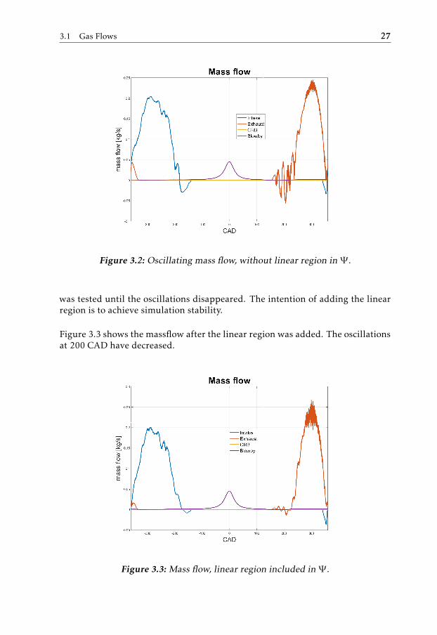
The simulated mass flow had oscillations. This was dealt with by including alinear region for the compressible flow, see Equation (2.42). In Figure 3.2 themass flow is shown before the linear region was added. The size of the region

3.1 Gas Flows 27

Figure 3.2: Oscillating mass flow, without linear region in Ψ .

was tested until the oscillations disappeared. The intention of adding the linearregion is to achieve simulation stability.

Figure 3.3 shows the massflow after the linear region was added. The oscillationsat 200 CAD have decreased.

Figure 3.3: Mass flow, linear region included in Ψ .

28 3 Modelling

3.1.2 Blowby Flow

The blowby flow has been modeled as a compressible flow. In this thesis therewhere no discharge coefficients measured for the blowby flow. Instead theeffective area AE was used as a tuning parameter to get a good match withmeasured pressure curve. Measurements at Scania have shown that the blowbyflow is affected by the temperature in the cylinder. The ring gap between pistonring and cylinder wall gets smaller when the temperature increases and thataffects the effective area in the flow equation. The temperature and pressurein the crankcase used in the compressible flow equation are set as ambienttemperature and pressure.

3.2 Gas Properties

The working fluid is the simplified air model discussed in equation (2.20) forthe motored pressure and VVB. The gas properties have been obtained fromthe NASA polynomials. Figure 3.4 shows simulated temperature in the cylinderat high load. It shows that the temperature is well within the interval for thecommon species in NASA polynomials wich is up to 5000 K.

Figure 3.4: Simulated temperature in the cylinder at full load.

Heywood (2019) concludes that the peak burned gas temperature in ICE is oforder 2500 K which is in accordance with the simulated temperature presentedin Figure 3.4.


3.2.1 Combustion Gas Properties

During combustion the gas properties are also affected by burned gases and astate is used to keep track of the mass fraction of air xair . The mass fractionof burned gases is xburned = 1 − xair . An assumption made is that the fuelused is cetane C16H34 wich has lower heating value QLHV = 44 MJ/kg and thestochiometric air/fuel ratio (A/F)s = 14.8 (Eriksson and Nielsen, 2014).

To be able to model the combustion an assumption is that the combustion isbetween air and hydrocarbons. The chemical reaction is thus the following:

nf uel CaHb︸︷︷︸Fuel

+nair (O2 + 3.773N2)︸︷︷︸Air

+nBurned

(aCO2 +

b2H2O + 3.773

(a +

b4

)N2

)︸︷︷︸

Burned

−→

(nf uel + nBurned

) (aCO2 +

b2H2O + 3.773

(a +

b4

)N2

)︸︷︷︸

Burned

+

+(nair − nf uel

(a +

b4

))(O2 + 3.773N2)︸︷︷︸

Air

(3.4)

The number of moles that is involved in the reaction is calculated at IVC.

ntot,air = 1 + 3.773 (3.5)

ntot,Burned = a +b2

+ 3.773 (3.6)

nair =mIV CxairMairntot,air

(3.7)

nf uel =mf uelMf uel

(3.8)

nBurned =(1 − xair )mIV C

MBurnedntot,Burned(3.9)

In the equations above mIV C denotes the mass in the cylinder at IVC.

xair is modeled as a state

dxairdt

=RTpV︸︷︷︸

1m

∑i

(xair,i − xair )mi − Cdxbdt

(3.10)

dxbdt correspond to the derivative of the Vibe function and C is a scaling of the

Vibe function to make sure that after the combustion the mass fraction of air isaccording to what is predicted in equation (3.4).

30 3 Modelling

In the equation above the sum corresponds to the filling and emptying of thecylinder. With xair,intake = 1 it is assumed that no residual gases are presentin the intake since the engine does not have EGR. It is only the filling of thecylinder and the combustion that affect the state, since it is assumed that thecompostion in the cylinder is homogeneous. The idea to model the mass fractionhas been used in Wahlström and Eriksson (2011) where they kept track of themass fraction of oxygen xO2

. If the flow goes from the cylinder to the intakemanifold the state xair is not altered since it is only the filling of the cylinder andcombustion that alters the state.

The molar fraction of xair after the combustion, (here it is assumed that thecombustion efficiency ηco = 1 since CI engines runs lean).

xair,af terCombustion =

(nair − nf uel

(a + b

4

))ntot,air(

nair − nf uel(a + b

4

))ntot,air +

(nBurned + nf uel

)ntot,Burned

(3.11)

Finally the mass fraction of air after combustion is calculated:

xair,af terCombustion =xairMair

(1 − xair )MBurned + xairMair(3.12)

The scaling of the Vibe function is thus:

C = xair,bef oreCombustion − xair,af terCombustion (3.13)

The gas mass specific gas constant has been calculated as

R = (1 − xair )RBurned + xairRair (3.14)

The mass specific heat at constant pressure have been calculated as

cp = (1 − xair )cp,Burned + xaircp,air (3.15)

where cp,air and cp,Burned have been obtained from the NASA polynomials andEquation (2.24b).

From the ideal gas assumption cv is obtained as

cv = cp − R (3.16)

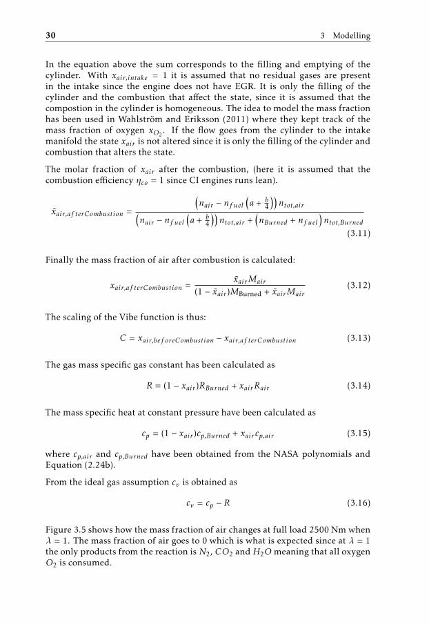
Figure 3.5 shows how the mass fraction of air changes at full load 2500 Nm whenλ = 1. The mass fraction of air goes to 0 which is what is expected since at λ = 1the only products from the reaction is N2, CO2 and H2O meaning that all oxygenO2 is consumed.

3.3 Heat Transfer 31

Figure 3.5: Mass fraction air at full load when λ = 1.

3.3 Heat Transfer

The empirical formula used to describe the convection heat transfer coefficient inthe cylinder is described in Chapter 3.3.1.

The cylinder wall tempreature Tw is for a fully warmed up engine 140◦Caccording to Guzzella and Onder (2010, p 335). That is the wall temperaturethat has been used in equation (2.43). In equation (2.43) it is assumed that thetemperature is homogeneous in the entire combustion chamber. Equation (2.7)calculates the instantaneous area of the combustion chamber depending on θ. Ithas here been assumed that the combustion chamber is a perfect cylinder. Thewall temperature in the cylinder will have lower temperature than the pistoncrown, however a simplification made is that the temperature is the same forpiston crown and the cylinder walls.

3.3.1 Woschni

A method to calculate the heat transfer coefficient was originally presented inWoschni (1967), however equation (3.17) is taken from Eriksson and Nielsen(2014):

h = C0B−0.2p0.8w0.8T −0.53 (3.17)

with C0 = 1.30 · 10−2.

32 3 Modelling

The characteristic velocity in equation (3.17) is given by the following expression:

w = C1Sp + C2V TivcVivcpivc

(p − pm) (3.18)

The expression only depends on the mean piston speed when there is nocombustion. The motored pressure and the cylinder pressure is in that case thesame. The mean piston speed is given from engine geometry and kinematics asthe following:

Sp =2aNe

60(3.19)

Table 3.1 describes how the constants in Woschni’s model change during thedifferent strokes in the four stroke cycle.

Table 3.1: Constants used in Woschni’s model.

Gas Exchange Compression Combustion and expansionC1 6.18 2.28 2.28C2 0 0 0.00324

The motored pressure is modelled well with a polytrope, κ is the polytropicexponent.

pm(θ) =

p(θ), θ ≤ θSOCp(θSOC)

(V (θSOC )V (θ)

)κ, θ > θSOC

(3.20)

For pm(θ) in Woschni the polytropic exponent κ have been assigned to a constantvalue. The value on κ was optimized from a motored cycle. This is because themodel should be as generic as possible and require as few calibrations as possiblefor different engine loads. Another way would be to use measured motoredpressure from an engine test cell as pm(θ) in equation (3.18).

3.4 Torque Model

A simple instanteneous engine torque model that neglects friction is presentedin Eriksson and Nielsen (2014) and it is the following

Me,i(θ) =

ncyl∑j=1

(pcyl,j (θ − θ0j ) − pamb)AL(θ − θ0

j ). (3.21)

θ0j denotes the individual offset of each cylinder. The pressure in the crank case

is set to the ambient pressure pamb = 1 [bar]. Note that the product of the area

3.4 Torque Model 33

and the crank lever is the same as the volume derivative with respect to crankangle see Equation (2.5).

AL(θ) =dVdθ

=dVdt

1ωe

(3.22)

The average torque obtained from the four strokes is of interest in for examplethe gearbox. A formula for calculating the average torque is the following:

Me =1

4π

4π∫0

Me,i(θ)dθ −Mf (3.23)

Mf denotes friction, which has been neglected in this thesis. The calculationsfrom the torque model have been performed from simulation on one cylinder.

4Data acquisition

This chapter describes the placement of the sensors used to acquire data andwhat type of measurement equipment that has been used to collect the data.There will also be a discussion on the physical principle of piezoelectric sensorsand how to deal with the problem of not knowing the absolute cylinder pressurefrom the cylinder pressure sensor. The data has been collected in an engine testcell at Scania CV AB. The measurements have been conducted at steady-stateconditions.

The measured cylinder pressure is crank angle resolved, however it needs anabsolute level on the pressure at some point in a cycle. Methods for that aredescribed in chapter 4.1. The manifold pressures are crank angle resolved, itis necessary due to the fact that the pressure varies during the cycle. Pressurevariations in the intake and exhaust manifolds are due to pulsations caused by theopening and closing of valves. The temperatures in the manifolds are averagedon all sensors during one cycle.

The measurements have been collected from an inline 6 cylinder Scaniaprototype engine with VVT and CRB. The cylinder pressure has been measuredin cylinder 6 because it is the cylinder that is the closest to the flywheel. Therethe torsion and crankshaft flexibility is the smallest and hence neglected. Thepressure in the intake manifold has been measured close to the inlet valve ofcylinder 6. The pressure in the exhaust manifold has been collected close to theexhaust valve of cylinder 6. Figure 4.1 shows a simplified sketch of the locationof the various sensors. Measurements have also been performed on cylinder 1but those have not been used in the cylinder model.

35

36 4 Data acquisition

Figure 4.1: An overview of the engine and its sensor locations.

Table 4.1: Description of measured signals used for input to the Simulinkmodel in this thesis.

Symbol Description UnitIphase Phasing of IVO and IVC. [CA]Ephase Phasing of EVO and EVC. [CA]mf Mass of fuel injected [kg]Ne Engine speed [RPM]pim(CAD) Intake manifold pressure [Pa]pem(CAD) Exhaust manifold pressure [Pa]SOI Start of injection [CA]Tim Intake manifold temperature [K]Tem Exhaust manifold temperature [K]

Table 4.2 describes the outputs from the Simulink model implemented in thisthesis.

Table 4.2: Outputs from the Simulink model.

Symbol DescriptiondTdt Temperature state.dpdt Pressure state.m Mass in the cylinder.dxairdt Mass fraction of air state.Mei Instantenous torque.Φcyl Φ in the cylinder at IVC.

4.1 Absolute Reference Of Cylinder Pressure 37

Table 4.3 presents signals used for evaluating the Simulink model. pcyl is themeasured cylinder pressure. λaf is evaluated from measurment of massflow ofair and fuel and it is assumed that the fuel is known to be able to obtain thestochimoetric (A/F)s value. Mf lywheel is the averaged torque measured at theflywheel.

Table 4.3: Description of signals used for evaluation.

Symbol Description Unitpcyl(CAD) Cylinder pressure [Pa]λaf Lambda [-]Mf lywheel Measured torque at the flywheel [Nm]

4.1 Absolute Reference Of Cylinder Pressure

The cylinder pressure is measured by a piezoelectric transducer. By design thetransducer responds to pressure differences by outputting a charge referenceto an arbitrary ground. This means that the transducer at some point must bedirectly correlated to pressure (Randolph, 1990). To get a useful signal from themeasurements a charge amplifier is needed. The charge amplifier is adjusted sothat a useful signal can be obtained. The adjustment is done so that the leakagecurrent is small. The signal from the amplifier decreases exponentially. Thatcan be used to reconstruct the true pressure curve. The knowledge that thederivative of an exponential is the same as the function itself means that the rateof which the signal decreases is propotional to the signal level. The signal fromthe charge amplifier measures relative change of the cylinder pressure well butnot the absolute value of the cylinder pressure (Johansson, 2003). In Johansson(2003) diffrent ways of chosing the absolute value for the cylinder pressure isdiscussed:

1. Set the cylinder pressure equal to the pressure in the intake manifold atBDC.

2. Set the cylinder pressure during the exhaust stroke equal to exhaustbackpressure.

3. Assume polytropic compression with known κ.

4. Assume polytropic compression with unknown κ.

The methods described in Johansson (2003) was evaluated in Randolph (1990),there they concluded that the best method was pegging at BDC. The methodworked best in untuned intake systems or at low speed in tuned systems. Tunedsystems means that the pulsating pressure waves from the exhaust system isappropretly arranged so that the wave will raise the nominal inlet pressure whichwill increase induced air in to the cylinder (Heywood, 2019). The uncertainty ofusing only one sample when pegging at BDC is removed by taking one samplebefore BDC and one after to avoid error from point measurements.

5Result and Discussion

The figures in this chapter will compare simulated results with cycle averagedresults from measurements. In Figure 5.1 a pressure curve from a high load caseis presented. As seen in the figure the pressure curve does not change much fromone cycle to another. Thereby a representative pressure curve is to average allpressure curves and compare the simulated pressure to that pressure curve. Allfigures in this Chapter that have CAD at the x-axis are plotted in the interval±360 CAD, where 0 CAD corresponds to TDC fire. The measurments used tovalidate the results have been measured at stationarity.

Figure 5.1: Pressure plot for 50 consecutive cycles at high load.

39

40 5 Result and Discussion

5.1 Motored Pressure

Figure 5.2: CAD pressure plot and effective valve flow area at 1400 RPM.

In the motored measurements the fuel have been cut off and an electric motorhave cranked the engine. Figure 5.2 shows the CAD pressure plot at 1400 RPMand the effective flow area AE for the intake and exhaust valve. In this caseIVO and EVO are the standard values and there is no phasing of the valves.The simulated pressure shows good agreement with the measured pressure see,Figures 5.2 and 5.3.

Figure 5.3 shows the pV-diagram for the motored case. In Figure 5.3 it is seen thatthe simulated pressure has a larger peak than the measured. The reason can bethat there are production tolerances in the compression ratio rc. The compressionpolytrope deviates from the measured as do the expansion polytrope. The reasonis most likely that the heat transfer model fails to model the true heat transfer inthe cylinder. The temperature is the same for cylinder wall and piston which isa potential source of error. Measurments at Scania have shown that the piston iswarmer compared to the cylinder walls. That in turn will affect the size of thering gap which will affect the effective flow area for the blowby flow. The averageindicated torque predicted by the simulink model is -146 Nm. The averagedmeasured torque at the flywheel was -161 Nm. The reason for the difference ismost likely that the torque model neglects friction and that the pV-diagram arenot exactly identical. Measured torque also includes friction and hence shouldbe slightly more negative.

Figure 5.4 shows the simulated massflows. The blowby flow is biggest at TDCsince the effective flow area is set as a small constant and that the cylinderpressure is largest at TDC for motored cycles. As expected the flow from the

5.1 Motored Pressure 41

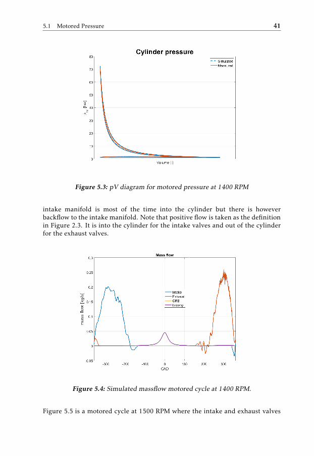
Figure 5.3: pV diagram for motored pressure at 1400 RPM

intake manifold is most of the time into the cylinder but there is howeverbackflow to the intake manifold. Note that positive flow is taken as the definitionin Figure 2.3. It is into the cylinder for the intake valves and out of the cylinderfor the exhaust valves.

Figure 5.4: Simulated massflow motored cycle at 1400 RPM.

Figure 5.5 is a motored cycle at 1500 RPM where the intake and exhaust valves


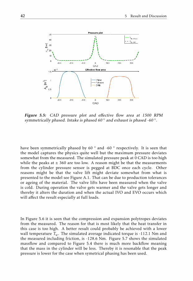
Figure 5.5: CAD pressure plot and effective flow area at 1500 RPMsymmetrically phased. Intake is phased 60 ◦ and exhaust is phased -60 ◦.

have been symmetrically phased by 60 ◦ and -60 ◦ respectively. It is seen thatthe model captures the physics quite well but the maximum pressure deviatessomewhat from the measured. The simulated pressure peak at 0 CAD is too highwhile the peaks at ± 360 are too low. A reason might be that the measurmentsfrom the cylinder pressure sensor is pegged at BDC once each cycle. Otherreasons might be that the valve lift might deviate somewhat from what ispresented to the model see Figure A.1. That can be due to production tolerancesor ageing of the material. The valve lifts have been measured when the valveis cold. During operation the valve gets warmer and the valve gets longer andthereby it alters the duration and when the actual IVO and EVO occurs whichwill affect the result especially at full loads.

In Figure 5.6 it is seen that the compression and expansion polytropes deviatesfrom the measured. The reason for that is most likely that the heat transfer inthis case is too high. A better result could probably be achieved with a lowerwall temperature Tw. The simulated average indicated torque is -112.1 Nm andthe measured including friction, is -128.6 Nm. Figure 5.7 shows the simulatedmassflow and compared to Figure 5.4 there is much more backflow meaningthat the mass in the cylinder will be less. Thereby it is resonable that the peakpressure is lower for the case when symetrical phasing has been used.

5.1 Motored Pressure 43

Figure 5.6: pV diagram for symmetrically phased 60◦ at 1500 RPM. Intakeis phased 60 ◦ and exhaust is phased -60 ◦.

Figure 5.7: Simulated massflow for symmetrically phased 60◦ at 1500 RPM.Intake is phased 60 ◦ and exhaust is phased -60 ◦.


5.2 CRB

Figure 5.8: Pressure CAD plot CRB 1000 RPM. The manifold pressures forintake and exhaust are seen. The intake manifold pressure is rather constantwhile the exhaust manifold pressure have pulses. The effective flow areashows that the CRB is activated.

This subchapter will discuss results from simulation compared to measuredcylinder pressure when CRB have been used. In Figures 5.8, 5.11, 5.10 and 5.13it is seen that CRB lift is also activated. In those Figures it is also seen that theCRB valve is open at the point where the cylinder pressure has its peaks. Thepressure ratios between exhaust manifold and cylinder pressure is well above5.5, seen in Figures 5.8 and 5.11. That is the maximum pressure ratio that hasbeen measured for the CD values for the exhaust valve, see Figure A.3. Anotheruncertainty is the valve lift since the pressure against the valve are much greaterthan in normal operation the lift profile will be altered and the opening of thevalve will most likely deviate more than in standard operation. It has beenobeserved at Scania in engine test cells that the valve lift is altered when thereis significant pressure ratios between cylinder pressure and manifold pressures.In Figures 5.9 and 5.12 it is seen that the peak pressure is too big and that thepressure following past ± 300 CAD is too low. The largest source of error is mostlikely that the CD values for exhaust are not measured for the significant pressureratios between cylinder pressure and exhaust manifold pressure. In Figures 5.10and 5.13 it is seen that the largest massflow is close to TDC. That is where thepressure ratios between cylinder pressure and exhaust manifold are the greatestand that is were the uncertainty of CD value and valve lift is most significant.In the pV-diagram, Figures 5.9 and 5.12, it is seen that the simulated pressurecaptures the physics somewhat but not the pressure peaks. The dashed blue line

5.2 CRB 45

Figure 5.9: pV diagram CRB 1000 RPM.

from the simulated which is higher then the solid is from bad inital conditionsfor temperature and pressure in the cylinder. The solid blue line is what the pV-diagram converges to after some simulations. The VVB measurement at 1000RPM had average indicated torque of -761 Nm and the simulated not includingfriction was -736 Nm. At 1700 RPM the measured indicated torque was -1700Nm and the simulated was -1716 Nm.

Figure 5.10: Simulated massflow CRB 1000 RPM.


Figure 5.11: Pressure CAD plot CRB 1700 RPM. The manifold pressures forintake and exhaust are seen. The intake manifold pressure is rather constantwhile the exhaust manifold pressure have pulses. The effective flow areashows that the CRB is activated.

Figure 5.12: pV diagram CRB 1700 RPM.

5.3 Combustion 47

Figure 5.13: Simulated massflow CRB 1700 RPM.

5.3 Combustion

In this subchapter the results obtained from combustion simulations arediscussed. The data have been collected in an engine cell at high load (∼250mg/stroke fuel), the difference between the two measurements is when theinjector needle starts to inject fuel. Meaning that start of injection (SOI) havebeen altered between the two different measurements. λmeasured and simulatedis also discussed in this subchapter. λ gives a hint on the trapped mass in thecylinder. That is if the mass of fuel mf and (A/F)s is known see the definition ofλ in equation (2.33). Thereby λ can give a hint how well the gas exchange workswithin the model.

Another measurement is at low load (∼38 mg/stroke fuel). In all combustionmeasurements discussed here the engine speed was 1200 RPM. In Figure 5.14the simulation captures the physics but one can clearly see that the simulatedpressure curve starts to burn too late. The measured λ in that case was 1.853while the simulated was 1.879. The reason for the difference might be thatsimulated and engine test cell might not use the same value of (A/F)s or thatthe estimated mass at IVC in the simulation might be a little off. In the pV-diagram Figure 5.15 it is seen that both the gas exchange as well as the peakpressure is captured, however the expansion polytrope is somewhat off comparedto the measured. Compared to previous massflows the massflow in Figure 5.16is much greater. That is mostly due to that fact that the pim pressure is greateras consequence of the increase in boost pressure from the turbocharger. Themeasured indicated torque was 2499 Nm and the simulated was 2560 Nm fromFigure 5.15. Figure 5.17 shows the massfraction of air, when the combustionstarts the massfraction of air decreases. At IVO the cylinder is filled with fresh


Figure 5.14: CAD pressure plot for high load 2500 Nm.

air wich increases the mass fraction of air as seen in the Figure.

The simulated pressure curve in Figure 5.18 shows the cad pressure curve andeffective flow area at high load at 1200 RPM. The simulated pressure curvecaptures the shape of the measured pressure somewhat. The pressure increasedue to combustion is too large in the simulated case. That is most likely due tothat Diesel combustion needs at least a double Vibe to be modeled accurately.That is due to the fact that there is a premix and a main burning which cannotbe accurately described by a single Vibe. Even though that the pV diagram inFigure 5.19 deviates somewhat from the measured, the average indicated torquesmeasured and simulated are quite close, 2501 Nm and 2572 Nm respectively. Themeasured λ was 1.898 and the simulated was 1.917, thereby the simulated andmeasured is close. The torque deviates due to that the torque is measured at theflywheel and thereby friction losses is most likely obtained.

In Figure 5.21 it is seen that the simulated pressure follows both the expansionand compression curve well, but the simulated pressure does not capture thepressure peak. The reason is most likely due to the fact that Matekunas pressureratio method fails to make an accurate heat release in this case. The pressuredifference from compression and combustion in this case is not much at alland thereby a small error in the polytrope in Matekunas will fail to predict anaccurate heat release. In the two previous combustion data sets the injectedfuel was ∼250 mg/stroke compared to ∼38 mg/stroke here. In Figure 5.22 itis seen that the gas exchange is well captured by the simulation even though itfails to predict the peak pressure. The gas exchange happens when there is aneffective flow area. In those regions in Figure 5.21 the simulated and measuredpressure are essentially the same. The simulated massflow in Figure 5.23 shows

5.3 Combustion 49

Figure 5.15: pV diagram for high load 2500 Nm.

Figure 5.16: Simulated massflow for high load 2500 Nm.


Figure 5.17: Mass fraction of air at high load 2500 Nm.

Figure 5.18: CAD pressure plot for high load 2500 Nm.

5.3 Combustion 51

Figure 5.19: pV diagram for high load 2500 Nm.

Figure 5.20: Simulated massflow for high load 2500 Nm.


oscillations in the mass flow from the intake valve which suggest that the pressurein the intake manifold and the cylinder are close to each other causing numericinstabilities as described in Chapter 2.6.1. The measured indicated torque fromFigure 5.22 was 171 Nm and the simulated was 182.2 Nm.

Figure 5.21: CAD pressure plot for low load 170 Nm.

Figure 5.22: pV diagram for low load 170 Nm.

5.3 Combustion 53

Figure 5.23: Simulated massflow for low load 170 Nm.

In Figure 5.24 it is seen that the mass fraction of air does not increase at IVO.That has to do with the fact that there is backflow to the intake manifold. Hencethere is no flow of fresh air into the cylinder, and with the assumption that themixture is homogeneous the mass fraction of air is unaltered.

Figure 5.24: Mass fraction air for low load 170 Nm.


5.4 Real Time Feasibility Study

The purpose of this study was to see if it is possible to implement the model ona HIL environment for functional testing and if it is possible to implement on anECU. The test was performed on a data set with combustion. The runtime wasestimated by using Tic and Toc in Matlab. To be able to get as realistic resultas possible the Simulink model was built before the run time estimation wasperfomed. That was solved in Simulink by the use of enable fast restart.The runtime for different solvers and step lengths are presented in Table 5.1. Thetest used here only used fixed step length and that is essential for implementationon ECU but not required on HIL. The simulation time obtained and the steplengths used, suggest that it is possible to implement the model on a HILenvironment and on an ECU by code optimization.

Table 5.1: Runtime for different solvers on the simulink model on a portablecomputer with Intel I5 2.5 GHz 8GB RAM, the simulation time was set to 1second. By fail it is meant that the simulation crashes.

Step length h ODE1 [s] ODE2 [s] ODE4 [s]4 · 10−4 fail fail fail3 · 10−4 fail 0.98 1.012 · 10−4 1.03 1.08 1.141 · 10−4 1.31 1.43 1.995 · 10−5 1.78 2.15 3.241 · 10−5 6.27 7.36 10

6Future Work

The valve lifts discussed in this thesis have been measured for a cold engine andby turning the camshaft two revolutions. However as the engine gets warmerthe valves get longer and thereby does not agree with the measured valve lifts.Fortunantely there are methods to compensate for that, for instance by hydrauliclash adjusters (HLA). The HLA reduces the maintenance significantly, as the needfor periodically adjusting the valve lash disappear (Phlips and Schamel, 1991).The valve lift affects the mass flow through the ports and thereby it is essentialto know the true valve lift. By using HLA, EVO and IVO can be more accuratelydetermined.

The CD values needs to be measured for larger pressure ratios for the exhaustvalve. There is also a need to make transient measurements. It has beenconcluded in Winroth et al. (2018) that the CD values measured from stationarymeasurements are overestimated. By transient experiment it is meant that the airflow rig uses the same valve motion and under the same conditions as an enginewould have done. The stationary measurements are that the valve is lifted intoposition and the massflow is observed when it has reached a static level.

The Simulink model uses the temperature in the exhuast manifold as inputand uses it for the flow calculation at the exhaust port. The engine studied inthis thesis had temperature sensors at the exhaust ports however the enginesin production does not. Thereby a model for the temperature in the exhaustmanifold would be necessary. It would be interesting to perfom a sensitivityanalysis and see how important it is to get the temperature correct or if it is goodenough to set the temperature to a constant.

A further investigation of this thesis would also be to implement the model in anECU and see if it is possible to do so from the step lengths needed for the model.

55

56 6 Future Work

In this thesis a goal was that the model should use the same set of equationsfor all different parts of the four stroke cycle. From an ECUs point of view it isgood, because the simulation time will not vary as much as if there were differentcalculations for the different cases. The model as of now does its calculations inthe time domain. A simple scaling of 1

ωeis what is needed to change the model

to calculate in the crank angle domain. A limitation if the model would calculatein the crank angle domain would be how to handle the case when the enginespeed ωe = 0. That is not a problem for the Simulink model since it is in the timedomain.

A state for piston temperature and wall temperature is needed to get a better heattransfer model. The piston temperature will affect the ring gap which in turn willaffect the blowby flow. An investigation on how the ring gap affect the blowbyflow would be interesting. The wall temperature could by knowing material andthe temperature in the cylinder act as a state as for piston temperature. Guzzellaand Onder (2010) suggests that the wall temperature Tw can be estimated bylooking at the increase in temperature in the coolant and from knowing thecoolants flow rate.

In Chapter 2.9 it is described that diesel combustion in DI engines requiresat least a double Vibe to accurately model the combustion. To be able toparameterise those two Vibe functions a more accurate heat release analysis hasto be performed, for example by studying the gross heat release which comparedto the net heat release also considers contribution from heat transfer. A moreaccurate way to determine the SOC is also required either by using the modelsfor ignition delay from chapter 2.8.1 or by analysing cylinder pressure data.

Another interesting investigation would be to run the simulation model on theother cylinders that are not closest to the flywheel. Thereby it could be seen howsensitive the model is for the torsion and flexibility in the crankshaft.

Finally a modification that the instantaneous volume V is not only dependent onθ but also pcyl . That because the instantaneous cylinder volume can deviate asmuch as 6% from the geometrical at TDC at high load (Anagrius West et al., 2018).At high load the forces acting on the piston makes the piston deviate somewhatfrom its provided geometrical data.

Appendix

AModel Parameters

This appendix presents some of the different model parameters that have beenused in this thesis.

A.1 Gas Properties

Table A.1 show the mole mass for some common species. Atmospheric nitrogenis that the gases that makes up air except for oxygen have been lumped intonitrogen. The air model in equation (2.20) gives the following molar mass for air:

Mair =1

1 + 3.773(1 · 32 + 3.773 · 28.16) = 28.96 [g/mole] (A.1)

The mole mass for the burned gases is (assuming that cetane is the fuel a=16,b=34):

MBurned =1

a + b2 + 3.773(a + b

4 )(aMCO2

+b2MH2O + 3.773(a +

b4

)MN2) =

=1

16 + 17 + 3.773 · (16 + 34/4)(16 · 44.01 + 17 · 18.02 + 3.773 · (16 + 34/4) · 28.16) =

= 28.81 [g/mole] (A.2)

Since the mole mass of air and burned gases do not differ much the mass specificgas constant R is roughly the same for air as for burned gases.

59

60 A Model Parameters

Table A.1: Molar mass from species taken from Heywood (2019).

Specie Molecular weight [g/mole]Carbon C 12.011Hydrogen H2 2.016Cetane C16H34 226.44Oxygen O2 32.00Atmospheric Nitrogen N2 28.16Carbon dioxide CO2 44.01Water H2O 18.02

A.2 Valve Properties

The valve lift profiles Lv shown in Figure A.1 is used when calculating the CDvalues for exhaust, intake and CRB. The lift profile for CRB and exhaust athigh pressure ratios will differ from the values obtained from the look up table,however that has not been considered in the implementation. The CD valuesdisplayed in Figures A.2 and A.3 have been measured at steady flow experiments.

Figure A.1: Valve lift for the different valves note that TDC fire is at 360 ◦.

A.2 Valve Properties 61

Figure A.2: CD value for intake valve as a function of Lv/Dv

Figure A.3: CD value for exhaust valve as a function of Lv/Dv and Pr(pressure ratio).

Bibliography

Ivan Anagrius West, Carlos Jorques Moreno, Ola Stenlåås, Fredrik Haslestad, andOla Jönsson. Internal combustion engine cylinder volume trace deviation, apr2018. Cited on pages 8 and 56.

Yunus A. Cengel, Mehmet Kanoglu, John M. Cimbala, and Robert H. Turner.Fundamentals of thermal-fluid sciences. McGraw-Hill Education, 5 th edition,2017. Cited on pages 8, 11, and 18.

C Lyle Cummins. Jacobs Engine Brake Retarder, Bloomfield, Conneticut.American Society of Mechanical Engineers, 1985. Cited on page 17.

Thomas Dresner and Philip Barkan. A review of variable valve timing benefitsand modes of operation. In 1989 Conference and Exposition on FutureTransportation Technology. SAE International, aug 1989. Cited on page 17.

Rolf Egnell. The influence of egr on heat release rate and no formation in a didiesel engine. In CEC/SAE Spring Fuels & Lubricants Meeting & Exposition.SAE International, jun 2000. Cited on page 2.

Asko Ellman and Robert Piché. A two regime orifice flow formula for numericalsimulation. Journal of Dynamic Systems Measurement and Control, 121:721–724, 12 1999. Cited on page 16.

Lars Eriksson. CHEPP – A Chemical Equilibrium Program Package for Matlab.SAE Transactions, Journal of Fuels and Lubricants, 2004-01-1460, 4(113):730–741, June 2005. Cited on page 14.

Lars Eriksson and Ingemar Andersson. An analytic model for cylinder pressurein a four stroke si engine. SAE Transactions, 111:726, 2002. Cited on pages 2and 23.

Lars Eriksson and Lars Nielsen. Modeling and control of engines and drivelines.Automotive series. Chichester, West Sussex, U.K. : John Wiley and Sons Ltd,2014. Cited on pages 6, 7, 11, 14, 15, 16, 18, 19, 20, 21, 23, 29, 31, and 32.

63

64 Bibliography

J. A. Gatowski, E. N. Balles, K. M. Chun, F. E. Nelson, J. A. Ekchian, andJohn B. Heywood. Heat release analysis of engine pressure data. In 1984SAE International Fall Fuels and Lubricants Meeting and Exhibition. SAEInternational, oct 1984. Cited on pages 2 and 14.

L. Guzzella and Christopher H. Onder. Introduction to modeling and control ofinternal combustion engine systems. Springer, 2010. Cited on pages 31 and 56.

H.O. Hardenberg and F. W. Hase. An empirical formula for computing thepressure rise delay of a fuel from its cetane number and from the relevantparameters of direct-injection diesel engines. In 1979 Automotive EngineeringCongress and Exposition. SAE International, feb 1979. Cited on page 18.

John Heywood. Internal Combustion Engine Fundamentals 2E. New York, N.Y.: McGraw-Hill Education., 2019. Cited on pages 8, 10, 15, 17, 18, 19, 28, 37,and 60.

Bonnie J. McBride, Michael J. Zehe, and Sanford Gordon. Nasa glenn coefficientsfor calculating thermodynamic properties of individual species. 10 2002. Citedon page 13.

Bengt Johansson. Förbränningsmotorer del 2. Lund : Institutionen för värme-och kraftteknik, Lunds tekniska högskola, 2003, 2003. Cited on page 37.

Bengt Johansson. Combustion engines volume I. Lund : Lund University ;Stockholm : Kungliga Tekniska Högskolan, KTH, 2017. Cited on page 10.

Felicia Åkerman. Eu:s ledare och parlamentet överens om krav påminskade utsläpp från lastbilar. Dagens industri, feb 19 2019.https://www.di.se/live/eus-ledare-och-parlamentet-overens-om-krav-pa-minskade-utslapp-fran-lastbilar/ accessed: 2019-02-20. Cited on page1.

Marcus Klein and Lars Eriksson. A specific heat ratio model for single-zone heatrelease models. In SAE 2004 World Congress & Exhibition. SAE International,mar 2004. Cited on page 14.

Markus Klein. Single-zone cylinder pressure modeling and estimation for heatrelease analysis of SI engines. Linköping studies in science and technology:Dissertations 1124. Linköping : Department of Electrical Engineering,Linköping University, 2007, 2007. Cited on pages 2 and 22.

R.B. Krieger and G.L. Borman. The Computation of Apparent Heat Releasefor Internal Combustion Engines. American Society of Mechanical Engineers.ASME, 1966. Cited on pages 2 and 20.

Patrick Phlips and Andreas Schamel. The dynamics of valvetrains withhydraulic lash adjusters and the interaction with the gas exchange process. InInternational Congress & Exposition. SAE International, feb 1991. Cited onpage 55.

Bibliography 65

Andrew L. Randolph. Methods of processing cylinder-pressure transducersignals to maximize data accuracy. In International Congress & Exposition.SAE International, feb 1990. Cited on page 37.

Gerald Rassweiler and Lloyd Withrow. Motion pictures of engine flamescorrelated with pressure cards. In Annual Meeting of the Society. SAEInternational, jan 1938. Cited on pages 2 and 21.

Mark C. Sellnau, Frederic A. Matekunas, Paul A. Battiston, Chen-Fang Chang,and David R. Lancaster. Cylinder-pressure-based engine control usingpressure-ratio-management and low-cost non-intrusive cylinder pressuresensors. In SAE 2000 World Congress. SAE International, mar 2000. Citedon page 2.

Peter Templin. A diesel engine model, including compression brake for,powertrain control. In International Truck and Bus Meeting and Exhibition.SAE International, nov 2002. Cited on page 2.

Ivan I Vibe and Franz Meißner. Brennverlauf und kreisprozess vonverbrennungsmotoren. Verlag Technik, 1970. German translation of therussian original. Cited on page 2.

Johan Wahlström and Lars Eriksson. Modelling diesel engines with a variable-geometry turbocharger and exhaust gas recirculation by optimization ofmodel parameters for capturing non-linear system dynamics. Proceedingsof the Institution of Mechanical Engineers, Part D, Journal of AutomobileEngineering, 225(7):960–986, 2011. Cited on page 30.

Marcus Winroth, C L. Ford, and Per-Henrik Alfredsson. On discharge frompoppet valves: effects of pressure and system dynamics. Experiments in Fluids,59, feb 2018. Cited on page 55.

G. Woschni. A universally applicable equation for the instantaneous heat transfercoefficient in the internal combustion engine. In National Fuels and Lubricants,Powerplants, Transportation Meetings. SAE International, feb 1967. Cited onpages 2 and 31.

full cycle cylinder state estimation in di engines with...

Documents