full cost analysis of accessibility

Full cost analysis of accessibility1

Mengying Cui2University of Minnesota3Department of Civil, Environmental, and Geo- Engineering4500 Pillsbury Drive SE5Minneapolis, MN 55455 [email protected]

David Levinson8RP Braun-CTS Chair of Transportation Engineering9Director of Network, Economics, and Urban Systems Research Group10University of Minnesota11Department of Civil, Environmental, and Geo- Engineering12500 Pillsbury Drive SE13Minneapolis, MN 55455 [email protected]

4493words + 9 figures + 2 tables=7243words16July 25, 201617

ABSTRACT1Traditional accessibility evaluation fails to fully capture the travel costs, especially the external2costs of travel. This study develops a framework of extending accessibility analysis combining3the alternate (internal and external) cost components of travel, time, safety, emission and money,4with accessibility analysis, which makes it an efficient evaluation tool for the potential needs of5transport planning projects. An illustration of this framework based on a toy network was also6built in this paper, which proves the potential of applying the extending accessibility analysis into7the network of metropolitan areas.8

Mengying Cui and David Levinson 2

INTRODUCTION1Transport systems provide opportunities for people to participate in activities that are distributed2over space and time. The ease of reaching the activities implies a way to evaluate the performance3of transport systems, which we called accessibility (1).4

The term "accessibility" reflects the correlations between the cost and benefits of travel and5combines them into a single metric, which represents the strengths and weaknesses of interactions6of the transport network and land-use, that should be considered in transport planning.7

A very basic accessibility metric is cumulative opportunities, which measures the number8of opportunities reachable within a given threshold (2, 3). Figure 1 displays the accessibility to9jobs with a given time threshold setting as 20, 30, and 40 minutes respectively, based on the10cumulative opportunity measure. It illustrates the trade-off between a traveler’s willingness to pay11and benefit that can be achieved since an increased travel time threshold allows reaching more job12opportunities overall, where the travel time threshold represents a given time cost of travel.13

Nexus Research Group

0-1,0001,000-2,5002,500-5,0005,000-7,5007,500-10,00010,000-25,00025,000-50,00050,000-75,00075,000-100,000100,000-250,000250,000-500,000500,000-750,000750,000-1,000,0001,000,000-Highways

Job accessibility based onthe shortest travel time path within the

time threshold of 20min

Zone Structure Displayed: Transportation Analysis ZonePrimary Data Resources: Tom Tom Speed Data, Metropolitan Council

(a) Job Accessibility in 20 Minutes


0-1,0001,000-2,5002,500-5,0005,000-7,5007,500-10,00010,000-25,00025,000-50,00050,000-75,00075,000-100,000100,000-250,000250,000-500,000500,000-750,000750,000-1,000,0001,000,000-Highways




(b) Job Accessibility in 30 Minutes


0-1,0001,000-2,5002,500-5,0005,000-7,5007,500-10,00010,000-25,00025,000-50,00050,000-75,00075,000-100,000100,000-250,000250,000-500,000500,000-750,000750,000-1,000,0001,000,000-Highways




(c) Job Accessibility in 40 Minutes

FIGURE 1 : Job Accessibility in Different Time Thresholds Using Median Speeds

Accessibility is a reliable tool for comparing the effectiveness of proposed land-use and14transport network scenarios in planning projects. Anderson et al. (4) analyzed the accessibility15


of scenarios with the combination of six land use and twelve networks cases (both highway and1transit). Moreover, accessibility significantly affects different aspects of travel behavior. Levinson2(5) and Kockelman (6) examined the critical influences of accessibility on travelers’ behaviors of3commuting duration, vehicle kilometers traveled, automobile ownership, mode choice, etc. while4others have considered real estate prices and economic productivity (7).5

Most commonly, accessibility metrics have been analyzed from the perspective of the mean6or expected travel time by considering the time cost of travel (8). It is thought reasonable not only7because time cost is the key cost component affecting travelers’ choice of mode, route, and depar-8ture time, but also because the time cost is easier to understand and assess. But using only time9cost cannot capture the complete internal costs of travel since it disregards the cost factors from10crashes, pollution intake, and out-of-pocket money cost, which may affect travelers’ decisions,11and external costs from crashes and pollution emissions, which are significant though not affecting12traveler decisions in the absence of specific policies.13

Private or internal cost refers to what consumers pay directly for goods or services (in14transportation this is most typically enumerated in travel time, but also considers costs, pollution15intake, and crash risk). Rational economic agents are often assumed to choose the lowest private16cost during decision-making (9). However, an externality1 occurs when an agent engages in an17activity that affects the well-being of a bystander, but neither pays nor receives any compensation18for that effect (10).19

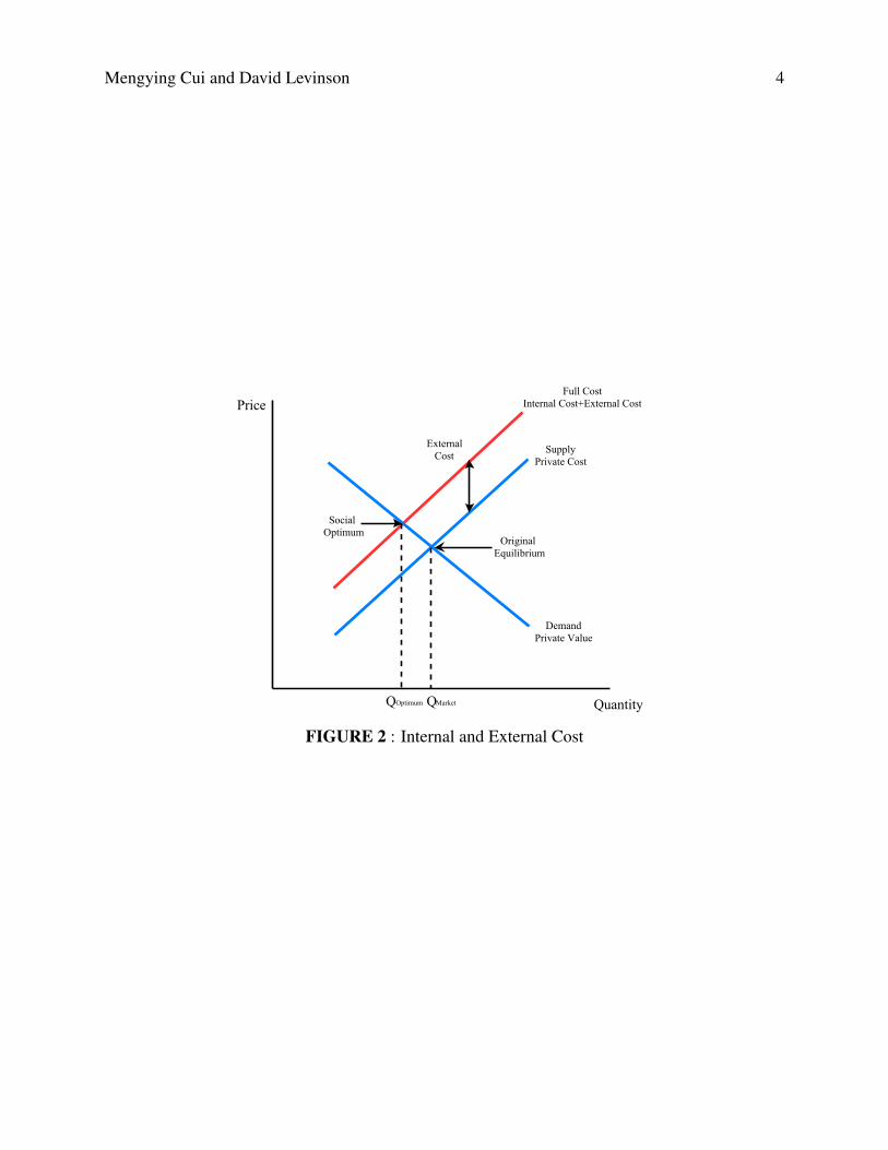
An externality could be positive if the activity is beneficial for bystanders. More often,20it is negative when it results in an adverse impact. Typically in transportation this is congestion21imposed on others, increased crash risk to others, pollution emissions, and road wear and tear in22excess of road charges. With the development of motorized transport system, external costs from23crashes, environmental damage, and unproductive travel time cannot be ignored. Both internal and24external costs should be measured for full cost (the sum of internal and external cost) analysis (11).25

Figure 2 (Source: Mankiw (10)) shows the relationship between internal and external cost.26Internalizing the externality (for instance with a Pigouvian Tax) is one way social planners27

use to achieve a social optimum where individual consumers consider what otherwise would be28the external costs of their actions when taking decisions.29

Hence, in this paper, we built a framework of extending accessibility analysis based on30the full cost of travel. It could be used to investigate the alternative cost components during local31traveling considering both internal and external part of costs, to explore how each cost compo-32nent or their combinations play in travelers’ choice, and to evaluate accessibility accommodating33the potential planning needs by applying alternate costs components and their combinations into34accessibility metrics.35

The framework of extending accessibility analysis, methodology, an illustration of the36method and the conclusion are shown in Section 3-6 in turn.37

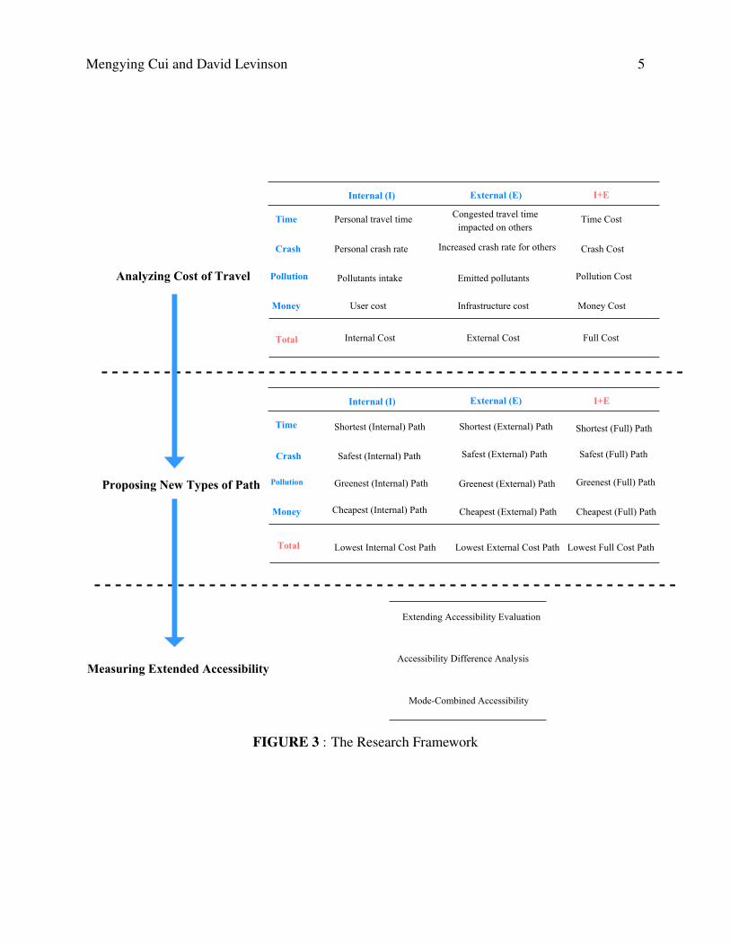
EXTENDING ACCESSIBILITY ANALYSIS38Extending accessibility analysis based on full cost of travel includes three steps: analyzing cost39of travel, proposing new types of paths and measuring extended accessibility, which follows the40framework shown in Figure 3.41

1An external cost is sometimes referred to as a ’social’ cost, however we do not use the term to avoid confusion, as’social’ cost sometimes also refers to the combination of internal and external costs. Instead, we use full costs for thecombined internal plus external costs, and externality or external cost for the costs the traveler does not bear.


FIGURE 2 : Internal and External Cost


FIGURE 3 : The Research Framework


Cost Analysis1In full cost analysis, the selected alternative cost components includes time, crashes, emissions, and2money, which all contain internal and external parts. Analyzing the travel costs at the individual3level (disregarding the social benefit of transport systems overall), almost all the externalities are4negative.5

Travel time can be divided into congested and uncongested components, in which con-6gested time implies the external cost imposed by others from the point-of-view of travelers since7additional vehicle on the roadways could result in incremental delay borne by others (following8travelers) (9). Hence, considering the link properties, traffic and capacity, the marginal cost of9travel time could be used to measure the external time cost.2 The total travel time for a trip borne10by the traveler is classified as internal time costs.11

For crash cost, similar to travel time, internal crash costs is generated by the personal crash12rate, borne by each traveler (it may be paid for via insurance policies) which refers to the number13of crashes per vehicle kilometer traveled. It covers both direct and indirect costs (11, 12). Each14traveler also increases the crash risk for others, this marginal increase of crash rate is an external15cost that should be paid by others (13).16

On-road emission is more likely to be categorized into external costs, which affect human17health, vegetation, materials, aquatic ecosystems, visibility, climate changes, e.g (14). Notably,18damage to human health due to air pollution is the most expensive element. Hence, the external19cost of emission from the perspective of travelers could be measured by the health damage cost20from emitted pollutants imposing on others. Moreover, as an active agent in transportation systems,21the health risk of travelers due to exposure to pollutants is considered as the internal emission costs22to travelers, which could be measured by the quantity of pollution intake (breathed in, in the case23of air pollution).24

The monetary cost of travel mainly includes user cost and infrastructure cost (if we avoid25double-counting for insurance and crashes). The user monetary cost (for fuel, vehicle ownership26and maintenance, tolls and taxes and fares, and the like) could be treated as an internal cost. The27external monetary costs mainly comprise the infrastructure costs, such as wear and tear on the road28or on a transit vehicle (net of the amount paid for in user fees and taxes to avoid double counting).29

With sufficiently high taxes (e.g. on fuel) it is certainly possible for there to be no net30external costs, however that is empirically not the case in the US at this time.31

Hence, the total costs for each cost components can be measured as the sum of the in-32ternal and external part of the corresponding costs, and the full costs would be the sum of the33corresponding costs from all the alternative cost components. To make sure each element in the34cost analysis table are additive, all these cost elements would be monetized based on standard cost35values, personal information, and link properties.36

The objective of the cost analysis is to provide a method to estimate the internal, external37and full costs of link segments, and aggregate this to the scale of a complete road network based38on travelers’ properties. The estimates could be used as link properties to measure the internal,39external and full costs of actual trips with given modes and routes, provide a measure to evaluate40the effectiveness of transport network, and show the potential to apply alternative costs components41into accessibility analysis.42

2From the perspective of the road system, the congested time (delay) is fully internalized, however for each traveler,which is the relevant decision unit here, it is an internal cost.


Definition of new types of paths1For each alternative cost component, two new path concepts are proposed: safest path and greenest2path, in addition to the traditional shortest time and least cost paths.3

• Shortest time path - the route with the lowest travel time costs.4

Shortest time (internal) (Pt,i) path is to minimize the private cost borne by travelers them-5selves, which is equivalent to the User Equilibrium (UE) path. And the external cost6complement aims to minimize the congestion cost imposed on others, and is referred to7as the "Shortest time (external) path" (Pt,e). The traditional socially optimal (SO) path8considering travel times would be the full cost version of this (Pt, f ).9

• Safest path - the route with the lowest crash costs.10

The safest path could provide the safety evaluation in the scale of the whole road net-11work, and shows the crash cost savings comparing with crash costs by using other paths12(e.g. shortest time path). But it could not be used alone to reflect travelers’ actual route13choices accurately (as most travelers wouldn’t know this anyway, even if they valued14safety highly). Safest (internal) path (Ps,i) and Safest (external) (Ps,e) path consider the15personal crash costs and crash costs imposed on others separately. The safest full cost is16denoted by (Ps, f ).17

• Greenest path - the route with the lowest emission costs.18

Greenest (internal) path (Pg,i) minimizes intake of on-road emissions. A complement to19this, Greenest (external) path (Pg,e) is the route with the lowest pollution costs consider-20ing emitted pollutants. Similarly, the greenest path is not the major concern for travelers21when they make decisions on route choice (and again few would know what this was),22as the safest path, but it provides the evaluation of on-road emissions overall and a mea-23surement of emission cost savings if travelers take pollution indexes into consideration24on their route choice, which could be achieved with Pigouvian Prices. The greenest full25cost path may differ from the greenest external cost path since pollution intake may also26include non-transportation sources, and would be denoted as (Pg, f ).27

• Cheapest (least expensive) path - the route with the lowest monetary costs.28

Again there are internal (Pl,i) and external (Pl,e) and full cost (Pl, f ) versions of this.29

The total internal, external and full costs of travel would also be considered as shown in30Figure 3. Most importantly, the lowest internal costs path fully consider the cost components31travelers care about, which explains travelers’ route choice behavior more accurately and makes32it feasible to assess the traffic flow based on the OD distribution. Moreover, the full cost savings33could be measured by comparing the travel costs of the lowest internal and full cost paths, which34shows the benefits that would be attained if travelers were to consider the external costs imposed35on others into their decisions.36

Accessibility Analysis37Extending accessibility analysis aims to pursue three final goals as below:38


• Accessibility Evaluation1

Accessibility evaluation develops a new type of accessibility analysis for each of the new2cost components. The number of jobs that can be reached in (e.g.) $0.20 of pollution3intake costs can be computed for both traditional shortest path as well as the new greenest4path. The similar calculation could be conducted for crash and monetary costs, for both5internal, external and full costs, and for auto and non-auto travel. See Figure 2.6

• Accessibility Difference Analysis7

Accessibility difference measures the penalties (in terms of reduction in the number of8destinations that can be reached for a given cost) to pursue the optimal path from one9aspect (shortest time, safest, or greenest path, for instance) rather than another within the10same cost threshold. Accessibility difference analysis could be measured by comparing11the accessibility metrics based on different cost components, or the internal and external12part for each of them. Most importantly, the comparison of accessibility metrics in the13realm of total internal and external costs explains the trade-off of the costs and benefits14between private and public. Travelers, for instance, could reach fewer job opportunities15to minimize the full cost with the same accepted cost threshold.16

• Mode-combined accessibility analysis17

Generally, accessibility analysis is separated by different traffic modes (auto, transit,18walk, or bike), which measures the ability to reach opportunities with a given mode19to travel. For the conventional accessibility measurement, the analysis is hard to be com-20bined since travel time usually represents the costs of trips and the order of needed travel21time for these modes is clear in most contexts (Walking > Bicycling > Transit > Autos).22Hence, the analysis is still only based on single mode, auto.23

Based on the full-costs of travel, the selected traffic mode would be the one with the24minimum total costs for a given OD pair. While this depends on the outcomes of the cost25analysis and the context, in general, considering other cost components makes non-auto26modes more competitive than when considering only private travel time cost. Apply-27ing the minimum total cost into the cost function provides a way to measure the mode-28combined accessibility.29

A mode-combined accessibility analysis gives a comprehensive evaluation on the effec-30tiveness of network operation. Considering access to jobs, a full-cost minimizing multi-31modal accessibility analysis could be conducted for the Metropolitan areas, finding for32each OD pair the mode with the lowest full composite cost.33

METHODOLOGY34The basic process of extending accessibility analysis is following the flowchart shown in Figure354, which, as mentioned, includes analyzing cost of travel (Blue Part), proposing new types of path36(Red Part) and measuring extended accessibility (Purple Part).37


FIGURE 4 : Process of Extending Accessibility Analysis


In cost analysis, time, crash, emissions, and money (infrastructure) are the key cost com-1ponents of travel during trips. For each component, the standard unit cost, such as value of travel2time per hour, cost per crash (or per fatality/injury), health damage cost and climate change costs3per ton of pollutants e.g., should be identified (from the literature), and the quantity of that cost4should be estimated (from transportation analysis) first.5

The unit costs vary across modes and population. In addition, considering the variates of6traffic conditions on different links, the properties of links, modes, and populations then are used to7calibrate the travel cost, which give each link a cost on the network with both internal and external8part.9

The new types of path are proposed based on each component of the link-based full cost10model and its composite considering both internal and external cost, with a basic assumption that11travelers are willing to optimize(minimize) the travel cost from different perspectives.12

All types of path could be applied into accessibility evaluation by comparing the cumulative13travel cost with the corresponding predetermined cost threshold (an assumed willingness-to-pay),14such as the shortest path with the time cost threshold, or the safest path with the crash cost thresh-15old. Accessibility differences could be measured comparing the accessibility metrics based on16different types of path, shortest path vs.lowest internal cost path, e.g., which reflects the influences17of travelers’ route choice on the cost of travel and, then, the accessibility.18

A mode-combined accessibility analysis could be conducted based on the lowest internal19cost path and the lowest full cost path considering travelers’ decisions on mode choice. The basic20hypothesis is that travelers will select the traffic mode with the lowest cost for a given OD pair.21The travel cost of the selected mode is used to compared with the predetermined cost threshold to22calculate the accessibility.23

24The basic functions used in the study of extending accessibility analysis include,25

• New types of paths26

The new types of paths were proposed as the route with the lowest corresponding cost27between a given OD pair considering different cost components or their combinations,28which could be expressed as,29

Ck,OD,c,m = ∑i∈Pk,OD,m

Ci,c,m (1)

30COD,c,m = min(Ck,OD,c,m) (2)

Where:31Ci,c,m is the cost of cost component c on link i by mode m,32Pk,OD,m refers to the kth path between origin O and destination D, by mode m,33k is selected from shortest time (t), safest (s), greenest (g), and least expensive (l) or34combined (c) paths considering internal (i), external (e), or full ( f ) costs35Ck,OD,c,m is the travel cost of the kth path considering cost component c, by mode m,36COD,c,m stands for the minimum travel cost between O and D considering cost component37c, by mode m.38


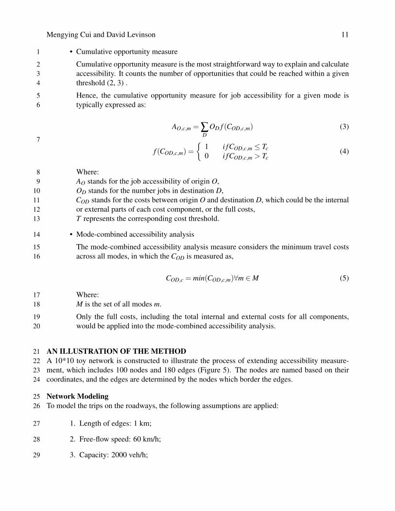
• Cumulative opportunity measure1

Cumulative opportunity measure is the most straightforward way to explain and calculate2accessibility. It counts the number of opportunities that could be reached within a given3threshold (2, 3) .4

Hence, the cumulative opportunity measure for job accessibility for a given mode is5typically expressed as:6

AO,c,m = ∑D

OD f (COD,c,m) (3)

7

f (COD,c,m) =

{1 i fCOD,c,m ≤ Tc0 i fCOD,c,m > Tc

(4)

Where:8AO stands for the job accessibility of origin O,9OD stands for the number jobs in destination D,10COD stands for the costs between origin O and destination D, which could be the internal11or external parts of each cost component, or the full costs,12T represents the corresponding cost threshold.13

• Mode-combined accessibility analysis14

The mode-combined accessibility analysis measure considers the minimum travel costs15across all modes, in which the COD is measured as,16

COD,c = min(COD,c,m)∀m ∈M (5)

Where:17M is the set of all modes m.18

Only the full costs, including the total internal and external costs for all components,19would be applied into the mode-combined accessibility analysis.20

AN ILLUSTRATION OF THE METHOD21A 10*10 toy network is constructed to illustrate the process of extending accessibility measure-22ment, which includes 100 nodes and 180 edges (Figure 5). The nodes are named based on their23coordinates, and the edges are determined by the nodes which border the edges.24

Network Modeling25To model the trips on the roadways, the following assumptions are applied:26

1. Length of edges: 1 km;27

2. Free-flow speed: 60 km/h;28

3. Capacity: 2000 veh/h;29


FIGURE 5 : A Toy Network

4. Number of jobs for each node: 1,000;1

5. Flow on each link: randomly assigned with the range of 400-51,000 (The range was2determined based on the 5th and 95th AADT of local links in Twin Cites (Source:3MnDOT(15))).4

5

Cost functions6To model the costs of autos for each link, speed, number of crashes, and emissions were estimated7based on the functions of traffic flow. The estimated values were directly used to measure the8corresponding internal costs, while the marginal costs were used for the external costs.9

Time costs10Standard BPR link performance function was used to estimate the speed of each link , which is11given as (16),12

UQ =U0

[1+α(Q/Q0)β ](6)

This function assumes that speed Uq decreases from free-flow speed U0 based on the ratio13of flow (Q) to capacity (Q0). The coefficients α and β are usually set as 0.15 and 0.4.14

The unit time value for business trip ($24.1/h for auto, Source: USDOT (17)) was used to15monetize the travel time.16


Crash Cost1A Safety performance function (SPF) is used to estimate the number of crashes for each link (N)2(18). Using negative binomial regression, the function is expressed as3

N = exp(β0)Qβ1 ∗Lβ2 (7)

Where: L stands for segment length, and Q is daily traffic (AADT).4Based on crash data from the Twin Cities from 2002 to 2014 (Source: MnDOT (19) ),5

Table 1 shows the estimates of the models. The sample size is 10,740, which refers to the number6of local links in the Seven County area of Twin Cities based on TomTom road network.7

TABLE 1 : Estimates of SPF

FatalCoef. SE Signif AIC Pseudo R2

Intercept -6.15605 0.78343 ***822.14 0.024Log(Q) 0.20301 0.09345 *

Log(L) 0.55331 0.13923 ***Type A

Coef. SE Signif AIC Pseudo R2

Intercept -4.705 0.31069 ***4366.9 0.032Log(Q) 0.28244 0.03689 ***

Log(L) 0.51232 0.05379 ***Type B


Intercept -3.51676 0.18945 ***12783 0.033Log(Q) 0.33686 0.02278 ***

Log(L) 0.52125 0.03159 ***Type C


Intercept -3.54922 0.16921 ***20091 0.032Log(Q) 0.44891 0.02044 ***

Log(L) 0.52909 0.02725 ***Type N


Intercept -1.8872 0.125 ***39227 0.025Log(Q) 0.4079 0.0152 ***

Log(L) 0.4729 0.0196 ***

The unit crash values per crash (Fatal: $10,600,000; Injury Type A: $570,000; Injury Type8B: $170,000; Injury Type C: $83,000; Property damage only :$7,600) based on different severities9were collected to monetize the crash cost (Source: MnDOT (20)).10

Emission Cost11Polynomial regression models were proposed to estimate both internal and external emission costs,12which is shown as:13


E = β0 +β1T +β2Q+β3Q2 (8)

Where:1T stands for the travel time needed for each link.2

Quantities of pollutants were estimated by Motor Vehicle Emission Simulator (MOVES,3Source: EPA) for each link in Twin Cities. The unit health damage cost and climate change cost4per metric ton were estimated by McGarity (21) (NOx: $6,700; PM: $306,500; SO2: $39,600;5CO2:$22), which represents the damage cost reductions per ton of emissions of each pollutant that6is avoided. An intake fraction of 10 per million was used to assess the internal emission cost of7travelers (22).8

The estimates from the emission cost model is displayed in Table 2.9

TABLE 2 : Estimates of Emission Cost

VariableInternal Emission Cost External Emission Cost

Coef. SE Signif Coef. SE SignifIntercept -4.83E-02 6.55E-04 *** -2.247e+00 5.732e-02 ***

T 9.43E-02 5.47E-04 *** 3.083e+00 4.784e-02 ***Q 2.21E-07 5.20E-08 *** 4.356e-04 4.549e-06 ***Q2 -1.01E-12 4.13E-13 * -8.122e-10 3.618e-11 ***R2 0.383 0.464

Other Cost101. Vehicle Operating Cost: $0.155/km (Source: MnDOT (20));11

2. Infrastructure Cost: $0.0287/veh-km(9);12

3. Noise Cost: $0.000622/veh-km (21).13

Mode combined accessibility analysis14To illustrate the mode-combined accessibility analysis, biking is selected as the alternate traffic15mode on the toy network considering the complexity and competitiveness compared with auto.16The travel cost of biking is assumed as below:17

1. Time Cost: The speed was assumed as 20km/h and unit time value for business trip was18set as $15.00 (23).19

2. Crash Cost: The internal crash cost of biking was set as the same as autos, while the20external cost was set as 0.21

3. Emission Cost: The internal emission cost of biking was set as the same as autos, while22the external cost was set as 0.23

4. Other Cost: All the other cost, operation, parking, noise, e.g., were set as 0.24


FIGURE 6 : New Types of Path for Origin (0,9) and Destination(9,0)

New Types of Path1Considering alternate cost components or their composite, Figure 6 shows the new types of path,2including shortest path, safest path, greenest path, lowest internal cost path and lowest full cost3path, on the toy network from Node (0,9) to Node (9,0) (The cheapest path cannot be searched4based on the assumptions that all the edges have uniform operating cost).5

It is obvious that different paths will be selected from different perspectives of travel cost.6The route choice based on time cost, the traditional considered travel cost component, is signifi-7cantly differs from others (except the lowest internal path, which includes time).8

Accessibility Measurement9Figure 7 displays the job accessibility of Node (0,0), considering alternate cost components, using10cumulative opportunity measure. Specifically, Figure 7a shows the accessibility within the corre-11sponding threshold, for illustration: shortest path within $5.00 time cost, safest path within $5.0012crash cost. While Figure 7b shows the accessibility within a full cost threshold of $16.00, for illus-13tration: shortest path within $16.00 full cost threshold, safest path within $16.00 full cost threshold14as well.15


(a) Accessibility Based on Different Types of Path with the Corresponding Cost Threshold of$5.00

(b) Accessibility Based on Different Types of Path with Full Cost Threshold of $16.00

FIGURE 7 : Accessibility of Node (0,0) Based on Different Types of Path


The differences are critical for using different types of path. Within the corresponding1cost threshold (Figure 7a), travelers from Node (0,0) can reach all job opportunities using the2safest path and the greenest path. While the accessibilities based on other types of path are much3lower, especially the lowest full cost path. Such a result indicates how much each cost component4accounts for considering the full cost of travel, which also reflects different willingness-to-pay for5alternate cost components.6

Within the full cost threshold (Figure 7b), it is reasonable that the lowest full cost path can7reach more job opportunities. The accessibility differences of using the shortest path, safest path,8greenest path and the lowest internal cost path is 1,000, 34,000, 3,000 and 1,000 respectively for9Node (0,0) comparing with the lowest full cost path.10

Mode-combined Accessibility Analysis11

FIGURE 8 : Types of Paths by Autos and Biking

Figure 8 displays the lowest internal cost path and the lowest full cost path by both auto12and biking from Node (0,9) to Node (9,0). (The lowest full cost path by biking is the same as13the lowest internal cost path since the external costs were set as 0). It implies the mode and route14choice rules in the mode-combined accessibility measurement that the mode with the lower cost15based on the lowest cost path is the selected mode.16

For the given example, on the toy network, auto will be the preferred mode from Node(0,9)17to Node(9,0) if the internal cost is considered, while biking will be selected if the full cost is18considered.19

Within $8.00, the accessibility of Node(0,0) by autos, biking, and mode-combined acces-20sibility considering the internal and full cost is shown in Figure 9a and 9b respectively. It reflects21that the mode-combined accessibility is no lower than the accessibility based on a single mode, in22this case bike.23


(a) Mode-combined accessibility of Node(0,0) considering internal cost

(b) Mode-combined accessibility of Node(0,0) considering full cost

FIGURE 9 : Mode-combined accessibility of Node(0,0) within $8.00


CONCLUSION1This paper proposes a framework of extending accessibility analysis based on the full cost of travel,2which could be used as an efficient evaluation tool for the potential needs of transport planning3projects. The framework includes three major steps, analyze cost of travel, propose new types of4paths and perform accessibility evaluation.5

The cost analysis distinguishes the internal and external costs of travel for the key cost6components separately, and propose a link-based full cost model on the scale of metropolitan7road network. It provides an useful tool for travel cost assessment from different perspective8of needs. The new types of paths, including the Safest and Greenest paths, in addition to the9traditional shortest travel time and least expensive (monetary) paths, are proposed to simulate10travelers’ mode and route choice by selecting the trips with the lowest cost (internal, external or11full cost of each cost component, and a composite of all costs), which will be an effective method12to explain how different aspects of travel costs play in travel behavior. Extending accessibility13evaluation, moreover, as the final objective, performs accessibility measurement using alternate14cost components of travel, accessibility difference assessment considering the internalization of15externalities, and a mode-combined accessibility analysis of autos and non-auto modes, which will16be a new evaluation tool to measure the effectiveness of network operation.17

Moreover, a toy network was built in this paper to illustrate the framework. The results18proved the potential of applying this framework into the network of metropolitan areas, which we19will work on in the our further study.20

REFERENCES21[1] El-Geneidy, A. M., D. M. Levinson, and H. County, Access to destinations: Development of22

accessibility measures. Citeseer, 2006.23

[2] Vickerman, R. W., Accessibility, attraction, and potential: a review of some concepts and24their use in determining mobility. Environment and Planning, 1974.25

[3] Wachs, M. and T. G. Kumagai, Physical accessibility as a social indicator. Socio-Economic26Planning Sciences, 1973.27

[4] Anderson, P., D. Levinson, and P. Parthasarathi, Accessibility Future. Transaction in GIS,282013.29

[5] Levinson, D., Accessibility and the journey to work. Journal of Transport Geography, Vol. 6,30No. 1, 1998, pp. 11–21.31

[6] Kockelman, K., Travel behavior as function of accessibility, land use mixing, and land use32balance: evidence from San Francisco Bay Area. Transportation Research Record: Journal33of the Transportation Research Board, , No. 1607, 1997, pp. 116–125.34

[7] Melo, P. C., D. J. Graham, D. Levinson, and S. Aarabi, Agglomeration, accessibility and35productivity: Evidence for large metropolitan areas in the US. Urban Studies, 2016, p.360042098015624850.37

[8] Cui, M. and D. Levinson, Accessibility and the Ring of Unreliability, 2015.38


[9] Levinson, D. M. and D. Gillen, The full cost of intercity highway transportation. Transporta-1tion Research Part D: Transport and Environment, Vol. 3, No. 4, 1998, pp. 207–223.2

[10] Mankiw, G. N., Principles of macroeconomics. Cengage Learning, 2014.3

[11] Jakob, A., J. L. Craig, and G. Fisher, Transport cost analysis: a case study of the total costs4of private and public transport in Auckland. Environmental Science & Policy, Vol. 9, No. 1,52006, pp. 55–66.6

[12] Edlin, A. S. and P. Karaca-Mandic, The accident externality from driving. Journal of Political7Economy, Vol. 114, No. 5, 2006, pp. 931–955.8

[13] Vickrey, W., Automobile accidents, tort law, externalities, and insurance: an economist’s9critique. Law and Contemporary Problems, Vol. 33, No. 3, 1968, pp. 464–487.10

[14] Mayeres, I., S. Ochelen, and S. Proost, The marginal external costs of urban transport. Trans-11portation Research Part D: Transport and Environment, Vol. 1, No. 2, 1996, pp. 111–130.12

[15] Minnesota Department of Transportation, Traffic Forecasting and Analysis, 2016.13

[16] Moses, R., E. Mtoi, S. Ruegg, and H. McBean, Development of Speed Models for Improving14Travel Forecasting and Highway Performance Evaluation, 2013.15

[17] U.S. Department of Transportation, Revised Departmental Guidance on Valuation of Travel16Time in Economic Analysis. U.S. Department of Transportation, Office of the Secretary of17Transportation, 2014.18

[18] American Association of State Highway and Transportation Officials (AASHTO), Highway19Safety Manual, 2010.20

[19] Minnesota Department of Transportation, Traffic Engineering, Crash Data, 2016.21

[20] Minnesota Department of Transportation, Benefit-cost Analysis for Transportation Projects,222015.23

[21] McGarity, T. O., Final Regulatory Impact Analysis: Corporate Average Fuel Economy for24MY 2017-MY 2025 Passenger Cars and Light Trucks, 2012.25

[22] Marshall, J. D., S.-K. Teoh, and W. W. Nazaroff, Intake fraction of nonreactive vehicle emis-26sions in US urban areas. Atmospheric Environment, Vol. 39, No. 7, 2005, pp. 1363–1371.27

[23] Lyons, G. and J. Urry, Travel time use in the information age. Transportation Research Part28A: Policy and Practice, Vol. 39, No. 2, 2005, pp. 257–276.29

full cost analysis of accessibility

Documents