Full-Color Images for Learning to Read the Earth and Sky

Figure 3.1 Experiment to create a wave-cut scarp, sandy beach, and muddy lake bottom in preparation for a field trip to see the field evidence for the former presence of glacial Lake Agassiz

Figure 3.3 Topographic maps for recording initial observations and a simulated student geological map

(a) (b)

(c)

Figure 4.6 Graph of seismic wave travel times versus surface travel distance

Figure 5.1 Cross-sectional illustrations of normal and reverse faults

(a)

(b)

Figure 5.8Buffalo River (Minnesota) topographic map with hand-drawn topographic profile

Figure 5.9Simplified conceptual geological cross-sections of the Grand Canyon

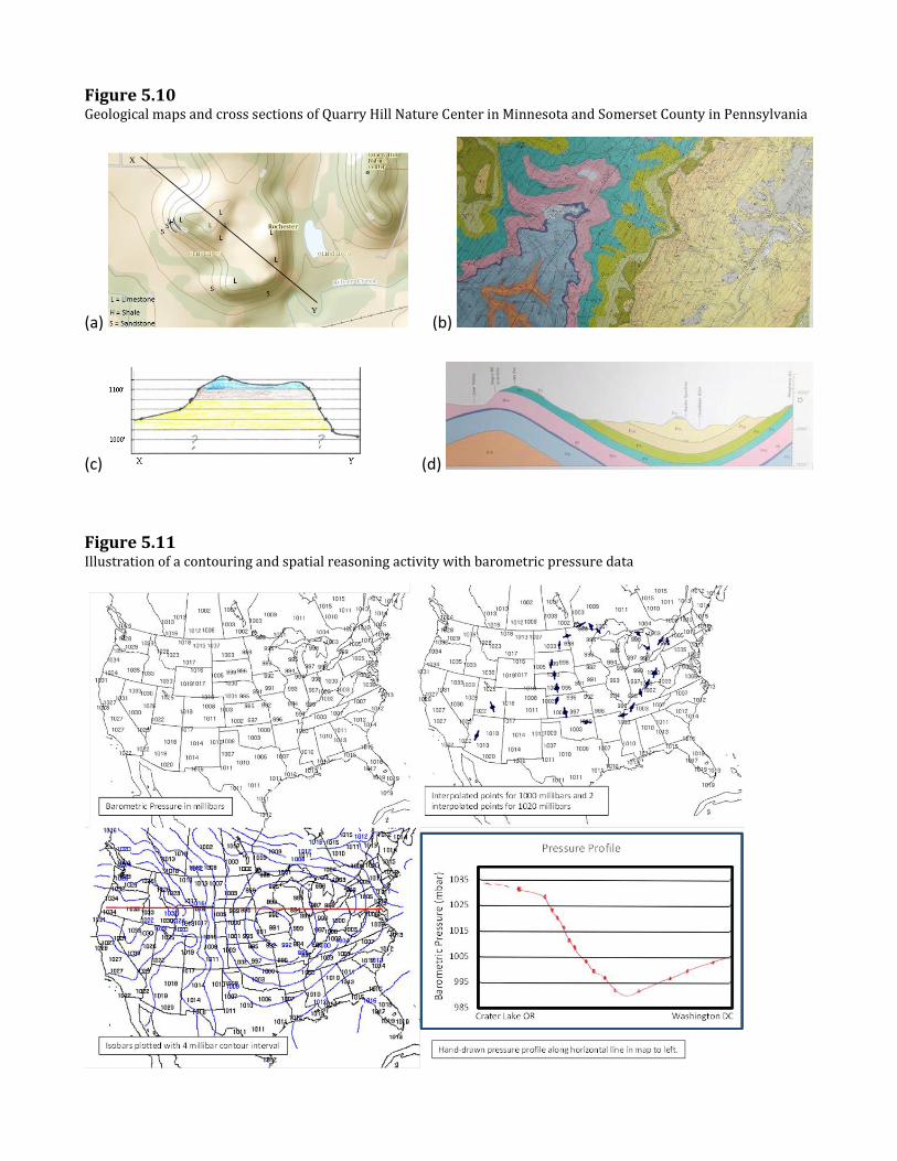
Figure 5.10Geological maps and cross sections of Quarry Hill Nature Center in Minnesota and Somerset County in Pennsylvania

(a) (b)

(c) (d)

Figure 5.11 Illustration of a contouring and spatial reasoning activity with barometric pressure data

Y

X

1000'

1100'

Y X

Figure 6.3A simple classroom barometer

Figure 6.7 Modification of a simple classroom barometer to improve performance

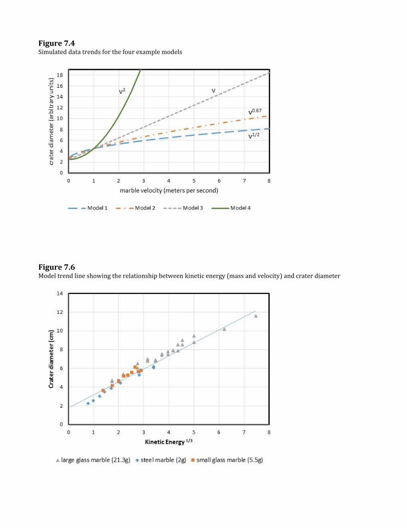
Figure 7.4Simulated data trends for the four example models

Figure 7.6Model trend line showing the relationship between kinetic energy (mass and velocity) and crater diameter

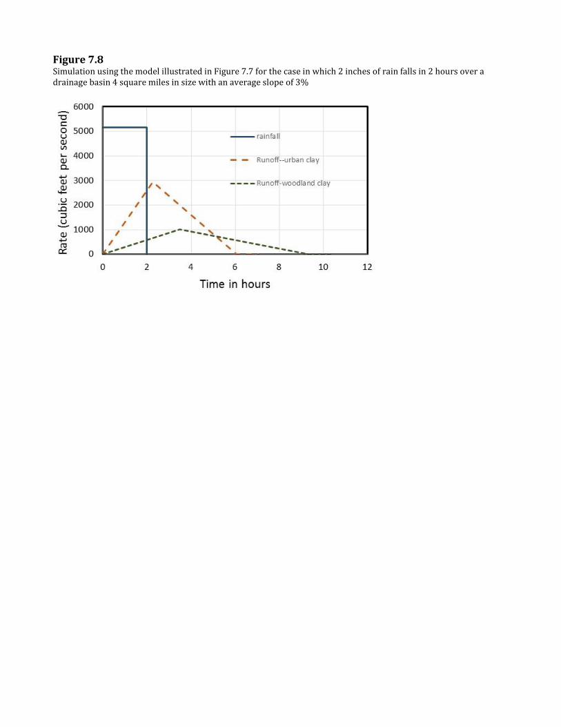
Figure 7.8Simulation using the model illustrated in Figure 7.7 for the case in which 2 inches of rain falls in 2 hours over a drainage basin 4 square miles in size with an average slope of 3%

Figure 10.1Rocks and images for the Edmontosaurus activity

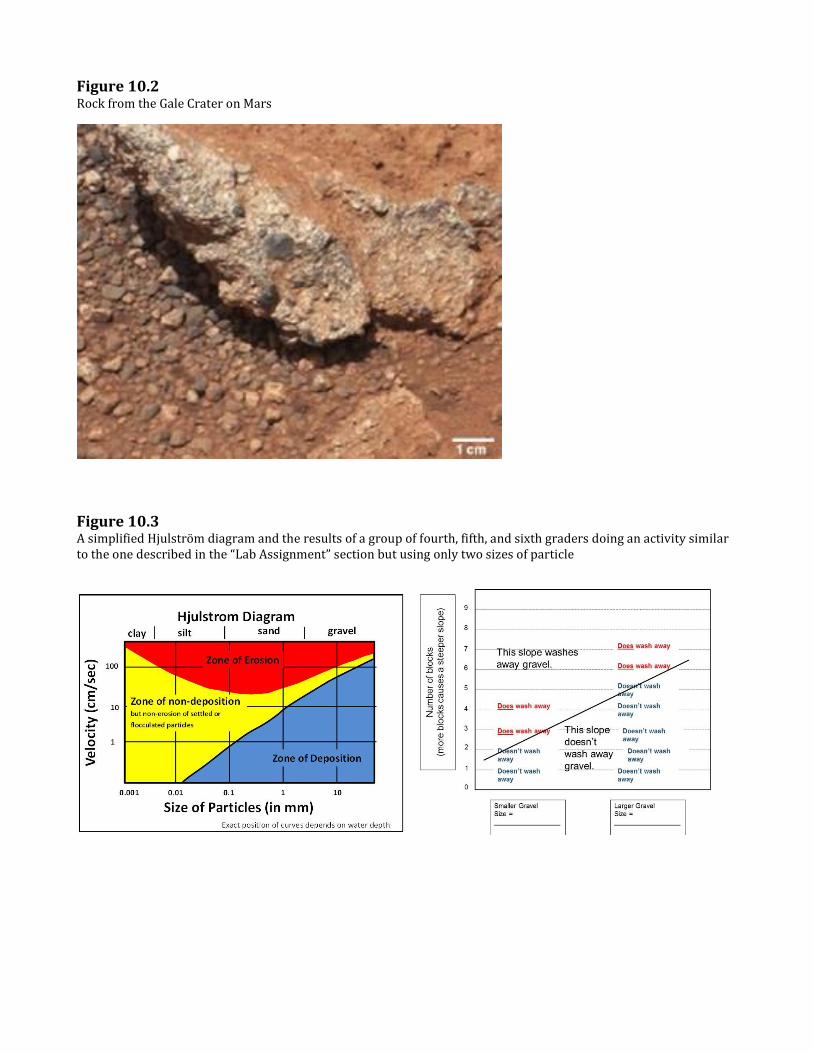
Figure 10.2Rock from the Gale Crater on Mars

Figure 10.3A simplified Hjulström diagram and the results of a group of fourth, fifth, and sixth graders doing an activity similar to the one described in the “Lab Assignment” section but using only two sizes of particle

Figure 11.3Science reasoning challenge for Powell’s unit A rocks in the Grand Canyon

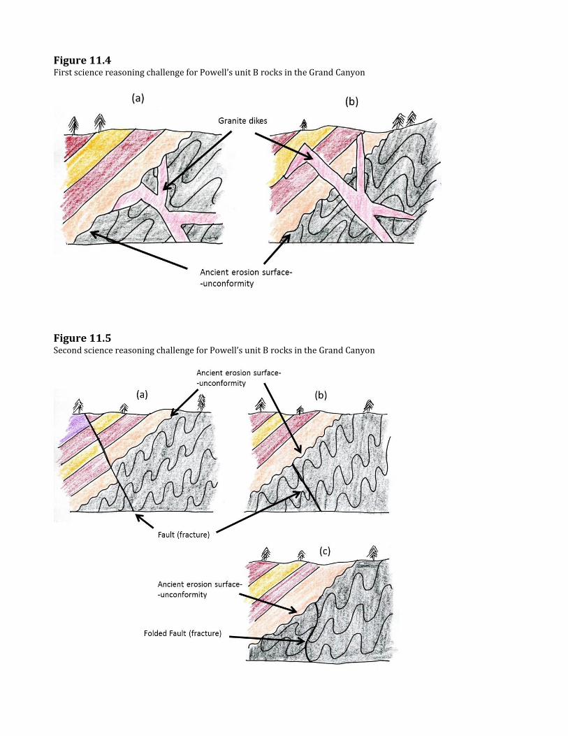
Figure 11.4First science reasoning challenge for Powell’s unit B rocks in the Grand Canyon

Figure 11.5Second science reasoning challenge for Powell’s unit B rocks in the Grand Canyon

Figure 11.7Modern cross-section illustration of the rocks at the Grand Canyon showing the relationship to Powell’s units A, B, and C

Figure 11.8Pattern of sediment off the East Coast of the United States

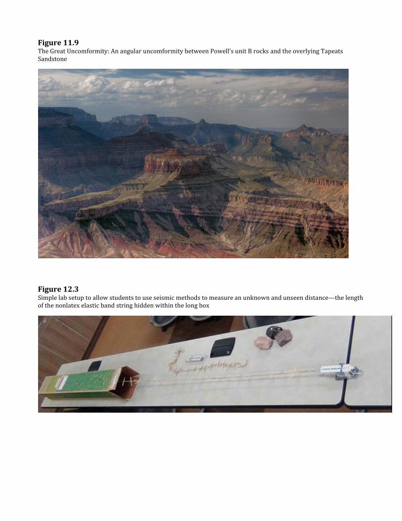
Figure 11.9 The Great Uncomformity: An angular uncomformity between Powell’s unit B rocks and the overlying Tapeats Sandstone

Figure 12.3Simple lab setup to allow students to use seismic methods to measure an unknown and unseen distance—the length of the nonlatex elastic band string hidden within the long box

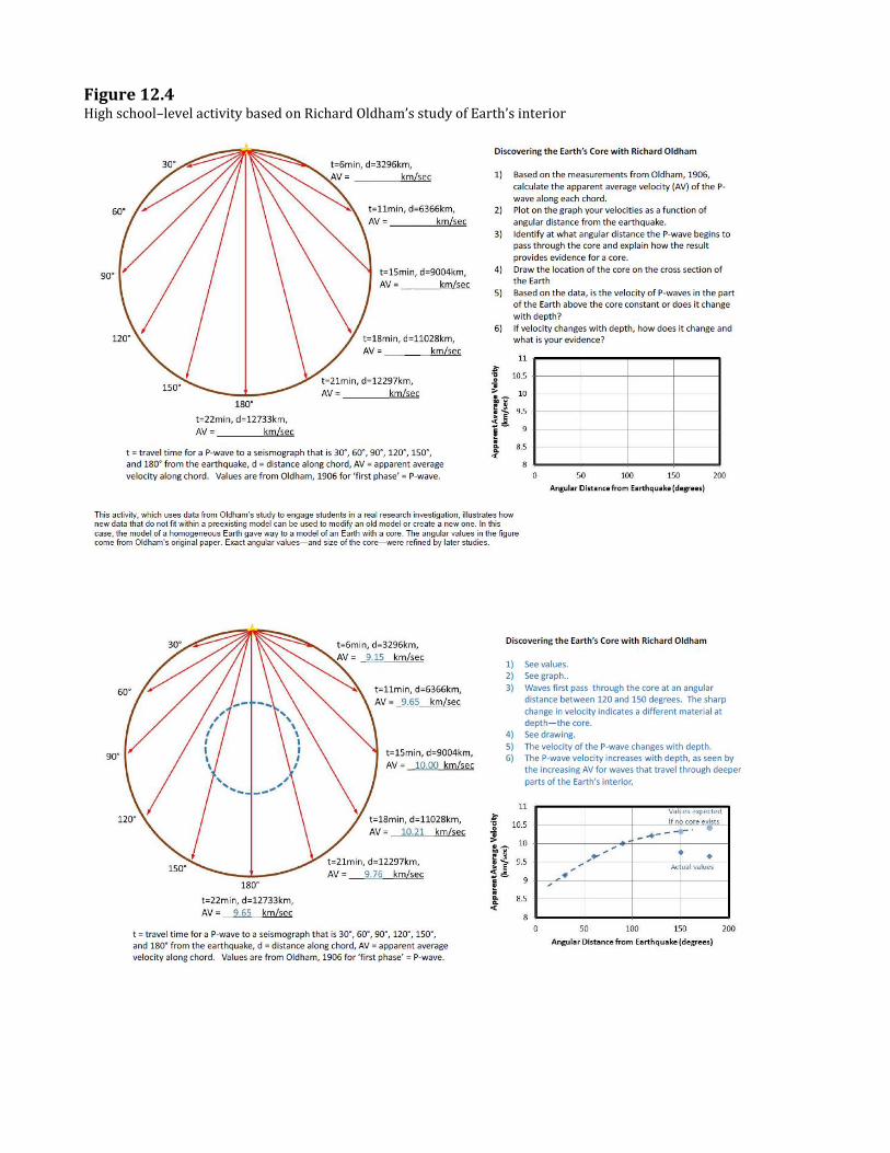
Figure 12.4 High school–level activity based on Richard Oldham’s study of Earth’s interior

Figure 12.5Illustration of the P- and S-wave shadow zones where P and S waves do not show up at seismic stations on the opposite side of the Earth from an earthquake

Figure 13.1Common illustration of the phases of the Moon, as viewed from above the Earth’s North Pole (sizes and distances of bodies are not to scale)

Figure 13.3Illustration of a model for the phases of the Moon, showing the time of day at different locations on the Earth (e.g., midnight on the side of Earth away from the Sun and noon on the side of the Earth toward the Sun) (sizes and distances of bodies are not to scale)

Figure 13.4Illustration of a common misconception of the Ptolemaic (Earth-centered) model of the solar system, with only the Earth, Sun, Venus, and the Moon shown (sizes and distances of bodies are not to scale)

Figure 13.5Illustration of the Ptolemaic model of the solar system, showing only the Earth, Sun, Venus, and Moon (sizes and distances of bodies are not to scale)

Figure 13.6Simplified illustration of the Copernican (Suncentered) model of the solar system, showing the Earth, Sun, Venus, and Moon (sizes and distances of bodies are not to scale)

Figure 13.9Model of the concept behind spectroscopy

Figure 13.10Example spectroscopy puzzle 1

Figure 13.11Example spectroscopy puzzle 2

Figure 13.12Using measurements and trigonometry to determine the angle between the Moon and the Sun

½ DH/AL

ASIN (½ DH/AL)

Figure 13.13Example observational data record from which a lunar phase model can be constructed

Figure 14.1Illustration of a modeling puzzle in geochemical evolution

Figure 14.2Illustration of a modeling puzzle in geochemical evolution similar to that in Figure 14.1, but starting with a different magma composition

Figure 14.6Two experiments with two different kinds of sediment that address the question of whether the spilled pesticide will get into Grandma’s well

Figure 14.7Manufacture of a set of standards by which the composition of water samples from the Grandma’s well experiments can be measured

Figure 14.8Illustration of the use of standards to analyze the concentration of red food coloring in the experimental water samples for the Grandma’s well experiments

Figure 14.9Simplified version of Grandma’s well experiment from Figure 14.6 for younger students or shorter duration

Figure 14.10Model of a magmatic process and a hydrothermal process to concentrate gold

Figure 15.4Illustration of the nested relationship among the three NGSS earth science DCIs, with superimposed big ideas

Figure 16.1Delta feature in a farm field associated with a storm that hit northwestern Minnesota in June 2000, showing the relationships that were necessary to figure out before developing the question-asking game

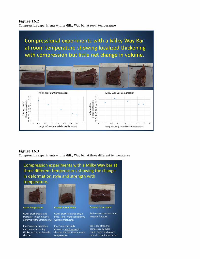
Figure 16.2Compression experiments with a Milky Way bar at room temperature

Figure 16.3Compression experiments with a Milky Way bar at three different temperatures