fuel composition and quality sensing for diesel engines …
TRANSCRIPT

FUEL COMPOSITION AND QUALITY SENSING FOR DIESEL ENGINES
BY
JOHN CLINTON SCHEIDER
THESIS
Submitted in partial fulfillment of the requirements
for the degree of Master of Science in Mechanical Engineering
in the Graduate College of the
University of Illinois at Urbana-Champaign, 2011
Urbana, Illinois
Adviser:
Professor Alan Hansen

ii
ABSTRACT
The range of fuels that a diesel engine may be expected to burn is increasing including
the use of biodiesels and alcohols produced from various plant or animal sources. Moreover,
fuels can become unsuitable for application in diesel engines due to a variety of contamination,
degradation, and cold flow issues. In order to optimize engine performance and meet EPA
emissions standards over a wide array of fuels, information about the fuel composition must be
known in real time. Furthermore, protecting the engine from potential fuel contaminants such as
water, sulfur, glycerol, methanol, and urea requires a method of detecting these chemicals in the
fuel system. This study evaluates a commercially available fluid properties sensor for use in
diesel engines. The sensor provides four bulk outputs: temperature, density, dynamic viscosity,
and dielectric constant, which can be used to monitor fuel properties.
Extensive testing was carried out on the sensor to evaluate its effectiveness at detecting
fuel type, blend, and quality over a temperature range of 0°-80°C. Fuel types tested include
diesel #1, diesel #2, jet A, soy biodiesel, rapeseed biodiesel, false flax biodiesel, jatropha
biodiesel, soy oil, rapeseed oil, false flax oil, and jatropha oil. Blends of diesel #1 and #2 with
soy biodiesel were studied. Fuel properties under contamination and the sensor’s sensitivity to
fuel degradation and cold flow situations were examined. A predictive model of fuel properties
was developed based on fuel composition, contamination, and temperature range. Finally, an
algorithm was developed to predict fuel type, blend, contamination condition, and degradation
condition for unknown fuel samples.

iii
ACKNOWLEDGEMENTS
Financial support for this work was provided through the John Deere Technology and
Innovation Center located in Champaign, Illinois.
Many have contributed to this project, and I would like to extend thanks to Dr. Alan
Hansen who has advised me and guided me through both the technical details of this project and
the process of completing my degree. He has been an invaluable part of my success as a student
and an engineer.
Furthermore, I must convey gratitude to the other members of my review committee: Dr.
Mary-Grace Danao of the Department of Agricultural and Biological Engineering and Dr.
Dimitrios Kyritsis of the Mechanical Science and Engineering Department.
Moreover, I would like to express appreciation for the help I have received from John
Deere. Especially Jim Lenz, director of JDTIC, for connecting me with this project, and Bruce
Upchurch, Sensor Development Engineer for John Deere Power Systems, for his advice and
technical support. Without their help this project would not have had proper direction. Also,
thanks to Ken Chao of John Deere Power Systems for his help in obtaining the fuel samples used
in this study.
Finally, thanks to my family and friends who have taught me the value of education.

iv
TABLE OF CONTENTS
LIST OF ABBREVIATIONS .........................................................................................vii
CHAPTER 1: INTRODUCTION .................................................................................... 1
CHAPTER 2: OBJECTIVES ........................................................................................... 4
CHAPTER 3: REVIEW OF LITERATURE .............................................................. 6
3.1 Fuel Properties ................................................................................................................. 6
3.2 Variation of Properties with Temperature .................................................................... 8
3.2.1 Viscosity ..................................................................................................................... 8
3.2.2 Density ..................................................................................................................... 10
3.2.3 Dielectric Constant .................................................................................................. 12
3.2.4 Cold Flow ................................................................................................................ 13
3.3 Variation of Properties with Fuel Composition or Blend ............................................. 15
3.3.1 Comparison of Petroleum-based Diesel and Biodiesel ........................................... 15
3.3.2 Blends of Fuels ......................................................................................................... 19
3.3.3 Biodiesel from Different Sources ........................................................................... 22
3.3.4 Vegetable Oil Composition ..................................................................................... 25
3.4 Effect of Contaminants on Fuel Properties ................................................................... 27
3.4.1 Water ....................................................................................................................... 27
3.4.2 Sulfur ....................................................................................................................... 31
3.4.3 Glycerol ................................................................................................................... 32
3.4.4 Alcohol .................................................................................................................... 34
3.5 Effect of Time or Degradation on Fuel Properties ....................................................... 35
3.6 Sensors for Detection of Fuel Composition ................................................................... 37
3.6.1 Resonant Cavity Dielectric Sensors ........................................................................ 38
3.6.2 Spectroscopic Techniques ....................................................................................... 39
3.6.3 Microelectromechanical Systems ............................................................................ 42
CHAPTER 4: MATERIALS AND METHODS ....................................................... 43
4.1 Sensor Operation ........................................................................................................... 43
4.2 Fuel Acquisition and Preparation ................................................................................. 45
4.3 Fuel Type Property Measurement ................................................................................ 49
4.4 Fuel Blend Property Measurement ............................................................................... 50
4.5 Fuel Contamination Experimentation .......................................................................... 51

v
4.6 Fuel Degradation Experimentation .............................................................................. 55
4.7 Development of a Classification Model ........................................................................ 57
4.7.1 Algorithm Format .................................................................................................. 57
4.7.2 Regression Models for Fuel Properties .................................................................. 57
4.7.3 Sensitivity and Limits of Regression Models ......................................................... 58
4.7.4 Sensor Outputs to Identify Contamination or Degradation ................................. 61
4.7.5 Neural Networks for Fuel Classification ................................................................ 63
CHAPTER 5: RESULTS AND DISCUSSION ......................................................... 65
5.1 Fuel Type Properties Measurement ............................................................................. 65
5.1.1 Sensor Output for Petroleum Based Fuels and Biodiesel ..................................... 65
5.1.2 Measurement of Diesel Fuels with Different Sulfur Content ................................ 69
5.1.3 Sensor Outputs for Biodiesels from Different Oil Sources ................................... 71
5.1.4 Property Measurement of Plant Oils ..................................................................... 76
5.1.5 Summary of Results ............................................................................................... 79
5.2 Fuel Blend Properties Measurement ............................................................................. 80
5.2.1 SME Biodiesel Blends with Diesel #2 ..................................................................... 80
5.2.2 SME Biodiesel Blends with Diesel #1 ...................................................................... 83
5.2.3 Summary of Results ............................................................................................... 86
5.3 Effect of Fuel Contamination on Sensor Outputs ........................................................ 86
5.3.1 Water ...................................................................................................................... 87
5.3.2 Sulfur ...................................................................................................................... 96
5.3.3 Urea ......................................................................................................................... 98
5.3.4 Glycerol ................................................................................................................. 102
5.3.5 Methanol ............................................................................................................... 108
5.3.6 Summary of Results ............................................................................................. 111
5.4 Effect of Fuel Degradation on Sensor Outputs .......................................................... 112
5.5 Development of a Fuel Classification Model .............................................................. 118
5.5.1 Algorithm Format ................................................................................................ 118
5.5.2 Regression Models for Fuel Properties with Temperature ................................. 120
5.5.3 Regression Models for Fuel Properties with Blend ............................................. 123
5.5.4 Sensitivity and Limits of Regression Models ....................................................... 126
5.5.5 Identification of Contaminants or Degradation ................................................... 129
5.5.6 Neural Network to Identify Fuel Composition and Contamination .................... 132
5.5.7 Summary of Results .............................................................................................. 137

vi
CHAPTER 6: SUMMARY AND CONCLUSIONS .............................................. 139
CHAPTER 7: RECOMMENDATIONS FOR FUTURE WORK .................... 143
REFERENCES ................................................................................................................ 144
APPENDIX A: 3-D PLOTS OF SENSOR OUTPUTS ......................................... 147
APPENDIX B: PLOTS OF CONTAMINATION EFFECTS ........................... 152

vii
LIST OF ABBREVIATIONS
ASTM American Society of Testing and Materials
B-x Blend of biodiesel with petroleum based diesel (#2 unless otherwise stated) where
x = % biodiesel by volume
DEF Diesel Exhaust Fluid
DPF Diesel Particulate Filter
EPA Environmental Protection Agency
E-x Blend of ethanol with gasoline where x = % ethanol by volume
FAME Fatty Acid Methyl Ester
GUI Graphical User Interface
MEAS Measurement Specialties Company
PPM Parts Per Million: the concentration of a substance within a solution usually on a
volume basis
RME Rapeseed Methyl Ester
SCR Selective Catalyst Reduction
SME Soybean Methyl Ester
ULSD Ultra Low Sulfur Diesel Fuel

1
CHAPTER 1: INTRODUCTION
Diesel engines are proven, effective power producers for a number of uses across the
transportation and stationary power generation industries. While primarily run on petroleum
based diesel fuel, diesel engines have been successfully operated with a number of different fuels
and oils. In particular, there has been great interest in running engines on biodiesel and even
vegetable oils or blends of these with traditional petroleum fuels due to the positive emissions
and environmental consequences of using bio-based fuel sources. Engines can often use
biodiesel or vegetable oils without any modification to the engine’s physical design or controls;
however, much research has been dedicated to the combustion of such fuels and their blends and
improving performance and emissions as a function of engine controls, injection timing and rate,
exhaust gas recirculation (EGR), or exhaust after-treatment. Controls optimization requires real
time information about fuel composition that can be supplied to the engine controls unit. While
there are systems currently in place to determine fuel composition in spark ignition engine
applications, there exists no such complete sensing system available for use specifically in diesel
engines, although several available sensor types may be suitable for such a function (Tat and Van
Gerpen, 2003b).
In addition to the need for engines to be flexible in their use of fuels, fuels need to be
clean and of high quality in order to assure proper engine function. The refining industry takes
great care to provide fuels that meet these standards for fuel quality; however, several conditions
can render fuel inappropriate for engine use. First, water can mix with fuels due to leaks in tanks
and seals or from condensation. Contamination from water can damage fuel pumps, filters, and
injectors as well as affecting the combustion process. Secondly, sulfur is present in all petroleum
based fuels and its content is highly regulated. Studies show that high sulfur fuels very quickly

2
destroy the efficiency and life of many after-treatment systems such as diesel particulate filters.
Third, biodiesel is susceptible to contamination from both methanol, which is a reactant in the
biodiesel production reaction, and its byproduct glycerol. Biodiesel quality standards require
that these components be controlled to a low concentration (ASTM, 2010a). Finally, there are
many other potential contaminants of diesel fuels including gasoline and urea based diesel
exhaust fluid.
Another potential problem is fuel degradation; fuels occasionally sit in storage within a
machine or storage tank for long periods of time and age to the point of causing unsatisfactory
engine operation. Bio-fuels have higher viscosities and cloud points which often lead to starting
and fuel flow problems for engine users in cold climates (Joshi and Pegg, 2007). Ultimately
there are a number of problems that can arise to make fuels less than ideal for engine use, and
engine manufacturers have begun to recognize the value of protecting their customers from
improper or contaminated fuels.
This study focuses on the development and application of fuel composition and quality
sensors for use on diesel engines. The sensor used in this study is a commercially available fluid
properties sensor developed and manufactured by Measurement Specialties (MEAS), (Model no.
FPS 2800). This sensor provides four bulk fluid properties as its outputs: dynamic viscosity,
density, dielectric constant, and temperature. Analysis of fluid properties could be used to
supply real time information about fuel composition and quality to the engine control unit or the
operator station. Such information would be useful in optimizing engine performance and
protecting the engine through the use of warning signals pertaining to the suitability of the fuel
for the application.

3
In order to employ the sensor for engine controls and diagnostic warnings, information of
importance such as fuel type, blend, presence of contaminant, contamination level, type of
contamination, degradation condition, or cold flow problem was extracted from the outputs of
the sensor and modeled over a wide range of fuels (both petroleum and bio based) over the
applicable temperature range. Also, blends of diesel and biodiesel fuels were examined. Sensor
response to contamination by water, sulfur, glycerol, methanol, and urea as well as degraded fuel
was studied. An in-depth understanding of the effect of composition and temperature on each
sensor output was necessary. Models of the MEAS sensor’s response were compiled to yield an
algorithm capable of predicting the fuel type, blend, presence and level of contamination,
degradation, and cold flow problems in an unknown fuel sample.
In the following chapters the objectives of this study are more precisely stated (Chapter
2), and a literature review of fuel quality sensing, fuel properties, temperature effects on fluid
properties, composition/blending effects on fluid properties, and engine performance related to
fuel type and quality is compiled and summarized (Chapter 3). A detailed description of the
experimental methods and procedures is presented (Chapter 4). Finally, the conclusions of this
study (Chapter 5), in addition to recommendations for future work sum up the content of this
thesis (Chapters 6 and 7).

4
CHAPTER 2: OBJECTIVES
The overall goal of this project was to develop a fuel quality sensing system capable of
providing information that could be used for either engine controls or warning signals that would
add value to engine product lines. Within the scope of that goal there were a number of specific
objectives that were realized related to both implementation of sensors and the science of fuels.
1. MEAS sensor outputs (dynamic viscosity, density, dielectric constant) were calibrated for
diesel #1, diesel #2, SME B-100, and JET A, fuels over a temperature range of 0°-80° C.
2. MEAS sensor outputs (dynamic viscosity, density, dielectric constant) were calibrated for
blends of SME biodiesel with diesel #2 in 10% vol. increments over the temperature
range of 20°to 80° C. Also, calibration of outputs for blends of diesel #1 with SME
biodiesel for blends up to 20% vol. of SME was conducted.
3. The effect on dynamic viscosity, density, and dielectric constant from contamination of
diesel #2 and several blended fuels by water and urea were determined as well as
contamination of B-100 by glycerol and methanol. Sulfur contamination was studied in
diesel #2 only.
4. The effect storage time has on the degradation of fuels with respect to changes in
dynamic viscosity, density, and dielectric constant was determined.
5. The properties of biodiesel from different sources such as soybean, rapeseed, jatropha,
and false flax on viscosity, density, and dielectric constant were evaluated. These
differences were related to the measured fatty acid profiles of each biodiesel.

5
6. MEAS sensor data were compiled and used to develop an algorithm capable of using the
sensor outputs to provide the base fuel type, level of blend with biodiesel, level of
contamination, type of contamination, level of degradation, and indication of cold flow
problems.
7. Recommendations for the implementation of the sensor in engine applications were
provided.

6
CHAPTER 3: REVIEW OF LITERATURE
In order to serve the primary objectives of this project which were application based and
focused on delivering functional engineering results, it was necessary to understand the subject
of fuel sensing on a deeper level. Knowledge of the properties of fuels and previous work on
fuel sensing allowed this project to be grounded in firm science. This literature review will
cover some of the extensive research that has previously been attempted within the following
topics:
• Properties of fuel: Variation of these properties with temperature and composition,
• Fuel contaminants,
• Stability and degradation of fuels, and
• Sensors for detection of fuel or fluid properties.
3.1 Fuel Properties
When attempting to identify or distinguish different substances or blends it is necessary
to have a measurement or set of measurements that can be used as a determinant between the
possible inputs. In the case of a liquid such as fuel there are two obvious routes for
measurement. The first is to identify the specific chemical composition of the liquid providing
the definite ratios of elements or molecules. Spectroscopic techniques provide this level of
specificity and sensitivity giving a very accurate analysis of the composition and therefore
identification of a material. However, in an application such as real time fuel sensing in engines
this type of sensor is often either too expensive or incapable of providing fast results.
Alternatively, a measure of the bulk properties of liquids and their blends could be used. In the
case of fuels there were several possible bulk properties that might be chosen for measurement in

7
the application of fuel sensing. Some potential properties could be identified from inspection of
ASTM standard D975 such as: density or specific gravity, kinematic viscosity, volatility, colour,
corrosivity, and lubricity (ASTM, 2010b). In addition other properties beyond those of typical
interest within fuels standards could be identified including dielectric constant, dynamic
viscosity, electrical resistivity, pH, or surface tension.
In theory, any of these properties is a potential determinant for a fuel sensing system. In
practice however, the property must be easily measured in a very short time period. Therefore
properties such as corrosivity and lubricity are not practical. Another criterion in determining
the best properties to measure is the difference between the values of the property at each end of
the range of fuels of interest. For example, to measure the blend level of biodiesel with #2 diesel
a property that has a very different value for each of the two neat fuels is optimal.
There is a dearth of fuel properties for different types of biofuels and their bends. In
some cases there were discrepancies between measured values and their sampling conditions,
making direct comparisons difficult to achieve. For the range of fuels used in this study, both
kinematic viscosity and dielectric constant vary greatly across fuel type (Table 3.1)
Table 3.1 Selected fuel properties (Dubovkin and Malanicheva, 1981; Graboski and
McCormick, 1998; Tat and Van Gerpen, 2003; Yuan, 2005)
Fuel Kinematic viscosity (cSt)a
Density (g/ml)b
Dielectric Constant
Diesel #1 1.7590 0.8162 2.0800
Diesel #2 2.6000 0.8537 2.1000
Jet A 1.1300 0.7895 1.7000
Gasoline 0.7000 0.7450 2.0000
SME B-100 4.0800 0.8853 ~3.2
RME B-100 4.8300 0.8820 NA a Measured at 40°C b Measured at 20°C

8
It can be seen that kinematic viscosity and dielectric constant could be potential
properties for distinguishing between fuel types while density would be useful to a lesser level.
While several of the other properties previously listed have potential for application to fuels
sensing, the MEAS sensor employed in this study utilizes measurement of the dynamic viscosity,
density, and dielectric constant. Consequently these will be the properties of focus for the
remainder of this literature review.
It should be noted that the MEAS sensor provided dynamic viscosity rather than
kinematic viscosity. However, dynamic viscosity is merely the kinematic viscosity divided by
the density, and the density was essentially constant in comparison to viscosity in most cases.
Therefore any trends that hold for kinematic viscosity also held for the dynamic viscosity in
general. This was fortunate since nearly all data available are for kinematic viscosity rather than
dynamic viscosity.
3.2 Variation of Properties with Temperature
Practically all bulk properties of liquids have some dependence on temperature; therefore,
in order to develop a highly accurate system of fuel composition sensing it was necessary to
understand this temperature dependence for each sensor output. This section focuses on each of
the three properties the MEAS sensor monitors and their relationship to temperature.
3.2.1 Viscosity
It was well documented within the literature that the temperature dependence of liquid
kinematic viscosities was a very strong function with a non-linear shape. However, there had
been a long history of attempts to accurately describe this relationship.

9
The most basic model was an exponential model which works over limited temperature
ranges.
���� = ��exp �−��� (3.1)
where T is the temperature η is the kinematic viscosity, and η0 and b are constant coefficients.
(Seeton, 2006)
A more fundamental model was the Arrhenius model based on the Arrhenius equation for
molecular kinetics.
���� = ��exp ���� (3.2)
where η0 is a constant coefficient, T is the temperature, E is the activation energy, and R is the
universal gas constant (8.3415 J K-1
mol-1
). (Seeton, 2006)
Indeed many other empirical relationships had been used to accurately describe the
viscosity-temperature relationship. Seeton (2006) compiled several more of these relationships.
Valeri and Meirelles (1997) applied the Andrade correlation and its modified versions to
model the temperature dependence of several fatty acids and triglycerides with high success.
Their model produced mean deviations of less than 2.5% over a temperature range of 20°-90°C:
ln � = � + �/� (3.3)
where η is the kinematic viscosity (cSt) A, and B are empirical constants and T is the temperature
(°C)
Although there have been few attempts to characterize the viscosity- temperature
correlation specifically for fuel Tat and Van Gerpen (1999) utilized a form of the modified
Andrade Correlation as described above to model the temperature relationship for viscosities of

10
blends of diesel #2 and biodiesel. Their model was accurate over a temperature range of -20° to
100°C for the entire range of blends.
Modified Andrade Correlation:
ln � = � + �� + �
�� (3.4)
where η is the kinematic viscosity (cSt), T is the temperature in Celsius and, A, B, and C are
empirical constant coefficients determined from data (Tat and Van Gerpen, 1999)
3.2.2 Density
Density in fuels has been a subject of research due to its importance in the control of the
mass of fuel injected in high pressure diesel injection systems. However, within this work the
temperature dependence of density had been established and may be applied to a fuel sensing
application. The dependence of density on temperature was known to be much less dramatic
than that of viscosity and to be of nearly linear shape. As such density was much easier to model
over wide temperature ranges for most liquids including fuels.
Most authors suggested that density can be simply modeled with temperature using a
linear model of form:
� = � − �� (3.5)
Where ρ is the density (g/ml), t is the temperature in Celsius, and b and m are regression
coefficients
Fischer (1995) attempted to summarize and organize previous attempts of modeling fatty
acid temperature relations. His study yielded results for a wide range of compounds using the
above linear form with the coefficients for the model displayed in Table 3.2.

11
Table 3.2 Linear density temperature dependence coefficient constants for fatty acids
(Fischer, 1995)
Fatty Acid Intercept b (g/ml) Slope m (g/ml/°C)
C9:0 0.92106 7.923E-04
C10:0 0.91660 7.824E-04
C12:0 0.90813 7.486E-04
C14:0 0.90274 7.269E-04
C16:0 0.89809 7.083E-04
C18:0 0.89535 6.974E-04
Tat and Van Gerpen (2000) applied a similar linear model to fuels including diesel #1,
diesel #2, SME B-100, B-75, B-50, and B-20. They also compared their results for biodiesel and
blends to the established guidelines from ASTM standard D1250 which provides tables for
temperature correction of density measurements for diesel fuels. These tables were established
to allow engineers to measure fuel density at any temperature and then correct their findings to a
common standard temperature for comparison. The study found that the same linear model was
appropriate for biodiesel and its blends, and that ASTM D1250 tables could be used for any of
these fuels. This suggested the rate of change of density with temperature was independent of
fuel blending with biodiesel. In addition the accuracy of their models was apparent in the R2
values of the regressions provided which were all above .998 (Table 3.3).

12
Table 3.3 Regression coefficients and errors for linear models of fuel density temperature
dependence (Tat and Van Gerpen, 2000)
Fuel Type Intercept a Slope b R2
MSD
Blends with #2 Diesel
B-100 0.8976 -6.62E-04 0.9989 4.830E-07
B-75 0.8869 -6.80E-04 0.9997 1.200E-07
B-50 0.8750 -6.71E-04 0.9994 3.138E-07
B-20 0.8613 -6.60E-04 0.9989 6.211E-07
Diesel #2 0.8527 -6.41E-04 0.9989 5.969E-07
Blends with #1 Diesel
B-75 0.8831 -6.82E-04 0.9995 2.654E-07
B-50 0.8678 -6.70E-04 0.9995 2.368E-07
B-20 0.8506 -6.61E-04 0.9995 3.024E-07
Diesel #1 0.8403 -6.63E-04 0.9994 3.548E-07
3.2.3 Dielectric Constant
A general model of the dielectric constant developed from the geometry of the basic
molecules or atoms of the substance is an achievement not yet fully realized. Fortunately there is
a great deal known about the dielectric constant of liquids and temperature although this theory
had not been widely applied to fuels. The study of dielectric constant has to be broken up into
two regimes: polar liquids and non-polar liquids. The behavior of these two types of liquids is
quite different. Moreover, the ability of polar molecules to align themselves with the electric
field is the primary cause for the much higher dielectric constants of such materials. Also, the
temperature dependence of dielectric constant is different in each of the two cases. In general
within the liquid phase polar molecules have a much higher rate of change of dielectric constant
with temperature compared to non-polar liquids. Non-polar liquids were of higher interest since
fuels fall within this category. However, polar liquids were of some interest as well since water
is highly polar and is one of the main fuel contaminants to be addressed in later sections.

13
Non-polar liquids such as fuel have dielectric properties that are largely insensitive to
temperature change although the dielectric constant will decrease slightly as temperature
increases.
Sen et al. (1992) found that the static dielectric constants of many hydrocarbons decrease
linearly with temperature over a range of 100-300 K within which the alkanes were liquid. Sen
et al (1992) were able to explain these results through use of an established model. Furthermore,
it was found that the dielectric constant was actually dependent on the density of the liquid. The
number of molecules available to store energy within the electric field will decrease as density
decreases causing the subsequent decline in dielectric constant. Succinctly, dielectric constant
was inversely linearly proportional to temperature since density was inversely linearly
proportional to temperature and is best described by the Clausius- Mosotti Relation:
�� !"#�� $%� = 4'�()
*+, (3.6)
where ε’ is the dielectric constant, ρ is the density, Na is Avogadro’s number, α is the electric
polarizability of the molecule, and M is the molecular weight of the liquid (Sen et al., 1992).
Comparisons of measurement to this model produced less than 0.3% error above 0°C and
less than 1% error below 0°C.
3.2.4 Cold Flow
The trends of fuel properties described above are relevant for the liquid form of the fuel
in temperature ranges approximately near standard conditions above 0°C. Consequently, as fuels
are cooled to near the phase transition point to a solid these models would no longer be accurate.
When developing algorithms based on measurements taken with a fluid properties sensor the

14
lower limit of application of these prediction formulae was near the cloud point of the fuel, the
temperature at which the fuel begins to cloud or show evidence of crystal formation.
Fortunately, research has been conducted to quantify the cloud point for diesel fuels and
blends with biodiesel. Joshi and Pegg (2007) measured the cloud points of diesel #2 and blends
with biodiesel made from fish oil, and fitted a model to relate cloud point to blend level. The
model was a quadratic polynomial of the form shown in equation 3.7. Also, Table 3.4 includes
results from this model and experimentation.
�-. = 256.4 + .1991 5� + .0002235�% (3.7)
Tcp refers to the cloud point temperature in Kelvin, and VB is the blend percentage by volume.
Table 3.4 Cloud points of blends of diesel #2 and biodiesel from fish oil (Joshi and Pegg,
2007)
Blend Cloud Point (K) Cloud Point °C Predicted Cloud Point (K)
B100 279 6 278.6
B80 273 0 273.8
B60 269 -4 269.2
B40 265 -8 264.7
B20 261 -12 260.5
B0 256 -17 256.4
The model and measurements agree that the cloud point of diesel #2 was much lower
than that of biodiesel. Moreover, considering normal temperatures in the US, diesel #2 would
almost never be cooled to its cloud point but pure biodiesel would often be colder than its cloud
point in winter seasons. The model presented predicted cloud point with high accuracy;
however, as can be seen by the small coefficient on the quadratic term this relationship was
nearly linear suggesting a simpler model would also be successful.

15
Other studies indicated that cloud point could vary significantly based on the fatty acid
composition of the biodiesel. Imahara et al. (2006) measured the cloud points of several
biodiesel samples in order to verify a model developed to predict cloud point based on fatty acid
composition (Table 3.5)
Table 3.5 Cloud points of biodiesel (Imahara et al., 2006)
Biodiesel Cloud point (K)
Linseed 268
Safflower 267
Sunflower 274
Rapeseed 267
Soybean 272
Olive 268
Palm 283
Beef tallow 286
3.3 Variation of Properties with Fuel Composition or Blend
The versatility of diesel engines with respect to the fuel they may combust places a
requirement on any reliable fuel sensing system that it be able to detect and distinguish between
a wide range of fuels. Consequently, a review of research related to how the chemical
composition of fuel affects its bulk properties was necessitated.
3.3.1 Comparison of Petroleum-Based Diesel and Biodiesel
The two most important sources of fuel for diesel engines are oil removed from the earth
and bio based oils harvested from various plant and animal sources. Moreover, a popular
strategy in North America and Europe is to use some combination of diesel fuels refined from
these two types of sources. Accordingly a successful fuel sensor had to be able to distinguish
between fuels from these two separate origins.

16
Again, the dynamic viscosity, density, and dielectric constant of these fuels and blends
must be examined. Viscosity and density for each type of fuel had been measured and compared
in several studies while discussion of the dielectric constant remained largely unavailable in fuel
literature.
Graboski and McCormick (1998) performed a detailed study on the properties of bio-
fuels in comparison with standard diesel fuels. Included within this work were some
measurements of the viscosity and density of diesel #2 and several biodiesels from different
sources. Also, Tat and Van Gerpen (1999, 2000, 2003) researched the density and viscosity of
diesel, biodiesel, and its blends over some temperature variation (Tables 3.6 through 3.9)
Table 3.6 Viscosity of several fuels (Graboski and McCormick, 1998)
Fuel Viscosity (cSt 40°C)
No. 2 Diesel Fuel 2.60
Soybean oil methylester 4.08
Rapeseed oil methylester 4.83
Tallow oil methylester 4.80
Soybean oil ethylester 4.41
Rapeseed oil ethylester 6.17
Palm oil methylester 4.50
Palm stearin methylester 4.60
Frying oil ethylester 5.78
Tallow ethylester 5.93
Tallow butylester 6.17

17
Table 3.7 Viscosity of several fuels (Tat and Van Gerpen, 2003)
Fuel Kinematic Viscosity (cSt 40°C)
No. 2 Diesel 2.8911
Soybean oil methylester 4.5926
Yellow Grease methylester 5.9156
Soybean oil isopropyl ester 5.2649
Yellow grease isopropyl ester 6.0997
Table 3.8 Specific gravity of several fuels at 20°C (Graboski and McCormick, 1998)
Fuel Specific Gravity
No. 2 Diesel Fuel .8500
Soybean oil methylester 0.8853
Rapeseed oil methylester 0.8820
Tallow oil methylester 0.8756
Soybean oil ethylester 0.8810
Rapeseed oil ethylester 0.8760
Sunflower oil methylester 0.8800
Cottonseed oil methylester 0.8800
Palm oil methylester 0.8700
Palm stearin methylester 0.8713
Frying oil ethylester 0.8716
Tallow ethylester 0.8710
Tallow butylester 0.8680

18
Table 3.9 Specific Gravity of several fuels (Tat and Van Gerpen, 2000)
Fuel Specific Gravity 20°C
#1 Diesel 0.8844
#2 Diesel 0.8399
Soybean oil methylester 0.8270
McCrady (2007) analyzed several types of biodiesel in his work on biodiesel property
definition for combustion modeling. Tables 3.10 and 3.11 show results for viscosity and density.
In general plant based biodiesels were more viscous than diesel #2 and percent increase in
density of plant-based fuels over diesel #2 ranged from 4 to 6%.
Table 3.10 Percent increase of viscosity of several biodiesels over diesel #2 (McCrady, 2007)
Percent Increase of Viscosity compared to #2 diesel
Temperature °C Soybean Rapeseed Coconut Palm Lard
20 58.0 84.0 30.5 65.9 81.2
40 65.1 84.8 34.2 87.8 75.6
60 75.0 92.3 36.1 89.5 83.8
80 75.4 89.7 37.3 83.5 80.0
100 60.4 72.9 30.7 75.1 68.3
Table 3.11 Percent increase of density of several biodiesels over diesel #2 (McCrady, 2007)
Percent Increase of Density compared to #2 diesel
Temperature °C Soybean Rapeseed Coconut Palm Lard
20 6.13 5.53 5.30 4.30 4.70
40 5.96 5.36 5.11 4.75 4.50
60 6.77 6.14 5.53 4.30 4.55
80 6.84 5.97 5.59 4.97 4.60
100 6.19 5.56 5.31 4.68 4.31

19
Unlike viscosity and density, dielectric constant had not been of interest to researchers in
the fuels and combustion area since this property seemed to have little effect on the ability of the
fuel system to pump and inject the fuel or the ability of the engine to perform combustion.
However for fuel sensing it was a very important and useful property to record.
One piece of research available looked at the feasibility of using the dielectric constant as
a fuel composition determinant. Tat and Van Gerpen (2003b) used a commercially available
dielectric flex fuel sensor similar to what Ford Motor Co. has used for on-board ethanol- gasoline
blending determination, for blends of diesel #1 or #2 and soybean biodiesel (Table 3.12). This
sensor measured changes in how the fluid responds to vibration and its output was a frequency
which was directly correlated with the dielectric constant.
Table 3.12 Dielectric resonance sensor response to different fuels (Tat and Van Gerpen,
2003b)
Fuel Sensor Output (frequency hz)
Diesel #1 51.84
Diesel #2 52.63
Soy methylester 58.96
3.3.2 Blends of Fuels
Standard petroleum-based diesel fuels are often blended with biodiesel in order to
maintain similar combustion or injection performance while taking advantage of some of the
advantages of biodiesel. A highly important variable that a diesel fuel sensing system in North
America could output is the blend percentage between diesel and biodiesel. Several studies have

20
reported the effects on density and viscosity but few ascertained the effects on dielectric
constant.
Density
Of the three properties of interest density is the easiest to model with changing fuel blend.
Since density is merely a measure of the amount of mass per unit volume this property changed
linearly when blending liquids.
Yang et al. (2004) studied 114 blends of diesel fuels as part of a study related to
developing a prediction system for the cetane number of these blends. Furthermore, as parts of
this work the density of the fuel was modeled using a mass weighting equation.
� = ∑ �9:" ;9 (3.8)
where ρ is the density, W is the mass fraction, and i denotes the ith component of the blend.
Tat and Van Gerpen (2000) applied this relationship to blends of diesel #1 or #2 with
SME biodiesel. The density of blends of these fuels was predicted with less than 0.3% error
from actual measurements.
McCrady (2007) confirmed the validity of this model with blends of #2 diesel and
soybean biodiesel, noting that the average percent increase of density over that of #2 diesel was
linear with the addition of biodiesel.
Viscosity
Compared to density the viscosity of blended fuels is more difficult to model over wide
temperature ranges because each component’s viscosity responds to temperature changes at
different rates.

21
Tat and Van Gerpen (1999) had studied the viscosity properties of blends in some detail.
Blends of diesel #1 or #2 with soy biodiesel were modeled with a correlation similar to the
Grunberg-Nissan equation.
ln �� = �" ln �" + �% ln �% (3.9)
where η is the viscosity, m is the mass fraction, and the subscripts refer to components or blend.
The inaccuracy of this model was less than 2% for all blends which was below the natural
deviation within the viscosity of fuel reported in the market. In addition it was noted that this
model was slightly more accurate for blends with #2 diesels attributable to the smaller ranges
between the viscosities of these two fuels in comparison to blends with #1 diesel.
McCrady (2007) used this model for blends of #2 diesel and soy biodiesel effectively.
This study observed the near exponential shape of the relationship between viscosity and blend
due to the use of the logarithm of each component in the correlation.
Dielectric Constant
Compared to density and viscosity, there is a dearth of information with regards to the
dielectric constant of biodiesel blends. Tat and Van Gerpen (2003b) did address the issue in
their study of commercial dielectric sensors for fuel composition determination. The results of
this work made clear the linear nature of dielectric constant with blending. A linear model was
applied to the sensor data in this study with errors of less than 10%, although most of this error
was introduced by the use of both #1 and #2 diesel as well as biodiesel from multiple sources.
<�=�:> = <�� + ?@ABB!?@B"�� ∗ �% (3.10)

22
where εBlend is the dielectric constant of the blended fuel, εB0 is the dielectric constant of B-0, εB100
is the dielectric constant of B-100, and B% is the blend percentage.
3.3.3 Biodiesel from Different Sources
Biodiesel is a very broad term which encompasses the fuel products from the chemical
reaction of any oil from plant or animal origins with an alcohol. Consequently, biodiesel has
been refined from many different crops, waste oils, or animal fats. Additionally, in different
regions of the world diverse oil sources are used based on what is available. Hence, for robust
fuel sensing it was of important to examine the variation between biodiesels from different oil
sources. In addition some significance could be tied to the composition of biodiesel with respect
to the length of the carbon chains and number of double bonds in the general structure of the fuel
molecules.
Yuan (2005) analyzed the properties of biodiesel from different sources in some detail.
Table 3.13 shows both the structure of several biodiesels as well as the kinematic viscosity and
specific gravity where applicable. The specific gravity data was drawn from Graboski and
McCormick (1998).

23
Table 3.13 Carbon structure of biodiesel from multiple sources with viscosity and specific
gravity (Yuan, 2005; Graboski and McCormick, 1998)
Number of Carbon atoms
and degree of saturation
Yellow
Grease Coconut Peanut Soybean Palm Canola
C8:0 0.0000 0.0750 0.0000 0.0000 0.0000 0.0000
C10:0 0.0000 0.0600 0.0000 0.0000 0.0000 0.0000
C12:0 0.0000 0.5330 0.0000 0.0000 0.0040 0.0000
C14:0 0.0170 0.1710 0.0000 0.0000 0.0130 0.0000
C16:0 0.1947 0.0730 0.1050 0.0580 0.4810 0.0420
C16:1 0.0000 0.0000 0.0040 0.0080 0.0030 0.0040
C18:0 0.1438 0.0190 0.0270 0.0160 0.0400 0.0200
C18:1 0.5467 0.0550 0.4660 0.6000 0.3730 0.5740
C18:2 0.0796 0.0140 0.3010 0.1990 0.0800 0.2130
C18:3 0.0069 0.0000 0.0100 0.0960 0.0020 0.1120
C20:0 0.0025 0.0000 0.0130 0.0070 0.0030 0.0120
C20:1 0.0052 0.0000 0.0140 0.0160 0.0010 0.0210
C22:0 0.0021 0.0000 0.0240 0.0000 0.0000 0.0010
C22:1 0.0000 0.0000 0.0000 0.0000 0.0000 0.0000
C24:0 0.0000 0.0000 0.0350 0.0000 0.0000 0.0000
Viscosity (mPa-s) (40°C) 4.00 2.30 3.73 3.70 3.94 3.64
Specific Gravity (20°C) 0.8716 NA NA 0.8853 0.8700 NA
In general the chain length and double bonds had an effect on the properties of biodiesel
including viscosity (Yuan, 2005). The viscosity of biodiesel increases with both the number of
carbon atoms and the degree of saturation. However, the relationship with double bonds was
weak.
Several studies had measured the properties of individual fatty acid methyl esters
(FAME) of varying length and saturation. Table 3.14 reviews some of the published data for
fatty acid methyl ester kinematic viscosities and densities. Viscosity increased with increasing
chain length and saturation. For density the trend was reversed.

24
Table 3.14 Kinematic viscosities and densities of fatty acid methyl esters (Bornhurst et al.,
1948; Swern, 1979)
Temperature, °C
20 40 60 20 37.8 60
FAME Kinematic Viscosity (mm2/s) Density (g/ml)
8:00 1.59 1.16 0.911 0.8775 0.8615 0.842
10:00 2.44 1.69 1.276 0.873 0.8581 0.8399
12:00 3.54 2.28 1.732 0.8695 0.8553 0.8376
14:00 5.2 3.23 2.323 0.8671 0.8534 0.8361
16:00 NA 4.32 2.998 NA 0.852 0.8354
18:00 NA 5.61 3.666 NA 0.8524 0.8363
18:01 7.23 4.45 NA 0.875a .86
b NA
18:02 5.58 3.64 NA .890a .875
b NA
18:03 4.84 3.27 NA NA NA NA
22:01 12.5 7.21 NA NA NA NA a Measured at 25°C b Measured at 45°C
This literature review did recover one study related to the dielectric constant of different
biodiesels. Gouw and Vlugter (1964, 1967) measured the dielectric constant of several
triglycerides and fatty acid methyl esters (Table 3.15).
Table 3.15 Dielectric constant of fuels from bio-sources (Gouw and Vlugter, 1964, 1967)
FAME Dielectric Constant (40°C)
Methyl laurate 3.413
Methyl palmitate 3.124
Methyl stearate 3.021
Methyl oleate 3.117
Methyl linoleate 3.245
Methyl linolenate 3.349

25
3.3.4 Vegetable Oil Composition
Diesel engines have been operated on pure vegetable oils for many years. While many
engines will combust oils without modification a number of potential problems have been
identified with this process especially related to the much higher viscosity of these fuels. This
fact had prevented the practice from gaining widespread popularity. Nevertheless, there is some
demand to return to the use of vegetable and animal fat oils and their blends with diesel due to
the positive environmental consequences and the desire to skip the biodiesel refining process,
bio-oil properties and their effect on fuel injection and combustion systems need further
investigation.
Hossain and Davies (2010) published a comprehensive study of the effects of operating
diesel engines on straight vegetable oils of various sources including the viscosities and densities
of many plant oils. Table 3.16 summarizes the density and kinematic viscosity of some plant
oils.

26
Table 3.16 Density, viscosity, and iodine number of plant oils (Hossain and Davies, 2010)
Fuel Density (g/ml) Kinematic Viscositya (cSt) Iodine Value
b
Sunflower oil 0.918 58.50 125
Cottonseed oil 0.912 50.10 105
Soybean oil 0.914 65.40 130
Peanut oil 0.903 39.60 c
93
Corn oil 0.915 46.30 103-140
Opium poppy oil 0.921 56.10 NA
Rapeseed oil 0.914 39.20 98
Sesame seed oil 0.913 35.50 104-120
Palm oil 0.918 39.60 54
Coconut oil 0.915 31.59 10
Mahua oil 0.900 37.18 d
NA
Rice bran oil 0.916 44.52 d
NA
Jatropha oil 0.918 49.90 94
Pongamania oil 0.912 37.12 d
NA
Jojoba oil 0.863 25.48 d
NA
rubber seed oil 0.922 33.91 d
135
Deccan hemp oil 0.913 53.00 e
NA
Jatropha biodiesel 0.880 5.65 NA
Soybean biodiesel 0.885 4.50 e
NA
Pongamania biodiesel 0.904 106.10 d
NA a Viscosities were measure at 27°C unless otherwise noted b The iodine number is a measure of the level of unsaturated fatty acids in the substance c Measured at 38°C d Measured at 40°C e Measured at 23°C
The viscosity and density of plant oils were higher than that of the corresponding
biodiesels or petroleum based diesel fuels. The large sizes of the triglyceride molecules within
the oils led to the higher viscosity property.
The dielectric constant of oils had been studied not for the purpose of fuels
characterization but instead for food processing. In fact several published articles discussed the
use of the dielectric constant for monitoring cooking oil quality. Lizhi et al. (2008) measured the
dielectric properties of 8 different plant oils (Table 3.17). Specifically, it was noted that the
dielectric constant of the oil tends to increase with increasing degree of un-saturation. One

27
measure of the degree of un-saturation is the iodine number so the dielectric constant would
increase with increasing iodine number.
Table 3.17 Dielectric constant of plant oils (Lizhi et al., 2008)
Oil Dielectric Constant (at 25°C)
Sesame 3.11
Soybean 3.115
Olive 3.062
Corn 3.127
Safflower 3.057
Sunflower 3.065
Canola 3.11
Modified 3.22
3.4 Effects of Contaminants on Fuel Properties
Although the process of refining and distributing fuel is highly regulated in the United
States fuels occasionally become contaminated through unintended consequences of transport
and storage. The presence of contaminants could have significant impacts on the fuel pumping
and injection systems, combustion, or exhaust gas after-treatment within a diesel engine.
Consequently, there is a critical need for a fuel sensor to detect contaminants and extend the
lifetime of a diesel engine.
3.4.1 Water
Water is one of the most common fuel contaminants as it is present in the air and can
easily condense within storage tanks. Water content in diesel fuel is regulated to 500 ppm by
volume (ASTM D975, 2010b; ASTM D6751, 2010a). Fuel filters are designed to remove water
from fuel; however, they are not 100 percent effective, and water could be corrosive to metal
parts, damaging to the fuel pump and affect combustion. Detecting water within a fuel sample

28
could be done by observing a change in one property of the fuel relative to the other measured
properties. Blends of two liquids have a linear change of density and dielectric constant over the
range of mixtures while viscosity had a near exponential form. Therefore, one approach for
approximating the effect a contaminant would have on fuel is to compare the properties of the
pure contaminant to that of pure fuel. If any of the properties of the pure liquids differed greatly
then there was a good chance this would manifest itself in a contamination situation. Water, a
non-viscous, polar liquid has a higher density and dielectric constant than fuels (Table 3.18).
Table 3.18 Properties of Water (Mays, 2001; Clipper Controls, 2011)
Dynamic Viscositya (cP) Densityb (g/ml) Dielectric Constantb
Water (distilled) 0.653 0.998 80.4 a Measured at 40°C b Measured at 20°C
Lee (2008) examined the effects that water contamination has on blends of gasoline and
alcohol such as ethanol. Water was added to samples of E-85 blended fuels and the viscosity
was monitored (Table 3.19). The viscosity of E-85 fuels increased steadily with added water
content. It was noted that although the viscosity of water is lower than that of E-85 the addition
of water to this fuel caused the viscosity to increase rather than decrease. Also, the limit of water
addition without phase separation was 15.6%. Water concentrations in the fuel above this level
were not stable and would separate out.

29
Table 3.19 Viscosity of E-85 blended fuel with water contamination (Lee, 2008)
% Water (vol.) Dynamic Viscosity (cP at 20°C)
0.0 1.0610
3.0 1.1330
6.0 1.2410
9.0 1.3400
11.9 1.4680
14.9 1.7730
15.6 1.7190
There had also been some research conducted related to the effect water can have on
dielectric constant measurements. Lizhi et al. (2008) conducted dielectric experiments on
various plant oils for food consumption. Within this work the effect of moisture content on oil
dielectric constant was considered. The study found that dielectric constant increases nearly
linearly as water was added to cooking oil (R2= .9724).
<E = 7.43 × 10+HI% + 28.2HI + 3.11 (3.11)
This result was explained through the highly polar nature of the water molecule which
allows water to store much energy in electric fields thus yielding a high dielectric constant.
Tat and Van Gerpen (2003b) studied the dielectric response of biodiesel to water
contamination within a study of dielectric sensors for diesel fuel sensing. Three samples of
biodiesel were studied: dry, normal, and saturated. The dry sample referred to biodiesel that was
boiled under a vacuum to remove any water and then tested for dielectric response. The normal
sample was allowed to reach equilibrium with the room temperature and relative humidity. The
saturated sample was mixed with water and then left to sit over night. Much of the water
separated out in this case and the author noted that the approximate saturation limit of biodiesel
was 1500 ppm by volume. The sensor took measurements though the resonant vibration

30
frequency of a small sensing element in the fluid. Therefore, data was recorded in units of
frequency but this measurement was directly proportional to the actual value of the dielectric
constant (Table 3.20)
Table 3.20 Dielectric sensor response of biodiesel to water contamination (Tat and Van
Gerpen, 2003b)
Sample Dielectric response (hz)
Dry 59.20
Normal 59.10
Saturated 59.50
Overall the effect of water on dielectric response was negligible although there was a
slight increase for the saturated sample. This study illustrated the insolubility of water in many
fuels as much of the water in the saturated case separated out given enough time.
Van Gerpen et al. (1996) compiled a thorough study of the effects of contaminants on
fuels in which the solubility of water in fuels was reviewed. The solubility of water in diesel fuel
is near 50 ppm at 0°C and increases non-linearly to 300 ppm at 80°C. The water concentration
in several fuels after vigorous mixing as the fuels were allowed to settle over time was measured
(Table 3.21).

31
Table 3.21 Water concentration in fuel with varying settling time (Van Gerpen et al., 1996)
Water Concentration (ppm) at 25°C with varying time after mixing
Fuel 0 hr 1 hr 3 hr 18hr 1 D 5 D
Soy
Biodiesel 37 1460 1595 - 1255 1255
Diesel #2 28 - 81 30 - -
B-20 40 37 38 - 33 45
The solubility of water in diesel #2 was below the ASTM D975 limit of 500 ppm over the
entire range of temperatures applicable to a fuel system. Moreover, this was a positive result
since most fuels would have adequate time to settle and allow water to separate out to an
acceptable level. In pure biodiesel however, the solubility limit appeared to around 1,250 ppm
which was well above the ASTM standard limit. A B-20 blend had only modestly higher water
solubility that pure diesel #2. Water contamination was a much more serious issue in neat
biodiesel.
3.4.2 Sulfur
Sulfur is present in all petroleum based fuels due to the sulfur compounds that are present
in organic material, which oil forms from. Sulfur is a highly regulated contaminant of fuel due
to its tendency to form sulfur dioxide during combustion which can contribute to acid rain
formation and lower the effectiveness of exhaust after-treatment systems. ASTM D975 (2010b)
limited sulfur content to 15 ppm by volume for ULSD which is the requisite fuel as of 2010.
Sulfur in diesel fuels exists as part of functional groups within larger organic molecules. Within
diesel #2 sulfur largely manifests itself as part of highly hindered compounds such as
dibenzothiophene (Foster, 2010).

32
While a great deal of research has been dedicated to the effects of sulfur on engine
performance and life, this literature review found no studies directly measuring the effects of
sulfur content on fuel properties.
3.4.3 Glycerol
Glycerol is a byproduct of the transesterification process used to convert oils to biodiesel.
Moreover, this glycerol has to be separated and cleaned from the biodiesel in order to assure the
quality of the fuel. ASTM 6751 (2010a) required biodiesel to have free glycerol levels below
0.02 percent by mass and total glycerol below 0.24 percent by mass. These limits convert to 160
ppm and 1,900 ppm by volume, respectively. Glycerol contamination is an indicator of poor
biodiesel quality and conversion efficiency and could have some effect on the properties of fuel.
Table 3.22 Properties of glycerol (Segur and Oberstar, 1951) (Clipper Controls, 2011)
Dynamic Viscositya (cp) Densityb (g/ml) Dielectric Constantc
284.0 1.261 42.5 a Measured at 40° C b Measured at 20° C c Measured at 25° C
All three properties are significantly higher than that of biodiesel. This suggested that
glycerol contamination may have a large effect on the properties of fuel.
Van Gerpen et al. (1996) comprehensively studied biodiesel quality. The effect of
monoglycerides on the viscosity of fuel was presented within their results (Table 3.23). The
authors asserted that added monoglycerides mimicked increasing bound glycerin.

33
Table 3.23 Viscosity of fuels with added monoglycerides (Van Gerpen et al., 1996)
Kinematic Viscosity (cSt) at 40° C
% Monoglycerides Methyl Soyate B-20 (#1 diesel) B-20 (#2 diesel)
0 4.147 1.856 2.756
0.1 4.282 1.841 2.8
0.5 4.343 1.875 2.849
1 4.513 1.872 2.854
2 4.406 1.913 2.993
3 4.405 2.013 3.009
5 4.607 2.141 Crystals
The kinematic viscosity of neat biodiesel and blends with pertrodiesel increased
significantly with increasing monoglyceride content. Also, “crystals” denoted the formation of
glycerin crystals within the fuel sample. This case indicated significant contamination and that
the solubility limit of glycerin in the fuel had been reached. Furthermore, these crystals strongly
impacted engine function and combustion. In addition it was noted that a significant amount of
the material removed from plugged fuel filters was related to glycerol deposits.
Van Gerpen et al. (1996) also conducted an experiment illustrating the glycerol solubility
limit in biodiesel. Pure glycerol was added to a sample of soy biodiesel and vigorously mixed.
The free glycerin concentration was then measured (Table 3.24). Free glycerol solubility
doubled from 0.072% after 4 h of mixing to 0.144% after 48 hr of mixing. The solubility limits
were above the standard limit of 0.02% for free glycerol. Free glycerol was a contributor to
deposit buildup in engines and at the bottom of fuel tanks. It was also noted that glycerol was
more soluble in water than in fuel so it would tend to attract water and other sediments.

34
Table 3.24 Free glycerol solubility limit in biodiesel (Van Gerpen et al., 1996)
Mixing time 4 hr 24 hr 48 hr
% Free glycerol in ester 0.072 0.082 0.144
3.4.4 Alcohol
In the transesterification reaction the oil is reacted with an alcohol in excess to ensure
complete conversion of the oil. Moreover, some of the alcohol could be left in the resulting
biodiesel if improperly cleaned and separated. The properties of the most common alcohol used
for transesterification, methanol, are listed in Table 3.25. Methanol has a higher dielectric
constant than fuel while its density and viscosity are lower.
Table 3.25 Properties of methanol (Methanex, 2011)
Dynamic Viscositya (cp) Densityb (g/ml) Dielectric Constantb
Methanol 0.544 0.7915 33.4 a Measured at 25°C b Measured at 20°C
Methanol, even in low concentrations, significantly increased the flash point of fuels
which made them less safe to handle and transport. Also, at high concentrations methanol would
affect the cetane number or lubricity of the fuel. The study pointed out that even with poor
washing and separation alcohol contamination should be low enough to only influence flash
point. Therefore if the biodiesel met the ASTM D6751 limit for flash point of 100°C then the
fuel should otherwise be suitable for engine use. Results indicated that 0.2% methanol in
biodiesel was enough to increase the flash point above 100°C. Alcohol contamination was
deemed a less significant problem than water, sulfur, or glycerol contamination.

35
Tat and Van Gerpen (2003b) briefly studied the effect of methanol contamination of
biodiesel on the dielectric response of a resonant dielectric sensor. Dielectric response was
monitored for methanol contamination up to 1% by volume and was found to increase. The
dielectric constant increased with added methanol. A 1.0% by volume contamination yielded a
1.3% increase in dielectric constant. This indicated that at the likely contamination levels of
0.5% or less the dielectric effect of methanol contamination would not be detectable.
3.5 Effect of Time or Degradation on Fuel Properties
Fuels may be stored for long periods of time before use such as in the tank of a machine
waiting to be sold. Moreover, the properties of fuel have long been known to change with time,
and these changes could affect the performance of an engine. A substantial amount of research
had been dedicated to the study of degradation of fuels and the chemical mechanisms that define
this process. One of the disadvantages of the use of biodiesel was that it tends to be less stable
and degrade more quickly.
Jain and Sharma (2010) compiled a very thorough review of many fuel stability studies.
This study breaks fuel stability into three categories: oxidative stability, thermal stability, and
storage stability. Storage stability was the most relevant to this study since it covers the way fuel
properties change when exposed to the ambient environment for extended periods of time. This
review also described the chemistry of degradation. The oxidation of fuel was described in two
stages. The first was primary oxidation or peroxidation. This was a very complex process that
broke fatty acids down into hydroperoxides (ROOH). Furthermore it was stated that fuel with
further poly-unsaturation were more susceptible to primary oxidation. Figure 3.1 shows the
chemical mechanism. The figure uses (I) to indicate initiation, not the presence of Iodine.

36
Figure 3.1 Primary oxidation reactions for fuel degradation (Jain and Sharma, 2010)
The second stage was secondary oxidation. In this process the hydroperoxides
decomposed to form aldehydes such as hexanal, heptanal, and propanal. This led to increased
acidity and shorter chain fatty acids. Next, many of the short chain fatty acids underwent
oxidative linking to form higher molecular weight polymers. These larger molecules directly led
to an increased viscosity of the fuel.
Storage stability was also affected by interaction with contaminants, light, or sediment
formation. Jain and Sharma (2010) summarized the results of several studies of the properties of
fuels over time. Several studies reported a dramatic increase in viscosity and acid number.
Other experiments showed some increase in density, peroxide value, and UV absorption. The
effects of long term storage on the dielectric constant need to be further investigated.
Bondioli et al. (2003) studied several types of biodiesel under standard storage
conditions. Rapeseed, sunflower, frying oil, and tallow biodiesel were allowed to sit in closed
drums exposed to outside temperatures over the course of one year while properties of interest
were measured monthly (Table 3.26). Kinematic viscosity increased by as much as 7% over a 12
month storage period.

37
Table 3.26 Kinematic viscosity change in biodiesels over time (Bondioli et al., 2003)
Kinematic Viscosity (cSt) at 40°C
Ageing Time (months) 0 1 2 3 5 7 9 12
Rapeseed 4.36 4.56 4.41 4.44 4.46 4.46 4.49 4.52
Sunflower 4.07 4.10 4.12 4.17 4.07 4.15 4.22 4.22
Used frying oils 4.67 4.72 4.80 4.87 4.92 4.87 4.96 4.94
Tallow 4.73 4.94 4.90 4.89 5.06 4.98 5.00 5.04
Bouaid et al. (2007) experimented with five samples of biodiesel over a 30 month period.
Each fuel was stored under two conditions: light and dark, at room temperature. The kinematic
viscosity among other properties was measured monthly and increased gradually over the initial
12 months and exponentially for the remainder of the storage period. Sunflower biodiesel
showed the largest increase in kinematic viscosity doubling over the course of the experiment
and the trend increased with increasing moisture content. The kinematic viscosities of brassica
biodiesel and used frying oil biodiesel increase at the same rates.
3.6 Sensors for Detection of Fuel Composition
Alcohol- gasoline blend sensors have been in use since the early 1990’s and have been
shown to be a reliable and proven technology (Kopera et al., 1993). Furthermore, flexible fuel
gasoline engines were highly popular comprising 3.3% of the 2009 US fleet (BAFF, 2009).
Relatively, the application of fuel sensing to diesel fuels was a much less developed notion.
However, there were several published studies in the last decade related to fuel composition
sensing in diesel engines.

38
3.6.1 Resonant Cavity Dielectric Sensors
Tat and Van Gerpen (2003b) experimented with a commercially available, resonating
cavity, dielectric sensor that was applied by Ford Motor Company to measure blends of ethanol
and gasoline. They utilized this sensor to measure dielectric properties of various petroleum and
bio based diesel fuels. This sensor gave an output in frequency (hz) which was the resonant
vibration frequency of the sensing element in the fuel. The resonant frequency measured had
been found to be proportional to the dielectric constant.
Figure 3.2 Ford Motor Company resonant cavity dielectric sensor (Tat and Van Gerpen,
2003b)
Within this study biodiesels from soybean, canola, tallow, yellow grease, brown grease,
and lard as well as diesel #1, diesel #2, and blends of SME with diesel #1 and diesel #2 at levels
of B-20, B-50 and B-75 were evaluated. In addition the effect of temperature, methanol
contamination, and moisture content were tested. The sensor output ranged from 58.5 to 60.23
hz for biodiesel and from51.84 to52.62 hz for petroleum diesel. This range of 7.14 hz was
determined adequate for diesel- biodiesel blend determination within 10% by volume as

39
described by Tat and Van Gerpen (2003b). The influence of temperature on sensor output was a
linear decrease with increasing temperature. The effect of methanol and moisture was a slight
increase in sensor output, but the outputs were not significantly different.
3.6.2 Spectroscopic Techniques
Several attempts had been made to determine if a spectroscopic approach for fuel
composition determination was appropriate and if so which method is the most accurate. Chuck
et al. (2010) applied three techniques in an attempt to measure blend levels of diesel- biodiesel
blends: Fourier Transform Infrared ( FT-IR) spectroscopy, refractive index, and UV–VIS
spectroscopy. Blends were formulated by volume using ultra low sulfur diesel (ULSD) and
biodiesel from four sources: sunflower, rapeseed, coconut, and palm oil. Each of the three
measurement techniques was used to determine if blend level between diesel and biodiesel was
feasible for real- time measurement. Also, the ability to distinguish blends from different
biodiesels was investigated. Results showed that FT-IR spectroscopy was very successful at
determining not only blend levels, but also at determining the biodiesel type.
The refractive index method was also found to be moderately successful at predicting
blend level; however, at low blend levels some of the different biodiesels were indistinguishable.
Furthermore, the added cost of implementing this sensor was likely not worth the value of
supplementing the infrared approach with refractive data. Finally, the UV-VIS technique was
found to be effective at yielding the amount of poly-unsaturated esters in B-100 samples, but it
was found that the high aromatic content of diesel fuel inhibited the sensor’s usefulness in blends
of biodiesel and diesel. Also, this technique would not be easily applied to on-board fuel
sensing. The study concluded that the near infrared approach was the most accurate and

40
promising method and might be applied as a commercial fuel sensing technology (Chuck et al.,
2010).
Johnson et al. (2006) applied three spectroscopic methods to 45 fuel samples all of
petroleum origin. The practices used were near infrared (NIR), Raman spectroscopy, and gas
chromatography with mass selective detection (GC-MS). Each of these methods was applied to
samples of jet fuel. The spectroscopic data was then placed in a partial least squares model
(PLS), which then attempted to predict physical properties of the fuel. This was implemented
with moderate success. Each of the three methods was reliable at predicting density, specific
heat capacity, pour point, and aromatic content. However, some properties were not well
modeled by any approach including sulfur content, viscosity, or conductivity. Table 3.27 shows
errors for each of the fuel properties of interest.
Of particular interest was the fact the sulfur content is apparently the fuel property least
able to be predicted by spectroscopic methods. Johnson et al. (2006) concluded that NIR and
Raman Spectroscopy were of similar value for fuel property prediction and that GC-MS was
modestly better than the other two techniques. Additionally, the authors remarked that a much
larger sample size of fuels may be needed to refine their model.

41
Table 3.27 PLS regression model root mean errors of cross-validation for various
spectroscopic methods for fuel property prediction (Johnson et at., 2006)
ASTM Method Errors PLS minimum RMSECV
ASTM Property Reprod.a
Repeat.b
NIR Raman GC
D4052 density 0.0005 0.0001 0.0026 0.0018 0.0031
D93 flash point (PM) 8.5 3.5 8.8 8.9 7.1
D3828 flash point (mini) 6.2 1.6 7.8 7.5 7.4
D5972 freeze point. 1.3 0.7 3.6 4.2 3
D5949 pour point 6.8 3.4 2.7 2.2 2.1
D2622 sulfur 30 21 283 233 419
D1840 napthalenes 0.069 0.051 0.47 0.41 0.55
D1319 aromatics., FLA 2.7 1.3 0.66 0.92 1.32
D6379 aromatics., HPLC 1.897 0.938 0.64 1.09 1.48
D1319 saturates 4.4 1.4 0.75 1.2 1.37
D1159 olefins 0.4 0.2 0.21 0.34 0.22
D1319 olefins, FIA 2.1 0.6 0.34 0.48 0.31
D3701 hydrogen 0.11 0.09 0.11 0.2 0.12
D4809 heat content 77.4 22.9 27 48 40.4
D445 viscosity at 20°C 0.25 0.3 0.24
D445 viscosity at -20°C 0.47 0.47 0.39
D445 viscosity at -40°C 1.16 1 0.86
D1218 refractive index 0.0005 0.0002 0.0012 0.0019 0.0013
D2624 conductivity 17 5 77 92 87
D3242 TAN 0.003 0.001 0.0034 0.003 0.0034
D3241 thermal stability 46 58 47
D5001 lubricity 0.07 0.046 0.037 0.038 0.033
D86 initial boiling pt. 15.3 6.3 11 11.4 9.6
D86 10% 10.8 5.1 9.2 7.8 5.7
D86 20% 13.9 5.3 8.5 6.9 5.1
D86 50% 24.2 9 8.9 15.2 10.5
D86 90% 11.6 5.4 14 13.3 10.9 a Reproducibility b Repeatability

42
3.6.3 Microelectromechanical Systems
Sparks et al. (2010) experimented with a microfluidics sensor with the objective of using
its outputs to distinguish between several fuels and contaminants. The sensor was an example of
a microelectromechanical system and utilized resonating silicon tube and resistive temperature
sensor. This sensor provided density, viscosity, and temperature of a fluid and was smaller than
a fingertip (Figure 3.3).
Figure 3.3 Microfluidics sensor
The study investigated the ability of the sensor to distinguish between gasoline, ethanol,
butanol, diesel, biodiesel, water and air. In addition blends of these fuels were utilized. Results
showed that the density measurement with linear correction for temperature was sufficient to
distinguish all of the aforementioned fuel types. The viscosity measurement may be helpful in
determining biodiesel blends. In addition the sensor was tested for sensitivity to vibration and
flow rate and was found to be more reliable in these conditions than resonant tube density
sensors.

43
CHAPTER 4: MATERIALS AND METHODS
A significant amount of testing using a variety of experimental tools was performed in
order to evaluate and model the MEAS sensor’s response to a variety of fuels and contaminants.
Experiments were carefully laid out to obtain reliable, repeatable data. This section presents
descriptions of the method of operation of the sensors used and the preparation of fuel samples.
In addition the format of each experiment is described in some detail. Finally, the remainder of
the chapter addresses the use of sensor data to formulate a system capable of identifying the
composition and quality of fuel samples.
4.1 Sensor Operation
The primary sensor (Figure 4.1) used in this study was developed by Measurement
Specialties (model no. FPS2800), a leader in sensor development over a number of areas
including fluids. This sensor provided three outputs: dynamic viscosity, density, and dielectric
constant, since it was theorized that the information from multiple outputs might allow much
more information to be gleaned about the liquid. The sensor supplied a standard CAN J1939
protocol so it was ideal for use in vehicular applications (Measurement Specialties, 2009).
The MEAS sensor could be classified as a resonant dielectric cavity sensor. This type of
sensor utilizes a small tuning fork which is placed in fluid and caused to vibrate. Properties of
vibration could be related to properties of the fluid (Measurement Specialties, 2009). In addition
this sensor was designed with threads and seals to make it ready for implementation into
applications. The tuning fork and sensing elements were protected by a shield.

44
Figure 4.1 Measurement Specialties fluid properties sensor
Specifically, the solid state piezoelectric tuning fork resonator operated on the principle
of resonance of two thin metal protrusions placed in a liquid environment. As described by
Measurement Specialties (2009) sensor specifications, vibrations were induced through an
electrical circuit including capacitors, inductors, and resistors in series. When a voltage was
applied to such a circuit the tuning forks could be made to oscillate at a specific frequency. This
oscillation displaced the fluid; moreover, the resonance of this oscillation was dependent on the
fluid present. The inclusion of such a fluid in the circuit could be represented as additional
impedance added to the system. The electrically equivalent circuit is shown below in Figure 4.2.

45
Figure 4.2 Sample electrical circuit representing liquid impedance
Figure 4.2 is a simple model that represented capacitors (C), inductors (L), resistors (R),
and impedance (Z) where the impedance was from the influence of the fluid around the tuning
fork. The impedance was found experimentally to be related to the sum of two terms. One that
was proportional to the liquid density and the other to the square root of the liquid viscosity.
This model allowed the measurement of both density and viscosity independently.
4.2 Fuel Acquisition and Preparation
Fuels of many types and blends were used for testing and had to be obtained before
experimentation could begin. Base fuels were acquired from the Waterloo Oil Company;
(Waterloo, IA), and these included diesels #1 and diesel #2 at 15 ppm, 500 ppm, and 5000 ppm
sulfur levels, SME B-100, and Jet A fuel. Fuels were stored in a cold dark environment to
minimize degradation. In addition, new fuels were ordered every two months to ensure quality.
Blends of diesel #1 or #2 with SME were prepared in the Agricultural Engineering
Sciences Building Tractor Laboratory at the University of Illinois. Blend levels were determined
by volume and were measured using a 250 ml graduated cylinder with 1 ml resolution. Each test
required 400 ml samples of each relevant blend.

46
Furthermore, the properties of several different biodiesels from variant sources were of
interest. Since these fuels were not commercially produced in the United States the samples had
to be prepared from direct oil sources. Oils chosen for conversion were soybean, rapeseed, false
flax, and jatropha. Soybean and rapeseed were used since they were the primary sources for
biodiesel in the US and Europe respectively. False flax and jatropha were chosen since they
were available through known sources, and they were different than any other samples
previously experimented with in this laboratory. Soybean oil was purchased from a grocery
store, and the other oil sources were obtained through John Deere Power Systems (Waterloo,
IA).
The soybean, rapeseed, and false flax oil samples were converted to biodiesel using a
transesterification reaction in which methanol and oil were reacted together at a temperature of
50°C with a sodium hydroxide catalyst. The ratio of the reactants used was 250 ml of methanol
and 4.0 grams of sodium hydroxide per liter of oil. The reaction occurred over the course of 30
minutes with stirring performed every 5 minutes. This procedure was perfected in previous
studies by other graduate students in the same department (McCrady, 2010). The products of
this reaction were glycerol and methyl esters (Figure 4.3).
Figure 4.3 Oil transesterification reaction

47
The products of the reaction were placed in a separation vial and allowed to settle.
Glycerol has a higher density than that of biodiesel so it could be drained from the bottom of the
container. Next, water droplets were sprayed through the fuel sample numerous times to clean
the excess methanol, soap, glycerin, or catalyst. Finally, air was bubbled through the sample
using a fish tank air pump to remove the water from the fuel.
The conversion of jatropha oil was initially undertaken in the same manner as described
for the other oils; however, the product of the reaction was very high in soap content yielding a
solid mass of partially converted biodiesel and waste. Subsequent research into jatropha oil
showed that this oil was extremely high in free fatty acid content compared to other plant oils.
Free fatty acids refer to non-esterified fatty acids that have been separated from triglyceride
molecules in the oil. Tiwari et al. (2007) approximated the free fatty acid content of jatropha oil
to be 14% compared to less than 1% for most plant oils. Hence, conversion of this oil had to be
performed in a two step acid pretreatment- base transesterification process. Sulfuric acid was
used to convert the majority of the free fatty acids to usable compounds.
The first step in this two step process was to perform a titration with the base that was to
be used for transesterification. As described by Alovert (2005) this titration could be performed
by mixing 1 ml of oil with 10 ml 99% isopropyl alcohol and a small amount of pH indicator.
This blend was then titrated with a 1gram per liter solution of sodium hydroxide in distilled
water. The volume of base required to trigger the pH indicator while stirring allowed the volume
of acid to be determined for addition. Titrations of jatropha oil with sodium hydroxide yielded
an average of 9 ml required to reach neutral pH. Furthermore, the appropriate amount of acid
can be approximated by the difference between the actual titration and desired titration.

48
Therefore, in order to reach a titration of 2 ml sodium hydroxide, sulfuric acid at a ratio of 7 ml
per liter of oil was used.
The pretreatment step was performed by mixing methanol with the sulfuric acid. Then
this mixture was added to the oil at a temperature of 60°C. The reaction was kept at 60°C for 3.5
hours. Titrations were performed periodically to monitor the progress of the reaction. Table 4.1
shows titration results during acid pretreatment.
Table 4.1 Sodium hydroxide titration results during acid pretreatment of Jatropha oil
Time passed since beginning of reaction
Time (hrs) 0 1.5 2 2.5 3 3.5
Titration volume with
NaOH 9 ml 3.5 ml 3.3 ml 3.0 ml 2.2 ml 2.0 ml
Once the desired titration was reached the product was placed in a separation vial and
allowed to settle overnight. A small amount of glycerol was drained from the sample.
The second step was performed similarly to the reaction that was used to convert the
soybean, rapeseed, and false flax oils. Methanol and sodium hydroxide were mixed and then
added to the product of the pretreatment step at a temperature of 55°C. The reaction was
maintained at this temperature while vigorous stirring was performed by hand once every 5
minutes. The resulting products were placed in a separation vial and allowed to settle for 48 hrs.
Glycerol was then drained off and the fuel was washed using water droplets. Finally, the water
was removed by bubbling air through the sample using a fish tank air pump. Table 4.2 details
each of the reactions used to convert oil to biodiesel.

49
Table 4.2 Oil conversion reactants and conditions
Methanola
NaOHa
H2SO4a
Temperature Duration Other conditions 1-step
transesterification 250 ml 4.0 g none 50°C 30 min Periodic stirring
Acid pretreatment 100 ml none 7 ml 60°C 3.5 hrs Periodic stirring Transesterification
after pretreatmentb
150 ml 6.0 g none 55°C 30 min Periodic stirring a Measured per 1 liter of oil b Used for Jatropha Oil conversion only
Each of the resulting biodiesels had a different chemical makeup. As discussed in
Section 3.3.3 both the distribution of carbon chains making up the fuel and the degree of
saturation could have a significant effect on bulk fuel properties. In addition as was discovered
with jatropha oil the free fatty acid concentration in an oil source could have large impacts on the
conversion process to biodiesel. Moreover, the refined fuels were analyzed for fatty acid
composition (AACL, 2011). Table 4.3 gives the results of testing.
Table 4.3 Measured Fatty Acid Compositions of Biodiesels (AACL, 2011)
Percent Fatty Acid Composition
16:0 16:1 18:0 18:1 18:2 18:3
Soybean 12.31 0.16 5.05 23.56 52.13 6.74
Rapeseed 5.72 0.27 2.09 59.91 21.59 10.47
False Flax 8.70 0.17 3.53 15.63 23.31 47.64
Jatropha 16.68 1.08 7.01 39.15 35.55 0.50
4.3 Fuel Type Property Measurement
Initial testing was performed using the base fuel types: diesel #1 (15, 500, 5000 ppm
sulfur), diesel #2 (15, 500, 5000 ppm sulfur), SME B-100, and Jet A fuel. This experimentation
gave an initial evaluation of the sensor’s ability to distinguish between fuels of interest and an

50
opportunity to investigate the effect of temperature on fuel properties. In addition the diesel
samples of varying sulfur content were added to provide base information about the ability of the
MEAS sensor to detect high sulfur fuels. Samples of 400 ml volume were prepared of each fuel
and tested at 20°, 40°, and 60°C. The outputs were recorded and plotted in a 3D space with each
sensor output as an axis for analysis. These baseline tests showed few significant differences
between the diesel samples of varying sulfur content so continued testing was performed only on
the 15 ppm sulfur (ULSD) samples in addition to the SME B-100 and Jet A fuels. Next, these
four fuels were tested in 10° C increments from 20°-80°C. The laboratory used did not have the
ability to cool fuel samples below ambient conditions easily and 80°C was deemed to be
approximately the upper limit of the temperature a fuel sample might be subjected to in a normal
application environment. Temperature was controlled using an Omega water-bath and
thermoregulator. Additionally, special care was taken to allow the temperature of the entire
system: water bath, fuel sample, beaker, and sensors to come to equilibrium prior to taking data.
Fuel samples were continually stirred using an IKA RW 20 digital overhead stirrer at 100-150
rpm. This was necessary in order to assure proper sensor function as this prevented any
contaminants or air bubbles from becoming lodged on the tuning fork leading to inaccurate
results. CAN data were collected using a Vector CANcaseXL and were processed with John
Deere proprietary Phoenix Utility 2 software. Three sensors were used for each test and data
were taken for 10 minutes at each temperature.
4.4 Fuel Blend Property Measurement
After completing testing with the base fuel types an investigation of blended fuel
properties were conducted. Blends of diesel #1 or diesel #2 with SME biodiesel are the most
common blended fuel types used in the US and were therefore the focus of this work. Blends

51
were made by volume using a 250 ml graduated cylinder with one ml resolution and samples of
the two neat, unblended fuels. Once more 400 ml samples were used. Some samples were tested
at 0°C to verify that models formed from 20°-80°C would be valid at lower temperatures. The
same experimental setup and data processing were used.
Blends of diesel #2 with SME ranged from B-0 to B-100 in 10% (v/v) increments. A B-5
sample was also included since blend levels from B-0 to B-10 are popular with diesel engine
manufacturers and operators. Special care was taken to allow each sample reach the same
temperature each time which often required 30 minutes or more between changes of 10°C.
Blends of SME with diesel #1 were also tested in a very similar manner. The same
equipment was used. The temperature range was 20°-80°C in 10°C increments. However,
blends studied were B-0, B-2, B-5, B-10, and B-20 because higher biodiesel levels were much
less common and thus deemed less important to include in the experimentation.
Several samples including B-0 and B-100 were tested at 0°C using an ice bath. This test
presented some problems because the beaker used was stainless steel, and water tended to
condense on the lip of the beaker at this low temperature. Moreover, this often led to water
contamination which affected the measurement. A glass beaker was used to overcome the water
condensation issue, and subsequent data was used to verify that the trends developed over 20-
80°C were appropriate down to 0°C or below as long as the fuel had not reached its cloud point.
4.5 Fuel Contamination Experimentation
In order to test the sensor’s ability to detect contaminants of varying form and
concentration, its performance with fuel samples under several contamination conditions was
evaluated. Several substances of interest included water, sulfur, urea, glycerol, and methanol.

52
Each of these potential contaminants was chosen due to the likelihood that they would occur in
normal fuels.
Water is the most common fuel contaminant and can manifest itself in the transport and
storage of formerly clean fuels through condensation. Sulfur is present in petroleum based fuels
and is now highly regulated, although, older fuels or fuels from other countries would yet contain
high sulfur content. Glycerol and methanol are possible contaminants of biodiesel due to their
presence in the transesterification process. Urea is used as the active ingredient in diesel exhaust
fluid which is employed in selective catalyst reduction (SCR) after-treatment systems to remove
NOx from diesel systems. Additionally, it is possible that urea might be poured into the fuel
tank by accident.
Contaminants for use in the experimentation were obtained through several sources.
Distilled water was purchased from a Walmart (Savoy, IL). Sulfur doping agent was obtained
from British Petroleum (BP) (Naperville, IL) in the form of di-tertiary-butyl-disulfide (Foster,
2010). This compound was considered suitable as a sulfur analog in diesel fuel through testing
BP had previously conducted (Foster, 2010). Also, choosing the correct way to mimic sulfur in
fuels was relatively difficult given the number of compounds that contain sulfur within diesel
fuel. Pure glycerol and methanol were purchased through Fischer Scientific. Finally, liquid urea
was purchased in the form of diesel exhaust fluid (DEF) from BlueDEF (Northbrook, IL) rather
than pure urea which is typically a granular solid. DEF contained about 50-60% urea, and this
was regarded as acceptable since DEF contamination was the case of interest anyway.
Water, sulfur, glycerol, and methanol are regulated by either ASTM or government
standards (ASTM, 2010a; ASTM 2010b). Moreover, concentration levels for testing were based

53
on these standards. Table 4.4 gives the maximum accepted limits for each of these contaminants
in fuel.
Table 4.4 Fuel contaminants standards (ASTM, 2010a; ASTM, 2010b)
Contaminant Water Sulfur Glycerol (total) Methanol Urea
ASTM Standard Limit 500 ppm 15 ppm 1,900 ppm 2,000 ppm NA
Based on these limits the concentrations to be tested were set. The sensor was tested at
concentrations of contaminants at or below the set standard and at higher levels for each case
except sulfur. It was not feasible to accurately measure 15 ppm contamination levels with the
available lab equipment so sulfur could not be tested at its regulated level. In addition,
concentration levels were chosen based on the expected ability of the sensor to detect that
particular substance (Table 4.5).
Table 4.5 Fuel contaminant concentration levels
Concentrations tested (ppm by volume)
Water 0 250 500 1,000 10,000
Sulfur 0 1,000 2,000 5,000 10,000
Glycerol 0 250 500 1,000 10,000
Methanol 0 1,000 2,000 5,000 10,000
Urea 0 1,000 2,000 5,000 10,000
Next, the appropriate fuel samples for testing with each contaminant were selected.
Water and urea were potentially applicable to any fuel as they were contaminants introduced
through processes independent of fuel type. Sulfur was only present in high levels in petroleum
based fuels. Glycerol and methanol were relevant only in biodiesel since they resulted from the
transesterification method. Consequently, fuel samples were chosen based on these criteria.

54
Furthermore, several blends were tested in all cases except sulfur. Table 4.6 lists the fuel
samples used to test contamination on for each selected contaminant.
Table 4.6 Fuel samples and level of contamination
Diesel #2 B-30 B-50 B-70 B-100
Water X X X X X
Sulfur X
Glycerol X X X X
Methanol X X X X
Urea X X X “X” indicates tests were conducted on that fuel
Water was deemed the most important contaminant since it was the most likely
contaminant to be incidentally introduced to fuel. Therefore, testing was conducted over the
entire blend range. Sulfur was tested on the pure petroleum based fuel as a best case scenario for
sulfur detection. Finally, glycerol and methanol were tested on fuels containing biodiesel.
The final testing variable to determine was temperature. In order to provide an adequate
number of data points to be collected in the time available, each fuel sample at each
contamination level was tested at 30°, 50°, and 70°C. This range was regarded as wide enough
to illuminate any effect temperature would have on contaminant detection.
Testing was conducted on each fuel sample in the following manner. Fuels and blends
were prepared in 400 ml samples. The clean, uncontaminated fuel was then tested through 30°,
50°, and 70°C using the same equipment as in the fuel type and blend studies. Then the fuel
sample was removed from the water bath, and the amount of contaminant by volume necessary
to meet the first contamination level recorded in table 4.2 was measured into a 1 ml or 5 ml
graduated cylinder. The contaminant was then added to the fuel sample and vigorously stirred

55
by hand for several minutes. The sample was allowed to stand for approximately 30 minutes
while the water bath was re-filled and brought to 30°C. Subsequently the sample was stirred
vigorously for several more minutes. Next, the fuel was placed in the beaker within the water
bath; moreover, the stirring device served to keep the samples well mixed while temperature
equilibrium was reached and data collection performed. After testing at the three temperature
levels the fuel was again removed and the procedure repeated for each contaminant level.
4.6 Fuel Degradation Experimentation
The chemical composition and physical properties of fuels change over time through
instability and degradation. This study sought to determine whether any of the viscosity, density,
or dielectric properties of fuel changed over time and were detectable by a fluid properties
sensor.
Six fuel samples were prepared in 400 ml containers near the beginning of the project.
The samples could be categorized into two classes: one with samples open to ambient air and the
other being closed container samples. Three fuels were stored in open containers in a dark place
within a laboratory environment where the temperature ranged from about 18° to 26°C
throughout the year. The containers had a shield over them to prevent dust contamination, but
they were allowed to evaporate and absorb water from the air. Three fuel samples in closed
containers were also placed in the laboratory environment and were in a dark place, but they
were closed to the air with very little head space in the container. The goal of testing these two
conditions was to mimic the environment fuel would see in the storage tank of a machine.
Furthermore, it was not clear which of the two situations was more appropriate in a field
situation; therefore, testing both was facilitated. Each of the two cases contained a sample of

56
diesel #1, diesel #2, and SME B-100. Testing each of these base fuels was expected to give an
indication of how blends might be susceptible to degradation as well.
Samples were tested at the beginning of the study and then approximately once per month
for the duration. The closed container samples were initially tested in August 2009, but the
decision to begin the degradation testing was not made until winter of that year so there was no
data for the first several months in the closed container case. The open containers were tested as
fresh fuel in February 2010. Each study continued until April 2011 thus providing
approximately 20 months of data collection for the closed container samples and about 14
months for the open containers. Data collection for the closed containers was taken at a
temperature of 40°C while the data for the open containers were measured at 30°C. This
discrepancy was brought about because of the initial data being taken before the decision to use
the samples for a degradation test. Nevertheless, the percent change of a property over the time
period was regarded as relevant in evaluating the degradation effect. Testing was performed
with a water bath, beaker, and stirring device, and temperature was closely controlled to improve
accuracy of the viscosity comparisons which were highly dependent on temperature (Table 4.7).
Table 4.7 Degradation test conditions
Fuel Sample Light Condition Temperature Environment
Open
container
Diesel #1 Dark 18-26° C
Open to ambient air and
humidity
Diesel #2 Dark 18-26° C
Open to ambient air and
humidity
SME B-100 Dark 18-26° C
Open to ambient air and
humidity
Closed
container
Diesel #1 Dark 18-26° C Closed with little head space
Diesel #2 Dark 18-26° C Closed with little head space
SME B-100 Dark 18-26° C Closed with little head space

57
4.7 Development of a Classification Model
Fuel data collected with varying temperature or composition could be used to develop
models and decision criteria for the design of algorithms that would identify the fuel type
entering the engine and assess the quality of this fuel from a contamination and degradation
standpoint. Many types of algorithms might be used for this purpose although only regression
models and neural networks were investigated in this study. This section describes the methods
used in processing the data and developing algorithms.
4.7.1 Algorithm Format
Development of a basic algorithm for engine applications required that the sensor outputs
be first used to determine the type of fuel tested. Then this information allowed the algorithm to
assess the quality of the fuel by comparing the outputs to the normal properties for that fuel.
Furthermore, the sensor had to be able to perform this function over the entire applicable
temperature range. For modern engine applications in the US the sensor primarily needed to be
able to distinguish diesel #1 from diesel #2, and then give the blend percentage of each with
biodiesel. In addition, contamination by water and degradation were deemed to be the most
important of the quality issues tested so the algorithm focused on first being able to detect these
two conditions.
4.7.2 Regression Models for Fuel Properties
Models were used to estimate the properties of clean fuels for a given temperature. These
models can then be employed to estimate the type of fuel and blend of fuel for an unknown
sample. As was seen in the literature review linear models accurately described the temperature
dependence of both density and dielectric properties of fuel. Viscosity was represented by a non-

58
linear model. For each of these properties with changing blend density and dielectric constant
were again linear while viscosity was not. The models utilized to predict properties with
temperature and blend are detailed as follows (Table 4.8).
Table 4.8 Models for fuel property estimation (Tat and Van Gerpen, 1999; Tat and Van
Gerpen, 2000)
Model Applied
Dynamic Viscosity Temperature � = �K�� + IKL�
Blend ln �� = 5" ln �" + 5% ln �%
Density Temperature � = � + ��
Blend � = � + � ∗ �%
Dielectric Constant Temperature < = � + ��
Blend < = � + � ∗ �%
T is the measured temperature, B% is the blend level by volume, Vi is the volume fraction
of the ith
component, ηi is the dynamic viscosity of the ith component, ε is the dielectric constant,
ρ is the density, and A, B, C, D, b, m are constant coefficients fit to the data. These models were
chosen based on the literature available and the accuracy of fit. The temperature correlation for
viscosity was included in MATLAB and provided a better fit to the data than other models that
were applied.
4.7.3 Sensitivity and Limits of Regression Models
Two additional issues with applying regression models were defining the limits for which
the model was valid and determining the amount of sensitivity it should have. The models
developed for temperature were fit from data taken from 20°-80°C. The temperature range that
fuels would experience in either ambient conditions or in the fuel handling system of an engine

59
ranged approximately from -30° to 80°C. Fuel samples were tested in limited cases to check the
accuracy of the model at 0°C, but testing below that temperature was not possible with the lab
setup available. However, the models should be accurate down to the cloud point of the fuel,
which is a property dependent on fuel type. Biodiesels typically have a cloud point near 0°C
while diesel fuel has a much lower cloud pt approximately -17°C. Joshi and Pegg (2007) used a
quadratic polynomial to predict the cloud point for blends of biodiesel and diesel given the cloud
points of the neat fuels. However, the quadratic coefficient was nearly zero and the data
appeared to be nearly linear. Therefore, a simple linear interpolation was used in this study to
estimate the cloud point of blends of fuel. This temperature was the lower limit of validity for
the sensor algorithm.
Another problem was setting the ranges for what the algorithm would consider normal
variation in fuel properties and where it would interpret variation as due to contaminants or
degradation. This required some knowledge of the natural variation of fuel properties. There
was little to no literature related to the amount fuel properties vary; however, it was reasonable to
conclude that there was more deviation in the properties of biodiesel since it is refined from
various oil stocks and the refining technology was much newer. Also, the fatty acid composition
of oils was known to vary significantly. Properties of diesel fuels from petroleum sources may
also have variation; however, it was deemed that these deviations were likely less than those
present in biodiesel.
In the case of biodiesel although no literature was found on the subject of property
variation some research existed as to the variation of composition within biodiesels refined from
specific oil sources. Graboski and McCormick (1998) compiled measured fatty acid
compositions for soybean and rapeseed biodiesels. This range in compositions could be used to

60
estimate the range in properties given known trends about the effect of composition on viscosity
and density. Yuan (2005) developed BDProp software (University of Illinois, Champaign, IL) to
predict properties of biodiesel based on fatty acid composition. This software was used to
calculate the natural range in viscosity and density for biodiesel from soybean and rapeseed
sources using the fatty acid data from Graboski and McCormick (1998). These ranges were used
to determine the composition that would yield the highest and lowest viscosity and density
possible for each fuel type (Tables 4.9 and 4.10).
Table 4.9 Fatty acid compositions used for estimation of high and low limits for biodiesel
dynamic viscosity estimation
14:0 16:0 18:0 20:0 22:0 16:1 18:1 18:2 18:3 22:1
SME High 0.003 0.070 0.060 0.050 0.050 0.000 0.247 0.500 0.020 0.000
Low 0.003 0.070 0.030 0.025 0.025 0.000 0.220 0.600 0.100 0.000
RME High 0.000 0.050 0.010 0.005 0.005 0.002 0.150 0.100 0.050 0.600
Low 0.000 0.050 0.010 0.005 0.005 0.002 0.100 0.200 0.100 0.500
Table 4.10 Fatty acid compositions used for estimation of high and low limits for biodiesel
density estimation
14:0 16:0 18:0 >18:0 16:1 18:1 18:2 18:3 >18:1
SME High 0.003 0.070 0.030 0.050 0.000 0.220 0.527 0.100 0.000
Low 0.003 0.110 0.060 0.087 0.000 0.220 0.500 0.020 0.000
RME High 0.000 0.020 0.010 0.009 0.002 0.100 0.200 0.100 0.559
Low 0.000 0.050 0.020 0.009 0.002 0.150 0.119 0.050 0.600

61
The outputs from BDProp for the natural range of viscosity and density for soybean and
rapeseed biodiesels provided some estimation of how sensitive the models should be. There was
no existing tool for estimation of the dielectric constant from fatty acid composition.
4.7.4 Sensor Outputs to Identify Contamination or Degradation
The largest challenge in algorithm design for the MEAS sensor was accurately
identifying the presence of contaminants. When contaminant was added in most cases all three
properties of the fuel were affected. If none of the properties was completely unchanged by
contamination then the only information left to recognize the problem was a comparison of the
three outputs. Each of the viscosity, density, and dielectric constant were modified in varying
degrees by the addition of contaminant and this difference could be used by the algorithm. Also,
the amount of change relative to the size of the range in property values between the two neat
fuels in a blended fuel was the most important characteristic for blend determination. In order to
define this fact a variable (E) for each sensor output and contaminant was calculated to show the
ratio of these differences. E estimated the blend prediction error introduced into each output by
contamination. E was simply calculated for dielectric constant and density outputs by using the
linearity of each property with blend. Viscosity required application of the Grunberg-Nissan
equation.
M>9�=�-NO9- = PQRST.!PQUVWSPXYZ!P[\V]VU #�
4.1
M>�:_9N` = aQRST.!aQUVWSaXYZ!a[\V]VU #�
4.2
Mb9_-c_9N` = def ghUVS[!ef g[\V]VU #�ef gXYZ!ef g[\V]VU #�
i − �%)-Nj)= 4.3

62
Where Ei gives the blend prediction error for the ith
output, ε is the dielectric constant, ρ is
the density, η is the dynamic viscosity, and B% is the blend percentage by volume of SME in
diesel #2. In order for contamination to be detected at least two of these values would need to be
significantly different from each other. Furthermore, if contamination induced the same error in
all three outputs this fuel would be indistinguishable from a clean fuel at higher blend level.
For the case of contaminated fuel the blend prediction based on direct outputs was
expected to be less accurate and was at best the minimum of the errors in blend prediction. More
accurate fuel identification required adjusting the values of the sensor outputs if contamination
was detected. One possible way to do this was to measure the average fuel properties for a range
of contamination levels, blends, and temperatures. Then the measured values could be compared
to a calculated value from another measured property. For example from the literature review it
was expected that the dielectric constant will be affected most by water contamination.
Therefore the algorithm could compare the measured value of dielectric constant to the dielectric
constant estimated from the measured viscosity output. This comparison is the difference given
by Ddc, η.
k>-,g = mnKoKp�qnp prst�us� �KutvqKm − mnKoKp�qnp prst�us� puopvou�Km wqr� xntprtn�y 4.4
Experimentation could lead to a plot of Ddc,η over a range of temperatures and
contamination levels. Therefore, for an unknown fuel sample this value could lead to an
estimate of contamination level. Once the contamination level was known the correlation for
contamination level and change in each property would be used to estimate the actual clean fuel
properties. Finally, the recalculated properties would be used in the interpolations described in
Section 5.2.2 to provide the fuel blending level.

63
4.7.5 Neural Networks for Fuel Classification
Another approach to the problem of data classification and algorithm development was
the use of a neural network fitting tool. Neural networks provided an alternative to algorithm
development for fuel data sets that was desirable due to the ease of application and the ability to
generate an accurate model while utilizing the computing power of software. A neural network
operates on the basis of layers of neurons containing weighted transfer functions. Each of these
neurons is interconnected. Given the inputs and outputs from a set of example data, training the
network can be performed which adjusts the weights and structure of the neurons to fit the data.
Once the network has been trained it can be applied to any other set of data and it will predict the
outputs. Neural networks provide prediction capability without requiring the user to understand
the details of the system.
The neural network fitting tool in the MATLAB neural network package was used to
generate a prediction network for data taken from the water contamination experimentation.
MATLAB provided a graphical user interface (GUI) for development of such a method. The
inputs to the network were chosen to be the four sensor outputs: dynamic viscosity, density,
dielectric constant, and temperature. Furthermore, two outputs were chosen for the network to
predict: blend percentage (diesel #2 and SME B-100) and contamination level. Blend percentage
is a number between 0 and 100. The contamination level was first quantified as a number
between 0 and 10,000 based on the ppm concentration of the water. However, this method was
found to be much more successful if the contamination level was classified in the following way.
If fuel is uncontaminated it had a contamination level of zero. If the fuel was contaminated at
250, 500, or 1000 ppm then it was referred to as contamination level 0.25, 0.5, and 1.0

64
respectively. Finally, if the fuel was at the 10,000 ppm water addition the contamination level
was denoted as 2.0.
The network was trained using the default settings in MATLAB for training algorithm
and division of data between training, validation, and testing. Levenburg-Marquardt back-
propagation was the algorithm MATLAB applies. Seventy percent of the input data was used for
training, 15% for validation, and 15% for independent testing. In total 25 neuron layers were
recommended by the program. Finally, sets of input/output vectors were applied to the network
tool and the software completed the model fitting. The accuracy of the model was confirmed
through the testing data selected by the program.

65
CHAPTER 5: RESULTS AND DISCUSSION
The following sections detail the results of the experimentation undertaken. Data are
presented for the MEAS sensor. Additionally, methods for the development of an algorithm
based on this study’s results are presented. All results are discussed and implications are
examined.
5.1 Fuel Type Properties Measurement
Baseline experimentation was conducted to indicate the ability of the sensor to accurately
distinguish between base fuels of interest. Diesel fuels with varying sulfur content were tested.
Also, dynamic viscosity, density, and dielectric constant for oils and biodiesel from several plant
sources were characterized using the MEAS sensor.
5.1.1 Sensor Output for Petroleum Based Fuels and Biodiesel
Determination of different fuels is the most valuable function of fuel composition
sensors. For the application of diesel engines a large number of potential fuels exist, although
the most common were fuel oils refined from petroleum and biodiesel refined from plant oils.
The properties of diesel #1, diesel #2, Jet A, and SME biodiesel were measured using the MEAS
sensor and results are tabulated below. Figure 5.1 gives the measured viscosities over a range of
20°-80°C.

66
Figure 5.1 Dynamic Viscosity of several fuels under varying temperature
From Figure 5.1 it can be seen that the SME biodiesel had significantly higher viscosity
than that of the other fuels. Diesel #2 had the next highest viscosity while diesel #1 and Jet A
fuel had similar viscosity properties (within 5%). In addition, the rate of change of viscosity
with temperature was higher for fuels with higher viscosities. These results agreed with previous
studies such as reported by Tat and Van Gerpen (1999) who used the Modified Andrade
Equation (Eqn. 3.4) to model viscosity- temperature relationships for fuel. The MEAS sensor’s
viscosity output was able to distinguish between any of the four measured fuels over the
applicable temperature range.
0.00
1.00
2.00
3.00
4.00
5.00
6.00
0 10 20 30 40 50 60 70 80 90
Dy
na
mic
Vis
cosi
ty (
cP)
Temperature °C
Diesel #1
Diesel #2
Jet A
SME B-100

67
Density measurements were also taken over the temperature range of 20°-80°C. Results
of this experimentation are presented in Figure 5.2.
Figure 5.2 Density of several fuels under varying temperature
Again, the SME biodiesel was significantly different from the petroleum based fuels with
respect to density. In addition, diesel #2 was the next most dense followed by diesel #1 and Jet
A fuel. This same trend was seen with viscosity. The rate of change of density with temperature
was very linear for all fuels. The figure suggested that the slope of the linear change with
temperature was nearly the same between all of the measured fuels (variation of less than 0.5%).
Once more, the MEAS sensor was able to distinguish between these fuels using the density
output in conjunction with its temperature measurement.
0.74
0.76
0.78
0.80
0.82
0.84
0.86
0.88
0.90
0 10 20 30 40 50 60 70 80 90
De
nsi
ty (
g/m
l)
Temperature °C
Diesel #1
Diesel #2
Jet A
SME B-100

68
The MEAS sensor utilized a dielectric measurement in addition to density and viscosity.
Dielectric constant measurements for the four fuel types over a temperature range of 20°-80°C
are summarized in Figure 5.3.
Figure 5.3 Dielectric constant of several fuels under varying temperature
Figure 5.3 indicates that SME biodiesel had a much larger dielectric constant than the
petroleum based fuels. Each of diesel #1, diesel #2, and Jet A had very similar dielectric
properties (within 1.0%). The rate of change of the dielectric constant of these fuels with
temperature was linear in form and the slope of this linear fit was higher for biodiesel compared
to the petroleum based fuels. These results showed that the dielectric constant output on the
MEAS sensor would be very effective as a determinant for the identification of SME biodiesel
1.50
1.70
1.90
2.10
2.30
2.50
2.70
2.90
3.10
3.30
3.50
0 10 20 30 40 50 60 70 80 90
Die
lect
ric
Co
nst
an
t
Temperature °C
Diesel #1
Diesel #2
Jet A
SME B-100

69
from petroleum based fuels; however, it would not be effective at discerning between diesel #1,
diesel #2 and jet A fuels.
The behavior of the dielectric properties of these fuels agreed in general with that
reported by the available literature. The higher dielectric constant of SME biodiesel indicates
that its constituent molecules had a higher polarity than those in petroleum fuels. Polarity allows
molecules to align with an electric field storing more energy and thus yielding a higher dielectric
constant. However, all of these fuels would still be categorized as non-polar liquids. For non-
polar liquid alkanes Sen et al. (1992) described the temperature dependence to be a function of
the density of the liquid. Moreover, the decrease in density as temperature increases equated to a
decrease in dielectric constant (Eqn. 3.6). However, the density of SME B-100 decreased with
temperature at approximately the same rate as the other fuels so this model did not explain the
higher dependence on temperature for the biodiesel’s dielectric constant. Furthermore, this
phenomenon was also related to polarity. For more polar liquids the average alignment of the
molecules with the electric field decreased with temperature due to the amplified vibration and
movement of the molecules as a result of larger kinetic energies at increased temperatures. Thus,
as the polarity of a liquid increased both the actual value of the dielectric constant and its
dependence on temperature increased.
5.1.2 Measurement of Diesel Fuels with Different Sulfur Content
Sulfur content in diesel fuel is of high interest to engine manufacturers, and as such was
identified as an important variable for detection by the MEAS sensor. Initial tests on fuel type
included several samples of diesel fuel with different sulfur concentrations in order to provide an
initial basis for sulfur content detection. It was found that only the dielectric constant was

70
significantly affected by sulfur content. Figure 5.4 presents dielectric data for diesel #1 and
diesel #2 at three different sulfur concentrations.
Figure 5.4 Dielectric constant of diesel fuel with varying sulfur content
Figure 5.4 suggests that increasing sulfur content led to an increase in the dielectric
constant. However, the effect was much greater in diesel #2 compared to diesel #1.
Additionally, this data implied that the MEAS sensor would be able to sense sulfur at
concentrations of 500 ppm or greater for diesel #2 but not diesel #1. Diesel fuels were regulated
to 15 ppm in the United States so detection to that level would be very desirable. Consequently,
more testing was required to determine the effect of sulfur on fuel properties, and to set the lower
2.05
2.10
2.15
2.20
2.25
2.30
2.35
2.40
0 0.001 0.002 0.003 0.004 0.005 0.006
Die
lect
ric
Co
nst
an
t a
t 2
0°
C
Sulfur Concentration by Volume
Diesel #1
Diesel #2

71
concentration limit for detection. Later in this thesis in Section 5.3.2 the effects of sulfur are
covered in more detail.
5.1.3 Sensor Outputs for Biodiesels from Different Oil Sources
Biodiesel fuel samples from four plant oil sources were prepared for testing with the
MEAS sensor. Figure 5.5 demonstrates the dynamic viscosity output results of experimentation
on soybean, rapeseed, false flax, and jatropha methyl esters over a temperature range of 20°-
80°C.
Figure 5.5 Dynamic viscosity of biodiesel from several oil sources
It can be seen that the measured viscosities of soybean, rapeseed, and jatropha biodiesels
were very similar with small significant differences between them (variation less than 7.5%).
0.00
1.00
2.00
3.00
4.00
5.00
6.00
7.00
8.00
0 20 40 60 80 100
Dy
na
mic
Vis
cosi
ty (
cP)
Temperature °C
Soybean Biodiesel
Rapeseed Biodiesel
False Flax Biodiesel
Jatropha Biodiesel

72
Moreover, the biodiesel refined from false flax oil was more viscous that the other samples
suggesting its fatty acid composition may be different than the other fuels.
Knothe (2005) studied the effect of fatty acid composition on biodiesel properties.
Knothe commented that viscosity was affected by both the chain length and degree of saturation
of the fatty acids with viscosity increasing with both parameters increasing. Table 4.3 indicates
that false flax biodiesel had a significant percentage of its composition made up of highly
unsaturated fatty acids. High degrees of un-saturation suggested that this fuel would have a
lower viscosity; however, the viscosity of false flax biodiesel was higher. This effect is
unexplained except for the possibility that the fuel conversion was not as complete leaving some
partially converted fatty acids in the false flax sample.
As was observed with the other fuels tested, viscosity changed non-linearly with
temperature. Also, there was more deviation in the measurements between samples at lower
temperatures. Of particular interest was the effect that using biodiesel from different sources
would have on the accuracy of algorithms developed for SME biodiesel; therefore, calculating
the percent difference of the sensor output between the other samples and the soybean biodiesel
gave some insight into the problem. Table 5.1 details the percent difference in dynamic viscosity
between rapeseed, false flax, and jatropha biodiesels and soybean biodiesel. The percent
difference tended to decrease as temperature increases. However, these calculations indicated
that rapeseed and jatropha biodiesel were similar to soybean biodiesel from the practical
perspective of the sensor.

73
Table 5.1 Percent change in dynamic viscosity of several biodiesels over soybean biodiesel
Temperature °C Rapeseed False Flax Jatropha
20 6.5 20.9 7.5
30 3.5 19.9 4.8
40 6.1 18.1 4.5
50 -2.8 13.2 -0.2
60 -2.2 14.6 0.5
70 -1.9 15.0 0.7
80 0.4 17.7 2.5
Previous studies also indicated that density was a function of fatty acid composition.
Density outputs for the same set of fuels and temperatures are presented in Figure 5.6.
Figure 5.6 Density of biodiesels from several oil sources
0.82
0.83
0.84
0.85
0.86
0.87
0.88
0.89
0.9
0 20 40 60 80 100
De
nsi
ty (
g/m
l)
Temperature °C
Soybean Biodiesel
Rapeseed Biodiesel
False Flax Biodiesel
Jatropha Biodiesel

74
Inspection of the plot indicates once again the soybean, rapeseed, and jatropha biodiesels
had very similar properties as evidenced by nearly identical densities over the temperature range
tested (variation less than 0.5%). Also, false flax had a higher density suggesting its chemical
composition could be different from the other samples. Table 3.14 implies that as fatty acids
became more unsaturated the density increased. False flax biodiesel’s high percentage of poly-
unsaturated fatty acids accounted for the higher density. Each fuel’s density decreased linearly
with temperature as expected from the available literature. With percent differences less than
2%, biodiesel differentiation based on density output by the MEAS was impractical (Table 5.2).
Table 5.2 Percent change in density of several biodiesels over soybean biodiesel
Temperature °C Rapeseed False Flax Jatropha
20 -0.2 1.3 -0.1
30 -0.2 1.4 0.0
40 -0.4 1.2 -0.2
50 0.1 1.5 0.1
60 -0.1 1.3 -0.1
70 0.0 1.3 -0.1
80 0.0 1.4 -0.1
The dielectric constant outputs from the MEAS sensor for these biodiesel samples has
also been compiled and graphed. Figure 5.7 details these results.

75
Figure 5.7 Dielectric constant of biodiesels from several oil sources
Jatropha and rapeseed biodiesels had similar dielectric properties while soybean and false
flax biodiesels had a higher dielectric constant. The relationship between fatty acid composition
and the dielectric constant was not well quantified in previous studies. However, increased un-
saturation leads to higher polarity which suggested that the dielectric constant would be highest
for false flax biodiesel followed by soybean biodiesel based on the fatty acid compositions
presented in Table 4.3. In fact Figure 5.7 agrees with this prediction.
The percent change between each of the fuels and the soybean biodiesel confirmed that
an algorithm based on soybean biodiesel dielectric constant introduced only small errors when
used with biodiesel from these other sources (Table 5.3).
2.80
2.85
2.90
2.95
3.00
3.05
3.10
3.15
3.20
3.25
3.30
0 20 40 60 80 100
Die
lect
ric
Co
nst
an
t
Temperature °C
Soybean Biodiesel
Rapeseed Biodiesel
False Flax Biodiesel
Jatropha Biodiesel

76
Table 5.3 Percent change in dielectric constant of several biodiesels over soybean biodiesel
Temperature °C Rapeseed False Flax Jatropha
20 -1.2 0.9 -1.2
30 -1.2 1.1 -1.2
40 -1.1 1.1 -1.1
50 -1.3 1.1 -1.1
60 -1.2 1.3 -0.9
70 -1.1 1.4 -0.7
80 -1.0 1.6 -0.6
5.1.4 Property Measurement of Plant Oils
The MEAS sensor was used to measure the properties of each of the oils from which the
biodiesel samples discussed in the previous section were refined. Figure 5.8 gives the dynamic
viscosity outputs of soybean, rapeseed, false flax, and jatropha oils over a temperature range of
20°-80°C.
Figure 5.8 Dynamic viscosity outputs for several plant oils
0.00
10.00
20.00
30.00
40.00
50.00
60.00
70.00
80.00
0 10 20 30 40 50 60 70 80 90
Dy
na
mic
Vis
cosi
ty (
cP)
Temperature °C
Soybean Oil
Rapeseed Oil
False Flax Oil
Jatropha Oil

77
The viscosities of the plant oils were similar for all of the tested samples. The viscosity
decreased rapidly and non-linearly with temperature. The difference between measurements for
each sample at 20°C and 30°C was much larger than that for the higher temperatures. This was
due to the sensor being calibrated for viscosity ranges under 20 cP leading to much larger
measurement errors. Therefore, the MEAS sensor would not be accurate in viscosity
measurement for oils at low temperatures. Also, the viscosities of the oils were about 10 times
larger than that of the methyl ester biodiesels refined from them. The larger viscosity seen in the
false flax biodiesel did not manifest itself in the oil properties.
Figure 5.9 Density outputs for several plant oils
Figure 5.9 presents the density measurements taken for this same set of oils. The density
measurement did not give reasonable results for any sample below 40°C so data was plotted
0.86
0.87
0.88
0.89
0.90
0.91
0 20 40 60 80 100
De
nsi
ty (
g/m
l)
Temperature °C
Soybean Oil
Rapseed Oil
False Flax Oil
Jatropha Oil

78
from 40° to 80°C. Again, this was due to the measurements being outside the calibration
window of the sensor. The density of jatropha oil was the lowest of the measured samples while
the other three were similar. Moreover, again the trends in density seen in the biodiesel samples
did not necessarily transfer to the corresponding oils. The presence of contaminants such as free
fatty acids in the case of jatropha oil would have had some influence. Measurement of density
below 40°C resulted in major errors relative to the true values.
Figure 5.10 Dielectric constant outputs for several plant oils
Dielectric constant measurements are detailed in Figure 5.10. The dielectric constant
measurement appeared to be accurate over the entire temperature range measured. This was
because dielectric properties of the oils were similar to that of other fuels measured that the
2.70
2.75
2.80
2.85
2.90
2.95
3.00
3.05
3.10
0 10 20 30 40 50 60 70 80 90
Die
lect
ric
Co
nst
an
t
Temperature °C
Soybean Oil
Rapeseed Oil
False Flax Oil
Jatropha Oil

79
sensor was calibrated for. In addition, there were few differences between the dielectric
properties of the four oils (variation less than 7.0%).
5.1.5 Summary of Results
The MEAS sensor was used to measure the properties of several fuels in order to
determine its effectiveness in distinguishing between them. The viscosity and density of diesel
#1, diesel #2, jet A, and SME biodiesel were found to be diverse enough to be identified by the
sensor. The dielectric constant of SME biodiesel was very different from the other petroleum
based fuels. In addition the temperature dependence of each property was found to be non-
linear, linear, and linear for dynamic viscosity, density, and dielectric constant respectively.
Diesel fuel samples with varying sulfur content were measured showing increasing dielectric
constant with increasing sulfur content, but the experiments were not conclusive and more
testing will be discussed in later sections.
Biodiesels from several sources were tested to evaluate the accuracy that test results from
SME biodiesel samples would have when other biodiesels are measured. False flax biodiesel
was found to be different from the other samples while soybean, rapeseed, and jatropha
biodiesels were similar. This suggested that the sensor results developed would be accurate for
most of the US and Europe since the rapeseed and soybean biodiesels were so similar.
The response of the sensors to straight plant oils was also measured. The viscosity of
these oils was much higher than the corresponding biodiesel illustrating the difficulties with
injecting these oils at low temperatures. The viscosity and density at low temperatures were too
large to be accurately measured by this sensor with its current calibration. The trends in seen for
the plant oils did not necessarily transfer to the properties of the biodiesels refined from them.

80
5.2 Fuel Blend Properties Measurement
Fuels are often blended in order to combine between positive characteristics of each of
the neat fuels. Blends of diesel #2 and diesel #1 with SME biodiesel are the most common diesel
fuels used in the US so MEAS sensor testing was performed on these blended fuels.
5.2.1 SME Biodiesel Blends with Diesel #2
Figure 5.11 contains sensor outputs for blends of SME biodiesel and diesel #2 in 10
percent by volume increments at 30°-80°C. Fuel properties at each temperature were plotted as
a function of blend percentage.
Figure 5.11 Dynamic viscosity of blends of diesel #2 and SME biodiesel
0.00
0.50
1.00
1.50
2.00
2.50
3.00
3.50
4.00
4.50
0 20 40 60 80 100
Dy
na
mic
Vis
cosi
ty (
cP)
Blend Percentage (% Volume)
30 C
40 C
50 C
60 C
70 C
80 C
Diesel #2 SME B-100

81
The viscosity varied non-linearly with mixture composition. The degree of non-linearity
increased with decreasing temperature. This result was in agreement with other studies.
McCrady (2007) commented that the relationship is nearly exponential.
Figure 5.12 Density of blends of diesel #2 with SME biodiesel
The density of fuels varied linearly between the two neat fuels suggesting a simple
interpolation between the diesel #2 and SME B-100 was sufficient to predict density at any other
blend. Also, the slope of each blend line was the same, independent of temperature (variation
less than 0.5%). This followed from the initial fuel study results since the density of all fuels
changed at the same rate with temperature.
0.79
0.8
0.81
0.82
0.83
0.84
0.85
0.86
0.87
0.88
0 20 40 60 80 100
De
nsi
ty (
g/m
l)
Blend Percentage (%Volume)
30 C
40 C
50 C
60 C
70 C
80 C
Diesel #2 SME B-100

82
Figure 5.13 Dielectric constant of blends of diesel #2 and SME biodiesel
Dielectric measurements from the sensor for blended fuels have also been recorded
(Figure 5.13). The dielectric constant of fuels also varied linearly with blend percentage. The
slope of this linear change was dependent on temperature as the difference between the dielectric
constant of diesel #2 and SME B-100 increases with decreasing temperature. This was due to
the higher polarity of the biodiesel leading to higher temperature dependence.
1.50
1.70
1.90
2.10
2.30
2.50
2.70
2.90
3.10
3.30
0 20 40 60 80 100
Die
lect
ric
Co
nst
an
t
Blend Percentage (%Volume)
30 C
40 C
50 C
60 C
70 C
80 C
Diesel #2 SME B-100

83
5.2.2 SME Biodiesel Blends with Diesel #1
Blends with diesel #1 are less common that those with diesel #2; however, at low blend
percentages of biodiesel they are commercially used. Consequently, blends of diesel #1 with
biodiesel up to B-20 were tested (Figure 5.14).
Figure 5.14 Dynamic viscosities of blends of diesel #1 with SME biodiesel
Blends with diesel #1 followed very similar trends as was observed for blends with diesel
#2. Again, the viscosity varied non-linearly with blend percentage although the trend was not as
apparent at these low blend levels. An exponential fit was expected to model this data closely
based on previous studies including McCrady (2007).
0.00
0.20
0.40
0.60
0.80
1.00
1.20
1.40
1.60
1.80
2.00
0 5 10 15 20 25
Dy
na
mic
Vis
cosi
ty (
cP)
Blend Percentage (%Volume)
30 C
40 C
50 C
60 C
70 C
80 C
Diesel #1

84
Figure 5.15 Density of blends of diesel #1 with SME biodiesel
Figure 5.15 plots density outputs for blends with diesel #1 and SME biodiesel. Density
outputs appeared to fit a linear trend with blend percentage. In addition, the rate of this fit was
approximately independent of temperature. These trends were the same as was seen in blends
with diesel #2. It was useful to observe that the density of B-20 blends with diesel #1 were well
below the density of pure diesel #2. This was a functional characteristic if density was to be
used as a determinant between blends from each of diesel #1 and diesel #2 as the maximum
density seen from blends with diesel #1 would not overlap with diesel #2 blend densities.
0.76
0.77
0.78
0.79
0.80
0.81
0.82
0 5 10 15 20 25
De
nsi
ty (
g/m
l)
Blend %
30 C
40 C
50 C
60 C
70 C
80 C
Diesel #1

85
Figure 5.16 Dielectric Constant of blends of diesel #1 with SME biodiesel
The sensor’s dielectric constant outputs for the same set of blended fuels are displayed in
Figure 5.16. The dielectric constant increased linearly with mixture composition percentage.
Also, the slope of these lines was dependent on temperature and had to be accounted for in
modeling. In addition, in the same way it was observed that the density measurement of B-20
blends with diesel #1 fell below the density of diesel #2; note that this was not the case with
dielectric constant. Blends at levels of greater than B-5 would be indistinguishable from blends
with diesel #2 through use of the dielectric constant only.
2.00
2.05
2.10
2.15
2.20
2.25
2.30
2.35
0 5 10 15 20 25
Die
lect
ric
Co
nst
an
t
Blend %
30 C
40 C
50 C
60 C
70 C
80 C
Diesel #1

86
5.2.3 Summary of Results
The properties of blended fuels have been detailed with the goal of determining the
MEAS sensor’s ability to discern between blended fuels and to predict blend levels. Results
indicate that all three of the sensor outputs could be used for blend calculations.
For blends of biodiesel with both diesel #1 and diesel #2, dynamic viscosities varied in a
non-linear way with blend percentage. This non-linearity was nearly exponential, but was also
dependent on temperature. Curve fitting this trend will be discussed in Section 5.5.3. The
density and dielectric constant measurements showed that these properties changed linearly with
blend percentage. This was very convenient from a blend prediction perspective since a simple
linear interpolation between the two neat fuel properties at a given temperature would be
sufficient.
Another desirable property was for the sensor to be able to distinguish between blends
using #1 diesel and blends using #2 diesel. Since the expected maximum blend percentage with
diesel #1 was B-20 it was required that at least one of the sensor outputs at B-20 not fall into the
range of outputs expected for blends with diesel #2. Density fulfilled this requirement very well
and could be the most ideal fuel property for baseline fuel determination.
5.3 Effect of Fuel Contamination on Sensor Outputs
Detection of fuel contamination was a priority of this project as this capability added
instant value to engines from both the manufacturer’s and consumer’s standpoint. The effect of
multiple possible contaminants was difficult to quantify and required selection of the most
important pollutants fuels might contain. The effect of several contaminants on MEAS sensor
outputs follows.

87
Each of these contaminants (water, urea, glycerol, and methanol) was tested on several
fuels or blends; however, for the sake of discussion only data collected on one fuel sample for
each contaminant will be presented within this chapter. Figures containing all of the
contamination results can be found in appendix B.
5.3.1 Water
The effect of water contamination was measured at four levels of contamination and at
three different temperatures. Figure 5.17 gives dynamic viscosity results for diesel #2 fuel with
water contamination.
Figure 5.17 Dynamic viscosity of diesel #2 with water contamination
Results indicated that the viscosity of the fuel increased in general as water
contamination increased. This effect was apparent at concentrations above 500 ppm while lower
0.00
0.50
1.00
1.50
2.00
2.50
3.00
3.50
0 10 20 30 40 50 60 70 80
Dy
na
mic
Vis
cosi
ty (
cP)
Temperature °C
Diesel #2
250 ppm
500 ppm
1000 ppm
10,000 ppm

88
concentrations did not have a large enough effect to be detectable. In addition the viscosity spike
was larger at lower temperatures. The results agreed with published data related to water
contamination of E-85 fuels (Lee, 2008). The increase in viscosity was also seen in this study,
and was noted as being strange since the viscosity of water is lower than fuel.
Table 5.4 summarizes the percent change of viscosity over that of the un-contaminated
fuel for diesel #2 over the entire contaminant concentration and temperature range tested.
Table 5.4 Percent change in viscosity from water contamination
Percent Change from Diesel #2 at 30°, 50°, and 70°C
Concentration (ppm) 30°C 50°C 70°C
250 0.4 -0.8 -4.2
500 3.2 1.5 -1.1
1,000 23.8 9.1 5.1
10,000 15.4 10.6 13.5
There were significant changes in viscosity due to water contamination at 1,000 ppm or
higher concentrations. In addition the effect was larger at lower temperatures. Differences of
less than five percent in the viscosity measurement would likely not be detectable in the general
case since some error in the sensor’s measurement and calibration as well as natural fuel
property variation must be accounted for (Section 5.5.4).

89
Figure 5.18 Density of diesel #2 with water contamination
The density outputs measured for diesel #2 with water added are presented in Figure
5.18. Density outputs were not largely affected by water contamination. This followed from the
fact that blending studies show that density tended to change linearly with blend percentage and
water has a density around 1 g/ml compared to fuel (.8-.9 g/ml). Therefore, concentrations of
water at less than one percent had a minimal impact on fuel density. At concentrations above
1,000 ppm there was a measurable effect, but it was much less than what was seen for viscosity.
In addition the density spike was larger at lower temperatures. Table 5.5 contains percent
change results for the contaminated samples over the clean fuel.
0.79
0.80
0.81
0.82
0.83
0.84
0.85
0 10 20 30 40 50 60 70 80
De
nsi
ty (
g/m
l)
Temperature °C
Diesel #2
250 ppm
500 ppm
1000 ppm
10,000 ppm

90
Table 5.5 Percent change in density of diesel #2 under water contamination
Percent Change from diesel #2
Concentration (ppm) 30°C 50°C 70°C
250 0.1 0.2 0.2
500 0.2 0.2 0.2
1,000 1.1 0.3 0.5
10,000 1.2 0.6 0.3
The change in density due to water contamination was not significant for contamination
levels below 1,000 ppm. Again the change was temperature dependent with detection of water
more likely at lower temperature. Also, the accuracy of the density measurement for the sensor
was much better than that for viscosity with errors less than 0.5%.
Figure 5.19 Dielectric constant of diesel #2 under water contamination
2.00
2.10
2.20
2.30
2.40
2.50
2.60
2.70
0 10 20 30 40 50 60 70 80
Die
lect
ric
Co
nst
an
t
Temperature °C
250 ppm
500 ppm
1000 ppm
10,000 ppm
Diesel #2
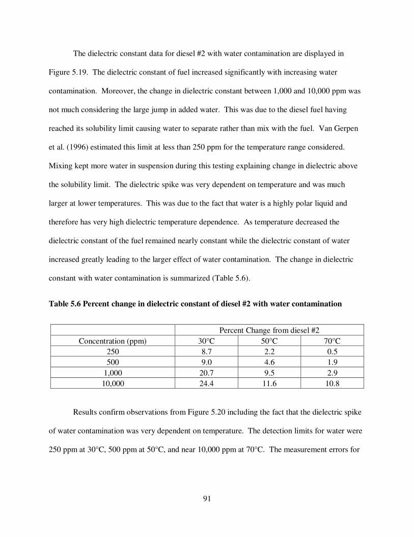
91
The dielectric constant data for diesel #2 with water contamination are displayed in
Figure 5.19. The dielectric constant of fuel increased significantly with increasing water
contamination. Moreover, the change in dielectric constant between 1,000 and 10,000 ppm was
not much considering the large jump in added water. This was due to the diesel fuel having
reached its solubility limit causing water to separate rather than mix with the fuel. Van Gerpen
et al. (1996) estimated this limit at less than 250 ppm for the temperature range considered.
Mixing kept more water in suspension during this testing explaining change in dielectric above
the solubility limit. The dielectric spike was very dependent on temperature and was much
larger at lower temperatures. This was due to the fact that water is a highly polar liquid and
therefore has very high dielectric temperature dependence. As temperature decreased the
dielectric constant of the fuel remained nearly constant while the dielectric constant of water
increased greatly leading to the larger effect of water contamination. The change in dielectric
constant with water contamination is summarized (Table 5.6).
Table 5.6 Percent change in dielectric constant of diesel #2 with water contamination
Percent Change from diesel #2
Concentration (ppm) 30°C 50°C 70°C
250 8.7 2.2 0.5
500 9.0 4.6 1.9
1,000 20.7 9.5 2.9
10,000 24.4 11.6 10.8
Results confirm observations from Figure 5.20 including the fact that the dielectric spike
of water contamination was very dependent on temperature. The detection limits for water were
250 ppm at 30°C, 500 ppm at 50°C, and near 10,000 ppm at 70°C. The measurement errors for

92
dielectric sensor were less than viscosity but greater than density. Observation led to an estimate
of these errors at 2%.
Water contamination data was also collected from blends of diesel and SME biodiesel at
levels of B-30, B-50, B-70, and B-100 (Table 5.7). Van Gerpen et al. (1996) studied water
contamination of fuels and concluded that biodiesel had much higher water solubility than diesel
#2. Therefore, it was expected that the other fuels tested would show larger changes in
properties.
Table 5.7 Percent change of viscosity of B-0, B-30, B-50, B-70, and B-100 with water
Concentration (ppm)
250 500 1,000 10,000
Temperature Percent Change
Diesel #2
30°C 0.4 3.3 23.8 15.4
50°C -0.9 1.6 9.1 10.6
70°C -4.3 -1.1 5.1 13.5
B-30
30°C -1.2 0.4 1.2 5.3
50°C -0.9 1.4 1.6 4.4
70°C -3.6 -2.2 -1.5 -0.6
B-50
30°C -0.5 10.1 6.6 27.3
50°C 3.2 7.8 6.3 16.4
70°C 0.9 5.8 5.2 7.3
B-70
30°C 0.2 1.5 2.0 3.5
50°C -4.5 -2.4 -2.8 -3.6
70°C -1.0 7.7 2.5 -0.8
B-100
30°C -0.7 4.3 -2.8 -2.8
50°C 3.3 3.7 -0.4 -1.9
70°C 3.0 10.5 1.0 4.4
Average
30°C -0.4 3.9 6.2 9.7
50°C 0.1 2.4 2.7 5.2
70°C -1.0 4.1 2.5 4.8

93
Table 5.7 contains a great deal of data that might be difficult to interpret, although
common trends were apparent. Average changes were tabulated to help provide clarity. At 250
ppm there was no effect on viscosity. At 500 and 1,000 ppm there was a measurable effect;
however, at these levels there were as many samples that show no change as that do. At 10,000
ppm there was a larger change in viscosity. In general, the spike in viscosity increased with
decreasing temperature as was observed with diesel #2. In addition the data was much more
variable and erratic at higher water contamination because of the heterogeneous mixing of water
and fuel which caused errors in measurement. The sensor required that the fluid around the
sensing element be well mixed for accuracy. This led to the varied effects observed across fuel
samples. Furthermore, the addition of more water did not always cause a large spike in viscosity
since the solubility limit of the fuel was likely surpassed.
Table 5.8 contains the results of water contamination on density measurements of the
same range of blended fuels. The results were much more consistent compared to viscosity and
all cases followed very similar trends to the results discussed for diesel #2.

94
Table 5.8 Percent change of density of B-0, B-30, B-50, B-70, and B-100 under water
contamination
Concentration (ppm)
250 500 1,000 10,000
Temperature Percent Change
Diesel #2
30°C 0.10 0.28 1.12 1.19
50°C 0.20 0.21 0.38 0.63
70°C 0.18 0.22 0.47 0.33
B-30
30°C 0.37 0.41 0.45 1.38
50°C 0.22 0.22 0.24 0.49
70°C 0.20 0.23 0.34 0.57
B-50
30°C 0.26 0.49 0.63 0.49
50°C -0.03 0.16 0.29 0.18
70°C 0.13 0.20 0.40 -0.43
B-70
30°C 0.01 0.03 0.20 0.25
50°C 0.19 0.22 0.22 0.18
70°C -0.04 -0.16 -0.01 -0.01
B-100
30°C 0.16 0.09 0.51 0.61
50°C -0.05 0.00 0.25 0.51
70°C 0.02 0.03 0.11 0.39
Average
30°C 0.18 0.26 0.58 0.79
50°C 0.11 0.16 0.28 0.40
70°C 0.10 0.10 0.26 0.17
Inspection of percent change calculations show that there was very little effect on density
by water contamination. The property was expected to increase at higher water concentrations
because water has a density approximately 25% higher than fuel. Average values showed that
density would increase more from water addition at lower temperatures. Also, the senor’s ability
to accurately measure density did not seem to be affected by heterogeneous mixing in contrast to
viscosity.

95
Table 5.9 Percent change of dielectric constant of B-0, B-30, B-50, B-70, and B-100 under
water contamination
Concentration (ppm)
250 500 1,000 10,000
Temperature Percent Change
Diesel #2
30°C 8.73 9.06 20.66 24.36
50°C 2.22 4.60 9.49 11.62
70°C 0.51 1.89 2.90 10.81
B-30
30°C 1.84 6.13 6.16 49.17
50°C 1.77 4.04 2.78 36.63
70°C 0.27 0.29 0.82 9.23
B-50
30°C 4.19 17.17 13.19 27.38
50°C 1.55 6.38 11.75 29.64
70°C 0.59 1.53 2.96 26.54
B-70
30°C 1.59 4.31 6.50 10.95
50°C 1.06 1.28 3.02 5.02
70°C 0.51 0.52 1.51 6.80
B-100
30°C 2.55 1.55 5.23 13.31
50°C 1.24 1.01 6.79 8.27
70°C 0.45 0.70 0.90 5.52
Average
30°C 3.78 7.64 10.35 25.03
50°C 1.57 3.46 6.77 18.24
70°C 0.47 0.99 1.82 11.78
Table 5.9 details the percent change of the dielectric constant output for fuels with water
contamination. The dielectric constant was the property most affected by water contamination
which was because of the high polarity and dielectric constant of water. In addition, the
dielectric constant change due to water addition was also the most temperature dependent as
evidenced by the average percent change. Water contamination would be detected by a spike in

96
the dielectric constant output. The detection limit was 250 ppm at 30°C, 500 ppm at 50°C and
somewhere between 1,000 and 10,000 ppm at 70°C. The detection limits were strongly
dependent on temperature
5.3.2 Sulfur
Baseline testing on sulfur in fuels was discussed in Section 5.1.2; this experimentation
concluded that sulfur might have an effect on the dielectric constant of fuel but that more work
was needed to quantify this effect. This section covers more testing of fuel with varying sulfur
content. Figure 5.20 shows the dielectric constant of diesel #2 with varying levels of
Dibenzothiophene, a sulfur analog in diesel fuels.
Figure 5.20 Dielectric constant of diesel #2 with sulfur contamination
2.02
2.04
2.06
2.08
2.10
2.12
2.14
2.16
0 10 20 30 40 50 60 70 80
Die
lect
ric
Co
nst
an
t
Temperature °C
Diesel #2
1000 ppm
2000 ppm
5000 ppm
10000 ppm

97
Figure 5.20 reveals that the dielectric constant of diesel fuel increased as sulfur content
increases (variation up to 1.5%); however, this increase was detectable at levels much higher
than the 15 ppm regulation. This result was less promising than the initial data taken on sulfur as
the dielectric spike was not as significant. Moreover, in the detection limit for sulfur based on
the two experiments was in the range of 1,000-5,000 ppm.
To summarize the sulfur effect and provide validation for the assertion that density and
viscosity were not significantly changed. Table 5.10 gives percent change data for diesel #2 with
sulfur contamination.
Table 5.10 Properties of diesel #2 with sulfur contamination
Concentration (ppm)
Percent Change
Temperature 1,000 2,000 5,000 10,000
Viscosity
30°C 0.33 -0.30 -0.68 1.24
50°C 4.59 2.05 1.98 5.36
70°C 4.05 1.60 2.26 5.74
Concentration (ppm)
Percent Change
Temperature 1,000 2,000 5,000 10,000
Density
30°C 0.03 0.18 0.20 0.25
50°C 0.04 0.09 0.16 0.10
70°C -0.07 0.05 0.04 0.02
Concentration (ppm)
Percent Change
Temperature 1,000 2,000 5,000 10,000
Dielectric Constant
30°C -0.09 0.03 0.84 1.32
50°C 0.13 0.08 0.24 0.56
70°C 0.17 0.47 0.31 0.74
There was very little change in density or viscosity of the fuel with added sulfur
considering the natural variation in the measurement. Additionally, there was a slight increase in

98
dielectric constant at high sulfur concentrations, and this dielectric spike was independent of
temperature.
5.3.3 Urea
Another contaminant tested was urea in the form of DEF, diesel exhaust fluid. This urea
based liquid is used in some exhaust after-treatment systems and must be refilled occasionally.
Refilling of fuel and DEF would often occur at the same time allowing for the possibility of
cross contamination due to operator error. This set of tests evaluated the sensor for protection
against accidental addition of DEF to the fuel tank (Figures 5.21, 5.22, and 5.23).
Figure 5.21 Dynamic viscosity of diesel #2 with urea contamination
0.00
0.50
1.00
1.50
2.00
2.50
3.00
3.50
0 10 20 30 40 50 60 70 80
Dy
na
mic
Vis
cosi
ty (
cP)
Temperature °C
B-50
1000 ppm
2000 ppm
5000 ppm
10,000 ppm

99
Figure 5.22 Density of diesel #2 with urea contamination
Figure 5.23 Dielectric constant of diesel #2 with urea contamination
0.78
0.79
0.80
0.81
0.82
0.83
0.84
0 10 20 30 40 50 60 70 80
De
nsi
ty (
g/m
l)
Temperature °C
B-50
1000 ppm
2000 ppm
5000 ppm
10,000 ppm
1.00
1.20
1.40
1.60
1.80
2.00
2.20
2.40
2.60
2.80
0 10 20 30 40 50 60 70 80
Die
lect
ric
Co
nst
an
t
Temperature °C
B-50
1000 ppm
2000 ppm
5000 ppm
10000 ppm

100
Figures 5.21, 5.22, and 5.23 suggest that the addition of urea to fuel had an effect on all
three of the sensor outputs, although the change in dielectric was much larger than that of
viscosity and density.
Blends of SME biodiesel and diesel #2 at levels of B-30 and B-50 were also tested for
urea contamination. Tables 5.11, 5.12, and 5.13 summarize the percent change due to
contamination for each of viscosity, density, and dielectric constant respectively over this range
of fuels.
Table 5.11 Percent change of dynamic viscosity with urea contamination
Concentration (ppm)
1,000 2,000 5,000 10,000
Temperature Percent Change
Diesel #2
30°C 1.73 9.98 12.36 12.01
50°C 5.68 20.89 14.70 16.35
70°C 1.09 18.28 13.92 14.30
B-30
30°C 1.81 0.98 3.69 5.00
50°C 7.38 8.01 6.63 9.07
70°C 2.25 14.62 8.59 16.52
B-50
30°C 0.89 7.02 5.07 -4.52
50°C 5.67 6.78 7.22 -3.25
70°C 6.69 8.74 8.13 -0.15

101
Table 5.12 Percent change of density with urea contamination
Concentration (ppm)
1,000 2,000 5,000 10,000
Temperature Percent Change
Diesel #2
30°C 0.09 0.21 0.46 1.01
50°C 0.14 0.45 0.45 0.87
70°C 0.08 0.15 0.33 0.55
B-30
30°C 0.23 0.08 0.59 0.77
50°C 0.24 0.20 0.49 0.95
70°C 0.03 -0.21 0.37 0.23
B-50
30°C 0.48 2.31 3.04 0.69
50°C 1.39 3.00 3.08 0.39
70°C 0.89 2.75 2.70 0.27
Table 5.13 Percent change of dielectric constant with urea contamination
Concentration (ppm)
1,000 2,000 5,000 10,000
Temperature Percent Change
Diesel #2
30°C 1.29 2.70 19.18 15.74
50°C 0.49 3.22 10.57 18.82
70° C 0.45 3.83 8.69 17.67
B-30
30°C 5.58 8.53 19.11 22.63
50°C 4.68 3.66 21.79 32.80
70°C 2.13 2.38 25.70 48.60
B-50
30°C 1.13 6.28 11.95 16.07
50°C 0.52 7.64 10.51 11.35
70°C 0.42 5.24 9.12 13.89

102
Analysis of the urea contamination results showed few consistent trends. Although the
addition of urea tended to increase the dielectric constant significantly and the viscosity and
density to a lesser level it was difficult to use this data for algorithm development. The high
variability of the effect of urea was a product of the urea tending to crystallize into small solids
in the fuel. These solids would stick to the sensing element and caused very inaccurate
measurements. Urea contamination could be detected by the sensor but at high concentrations it
would introduce considerable error into the prediction capability of the sensor.
5.3.4 Glycerol
SME biodiesel and blends with diesel #2 were tested with varying glycerol amounts
added. Figure 5.24 gives dynamic viscosity results for SME B-100.
Figure 5.24 Dynamic viscosity of SME B-100 with glycerol contamination
0.00
1.00
2.00
3.00
4.00
5.00
6.00
7.00
8.00
9.00
0 10 20 30 40 50 60 70 80
Dy
na
mic
Vis
cosi
ty (
cP)
Temperature °C
B-100
250 ppm
500 ppm
1000 ppm
10,000 ppm

103
Viscosity was affected considerably by the addition of free glycerin to the fuel sample at
concentrations above 1,000 ppm. However, the effect was small at levels below 1,000 ppm. The
viscosity of pure glycerol is approximately one hundred times greater than that of fuel so this
increase in viscosity was not surprising. The phenomenon was very temperature dependent with
the viscosity increase largest at low temperatures. These results agreed with Van Gerpen et al.
(1996) whose experiments also showed significant increases in viscosity with glycerin addition.
Figure 5.25 Density of SME B-100 with glycerol contamination
The density of SME B-100 under the same glycerol addition is plotted in Figure 5.25.
Glycerol contamination had a larger effect on density measurements than any of the other
contaminants tested in this study. Moreover, pure glycerol has a density of 1.261 g/ml which is
also the highest of any of the contaminants. The change in density was largest at lower
0.83
0.84
0.85
0.86
0.87
0.88
0.89
0.90
0.91
0.92
0 10 20 30 40 50 60 70 80
De
nsi
ty (
g/m
l)
Temperature °C
B-100
250 ppm
500 ppm
1000 ppm
10,000 ppm

104
temperatures. This suggested that the temperature dependence of density for glycerol was
greater than for fuel samples. In cases of high glycerol contamination the density measurement
was affected sufficiently to make fuel type determination by use of this sensor output very
inaccurate.
The dielectric constant was also increased in the case of glycerol addition. Figure 5.26
details the results.
Figure 5.26 Dielectric constant of SME B-100 with glycerol contamination
The dielectric constant was moderately changed with glycerol addition. Concentrations
below 1,000 ppm seemed to have little effect. In general, the amount of dielectric spike
increased with decreasing temperature.
2.00
2.50
3.00
3.50
4.00
4.50
0 10 20 30 40 50 60 70 80
Die
lect
ric
Co
nst
an
t
Temperature C
B-100
250 ppm
500 ppm
1000 ppm
10000 ppm

105
Several blends were also tested for glycerol pollution. Tables 5.14, 5.15, and 5.16
summarize the percent change of each of viscosity, density, and dielectric constant respectively
for blends of SME B-100 with diesel #2 under several glycerol contamination concentration
levels.
Table 5.14 Percent change in dynamic viscosity for fuels with glycerol contamination
Concentration (ppm)
250 500 1,000 10,000
Temperature Percent Change
B-100
30°C 1.5 16.9 22.3 86.0
50°C 1.9 16.6 14.5 81.9
70°C 2.3 17.9 7.3 27.8
B-70
30°C 9.2 10.3 20.4 24.3
50°C 8.3 9.6 18.3 25.1
70°C 8.7 11.3 22.5 16.7
B-50
30°C 9.4 5.2 30.7 101.1
50°C 5.4 2.4 23.2 92.8
70°C 0.5 1.6 10.9 45.1
B-30
30°C 17.4 16.4 30.6 30.5
50°C 13.0 13.8 31.2 -2.2
70°C 2.7 3.6 8.4 0.2
Average
30°C 9.4 12.2 26.0 60.5
50°C 7.2 10.6 21.8 49.4
70°C 3.6 8.6 12.3 22.4

106
Table 5.15 Percent change in density for fuels with glycerol contamination
Concentration (ppm)
250 500 1,000 10,000
Temperature Percent Change
B-100
30°C 0.21 -0.27 2.53 4.44
50°C -0.06 -0.66 0.33 3.03
70°C 0.05 -0.49 0.14 0.75
B-70
30°C 0.95 1.12 2.65 2.32
50°C 0.76 0.83 1.06 1.33
70°C 0.89 0.95 0.67 1.10
B-50
30°C -0.05 0.37 2.36 4.71
50°C -0.08 0.16 1.12 3.83
70°C -0.11 0.04 0.39 1.81
B-30
30°C 1.95 2.13 2.76 2.41
50°C 1.25 1.60 2.89 0.43
70°C 1.07 1.05 1.02 0.14
Average
30°C 0.76 0.84 2.57 3.47
50°C 0.47 0.48 1.35 2.16
70°C 0.47 0.39 0.55 0.95

107
Table 5.16 Percent change in dielectric constant for fuels with glycerol contamination
Concentration (ppm)
250 500 1,000 10,000
Temperature Percent Change
B-100
30°C 1.1 2.7 12.8 33.2
50°C 1.1 0.8 7.3 36.7
70°C 0.4 0.5 2.6 15.6
B-70
30°C 6.6 7.3 15.8 15.8
50°C 6.5 6.6 10.3 12.6
70°C 6.4 6.4 7.2 9.0
B-50
30°C 0.3 2.3 17.2 41.6
50°C 0.4 0.9 17.7 40.5
70°C -0.1 0.4 6.2 37.9
B-30
30°C 1.4 5.9 7.1 9.0
50°C 3.1 7.1 10.1 9.6
70°C 1.5 1.7 4.5 9.4
Average
30°C 2.3 4.6 13.2 24.9
50°C 2.8 3.9 11.4 24.9
70°C 2.0 2.2 5.1 18.0
Percent change calculations show that viscosity was the property impacted the most by
glycerol addition followed by dielectric constant and then density. All three sensor outputs
showed more change at lower temperatures. Glycerol contamination would not be as easily
interpreted by basic algorithms because all three outputs were significantly affected leaving no
outputs to determine fuel type prior to detecting contamination. However, glycerol
contamination above the ASTM standard of 1,900 ppm should be measurable. No trends were
evident with changing blend level. The most important variable defining the deviations in
change between fuel samples was likely heterogeneous mixing.

108
5.3.5 Methanol
Methanol was another potential contaminant of biodiesel, and consequently was used to
dope fuel samples for testing with the MEAS sensor. Sensor outputs under various levels of
contamination for SME B-100 were measured, and dielectric constant was found to be the only
output appreciably altered (on average, viscosity variation under 3.0% and density variation
under 0.25%). Figure 5.27 contains dielectric measurements for SME B-100 under methanol
contamination.
Figure 5.27 Dielectric constant of SME B-100 with methanol contamination
Dielectric constant increased with methanol addition as would be expected because the
dielectric constant of pure methanol is 32.5. Methanol addition below 5,000 ppm was not
2.85
2.90
2.95
3.00
3.05
3.10
3.15
3.20
3.25
0 10 20 30 40 50 60 70 80
Die
lect
ric
Co
nst
an
t
Temperature C
B-100
1000 ppm
2000 ppm
5000 ppm
10000 ppm

109
detectable. Tat and Van Gerpen (2003b) reported the dielectric spike with methanol addition to
be much less than what is suggested by Figure 5.27. The discrepancy was tied to the difference
between sensors used for measurement.
Tables 5.17, 5.18, and 5.19 contain viscosity, density, and dielectric changes for several
fuels with methanol contamination.
Table 5.17 Percent change in dynamic viscosity of fuels with methanol contamination
Concentration (ppm)
1,000 2,000 5,000 10,000
Percent Change
B-100
30°C 1.9 -7.5 -6.2 -7.1
50°C -2.4 -4.3 -3.7 -8.7
70°C -0.2 -0.5 4.6 -3.4
B-70
30°C -6.9 -3.5 -7.1 -6.2
50°C -3.8 -1.9 -3.9 -3.9
70°C 0.9 0.6 2.1 0.1
B-30
30°C -2.6 2.1 4.5 11.0
50°C -4.8 -0.7 -0.8 5.5
70°C -2.6 4.9 1.7 6.9
Average
30°C -2.5 -3.0 -2.9 -0.8
50°C -3.6 -2.3 -2.8 -2.4
70°C -0.6 1.6 2.8 1.2

110
Table 5.18 Percent change in density of fuels with methanol contamination
Concentration (ppm)
1,000 2,000 5,000 10,000
Percent Change
B-100
30°C 0.01 0.15 0.21 0.33
50°C 0.18 0.16 0.08 0.26
70°C 0.10 0.00 0.00 0.13
B-70
30°C 0.26 -0.06 0.32 0.09
50°C 0.33 0.23 0.37 0.27
70°C 0.02 0.06 0.06 0.06
B-30
30°C 0.09 -0.13 0.04 -0.23
50°C 0.20 0.19 0.26 -0.01
70°C 0.20 0.05 0.21 0.23
Average
30°C 0.12 -0.01 0.19 0.06
50°C 0.24 0.19 0.24 0.17
70°C 0.11 0.04 0.09 0.14
Table 5.19 Percent change in dielectric constant of fuels with methanol contamination
Concentration (ppm)
1,000 2,000 5,000 10,000
Percent Change
B-100
30°C -0.5 -0.2 1.1 1.9
50°C -0.1 0.2 0.9 1.7
70°C 0.0 0.4 0.9 1.5
B-70
30°C 0.4 0.7 1.5 3.1
50°C 0.3 0.5 1.2 2.5
70°C 0.2 0.4 0.9 1.7
B-30
30°C -0.7 -0.4 0.9 11.3
50°C -0.2 0.2 0.9 5.9
70°C 0.0 0.3 0.6 1.4
Average
30°C -0.2 0.0 1.1 5.4
50°C 0.0 0.3 1.0 3.4
70°C 0.1 0.4 0.8 1.5

111
Tables 5.17 through 5.19 confirm that the density and viscosity of fuels were not largely
changed by methanol addition. Also, the dielectric constant was affected measurably at
methanol concentrations greater than 5,000 ppm. Furthermore, methanol contamination had the
largest effect at low temperatures.
5.3.6 Summary of Results
Five contaminants of fuel were experimented with in order to determine the effect these
contaminants have on the properties of fuels, and to gauge whether the MEAS sensor would be
able to discern contaminated fuels from clean fuels. Results showed that for all of the
contaminants tested if concentrations in the fuel were high enough there would be a measurable
effect on fuel properties (Table 5.20).
Table 5.20 Summary of contamination effects
Fuel Situation Viscosity Density Dielectric Constant
Water contamination small increase small increase large increase
Urea contamination small change/ erratic small change/erratic large change/erratic
Glycerol contamination large increase small increase large increase
Methanol contamination no change no change medium increase
Sulfur contamination no change no change small increase
For each contaminant an approximate detection limit with the MEAS sensor could be set.
Taking into account the natural variation in fuel properties table it is possible to provide
estimates the detection limits for each contaminant (Table 5.21).

112
Table 5.21 Detection limits for various contaminants
Contaminant Water Sulfur Urea Glycerol Methanol
Temperature °C 30-70 30-70 30-70 30-70 30-70
Detection Limit (ppm) 250-1,000 5,000-10,000 2000 1,000-10,000 5,000
ASTM Standard 500 ppm 15 ppm NA 1,900 ppm 2,000 ppm
Detection limits meet ASTM standards at most temperatures for water and glycerol.
Methanol and urea were also detectable but must be present in higher concentrations.
Furthermore, detection limits were very temperature dependent. Lower temperatures led to more
effective contaminant detection in all cases (below 50°C). This suggested that the sensor should
be placed closer to the fuel tank in order to measure fuel near ambient conditions. When fuel
was contaminated sensor outputs were more variable and less accurate because of the effect of
heterogeneous mixing. If the fluid surrounding the sensing element contained a droplet of
contaminant the sensor’s outputs were greatly changed. It was expected that fuel type and blend
prediction algorithms would be less accurate in the case of contaminated fuels. Moreover, while
contaminants were easily discerned from observation of sensor outputs when fuel type was
known, it was a much more complicated problem to detect contamination when fuel type was
also unknown which was the case faced by fuel composition sensors in real applications. Section
5.6 discusses the development of algorithms that provide solutions to this issue.
5.4 Effect of Fuel Degradation on Sensor Outputs
As fuel degrades its properties change, allowing this condition to be detectable to the
MEAS sensor. Although the exact consequences of combusting degraded fuel are not well
defined, it is less than ideal to use degraded fuel. Engine manufacturers feel that identifying

113
degraded fuel could add value to engines despite conflicting literature on how detrimental
combusting degraded fuel actually is. The effects of degradation on sensor response for several
fuel samples are summarized in the following figures. Results for open container samples of
diesel #1, diesel #2, and SME B-100 were plotted (Figure 5.28).
Figure 5.28 Effect of time on the dynamic viscosity of several fuels
It can be seen that the viscosity of all three fuels increased with time. The result was very
dramatic for diesel #1 and diesel #2 with viscosity increasing by more than 50% of the original
value. The literature review suggested that biodiesel would be more susceptible to degradation
than petroleum based fuels. However, these results indicated the degradation of the petroleum
based fuels was much more observable by the MEAS sensor than for biodiesel. The change in
viscosity for biodiesel was in a similar range to findings from Bondioli et al. (2003). The
1.00
1.50
2.00
2.50
3.00
3.50
4.00
4.50
5.00
0 50 100 150 200 250 300 350 400 450
Dy
na
mic
Vis
cosi
ty (
cP)
Time (days)
Diesel #1
Diesel #2
SME B-100

114
variation observed in the trends was partially due to changes in the temperature at time of
measurement between each case.
Figure 5.29 Effect of time on the density of several fuels
Figure 5.29 summarizes the density of open container fuels samples with time. The
density of the fuels was nearly constant over the entire measurement time period. Moreover, a
comparison of the density measurement to the viscosity measurement would be an effective way
to detect degraded fuel.
0.70
0.75
0.80
0.85
0.90
0.95
1.00
0 50 100 150 200 250 300 350 400 450
De
nsi
ty (
g/m
l)
Time (days)
Diesel #1
Diesel #2
SME B-100

115
Figure 5.30 Effect of time on the dielectric constant of several fuels
Figure 5.30 presents the dielectric constant output against time. As with the density
output, the dielectric constant measurement from the MEAS sensor did not appear to change as
fuel samples age.
Figures 5.31 through 5.33 present results for measurements from closed container fuel
samples over a 580 day time period. Data was not available for a several month period near the
beginning of the study.
0.00
0.50
1.00
1.50
2.00
2.50
3.00
3.50
4.00
0 50 100 150 200 250 300 350 400 450
Die
lect
ric
Co
nst
an
t
Time (days)
Diesel #1
Diesel #2
SME B-100

116
Figure 5.31 Effect of time on the dynamic viscosity of several fuels
The viscosity once again increased with age for the closed container samples although the
effect was not as pronounced as indicated in Figure 5.31. The change was approximately the
same for each of the three fuels and was in the range of 6-12%. A peak in viscosity
measurements was observed late in the time period for unknown reasons
1.00
1.50
2.00
2.50
3.00
3.50
4.00
0 100 200 300 400 500 600 700
Dy
na
mic
Vis
cosi
ty (
cP)
Time (days)
Diesel #1
Diesel #2
SME B-100

117
Figure 5.32 Effect of time on the density of several fuels
Figure 5.33 Effect of time on the dielectric constant of several fuels
0.70
0.75
0.80
0.85
0.90
0.95
1.00
0 100 200 300 400 500 600 700
De
nsi
ty (
g/m
l)
Time (days)
Diesel #1
Diesel #2
SME B-100
0.00
0.50
1.00
1.50
2.00
2.50
3.00
3.50
0 100 200 300 400 500 600 700
Die
lect
ric
Co
nst
an
t
Time (days)
Diesel #1
Diesel #2
SME B-100

118
Figures 5.32 and 5.33 display sensor results for the density and dielectric constant
outputs. It can be seen that the density and dielectric constant were nearly constant with ageing
for these fuels samples. Based on the above results degraded fuel would show an increased
viscosity over fresh fuels while having unchanged density and dielectric properties. Moreover,
an algorithm employing a comparison of either the density or dielectric constant measurement
with the viscosity measurement would be successful at identifying degraded fuels.
5.5 Development of a Fuel Classification Model
General results for the form and accuracy of models applied to the data are conveyed in
this chapter. In addition the use of these models in the design of an algorithm for fuel type and
quality detection is described.
5.5.1 Algorithm Format
The base algorithm proposed for use in the MEAS sensor involved a series of decisions
based on sensor outputs. This series of logic sought to determine the type of diesel fuel that was
being used, the level to which this fuel was blended with biodiesel, the contamination level of the
fuel, and the degradation level of the fuel.
The first step in fuel type determination was to decide if diesel #1 or diesel #2 is the
primary fuel. As was seen in Section 5.2.3 density is the ideal output to use for this since it was
minimally affected by contaminants and it did not overlap for diesel #1 blends up to B-20 and
diesel #2 blends. Therefore, the algorithm used a linear split on the density scale dependent on
temperature to determine within which blending regime the fuel fell (Figure 5.34).

119
Figure 5.34 Base fuel determinations relative to density output
Once the base fuel had been set the blend percentage was calculated. The algorithm first
calculated the properties of the neat fuels at the measured temperature. For example, if the base
fuel was diesel #2, six properties (the dynamic viscosity, density, and dielectric constant of pure
diesel #2 and SME B-100) were calculated using temperature regression models. Next, the
algorithm took the measured density and dielectric outputs and linearly interpolated between the
two calculated values for neat fuels and returned two estimates for blend percentage. The
viscosity output was also interpolated but it was not linear as described in Table 4.8. Finally,
there were three estimates for blend percentage. The three results were averaged to give the final
blend approximation. Testing of this part of the algorithm for uncontaminated fuels gave blend
prediction accuracy at three percent or better.

120
For contaminated fuels blend prediction gave errors up to 30% if no other compensation
was included. Water contamination and degradation were the most important of the fuel
conditions studied so the algorithm development focused on these effects. The algorithm
provided the predicted dielectric constant of the fuel based on the measured viscosity. This value
was compared to the measured dielectric constant. As is shown in more detail in Section 5.5.5 a
relationship had been developed for the difference between these two values over varying
temperature and contamination levels. If the difference was close to zero the algorithm indicated
that the fuel was clean and the original blend estimate was specified. If the difference was
positive this indicated that there was water contamination at some level. If it was negative the
fuel was considered degraded. The average change of each output over the clean fuel output for
varied temperature and contamination had also been compiled so the estimated contamination
level could give an adjusted property that was close to that of the clean fuel. Finally, this
adjusted value was entered into the blend prediction interpolations. This method would decrease
blend prediction error to 10% or less.
5.5.2 Regression Models for Fuel Properties with Temperature
Inspection of the plots created for sensor outputs discussed in Section 5.1.1 gave some
information about the type of models that may describe the dependence of each output on
temperature. Furthermore, the MEAS sensor’s temperature measurement was an essential output
for accurate prediction of fuel composition. Temperature was used to estimate uncontaminated
properties of possible fuels which could then be used to compare with the measured outputs.
Section 4.7.2 summarizes the models used to fit the data. Figure 5.35 shows dynamic viscosity
data with curve fitting for several fuels.

121
Figure 5.35 Dynamic viscosity curve fits
Data fits for viscosity with temperature were developed using the model described in
Table 4.8. The model fit very well giving minimum R2 = .9996.

122
Figure 5.36 Density curve fits
The density outputs were also modeled as shown in Figure 5.36. Density was predicted
with a linear relationship with temperature. Each of the fuels had a linear fit with approximately
the same slope (less than 0.5% variation). Accuracy of the fits was a minimum R2 = .9972.
0.74
0.76
0.78
0.80
0.82
0.84
0.86
0.88
0.90
0 10 20 30 40 50 60 70 80 90
De
nsi
ty (
g/m
l)
Temperature °C
Diesel #1
Diesel #2
Jet A
SME B-100
Linear (Diesel #1)
Linear (Diesel #2)
Linear (Jet A)
Linear (SME B-100)

123
Figure 5.37 Dielectric constant curve fits
Figure 5.37 contains the data for dielectric constants of the same fuels and temperature
range. The dielectric constant was also very accurately modeled by a simple linear model. The
slope of this model did vary for the type of fuel. The accuracy was apparent from R2 >.9971.
5.5.3 Regression Models for Fuel Properties with Blend
In order to interpolate between the calculated values of the two pure fuels in a blend a
model must be established for the way each property changes with blend percentage. Models
used for this purpose are described in Table 4.8 (Tat and Van Gerpen, 1999; Tat and Van
Gerpen, 2000). This section gives figures showing the accuracy of fits for blends of diesel #2
and SME B-100. Figure 5.38 details both the actual data and values predicted by the model for
dynamic viscosity of blends at two different temperatures.
1.50
1.70
1.90
2.10
2.30
2.50
2.70
2.90
3.10
3.30
3.50
0 20 40 60 80 100
Die
lect
ric
Co
nst
an
t
Temperature °C
Diesel #1
Diesel #2
Jet A
SME B-100
Linear (Diesel #1)
Linear (Diesel #2)
Linear (Jet A)
Linear (SME B-100)

124
Figure 5.38 Measured and predicted dynamic viscosity for blends of fuel
The Grunberg-Nissan model was very accurate with errors of less than two percent. The
exponential shape of the viscosity blending trend was well described by the model.
0.00
0.50
1.00
1.50
2.00
2.50
3.00
3.50
4.00
4.50
0 20 40 60 80 100 120
Dy
na
mic
Vis
cosi
ty (
cP)
Blend Percentage
30 C
Predicted at 30 C
80 C
Predicted at 80 C

125
Figure 5.39 Density of diesel #2 and SME B-100 data fitting
Figure 5.39 illustrates the model fit for density. Linear models provided a close fit to the
blended fuels at each of the plotted temperatures. In addition the slope of each fit was
approximately the same (variation less than 0.5%). The accuracy of the linear model for density
of blended fuels was very high with R2 values of at least .9991.
0.79
0.80
0.81
0.82
0.83
0.84
0.85
0.86
0.87
0.88
0 20 40 60 80 100
De
nsi
ty (
g/m
l)
Blend Percentage
30 C
40 C
50 C
60 C
70 C
80 C

126
Figure 5.40 Dielectric constant of diesel #2 and SME B-100 data fitting
Figure 5.40 displays the models and data for dielectric constant with changing blend
percentage for several temperatures. For dielectric constant a simple linear model was once
again sufficient for very accurate prediction of fuel properties given the properties of the two
components in the blend. The slope of each line was not the same, however, due to the
difference in rates of change of diesel #2 and SME B-100 with temperature. R2 values were at a
minimum .9984.
5.5.4 Sensitivity and Limits of Regression Models
Another important factor in the success of the algorithm was defining the limits of its
validity and its sensitivity. This section details the limits of the algorithm with respect to
2.00
2.20
2.40
2.60
2.80
3.00
3.20
3.40
0 20 40 60 80 100
Die
lect
ric
Co
nst
an
t
Blend Percentage
30 C
40 C
50 C
60 C
70 C
80 C

127
temperature. In addition the appropriate sensitivity for the algorithm as defined by the natural
variation in fuel properties is discussed.
Testing was carried out through the upper temperature range that fuels would likely
encounter in a fuel system. Moreover, the models developed should be accurate up to this upper
temperature limit. However, the lower temperature limit that fuels would reach in cold climates
was not tested. The cloud point was the limit to which the sensor will accurately read fuel
properties so this also was set as the lower limit of the algorithm (Figure 5.41). The cloud point
for blended fuels was estimated by linearly interpolating between measured cloud points for
diesel #2 and SME B-100 found in the literature (Tables 3.4 and 3.5).
Figure 5.41 Cloud point of blends of diesel #2 and SME B-100
-18
-16
-14
-12
-10
-8
-6
-4
-2
0
0 20 40 60 80 100
Te
mp
era
ture
°C
Blend Percentage
Cloud Point

128
The lower limit of the algorithm was detected when the sensor gave erratic results at
temperatures lower than shown in Figure 5.41. At temperatures above 0°C the algorithm should
always be accurate. At temperatures below -17°C sensor results must be ignored since the
results would not fall within the valid range of the algorithm.
The algorithm also relied on the measured properties from the sensor being relatively
similar to the properties measured for fuels in this study. Moreover, the detection of
contamination or degradation should not be so sensitive as to falsely detect fuels due to normal
variation of properties from those measured in this work. Some analysis was conducted on the
natural variation of biodiesel viscosity and density. Table 5.22 summarizes results for
predictions of biodiesel viscosities for the natural ranges of fatty acid compositions.
Table 5.22 BDProp predicted natural range of viscosities for SME and RME (rapeseed
methyl ester) biodiesel
Dynamic Viscosity cP
Biodiesel Temperature °C Upper Limit Lower Limit Percent Range
SME
17 6.68 6.13 9.0
37 4.05 3.77 7.4
57 2.72 2.56 6.2
77 1.97 1.88 5.1
RME
17 9.41 8.48 11.0
37 5.61 5.12 9.6
57 3.63 3.36 8.0
77 2.50 2.35 6.4
Table 5.22 predicted similar viscosities as to what was measured for SME biodiesel;
however, it predicted higher viscosities for rapeseed biodiesel. The important conclusion was

129
that the natural variation for viscosity in biodiesel was temperature dependent and ranged from
about 5% to 10%.
Table 5.23 details the results of similar computations for the density of SME and RME
biodiesel. The natural variation in density was much less than that of viscosity. Also, the
predicted densities were very similar to what was measured for each type of biodiesel.
Table 5.23 BDProp predicted natural range of densities of SME and RME biodiesel at 20°C
Upper Limit Lower Limit Percent range
SME 0.888 0.883 0.481
RME 0.884 0.881 0.370
Based on the assumption that petroleum based fuels have less variation in properties due
to more consistent refining technologies and source compositions it could be assumed that the
ranges established for biodiesel were the worst case scenarios for variation in blended fuels.
Therefore, the sensitivity of the sensor would be in part based off of the ranges calculated above.
In addition, there existed no way of predicting dielectric constant based on fatty acid content so
an estimate would be made according to the variation observed during experimentation.
5.5.5 Identification of Contaminants or Degradation
Comparison of how fuel properties changed with added contaminants was a criterion that
would be used for contamination identification. Moreover, as discussed in Section 5.5.1
comparison of the dielectric constant predicted from the viscosity measurement to the measured
dielectric constant was the basis for both water contamination and degradation condition. This
choice is apparent from the blend prediction error calculated from equations 4.1 through 4.3
(Table 5.24).

130
Table 5.24 Calculated blend prediction error E
EViscosity EDensity EDielectric Constant
250
ppm
500
ppm
1000
ppm
10000
ppm
250
ppm
500
ppm
1000
ppm
10000
ppm
250
ppm
500
ppm
1000
ppm
10000
ppm
T
°C
30 0.02 7.00 10.07 11.91 4.14 6.01 13.24 17.76 9.13 18.97 25.21 62.24
50 1.36 5.63 6.22 7.42 2.46 3.70 6.40 9.27 4.16 8.99 18.24 48.23
70 0.55 10.78 7.29 9.99 2.16 2.27 5.75 3.84 1.35 2.74 5.09 33.37
Inspection of the table showed that calculation of the blend level became more inaccurate
with increased water addition and decreased temperature for all three outputs. Use of the
dielectric constant for blend prediction with contamination introduced the most error. Moreover,
the viscosity output was the best predictor of blend level in most cases. Therefore, the
comparison of the viscosity and dielectric constant was the best basis for contamination
detection.
Degradation was also considered in the algorithm, and a similar calculation was
undertaken to find the blend prediction error for degraded fuel as a function of fuel age. The
increase in viscosity associated with degradation caused the Eviscosity to be much higher than the
other two calculated values for density and dielectric constant.
A plot of the difference between the predicted dielectric constant from the viscosity
output and the actual dielectric constant could be used to identify both the water contamination
and degradation conditions. Figure 5.42 gives this difference for water contamination at four
concentrations over three temperatures in addition to degradation at four ages (Eqn. 4.4).

131
Figure 5.42 Calculated Ddc,η for water contaminated and degraded fuel
Figure 5.42 shows that water contamination caused the calculated difference to be
positive and increase with decreasing temperature. Values that were near zero indicated clean,
fresh fuel. In contrast as the value became more positive this indicated higher water
contamination. Large negative values were indicative of degraded fuel. At 30°C, 250 ppm water
contamination was detectable. At 50°C the detection limit rose to 1,000 ppm while at 70°C the
detection limit was near 10,000 ppm. The effect of degradation was very apparent from this plot.
-1
-0.8
-0.6
-0.4
-0.2
0
0.2
0.4
0 10 20 30 40 50 60 70
D d
c, η
Temperature °C
250 ppm
500 ppm
1000 ppm
10,000 ppm
100 Days
Degraded
200 Days
Degraded
300 Days
Degraded
370 Days
Degraded

132
Using Figure 5.42 the water contamination or degradation condition for any fuel sample
could be estimated. Once the level of contamination was known the percent change data
presented in Section 5.3.1 could be used to approximate the actual values of the fuel if it had not
been contaminated. Finally, these approximate clean fuel values could be placed into the
interpolation equations to give the blend percentage.
5.5.6 Neural Network to Identify Fuel Composition and Contamination
An alternative method for algorithm development for both blend percentage and
contamination identification was the use of a neural network. Neural networks have proven to
accurately develop models for many engine and sensor applications, and they provided a second
option for fuel composition sensing. Data from one sensor over a range of blends between diesel
#2 and SME B-100 and several water contamination levels was used to create and train a neural
net algorithm in MATLAB. MATLAB software divided the data into three sets placing 70% of
the data vectors into training, 15% into validation, and 15% into testing. The software then
automatically optimized training of the network and tested the predictive ability on the testing
data. Figure 5.43 shows the algorithms predicted blend percentage values vs. the actual values.
Contamination levels 0.0, 0.25, 0.5, 1.0, and 2.0 referred to water concentrations of 250 ppm,
500 ppm, 1,000 ppm, and 10,000 ppm respectively.

133
Figure 5.43 Neural network prediction of blend percentage
The neural network generated accurate predictions for blend percentage in the case of
using one sensor to develop the algorithm and the same sensor’s outputs to test it. The mean
square error was less than 3.1 for training, validation, and test data for this case, and the R2 value
was above .99. Moreover, errors of less than 4% were predicted by the network.
In addition the actual values and predicted values for contamination condition were
plotted. Figure 5.44 presents these results.
R² = 0.9998
0
10
20
30
40
50
60
70
80
90
100
0 20 40 60 80 100
Ble
nd
% P
red
icte
d
Actual Blend %
Neural Net Blend
Linear (Neural Net Blend)

134
Figure 5.44 Neural network prediction of contamination conditions
The network was less accurate at predicting contamination level, particularly at higher
blend percentages. The mean square error for this case was below 8.0 and the R2 = .892.
Addition of water added variability to the data resulting in less accurate results. Also, higher
contamination levels led to greater variability. This was still a positive result however since
contamination levels of 1 and 2 were entirely distinguishable from clean fuel samples. It was
desirable that at the minimum the algorithm could identify the higher contamination levels and
not give false positive readings for clean fuel.
Figures 5.43 and 5.44 represent ideal conditions in which the same sensor was used for
both algorithm development and testing. Observation of contamination results for several
R² = 0.892
-0.5
0
0.5
1
1.5
2
2.5
3
0 0.5 1 1.5 2 2.5
Pre
dic
ted
Co
nta
min
ati
on
Co
nd
itio
n
Actual Contamination Condition
Neural Net Cont.
Linear (Neural Net Cont.)

135
different sensors indicated that each sensor showed different magnitude of changes from a given
contamination concentration. Therefore, a more accurate assessment of neural network
software’s ability to predict fuel conditions was to develop the model based on data from several
sensors. Figure 5.45 shows actual blend percentage vs. predicted blend percentage for a neural
network model using three sensors for both development and testing.
Figure 5.45 Neural network predictions for blend percentage with multiple sensor data
Again, the network accurately predicted blend percentage in the case of multiple sensor
data. The mean square error and R2 values were similar to figure 5.43. Moreover, errors of less
than 5% would be expected from this model.
R² = 0.9995
0
10
20
30
40
50
60
70
80
90
100
0 20 40 60 80 100
Pre
dic
ted
Ble
nd
%
Actual Blend %
Neural Net BlendLinear (Neural Net …

136
Figure 5.46 Neural network predictions for contamination condition with multiple sensor
data
Figure 5.46 shows the contamination prediction results for multiple sensor data. As
expected the performance of the neural network approach with respect to predicting
contamination condition decreased considerably when including the effect of multiple sensors.
The R2 value for this plot was much lower at .565. More importantly, there was overlap between
the predicted conditions of clean fuel and the highest contamination level. This result indicated
that the model would not be sufficiently accurate, and would potentially identify clean fuel as
being contaminated.
R² = 0.5651
-1
-0.5
0
0.5
1
1.5
2
2.5
3
0 0.5 1 1.5 2 2.5
Pre
dic
ted
Co
nta
min
ati
on
Co
nd
itio
n
Actual Contamination Condition
Neural Net Cont.
Linear (Neural Net Cont.)

137
5.5.7 Summary of Results
An algorithm for the detection of water contaminated and degraded fuel in addition to
blend percentage determination was developed based on models fitted to fuel data taken over a
wide range of temperatures and blends. Linear models were applied to the behavior of the
density and dielectric constant outputs with both temperature and blend percentage. Non-linear
models were needed to describe the behavior of the dynamic viscosity for both temperature and
blend percentage. Furthermore, the density output was employed to distinguish between blends
of diesel #1 and blends of diesel #2. All three outputs were used to estimate the blend
percentage for clean fuels. In addition contamination by water and degradation was detected by
comparison of the viscosity and dielectric outputs from the MEAS sensor. In the condition that
the measured dielectric constant was higher than the dielectric constant predicted by the viscosity
water contamination was present. For degraded fuel the predicted dielectric constant would be
higher than the actual value.
Neural networks were also used to develop and algorithm based on fuel data. Data from
a single sensor were consistent enough to create an accurate model for both blend percentage and
contamination condition. However, this model had to be accurate for all MEAS sensors, and the
added variability due to the inconsistent response of each sensor to water contamination led to
decreased performance by neural network models based off of three sensor’s data. The model
still predicted blend percentage with good accuracy, but the contamination condition was not
well identified.
A combination of the two algorithms might be an optimal solution. Using the density
determination blends of diesel #1 and blends of diesel #2 would be separated. Then the sensor

138
outputs could be placed into two separate neural network models separately developed for blends
of the two fuels. The neural network model would be very accurate at predicting the fuel blend
percentage, but not the contamination condition. Therefore, the blend percentage output of the
network would be used to determine the appropriate properties for that fuel which could then be
compared to the temperature and blend regression data. Finally, based on this comparison
contamination and degradation conclusions would be inferred.

139
CHAPTER 6: SUMMARY AND CONCLUSIONS
Diesel engines cannot fully optimize their ability to combust many forms of fuel without
real-time measurement of fuel composition. Moreover, engine manufacturers seek to add value
to engines through addition of fuel contamination and degradation identification. This research
sought to apply a commercially developed fluids property sensor for the purpose of fuel
composition and quality detection.
The properties of several base fuels were measured using the MEAS sensor over a wide
temperature range. It was determined that biodiesel and petroleum based fuels have significantly
different density, dynamic viscosity, and dielectric properties over the entire applicable
temperature range. Moreover, the sensor should be able to distinguish between any of diesel #1,
diesel #2, Jet A, and SME biodiesel fuels. Methyl ester biodiesels from several oil sources were
refined to test the properties of each in comparison to soybean biodiesel. Results suggested that
algorithms developed from the data using SME biodiesel will apply to both rapeseed and
jatropha biodiesels with minimal error. Also, un-refined vegetable oils were tested indicating
that the sensor would accurately measure the properties of oils. All fuels displayed similar trends
in properties with temperature. The density and dielectric constant decreased linearly with
increasing temperature while dynamic viscosity decreased non-linearly with temperature. The
change in dielectric constant with temperature was attributed to the corresponding density effect
since fuels tend to be non-polar liquids.
Experiments carried out with blended fuels showed definable trends for each of the
sensor’s three outputs with blend percentage between diesel and biodiesel fuels. Linear models
accurately quantified the behavior of density and dielectric constant with changing blend

140
percentage. Viscosity measurements fit the Grunberg-Nissan model which exhibited a near
exponential shape.
Several contaminants of interest for diesel fuels were water, sulfur, urea, glycerol, and
methanol. Experimentation was undertaken to quantify the effects of contamination as a
function of contaminant concentration and temperature. Water, glycerol, and methanol were all
detectable by the MEAS sensor through increases in the dielectric constant, viscosity, or density.
Sulfur was found to be undetectable to the sensor at concentrations below several thousand ppm,
which was not sufficient for the purposes of protecting exhaust after-treatment systems. It was
found that the dielectric constant was sensitive to most contaminants since each of the
contaminants was a much more polar liquid than fuels are. Additionally, this effect was more
easily deciphered at low temperatures where the difference between the dielectric constant of the
fuel and the contaminant was greater. This was because of the higher temperature dependence of
the dielectric constant of polar liquids. Consequently, placing the fuel sensor further away from
the engine to obtain ambient conditions would be advantageous for contaminant detection. The
solubility of the contaminant was found to be important as judged from the fact that additions of
10,000 ppm did not yield results nearly ten times greater than the data for 1,000 ppm
contamination. Most contaminants were more soluble in biodiesel than in diesel fuel. However,
the effect of contaminants was similarly or more easily detected for diesel #2 and low blends
than for B-100.
Long term tests on SME biodiesel, diesel #1, and diesel #2 showed that the viscosity of
fuels increased significantly with age. The density and dielectric constants were unchanged with
time. The literature review indicated that biodiesel would degrade more quickly than petroleum
based fuels; however, results suggested that the viscosity change was larger for the petroleum

141
based fuels than for biodiesel. The chemical mechanism describing these changes was discussed
in the literature review, but the cause of the larger effect for diesel fuel was unexplained.
All of the data collected was used to develop an algorithm for interpreting sensor outputs
into useful information about fuel type or quality. Using temperature and blend regression
models fitted to the data, the properties of all fuels were successfully predicted over the
applicable temperature range. Models for each property with blend percentage interpolated
between the base fuel properties for a given temperature to estimate composition for diesel
biodiesel blends. Contamination by water and degradation could be detected by comparison of
the viscosity and dielectric outputs. This method differentiated between blends of diesel #1 with
biodiesel up to 30% from blends of diesel #2 with biodiesel from 0-100%. Within each blend
range accuracy of the model should be within 3-4% of the actual value for clean fuel.
Contamination could be detected at concentrations above 500 ppm for water, although blend
prediction became less accurate with water addition and should be under 10%. Degraded fuel
could be detected since two of the sensor outputs remained constant while the viscosity
increased.
A neural network approach was also applied to the fuel data with moderate success. Data
from a single sensor produced a model that was very accurate for blend prediction and
reasonably accurate for contamination condition prediction. However, data from several sensors
was much more variable with added water content causing the corresponding neural network
model to be less precise. The blend prediction was accurate, but prediction of the contamination
condition was not sufficient. A combination of regression models and neural networks might be
the optimal approach.

142
In conclusion, use of the MEAS sensor for diesel fuel composition and quality sensing
produced accurate information on fuel type and blend level for each of the fuels studied. In
addition the sensor was able to successfully detect water, glycerol, and methanol contamination
as well as degraded fuel. Unfortunately the MEAS sensor was unable to detect sulfur at the
desired concentrations. By and large, application of this fluid properties sensor to fuel sensing
for diesel engines was a promising endeavor.

143
CHAPTER 7: RECOMMENDATIONS FOR FUTURE WORK
The following recommendations are made for continued study on fuel composition and
quality sensing for diesel engines:
1. Measure the properties of fuels from a wide range of locations, refineries, and sources to
gain a better understanding of the natural variation in fuel properties.
2. Perform additional testing on the effect of contaminants in order to increase the accuracy
of contamination models.
3. Apply algorithm development techniques to add glycerin, methanol, and urea
contamination to the water and degradation detection algorithm.
4. Acquire data with a larger set of MEAS sensors over temperature ranges reaching the
cloud point of diesel fuel with the intention of creating more accurate neural networks.
5. Test and verify to a higher degree both algorithm techniques proposed in this study.
Measure fuels of known type, blend, and contamination condition and compare predicted
and actual results.
6. Quantify the effects of combusting degraded fuel on performance and emissions.
7. Find an alternative method of identifying sulfur in diesel fuel at concentrations down to
15 ppm.
8. Apply the MEAS sensor to an engine and verify accuracy of the blend identification and
contaminant detection algorithm.
9. Integrate the MEAS sensor into engine controls for injection timing to demonstrate
ability to optimize performance and emissions based on fuel type.
10. Measure the properties of multi-component blends of diesel fuel, biodiesel, and alcohols.

144
REFERENCES
AACL, 2011. Fuel sample composition analysis from American Analytical Chemistry
Laboratories. 711 Parkland Ct. Champaign, IL 61821.
ASTM D6751-10. 2010a. Standard specification for biodiesel fuel (B100) blend stock for middle
distillate fuels. American Society for Testing and Materials: Philadelphia, PA.
ASTM D975-10c. 2010b. Standard specification for diesel fuel oils. American Society for
Testing and Materials, Philadelphia, PA.
BAFF. 2009. Bought ethanol cars. BioAlcohol Fuel Foundation.
http://www.baff.info/english/rapporter.cfm. Retrieved 23 May, 2009.
Bondioli, P., A. Gasparoli, L. Della Bella, S. Tagliabue, and G. Toso. 2003.
Biodiesel stability under commercial storage conditions over one year. European
Journal of Lipid Science Technology 105: 735–741
Bonhorst, C.W., P.M. Althouse, and H.O. Triebold. 1948. Esters of naturally occurring fatty
acids - physical properties of methyl, propyl, and isopropyl esters of C6 to C18 saturated
fatty acids. Industrial and Engineering Chemistry 40(12): 2379-2383.
Bouaid, A., M. Martinez, and J. Aracil. 2007. Long storage stability of biodiesel from vegetable
and used frying oils. Fuel 86: 2596–2602
Chuck, C.J., C.D. Bannister, J.G. Hawley, and M.G. Davidson. 2010. Spectroscopic sensor
techniques applicable to real-time biodiesel determination. Fuel 89: 457–461
Clipper Controls. 2011. Dielectric Constant Values. Available at
https://www.clippercontrols.com/pages/dielectric-constant-values#D. Accessed 18
January, 2011.
Dubovkin, N.F. and V. G. Malanicheva. 1981. Density and Viscosity of Jet Fuels Chemistry and Technology of Fuels and Oil 16(8): 543-547.
Fischer, C.H. 1995. n-Fatty Acids: Comparison of Published Densities and Molar Volumes.
Journal of the American Oil Chemists’ Society 72: 681-685
Foster, M. 2010. Personal Communication, 26 May.
Gouw, T. H., and J. C. Vlugter. 1964. Physical properties of fatty acid Methyl Esters. V.
dielectric constant. Journal of the American Oil Chemists’ Society 41(10): 675-678.
Graboski, M.S. and R.L. McCormick. 1998. Combustion of fat and vegetable oil derived fuels in
diesel engines. Progress in Energy and Combustion Science 24: 125-164.

145
Hossain, A.K. and P.A. Davies. 2010. Plant oils as fuels for compression ignition engines: A
technical review and life-cycle analysis. Renewable Energy 35: 1–13.
Jain, S. and M.P. Sharma. 2010. Stability of biodiesel and its blends: A review. Renewable and
Sustainable Energy Reviews 14: 667–678.
Johnson, K.J., R.E. Morris, and S.L. Rose-Pehrsson. 2006. Evaluating the Predictive Powers of
Spectroscopy and Chromatography for Fuel Quality Assessment. Energy & Fuels 20:
727-733.
Joshi, R.M. and M. J. Pegg. 2007. Flow properties of biodiesel fuel blends at low temperatures.
Fuel 86: 143–151.
Kopera, J. J. C., M. E. McMackin, and R. K. Rader. 1993. Methanol concentration smart sensor.
SAE Paper No. 930354. Warrendale, Pa.: Society of Automotive Engineers.
Knothe, G. 2005. Dependence of biodiesel fuel properties on the structure of fatty acid alkyl
esters. Fuel Processing Technology, 86(10), 1059-1070.
Lee, K.Y. 2008. Viscosity of high-alcohol content fuel blends with water: Subsurface
contaminant transport implications. Journal of Hazardous Materials 160: 94–99.
Lizhi, H., K. Toyoda, and I. Ihara. 2008. Dielectric properties of edible oils and fatty acids as a
function of frequency, temperature, moisture and composition. Journal of Food
Engineering 88: 151–158.
Mays, L.W. 2001. Water Resources Engineering. John Wiley & Sons Inc., New Jersey, USA.
McCrady, J.P. 2007. Biodiesel Property Definition for Fuel Atomization and Combustion
Modeling. Master’s thesis. University of Illinois at Urbana-Champaign, Department of
Agricultural and Biological Engineering, Urbana, IL
McCrady, J. 2010, Personal communication, 15 December.
Measurement Specialties. 2009. Preliminary Specification; FPS2800B12C4 – Fluid Property
Sensor Module. Toulouse, France.
Seeton, C.J. 2006. Viscosity-temperature correlation for liquids. Tribology Letters
22(1): 67-78.
Segur, J.B., and H.E. Oberstar. 1951. Viscosity of Glycerol and Its Aqueous Solutions.
Industrial and Engineering Chemistry 43(9): 2117-2120.

146
Sen, D., V. G. Anicich, and T. Arakelian. 1992. Dielectric Constant of Liquid Alkanes and
Hydrocarbon Mixtures. Journal of Applied Physics 25: 516-521.
Sparks, D., R. Smith, D. Riley, N. Tran, J. Patel, A. Chimbayo, and N. Najafi. 2010. Monitoring
and Blending Biofuels Using a Microfluidic Sensor. Journal of ASTM International 7(8):
Paper ID JAI102473.
Swern, D. 1979. Bailey’s industrial oil and fat products. 4th ed. Vol. 1. Wiley, New York, NY.
Pgs. 34-122
Tat, M. E., and J. H. Van Gerpen. 1999. The kinematic viscosity of biodiesel and its blends with
diesel fuel. Journal of the American Oil Chemists’ Society 76(12): 1511-1513.
Tat, M.E., and J.H. Van Gerpen. 2000. The specific gravity of biodiesel and its blends with
diesel fuel. Journal of the American Oil Chemists’ Society 77(2): 115-119.
Tat, M.E., and J.H. Van Gerpen. 2003a. Fuel Property Effects on Biodiesel. ASAE Paper No.
2003-6034, St. Joseph, MI.
Tat, M.E., and J.H. Van Gerpen. 2003b Biodiesel blend detection with a fuel composition sensor.
Applied Engineering Agriculture 19:125–31.
Technical Information & Safe Handling Guide for Methanol Version 3.0. 2006. Methanex
Corporation. Available at
http://www.methanex.com/products/documents/TISH_english.pdf. Accessed 10 January,
2011.
Tiwari, A.K., A. Kumar, and H. Raheman. 2007. Biodiesel production from jatropha oil
(Jatropha curcas) with high free fatty acids: An optimized process. Biomass and
Bioenergy 31: 569–575.
Valeri, D., and A.J.A. Meirelles. 1997. Viscosities of Fatty Acids, Triglycerides, and Their
Binary Mixtures. Journal of American Oil Chemists’ Society 74: 1221–1226.
Van Gerpen, J.H., E.G. Hammond, L.A. Johnson, S.J. Marley, l. Yu, I. Lee, and A. Monyem.
1996. Determining the Influence of Contaminants on Biodiesel Properties. Iowa State
University. Ames, IA.
Yang, H., Y. Briker, R. Szynkarczuk, and Z. Ring. 2004. Prediction of Density and Cetane
Number of Diesel Fuel from GC-films and Piona Hydrocarbon by Neural Network.
Preprint Papers - American Chemical Society, Division of Fuel Chemistry 49 (1): 81.
Yuan, W. 2005. Computational modeling of NOx emissions from biodiesel combustion based
on accurate fuel properties. PhD dissertation. University of Illinois at Urbana-
Champaign, Department of Agricultural and Biological Engineering. Urbana, IL.

147
APPENDIX A: 3-D PLOTS OF SENSOR OUTPUTS
Figure A.1. Sensor outputs for blends of diesel #2 and SME B-100

148
Figure A.2. Sensor outputs for blends of diesel #2 and SME B-100

149
Figure A.3. Sensor outputs for blends of diesel #1 and SME B-100

150
Figure A.4. Sensor outputs for blends of diesel #1 and SME B-100

151
Figure A.5. Sensor outputs for plant oils

152
APPENDIX B: PLOTS OF CONTAMINATION EFFECTS
Figure B.1. Dynamic viscosity of B-30 with water contamination
Figure B.2. Density of B-30 with water contamination
0.00
0.50
1.00
1.50
2.00
2.50
3.00
3.50
0 10 20 30 40 50 60 70 80
Dy
na
mic
Vis
cosi
ty (
cP)
Temperature C
B-30
250 ppm
500 ppm
1000 ppm
10,000 ppm
0.80
0.81
0.82
0.83
0.84
0.85
0.86
0 10 20 30 40 50 60 70 80
De
nsi
ty (
g/m
l)
Temperature C
B-30
250 ppm
500 ppm
1000 ppm
10,000 ppm

153
Figure B.3. Dielectric constant of B-30 with water contamination
Figure B.4. Dynamic viscosity of B-50 with water contamination
0.00
0.50
1.00
1.50
2.00
2.50
3.00
3.50
4.00
0 10 20 30 40 50 60 70 80
Die
lect
ric
Co
nst
an
t
Temperature C
0%
250 ppm
500 ppm
1000 ppm
10000 ppm
0.00
0.50
1.00
1.50
2.00
2.50
3.00
3.50
4.00
0 10 20 30 40 50 60 70 80
Dy
na
mic
Vis
cosi
ty (
cP)
Temperature C
B-50
250 ppm
500 ppm
1000 ppm
10,000 ppm

154
Figure B.5. Density of B-50 with water contamination
Figure B.6. Dielectric constant of B-50 with water contamination
0.81
0.82
0.83
0.84
0.85
0.86
0 10 20 30 40 50 60 70 80
De
nsi
ty (
g/m
l)
Temperature C
B-50
250 ppm
500 ppm
1000 ppm
10,000 ppm
0.00
0.50
1.00
1.50
2.00
2.50
3.00
3.50
4.00
4.50
0 10 20 30 40 50 60 70 80
Die
lect
ric
Co
nst
an
t
Temperature C
B-50
250 ppm
500 ppm
1000 ppm
10000 ppm

155
Figure B.7. Dynamic viscosity of B-70 with water contamination
Figure B.8. Density of B-70 with water contamination
0.00
0.50
1.00
1.50
2.00
2.50
3.00
3.50
4.00
4.50
0 10 20 30 40 50 60 70 80
Dy
na
mic
Vis
cosi
ty (
cP)
Temperature C
B-70
250 ppm
500 ppm
1000 ppm
10,000 ppm
0.82
0.83
0.84
0.85
0.86
0.87
0 10 20 30 40 50 60 70 80
De
nsi
ty (
g/m
l)
Temperature C
B-70
250 ppm
500 ppm
1000 ppm
10,000 ppm

156
Figure B.9. Dielectric constant of B-70 with water contamination
Figure B.10. Dynamic viscosity of B-100 with water contamination
2.60
2.70
2.80
2.90
3.00
3.10
3.20
0 10 20 30 40 50 60 70 80
Die
lect
ric
Co
nst
an
t
Temperature C
B-70
250 ppm
500 ppm
1000 ppm
10000 ppm
0.00
0.50
1.00
1.50
2.00
2.50
3.00
3.50
4.00
4.50
5.00
0 10 20 30 40 50 60 70 80
Dy
na
mic
Vis
cosi
ty (
cP)
Temperature C
B-100
250 ppm
500 ppm
1000 ppm
10,000 ppm

157
Figure B.11. Density of B-100 with water contamination
Figure B.12. Dielectric constant of B-100 with water contamination
0.83
0.84
0.85
0.86
0.87
0 10 20 30 40 50 60 70 80
De
nsi
ty (
g/m
l)
Temperature C
B-100
250 ppm
500 ppm
1000 ppm
10,000 ppm
2.00
2.20
2.40
2.60
2.80
3.00
3.20
3.40
3.60
3.80
0 10 20 30 40 50 60 70 80
Die
lect
ric
Co
nst
an
t
Temperature C
B-100
250 ppm
500 ppm
1000 ppm
10000 ppm

158
Figure B.13. Dynamic viscosity of B-30 with glycerol contamination
Figure B.14. Density of B-30 with glycerol contamination
0.00
0.50
1.00
1.50
2.00
2.50
3.00
3.50
4.00
0 10 20 30 40 50 60 70 80
Dy
na
mic
Vis
cosi
ty (
cP)
Temperature C
B-30
250 ppm
500 ppm
1000 ppm
10,000 ppm
0.80
0.81
0.82
0.83
0.84
0.85
0.86
0.87
0 10 20 30 40 50 60 70 80
De
nsi
ty (
g/m
l)
Temperature C
B-30
250 ppm
500 ppm
1000 ppm
10,000 ppm

159
Figure B.15. Dielectric constant of B-30 with glycerol contamination
Figure B.16. Dynamic viscosity of B-50 with glycerol contamination
2.25
2.30
2.35
2.40
2.45
2.50
2.55
2.60
2.65
2.70
0 10 20 30 40 50 60 70 80
Die
lect
ric
Co
nst
an
t
Temperature C
B-30
250 ppm
500 ppm
1000 ppm
10000 ppm
0.00
1.00
2.00
3.00
4.00
5.00
6.00
7.00
0 10 20 30 40 50 60 70 80
Dy
na
mic
Vis
cosi
ty (
cP)
Temperature C
B-50
250 ppm
500 ppm
1000 ppm
10,000 ppm

160
Figure B.17. Density of B-50 with glycerol contamination
Figure B.18. Dielectric constant of B-50 with glycerol contamination
0.81
0.82
0.83
0.84
0.85
0.86
0.87
0.88
0.89
0.90
0 10 20 30 40 50 60 70 80
De
nsi
ty (
g/m
;)
Temperature C
B-50
250 ppm
500 ppm
1000 ppm
10,000 ppm
0.00
0.50
1.00
1.50
2.00
2.50
3.00
3.50
4.00
0 10 20 30 40 50 60 70 80
Die
lect
ric
Co
nst
an
t
Temperature C
B-50
250 ppm
500 ppm
1000 ppm
10000 ppm
161
Figure B.19. Dynamic viscosity of B-70 with glycerol contamination
Figure B.20. Density of B-70 with glycerol contamination
0.00
0.50
1.00
1.50
2.00
2.50
3.00
3.50
4.00
4.50
0 10 20 30 40 50 60 70 80
Dy
na
mic
Vis
cosi
ty (
cP)
Temperature C
B-70
250 ppm
500 ppm
1000 ppm
10,000 ppm
0.81
0.82
0.83
0.84
0.85
0.86
0.87
0.88
0 10 20 30 40 50 60 70 80
De
nsi
ty (
g/m
l)
Temperature C
B-70
250 ppm
500 ppm
1000 ppm
10,000 ppm

162
Figure B.21. Dielectric constant of B-70 with glycerol contamination
Figure B.22 Dynamic viscosity of B-30 with methanol contamination
0.00
0.50
1.00
1.50
2.00
2.50
3.00
3.50
0 10 20 30 40 50 60 70 80
Die
lect
ric
Co
nst
an
t
Temperature C
B-70
250 ppm
500 ppm
1000 ppm
10000 ppm
0.00
0.50
1.00
1.50
2.00
2.50
3.00
3.50
0 10 20 30 40 50 60 70 80
Dy
na
mic
Vis
cosi
ty (
cP)
Temperature C
B-30
1000 ppm
2000 ppm
5000 ppm
10,000 ppm

163
Figure B.23 Density of B-30 with methanol contamination
Figure B.24 Dielectric constant of B-30 with methanol contamination
0.80
0.81
0.82
0.83
0.84
0 10 20 30 40 50 60 70 80
De
nsi
ty (
g/m
l)
Temperature C
B-30
1000 ppm
2000 ppm
5000 ppm
10,000 ppm
2.25
2.30
2.35
2.40
2.45
2.50
2.55
2.60
2.65
2.70
2.75
0 10 20 30 40 50 60 70 80
Die
lect
ric
Co
nst
an
t
Temperature C
B-30
500 ppm
1000 ppm
5000 ppm
10000 ppm

164
Figure B.25 Dynamic viscosity of B-70 with methanol contamination
Figure B.26 Density of B-70 with methanol contamination
0.00
0.50
1.00
1.50
2.00
2.50
3.00
3.50
4.00
0 10 20 30 40 50 60 70 80
Dy
na
mic
Vis
cosi
ty (
cP)
Temperature C
B-70
1000 ppm
2000 ppm
5000 ppm
10,000 ppm
0.81
0.82
0.83
0.84
0.85
0.86
0 10 20 30 40 50 60 70 80
De
nsi
ty (
g/m
l)
Temperature C
B-70
1000 ppm
2000 ppm
5000 ppm
10,000 ppm

165
Figure B.27 Dielectric constant of B-70 with methanol contamination
Figure B.28. Dynamic viscosity of B-30 with urea contamination
2.60
2.65
2.70
2.75
2.80
2.85
2.90
2.95
0 10 20 30 40 50 60 70 80
Die
lect
ric
Co
nst
an
t
Temperature C
B-70
1000 ppm
2000 ppm
5000 ppm
10000 ppm
0.00
0.50
1.00
1.50
2.00
2.50
3.00
3.50
0 10 20 30 40 50 60 70 80
Dy
na
mic
Vis
cosi
ty (
cP)
Temperature C
B-30
1000 ppm
2000 ppm
5000 ppm
10,000 ppm

166
Figure B.29. Density of B-30 with urea contamination
Figure B.30. Dielectric constant of B-30 with urea contamination
0.79
0.80
0.81
0.82
0.83
0.84
0.85
0 10 20 30 40 50 60 70 80
De
nsi
ty (
g/m
l)
Temperature C
B-30
1000 ppm
2000 ppm
5000 ppm
10,000 ppm
0.00
0.50
1.00
1.50
2.00
2.50
3.00
3.50
4.00
0 10 20 30 40 50 60 70 80
Die
lect
ric
Co
nst
an
t
Temperature C
B-30
1000 ppm
2000 ppm
5000 ppm
10000 ppm

167
Figure B.31. Dynamic viscosity of B-50 with urea contamination
Figure B.32. Density of B-50 with urea contamination
0.00
0.50
1.00
1.50
2.00
2.50
3.00
3.50
4.00
0 10 20 30 40 50 60 70 80
Dy
na
mic
Vis
cosi
ty (
cP)
Temperature C
B-50
1000 ppm
2000 ppm
5000 ppm
10,000 ppm
0.80
0.81
0.82
0.83
0.84
0.85
0.86
0.87
0 10 20 30 40 50 60 70 80
De
nsi
ty (
g/m
l)
Temperature C
B-50
1000 ppm
2000 ppm
5000 ppm
10,000 ppm

168
Figure B.33. Dielectric constant of B-50 with urea contamination
0.00
0.50
1.00
1.50
2.00
2.50
3.00
3.50
0 10 20 30 40 50 60 70 80
Die
lect
ric
Co
nst
an
t
Temperature C
B-50
1000 ppm
2000 ppm
5000 ppm
10000 ppm