fTechnical Report

t tb.A YSiS OF DEeP WATER SINGLE PoINTr 1ORINGS

by

John H. NathAssociate Prfessor of Civil Fngineering

Colorado State University

for D 0

Office of )(Val ReseichGrsnt ND., X000714-67-A-0 M9-000 29

•uqs .10 .. - CER70- 7.tJ. 4NATIOH'Z'. TECHNICAL

I;JI-ORMATICN SFF.B/iCE

1oo

Errata

T'ae author has changed positions and is now:

John H. NathR search EngineerDepartment of OceanographyOregon Slate UniversityCorvallis. Oregon 97331

Page 19, Eq. (26). should read:

~Z•tt = a 2 zz

Page 20, the enct of the second line below E_.. (30), should read:

B = Z sin W-a

Pagý r--, the third line from the bottom should read:

"is a surface following disc and Lhe other is a non surface

following, or"

'age 33, the third word in the first line of the last paragraph should be:

"output"

Figure 42. in the caption the depth should be:

;'Depth = 1000 FT."

Technical Report

ANALYSIS OF DEEP WATER SINGLE FOINT MOORINGS

by

John H. Nati.Associate Professor of Civil Engineering

Colorado State Univcrsity

for

Office of Naval ResearchGrant No. N00014-67-A-0299-0009

DDC

August 1970 CER70-71JHN4

ABSTRACT

Analytical and nunerical studies were made of single point

moorings of a large disc buoy in deep water. Waves of different

frequencies and winds of different magnitudes were imposed on moorings

of different scopes for nylon ropes. The numerical model results

compared favorably with analytical solutions for a straight vibrating

string and the buoy motion was validated with the results from a

hydraulic model study. Approximate calculations, based on the straight

vibrating string solution, were compared to the numerical results of

curved mooring lines of various scopes. The analytical prediction of

line tention was from fair to poor but the prediction of the position

of the nodes of tension and the natural frequencies of the modes was

good. A new method of presenting mooring line tension data in dimen-

sionless form is presented that reduces moorings of different frequen-

cies and line diameters to a corin scale. The versatility of the

numerical program was illustrated with two runs for moorings in shallow"

water with large waves in addition to a copputation of line tension,

position and velocity for tte condition ot a wind shift of 180 degrees

on the buoy. The usefulness of the numerical piogram as a design

tool was established.

ii

ACKKOWLEDGW04TS

With gratitude the author acknowledges the support cof this

research by the Ocean Science and Technology Division of the Office

of Naval Research.

The coputer work was accomplished at the cosButer center at

Colorado State University. 1r. W. W. Burt provided very able

assistance on progranring, particularly the plotting subroutines. Mr.

Hin Fatt Cheong provided valuable assistance.

iii

I

TABLE OF CONTENTS

LagABSTRACT . . . . . . . . . . . . . . . . . . . . . . . . . . . . .

ACKNOWLEDGEE ENTS . .. . .. . .... . . . . . . . . . . . ... 1 i i

TABLE OF CONTENTS .. ...... .. .... .... .. .. .. iv

INTI-ODUCTION . . . . . . . . . . . . . . . . . . . . . . . . . . . I

Background infoimation ................... I

Scrpe of This Study .. ......... ... .. .. ... 3

Review of Recent Literature ......... ................. 4

THEORETICAL CONSIDERATIONS ............. .................... 8

Governing Equations for Line Motion ..................... 8

Governing Equations for Buoy Motion ...... ............. 11

Boundary Conditions ......... ..................... 13

PHYSICA. LtUARACTERISTICS OF THE SYSTEM . . . .......... 1S

NUMERICAL RESULTS .............. ........................ .. 19

Longitudinal and Trsnsverse Motion of the Line ......... .. 19

Buoy Motion ............. ......................... ..27

Water Sheave ................ ...................... .. 29

Effects From the Environment at Sea ................. .. 31

SMaY AND CONCLUSIONS .......... ..................... ... 37

REFERENCES ............... ............................ .. 39

TABLES ................ .............................. 41

FIGURES ..................... ............................ 53

iv

INTRODUCTION

Background Information

This report will present the current status of research into the

aumerical analysis uf the motion of the mooring line and buoy of a

single point mooring in the deep ocean for an oceanographic buoy. The

work originally started in the summer of 1967 foor the Convair Division

of General Dynamics and was continued in the sunmer of 1968. During

the academic year 1968-1969 the work was continued by the author on a

part time basis at Oregon State University under the auspies of the

Office of Naval Research. Such a part time arrangemenT was continued

during the past academic year, also for the Office of Naval Research.

"The objective of this study has been to develop a flexible numerical

program that can be used for design work and for engineeripng research

on the moring of an oceanographic buoy In deep watez with a single

line. It wag desired that the program be able to handle situations

with relitively laxge scopes as well as taut moorings. The effects

from waves, or Drobles on transients, such as the anchor last

deploy•ent proredure, can be stuliied. An alternative, cr sup p'eental,

approach would have been to consider a solution based on small

verturbations about the equilibrium position of the line. Howe-tzr,

such a procedure considers only sinusoidal input functiar.• ard t.P3

program that was developed was much more flexible in being able to

cc-pute results for a wide variety of problems which ircl'zd cataln

non-li-,ear effects. For design purposes it would be m.eful to have

both ty•pes of solutions.

2

The numerical program can be considered to exist in two parts -

one that determines the static or equilibrium position and tension in

the line due to the action of wind, current and gravity and the second

part that determines the dynamic tension and motion of the hlne due to

waves ur other forcing functions. The first part generates the initial

conditions for the second part. All loads and systen responses are

considered to be acting in one plane.

The static part of the work has been described in Refs. 10 and

11 and the dynamic portion of the program has been described in Refs.

11 and 12.

The work has been successful to the point of developing and

d.ýbuvging a program which predicts the position, velocity and tension

in all parts of the li"e and the buoy motion. The forcing function

can be a wave of any fcrn, providing the water particle velocities

and accelerations are known as functions of water surface. elevation.

In addition, other transient problems can be studied, such as an

anchor last deployment in still water, or a transient horizontal

motion of the buoy due to a directional change in the wind. In many

cases the internal or structural damping in the line has been con-

sidered as well as the hydrodynamic daping.

The differential equations ef motion of the line have been

derived in Ref. 12. the method of characteristics was used to set

up the computational scheme for the numerical solution, Schram and

Reyle (35) stated it &teli that the method -, characteristics does not

limit one to the consideration of small perturbations about the

equilibrium. It was also zhvin in Ref. 12 how transfer functions can

be developed and a general agreement was illustrated between a

3

computed transfer function and ane developed from expnrimental work

on a mooring in 13,000 feet of water near Bermuda.

Scope of This Study

This study continues to consider the co-planar or two-dimensional

problem only. The buoy considered was the large discus buoy (forty

feet in diameter) developed by General Dynamics for the Office of

Naval Research. The mooring line characteristics are typical for

man-made fibers, being non-linear in the stress-strain relationship.

An approximation to line damping was included. Some time wa3 required

for additiona3 debugging of the program from the 1969 results. It is

felt that the program is highly developed now and can accomodate most,

if not all, configurations of interest.

Favorable comparisons were made between the closed mathematical

solutions for a relatively straight, vibrating string and the

numerical model. Both longitudinal and transverse vibrations were

considered.

Some recent laboratory experimentation with models by General

Dynamics has resulted in data that enabled the author to validate the

portion of the numerical model thac predicts the prototype buoy

motion due to different excitations. In addition, recent wind tunnel

studies at Colorado State Unitirsity have enabled a more accurate

assessment of the wind drag forces on the buoy.

Of some interest of late has been t~ie question of how the

mooring line tension, and particularly that at the anchor, changes

when a sudden 180 degree wind shift occurs at the buoy, holding all

other variables constant. This problem was successfully studied and

4

it was determined that no unusual forces were exerted at the anchor

that were not also cistributed down the mooring line.

The primary interest in this research was to obtain some deter-

minatiob as to the influence on dynamic line tension due to line

scope and the magnitude of the wind as well as the fivqoency of the

'javes. !i addition, some minor runs were made at shallow depths to

see how the mooring line behaved when a fairly large wave was

subjected to the system.

It is felt that much more needs to be done in order to gain a

complete view of the entire range of problems associated with the

type of moorings that were studied. However, due to a real limitation

in time and other resources it was necessary to leave the very

interesting additional work to future studies.

Review of Recent Literature

Reference 12 presents a complete derivation of the equations of

motion of the mooring line and buoy. The numerical solution of the

equations indicated that the relationship between wave height and

mooring line tension was somewhat linear for a wave period of 7.15

seconds. Hence, transfer functions, wl-'h relate the wave spectrum

to the tension spectr-m at a position on the line were developed for

a simulated mooring zepresenting real prototype conditions near

Bermuda in 13,000 feet of water. General a.retment was obtained

between numerical predictions and fi-zld measured values of the trans-

fer function. In addition, frequency response zurves for the large

disc buoy in the heave and pitch modes of motion were generated and

it was estima.ted that the buoy was a nearly perfect surface follower

for all wave frequencies up to 0.28 cps, where the response dropped

off sharply. Waves of higher frequencies provided very little

stimulation to the buoy motion.

It is interesting to note that Devereux, et.al., (2) reported that

line tension at the buoy was quite linearly related to wave h ght ,"or

waves of mixed frequencies for measurements taken at a prototype moor-

ing in the Gulf Stream where the water depth was about 1040 feet and

the iength of nylon line plus chain was 1S0 feet. The measurements

were taken during Hurricane Betsy when the wave heights were as large

as 30 to 50 feet and the predominant wave period was ten seconds.

The problem of predicting the static position of a buoy and

mooring due to steady current has received considerablc interest.

Nath and Felix (10) presented basic equations and developed a numeri-

cal solution based on equal incrtments of tangency angle. Berteivix

(1) also presents the basic equations and typical curren't profiles to

be used off the East Coast of the United States and he presents some

comparative results oi calculations which study the influence of line

diameter and scope on mooring design. Martin (7) describes , numerical

program based on equal line segments and gives infortation on experi-

mental drag forces on some buoy shapts. The report is mainly coicerned

with mooring lines that have steel rope for the upper portion to

resist fish bi'e and nylon rope for the lower portion.

Treatments of the problem of solving for the dynamic tensions in

different types of moorings have been developing in recent years.

Nath (12) describes the foundations for the present study. Fofonoff

and Garrett (4) developed approximate theoretical computations based

on drag forces acting on the upper portion only of taut moorings.

They were also concerned with the transitnt forces due to the anchor

6

last launchkng techninue. Millard (9) presents static teasion

variations and particularly dynami: tension variations wherein the

dynamic tension variations were very roughly proportional to the wind

speed. He attributed that behavior to the increased sea state for

higher winds but this report will show that it is also reasonable to

attribute at least a large portion of the increased dynamic tension

to the increased mean line tension.

Goeller and Laura (6) present equations of motion for closed

solutions in complex form for straight compound lines where the central

interest is in salvage, or raising loads from the ocean floor. They

included concepts of internal damping in the line, comparing the

results cf a simple distributed mass having the usual two parameter

model of damping with a lup.ed mass three parameter nndel. Experiment

and theory showed that the simple treatment yielded good results in

the region of 7esonance; where the effects of damping are most

important.

Schram and Reyle (iS) used the method of characteristics

transformation to the partial differential equations for a flexible

line to develop a three-dimensional numerical solution for the

dynamic response of cable towed systems at sea. They considered the

cable to be inextensible and they did not consider hydrodynamic added

mass. Since the sodulu3 of elasticity of the material was not

considered, the slope of all characteristic curves weft equal to the

velocity of a displacement wave on the line. Nath (12) showed that

the slope ef two of the four characteristic curves were equal to the

celerity of a longitudinal elastic wave in the line. The cable

7

towed systems illustrated that the transverse inotion was damped to a

much greater degree than the 1cngitudinal motion.

"The anchor last deployment procedure for buoy moorings was

investigated by Froidevaux and Schol":en (5). The analysis for

numerical solution utilized a lumped mass representation of the line.

The analysis was done for a short system and the results were extrap-

olated for a largex one. When the elasticity of the line was intro-

duced into the solution a prohibitive amount of computer time was

encountered.

A major unknown in ,.ýe analysis of buoy mooring systems has been

the hydrodynamic drag and added mass characteristics of the buoys.

Mercier (8) describes an experimental model study on various buoy

shapes in a wave basin aud Felix (3) describes a model study for the

large disc buci.

THEORETICAL CONSIDEPATIONS

This section will present a summary of the final developments of

the scheme for the numerical modeling for a single point mooring ol

the large ONR disc buoy. The assumed line is a typical nylon plaized

rope with a non-linear stress-strain diagran and simple two parameter

damping, which is inversely proportional to the frequency, will be

used.

Governing Equations for Line Motion

The derivations for the governing equations for the line motion

are given in Ref. (12). The method of characteristics was utilized

to transform the partial differentia! equations to total differential

equations. The four dependent variables involved are the velocity of

the line taken in the axial direction, which is tangent to the

curvature of the line, va ' the velocity of the line taken in the

radial direction, which is perpendicalar to the line tangent, vr ,

the angle the line tangent makes with the horizontal, 6 , and the

line tension, T . The two independent variables are the distance,

s , measured along the lino from the coordinate axes as shown in

Fig. 1, and the time, t . The solution proceeds numerically on an

imaginary s-t grid composed of equal time increments, At , and

distance increnents, As , (except at the upper boundary condition,

which is described later). Illustrations and a description of the

procedures are given in Ref. 12.

The finite differen..e form of the total differential equations

can be expressed with the following matrix equation.

On thecharacteristic

CUýZve

f rds =

-I Va(2)1•F t I

1 0 (2)] fAC aav

I v(2) 1 AE) I'I11 Vf - t "1 0 -v I (

rl)~~ (1)emf)

(11 el)) 0 e.52)1 f'0 1 (V a - r -0 '

(1)+ (I) T2) T 1 110 1 (Va 0 f4TL

L L i L

Wherein the £ terms represent the forcing functions on the

line. The superscript 2 stpzds for the value5 at t+At ond the

superscript 1 stands ror the values at time t . That is, the

coefficient matrix contains the values of v , etc., at time t

In Eq. 1,

C = V ) (2)

and

Cr = (T (3)

where A is the cross-sectional area of the line, E is the modulus

o€ elasticity, or the slope of Cie tangent to the stress-strain

diagran. of the line, P is the saturated mass density of the line in

slugs per foot and M is the virtual mass of the line per foot (the

i0

actual mass plus the hydrodyn.iec added mass). For completeness, the

forcing functions wiiI be 1ý,','ed below.

I CaQ L2 If t g ( 1 - A ne s n + va - v , - -L - -a -• At -(4)

a 3t2

a~CQf z At g (I Z-1 sine + v V aS2 (,a re + -E

f3 t fiD 2... V ~* ~5n33 G+ Cf x

1at

G C)1 = gCosa] + v r +(v C r (6)[CD

fs 4 t A ci 7 G)VIV! + ( + C (Az co - A sine

(GG+CI. g cosa] r ' (va- C)r e (7)

in the above equations, g is the acceleration of gravity, G is

the specific gravity of the saturated line, Q is the damping

coefficient which will be described later, c is the strain in the

line, CD ;s the drag coefficient perpendicular to the line, D is

the line diameter, CI is the added mass coefficient (which is equal

to 1.0 for a smooth circular cylinder), V is the relative velociti

between the line and the water in tne radial direction and A and

A are the accelerations of the water particles in the z 3nd xx

directions. The values of the variables in Eqs. 4 through 7 are

determined at time t by an interpolation proceaur6 from the s-t

grid intersection points as described in Ref. 12. The second

derivative of the liw, strain was determined simply with the finite

difference approximation,

32C: _ 3 - 2C 2 + C I

It^ (6t)2

v here the subscripts represent the preceding values of strain.

GovennEquations for Buoy Mtion

The motion of the buoy was simply treated in term of rigid body

motion, All the farccs acting on the buoy were considered in the

x2 and z2 directions which cre shoion in Fig. '.. 1Te accelerat'~on

of the buoy was determined at each time station with Newton's secored

law of motion and the displacement and velocity for the next tine

station was determined by means of recurrence formulae. The forces

on the buoy were those due to pressure, or buoyancy, witnd an.d current

drag, added mass, line tension and gravity. The forces were summed

in the x2 and z2 directions and moments were summed about the

center of gravity. lo approximate the true distribution of forces on

the buoy the buoy was divided into a number of pie-shaped pieces.

It was assumed chat dr;Az and added mass forces were concentrated

near the lower chine of the buoy. By taking summation of force.z in

the x2 direction equal to the mass of the buoy times the acceler-

ation of the center of gravity in the x2 direction and by subsequent

re-arrangment the following equation can be derived.

KI 2 K 2 Wt sin4 + W x2 - T 1 +px2 + Fx2

IR x2

And in the z2 direction,

12

K32 - Wt Cos 1 + - 1z21A a TA z22

• lAOLYAz 2 (10)

Likewise, by taking su•ation of moments about the center of gravity

equal to the moment ýf inertia about the center of gravity times the

angular accelation,

K i2 - i2 K+ Y = W Z + F Z + T Z + Epfm(m.arms5 4 6 x2 2 x21I x2 T. %,mm~ns

- 2 + RZ ZA y - CIAPZ YAz 2 X1, q4 (1)

~rFz2 X) CIR v Z b

In the alove equations * represents the derivative of 0 with

respect to time and € is the second derivative. roe coefficients

on the left of the equations are,

KI w. CI (12)

K =C I(13)

K3 gwt -CIAp EY (14)

K = C e (IS

K S -IRP Z. ZY (16)

K6 = T + CIRo Z2 fy + C p EyX2 (17)

6A +IRr' "l IA 1

The definitions of the various terms in Eqs. 9 through i7 are:

Wt is the total buoy weight, WN2 is the wind force comonent in the

x2 direction, likewise for Wz2 , TX2 and Tz2 are the line force

coreponents, p is a pressure force on a pie-shaped piece of the buoy,

thz details of which will not be presented here, Fx2 is the total

wave and current drag force acting on the buoy in the x2 direction

13

and it was assumed that it acted at a point zaid-k-ay between the

attachment point uzd where the wn'er surface profile intersect3 the

z2 axis, which was designated the distance Z1 from the center of

gravity, Fv2 is the wave and current drag force acting on a pie-

piece in the 12 direction based on the relative velocity at the

lo-er chine and acting at a distance X from the center of gravity,

parallel to the xZ axis, CIR is the inertia or added mass

coefficient for the buoy in the radial, or x2 direction, CIA is

the ins.tia coefficient in the axial or z2 direction, o is the

mass density of sea water, A2 is the component of the acceleration

of the water particles at Z in the x2 direction, A,, i3 the

acceleration of the water particles at t.he chine of a pie-piece, y

i5 the displacement volume of a pie-piece, Z is the distance from

the center of gravity to where the wind force is assumed to be

concentrated, Z_ is the distance f:o;m the cente3 ,f gravity to the

attachment point, (mo,.arms) refers to the various moment arms from

the center of gravity to the pressure forces on the pie-piece and q

is a daping coefficient that waF lised in :on'_.:ction wth $ to

provide the proper damping and period of the buoy as predicte- by Lne

numerical model in order that the pitch mode match the results of a

hydraulic model study.

Boundary Conditions

At the anchor end of the line the velocities and displacements

are set equal to zero for all time. Then the set of four equations

an4 four unknowns as expressed in Eq. 19 ruduco to .,fo equations

and two unkn;4wns for detertJng the values of e and T at the

anchor.

---------- -

14

The lint is divided into a number of equal segments, as Ilng,

at tim, - . The segment lengths remain fixed in time except for the

end segment which attaches to the buoy, the length of whizh is

determined at each time increment. The nmber of segments can be

increased or decreased accordinr to whether the line is lengthening

or shortening. The procedure is to use the method of characteristics

to determine va , v , b and T for all segments except the

one next to the buoy. Knowing As and J for each segment, the

coordinates at the ends of each segment are determined. SiNce the

coordinates of the attachment point at the b-,oy are known from the

buoy motion subrouýtine, the length of the last segment can be deter-.

mined, which also determines 6 for the last segment. Knowing the

distribution of tension in the line, t•ie strain in each equal segment

can be determined and s'.nce the total length of the line is known the

strain in the end segment can be calculated, thence the end tension

from the stress-strain diagram. The velocities of the end segment

are determined from the buoy subroutine. ,Iore details on the above

procedures are presented in Ref. 12.

is

PHYSICAL CWAPABERISTICS OF THE SYSTEM

Thi3 study considered mooring ii es which are characterized by

plaited nylon. Deep water depths were mostly considered because

several harmonics u' -i1e resonant frequencies for such mooring con-

ditions can exist. Line diameters of 2.0, 2.5 and 3.5 inches were

used with scopes of 0.8(,, 0.87 an6 1.18, where scope is the original

unstreteched length of the line divided by the water depth. Two

conditions of wind ird c rent were investigated. The winds were 50

knots and !SO knots and the corresponding current profiles that were

assumed are shown in Fig. 2.

It is very difficult to detcrmine the elongation characteristics

for rotes made of synthetic fibers for a general study. Generally,

npo-ester materia1A have less elongation than nylon for the same

stress condition. However, the type of rope, twist-lay, plaited,

etc., and the tightness of the strand will influence the load-

elongation cu.ves to a great degree, so that it is possible and it

has occurred that certain types of nylon ropes will display less

elongation than certain types of polyester ropes. Generally, of

course, the reverse is true. In addition, the stress-strain charac-

teristics are considerably influenced by submersion of the rope, yet

practically no information exists on this topiL. Thus, a designer

has little information to work with urless tests can be performed,

under water, on the very rope he plans to use. For this study is was

assumed that the mooring rope was subject to an initial and permanent

strain of 0.1 from the initial, or sone subsequent, loading. The

stress-strain diagram is presented in Fig. 3. Also on Fig. 3 arp the

results of some testing that are reported on in Martin (7) and Wilson

16

(1S) and the stress-strain diagram used in Ref. 12. The final

selectioa of the stress-strain diagram was somewhat influenced by test

information provided by the Columbian Ropt Company.

The internal hysteretic damping characteristics for the line were

estimated f:om information given in Refs. IS and 16. The procedure

was to mnasure the area (thus the energy dissipated ) of several

hysteresis loops, approximate them as elipses and utilize the follow-

ing equations. For an eliptical hysteresis loop, the amplitude of the

loading function P , is related to the amplitude of the displacement,

x , and the phase shift, B , with:

sin a = Area within the elipsei P X (80 0

Thus, 8 can be determined. Simple linear damping in a continuous

system is characterized by

;CO(st) = B• e'st) ÷ Q - (19)

or in a non-linear system (as considered in this report) by

-Lo(st) = G() + Q .- (20)

where a is the stress (calculated as the line tension divided by the

original cross-sectional area of the line). E is the modulus of

elasticity of the material, c is the strain and Q is the damping

coefficient. The damping coefficient, Q , can be estimated by

considoring the iinar system, wherein

tan 8 = (21)1

E d f

where w is the frequency of the forcing ftnction and E-d is the

17

mean, or dynamic modulus of elasticity. 1u=

1 .-1 f Elipse area)22Q = - E tan sin 1 Pa (22)

Thus from Refs. 15 aniv 16, Q was estimated to be

=4 106 lb - sec (23)W ft 2

For the solution of the numerical program the drag forces in the

longitudinal direction on the line were igncred. It has been shown

in several studies that they have negligible influence when scope is

less than 2. The drag coefficient in the radial direction was taken

equal to 1.4 and the added mass coefficient was given the theoretical

value of 1.0 for a smooth circular cylinder. The saturated mass

density of the line was developed as

S= 1.71 D2 (24)

where P is the mass per foot and D is the line diameter in feet.

Equation 24 was based on a saturated mass density of the line of 2.17

slugs per cubic foot.

A physical description of the buoy is presented in Ref. 12.

Several coefficients were derived for the buoy frnm experimental

information. The drag coefficient in the x2 direction is a tfunction

of Froude number, but for the relative velocities considered here it

was felt it could be assumed to be constant at 0.035. The added mass

coefficient, CIR , was 0.4.

In order to obtain similarity between the numerical model and tht

results of the hydraulic model study reported in Ref. 3 with respect

to response decay curves, it %as necessary to arbitrarily modify the

18

usuel expres' ion for drag force in the z2 direction of the buoy '-y

making the force proportional to the velocity instead of the velocity

squared. In Eq. 10, Fz2 was established for one pie-piece as

F C 17 (40) 2 L . (25)z2 CA 4 12 2 z2

Thus the drcg coefficient is no longer dimensionless. For this work

the value of CDA was 12.0. The value when the relative acceleration

in the z2 direction at the chine was positive of C, was taken as

3.0,and 0.8 when that relative acceleration was negative. The

auxiliary damping coefficient, q , in Eq. 11 was given the value

200,000 ft-lb-sec. The distance X , was determined to be 9.0. The

dimensional wind drag coefficient, Cw , where W = CPir V2/2

was deti.m ned experimentally in Nath (13) to be 140. The resulting

buoy motion due to the above selection of coefficients is given in the

iiext section.

19

NUrIRICAL RESULTS

Longitudinal and Transverse Motion of the Line

Ono way to check a numerical model such as the one presented here

is to compare the results from it to those from a closed solution of

a simplified problem. This was done for the case of a taut vibrating

string, the solutions of which are well known. The development of

the analytical solution will be presented first, followed b) compar-

isons of analytical results with those from the numerical model.

Consider a straight, weightless line held vertically as shown in

Fig. 4. The line has a cross-sectional area of A and a modulus of

elasticity of E . The initial tension in the line is T 0 At0

z = L the line is forced with a longitudinal excitation, Z sin Wt

where w is the radian frequency of the excitation, and it is

assumed that the initial tension is adequate to preserve the condition

of positive tension in the line at all locations and times. It is

assumed that the effects of damping are negligible. The vertical

displL.ement of a particle of the line will be designated as , and

the strain in the line is then ; , where the subscript indicates

the partial deriv4tive with respect to z . Only the steady state

vibration solution to the problem is desired. It is well known Zhat

the governing equation is the wave equation, which is:

4tt = a 2 ctt (26)

where 4tt is the second derivative of the dispiacement with respect

to time and a turns out to be the celerity of an elastic wave along

the line also given by Eq. 2.

20

The displacement is then a function of the coordinate, z , and

the time, t , and the boundary conditions are:

ý(ot) = 0 (27)

=(L,t) Z sin wt (28)

It should be noted that L >> Z and that the problem has been

linearized by imposing the boundary condition st z = L instead of

the true condition, z - L + Z sin wt The solution is obtained0

by assuning that it is a product in the form:

4(z,t) = (A cos W z + B sin !i z) sin wt (30)a a

By imposing the first boundary condition it is seen that A = 0

By imposing the second boundary condition it is seen that B = Zo/-0 a

The solution for the displacement due to dynamic motion is then

4(z,t) Z 1 sin z sin Wt (31)oi wL ai -

a

and for the strain:

(z = wo 1 cos -sin Wt (32)z oa iI WL asin-a

Most ropes do not have linear elastic characteristics, but if

they are stressed to at least 20% of their ultimate strength the

stress strain diagram becomes approximately linear. The linear

condition was assumed for this section of the work.

For a linear elastic waterial the strain is directly proportional

to the stress through the medulus of elasticity, so that the solution

for tha dynamic line tension, T , i.

2i

T(z,t) = AE Z Cos U- 1sin wt (33)0oa si a

a

For the total tension the steady tension, ' , must be added to

Eq. (33). By substituting Ej. 33 into Eqs. 26 through 28 it is seen

that it is the solution desired for the steady state vibration

condition.

Equation 33 shows that the line tension has infinite values whcore

sin -L= 0 This will occur whena

w L n w •, = 1,2,3, . . . (34'a

(The case for n = 0 is a trivial case where either L = 0 ;r

=0)

The numerical model was tested by modifying it to consider a

linear elastic material with no damping and with longitudiiai o)tion

only, A frequency of 0.7 radians per second was used to represent

ocean wave frequencies that can occur as strong swell. Several water

depths, or lengths of line, were checked and Table i shz~s the results.

The line tensions were plotted by the computer for Lhe anchor

and the buoy end as functions of time. E.4amples of suw plots are

shown as Figs. 5 and 6. It was also seen by inspection 1f the

printed output that nodes of zeru tension fluctuation occurred at the

positions on the line which are predicted by Eq. 33.

It was attempted to create a resonant condition by selecting a

frequency such that wL/A = 2-r The purpose was to investigate the

effects of internal damping on preventing infinite response as

predicted by Eo 33. However, even by setting the damping coefficient,

Q , equal to zero, infinite response was not obtained, which

----- --- -- --- ----__----__ -_ ...._.. _.....

22

indicated that the numerical solution as presented was naturally

damped. At this writing i. hi5 not been determined why the numerical

solution as presented here is naturally damped,

It was also discovered that the full amount of damping, as

predicted by Eq. 23, produced a numerical instability in the program.

However, when one-tenth of the theoretical value of damping was used,

the solution wab stable for most conditions and it is felt that this

degree of damping in conjunction with the natural damping will produce

results that will ,pproximate the action of a real nylon line. The

resuits of testing the solution for a 20,000 feet long line are given

in Table 2.

The results show that for the conditions assumed the oscillations

in tension were reduced by one-third. For frequencies that were not

near the resonant frequencies the damping had little influence on the

oscillations, as expected.

"The numerical model was also checked in the transverse, or x

direction. In this case the steady state transverse vibration was

determined foT all positions, z , and time, t . The analysis

assumed that displacements were very small and that the tension in

the line was constant in time and position.

The assumed conditions were that both ends of the line remain

fixed and at time equal to zero the transverse velocity of the line

was sinusoidally distributed along the line. As time progressed the

horizontal displacemei.t of the line was also longitudinally distributed

and the following devciopment will show the closed solution for the

horizontal displacement, n(zt) . The boundary conditions for this

problem are,

23

n(o,t) =n(L,t) 0 (5

The initial condition is

z,o) = V sin (36)

where V is any convenient velocity amplitude -.id b is the

longitudinal celerity of a displacement wave alkng the line given

also by Eq. 3.

The governing equation is again the wave equation,

=i b2 (37)ntt ntt

A product solution is assumed and the general form is

n~z,t) = (C cos H z + D sin H z) sin wt (38)

After applying the boundary conditions and the initial condition, the

solution is found to be,

Vn'zti -- sin v--sir Wt (39)

Equation 39 shows that there are nodes on the line of zero displace-

ment for all time. In the numerical program the tensions were set co

be constant with time and position and all drag and added mass

coefficients were set equal to zero.

For the numerical work, an initial tension of 3905.2 pounds was

assumed in addition to a frequency, w , of 0.251 rad/sec and a line

length of 20,000 feet. It is seen, then, from Eq. 39 that nodes

should occur in the line at z = 5,000, 10,000, l5,000,and 20,000

feet. The results of the numerical work showed that the nodes

24

occur-red at about z equal to 5400, 10,000, 15,400 and, of course,

20,000 feet.

"The maximum magnitudes of the displacements should be 18.3 feet,

as predicted by Eq. 39. Figure 7 shows that the displacements were

not perfectly symmetrical, mostly due to the fact that the nodes did

not occur exactly where they were supposed to occur. Howcver, the

average maxinrum displacement as determined from Fig. 7 is 18.3 feet.

The conclusion from the above tests was that the rating of the

numerical model can be described as from good to excellent, the first

rating applied to the transverse motion and the second referring to

the longitudinal motion.

.Many buoy moorings are establisheL with a very taut line running

almost vertically from the anchor to the buoy. It will be shown

belaw that the resonant length or frequency of the mooring line will

depend a great deal on the type of buoy that is used at the water

surface.

One condition for consideration is that shown by Fig. 4 where

the longitudinal displacement at the top of zhe line is imposed as

the boundary condition. The equation of motion in terms of displace-

ment is given by Eq. 31 and the line tension is given by Eq. 33.

These equations show that resonant conditions exist when AL!a = nn

Consider next equal conditions except that the boundary condition

at the top of the line is a force given by

S= F sin wt (40)

The new boundary conditions, for a material with a linear stress-

straii relatiouship, are given by Eq. 40 and

L~ .............._

25

gz(L,t) F - sin wt (41)

On substitution of the boandary conditions into Eq. 30, one again

fiiids that A = 0 and that

B-cos -sin wt = F sin ut (42)aa AE

thus,

F o _a (43)AEw ALa

and the solution for displacements is,

F•(z,t) iAE ;- snL at (44)

Cos -a

The curious difference between Eqs. 44 and 32, is that infinite

responses occur for Eq. 32 at wL/a = nn but for Eq. 44 they occur at

uL/a = n

For design purposes the resonant conditions should be avoided.

For very taut moorings that approximate the configuration shown in

Fig. 4 the most serious mode of motion will probably be the longitudi-

nal one. Damping may be relatively low. The resonant length of line,

given a particular wave frequency, will then depend on the boundary

condition at the top of the line.

Consider two types of buoys that may conceivably be moored to

nearly verticF.l mooring lines at the air-water interface. One buoy

is a surface following large disc and the other is a non surface, or

relatively stable, spar. For a flexible mooring line the large disc

will impose a displacement at the upper end of the line as it closely

26

fo]lows the undulations of the water surface whereas the spar buoy

will impose a time varying force on the line as the waves pass the

spar. For a particular wave freqaency the resonant length of line for

the disc mooring will be

L n 'a- n = 1, 2, 2, (45)

For the spar buoy, the resonant length of mooring line will be

L = a n = 1, 3, S, . (46)

2w

For other buoy types, such as the aid to navigation buoys used by the

U. S. Coast Guard, some condition between Eqs. 45 and 46 will exist.

In addition, several wave frequencies exist at sea and all resonant

covditions with respect to the entire wave frequency spectrum should

be investigated.

To illustrate with numbers the foregoing concepts, consider a

common ocean wave period of seven seconds. The frequency will be

0.90 radians per second. Assume that a one-inch diameter nylon line

(that is nearly neutrally buoyant) is used and that it is pre-stressed

to 2200 pounds. The modulus of elasticity will be about 7.5 x 106 psf

according to Fig. 3. The saturated density of the line will be about

0.0118 slugs per foot. Thus the celerity of a longitudinal elastic

wave in the line will be about,

.00547 x 7.5 x 106a = 0.0118 ()

or,

a - 1860 fps (48)

27

For the disc buoy, the resonant lengths of mooring line will be

6,500 feet, 13,000 feet, etc. For the spar buoy, the resonant lengths

of line will be 3,2S0 feet, 9,750 feet, etc. It should be stated

again for emphasis that ail wave frequencies should be examined for

the resonant lengths of the line and the type of buoy must be given

careful consideration.

Now consider the equations for line tension for both the above

conditions. For the disc buoy the tension is given by Eq. 33. For

the spar buoy the tension will be,

1 WZT(::,t) = F L cos 1 sin wt (49)

_OSa

Fcr both conditions the dynamic line tension is a maximum at the

anchor! For the disc buoy the dynamic tension at the buoy may be zero

if wL/a = ni/2 with n = 1,3,5, ..... For the spar buoy the dynamic

line tension at the buoy will be F sin wt and the displacement will0

be zero if AL/a = nu , n = 1,2....

Buoy Motion

A necessary part of this study was to select the proper values

of the coefficients in Eqs. 9 through 17. The procedure was to rely

heavily on the 1:10 scale model study in Ref. 3. In particular some

response decay curves for the pitch and heave motions were generated

that implicitly display the effects of all the coefficients. By trial

and error the coefficients were evaluated for the numerical model

until the predicted response curves nearly matched the best estimate

for the respon~se curves of the prototype. The response curvt• for

the prototype were estimated froua the response curves from the scale

2b

model study by considering the Froude modeling relationships and the

shift in natural periods due to different degrees of damping.

Hydrodynamic damping in the model btudies should be greater than in

the prototype because of the Reyiolds number scale effect. lte

natural period in heave for the prototype predicted by the model study

was about 3.6 seconds. After accounting for the Reynolds number

effect, the period was reduced to 3.2 seconds. Tnc periojd in heave

from the numerical model was 3.1 seconds, which was considered to be

close er.ough- Peaks in teitsion spectra from prototype measurements

occur at periods of from 3.i to 3.4 seconds and it is predicted here

that they were due to the heaving motion of the buoy. The model study

also showed a ratio of 1.128 between the heave period and the pit-h

period. The ratio for the numericai work is 1.148.

Figure 8 presents the normalized pitch response decay curve for

the numerical work and the results from the hydraulic ;-.odel study

where the normalizing pit-h is the pitch at time equal to zero and the

normalizing time is the natural period. A similar curve is presented

in Fig. 9 for the heave motion; however, the beginning portion of the

data from the hydraulic study appearee to be influenced by the release

of the buoy model at the start of testing. Thus the cuvve for the

hydraulic model was arbitrarily shifted to the left so that the

subsequent vibration would be in phase with those from t'.a numerical

work.

One minor but interesting phase of this work was to observe the

predicted motion of the buoy on the surface of a wave. For th;3 .- rt

of the work it was assumed that the buoy was moored in 200 feet of

water with an elastic -attrsal that produced an equivalent spring

29

constant at the buoy of 10 Ibs/ft, always diected toward the anchor,

with an initial tension of SO,000 lbs. As in all -he work involving

waves, the wave heigh ; built up linearly with respect to time over

one wave period. Thus Fig. 10 shows how the wave height was increased

over the first wave period tnd how the buoy and mocring behaved for a

wave 260 feet long and 36 feet high. For this case the mass-spring

system in conjunction with the water particle acceleratior was such

that the attachment point was exposed to the -ir shortl,, after 14

seconds and the program was written to itop fac such ai occuirrence.

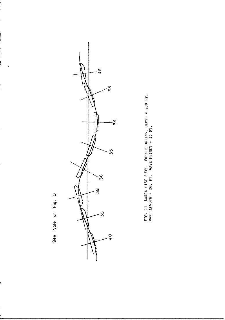
Figure 11 shows the buoy successfully negotiating thL same wave for

the free-floating condition and Fig. 12 sho-3 successful transit

of the moored condition when the wave height was reduced to 30 feet.

A much longer and higher wave is presented in Fig. 15. Figure 13

clearly shows the buoy heaving on the -ave at the natv-Al damped

period of 3.1 seconds, as well as at the period cf the vave.

Water Sheave

Another minor but very interesting investigation made during this

study was that which is sometimes refL.-red to as tho "-iater she Fe"

effect. An illustration of the problem is. say, a mooring in 20,300

feet of water subjected to a 150 kt. wind. At soire tik the wind

suddenly shifts 180 and blows the buoy back along the alignment of

the mooring line unti! it and tne line reach new equilibrium positi,.ns.

How the line tension varies durxng the transient motion has beei. ;

question. It is felt that the form of the line tension colutior

presented here, based on the method of character!stics, is particularly

well suited to handle this problem in a numerical manner.

30

1k s•i,-lar problem as thnt posed above was investigated. How er,

in order to save computer time the top of the line was '.ransiated at .

higher velocity than would be the case if the wind drag only on the

buoy w -c re-rersed First it was determined that if the bucy brokc

free from k1- mioring, a 150 kt wind would pusn it through the water

witb a speed of i13 fps. 'A was decided to translate the line at the

con-.ervativzlY much higher vwlocit) of 25 fps, increasing it linearly

from P fps in the period of 20 seconds. An initial "in ,)lace" or

tens~uned s~.upe of about 1.3 was nssumed and the initiai non-

equilibrium tension oL 7000 !t.s. was established with a iine dia-eter

of 1.5 inches for - ,raterial with &ia-aracteristics as shown in Fig. 3.

The +4rst cumputatioi consisteA of fixing tOe tcp of Lhe line in pacce

and allowing it to reach an equilibrium position. oth positiolus are

shc-n at time equal to zero o-. Fig. "-'. iMen the line was moved to

the left with the velocity function presented above. fhe se-4uential

positions of the line as deteririned by the numerical cemputatior.•

are showr in Fig. 14.

-The tension in the line drc.pped during the first 150 seconds and

then gradually increased until nearly rupturing the line, at which

time the corqut-cions 4ere stopped. During the increase in tension

phase the maximum teiision or.currea at about 0.067 the distance down

the line, The line length changed in accordance with the state of

"-'ension along the line. The tensior, cothtours on the s-t plane are

shown in Fig. 15. It should be noted when examining Fig. 15 that

station 1 represents the anchox and subsequ.ient !; ation numbers are

ipaced 86C.7 feet apart. It can be seen that the tension at the

artc*.or dezrease- for about the first 150 seconds and t)te- steadily

31

increased. Toward the end of the computations the tension in the line

was nearly constant with respect to line position, which *s reasonable

by inspection of Fig. 14.

If the top boune' condition haa been the actual buoy with the

wind onlý driving it, the tensions would have been lower because of the

lower buoy velocity and because of the differences in the initial

loading coidition. When the horizontal component of the line tension

at the buoy had equaled the wind drag of 10,800 pounds the buoy-motion

would stop. Thus it can be seen that the conditions imposed were much

more severe than what would have been experienced at sea. If the

submerged weight of the anchor were less than about 10,000 pounds it

would have been lifted from the bottom (assuming no adhesion to the

bottom) at around 1000 seconds or more. If the real boundary condition

had been imposed at the buoy end, the motion would have been quite

slow and the computer time necessary to complete the problem would

have been prohibitive wizhir. the budget for this study.

Effects From the Environment at Sea

The main purpose of this research was two-fold; 1.) to complete

the debugging of the numerical program and to test it against closed

mathematical solutions, as already discussed, and 2.) to gain sorme

insight into the influence on dynamic line tensions frcm different

wind and currLat loads and •.'ferent line scopes. The work related

to the first item has beer. -resented. For the second purpose it was

decided to design a few moorings in 20,000 feet of water for certain

scopes for a maximum wind condition of 150 kts., subjecting each

mooring to waves of various frequenci-s. Then the same mrorings -ere

tested with the same waves but with a moderate wind velocity of SO kts.

32

The current velocity profiles corresponding to the two wind velocities

are presented in Fig. 2.

As presented previously, the computer program first determined

the steady state, or equilibrium, position of the lines. The f:-,e

different conditions are shown in Fig. 16. in all cases the eqi,ilib-

riunr tension in the line was kept below 47% of the breaking strength

as predicted by Fig. 3. Thus three diameters were selected, as )wn

in Fig. 16. A summary of the load and scope conditions is g;iven in

Table 3.

Two short runs were made in shallow water in order to obtrin a

brief view of the influence of fairly large %aves on line ten!.ion.

The steady load conditions for these two runs are surmnarized in Table

3. The profile equilibrium positions have not been included in a

Figure because they were practically straight lines-

The dynamic program based on the method of characteristics was

compared to the steady state program in terms of the static loads.

The procedure was to assume a water depth of 10,100 feet, a scope of

2.02, diameter of 3 inches, a 100 kt. wind, no wave and a 3urface

current of 6 kts As before, the steady state program determined the

equilibrium conditions, which established the initial conditions for

the dynamic program The dynamic program was then allowed co run to a

7eal time of 65 seconds during which no environmental conditions were

changed. The configuration of the line changed somewhat, but not

beyond what was felt were ac-'ptable limits. It was found that the

angle at the top of the line decreased (which was anticipated because

of the change from equal angle increments to eauai distance increments

along the line) as well as the angle at the bottom of the line. The

33

program ran unzil the angle at the top decreased to a mimimum value,

and then was increasing to when the computations were stopped. The

line tensions were re-distributed somewhat but the total linie length

and the buoy coordinates changed very little. A summary of the

computations is given in Table 5.

It was next desired to subject the five mooring conditions to

waves of various frequencies, or lengths. In each case the wave

height to length ratio was kept constant at 1:15. Thus the waves were

not nearly breaking but also they could not be classified as small

amplitude waves. The dynamic tensions at various stations along the

line were determined and plotted by the computer. Generally. the

m;zimum dynamic tensions occurred at the buoy or at the anchor.

Examples of tensions at the buoy and at the anchor are presented as

Figs. 17 through 32. Point 31A refers to the attachment point at the

buoy. It will be noticed that other frequencies, in addition to the

frequency of the imposed wave, are present. All periods of frequencies

in evidence will be accounted for later.

The computer outpup included tension ccntours in the s-t plane.

Examples are shown for conditions I through V for the 500 feet long

wave as Figs. 33 through 37. The value of each contour line has not

been iidicated but can be determined by the reader by referring to

Fies. 17 through 32. The impoizant thing in Figs. 33 through 37 is

to notice the pattern of line tensions. The nodes of zero or small

tension fluctuations are clearly visible, as are the regions of

maximum tension fluctuations. Equations 33 or 49 can also be used to

approximate the locations of the nodes if the z is replaced with s

That is, the nodes occur where cos ws/a = 0 . A comparison of the

34

results obtained from the numerical model with those from Eqs. 33

and 49 is presented in Table 6. The comparison is fairly good except

at the highest wave frequencies. Thus the position of the nodes can

be estimated from Eq. 33, regardless of the line curvature. This

introduces the possibility of determining the best position for locat-

ing sensitive instrumentation, at least with respect to line position.

That is, the positions of minimum displacement variation can be

determined from Eqs. 31 and 44 by setting sin w- = 0 , or thea

minimum tension variation can be determined by setting cos Ls = 0 ora

the minimum line velocities can be determined from a contour map of

velocities or by taking the total time derivatives of Eq. 31 or 44.

A complete 5ummary of the runs made wiLh waves for conditions

1 through V is given in Tables 7 through 11. Included in the Tables

is the value of the damping coefficient, Q , used, the range, or

double amplitude, oi dynamic tension, the mean value of line tensions

at the end of the iun., the periods of the frequencies evident in the

output records and a calculated line tension based on Eq. 33 for which

the length cf the line was taken as the "stretched" or "in-place"

length at time eoual to zero, and the modulus of elasticity was taken

as that corresponding to the tension in the top of the line at time

equal to zero.

It is desirable to be able to display and compa-e mooring line

tensions in a way that takes into account the difference in line

diameter and length, the differences in wave height and frequency .nd

the resonant frequencies. Thus it is desirable to normalize the

tensions and corresponding frequencies to compare the results of

different types of moorings. The normalizing factor for tensions for

35

this study was based on th)' total saturated ma;s of the line

(excluding the added mass) and a characteristic wave acceleration.

Thus

Normalizing force = v L H w2 (50)

Since eq. 33 can predict the nodes in the line fairly well for the

moorings presente7d here, it was felt that Eq. 34 may suffice for

predicting, at least approximately, the resonant frequencies with

regard to line tensions despite the presence of considerable curvature

in the line. Thus the first modal frequency predicted by Eq. 34 was

used as the normalizing frequency. Conveniently, the first resonant

condition should occur at f/i1 = 1.0 and the subsequent higher mode

resonant conditions occur at f/f. = 2.0, 3.0, 4.0, etc. ThQ resonantI

frequencies of interest for the five conditions are presented in

Table 12. The resulting normalized frequency response curves for

conditions I through V are presented as Fig. 38 for mooring line

tension at the buoy and Fig. 39 for mooring line tension at the anchor.

Admittedly, the data is sparse, but the trend for moorings considered

here is clear. That is, the greatest dynamic response, especially at

the resonant conditions, occurs for the higher wind conditions. The

next most influential parameter is the line scope. It has already

been seen, and is common knowledge, that scope is a most important

parameter for steady state loads. The responses at higher frequencies

tend to bi damped out due to hydrodynamzic action. No data was

obtained for f/f = 1.0 because such a condition would be due to

waves considerably longer than 1GOO feet and such long waves were

uneconomical to consider. However, little energy exists for waves

longer than ISO0 to 2000 feet in most wave spectra.

36

With several curves like Figs. 38 and 39 for a complete range of

water depths, scopes, line dixneters and types, it may be possible to

generate a non-dimensional em.irical solution for dynamic line tensions

for any homogeneous one point mooring. Or perhaps analytical transfer

finctions lased on linear systemas, which are being developed by others,

can be compared to results like Figs. 38 and 39, which consider most

of the non-linearities in the problem. This subject has been left

for future study.

in order to test the program for quite shallow water conditions

and to gain whatever information possible with just two runs, condition

VI for a depth of 150 feet and condition VII for a depth of 1000 feet

were investigated for a wave 600 feet long and 40 feet high.

For the depth of 150 feet the sequential positions of the line

are shown in F.g. 40 from time zero to 13 seconds. At about time

equal to 14 seconds the line tension became negative and the program

stopped because a square root of the negative tension occurs. The

line tension, which was nearly constant along the line at any time is

shown in Fig. 41.

For the depth of 1000 feet the line -emained nearly straight for

all motion. The line tensions again were nearly constant along the

line at any time. The fluctuations in the tension at the buoy and at

the anchor are shown in Fig. 42. It should be recaileti for both

conditions VI and VII that the wind velocity was 50 kts.

3

SUMMARY AND CONSLUSIONS

A review of the basic equations for the numerical modeling of the

mooring line motion based on the method of characteristics and the

motion of the buoy has been made. Solutions for a homogeneous mooring

line have been presented wh,:h include hyateretic damping and hydro-

dynamic damping. In addition, a summary of analytical solutions for

a straight, taut mooring line has been presented and it was attempted

to apply the procedures developed to the single point curved, or less

taut, moorings. It was found that this approximate procedure did

poorly for estimating mooring line tension but did quite well in

estimating the positions of the nodes of tension and in predicting the

natural resonant frequencies of the line.

A new way of presenting frequency response curves for taut or

slack mooring lines subjected to waves was suggested. The normalizing

procedure makes it possible to show the frequency response for lines

of different lengths, diameters and materials on the same scale. Thus

the influence of scope and wind magnitude on dynamic mooring line

tension was presented while normalizing the influence of line diameter.

It was found that smaller scope and/or higher wind increased the

dynamic tensions drastically, as well as the steady state, or mean

line tension.

Two ans were presented for shallow water. It was seen that a

large wave in IS0 feet of water would have been disdstrous to a 2 inch

diameter line, However, the same wave in 1000 feet of water with the

same line and scope produced reasonable dynamic tensions. It was

seen that the tension was nearly constant along the line at any tim•e.

38

Probably a static solution approach would be adeqimte wherein the

line Tension would be determxined based on the sequential positions

of the buoy on the wave and tho subsequent change in scope vithout

regard to accelerations, However, this procedure would be very inade-

quate for deep water maoring-,g.

A presentation of the water sheave problem was made which

illustrated an additional applicat.ion for the numerical przgram.

.. ........

39

.FEERENCES

1. Berteaux, H. 0., "Design of Deep Sea Mooring Lines," MarineTechnology Society Journal, Vol. 4, No. 3, May-June, 1970.

2. Devereux, R., et.al., "Development of An Ocean Data StationTelemetering Buoy," Progress Report GDC-66-093, Convair Divisionof General Dynamics, December, 1966.

3. Felix, M. P., "Hydrodynamic Drag and Frequency ResponseCharacteristics of a Model of a Large Oceanographic Buoy,"Internal Report GDC-ERR-1391, Convair Division of GeneralDyna-mics, December, 1960.

4. Fofonoff, N. P., and Garrett, J., "Morring Motion." TechnicalReport Reference No. 68-31, Woods Hole Oceanographic Institute,May, 1968.

5. Froidevaux, M. R., and Scholten, R. A., "Calculation of theGravity Fall Motion of a Mooring System," Report E-2319,Instrumentation Laboratory, Massachusetts Institute o7 Technology,August, 1968.

6. Goeller, J. E., and Laura, P. A., "Analytical and ExperimentalStudy of the Dynamic Response of Cable Systems," Report 70-3Institute of Ocean Science and Engineering, The CatholicUniversity of America, April, 1970.

7. Martin, W. D., "Tension and Geometry of Single Point MooredSurface Buoy Systems. A Computer Program Study," TechnicalReport Reference No. 68-79, Woods Hole Oceanographic Institute,December, 1968.

8. Mercier, J. A., "Hydro lynamic Forces on Some Float Forms,"Report SIT-DL-69-.1407, Davidson Laboratory, Stevens Institute ofTechnology, October, 1969.

9. Millard, R. C.. "Observations of Static and Dynamic TensionVariations from Surface Moorings," Technical Report ReferenceNo. 69-29, Woods Hole Oceanographic Institution, May, 1969.

10. Nath, J. H., and Felix, M. P.; "A Report on a Study of the Hulland Mooring Line Dynamics for the Convair Ocean Data Stationzelemetering Buoy," Internal Report GDC-ERR-AN-!108, ConvairDivision of General Dynamics, December 1, 1967.

11. Fath, J. H., and Felix, M. P., "A Numerical Model to SimulateBuoy and Mooring Line Motion in the Ocean Environment," InternalReport GDC-AAX68-007, Convair Division of General Dynamics,August 22, 1968.

40

12. Nath, J. H., "Dynamics of Single Point Ocean Moorings of a 8uoy-A Numerical Model for Solution by Cozputer," ProgreS5 ReportReference 69-10, Department of Oceanography, Oregon StateUniversity, July, 1969.

13. Nath, J. H., "An Experimental Study of Wind Forces ol OffshoreStructures," Technical Report CER70-71JhN3, Department of CivilEngineering, Colorado State University, August, 1970.

14. Paquette, R. G., an.' Henderson, B. E., "The Dynamics of SimpleDeep-Sea Buoy Moorings," Technical Report 65-79 Nonr-4SSS(00)to Office of Naval Research, General Motors Defense ResearchLaboratories, Santa Barbara, California, November, 1965.

15. Schram, J. W., and Reyle, S. P., "A Three-Dirmei.sional DynamicAnalysis of a Towed System," Journal of Hydronautics, Vol. 2,No. 4, October, 1968.

16. Wilson, B. W., "Elastic Characteristics of Moorings," Journal ofthe Water Ways and Harbors Division, American Society fTT1Engineers, Proceedings paper 5565, November, 1969.

II1 41

Tfi3LES

I

42

TABLE - COMPARISON BE'PEENi llEiokY AND Ti1E NUMERICAL MODEl. FORLONGI UDINAL DYNAMIC TENSIONS IN A 4T9G.iGhT LINE.

Depth or Variatio- in Lire Tensivn Var-iar.on in Lhi,e t'ensionLinc Length at the Anlchor (lbs) at the Top of the Line

_Num. Model E . 33 Numa. tAfdei Fe.. 33

5,000 L,380 1t330 296 273

10,000 3,2SO 3,200 2,990 2,940

15,000 1,64(- 1,600 990 ý32

20;000 1,7ifl 1,750 1,1;0 1,172

Line diameter = 1.5 inches 6MrA.,us of Elasticity -- 13.1 x 10 pfLine density = 0.02439 slugs/ft (same as sea water)Anpiitude of fcrcing motion = 15 ftFrequency of forcing motion = 0.7 rad/sec

TABLE 2. - COMPARISION BETWEEN NATURALLY DAMPED AND FORCEFOLLY DAMPEDLONGITUDINAL VIBRATIONS FOR A DEPTH OF 20,000 FEET.

Value of the Variation in Line Tens Variation in Line T-asionDamping Coeff., at the Anchor (ibs) at the to'; of the LineQ (1bs)

Num. Model Eq. 33 Num. Model EQ. 33

0 3,237 * 3,677

4x10 2,035 N.A. 2;348 N.A.

Same line and forcing characteristics as for Table 1, c-~•ept.Frequency = 0.610L rad/sec

43

TABLE 3. - SLUMkIRY OF STEADY LOAD LONDITJONS FOR THE FIVE HOORINGS IN20,000 ft. Time 0

Condition Wind Line "Stretched" Tension at Tension atNo. Vel. Dia. Scope Svope Buoy (lbs) Anchor (lbs)

(Kts) (in) I UlT

I 150 3..- 0.80 1.03 99,804 86,614.47 .41A

HI 150 2.5 0.87 1.11 47,777 41,077.44 .38

III 50 2-S 0.87 1.03 16,177 9.32-.1i .09

IV 150 2.0 1.18 1.HC 27,699 23,596.40 .34

V SO 2.0 1.16 1.34 6,983 2,635.10 .94

Note: Scope = Length of line on land water depth"Stretched" scope = Length of line urder load, in place - waterdepth

- -- -----

44

TABLF 4. - SU1JARY OF STEADY LOAD CONDITIONS FOR THE IWO MOORINGS INSHALLOW WATER. Time = 0 Wind Velocity S0 kts

Condition Water Line "Stretched" Tension at Tension atNo, Depth Dia. Scope Scope Buoy (Ibs). Anchcr (Ibs)

(ft) (ins) %b"

vi !So 2 1 32 1.50 2,021 2,001,03 .03

VII 1.000 2 1.32 I.S0 2,564 2,394.04 .03

TABLE 5. - COMPARISON OF EQUILIBRIUM CONDITIONS BETWEEN THE STEADY SIATEPROGRAM AND THE DYNAMIC PROGRAM

Program Time Angle Angle Tension Tension Total X-Coordinate(secs) at at at at Line of Buoy

Buoy Anchor Buoy Anchor Length (ft)(Rad) (Rad) (Ibs) (ibs) (ft)

Steady 0 1.089 0.097 19,977 15,383 24,327 21,531

State

Dynamic 65 0.902 0.021 21,817 12,141 2A,252 21,320

Steady 1.21 4.66 0.915 1.261 1.002 1.010Dynamic

I.- - -

Ac

TABLE 6. COMPARISON OF TENSION NODES BETWEEN THE NUMERICAL MODEL ANDEQ. 33

Wave Node Position from Node Position fromCondition Length Numerical Model Eq. 33

(ft) (ft) (ft)

I S00 4,800 6,920

18,200 20,600 (at buoy)

II 145 4,440 3,680

11,600 11,000

18,900 18,400

32S 5,900 5,500

17,000 16,SCr

SO 6,240 6,800

19,500 20,400

1,000 10,600 9,650

Ili 145 4,800 ? 7,400

10,300 ? 12,300

14,400 ? .7,200

325 3:910 3.690

11,700 11,100

500 5,150 5,150

15.100 15,400

636 S,S00 4,600

16,000 13,800

1.000 7,550 6,450

18,700 19,300

46

TAL .- ContinuedI

Wave Node Position from Node Position fromCondition Length Numerical model Eq. 33

(ft) (ft) (ft)

IV 1S0 4,020 3,730

11,200

17,250 1S,700

275 7,030 5,050

17,400 15,200

S00 8,003 6,800

21,600 2J,400

600 8,350 7,450

23,300 22,300

ISO5 2,510

9,800 7,550

12,500

275 3,400

9,7100 10,200

460 4,450 ?4,360

13,100

500 4,450 4,580

13,700

600 4,450 5.000

10,500 ? 15,000

'40

TABLE 6. Continued

Wave Node Position from Node Position fromCondition Length Numerical model Eq. 33

(ft) (ft) (ft)

IV IS0 4,020 3,730

11,200

17,250 1&,700

275 7,030 5,050

17,400 15,200

500 8,003 6,800

21,600 2J,O00

600 8,350 7,450

23,300 22,300

V 150 2,510

9,800 7,550

12,S00

275 3,400

9,700 10,200

460 4,450 ? 4,360

13,100

S00 4,450 4,580

13,700

600 4,450 5,000

10,500 ? 15,000

00

to 0

00-~ .5- 0

,Ca)

00

V.

000 L

It0

o 0o

m Un

I-n

I I N 0O~ ~48

00 D0 00 0 0* . 00 00 0u 00

CC

*C c 0 _

4~~0 0 U0

co 00 00 0 0

00 00 0

0 0

0 0ý L

im00 CD 0 N 0 000 ouu 0A 0 o-

0.~ 0

0. C-C

00 0000%

tA0 00C 004 00S00 00 100 00;

X. 00o 0* 0 00 00 0

Wn t) C n " 00v 0 0A

0q 0 00

00

hi; CIO..~ '~

00 0000

AA

S ~*O 0 .ýcm,-

a, :; c 0,1~

I~0 0

00c0000? 00

0 00- - ~ 4~Or,

F n '

In In r.,

- II,

IIn

c0 o 'L. 2 -

tt-

00

Io LA is

'L9 0n 0 a

'A c 0 (1q0 0-0 00 cc 0 0000 00 00 00 'A~

00 0Rm In0 n

U In

r.Pt

IC-

SO

zu~ In

li;C) C. Po

aI 00 00 0 0

4ft ~

Boc A-t.

3c~

-~ N **

Sr w0- c O t~

>1 iC 0 0 00 0 0 00

IAI

0

00 0 0 0 0

cc a~ 000 00O~Oa

0o 0

in

in 0'if; t

0000 00 00 00Ci C 00

00 -, V,-t ~ -

00 00027,

00 00 00 0

I' S2

C-4

LU

0 f

lu s- -f -1

00 U4

uIz

0

LU

0..,

oJo

U)-

FIGURES

SVlocui ty

prei I/f-/

FIG- I LIEFIND&JOIN SKI7T2( OF TIE COORiDIrLATE SYTý'

Ve:Dcity ' fps)2 3 4 5 6 7 9-L

50 Knot

"J�Wind

, FW

FM 2 -,31RREN/ VELOCITY DISTRBUTION.

5.0

Trnts Work----- Previous Report, Ref. 12-

A Wilson - Adding 0.1 Strain To His

"Elostic" Curve, Average / J"4.0- of 25 Dio. 8 3" Dio.

13" Strand Nylon /-M ~ 8k -s Plaited Nylon A I

/ -A/

/-

I /1IPermanent

1.2 03 0.4

Strain M% Elongation)

F~r,. 3 STRESS-STRAIN DJAGRAM.

I

I!I

sin w!

FIG. 4 12//!fE VERTIC-A-- --NE

F •bc•!. 4 IDEALIZED VERTICAL ,IN.-.

-'C-

to '

V. U,

10

(spuno) t--U01sua

1 11

~0f=i

(spund Y ioisuaL our

20 '

C Horizontl: Displacement (ft)

FIG. 7 HORIZONTAL LINE DISPLACEMENT FOR ASINUSOIDALLY DISTRIBUTrED INITIAL VELOCITY.

I ____

Numerical ModelHydraulic M1odei(Lr = i: iO

0.5 I Estimated Prototype NaturalPeriod, TdP 2.7 sec.

gI

IiCL 0-

-0 .

-1. 0 I . .

0 1.0 2.0 3.0 4.0 5.0 6.0Normalized Time, t/Td

FIG. 8 NORMALIZED PITCH DECAY CURVE.

Numer:.oall Model"Hydraulic Model

Estimated Prototype Natural

S0.5i Period, Td 3.1 sec-

0

I I__\___,_ --0"5t[

-OO.o 1.0 2.0 3.0

Normahzed T;me, t/Td

FIG. 9 NORMALIZED HEAVE DECAY CURVF.

-0£666!7 .I

0

o 9S66t' ..2

m " --

°- / -

0,"

o E

I~iiL

file

.. •, -o,0

.7

Co.

z 0

c-

14)

00

I, -

0-(

I:~

'C)D

01

00

\W.0 -og

9pogo

'CogJ

O-in

F

-N. -I-rt,9! 0 ,<>

F 1Ua-- ew-r 122

F 808 ..

69t,

00

a R ,o

--Z

0D w

SOS", I U ,1-o 0 C U

00

0C) Or

808

C.I 0

K0 0 U

0 CL

LL o

o I--

o 00

_ j -0

0~0

0 0

S' ~ ~UOIDS w

A Cond. I. Scope = 0.80, Wind = 150 kt. Dia. = 3.S in.

( Cond. iI. Scope = 0.87, Wind = 150 kt. Dia. 2 2.5 in.

O Cond. III. Scope = 0.87, Wind = SO kt. Dia. = 2.5 in.

C' Cond. IV. Scope = 1-18, Wind = 150 kt. Dia. = 2.0 in.

* Cornd. V. Scope = 1.16, Wind = 50 kt. Dia. 2.0 in.

22 ____ ___ I _ _ _ _-_____ _..

20F

181

on ib[-

o 14

~ / //0C. 81- -

S6.o4

II2!-

0 2 4 6 8 10 12 14 16 18 20 22 24

x Distarnce from Anchor x 10- (ft)

FIG. 16 EqU.LIBRIUM POSITIONS FOR VARIOUS KcJJRING CONDITIONS STUDIED.

rI4.-,

I

-.- *..- .m.�J4== -� -�--

4-

It *

- - - - - - - - -- a * .4 - -- a a - - - 0 * * N

* * -4

I

.t----- '-': ' , .. . .- '" :

t ! I ! __L - -- - •

, I I 1 "'-•

I- F

___

- 3S*)i*i -:

�I.

ISS.nt&thu zI � � �

- t - - -

4-,

� - -�

- - e a - - -*4 - - - -, - - - - - C- a - -C - a.4 .4 .4 = .4 *t

z

C,4;

II

II

C-

C,'

II

C-

� II __

0

zC

C

7__ -�

C-

.1- a a a - - a- - - - - - - - - 0o - C - a - - -.* 0 4 0 - - 0 4 -* a S S 4 5 5 4 1

z

0rN*.

WSWa

................................ I

.........

. . . .------

tn

I

r -

'�1

I,.,isr

-- s,.1,,i. *

F �a.3av

V -

I.U

I ------*--1* *_Ii. _-I. -J

_________________________________ I _________________________________

- - Cd - - Cd- - - - - - - z

* a - - a -* a - - 0

ci,�, I?�2� z

I')

r'a

II

L..

III * 1 I '-4

- � I I7K r�fl II �.* �

* I -4-�---I-----$4�Ie �

LL.

01 - If)

I- I.33t:I I, I

II -

- tS.Ifl0

_

I-

z$

a - - a - C

- * S C 7 - aS S - C C C -, C

,flI11

2

11 T4111*

It-ost

0n

Li'!12

IDMs'

CLL

$-lost

- w

IL

IIW

t4)

t: t

456

L-15

* 0

______1777135a. .

-LLZ

-F-

tonl

00

_______________________ I_____________________

II

L.

II

* w

V ____ ____

It

Hi'.. _

?u.2901I V _

I - -I 0

_______ 1-4

�,. �1,.z0U

Es * 312'*

9

- -

wI-.

St S a S a -- a - -* * * S- - - * - - z- - - - - - 0o - a - St

- - - -

'iCI�b

LLU

to-loW

L,.

SO I 19ff~jil0

0P

FII

td�

II

- -r

* LL

I _ __ tf�

I.... * * .*

1* 3.,-

KI:-t ____ ___ ___ ____ ____

___ ____ I...

- - - - - - - zL74* 4 - aI.-

%�S�3.

(2

LLI

* - -. -33. 1

-~~ . . . . . ... . .

II

L.�A.

--.-----

-. - ---- �=�--�-- a-- I-

- - .' - --- ___ - � -��----- -

- �-=z-...... -. - - -- --- ,- - - - - a a s131.. � W

- � �-:-----... .f¾.-� - - - .............................................

- - :�-:�� - - ..z a a- - ---

- ----- =---.. ------------ - -�. ... *- - - :

-� . I-- -- a- - -�-� -

- - - - - .......- a: £S.?.t. .�- 0-- .'. - -. . . 0

- . - -a---- - *%-

- -� . s,.1u.. -

* i.�---� - -

__ - - a a £*36.. :- Z

* * -. a.-. - .- * a � $s.Iss.-

.�

-a- u.-.

- -.- : - - -. -. - -

-- I a .a - *�-:. -

- . * - .

: w - - - .- * �-- - - �- IL j�.2e:9�� -

-: - . - - - . - * u�3::i- -- - --- 7:

- -� 4a a--- . -.'a a-.---

- ..

- -� � a a .z- - - Z�. � I 1 t:.Z::t 8 0

* - .. z'a'

- - - e:-J" .-- �..

1 1-. I I I I I I J......j...,.X...J.... , I J-..�..-.-. - *4 - N - - '4 *4 A� *4 *4 *4 *4 *4 *4 a. *j e -. - -

- a a a a C a a a *. .. .. *. -. -

ta - - - - - �.4 - - - �. - - - - - - -S 0 C - - - S aS n... .

- * 0t- .0. *4 - N - - * - - .. .. - ....a - *4 *4 *4 *4 - *4 *4 *4 *4 � a - . .0 0 *4 - *4

F-

1? A I A~ -1 1 ' ' -_______ _____ 4

7---z- -- -- -

-- ~--- ~ - - .----'.- - - - - - - - - - -- -

. . . ..- . . . . . -. . . . . 1

- - -

C.:.

•. -- :.,-- -. . . £. 3att _A.. -"-'"-~ -.- £1.1,. . •

-- . .- . . -

-.--- .2 .: .. . -- . ... - ..-:•.-- . .

1 4 ' .- z4--- ~-t; -i I

- . . ..-.- -"-=' -- .-• • - Sl. 3S.. 1-]1 .

. . . .. . . . . . . . .- _ .. . .- ..

-.. . . . -- -- . .. . " - 5I-.3l1 '

*. .. . *,. , *

.. .. .. ....................... ~- 7_-**3, -

- . - 4. w. . . .- . . . . . -

. . .. . - -

.. . . . . . . . . . ...... ...-. •% .•• ,. •. . ,. .

- . . . . . . u. o .- .o

-- "Z-

- --

- ~ ~ o ft~4:~

0 I

/ 0

LU

0i

w l

-. \OZ~

d ~.

H~~~~ ~ ~ ~ -1T>U'Sa slolta ''4 z

IiII 0z

U* 0

F- 0

V.,

-- 40-

V o r- ( t 7 rI-S~. souluw(

II

200 : ,

kTime Sequence, seconds

,69 -0 I0,'60r 7~ Z I

140 0 12

120"7' - 7

100

so-Net aL I ! •40 4

20 40 60 80 100 120 140 160 180 200 220 240x (ff)

FIG. 40 SEQUENTIAL POSITIONS OF THE MOORING LINE. DEPTH =1SO FT. WAVE LENGTH = 600 FT. WAVE HEIGHT = 40 FT. WIND SO KTS.

7Ultimate Tension7.0; I r ' ---- -3--- -

6.0 Line Diameter 2 in.

5.0

4.0

~3.0-

2.4

iOlLot.. __ _ _ _ _ _ _ _ _ _ _ _ _ _ _

0 2 4 6 8 10 12 14 16 18Time (seconds)

FIG. 41 •NOORINGS LINE TENSION. DEPTH iSO FT. WAVELENGTH 600 FT. WAVE HEIGHT = 40 FT. WIND = 50 KTS.

STension at Anchor

5k S _ Tension at Buoy

Line Diameter 2 in.

S4--

* I!

0 10 2 0 4 0 6 7 0 9 0 1

b 'I

_ v~~ I I !

*- ,I I,, II

SI I4I I i l I'

!0 I0 20 30 40 50 6 70 8 90 I0 I1

Time (seconds)

FIG. 42 MOORING LINE TENSION. DEPTH = 100 FT. WAVELENGTH = 600 FT. WAVE HEIGHT = 40 Ff. WIND = SO KTS.