Frugality Is Hard to A�ord

A.Ye³im Orhun and Mike Palazzolo ∗

Abstract

Households commonly utilize strategies that provide long-term savings on everyday

purchases in exchange for an increase in their short-term expenditures. They buy larger

packages of non-perishable goods to take advantage of bulk discounts, and accelerate

their purchases to take advantage of temporary discounts. Even though low-income

households are more incentivized to save, they are less likely to take advantage of these

money-saving strategies. We provide causal evidence that liquidity constraints inhibit

low-income households' ability to do so.

∗A. Ye³im Orhun (aorhun@umich.edu) is Assistant Professor of Marketing, Ross School of Business; 701Tappan Street, Ann Arbor, MI, 48109. Mike Palazzolo (mpalazzolo@ucdavis.edu) is Assistant Professor ofMarketing, UC Davis Graduate School of Management; One Shields Avenue, Davis, CA, 95618. Authororder is alphabetical. The authors wish to thank Dan Ackerberg, Rajeev Batra, Stephanie Carpenter, FredFeinberg, Linda Hagen, Tom Kinnear, Aradhna Krishna, John Lynch, Kanishka Misra, Jenny Olson, BeatrizPereira, Eric Schwartz, S Sriram, the marketing faculty at the Leavey School of Business, and the attendeesof the 2016 Boulder Summer Conference on Consumer Financial Decision Making for their assistance andsuggestions. We are grateful to the Kilts Center for Marketing at Chicago Booth for providing us with thedata. A.Ye³im Orhun gratefully acknowledges research funding provided by the 3M Company.

1

Introduction

Households have several strategies at their disposal to reduce per-unit spending on ev-

eryday products. One set of strategies o�ers consumers immediate �nancial savings, such as

buying cheaper, lower-quality brands or searching for lower prices. In line with the intuition

that individuals who have the greatest incentive to save money should be most likely to use

these strategies, past research has shown that lower-income households purchase cheaper

brands (Ailawadi, Neslin, and Gedenk 2001; Akbay and Jones 2005; Gri�th, Leibtag, Le-

icester, and Nevo 2009; Kalyanam and Putler 1997) and make more of an e�ort to search

more for lower prices (Aguiar and Hurst 2005) than their higher-income counterparts.

A second set of money-saving strategies o�ers long-term savings in exchange for an in-

crease in short-term expenditure. For example, households may purchase larger packages

to take advantage of bulk discounts that o�er a lower per-unit price. Similarly, house-

holds may accelerate their purchase of a given product when they �nd an attractive deal.

These intertemporal substitution strategies are commonly used for everyday purchases of

non-perishable goods. However, low-income households are likely to face higher liquidity

constraints that may inhibit them from increasing short-term expenditures. Therefore, these

households may fail to utilize intertemporal money-saving strategies to their full potential,

even though they have strong incentives to save.

The main objective of this paper is to test whether liquidity constraints inhibit the

ability of low-income households to (1) buy in bulk and (2) accelerate purchase timing to

take advantage of sales. We quantify the extent to which liquidity constraints, as opposed to

other possible limitations (e.g., storage constraints, limited access to channels that provide

bulk options, �nancial illiteracy, less price information if they visit stores less often, consumer

myopia), inhibit low-income households from utilizing money-saving strategies that require

up-front investments. To this end, we employ time of the month as a liquidity shifter for

low-income households and compare (1) the di�erence in low-income households' tendency

to utilize money-saving strategies that require up-front investments at the beginning and

2

end of the month with (2) the di�erence in higher-income households' tendency to utilize

these strategies at the beginning and end of the month. This approach is motivated by

the notion that low-income households are likely to be the most liquidity constrained later

in the month, because they are more dependent on cash in�ows that accumulate earlier

in the month and are depleted as the month goes on. By contrast, middle- to high-income

households are less likely to be cash constrained for basic necessities at any time of the month.

Because we are examining within-household di�erences in purchase behavior across time,

our empirical approach identi�es the impact of liquidity constraints on purchase behavior,

above and beyond the impact of any household-speci�c and time-invariant factors. We

also demonstrate that our conclusions are robust to potential variations in the availability,

a�ordability, or desirability of products and channels that may be systematically correlated

with time of month.

Our analyses are based on purchases of more than 113,000 households over nine years

in the toilet paper category. The toilet paper category is suitable for studying consumers'

intertemporal substitution strategies for the following reasons. First, bulk and temporary

discounts are both common in this category. Second, toilet paper is storable, and therefore

bulk buying and accelerating purchase incidence to take advantage of sales are both plausible

money-saving strategies. Third, a household's need for toilet paper cannot be satis�ed

by other product categories; therefore purchasing behavior in this category is unlikely to

be in�uenced by substitution to or from other categories. Finally, the simplicity of the

attributes of products in this category allows us to pool our analyses across products using

a standardized unit of toilet paper.

The paper proceeds as follows: In the Related Literature section, we discuss relevant pre-

vious research and delineate our approach and contribution. In the Data section, we describe

the data and document cross-sectional di�erences in the propensity to utilize intertemporal

saving strategies across households of di�erent income groups. We show that lower-income

households are less likely to utilize money-saving strategies that require up-front invest-

3

ments than households with higher-incomes. Why are consumers with the greatest incentive

to save the least likely to employ intertemporal money-saving strategies? In the Empiri-

cal Analyses section, we show that low-income households would utilize these money-saving

strategies more often, even in the presence of other money-saving opportunities, if they had

greater liquidity. Speci�cally, we �nd that when their liquidity constraints are partially

relaxed, households making less than $20,000 are able to close at least 3-4% of the bulk

buying gap and 100% of the purchase acceleration gap relative to the purchasing practices

of the highest-income households. We o�er several robustness checks and related discourse

in the Discussion section. In the Conclusion section, we review the potential implications

for retailers and policy makers.

Related Literature

This paper investigates the extent to which liquidity constraints inhibit low-income house-

holds' ability to utilize two common intertemporal money-saving strategies: bulk buying and

purchase acceleration. Our work draws from and contributes to the literature on (1) the var-

ious �nancial burdens shouldered by the poor (the �poverty penalty�) and (2) the impact of

liquidity constraints on spending.

Related research on the poverty penalty can be broadly classi�ed into three streams. The

�rst stream aims to document cross-sectional di�erences in the prices that di�erent income

groups pay to receive similar services or products. Most applicable to this paper, several

researchers (Attanasio and Frayne 2006; Beatty 2010; Frank, Douglas, and Polli 1967; Gri�th

et al. 2009; Kunreuther 1973; Rao 2000) have investigated whether households from di�erent

income groups di�er in their propensity to purchase in bulk, which a�ects the per-unit prices

they pay. The second stream of research documents the ways in which low-income households

are disadvantaged by their shopping environments. For example, these households live in

areas where retail competition is sparse, retail costs are high, and large supermarkets are

absent or hard to get to, which leads them to pay higher shelf prices (Kaufman et al.

4

1997; Chung and Meyers, 1999; Talukdar 2008). The third stream of research investigates

the extent to which di�erences in household resources, rather than shopping environments,

contribute to the poverty penalty. This paper contributes mainly to the last of these research

streams, as our primary objective is to investigate how liquidity constraints a�ect low-income

households' choices within the shopping environment these households face.

Research in this third stream has investigated several resource constraints that may

inhibit households from taking advantage of money-saving opportunities, even when those

opportunities are available in their shopping environment. For example, Aguiar and Hurst

(2005) show that consumers with a higher opportunity cost of time are less likely to engage

in price search and thus pay higher prices. Talukdar (2008) shows that a lack of access

to transportation inhibits low-income households from engaging in price search as much as

higher-income households. Bell and Hilber (2006) show that consumers with greater storage

constraints (smaller-sized residences) shop more often and purchase smaller quantities. Other

researchers have found that the attentional demands of poverty reduce the cognitive resources

of the poor (Mani et al. 2013) and that low-income households may be more myopic or

present-biased (Delaney and Doyle 2012; Griskevicius et al. 2011). Because intertemporal

money-saving strategies require planning for the future, the results of these studies suggest

that lower-income households may be less able or less inclined to utilize these strategies,

even when they are available. Finally, liquidity constraints can a�ect low-income households'

ability to make immediate investments for future gains.

The limiting e�ect of liquidity constraints on lower-income households' ability to take

advantage of money-saving strategies that require up-front investment is perhaps intuitive.

Indeed, earlier work has speculated that liquidity constraints may be a driver of cross-

sectional di�erences in the propensity to buy in bulk (Gri�th et al. 2009; Kunreuther 1973).

However, previous work does not formally test for a relationship between liquidity constraints

and bulk buying. The empirical literature studying purchase acceleration (Erdem, Imai, and

Keane 2003; Hendel and Nevo 2006; Neslin Henderson, and Quelch 1985) does not provide

5

any evidence that households of di�erent income levels di�er in their utilization of this

strategy, nor does it study the role of liquidity constraints. Therefore, empirical evidence of

a relationship between liquidity constraints and these intertemporal money-saving strategies

is lacking.

Macroeconomics literature has studied how total spending may be impacted by large, one-

time shifts in wealth, such as economic stimulus payments (Broda and Parker 2014; Misra

and Surico 2014; Parker et al. 2013) and tax refunds and rebates (Agarwal, Liu, and Souleles

2007; Bertrand and Morse 2009; Johnson, Parker, and Souleles 2006; Johnson, Parker, and

Souleles 2009; Shapiro and Slemrod 1995; Souleles 1999). It has also examined how a

household's ability to purchase expensive, durable items, such as automobiles (Attanasio,

Goldberg, and Kyriazidou 2008; Benmelech, Meisenzahl, and Ramcharan 2015) and houses

(Engelhardt 1996), is a�ected by such shifts. Other researchers investigate the impact of

smaller but recurring shifts in income, such as the receipt of paychecks (Stephens 2006; Zhang

2013), food stamps (Beatty and Tuttle 2014; Hastings and Shapiro 2017), or Social Security

checks (Stephens 2003) on household spending. Our work di�ers from this literature insofar

as we examine individual households' propensity to utilize speci�c money-saving strategies,

rather than merely quantifying changes in their total spending.

Relatedly, Nevo and Wong (2014) and Dubé, Hitsch, and Rossi (2015) recently investi-

gated how households' propensity to purchase private labels and redeem coupons was a�ected

by large changes in wealth during the Great Recession. However, both the particular money-

saving strategies and the type of liquidity shifter we study are di�erent from those examined

in these papers. First, we focus on money-saving strategies that require an increase in up-

front spending. Second, we utilize a partial but recurring relaxation of liquidity constraints

for low-income households, proxied for by the in�ux of cash they receive at the the begin-

ning of the month. Using recurring �uctuations in liquidity instead of large, one-time shifts

in wealth provides important advantages for our research. First, recurring �uctuations are

easier to disentangle from unobserved factors because they are not one-time events. Second,

6

they do not create structural changes in a household's behavior as, for example, the pur-

chase of a car might. Third, the results are likely to be more relevant for common policy

interventions (e.g., food stamps) that provide small, recurring infusions of liquidity.

Data and Cross-Sectional Patterns

For our analyses, we use the Nielsen consumer panel data for the years 2006�2014, pro-

vided by the Kilts Center for Marketing at the University of Chicago Booth School of Busi-

ness. This data set contains all purchases by participating households during the period

for which they were members of the panel.1 For each purchase occasion, the data provide

the retail channel shopped in; the price, quantity, and package size of each UPC (Universal

Product Code) purchased; an indicator for whether each UPC purchased was on sale; and

the purchase date.

Our analyses focus on the toilet paper category. In this category, there are many oppor-

tunities to save. Brands vary considerably in their prices, and bulk and temporary discounts

are common and substantial. Table 1 documents price variation and illustrates the mag-

nitude of bulk discounts by comparing prices across major brands and sizes.2 In general,

the brands that have relatively low everday prices o�er shallower bulk discounts and are

purchased on sale less frequently.3

[Insert Table 1 about here]

1A well-known limitation of the data set is that there are some notable recording discrepancies apparentin the raw data. Some listed package sizes are clearly erroneous (e.g., one UPC was reported to contain 1,296rolls of toilet paper). In addition, a few households seem not to have reported all their purchases (e.g., forsome households, several years elapse between reported purchases). Einav, Leibtag, and Nevo (2010) notethe importance of accounting for potential recording discrepancies in the Nielsen data set. We therefore makea conservative e�ort to clean the data, correcting or removing entries that su�er from severe and obviousdiscrepancies. We retain 91% of observations for our analyses, and our conclusions are not sensitive to theremoved entries. We provide a detailed description of our cleaning approach in the Online Appendix.

2The most commonly purchased package sizes are 1-, 4-, 6-, 9-, 12-, 24-, 30-, and 36-roll packages, whichtogether account for 91% of purchases. The top �ve brands (Angel Soft, Charmin, Kleenex, Quilted Northern,and Scott) account for 73% of purchases, and private labels account for another 20%.

3We describe each product by the number of standardized rolls it contains to facilitate more accuratecomparisons across products, as rolls may di�er in ply and the number of sheets they contain. We use 275sheets of two-ply toilet paper as the standardized unit, as it re�ects the average number of two-ply sheetsper roll in the UPCs in our data set. Unit prices are also measured in terms of standardized rolls.

7

In total, the panel data set contains more than 113,000 households that purchased in the

toilet paper category. These households made a total of 3.2 million purchases from 2006 to

2014 in this category, primarily at grocery stores (47% of purchases), discount stores (29%),

warehouse stores (8%), drug stores (6%), and dollar stores (6%). The average household

purchase pattern indicates a consumption rate of slightly less than a roll of toilet paper

per capita, per week. Based on households' yearly income levels reported in the Nielsen

data, we sort households into �ve annual household income groups that closely mirror the

income quintiles in the United States. Speci�cally, we con�gure income groups as follows:

Income Group 1 = <$20K, Income Group 2 = $20K�$40K, Income Group 3 = $40K�$60K,

Income Group 4 = $60K�$100K, and Income Group 5 = >$100K.4 Table 12 in the Appendix

presents some basic statistics about other household demographics.

Previous research has established that low-income households are more price sensitive

(Ailawadi, Neslin, and Gedenk 2001). Therefore, we expect these households to have greater

incentives to save. Table 2 suggests several ways to save in this category. Households can

save by purchasing cheaper brands, by purchasing larger package sizes, and by timing their

purchases to take advantage of temporary discounts. In our preliminary analyses presented

here, we ask how households of di�erent income groups di�er in their propensity to take

advantage of these strategies. Previous work has found that low-income bouseholds are

more likely to buy cheaper brands, such as store brands (Ailawadi, Neslin, and Gedenk

2001; Akbay and Jones 2005; Gri�th, Leibtag, Leicester, and Nevo 2009; Kalyanam and

Putler 1997). To check whether these cross-sectional di�erences also hold true for our data

set, we perform the following cross-sectional regression:

Yhtp = β1 +∑5

i=2 βiI[INCht = i] +∑3

j=1 µj[Consumption]jh + εht

The binary variable (Yhpt) either indicates whether purchase p made by household h dur-

4Actual quintiles in 2011 were $0�$25K, $25K�$45K, $45K�65K, $65K�105K, and >$105K (seehttp://en.wikipedia.org/wiki/Household_income_in_the_United_States). The income buckets used byNielsen, though fairly granular, do not allow for groupings that perfectly match these quintiles. Comparedto the national income distribution, the panel data set provides fairly good coverage of each income group,although it slightly overrepresents the middle-income groups.

8

ing trip t was (1) the cheapest brand in the household's designated market area (DMA), given

the size purchased, or (2) a store brand.5 The income group dummy variable, I[INCht = i],

is equal to 1 if household h is a member of income group i during the year of purchase, where

i = 1 corresponds to households with incomes less than $20K, i = 2 corresponds to house-

holds in the $20K�$40K income range, i = 3 corresponds to households in the $40K�$60K

income range, i = 4 corresponds to households in the $60K�$100K income range, and i = 5

corresponds to households with incomes higher than $100K. A third-order polynomial of

the household's average consumption rate, [Consumption]h, controls for heterogeneity in

shopping behavior that is driven by di�erences in consumption rates that may otherwise be

attributed to di�erences in income.6

[Insert Table 2 about here]

The results in Table 2 show that households in the lowest-income group are the most

likely to choose lower-priced brands. For example, compared with households in the highest-

income group that have a similar consumption rate, households in the lowest-income group

are 10% more likely to buy store brands and 4% more likely to buy the cheapest brand

of a given size. In contrast, low-income households are less likely to save by purchasing

large packages. The last column of Table 2 reports the results of regressing the package

size purchased (in standardized rolls) by household h during trip t on the same explanatory

variables. The results suggest that low-income households purchase UPCs containing 4.64

fewer standardized rolls than higher-income households with similar consumption rates.7

5The Online Appendix provides details of how we identi�ed the cheapest brand, and presents resultsfrom alternative de�nitions of the cheapest brand at both the DMA and DMA-channel levels. Lower-incomehouseholds are more likely to buy the cheapest brand, regardless of how it is de�ned. The Online Appendixalso presents cross-sectional di�erences in coupon usage. Lower-income households are less likely to usecoupons, in line with previous �ndings of the literature (e.g., Bawa and Shoemaker 1987).

6We detail the calculation of consumption rate in the Online Appendix. We use a polynomial to avoidassuming a strictly linear relationship between consumption and size purchased. Without consumptioncontrols, the cross-sectional di�erences between income groups are larger.

7Some of the previous work examining cross-sectional di�erences in bulk buying has also found thatlow-income households are less likely to purchase larger-sized packages (Attanasio and Frayne 2006; Frank,Douglas, and Polli 1967; Kunreuther 1973; Rao 2000). Others, however, have reached the opposite conclusion(Beatty 2010; Gri�th et al. 2009).

9

Because low-income households are more price sensitive than other households, they

would presumably want to utilize all money-saving strategies available to them to the same

extent as, if not more so than, higher-income households. It is important to note that

di�erent money-saving strategies are not mutually exclusive options. All brands in this

category are available in bulk, therefore households do not have to choose between buying

cheaper brands and purchasing larger package sizes. It is puzzling, then, that they use

one money-saving strategy (buying cheaper brands) more than other households, but use

another strategy (bulk buying) less. This is made all the more puzzling by the fact that the

potential savings from buying in bulk are quite substantial, even for the brands low-income

households prefer. The data suggest that low-income households could save an additional

8.8% per standardized roll if they purchased larger sizes of the brands they prefer at to the

degree that the highest-income households do. Importantly, these foregone savings are in line

with the savings they accrue by purchasing cheap brands. Purchasing cheaper brands than

the highest-income households saves these households 9.6% per standardized roll compared

to what they would pay if they purchased the brands the highest-income households did.8

The potential savings available from buying in bulk and buying cheaper brands are generally

comparable, even at the extremes. Low income households could save an additional 21.7% by

always purchasing the largest package size available, while keeping their brands purchased

the same. They could save 24.6% by keeping by always purchasing the store brand, but

keeping their package size purchased the same. These numbers convey that low-income

households could achieve signi�cant savings, comparable to the levels that other savings

strategies provide, if they purchased larger package sizes. Therefore, low income households'

tendency to buy in bulk less than higher income households cannot be a consequence of

insu�cient savings o�ered through bulk discounts for the cheaper brands they prefer.

What, then, could explain the gap between low- and high-income households' propensity

8Note that our calculations of savings along the package size and brand dimensions are done holding theother dimension constant. The Online Appendix provides details on how we calculate the savings numbersreferenced in this section, provides a full set of comparisons between all income groups rather than just thelowest- and highest-income groups, and provides a more thorough discussion for the interested reader.

10

to buy in bulk? The literature has speculated that several factors could contribute to this

gap, including lack of transportation, lack of storage, lack of access to stores that carry bulk

items, lack of �nancial sophistication, and liquidity constraints.9 This paper examines the

liquidity constraints hypothesis�that low income households may not buy in bulk as much

as they would like to because they cannot a�ord the increase in up-front expenditure buying

in bulk requires.

If liquidity constraints inhibit low-income households from taking advantage of money-

saving opportunities that require an increase in up-front expenditure, we would also expect

low-income households to be less likely to accelerate purchase incidence to take advantage

of temporary discounts. As Neslin, Henderson, and Quelch (1985) and Hendel and Nevo

(2006) point out, if a household is buying earlier than it otherwise would (i.e., accelerating

its purchase timing) to take advantage of a sale, then the household's average interpurchase

time preceding sale purchases should be shorter than the household's average interpurchase

time preceding non-sale purchases. To check whether households from di�erent income

groups di�er in their propensity to accelerate their purchase timing to take advantage of

sale, we evaluate whether the di�erence between sale and nonsale interpurchase times is less

pronounced for low-income households than for high-income households with the following

regression:

IPThtp = αh + δhI[sale]htp +∑5

i=2 νiI[INCht = i] + εht

where δh = δ1 +∑5

i=2 δiI[INCht = i] +∑3

j=1 µj[Consumption]jh. Here, we regress the

interpurchase time preceding a purchase, IPThtp, on household �xed e�ects, αh, to account

for households' baseline interpurchase times; an indicator for whether the purchase was

made on sale (I[sale]htp); and its interaction with the household's income group and with

the third polynomial of the household's consumption rate, to test for income-level

heterogeneity in the interpurchase time response to sale, while controlling for systematic

9In the Appendix, we report changes in our cross-sectional estimates across multiple speci�cations thatinclude controls for geographic access and other household characteristics for the interested reader. Theseresults are consistent with past research.

11

di�erences in consumption across households. The regression also includes household

income group dummies to account for variations in household income over time. Table 3

shows that the estimate of δ1 (the baseline coe�cient for I[sale]htp is negative suggesting

that for low-income households, the length of time between a sale purchase and a

household's previous purchase is shorter than the length of time between a nonsale

purchase and a household's previous purchase.10 This result is consistent with �ndings in

the previous literature (Neslin, Henderson and Quelch 1985; Hendel and Nevo 2006).11

Moreover, the estimates for all higher-income groups (δi for i > 1) are negative and

decreasing, indicating that higher-income households accelerate their purchase timing even

more than low-income households do.12 Speci�cally, the interpurchase time for low-income

households' sale purchases is only 1 day shorter than that for their non-sale purchases,

while the di�erence for the highest-income households is 2.5 days.

[Insert Table 3 about here]

The results of our cross-sectional analyses provide evidence that low-income households

utilize intertemporal savings strategies less often than higher-income households do. These

�ndings are consistent with previous research that found similar cross-sectional di�erences

in bulk buying behavior. Why do the households with the strongest incentives to save utilize

these money-saving strategies the least? In the empirical analysis that follows, we depart

from prior work by testing whether and to what degree liquidity constraints inhibit low-

income households from utilizing money-saving strategies that require up-front investments.

10Note that not all sale purchases involve acceleration; at times, households are planning to buy and, bychance, happen to �nd a sale on the same day. These estimates should therefore be interpreted as lowerbounds on the magnitude of purchase acceleration, as the parameter estimates measure the average di�erencebetween sale and nonsale interpurchase times, regardless of whether a sale purchase was due to accelerationor not.

11Similar to this previous literature, we also present results showing that the interpurchase times after salepurchases are longer than interpurchase times after nonsale purchases (Appendix, Table 14). The resultssupport the notion that households are not merely buying earlier to consume more in the current period,but are storing for future consumption.

12To the best of our knowledge, the only previous research to test for purchase acceleration di�erencesbetween income groups, Neslin, Henderson, and Quelch (1985), did not �nd any signi�cant di�erences,potentially due to a much smaller sample (N=2,293). The sample size is important to identify di�erencesacross income groups because the within-household variance in interpurchase times is quite large.

12

We detail how our empirical strategy isolates the impact of liquidity constraints on low-

income households' propensity to use these strategies from the impact of other potential

limitations in household resources (e.g., storage constraints, geographical access, myopia,

�nancial illiteracy).

Empirical Analysis: The Role of Liquidity Constraints

Identi�cation Strategy: Liquidity Shifter for Low-Income House-

holds

Our central hypothesis is that liquidity constraints inhibit low-income households from uti-

lizing intertemporal money-saving strategies as much as they would if they were uncon-

strained. Because we cannot experimentally vary the cash reserves of low-income households

directly, we instead rely on a proxy that is generally associated with higher liquidity for these

households: the beginning of the month. Speci�cally, our di�erence-in-di�erences analyses

compare (1) the di�erence in low-income households' tendency to utilize these strategies in

the beginning of the month versus other times throughout the month with (2) the di�erences

in higher-income households' tendency to utilize these strategies across the span of the same

time periods. Because we expect liquidity constraints to be binding only for low-income

households when it comes to low-priced, everyday goods like toilet paper, we expect to ob-

serve larger di�erences in purchase behavior at the beginning versus the end of the month

for low-income households than for other households.

Two important features of the di�erence-in-di�erences analysis are worth highlighting.

First, inferences are based on within-household variation in purchase behaviors. There-

fore, inherently household-speci�c and time-invariant di�erences across households, such as

storage constraints, transportation constraints, access to di�erent stores, myopia, or �nancial

literacy are controlled for and do not confound the estimates of interest. Second, because sys-

tematic di�erences in the shopping environment from week to week (e.g., perhaps temporary

13

discounts for bulk sizes are more common during the �rst week of the month) are available

to all households that shop in that environment, di�erences in the estimates of households'

reactions to liquidity relaxation are not contaminated by such �uctuations. In the Discus-

sion section, we provide additional analyses to show that controlling for time variation in

the shopping environment or in the desirability of options does not a�ect our conclusions

and that our assumptions for the di�erence-in-di�erences approach are appropriate.

Admittedly, each low-income household has its own unique cash-�ow schedule, and thus

there is great variation in liquidity across households at any given time of the month. Pay-

ments (e.g. earnings, Social Security payments, food stamps) may arrive at di�erent times,

and spending patterns �uctuate as well.13 Therefore, the beginning of the month is a noisy

instrument, and our results should be treated as conservative (as we detail further in the

Discussion section). However, the proxy is valid as long as it exogenously shifts liquidity

availability for low-income households. Both previous research (e.g., Stephens 2003) and

the shopping patterns re�ected in the Nielsen data indicate that low-income households are

more likely to have higher liquidity at the beginning of the month. Previous research has

shown that households respond to temporary increases in liquidity by increasing their total

spending (Stephens 2006; Zhang 2013). Consistent with this, the low-income households in

the Nielsen data experience signi�cant increases in their average daily expenditures early in

the month, but the high-income households do not. For each income group, Figure 1 dis-

plays the percentage deviation of the group's average daily trip incidence and expenditure

from the group's average monthly pattern of trips and expenditure, for all categories (in the

left panel) and the toilet paper category (in the right panel). For all categories, the �gure

shows a clear decline in propensity to shop and daily expenditure for low-income households

over the course of the month, a more modest decline for the second income group ($20�$40K

annual salary), and virtually no change for the other income groups once patterns that a�ect

13Social Security payments are usually distributed on the last day or the �rst week of the month. Most ofthe low-income households in our panel live in states where the distribution dates for food stamps correspondto the beginning of the month. Finally, monthly or bi-weekly paychecks also boost liquidity at the beginningof the month.

14

all income groups are accounted for.14 For the toilet paper category, low-income households'

shopping propensity and spending per trip is highest in the beginning of the month and

sharply declines over the rest of the month, whereas the trip incidence and spending pat-

terns of households making more than $40K are fairly stable across the month. Note that the

change in the second income group's behavior is much less pronounced in the toilet paper

category, possibly because these households do not feel as constrained for purchases with

such a low price point.15 Therefore, while in general time of the month may impact the

liquidity of the second income group, we expect the proxy to impact primarily the purchase

behavior of the lowest-income group in the toilet paper category.

To provide a robust set of analyses, we employ �ve di�erent liquidity shifters. Each

measure is a dummy variable indicating whether the purchase was made at a time of relatively

high liquidity. The �ve measures correspond to the following conditions: (1) the purchase

was made during the �rst week of the month, (2) the purchase was made during the �rst

week of the month and on the household's �rst trip to a store that month (to purchase from

any product category), (3) the purchase was made during the �rst week of the month and on

the household's �rst or second trip to a store that month, (4) the purchase was made during

the �rst ten days of the month and on the household's �rst trip to a store that month, and

(5) the purchase was made during the �rst ten days of the month and on the household's

�rst or second trip to a store that month. Measures 2�5 consider a household's �rst one

or two trips to the store during a given month under the assumption that a household's

liquidity should be highest during its �rst trip since receiving a liquidity boost and should

decrease thereafter. Measures 4-5 recognize that low-income households may have relatively

14There are two noticeable spikes in the data experienced by all income groups. The �rst is a dip on the25th of the month, explained by decreased spending on Christmas. The second is a spike at the end of themonth, potentially explained by an increase in promotional activity by stores to meet quotas.

15We also provide additional evidence from a survey of 413 households in the Online Appendix. We �ndthat the households in the low-income group are the most likely to report being cash constrained for basicnecessities. Among the households that report feeling cash constrained for basic necessities at least once amonth, low-income households are more likely (than any other household) to feel most constrained duringthe end of the month compared to the beginning of the month. Also, the degree to which the second incomegroup households feel cash constrained compared to how constrained the lowest income group feels, is mostdivergent for basic necessities, while being most similar for large ticket items.

15

high liquidity in the �rst 10 days of the month, rather than just the �rst week, as re�ected

in Figure 1. Table 4 provides summary statistics illustrating what percentage of trips are

made during time periods indicated by each of these �ve variables.16

[Insert Table 4 about here]

How Do Liquidity Constraints A�ect the Ability to Take Advantage

of Bulk Discounts?

We measure the degree to which a low-income household's purchases during times of higher

liquidity (at the beginning of the month) are larger than those made during times of lower

liquidity (later in the month), above and beyond any change observed for higher-income

households. We estimate �ve regressions (one for each of our previously de�ned liquidity

shifters) that take the following form:

(1) Shtp = αh + ψ1I[LiqHi]t +5∑

i=2

ψiI[INCht = i]I[LiqHi]t +5∑

i=2

νiI[INCht = i] + εht

where Shtp is the package size of product p purchased by household h during shopping trip

t, and I[LiqHi]ht is one of the �ve dummy variables identifying periods of higher liquidity

for the low-income households at the beginning of the month. Household �xed e�ects, αh,

capture the time-invariant shopping behavior of each household. The income-group dummy

variables are equal to 1 if household h is a member of income group i during the year of trip

t. The regression includes income dummies to account for changes in household income over

time. We test our hypothesis using the comparisons a�orded by the interaction of the indica-

tor for liquidity relaxation and the dummy variables for Income Groups 2�5. We specify the

16In the online appendix, we also utilize a di�erent speci�cation that examines whether low-income house-holds' ability to buy in bulk and accelerate purchase timing in response to sale is generally decreasing overthe course of the month, as opposed to di�ering only during the �rst week of the month.

16

low-income group (Income Group 1) as the baseline, such that ψ1 captures the change in the

lowest-income group's package size choice during periods of liquidity relaxation. Although

ψ1 might be greater than 0, the model cannot establish whether this is due to low-income

households choosing to buy in bulk more often or to di�erences in the shopping environment

that made bulk buying more attractive or feasible for all households at the beginning of

the month. Therefore, ψi are the main parameters of interest, as they capture the extent

to which changes in low-income households' package size choice di�er from changes in the

higher-income income households' package size choice. Note that the regression accounts for

common di�erences that all households experience between periods where LiqHi = 1 and

LiqHi = 0 . We hypothesize that the lowest-income households will increase their relative

propensity to purchase in bulk compared to higher-income households (i.e., ψi < 0). We

do not expect the liquidity shifter to a�ect other income groups di�erentially, because only

the lowest-income group is expected to face liquidity constraints that inhibit the purchase

of low-priced, everyday items such as toilet paper.17

[Insert Table 5 about here]

The results (presented in Table 5) suggest that low-income households might buy in bulk

more if they did not face liquidity constraints. Speci�cally, across the �ve high-liquidity-

period proxies de�ned previously, we �nd that low-income households increase their average

package size purchased, relative to higher-income households, by .14 to .19 more standardized

rolls at the beginning of the month than during the rest of the month (the estimates of ψi

for i ≥ 2 across our �ve speci�cations).18 This represents 3%�4% of the previously identi�ed

17In the Online Appendix, we explore another speci�cation that does not assume a threshold separates asingle �high liquidity� and a single �low liquidity� period. The results are consistent with those presentedhere.

18Recall that the �rst high-liquidity proxy was the �rst week of the month, and that the second andthird proxies were the �rst trip and the �rst two trips made to a store during the �rst week of the month,respectively. The second and third proxies were designed to capture a smaller number of observations forwhich households had an even higher level of liquidity than for the �rst proxy, on the premise that low-income households might have expended their limited liquidity by their third trip of the month. Consistent

17

4.64-roll de�cit compared with high-income households (Table 2). Because this increase is

relative to any observed increases for other income groups, it rules out the possibility that

the increase is due to changes in shopping environment during the beginning of the month

that are common to all income groups (e.g., greater frequency of sales on large products

during the �rst week of the month).

How Do Liquidity Constraints A�ect the Ability to Accelerate Pur-

chases in Response to a Sale?

To investigate whether the liquidity boost received in the beginning of the month allows low-

income households to accelerate their purchases in response to sales to a greater degree than

during the rest of the month, we run the following regression (again using �ve speci�cations,

one for each of our �ve high-liquidity-period variables):

IPThtp = αh + δhI[sale]htp + γhI[LiqHi]t

+ ψhI[LiqHi]tI[sale]htp +5∑

i=2

νiI[INC = i] + εhtp(2)

where

δh = δ1 +∑5

i=2 δiI[INC = i] +∑3

i=1 µi[Consumption]jh

γh = γ1 +∑5

i=2 γiI[INC = i] +∑3

i=1 κi[Consumption]jh

ψh = ψ1 +∑5

i=2 ψiI[INC = i] +∑3

i=1 φi[Consumption]jh.

Given household �xed e�ects, the income dummies included linearly in the regression

simply control for changes in household income over time. The baseline impact of I[sale],

with this premise, the di�erences between the �rst income group and the other income groups (as measuredby ψi for i ≥ 2 ) are slightly stronger for speci�cations that use the second and third proxies, than for thespeci�cation that uses the �rst. The fourth and �fth proxies re�ect the �rst trip and the �rst two trips madeto a store during the �rst ten days of the month, respectively. Because of the restrictions on the number oftrips, these proxies are likely to capture shopping trips associated with higher liquidity, but also extend thetime period to 10 days. Consequently, the absolute magnitude of the estimated ψis may be larger or smallerthan those estimated based on the �rst proxy.

18

estimated by δ1, captures the degree to which low-income households' interpurchase times

decrease in response to a sale outside the high-liquidity period, and δi re�ects the degree to

which other income groups di�er in this baseline sale response. The high-liquidity-period

dummies (I[LiqRel]ht) equal 1 if trip t falls in the high-liquidity time period. The baseline

estimate, γ1, captures the degree to which the interpurchase time changes for low-income

households' nonsale purchases during times of relatively high liquidity, and γi measure the

degree to which other income groups di�er. The main coe�cients of interest in this regression

are ψi. The baseline coe�cient ψ1 captures whether the di�erence between low-income house-

holds' sale and nonsale interpurchase times changes during times of higher liquidity, where

ψ1 < 0 indicates that sale interpurchase times are shorter during high-liquidity periods than

nonsale interpurchase times. The ψi coe�cients re�ect the degree to which higher-income

households di�er in this response. Our primary hypothesis is that low-income households'

tendency to accelerate purchase timing in response to a sale will increase relative to that of

higher-income households during periods of higher liquidity. Thus, the appropriate test for

this hypothesis is whether ψi > 0 for i ≥ 2.

[Insert Table 6 about here]

Table 6 presents the results from the regressions using each of the �ve liquidity shifters.

The �ndings support the hypothesis that low-income households accelerate their purchase

timing to take advantage of sales more during the �rst week of the month than they do

during the rest of the month (by 1.1 � 1.3 days; ψ1 across our �ve speci�cations) and to a

greater degree than higher-income households (ψi > 0 for i ≥ 2).19 In fact, higher-income

households do not appear to accelerate their purchase timing more during the �rst week

of the month at all, as might be expected given that they likely have su�cient liquidity to

take advantage of saving strategies that require up-front investments for everyday goods like

toilet paper at any point in time.

19The magnitude of the di�erences between the �rst income group and others in response to liquidityrelaxation (ψi) are lowest for the �rst liquidity proxy. Again, this is because other proxies re�ect shoppingoccasions in which households had a higher level of liquidity than for the �rst proxy.

19

Importantly, our results show that low-income households are able to accelerate their

purchase incidence in response to sales at least as much as higher-income households during

times of higher liquidity, even though they are at a considerable disadvantage at other times.

To be more speci�c, the interpurchase times preceding sale purchases tend to be about 2.0

� 2.5 days shorter (δ1 + δ5 + ψ1 + ψ5 for the high liquidity period, δ1 + δ5 for the rest of the

month) than those preceding nonsale purchases for the highest-income households, regardless

of the time of the month. This di�erence is similar to, but a little larger than, the di�erence

between sale and non-sale interpurchase times observed for the lowest-income households

during times of relative high liquidity, which tends to be around 1.8 � 2.0 days (δ1 + ψ1).

However, the di�erence between interpurchase times for the lowest-income households is

only 0.7 � 0.8 days at other times (δ1), which suggests that they experience a signi�cant

decline in their ability to accelerate purchase timing in response to sales as the month goes

on. In summary, the liquidity boost that low-income households receive at the beginning of

the month helps them completely close the gap between their ability to accelerate purchase

incidence in response to sales and higher-income households' ability to do so.

Discussion and Robustness

In summary, our empirical results show that low-income households buy in bulk and ac-

celerate purchase incidence to take advantage of sales more often when they have higher

liquidity at the beginning of the month, after controlling for other time-varying factors that

a�ect all households. The results suggest that low-income households would likely utilize

money-saving strategies that require up-front investment more if they had greater liquidity.

In what follows, we discuss the magnitude of the e�ects, explore the extent to which liquidity

constraints a�ect channel and brand choices, present several robustness analyses that sup-

port our identifying assumption, and discuss the ancillary e�ects of not being able to take

advantage of bulk discounts.

20

A Caution Regarding the Magnitude of the Impact of Liquidity

The results we report provide causal evidence that liquidity constraints in�uence shopping

behavior in everyday product categories. However, we caution readers that our estimates

should be interpreted as a lower bound for the impact of liquidity constraints on low-income

households for three reasons. First, our liquidity instrument is a noisy proxy for the underly-

ing and unobserved changes in liquidity that households experience. Second, the full impact

of liquidity constraints on the purchase behaviors we study could not be measured even if we

observed the exact times at which households received cash in�ows, as these in�ows likely

only partially relax low-income households' liquidity constraints and would not allow us to

observe household behavior when they are completely unconstrained. Third, we determine

that a household is in the low-income category based on its reported annual income. More

comprehensive measures of wealth, as well as data on household debt and spending, would

provide greater precision regarding which households are most likely to be a�ected by cash

�uctuations over the course of the month. These three factors contribute to the noise in our

liquidity shifter, increase measurement error in our regressions, and bias magnitudes toward

zero. Future research that uses a more precise measure of liquidity or explicit budgets for

shopping trips (as in Stilley, Inman, and Wake�eld 2010) could determine the extent to which

we underestimate the impact of liquidity constraints.

Accounting for Changes in Store and Brand Preferences

A majority of the households' shopping environments are �xed over time. However, a house-

hold's preferences for stores and brands may di�er in times of increased liquidity. Given

that stores and brands may systematically di�er in the extent to which they provide oppor-

tunities for intertemporal savings, some of the behavioral responses we document may be

indirectly driven by store or brand choice responses to liquidity. For example, at times of

lower liquidity, households may be less likely to visit stores that o�er bulk options, either

because they choose not to visit these stores when they cannot a�ord to buy in bulk or

21

because they cannot a�ord to travel to these stores except in times of higher liquidity.20

In line with this example, the estimates of the impact of liquidity on shopping behavior in

Regression 1 capture both (1) the direct impact of liquidity relaxation on the household's

size choice given the store it visited and (2) the indirect e�ect arising from the fact that the

household visited a store in which bulk options are more readily available.

However, the reader may be interested in teasing out indirect e�ects that may arise from

the underlying prevalence of behaviors in the chosen channel or brand. Here, we o�er results

from a speci�cation that adds brand and channel �xed e�ects to regressions 1 and 2 to

account for the degree to which behaviors of interest vary with changes in households' brand

and channel choices across shopping occasions. In particular, we estimate the following:

Shtp = αh + ψ1I[LiqHi]t +5∑

i=2

ψiI[INC = i]I[LiqHi]t(3)

+ λ[BrandChannel]htp +5∑

i=2

νiI[INC = i] + εhtp

IPThtp = αh + δhI[sale]htp + γhI[LiqHi]t + ψhI[LiqHi]tI[sale]htp(4)

+ λ[BrandChannel]htp +5∑

i=2

νiI[INC = i] + εhtp

where all parameters and variables are as de�ned previously, and [BrandChannel]htp con-

trols for the brand the household bought and the channel it shopped in during trip t. We con-

sider two speci�cations, in which [BrandChannel]htp either includes brand and channel �xed

e�ects separately (i.e., [BrandChannel]htp = I(Brand)htp + I(Channel)ht) or includes �xed

e�ects for each brand-channel pair (i.e., [BrandChannel]htp = I(Brandhtp) · I(Channelht)).

Table 7 and Table 8 present the estimates from the bulk-buying and purchase acceleration

regressions, respectively. The results suggest that while low-income households are slightly

20We thank an anonymous referee for this comment.

22

more likely to visit stores and purchase brands that o�er bulk-buying opportunities during

times of higher liquidity, this shift in behavior is small. We do not �nd evidence of a shift

in brand or channel preferences that has any bearing on purchase acceleration.

[Insert Table 7 about here]

[Insert Table 8 about here]

Robustness Checks for Supply-Side Variations That Correspond to

Times of Greater Liquidity

An assumption in our main analyses is that during times of higher liquidity for the low-

income households (e.g., the �rst week of the month), the desirability of particular options

remains the same as during the rest of the month. However, retailers or brands that appeal

predominantly to low-income consumers may be more likely to put larger package sizes on

sale during the �rst week of the month. Or, by coincidence, large package sizes might be

more likely to be in stock during the �rst week of the month in channels or for brands that

low-income consumer prefer. Such changes over time within a channel or brand would not

be accounted for by the brand and channel �xed e�ects we have considered. Therefore, we

present two extensions that can account for systematic temporal changes in the availability,

a�ordability, and desirability of choice options.

First, we control for the possibility that the availability of sales may systematically di�er

between high-liquidity periods and other times of the month. We construct the average sale

frequency (percentage of UPCs purchased on sale) of each product and size combination in

each channel within a DMA during the days that correspond to relatively high-liquidity times

(I[LiqRel]ht = 1) and days that correspond to relatively low-liquidity times (I[LiqRel]ht = 0)

in a given calendar year. For our regression of package size purchased by household h on

trip t (Shtp), we include the sale frequency variable for each size k available for the product

purchased corresponding to the period during which each purchase was being made (high or

23

low liquidity; [SaleFreqHi]htpk or [SaleFreqLo]htpk). If more large package sizes (e.g., 24-roll

UPCs) are on sale during high-liquidity periods, the inclusion of these variables will absorb

any change in package size due to such changes at the DMA level. For our interpurchase time

regressions, we include the overall sale frequency for the product purchased (irrespective of

size). Speci�cally, we estimate the following:

Shtp = αh + ψ1I[LiqHi]t +5∑

i=2

ψiI[INC = i]I[LiqHi]t +5∑

i=2

νiI[INC = i](5)

+K∑k=1

τk([SaleFreqHi]htpkI[LiqHi]t + [SaleFreqLo]htpk(1− I[LiqHi]t)) + εhtp

IPThtp = αh + δhI[sale]htp + γhI[LiqHi]t + ψhI[LiqHi]tI[sale]htp +5∑

i=2

νiI[INC = i](6)

+τ([SaleFreqHi]htpI[LiqHi]t + [SaleFreqLo]htp(1− I[LiqHi]t)) + εhtp

Second, in an alternative speci�cation, we include the interaction of environment con-

trols with the liquidity indicator, to control for any systematic supply-side changes in the

a�ordability, desirability or availability of products and channels. In particular, we estimate

the following:

Shtp = αh + ψ1I[LiqHi]t +5∑

i=2

ψiI[INC = i]I[LiqHi]t +5∑

i=2

νiI[INC = i](7)

+λ[BrandChannel]htp + κ[BrandChannel]htpI[LiqHi]t + εhtp

IPThtp = αh + δhI[sale]htp + γhI[LiqHi]t + ψhI[LiqHi]tI[sale]htp +5∑

i=2

νiI[INC = i](8)

+λ[BrandChannel]htp + κ[BrandChannel]htpI[LiqHi]t + εhtp

24

where all parameters and variables are as de�ned previously, and [BrandChannel]ht

controls for the brand the household bought and the channel it shopped in during trip t.

Note that these two speci�cations represent di�erent sets of assumptions. The �rst

approach, including DMA-level sale variables, assumes that time-varying changes in shopping

environment are limited to sale frequency. The second approach is far stricter, absorbing all

variation for a given channel and brand between the high-liquidity period and the rest of

the month regarding the desirability and availability of options. While this accounts for the

possibility that changes other than promotional e�orts may be occuring, it also strips out

any variation in package size purchased or purchase acceleration due to households changing

channels or brands in response to having greater liquidity (e.g., a low-income household

choosing to go to a warehouse store to take advantage of higher-than-usual liquidity).

[Insert Table 9 about here]

[Insert Table 10 about here]

We present the estimates from these speci�cations in Tables 9 and 10. Noting the modest

changes in the estimates of interest, we conclude that supply-side changes are small and do

not confound our conclusions. Even when we control for systematic changes in the desirability

of choice options during times of higher liquidity, low-income households are relatively more

likely to utilize intertemporal money-saving opportunities when they have more liquidity.

Placebo Tests

To further bolster the causal interpretation of our results and to rule out concerns about

supply-side changes in the environment that systematically correspond to the �rst week of the

month, we present three placebo tests. Our conjecture relies on the assumption that liquid-

ity relaxation allows low-income households to make up-front investments in intertemporal

money-saving strategies. Therefore, low-income households should not be more likely to

use static money-saving strategies that do not require up-front investments (using coupons,

25

searching for lower prices, purchasing store brands) in response to liquidity shifters, after

controlling for time-varying factors that a�ect all households. Therefore, in the following

regression, where the dependent variable Yhtp is an indicator variable for the behavior of

interest, we hypothesize that φi will be indistinguishable from zero.

Yhtp = αh + φ1I[LiqHi]t +∑5

i=2 φiI[INC = i]I[LiqHi]t +∑5

i=2 νiI[INC = i] + εhtp

Table 11 reports results from these placebo tests.21 The results show that low-income

households are not more likely to use coupons, purchase store brands, or purchase the cheap-

est brand during periods of higher liquidity. These results lend support to the assumption

that our liquidity instrument is uncorrelated with structural changes that lead low-income

households to be more likely to use money-saving strategies in general.

[Insert Table 11 about here]

Inability to Take Advantage of Bulk Discounts May A�ect the Ability

to Wait for Sales

We examined the ability to purchase in bulk and the ability to accelerate purchases to take

advantage of sales separately. But does a household's ability to buy in bulk a�ect its ability

to take advantage of sales? Such a relationship may exist if the following two conjectures

hold: (1) The purchase of a large UPC provides a bigger boost to inventory and therefore

provides the household with more time until it is forced to purchase again, and (2) having

a longer time before inventory runs out increases the likelihood that the household will be

able to wait to take advantage of a sale.

The data lend support to both of these conjectures. As we expected, higher-income

households typically have larger inventories. Moreover, sale purchases are likely to be made

when a household has higher inventory levels (Online Appendix), consistent with the notion

21In the interest of space, only the results using the �rst liquidity shifter�the �rst seven days of themonth�are presented here. The results using the other liquidity shifters are consistent with those in Tableand are available from the authors upon request.

26

that purchases at low inventory levels are more likely to be induced by necessity. Given

this evidence, we conclude that increased ability to buy in bulk may indirectly help a house-

hold better time its purchases to take advantage of sales. This discussion highlights yet

another way in which low-income households are at a disadvantage in utilizing money-saving

opportunities, and it points to additional implications of increased liquidity.

Conclusion

This paper provides evidence that liquidity constraints hinder the ability of low-income

households to buy in bulk and accelerate their purchase timing to take advantage of sales.

The consequent �nancial losses are best understood in comparison to other hard-earned

savings: low-income households' limited ability to utilize savings strategies that require up-

front investments forces them to forfeit the vast majority of the savings they accrue by

purchasing cheaper brands. In times of greater liquidity, however, low-income households

can make up a considerable portion of these losses.

Our work contributes to an important debate regarding the �nancial decisions low-income

households make. As Carvalho, Meier, and Wang (2014) note, �The debate about the reasons

underlying [di�erences in �nancial decision-making behavior across income groups] has a long

and contentious history in the social sciences; the two opposing views are that either the

poor rationally adapt and make optimal decisions for their economic environment or that

a `culture of poverty' shapes their preferences and makes them more prone to mistakes.�

In support of the latter view, researchers have suggested that the attentional demands of

poverty reduce the cognitive capacity of the poor (Mani, Mullainathan, Sha�r, and Zhao

2013), and that low-income households may be more myopic or present-biased (Delaney

and Doyle 2012; Griskevicius, Tybur, Delton, and Robertson 2011). However, the �nding

that low-income households behave more like higher-income households when their liquidity

constraints are relaxed provides support for the former view.

27

At a broader level, this paper is also related to previous literature documenting cross-

sectional di�erences across households of di�erent income groups in their coupon usage (Bawa

and Shoemaker 1987) and deal-proneness (Blattberg, Buesing, Peacock, and Sen 1978; Licht-

enstein, Burton, and Netemeyer 1997). Our research shows that liquidity constraints can

inhibit the ability of low-income households to trade o� current expenditure for future sav-

ings, and therefore suggests that liquidity constraints may also be a relevant and important

driver of di�erences in deal proneness.

Our results demonstrate that liquidity constraints shape shopping behavior even for seem-

ingly low-priced, everyday purchases. We show that low-income households do use intertem-

poral savings strategies relatively more often when they have more liquidity, even when other

money-saving strategies are available. Overall, this �nding may seem discouraging from a

social-welfare point of view. However, we caution the reader against drawing broad claims

about welfare from these results. At least two related issues are left for further research to

examine. First, in some product categories, research has shown that increases in inventory

lead to greater consumption (Ailawadi and Neslin 1998; Ailawadi, Gedenk, Lutzky, and Nes-

lin 2007; Chandon and Wansink 2002). If the increased consumption of the good at lower

unit prices does not replace consumption of other goods, stockpiling may not save house-

holds money. In categories in which self-control issues may cause households to consume a

lot more of the good when they have more of it on hand, the question of overall savings must

be studied carefully. Second, while our results show that low-income households are inhib-

ited from using intertemporal saving strategies, our analyses are not intended to determine

whether using these money-saving strategies is the best use of their liquidity.

Our work can be useful to managers, as understanding households' intertemporal sub-

stitution patterns is valuable for promotion planning (Silva-Risso, Bucklin, and Morrison

1999). Retailers that hope to appeal to low-income consumers may generate greater sales

lift if they schedule temporary discounts during times of higher liquidity. The results also

suggest that retailers could potentially increase the responsiveness of households to price

28

promotions and bulk discounts and, in turn, potentially increase their share of these house-

holds' wallets by o�ering liquidity assistance. Although some retailers have o�ered �nancing

programs in the past, these programs are typically targeted at households looking to make

large purchases (e.g., televisions) but not the everyday purchases that make up such a large

share of low-income households' expenses. For many everyday product categories, only a

small amount of liquidity assistance would be needed. Thus, exposure to risk might be low

for retailers. Clearly, retailers will be incentivized to �ne-tune their pricing strategies to

enable low-income households to make better use of intertemporal savings strategies only

when doing so will increase pro�ts from these segments. Therefore, any such changes can

be expected only in markets in which retailers are competing for the business of low-income

consumers.

In situations in which lowering the unit cost of consumption is desirable, our work also

higlights the need to enact policies that provide liquidity relief. Public policy makers and

researchers studying the costs that low-income households face (e.g., Kaufman et al. 1997;

Chung and Myers 1999; Talukdar 2008) often focus on factors that limit the accessibility of

supermarkets, or factors that impede the development of �nancial literacy (Fernandes, Lynch,

and Netemeyer 2014). While providing greater access to stores that o�er bulk and temporary

discounts might increase the utilization of these strategies, policies that help provide liquidity

to low-income households may assist them in saving money in the shopping environment

already available to them. We hope that our results contribute to the conversation on

how society can help alleviate the additional �nancial burdens shouldered by low-income

households.

29

References

[1] Agarwal, Sumit, Chunlin Liu, and Nicholas S. Souleles. "The reaction of consumerspending and debt to tax rebates�evidence from consumer credit data." Journal ofpolitical Economy 115.6 (2007): 986-1019.

[2] Aguiar, M., and Hurst, E. (2007). Life-cycle prices and production. American EconomicReview, 97(5), 1533-1559.

[3] Ailawadi, K. L., Gedenk, K., Lutzky, C., Neslin, S.A. "Decomposition of the salesimpact of promotion-induced stockpiling." Journal of Marketing Research 44.3 (2007):450-467.

[4] Ailawadi, K. L., and Scott A. Neslin. "The e�ect of promotion on consumption: Buyingmore and consuming it faster." Journal of Marketing Research (1998): 390-398.

[5] Ailawadi, Kusum L., Scott A. Neslin, and Karen Gedenk. "Pursuing the value-consciousconsumer: store brands versus national brand promotions." Journal of Marketing 65.1(2001): 71-89.

[6] Akbay, C., and Jones, E. (2005). Food consumption behavior of socioeconomic groupsfor private labels and national brands. Food Quality and Preference, 16(7), 621-631.

[7] Attanasio, O., and Frayne, C. (2006). Proceedings from EIGHTH BREAD Conference:Do the poor pay more?. Cornell University.

[8] Attanasio, Orazio P., Pinelopi Koujianou Goldberg, and Ekaterini Kyriazidou. "Creditconstraints in the market for consumer durables: Evidence from micro data on carloans." International Economic Review 49.2 (2008): 401-436.

[9] Bawa, K., and Shoemaker, R. W. (1987). The coupon-prone consumer: some �ndingsbased on purchase behavior across product classes. The Journal of Marketing, 51, 99-110.

[10] Beatty, T. KM. (2010). Do the poor pay more for food? Evidence from the UnitedKingdom. American Journal of Agricultural Economics, 92(3), 608-621.

[11] Beatty, T. KM., and Tuttle, C. J. (2014). Expenditure response to increases in in- kindtransfers: Evidence from the Supplemental Nutrition Assistance Program. AmericanJournal of Agricultural Economics, 97 (2), 390-404.

[12] Bell, D. R., and Hilber, C. A. L. (2006). An empirical test of the Theory of Sales:Do household storage constraints a�ect consumer and store behavior?. QuantitativeMarketing and Economics, 4(2), 87-117.

[13] Benmelech, Efraim, Ralf R. Meisenzahl, and Rodney Ramcharan. "The Real E�ectsof Liquidity During the Financial Crisis: Evidence from Automobiles." The QuarterlyJournal of Economics (2016): qjw031.

30

[14] Bertrand, Marianne, and Adair Morse. "What Do High-Interest Borrowers Do withTheir Tax Rebate?." The American Economic Review (2009): 418-423.

[15] Blattberg, R. C., Buesing, T., Peacock, P., and Sen, S. (1978). Identifying the dealprone segment. Journal of Marketing Research, 15(3), 369-377.

[16] Broda, Christian, and Jonathan A. Parker. "The economic stimulus payments of 2008and the aggregate demand for consumption." Journal of Monetary Economics 68 (2014):S20-S36.

[17] Carvalho, L. S., Meier, S., and Wang, S. W. (2014). Poverty and economic decision mak-ing: Evidence from changes in �nancial resources at payday. Unpublished manuscript.

[18] Chandon, Pierre, and Brian Wansink. "When are stockpiled products consumed faster?A convenience�salience framework of postpurchase consumption incidence and quan-tity." Journal of Marketing research 39.3 (2002): 321-335.

[19] Chung, C., and Myers Jr, S. (1999). Do the poor pay more for food? An analysis ofgrocery store availability and food price disparities. The Journal of Consumer A�airs,33(2): 276-296.

[20] Delaney, L., and Doyle, O. (2012). Socioeconomic di�erences in early childhood timepreferences. Journal of Economic Psychology, 33(1), 237-247.

[21] Dubé, J., Hitsch, G. J., and Rossi, P. E. (2015). Income and wealth e�ects on private-label demand: evidence from the great recession. (Chicago Booth Research Paper 15-18).

[22] Einav, L., Leibtag, E., and Nevo, A. (2010). Recording discrepancies in Nielsen Home-scan data: Are they present and do they matter?. QME, 8(2), 207-239.

[23] Engelhardt, Gary V. "Consumption, down payments, and liquidity constraints." Journalof Money, Credit and Banking 28.2 (1996): 255-271.

[24] Erdem, T., Imai, S., and Keane, M. (2003). Brand and quantity choice dynamics underprice uncertainty. Quantitative Marketing and Economics, 1(1), 5-64.

[25] Fernandes, D., Lynch, J. G., and Netemeyer, R.G. "Financial literacy, �nancial educa-tion, and downstream �nancial behaviors." Management Science 60.8 (2014): 1861-1883.

[26] Frank, R., Douglas, S., and Polli, R. (1967). Household correlates of package-size prone-ness for grocery products. Journal of Marketing Research, 4(4), 381-384.

[27] Gri�th, R., Leibtag, E., Leicester, A., and Nevo, A. (2009). Consumer shopping behav-ior: How much do consumers save?. Journal of Economic Perspectives, 23(2), 99-120.

[28] Griskevicius, V., Tybur, J., Delton, A., and Robertson, T. (2011). The in�uence ofmortality and socioeconomic status on risk and delayed rewards: A life history theoryapproach. Journal of Personality and Social Psychology, 100(6), 1015-1026.

31

[29] Hastings, Justine S., and Jesse M. Shapiro. How Are SNAP Bene�ts Spent? Evidencefrom a Retail Panel. No. w23112. National Bureau of Economic Research, 2017.

[30] Hendel, I., and Nevo, A. (2006). Sales and consumer inventory. The RAND Journal ofEconomics, 37(3), 543-561.

[31] Johnson, David S., Jonathan A. Parker, and Nicholas S. Souleles. "Household expendi-ture and the income tax rebates of 2001." The American Economic Review 96.5 (2006):1589-1610.

[32] Johnson, David S., Jonathan A. Parker, and Nicholas S. Souleles. "The response ofconsumer spending to rebates during an expansion: evidence from the 2003 child taxcredit." Manuscript, Northwestern University (2009).

[33] Kaufman, P. R., MacDonald, J. M., Lutz, S. M., and Smallwood, D. M. (1997). Dothe poor pay more for food? Item selection and price di�erences a�ect low-incomehousehold food costs. (Economic Research Service No. 34065). Retrieved from UnitedStates Department of Agriculture: http://purl.umn.edu/34065.

[34] Kalyanam, K., and Putler, D. (1997). Incorporating demographic variables in brandchoice models: An indivisible alternatives framework. Marketing Science, 16(2), 166-181.

[35] Kunreuther, H. (1973). Why the poor may pay more for food: theoretical and empiricalevidence. Journal of Business, 46(3), 368-383.

[36] Lichtenstein, D., Burton, S., and Netemeyer, R. (1997). An examination of deal prone-ness across sales promotion types: a consumer segmentation perspective. Journal ofRetailing, 73(2), 283-297.

[37] Mani, A., Mullainathan, S., Sha�r, E., and Zhao, J. (2013). Poverty impedes cognitivefunction. Science, 341(6149), 976-980.

[38] Misra, K., and Surico, P. (2014). Consumption, income changes, and heterogeneity:Evidence from two �scal stimulus programs. American Economic Journal: Macroeco-nomics, 6(4), 84-106.

[39] Neslin, S. A., Henderson, C. and Quelch, J. (1985). Consumer promotions and theacceleration of product purchases. Marketing Science, 4(2), 147-165.

[40] Nevo, A., and Wong, A. (2014). The Elasticity of Substitution Between Time andMarket Goods: Evidence from the Great Recession. (2014 Meeting Papers. No. 315). In2014 Annual Meeting of the Society for Economic Dynamics. Toronto. Retrieved fromhttps://ideas.repec.org/s/red/sed014.html

[41] Parker, J. A., Souleles, N. S., Johnson, D. S. and McClelland, R. (2013). Con-sumer spending and the economic stimulus payments of 2008. (NBER Work-ing Paper No. w16684). Retrieved from National Bureau of Economic Research:http://www.nber.org/papers/w16684.

32

[42] Rao, V. (2000). Price heterogeneity and �Real� inequality: A case study of prices andpoverty in rural south India. Review of Income and Wealth, 46(2), 201-211.

[43] Shapiro, M. D. and Slemrod, J. (1995). Consumer response to the timing of income:Evidence from a change in tax withholding. The American Economic Review, 85(1),274-283.

[44] Silva-Risso, J. M., Bucklin, R. E. and Morrison, D.G. "A decision support system forplanning manufacturers' sales promotion calendars." Marketing Science 18.3 (1999):274-300.

[45] Stephens, M. (2003). "3rd of the Month": Do social security recipients smooth con-sumption between checks?. The American Economic Review, 93(1), 406-422.

[46] Stephens, M. (2006). Paycheque receipt and the timing of consumption. The EconomicJournal, 116(513), 680-701.

[47] Stilley, K. M., Inman, J. J. and Wake�eld, K.L. (2010) "Spending on the �y: Mentalbudgets, promotions, and spending behavior." Journal of Marketing 74.3 : 34-47.

[48] Souleles, Nicholas S. (1999) "The response of household consumption to income taxrefunds." The American Economic Review 89.4: 947-958.

[49] Talukdar, D. (2008). Cost of being poor: retail price and consumer price search dif-ferences across inner-city and suburban neighborhoods. Journal of Consumer Research,35(3), 457-471.

[50] Zhang, C. Y. (2013). Consumption Responses to Pay Frequency: Evidence from `Extra'Paychecks. University of Pennsylvania.

33

Tables and Figures

Table 1: Price, Bulk Discounts, and Temporary Discounts

Non-sale price Magnitude of Bulk Discount Percentage of

4-Roll (Unit Price vs. 4-Roll Unit Price) PurchasesUPCs 12 Roll 24 Roll 30/36 Roll on Sale

Angel Soft $1.61 �17.5% �19.3% �26.5% 29.8%Charmin $3.06 �22.8% �30.4% �32.8% 41.1%Kleenex Cottonelle $2.80 �28.8% �34.7% �46.7% 53.7%Quilted Northern $2.97 �26.7% �32.1% �40.3% 39.0%Scott $3.47 �24.3% �47.6% �31.6% 37.5%Store Brands $1.99 �15.6% �23.8% �32.6% 19.1%

Column 2 provides the average price for 4-roll UPCs of the given brand in the data. Columns 3�5 provide theprice di�erence per standardized roll o�ered by 12-, 24-, and 30-/36-roll products relative to the product's4-roll equivalent. Column 6 lists the percentage of each brand's purchases made on sale.

Table 2: Cross-Sectional Di�erences in Savings Strategies: Buying Store Brands, Buying theCheapest Brand, and Bulk Buying

Buy Store Brand Buy Cheapest Brand Package Size

β2 (Inc Grp 2)-0.044*** -0.019*** 0.82***(0.005) (-0.003) (0.093)

β3 (Inc Grp 3)-0.066*** -0.030*** 1.53***(0.005) (0.003) (0.099)

β4 (Inc Grp 4)-0.088*** -0.035*** 2.87***(0.005) (0.003) (0.102)

β5 (Inc Grp 5)-0.099*** -0.040*** 4.64***(0.006) (0.003) (0.125)

Number of Observations 3,250,995 3,250,995 3,243,202Standard errors are clustered at the household level and reported in parentheses. *** p<.001, ** p<.01, * p<.05

Table 3: Cross-Sectional Di�erences in Savings Strategies: Purchase Acceleration

Variable I[sale] Inc 2 * I[sale] Inc 3 * I[sale] Inc 4 * I[sale] Inc 5 * I[sale]Coe�cient δ1 δ2 δ3 δ4 δ5

Inter-purchase time-0.997*** -0.223 -.865*** -1.324*** -1.508***(0.208) (0.234) (0.242) (0.243) (0.297)

Number of Obs. 3,092,089Standard errors are clustered at the household level and reported in parentheses.

*** p<.001, ** p<.01, * p<.05

34

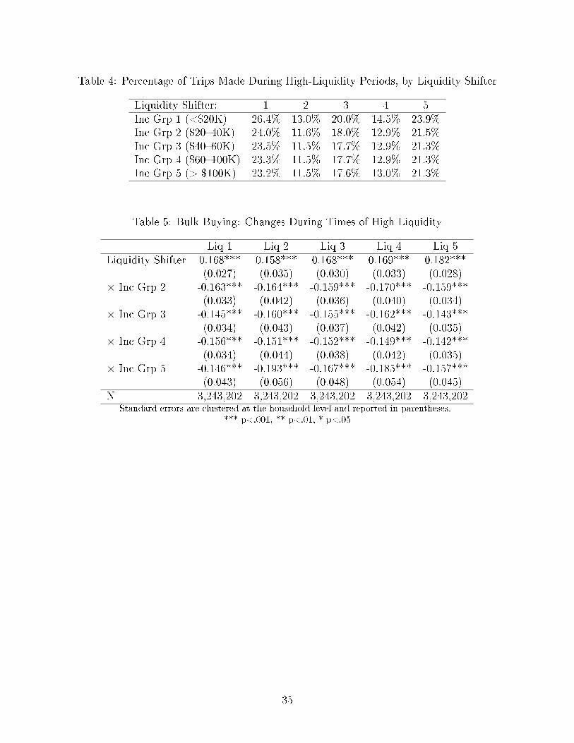
Table 4: Percentage of Trips Made During High-Liquidity Periods, by Liquidity Shifter

Liquidity Shifter: 1 2 3 4 5Inc Grp 1 (<$20K) 26.4% 13.0% 20.0% 14.5% 23.9%Inc Grp 2 ($20�40K) 24.0% 11.6% 18.0% 12.9% 21.5%Inc Grp 3 ($40�60K) 23.5% 11.5% 17.7% 12.9% 21.3%Inc Grp 4 ($60�100K) 23.3% 11.5% 17.7% 12.9% 21.3%Inc Grp 5 (> $100K) 23.2% 11.5% 17.6% 13.0% 21.3%

Table 5: Bulk Buying: Changes During Times of High Liquidity

Liq 1 Liq 2 Liq 3 Liq 4 Liq 5Liquidity Shifter 0.168*** 0.158*** 0.168*** 0.169*** 0.182***

(0.027) (0.035) (0.030) (0.033) (0.028)× Inc Grp 2 -0.163*** -0.164*** -0.159*** -0.170*** -0.159***

(0.033) (0.042) (0.036) (0.040) (0.034)× Inc Grp 3 -0.145*** -0.160*** -0.155*** -0.162*** -0.143***

(0.034) (0.043) (0.037) (0.042) (0.035)× Inc Grp 4 -0.156*** -0.151*** -0.152*** -0.149*** -0.142***

(0.034) (0.044) (0.038) (0.042) (0.035)× Inc Grp 5 -0.146*** -0.193*** -0.167*** -0.185*** -0.157***

(0.043) (0.056) (0.048) (0.054) (0.045)N 3,243,202 3,243,202 3,243,202 3,243,202 3,243,202

Standard errors are clustered at the household level and reported in parentheses.*** p<.001, ** p<.01, * p<.05

35

Table 6: Purchase Acceleration: Changes During Times of High Liquidity

Liq 1 Liq 2 Liq 3 Liq 4 Liq 5Sale -0.718** -0.836*** -0.764*** -0.830*** -0.768***

(0.228) (0.216) (0.221) (0.216) (0.222)× Inc Grp 2 -0.530* -0.375 -0.474 -0.371 -0.478***

(0.257) (0.243) (0.249) (0.244) (0.251)× Inc Grp 3 -1.051*** -1.038*** -1.086*** -1.054*** -1.122***

(0.263) (0.251) (0.256) (0.251) (0.258)× Inc Grp 4 -1.585*** -1.487*** -1.561*** -1.498*** -1.581***

(0.265) (0.252) (0.258) (0.252) (0.259)× Inc Grp 5 -1.790*** -1.734*** -1.819*** -1.725*** -1.862***

(0.322) (0.307) (0.313) (0.308) (0.315)Sale × Liquidity Shifter -1.076*** -1.319** -1.223*** -1.234** -1.007**

(0.319) (0.435) (0.358) (0.420) (0.342)× Inc Grp 2 1.197** 1.266* 1.334** 1.134* 1.153**

(0.381) (0.527) (0.431) (0.508) (0.410)× Inc Grp 3 0.681 1.485** 1.166** 1.490** 1.174**

(0.384) (0.529) (0.434) (0.513) (0.414)× Inc Grp 4 0.996** 1.386** 1.251** 1.358** 1.168**

(0.378) (0.517) (0.426) (0.499) (0.406)× Inc Grp 5 1.088* 1.924** 1.687** 1.671** 1.647***

(0.465) (0.632) (0.525) (0.611) (0.497)N 3,092,089 3,092,089 3,092,089 3,092,089 3,092,089

Standard errors are clustered at the household level and reported in parentheses.*** p<.001, ** p<.01, * p<.05

36

Table 7: Change in Bulk Buying, using Channel and Brand Controls

Using Brand+Channel ControlsLiq 1 Liq 2 Liq 3 Liq 4 Liq 5

Liquidity Shifter 0.190*** 0.144*** 0.170*** 0.153*** 0.173***(0.025) (0.031) (0.027) (0.030) (0.025)

× Inc Grp 2 -0.147*** -0.121** -0.127*** -0.130*** -0.119***(0.029) (0.037) (0.032) (0.036) (0.030)

× Inc Grp 3 -0.124*** -0.109** -0.119*** -0.115** -0.107***(0.030) (0.038) (0.032) (0.037) (0.030)

× Inc Grp 4 -0.125*** -0.106** -0.114*** -0.111** -0.104***(0.030) (0.038) (0.033) (0.037) (0.031)

× Inc Grp 5 -0.082* -0.071 -0.067 -0.065 -0.058(0.036) (0.047) (0.040) (0.045) (0.037)

Using Brand+Channel + Brand×Channel ControlsLiq 1 Liq 2 Liq 3 Liq 4 Liq 5

Liquidity Shifter 0.182*** 0.148*** 0.167*** 0.154*** 0.170***(0.024) (0.030) (0.026) (0.029) (0.024)

× Inc Grp 2 -0.154*** -0.137*** -0.141*** -0.145*** -0.134***(0.028) (0.036) (0.031) (0.035) (0.029)

× Inc Grp 3 -0.130*** -0.118** -0.130*** -0.121*** -0.119***(0.029) (0.037) (0.032) (0.036) (0.030)

× Inc Grp 4 -0.136*** -0.120** -0.126*** -0.123*** -0.115***(0.029) (0.037) (0.032) (0.036) (0.030)

× Inc Grp 5 -0.110** -0.107* -0.098* -0.097* -0.083*(0.035) (0.046) (0.038) (0.044) (0.036)

N 3,243,202 3,243,202 3,243,202 3,243,202 3,243,202Standard errors are clustered at the household level and reported in parentheses.

*** p<.001, ** p<.01, * p<.05

37

Table 8: Change in Purchase Acceleration, using Channel and Brand Controls

Using Brand+Channel ControlsLiq 1 Liq 2 Liq 3 Liq 4 Liq 5

Liquidity×Sale -1.085*** -1.324** -1.235*** -1.250** -1.026**(0.318) (0.434) (0.358) (0.420) (0.342)

× Inc Grp 2 1.217** 1.243* 1.340** 1.119* 1.162**(0.381) (0.526) (0.430) (0.508) (0.409)

× Inc Grp 3 0.686 1.440** 1.151** 1.450** 1.150**(0.383) (0.528) (0.434) (0.512) (0.413)

× Inc Grp 4 0.998** 1.299* 1.210** 1.288** 1.134**(0.378) (0.516) (0.426) (0.498) (0.406)

× Inc Grp 5 1.122* 1.912** 1.688** 1.672** 1.660***(0.464) (0.631) (0.524) (0.610) (0.496)

Using Brand+Channel + Brand×Channel ControlsLiq 1 Liq 2 Liq 3 Liq 4 Liq 5

Liquidity×Sale -1.101*** -1.343** -1.251*** -1.263** -1.037**(0.318) (0.434) (0.358) (0.420) (0.342)

× Inc Grp 2 1.216** 1.259* 1.350** 1.133* 1.170**(0.381) (0.526) (0.430) (0.507) (0.409)

× Inc Grp 3 0.686 1.446** 1.158** 1.455** 1.156**(0.383) (0.528) (0.434) (0.512) (0.413)

× Inc Grp 4 1.008** 1.314** 1.221** 1.298** 1.139**(0.378) (0.516) (0.426) (0.498) (0.406)

× Inc Grp 5 1.111* 1.894** 1.677** 1.648** 1.639**(0.464) (0.631) (0.523) (0.610) (0.496)

N 3,092,089 3,092,089 3,092,089 3,092,089 3,092,089Standard errors are clustered at the household level and reported in parentheses.

*** p<.001, ** p<.01, * p<.05

38

Table 9: Change in Bulk Buying, controlling for supply-side variation

Using Sale Frequency ControlsLiq 1 Liq 2 Liq 3 Liq 4 Liq 5

Liquidity Shifter -0.141*** -0.100** -0.119*** 0.033 0.022(0.028) (0.035) (0.030) (0.034) (0.028)

× Inc Grp 2 -0.134*** -0.144*** -0.130*** -0.158*** -0.135***(0.033) (0.042) (0.036) (0.041) (0.034)

× Inc Grp 3 -0.121*** -0.147*** -0.131*** -0.158*** -0.128***(0.035) (0.044) (0.037) (0.042) (0.035)

× Inc Grp 4 -0.104** -0.122** -0.109** -0.135** -0.119***(0.035) (0.044) (0.038) (0.042) (0.035)

× Inc Grp 5 -0.084* -0.146** -0.109* -0.159** -0.125**(0.043) (0.055) (0.047) (0.053) (0.044)

Using Brand×Liquidity and Channel×Liquidity ControlsLiq 1 Liq 2 Liq 3 Liq 4 Liq 5

Liquidity Shifter 0.148*** 0.069* 0.096** 0.056 0.062*(0.033) (0.032) (0.029) (0.031) (0.027)

× Inc Grp 2 -0.145*** -0.122** -0.126*** -0.130*** -0.116***(0.029) (0.037) (0.032) (0.036) (0.030)

× Inc Grp 3 -0.122*** -0.110** -0.118*** -0.115** -0.105***(0.030) (0.038) (0.033) (0.037) (0.031)

× Inc Grp 4 -0.123*** -0.108** -0.114*** -0.110** -0.100**(0.030) (0.039) (0.033) (0.037) (0.031)

× Inc Grp 5 -0.082* -0.075 -0.070 -0.067 -0.058(0.037) (0.048) (0.040) (0.046) (0.038)

Using Brand×Channel×Liquidity Shifter ControlsLiq 1 Liq 2 Liq 3 Liq 4 Liq 5

Liquidity Shifter 0.235*** 0.089*** 0.116*** 0.075** 0.084**(0.039) (0.031) (0.029) (0.030) (0.026)

× Inc Grp 2 -0.149*** -0.134** -0.136*** -0.141*** -0.128***(0.028) (0.036) (0.031) (0.035) (0.029)

× Inc Grp 3 -0.123*** -0.113** -0.123*** -0.115** -0.110***(0.029) (0.037) (0.032) (0.036) (0.030)

× Inc Grp 4 -0.125*** -0.112** -0.117*** -0.113** -0.101***(0.029) (0.037) (0.032) (0.036) (0.030)

× Inc Grp 5 -0.094** -0.097* -0.087* -0.085 -0.068(0.036) (0.046) (0.039) (0.044) (0.037)

N 3,243,202 3,243,202 3,243,202 3,243,202 3,243,202Standard errors are clustered at the household level and reported in parentheses.

*** p<.001, ** p<.01, * p<.05

39

Table 10: Change in Purchase Acceleration, controlling for supply-side variation

Using Sale Frequency ControlsLiq 1 Liq 2 Liq 3 Liq 4 Liq 5

Liquidity×Sale -1.044** -1.308** -1.210*** -1.252** -1.019**0.318 0.434 0.358 0.421 0.342

× Inc Grp 2 1.207** 1.262* 1.346** 1.136* 1.165**0.381 0.526 0.431 0.508 0.410

× Inc Grp 3 0.680 1.479** 1.162** 1.485** 1.167**0.383 0.529 0.434 0.513 0.414

× Inc Grp 4 0.992** 1.375** 1.249** 1.353** 1.161**0.378 0.517 0.426 0.499 0.406

× Inc Grp 5 1.106* 1.947** 1.703** 1.692** 1.666***0.464 0.631 0.524 0.611 0.497

Using Brand×Liquidity and Channel×Liquidity ControlsLiq 1 Liq 2 Liq 3 Liq 4 Liq 5

Liquidity×Sale -1.083*** -1.239** -1.125** -1.201** -0.938**0.322 0.436 0.361 0.421 0.344

× Inc Grp 2 1.224** 1.265* 1.370** 1.138* 1.190**0.381 0.526 0.430 0.508 0.409

× Inc Grp 3 0.699 1.464** 1.179** 1.474** 1.179**0.383 0.528 0.434 0.512 0.413

× Inc Grp 4 1.018** 1.322* 1.236** 1.311** 1.159**0.378 0.516 0.426 0.499 0.406

× Inc Grp 5 1.149** 1.914** 1.684** 1.676** 1.652***0.464 0.631 0.524 0.610 0.497

Using Brand×Channel×Liquidity Shifter ControlsLiq 1 Liq 2 Liq 3 Liq 4 Liq 5

Liquidity×Sale -1.102*** -1.280** -1.167** -1.238** -0.985**(0.322) (0.436) (0.361) (0.421) (0.344)

× Inc Grp 2 1.223** 1.266* 1.367** 1.141* 1.188**(0.381) (0.526) (0.430) (0.507) (0.409)

× Inc Grp 3 0.686 1.449** 1.165** 1.462** 1.166**(0.383) (0.528) (0.434) (0.512) (0.413)

× Inc Grp 4 1.011** 1.314* 1.228** 1.309** 1.153**(0.378) (0.516) (0.426) (0.498) (0.406)

× Inc Grp 5 1.113* 1.872** 1.649** 1.636** 1.616**(0.465) (0.631) (0.524) (0.610) (0.497)

N 3,092,089 3,092,089 3,092,089 3,092,089 3,092,089Standard errors are clustered at the household level and reported in parentheses.

*** p<.001, ** p<.01, * p<.05

40

Table 11: Placebo Tests: Changes During Times of High Liquidity

Coupon Use Store Brand Cheap BrandLiquidity Shifter (�rst 7 days) -0.0006 -0.0050*** 0.0020

(0.0012) (0.0015) (0.0014)× Inc Grp 2 -0.0009 0.0026 -0.0007

(0.0014) (0.0017) (0.0016)× Inc Grp 3 -0.0014 0.0045** -0.0004

(0.0015) (0.0017) (0.0016)× Inc Grp 4 -0.0011 0.0046** -0.0011

(0.0015) (0.0017) (0.0016)× Inc Grp 5 -0.0032 0.0045* -0.0018

(0.0018) (0.0019) (0.0018)N 3,250,995 3,250,995 3,250,995

Standard errors are clustered at the household level and reported in parentheses.*** p<.001, ** p<.01, * p<.05

Figure 1: Percentage Deviation of Average Daily Store Visit and Spending Patterns fromMonthly Average, by Income Group

41

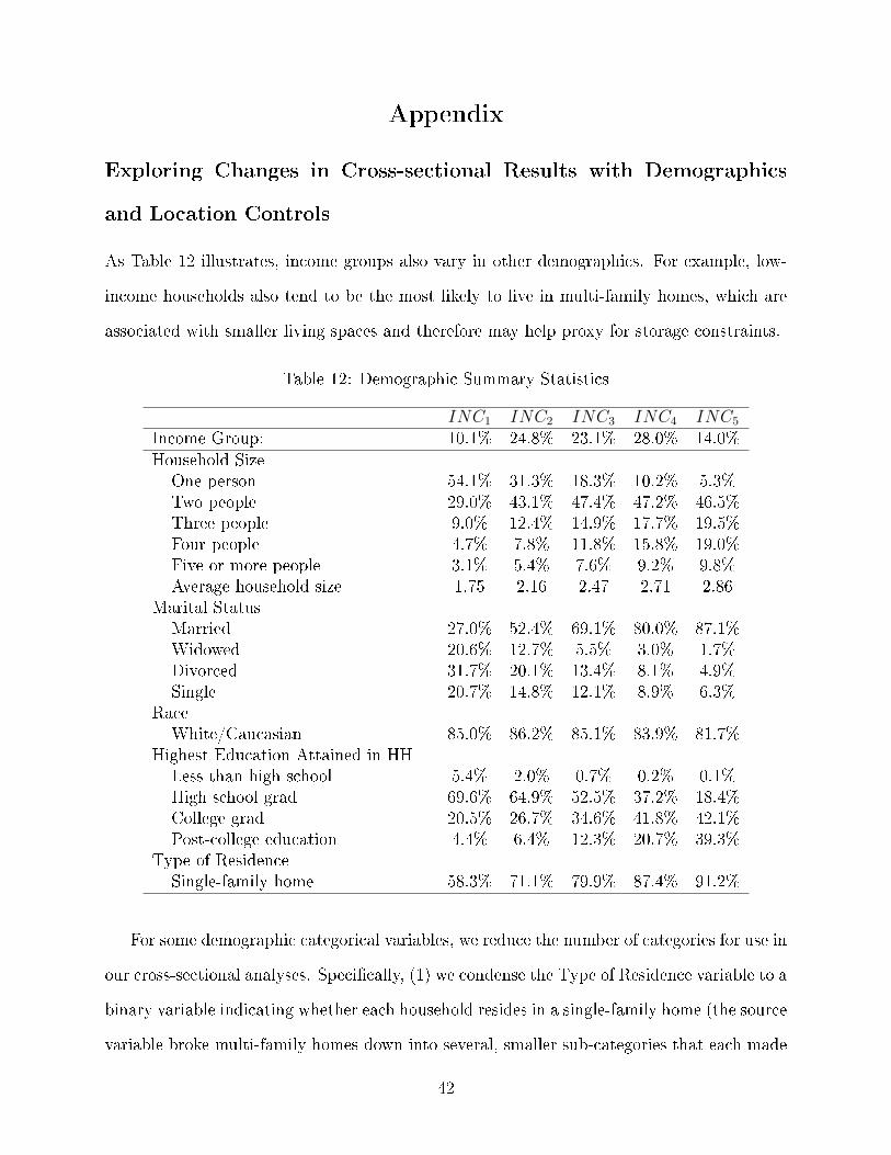
Appendix

Exploring Changes in Cross-sectional Results with Demographics

and Location Controls

As Table 12 illustrates, income groups also vary in other demographics. For example, low-

income households also tend to be the most likely to live in multi-family homes, which are

associated with smaller living spaces and therefore may help proxy for storage constraints.

Table 12: Demographic Summary Statistics

INC1 INC2 INC3 INC4 INC5

Income Group: 10.1% 24.8% 23.1% 28.0% 14.0%Household Size

One person 54.1% 31.3% 18.3% 10.2% 5.3%Two people 29.0% 43.1% 47.4% 47.2% 46.5%Three people 9.0% 12.4% 14.9% 17.7% 19.5%Four people 4.7% 7.8% 11.8% 15.8% 19.0%Five or more people 3.1% 5.4% 7.6% 9.2% 9.8%Average household size 1.75 2.16 2.47 2.71 2.86

Marital StatusMarried 27.0% 52.4% 69.1% 80.0% 87.1%Widowed 20.6% 12.7% 5.5% 3.0% 1.7%Divorced 31.7% 20.1% 13.4% 8.1% 4.9%Single 20.7% 14.8% 12.1% 8.9% 6.3%

RaceWhite/Caucasian 85.0% 86.2% 85.1% 83.9% 81.7%

Highest Education Attained in HHLess than high school 5.4% 2.0% 0.7% 0.2% 0.1%High school grad 69.6% 64.9% 52.5% 37.2% 18.4%College grad 20.5% 26.7% 34.6% 41.8% 42.1%Post-college education 4.4% 6.4% 12.3% 20.7% 39.3%

Type of ResidenceSingle-family home 58.3% 71.1% 79.9% 87.4% 91.2%

For some demographic categorical variables, we reduce the number of categories for use in

our cross-sectional analyses. Speci�cally, (1) we condense the Type of Residence variable to a

binary variable indicating whether each household resides in a single-family home (the source

variable broke multi-family homes down into several, smaller sub-categories that each made

42

Table 13: Cross-Sectional Di�erences in Di�erent Saving Strategies: Additional ControlsBuy Store Brand Buy Cheapest Brand Package Size

(1) (2) (3) (1) (2) (3) (1) (2) (3)

Income Grp 2-0.04*** -0.04*** -0.04*** -0.02*** -0.02*** -0.01*** 0.9*** 0.7*** 0.5***

(0.006) (0.006) (0.004) (0.003) (0.003) (0.002) (0.10) (0.11) (0.08)

Income Grp 3-0.07*** -0.06*** -0.06*** -0.03*** -0.04*** -0.02*** 1.6*** 1.2*** 0.9***

(0.006) (0.006) (0.005) (0.003) (0.003) (0.002) (0.11) (0.12) (0.09)

Income Grp 4-0.09*** -0.08*** -0.09*** -0.03*** -0.05*** -0.02*** 2.9*** 2.2*** 1.7***

(0.006) (0.006) (0.005) (0.003) (0.003) (0.002) (0.11) (0.13) (0.10)

Income Grp 5-0.10*** -0.10*** -0.10*** -0.03*** -0.05*** -0.01*** 4.7*** 3.5*** 2.7***

(0.006) (0.007) (0.005) (0.003) (0.004) (0.003) (0.13) (0.15) (0.13)

Controls

Consumption Yes Yes Yes Yes Yes Yes Yes Yes Yes

Demographic No Yes Yes No Yes Yes No Yes Yes

Location No No Yes No No Yes No No Yes

N 2,898,666 2,898,666 2,891,525

Note: We report results from 4-digit zipcodes that include at least 10 reporting panelists.Standard errors are clustered at the household level and reported in parentheses.

*** p<.001, ** p<.01, * p<.05

up a small percentage of observations in the Nielsen data set), (2) for the male and female

head of a household's education (two separate variables), we divide households by whether

they graduated from high school and graduated from college (rather than distinguishing, for

example, between a high school graduate with no college and one with a little bit of college),

(3) we condense the Race variable into a binary variable indicating whether the household

head is caucasion or not, since the vast majority of household heads were caucasian, and (4)

combine all households of size greater than or equal to �ve into a single category, since there

were very few households with more than �ve occupants.

Table 13 introduces additional controls to the cross-sectional results presented in Table

2. For each dependent variable, column 1 repeats the main cross-sectional speci�cation that

has consumption rate controls. Column 2 includes levels of all demographics summarized in

Table 12 as indicator variables. Column 3 adds �xed e�ects for each 4-digit zipcode with

more than 10 reporting households. All speci�cations are run on a subsample that includes

only observations from panelists living in 4-digit zipcodes with a minimum of 10 reporting

households for ease of comparison across three speci�cations. We see that the degree of cross-

43

Table 14: Di�erence in Duration after Purchase for Sale and Non-sale Purchases

Variable I[sale] Inc 2 * I[sale] Inc 3 * I[sale] Inc 4 * I[sale] Inc 5 * I[sale]Coe�cient δ1 δ2 δ3 δ4 δ5

Inter-purchase time4.753*** -0.860*** -1.680*** -2.561*** -2.680***(0.236) (0.257) (0.267) (0.269) (0.321)

Number of Obs. 3,133,108Standard errors are clustered at the household level and reported in parentheses.

*** p<.001, ** p<.01, * p<.05

sectional di�erences across income groups in buying store brands does not change with added

controls. On the other hand, the di�erences in the propensity to purchase the cheapest brand

respond signi�cantly to the addition of location controls. The extent to which households

di�er in their bulk-buying habits also responds to the addition of demographics and location

controls, although large cross-sectional di�erences in this behavior remain even after we

control for these factors.

Duration After Purchase

To check whether the di�erence in interpurchase timing across households is due, at least in

part, to purchase acceleration, rather than an increase in consumption, we test whether the

time until the next purchase occasion (Durationhtp) increases in response to purchasing on

sale using the following speci�cation:

Durationhtp = αh + δhI[sale]htp +∑5

i=2 νiI[INCht = i] +∑3

j=1 µj[Consumption]jh + εhtp

where δh = δ1 +∑5

i=2 δiI[INCht = i] +∑3

j=1 µj[Consumption]jh.

Consistent with stockpiling behavior, the results in Table 14 illustrate that households

waited longer before purchasing again following sale purchases than they did following non-

sale purchases (δ0 > 0). Interestingly, this di�erence is greatest for low-income households

(δi < 0 for i > 2), even though high income households display greater purchase acceleration.

44