arX

iv:h

ep-t

h/04

0720

7v1

23

Jul 2

004

From the Dirac Operator to Wess-Zumino

Models on Spatial Lattices

A. Kirchberg, J.D. Lange and A. Wipf∗

Theoretisch–Physikalisches Institut,

Friedrich–Schiller–Universitat Jena,

07743 Jena, Germany

FSU-TPI 04/04

Abstract: We investigate two-dimensional Wess-Zumino models in the continuum andon spatial lattices in detail. We show that a non-antisymmetric lattice derivative notonly excludes chiral fermions but in addition introduces supersymmetry breaking latticeartifacts. We study the nonlocal and antisymmetric SLAC derivative which allows forchiral fermions without doublers and minimizes those artifacts. The supercharges of thelattice Wess-Zumino models are obtained by dimensional reduction of Dirac operatorsin high-dimensional spaces. The normalizable zero modes of the models with N = 1 andN = 2 supersymmetry are counted and constructed in the weak- and strong-couplinglimits. Together with known methods from operator theory this gives us complete controlof the zero mode sector of these theories for arbitrary coupling.

Keywords: Lattice, Supersymmetry, Dirac Operator

PACS: 11.10.Kk, 11.30.Pb, 12.60.Jv

∗A.Kirchberg@tpi.uni-jena.de, J.D.Laenge@tpi.uni-jena.de, A.Wipf@tpi.uni-jena.de

1

1 Introduction

Ever since its invention supersymmetry has been an important subject in high-energyphysics beyond the standard model. It is considered to be a necessary ingredient tobridge the gap between the scale of electroweak symmetry breaking and the much largerunification scale. Nowadays, supersymmetric theories cover the whole range from su-persymmetric classical mechanics [1], quantum mechanics [2, 3], scalar and gauge fieldtheories [4] to string- and M -theory [5]. They allow for the construction of low-energyeffective actions, as for the N = 2 Seiberg-Witten model [6] or the formulation of certainduality relations, like in the original Maldacena conjecture for gauge theories with N = 4extended supersymmetry [7].

The non-perturbative effects in supersymmetric theories, and in particular, the dynam-ical breaking of supersymmetry are a subject of intensive studies. At present time thelattice formulation is the only tool for systematic investigations of such effects, and lat-tice simulations provide the means of doing reliable calculations in the strong-couplingregime or near a phase transition point. After the pioneering work of Dondi and Nico-lai [8] there has been an ongoing effort into formulating, understanding and simulatingsupersymmetric theories on the lattice [9, 10, 11, 12]. Recent lattice results, e.g. on thebreaking of supersymmetry, have been obtained in [13, 14, 15].

A commonly accepted guiding principle in any good lattice calculation is to build in asmany of the symmetries of the continuum model as possible, such that the lattice resultsrespect these symmetries identically. However, often these are conflicting requirementsand not all symmetries can be incorporated on the lattice. This in turn introduces subtlelattice artifacts into the formalism, which one may not get rid of in the continuum limit.For example, lattice regularizations of supersymmetric theories generically break large

parts of supersymmetry, and it is a nontrivial problem to recover supersymmetry inthe continuum limit. However, there are discretizations with highly nonlocal derivativeoperators, for which supersymmetry is manifestly realized [8, 11]. Alternatively, for two-dimensional models one can discretize only space (time remains continuous) such that asubalgebra of the N = 1 supersymmetry algebra,

Qα, Qβ = 2(γµγ0)αβPµ

remains intact [9, 10, 16]. That subalgebra then determines the spectral properties ofthe super-Hamiltonian H. The fermion doubling for naive lattice derivatives [17, 18]is another apparently unrelated notorious example of such lattice artifacts. For bosonsthere is no such problem. However, if we try to preserve part of supersymmetry thenthe fermionic mirror states lead to doublers in the bosonic sector as well.

In this paper we study continuum and lattice versions of two-dimensional Wess-Zumino(WZ) models. Similar to the original four-dimensional theory [19], these models containscalar and fermion fields coupled by a Yukawa term. A particular version possessesN = 2 supersymmetry and has been the subject of analytic [20, 21] and numerical [22]studies.

2

In section 2 we consider the off-shell formulation for a general class of continuum mod-els and derive the supersymmetry transformations and Noether currents. Particularemphasis is put on the form of the central charges [23].

In section 3 we turn to the lattice version of the models. We show that for real andantisymmetric lattice derivatives the N = 1 algebra can be represented on free fields.The local left- and right-derivatives are not antisymmetric and the anticommutator ofthe corresponding supercharges does not yield the discretized Hamiltonian for the freemodel. If we insist that supersymmetry is realised on free fields without fermion andboson doubling then we must allow for nonlocal derivatives on the lattice. One particularsuch derivative, the SLAC operator, is introduced in this section. The numerical resultsfor this operator concerning supersymmetry in lower-dimensional systems are in excellentagreement with continuum results. In section 4 we show how to derive the models withN = 1 andN = 2 supersymmetry on a spatial lattice by a suitable dimensional reduction

of a high-dimensional Euclidean Dirac operator. In the process of reduction the Diracmatrices and coordinates turn into Majorana spinors and scalar fields on the lattice.We count and construct the normalisable eigenstates of H with zero energy both in theweak and strong-coupling limits. In particular we find that the N = 2 models with φ2q

interaction admit qN such states if N is the number of spatial lattice sites.

In section 4 we bridge the gap between strong- and weak-coupling regimes for modelswith N = 1 and N = 2 supersymmetry with the help of powerful methods from operatortheory. Using a theorem by Kato we prove that the zero modes in the strong-couplinglimit survive for intermediate couplings as long as the coupling constant of the leadingterm in the potential does not vanish. We comment on what we expect to happen in thecontinuum limit of theN = 2 models, where only q of the qN zero modes survive [24]. Wealso comment on recent lattice simulations of the two dimensional Wess-Zumino modelby Beccaria et al. [25]. Some technical details concerning the nonlocal SLAC operatorand the proof that the transition from strong to intermediate couplings is governed bya relative compact perturbation are relegated to the appendix.

2 Wess-Zumino Models in 1 + 1 Dimensions

In the off-shell formulation two-dimensional parity invariant Wess-Zumino models con-tain a set of, say d, triples, each containing a real scalar φ, Majorana spinor ψ andauxiliary field F . In a Majorana representation for the Clifford algebra

γµ, γν = 2ηµν , with γ0㵆γ0 = γµ, η = diag(1,−1), (1)

the Majorana spinors are real.

The supersymmetry algebra is spanned by N Hermitian spinorial supercharges Q(I),I = 1, . . . ,N , by the Hermitian two-momentum Pµ and by the (anti-)symmetric matrix

3

of Hermitian central charges ZIJS (ZIJA ) and has the form

Q(I)α , Q

(J)β = 2

(δIJ /Pαβ + iδαβZIJ

A + iγ∗αβZIJS

), γ∗ = γ0γ1, (2)

with spinor index α = 1, 2.

In component fields the Lagrangian of the models with N = 1 supersymmetry reads [26]

L = 12∂µφ

a∂µφa − F aW,a+12F

aFa +i2 ψ

a/∂ψa − 12W,ab ψ

aψb, (3)

where the superpotential W depends on the dimensionless scalar fields φ1, . . . , φd. Wedenoted the derivative of W with respect to φa by W,a and employed the Einstein sum-mation convention. For Wess-Zumino models the target spaces are Rd with Euclideanmetric δab.

Now we consider the most general linear off-shell supersymmetry transformation of thefields. Since (φa, ψa, F a) have mass dimensions (0, 12 , 1) respectively, such transforma-tions have the form [26]

δǫφa = ǫ(Aψ)a,

δǫψa = i/∂ (Bφ)aǫ+ (CF )aǫ, (4)

δǫFa = iǫ/∂ (Dψ)a,

where, for example, (Aψ)a = Aabψb. The constant matrices A,B,C,D must be real for

the supersymmetry variations to be Hermitian fields. The requirement that L transformsinto a divergence implies the following algebraic relations for these matrices and the realsymmetric matrix W ′′ = (W,ab ),

A+BT = 0, D + CT = 0, (5)

ATW ′′ +W ′′C = 0, W ′′AT + CW ′′ = 0. (6)

It follows that

δL = ǫ ∂µVµ +∆ with ∆ = −1

2W,abc(ǫAadψ

d) (ψbψc

).

Free models have quadratic superpotentials and ∆ is identically zero. For interactingmodels we may exploit the Fierz identity

(ψaψb)(ψcψd) + (ψaψd)(ψbψc) + (ψaψc)(ψdψb) = 0

to prove that ∆ vanishes, provided

W ′′A = ATW ′′ (7)

holds true. Then the action is left invariant by the transformations (4) and the corre-sponding conserved Noether current reads

Jµ = (∂µφ− γ∗ǫµν∂νφ)

a (Aψ)a − i(CW ′)aγµψa, W ′ = (∂W/∂φa) . (8)

4

In what follows, employing (5), we express the matrices B and D in terms of A and C.We considerN supersymmetries (4) with matrices (AI , CI) and denote the corresponding

supersymmetry transformations by δ(I)ǫ . For all pairs (AI , CI) the conditions (6) and

(7) must hold for the Lagrangian to be invariant. These conditions severely restrict theform of the superpotentialW . We also demand that two supersymmetry transformationsclose on translations (later we shall comment on the possibility of central charges)

[δ(I)ǫ1 , δ

(J)ǫ2

]Φ = 2iδIJ(ǫ2γ

µǫ1)∂µΦ, (9)

and this puts further restrictions on the matrices. For the scalar and the auxiliary fieldthe condition (9) read

AIATJ +AJA

TI = CTI CJ + CTJ CI = 2δIJ1 and AICJ −AJCI = 0. (10)

In particular all matrices are orthogonal, such that the two conditions in (6) coincide.Actually, the last relation implies that the algebra (9) is realized on the Majorana fieldsas well.

The transformation δ(I)ǫ is generated by the Noether charge corresponding to JµI in (8),

Q(I) =

∫

dx((π − φ′γ∗)a(AIψ)

a − i(CIW′)aγ

0ψa), πa = φa, (11)

where we have set (dφa/dx) = φ′.

Canonical structure: The canonical structure is more transparent in the on-shell for-mulation. This is obtained from the off-shell one by replacing Fa by W,a. The nontrivialequal time (anti)commutators between the scalar fields, their conjugated momentumfields πa = φa and the Majorana fields read

ψaα(x), ψbβ(y) = δαβδabδ(x− y) and [φa(x), πb(y)] = iδabδ(x − y). (12)

The Hamiltonian is the Legendre transform of the Lagrangian,

H =

∫

dxH, H = 12π · π + 1

2φ′ · φ′ + 1

2W′ ·W ′ + 1

2ψ†hFψ, (13)

where, for example, π ·π = πaπa. We have introduced the Hermitian Dirac-Hamiltonian

(hF)ab = −iγ∗∂xδab + γ0W,ab≡ (h0F)ab + γ0W,ab . (14)

The action is invariant under spacetime translations generated by Noether charges

P0 = H and P1 =

∫

dx(π · φ′ + i

2 ψγ0ψ′), (15)

and under supersymmetry transformations (4) generated by the above superchargesQ(I).By using the relations (6,10) one proves that the Q(I) satisfy the super-algebra (2) withcentral charges

ZIJA = 0 and ZIJ

S = −∫

φ′ ·(AICJ

)W ′, (16)

5

where we have neglected ambiguous surface terms containing the Majorana fields only.Note, that the integrand is a total derivative, since the integrability conditions for theexistence of a potential U(φ(x)) with

φ′ · (AICJ)W ′ =dU

dx= U ′ · φ′

is that AICJW′′ is a symmetric matrix. But this follows from the condition (6).

In most explicit calculations we choose the Majorana representation

γ0 = σ2, γ1 = iσ3 and γ∗ = γ0γ1 = −σ1 (17)

such that the superalgebra takes the simple form

Q(I)1 , Q

(J)1 = 2

(HδIJ +ZIJ

S

),

Q(I)2 , Q

(J)2 = 2

(HδIJ −ZIJ

S

), (18)

Q(I)1 , Q

(J)2 = 2

(P1δ

IJ + ZIJA

).

N = 1 supersymmetry: There is always at least one solution to the constraints (5,6,7)and (10) for an arbitrary superpotential W , namely

A1 = −B1 = −C1 = D1 = 1. (19)

Solving for the auxiliary field, Fa =W,a, the on-shell transformations take the form

δ(1)ǫ φ = ǫψ, δ(1)ǫ ψ =(−i/∂φ−W ′

)ǫ, (20)

and the corresponding supercharge reads

Q(1) =

∫

dx(π − φ′γ∗ + iW ′γ0

)· ψ . (21)

For vanishing spinors the only non-trivial central charge is

ZS =

∫

dxdW

dx. (22)

N = 2 extended supersymmetry: We assume that the model (3) admits a secondsupersymmetry besides the solution (19). The conditions (10) imply

A2 = −C2 = I, I = −IT , I2 = −1. (23)

The matrix I defines a complex structure and exists for all target spaces Rd with evendimension d. The conditions in (6) and (7) on the superpotential both reduce to

IW ′′ +W ′′I = 0, (24)

6

which means that the superpotential is a harmonic function of the scalar fields, in agree-ment with the general analysis in [26]. On-shell, the second supersymmetry has theform

δ(2)ǫ φ = ǫIψ, δ(2)ǫ ψ =(i/∂ Iφ− IW ′

)ǫ, (25)

and is generated by the Noether-supercharge

Q(2) =

∫

dx(π − φ′γ∗ − iW ′γ0

)· (Iψ). (26)

For vanishing spinor fields the central charges read

ZIJA = 0 and

(ZIJS

)= σ3

∫

dxdW

dx− σ1

∫

dxdU

dx, (27)

where U is the imaginary part of the analytic function F (φ1+iφ2) = W + iU with realpart W .

For the models with N = 2 supersymmetry there exists a concise formulation in whichtwo real scalars are combined to a complex scalar, and two Majorana spinors are com-bined to a Dirac spinor. For example, for the target space R2 we set

φ =1√2

(φ1 + iφ2

), ψ =

1√2

(ψ1 + iγ∗ψ

2). (28)

The harmonic superpotential is the real part of a holomorphic function,

W (φ, φ) = F (φ) + F (φ), (29)

and the on-shell Lagrangian takes the form

L = ∂µφ∂µφ† + iψ /∂ψ − 1

2 |F ′|2 − F ′′ψP+ψ − F ′′ψP−ψ, (30)

where F ′ is the derivative of F with respect to the complex field φ and we have introducedthe chiral projectors

P± = 12(1+ γ∗). (31)

Along with the real scalar fields one combines the corresponding conjugate momentumfields to a complex momentum, π = (π1−iπ2)/

√2, such that

[φ(x), π(y)] = iδ(x − y) and ψα, ψ†β = δαβ . (32)

The complex supercharge takes the form

Q = 12

(

Q(1) + iγ∗Q(2))

=(π − φ′ + iF ′γ0

)P+ψ +

(π + φ′ + iF ′γ0

)P−ψ. (33)

and satisfies the anticommutation relations

Q,Q = 0 and Q, Q = /P + γ∗Z11S −Z12

S . (34)

7

Higher supersymmetries: Next we show that with the absence of central chargesthere is no third linear off-shell supersymmetry besides (20) and (25). To be compat-ible with the first transformation in (20), the orthogonal matrices A3 and C3 must beantisymmetric and of opposite sign. The conditions (10) between the second and thirdsupersymmetry imply

[I,A3] = I,A3 = 0,

which is impossible for orthogonal matrices I and A3. We conclude that the models (3)admit at most two linear off-shell supersymmetries.

Let us mention that, if we allow for central charges in the superalgebra, there existfurther supersymmetries. But the corresponding models are massive free models. Theycan be derived by a dimensional reduction of the free N = 2 model in 4 dimensions.

3 Lattice Formulations of Wess-Zumino Models

As ultraviolet-cutoff we discretize space, introduce a spatial lattice with N equidistantsites and choose periodic boundary conditions. The time is kept continuous such thattime translations remain symmetries generated by the Hamiltonian. Following [9] we tryto preserve at least that subalgebra of (2) which involves H.

The fields of the supersymmetric model in the Hamiltonian formulation are discretizedas follows,

(φa(x), πa(x), ψa(x)) −→ (φa(n), πa(n), ψa(n)) , n = 1, . . . , N, (35)

where the lattice spacing has been set to one. On a space-lattice the derivative becomesa difference operator the particular choice of which is left open for the moment being.We define the lattice Hamiltonian as square of the discretized supercharge Q1. Forinteracting theories it consists of the discretized Hamiltonian of the continuum theoryplus a lattice counterpart of the central charge.

On-shell the N = 1 model contains d ∈ 1, 2, . . . Hermitian scalar fields φa(n) and dMajorana spinors ψa(n) on N lattice sites (n = 1, . . . , N). The fields obey the non-trivialcanonical (anti-)commutation relations

[φa(n), πb(n′)] = iδabδ(n, n′) and ψaα(n), ψbβ(n′) = δabδαβδ(n, n′). (36)

We choose a Majorana representation such that the ψa are Hermitian two componentspinors.

When we put the supercharge on a space-lattice, we must choose the lattice derivativein the term

−∫

φ′γ∗ψ =

∫

φγ∗ψ′ = i

∫

φh0Fψ

8

in (11). Since we do not want to specify ∂ at this point we make the general ansatz forthe Hermitian Dirac-Hamiltonian

h0F= iδab

(0 ∂

−∂† 0

)

, with ∂∂† = ∂†∂ ≡ − (37)

and a real ∂ with correct continuum limit. ∂ must be real, since it should map Majoranaspinors into Majorana spinors. Let us define its symmetric and antisymmetric parts

∂S = 12(∂ + ∂†), ∂A = 1

2 (∂ − ∂†) with [∂A, ∂S] = 0, ∂2A− ∂2

S= . (38)

The last two properties follow from our assumption [∂, ∂†] = 0 in (37). Since

h0F

(17)= −iγ∗∂A − γ0∂S, (39)

chirality is preserved for massless fermions if ∂ = ∂A is antisymmetric, in which caseh0

F= −iγ∗∂A. Thus, if ∂ is antisymmetric and local then, according to some long-

standing no-go theorems there is fermion doubling. There are many such theorems, andwe mention only two, one due to Nielsen and Ninomiya [17] and a later elaboration dueto Friedan [18]. No-go theorems are notorious in that people find a way around them,and following Friedans work, Luscher [27] and others did so. Below we circumvent theno-go theorems by using a nonlocal and antisymmetric derivative.

However, most lattice derivative are not antisymmetric in which case h0Fcontains a

momentum dependent mass term −γ0∂S. Such a chirality violating term has been in-troduced by Wilson [28] to raise the masses of the unwanted doublers to values of orderof the cutoff, thereby decoupling them from continuum physics.

As discretized supercharge (21) we take

Q(1) = (π, ψ) + i(φ, h0Fψ) + i(W ′, γ0ψ). (40)

A careful calculation yields the following anticommutation relations,

12Q(1)

α , Q(1)β = (/Pγ0)αβ − i(γ1)αβ(W

′, ∂Aφ)− δαβ(W′, ∂Sφ) (41)

with energy and momentum

2P0 = (π, π)− (φ,φ) +(W ′,W ′

)+ (ψ, hFψ) ,

2P1 = 2(∂Aφ, π

)−(ψ, γ∗h

0Fψ), hF = h0

F+ γ0W ′′. (42)

To arrive at these results one uses the identity

(π, ∂φ) + i(∂†ψ1, ψ1) = (∂φ, π) − i(ψ1, ∂†ψ1),

which holds for any real difference operator ∂. The superalgebra can be rewritten as

12Q(1), Q(1) = /P + iγ∗(W

′, ∂Aφ)− γ0(W ′, ∂Sφ). (43)

9

The last term is absent in the superalgebra (2) and breaks Lorentz covariance explicitly.This lattice artifact originates in the Wilson term −γ0∂S in (39). This term must vanishin the continuum limit. One may wonder whether there exist other improvement termswe could add to a local −iγ∗∂A in order to avoid the fermion doubling. However, sincefor Majorana fermions the terms

(ψ, ∂Sψ), (ψ, γ1∂Sψ), (ψ, γ∗∂Sψ)

are constant or zero, all terms but γ0∂S do not show up in the right hand side of (42)and we obtain the same result as if we had chosen hF = −iγ∗∂A. Hence only the Wilsonterm ∼ γ0∂S can be used to avoid the fermion doubling. This argument does not applyto theories with several Majorana fermions and in particular to models with extendedsupersymmetry.

Models with N = 2 supersymmetry contain the second supercharge in (26), the latticeversion of which reads

Q(2) = (π, Iψ) + i(φ, h0FIψ)− i(W ′, γ0Iψ), (44)

and satisfies the same anticommutation relations as Q(1), up to a sign change of the lasttwo terms in (43). The anticommutator of two lattice charges reads

12Q(I), Q(J) = δIJ /P + iγ∗ZIJ

S +ZIJL , (45)

where the ‘would-be’ central charges

ZIJS = σIJ3 (W ′, ∂Aφ)− (σ1)

IJ(U ′, ∂Aφ) (46)

approach the central charges (27) of the continuum model. To arrive at (45) one needsthe harmonicity of the superpotential which in turn implies the existence of a functionU(φ) with IW ′ = U ′, and this function enters the central charges. However, since theLeibniz rule never holds on the lattice, the integrands W ′ · ∂Aφ and U ′ · ∂Aφ in (46) arenot just total derivatives as in the continuum and as a consequence the terms ZIJ

S arenot central to the algebra. The annoying terms

ZIJL = −(σ3)

IJγ0(W ′, ∂Sφ) + (σ1)IJ(γ0(U ′, ∂Sφ)− i(π, I∂Sφ)− i

2(ψ, I∂Sψ))

(47)

in (45) are pure lattice artifacts and vanish for antisymmetric lattice derivatives.

Free Wess-Zumino model (N = 1): For simplicity we consider the free model withscalars of equal mass. The superpotential reads W = 1

2mφaφa and with W ′ = mφ the

‘would-be’ central charge vanishes,

(W ′, ∂Aφ) = m(φ, ∂Aφ) = 0. (48)

As Hamiltonian we choose the square of the supercharges,

H = 12Q1, Q1 = 1

2Q2, Q2 = P0 −m(φ, ∂Sφ),

2P0 = (π, π) +(φ, (−+m2)φ

)+ (ψ, hFψ) , (49)

10

where the Dirac-Hamiltonian for the non-interacting model is just

hF = −iγ∗∂A + γ0(m− ∂S) with h2F= (−+m2 − 2m∂S)12 (50)

and − = ∂∂†. For antisymmetric derivatives the pure lattice artifacts containing ∂S

vanish and with 2P1 = Q1, Q2 we obtain the familiar algebra

Qα, Qβ = 2(γµγ0)αβPµ, [Qα, Pµ] = 0, [P0, P1] = 0. (51)

We conclude that the N = 1 superalgebra in 1 + 1 dimensions can be represented as afree Wess-Zumino model on a space lattice.

3.1 Lattice Derivatives

At this point some words about lattice derivatives are in order. At first instance onemay think that the local right- and left derivatives

(∂Rf)(n) = f(n+ 1)− f(n) and (∂Lf)(n) = f(n)− f(n− 1) (52)

are ideal candidates for a lattice derivative. With respect to the ℓ2-scalar product of twolattice functions,

(f, g) =N∑

n=1

f(n)g(n), (53)

the adjoint of the left-derivative is minus the right-derivative, ∂†L = −∂R. Both derivativesshare the property that (1, ∂Rf) = (1, ∂Lf) = 0. But the corresponding momenta pL =−i∂L and pR = −i∂R are not Hermitian and possess complex eigenvalues,

λk(pR) = λk(pL) = 2eipk/2 sinpk2, with pk = 2πk/N, and k = 1, . . . , N.

If we insist on a Hermitian momentum we could choose the antisymmetric derivativeoperator

∂R+L = 12(∂R + ∂L) = −∂T

R+L(54)

which is used in many lattice calculations. The N real eigenvalues of pR+L read

λk(pR+L) = sin pk = Re (λk(pR)) ,

and waves with the shortest wavelength, that is with pk at the boundary of the firstBrillouin zone, are zero modes of ∂R+L. Hence, by trying to preserve the hermiticity ofp in this naive way immediately introduces spurious zero modes that are responsible for

11

the fermion doubling problem.

k

λk

b

b

b

b

b

b

b

b

b

b

b

b

b

b

b

b

b

b

b

b

b

b

b

b

b

b

b

b

b

b

+ + + ++

++

++

++

++ + + + + +

++

++

++

++

+ + + +

bc

bc

bc

bc

bc

bc

bc

bc

bc

bc

bc

bc

bc

bc

bc

bc

bc

bc

bc

bc

bc

bc

bc

bc

bc

bc

bc

bc

bc

bc

b

+

bc

λk(pR+L), Reλk(pR)

Imλk(pR)

λk(pSLAC)

A third alternative for the lattice mo-mentum is the Hermitian and nonlocalSLAC operator pSLAC = −i∂SLAC intro-duced by Drell, Weinstein and Yankielow-icz [29] with real eigenvalues pk. This op-erator has no spurious mirror states in thefirst Brillouin zone. The eigenvalues ofpSLAC are eigenvalues of the momentumoperator in the continuum and the differ-ence between the lattice and continuumresults are minimized. In the figure on theleft we have plotted the eigenvalues of thevarious lattice operators. The real partsof the eigenvalues of pR and pL are justthe eigenvalues of pR+L. The eigenvaluesof pR+L are twofold degenerate. The SLACoperator has the same dispersion relationas the momentum in the continuum.

Besides ∂R, ∂L, ∂R+L and ∂SLAC there are many other local and nonlocal candidates for lat-tice derivatives with the correct naive continuum limit. However, it is easy to see that nolinear difference operator will obey the Leibniz rule. Many problems in supersymmetriclattice theories are exactly due to this fact, see [8].

In order to better understand the dependency of the spectrum and doubling phenomenonon the lattice derivative we consider the following one-parameter interpolating family ofultra-local difference operators

∂α = 12(1 + α)∂R + 1

2(1− α)∂L = ∂S + ∂A, (55)

with symmetric and antisymmetric parts

∂S =12α(∂R − ∂L) =

12α∂R∂L and ∂A = 1

2(∂R + ∂L) = ∂R+L. (56)

When the parameter α varies from 1 to −1, then ∂α interpolates between ∂R and ∂L.For α = 0 we obtain the antisymmetric operator ∂A in (52).

The 2N eigenvalues of the Hermitian Dirac-Hamiltonian (50) depend on the deformationparameter as follows,

λk(α) = λN−k(α) = ±√

m2 + 4α(α+m) sin2(12pk) + (1−α2) sin2(pk), (57)

where pk = 2πk/N and k runs from 0 to N−1. For the extreme cases α = 0, 1 we obtain

12

+

+

+

++

++

+ + + + ++

++

+

+

+

+

+

+

++

++

+ + + + ++

++

+

+

+

+

ut

ut

ut

ut

ut

ut

ut

ut

ut

ut

ut

ut

ut

ut

ut

ut

ut

ut

ut

ut

ut

ut

ut

ut

ut

ut

ut

ut

ut

ut

ut

ut

ut

ut

ut

ut

ut

bc

bc

bc

bc

bc

bc

bc

bc

bc

bc

bc

bc

bc

bc

bc

bc

bc

bc

bc

bc

bc

bc

bc

bc

bc

bc

bc

bc

bc

bc

bc

bc

bc

bc

bc

bc

bc

rs rs rs

rs

rs

rs

rs

rs

rs

rs

rs

rs

rs

rs

rs

rs

rs

rs

rs

rs

rs

rs

rs

rs

rs

rs

rs

rs

rs

rs

rs

rs

rs

rs

rs rs rs

bc

ut

rs

+

λk∂SLAC

∂R

∂α+

∂R+L

m = 0

k

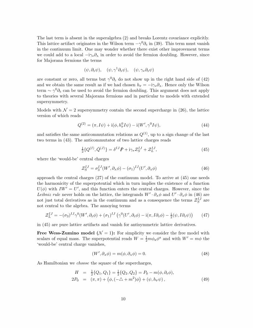
the eigenvalues

λk(0) = ±√

m2 + sin2(pk)

with multiplicity 4 and

λk(1) = ±√

m2 + 4(1 +m) sin2(12pk)

with multiplicity 2. This should be com-pared with the eigenvalues on the contin-

uous interval of ’length’ N ,

λk = ±√

m2 + p2k (58)

with multiplicity 2. One can show that forα greater then α+ or less then α−, where

4α± = ±(√

m2 + 8∓m)

,

all eigenvalues have the same multiplicity as in the continuum. In particular, for masslessfermions there are no doublers for α2 > 1/2. However, for α ∈ [α−, α+] some eigenvalueshave multiplicity four. In the above figure we have plotted the positive eigenvalues of hF

for α = 0, 1, α+. For comparison we have depicted the positive eigenvalues of hF for thenonlocal SLAC derivative

(∂SLAC)n 6=n′ = (−)n−n′ π/N

sin(π(n− n′)/N

) and (∂SLAC)nn = 0. (59)

Despite being nonlocal the SLAC derivative has many advantages as compared to thelocal operators ∂R, ∂L or ∂R+L: it is antisymmetric such that for massless fermions chiralsymmetry is preserved. By construction the 2N real eigenvalues of hF = −iγ∗∂SLAC+γ

0mare identical to the 2N lowest eigenvalues of the continuum operator on the interval of‘length’ N , (58). For this reason ∂SLAC has been called ideal lattice operator in theliterature. We do not expect that unwanted nonlocal counterterms [30] are requiredfor the two-dimensional supersymmetric Wess-Zumino models. This is certainly thecase for the finite models with extended supersymmetry. For the model with N = 1supersymmetry the same should be true since it does not contain gauge fields whichcouple to high momentum modes at the edge of the Brillouin zone. Indeed, in [31] is hasbeen claimed that ∂SLAC approaches an ultra-local operator when N tends to infinity,except for a border matrix. In the appendix we give a detailed analysis of this interestingoperator.

13

3.2 On the Quality of Lattice Derivatives in Supersymmetric QM

It is enlightening to retreat to quantum-mechanical systems and study the supercharges

Q =

(0 AA† 0

)

, with A = ∂ +W, A† = ∂† +W, (60)

and in particular the quality of lattice approximations for different lattice derivatives ∂in A. The supercharge squares to

Q2 =

(AA† 00 A†A

)

, (61)

with isospectral discretized Schrodinger operators

AA† = ∂∂† + ∂W +W∂† +W 2

A†A = ∂†∂ + ∂†W +W∂ +W 2. (62)

They have identical spectra, up to possible zero modes. If the Leibniz rule held on thelattice, if ∂ was antisymmetric and if we could replace ∂W by W ′ +W∂, then we wouldfind the super-Hamiltonian of supersymmetric quantum mechanics in the continuum,

H =

(∂∂† +W ′ +W 2 0

0 ∂†∂ −W ′ +W 2

)

. (63)

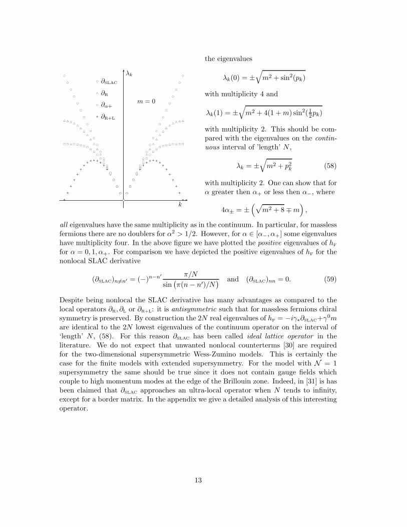
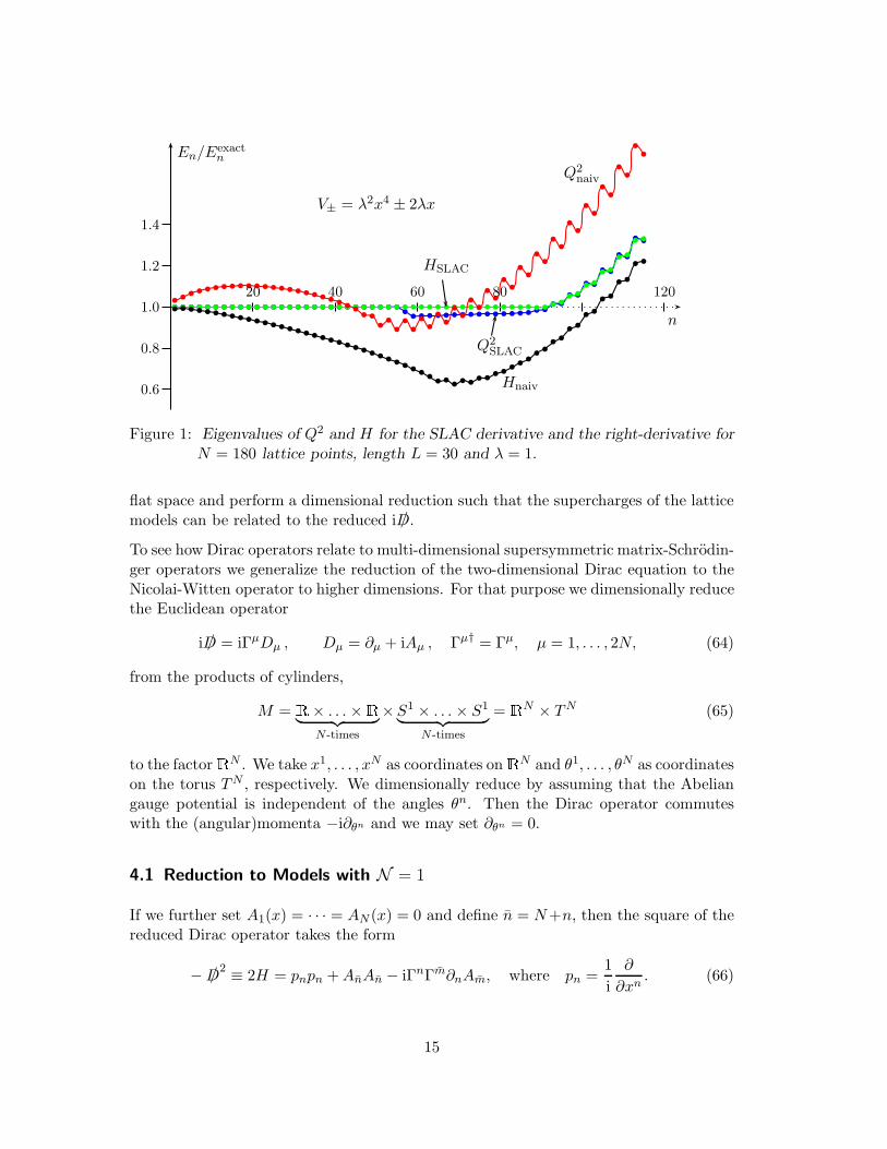
The difference between Q2 and H is the analog of the last two terms in (43) and thedifference in their spectra is a good measure for the suitability of the chosen latticederivative as regards supersymmetry and the speed with which the continuum limit isapproached. In the following figure we have plotted the eigenvalues of Q2 and H for∂ = ∂SLAC, denoted by Q2

SLAC and HSLAC and for ∂ = ∂R, denoted by Q2naiv and Hnaiv.

We took the superpotentialW = λx2 which gives rise to the supersymmetric anharmonicoscillator.

The lowest 57 eigenvalues of Q2 and H are almost identical for the SLAC derivatives andthe lowest 90 eigenvalues of HSLAC agree with the exact values (calculated on a muchfiner grid). These results clearly demonstrate the high precision of the SLAC derivativein low-dimensional supersymmetric systems. It does not matter whether we discretisethe supercharge or the super-Hamiltonian as long as we choose the SLAC derivative.After this detour to quantum mechanics we now return to supersymmetric field theories.

4 From the Dirac Operator to the Lattice N = 1 WZ Model

In this section we relate the supercharges and Hamiltonians of two-dimensional Wess-Zumino models on a spatial lattice to suitable Dirac operators. We shall use the resultsin [32] on the (extended) supersymmetries of i /D in arbitrary dimensions, specialized to

14

n

En/Eexactn

V± = λ2x4 ± 2λx

b b b b b b b b b b b b b b b b b b b b b b b b b b b b

b

b

b

b

b

b

b

b

b

b

b b

b

b

b

b

b

b

b

b

b

b

b

b

b

b

b

b

b

b

b b b b b b b b b b b b b b b b b b b b b b b b b b b b b b b b b b b b b b b b b b

b

b

b

b

b

b

b

b

b

b

b

b

b

b

b

b

b

b

b

b

b

b

b

b

b b

b

b

b

b

b

b

b

b

b

b

b

b

b

b

b

b

b

b

b

b

b

b

b

b

b

b

b

b

b

b

b

b

b

b

b

b

b

b

b

b

b

b

b

b

b

b

b

b

b

b

b

b

b

b

b

b

b

b

b

b

b

b

b

b

b

b

b

b

b

b

b

b

b

b

b

b

b

b

b

b

b

b

b

b

b

b

b

b

b

b

b

b

b

b

b

b

b

b

b

b

b

b

b

b

b

b

Q2SLAC

HSLAC

Q2naiv

Hnaiv

20 40 60 80 120

0.8

0.6

1.0

1.2

1.4

Figure 1: Eigenvalues of Q2 and H for the SLAC derivative and the right-derivative for

N = 180 lattice points, length L = 30 and λ = 1.

flat space and perform a dimensional reduction such that the supercharges of the latticemodels can be related to the reduced i /D.

To see how Dirac operators relate to multi-dimensional supersymmetric matrix-Schrodin-ger operators we generalize the reduction of the two-dimensional Dirac equation to theNicolai-Witten operator to higher dimensions. For that purpose we dimensionally reducethe Euclidean operator

i /D = iΓµDµ , Dµ = ∂µ + iAµ , Γµ† = Γµ, µ = 1, . . . , 2N, (64)

from the products of cylinders,

M = R× . . . ×R︸ ︷︷ ︸

N-times

×S1 × . . . × S1︸ ︷︷ ︸

N-times

= RN × TN (65)

to the factorRN . We take x1, . . . , xN as coordinates onRN and θ1, . . . , θN as coordinateson the torus TN , respectively. We dimensionally reduce by assuming that the Abeliangauge potential is independent of the angles θn. Then the Dirac operator commuteswith the (angular)momenta −i∂θn and we may set ∂θn = 0.

4.1 Reduction to Models with N = 1

If we further set A1(x) = · · · = AN (x) = 0 and define n = N+n, then the square of thereduced Dirac operator takes the form

− /D2 ≡ 2H = pnpn +AnAn − iΓnΓm∂nAm, where pn =

1

i

∂

∂xn. (66)

15

Note that the reduced operator H contains no first-derivative terms. It can be identifiedwith the Hamiltonian of a two-dimensional N = 1 WZ-model on a spatial lattice, if weset

xn = φ(n), pn = π(n) and

(Γn

Γn

)

=√2ψ(n). (67)

It follows with (17) that (ψ, γ0ψ) = −iΓnΓn holds true. If we further assume that thenon-vanishing components of Aµ have the form

An = −(∂†φ)(n) +W ′(φ(n)) with ∂† = ∂S − ∂A, (68)

then we find

− 1√2i /D = (π, ψ1) + (W ′, ψ2)

︸ ︷︷ ︸

A0

−(φ, ∂ψ2)︸ ︷︷ ︸

A1

= Q(1)1 (69)

with Q(1) in (40). We conclude that the Hamiltonian reads

H = P0 + (W ′, ∂Aφ)− (W ′, ∂Sφ), (70)

with P0 from (42). Thus we have proved that the super-Hamiltonian of the N = 1Wess-Zumino model on a lattice with N sites is just the square of the Dirac operator in2N dimensions, dimensionally reduced from R

N × TN to RN .

4.2 Ground State of the Free Model

For the massive non-interacting model we have 2W = mφ2. The corresponding Hamil-tonian is the sum of two commuting operators, of the bosonic part

HB = 12 (π, π) +

12(φ,A

2φ), A2 = −+m∂S +m2, (71)

and the fermionic one

HF = 12(ψ, hFψ), hF = −iγ∗∂A + γ0(m− ∂S). (72)

We assume that the parameters are such that A2 is positive. Near the continuum limitthis is always the case if the physical mass is positive. The ground state wave function(al)of the supersymmetric Hamiltonian factorizes,

Ψ0 = ΨBΨF with HBΨB = EBΨB and HFΨF = EFΨF.

We choose the field representation for the scalar field, such that

π(n) =1

i

∂

∂φ(n)and ΨB = ΨB(φ). (73)

16

The bosonic factor ΨB is Gaussian

ΨB = c · exp(−1

2(φ,Aφ))

and EB = 12 trA. (74)

Here A is the positive root of the positive and Hermitian A2 in (71). For the family ofoperators in (55) the trace of A is just half the sum of the positive eigenvalues in (57).

To find ΨF we introduce the (two-component) eigenfunctions vk of hF with positiveeigenvalues. Since the Hermitian matrix hF is imaginary the vk cannot be real and wehave

hFvk = λkvk ⇐⇒ hFvk = −λkvk (λk > 0). (75)

The eigenvectors are orthogonal with respect to the Hermitian scalar product,

(vk, vk′) =∑

n,α=1,2

vkα(n)vk′α(n) = δkk′ and (vk, vk′) = 0. (76)

Now we expand the Majorana spinors in terms of this orthonormal basis,

ψ(n) =

N∑

k=1

(

χkvk(n) + χ†kvk(n)

)

, where χk = (vk, ψ), χ†k = (vk, ψ) (77)

are one-component complex objects with anticommutation relations

χk, χk′ = 0 and χk, χ†k′ = δkk′. (78)

Inserting the expansion (77) into HF yields

HF = 12

∑

k:λk>0

λk

(

χ†kχk − χkχ

†k

)

. (79)

It follows that the ground state of HF is the Fock vacuum which is annihilated by allannihilation operators χ1, . . . , χN and has energy

EF = −12

∑

k:λk>0

λk. (80)

Since h2F= 12 ⊗A2 we conclude, that the positive eigenvalues of hF are identical to the

eigenvalues of A such that

E = EB + EF = 0.

Since Ψ0 is normalizable for A > 0 we see that the Hamiltonian admits a supersymmetricground state for all choices of the lattice derivative ∂, provided A is positive.

17

4.3 Ground State for Strong Coupling

In the extreme case of very strong self-coupling of the scalar field we may neglect thederivative term in the supercharge (69) [9]. Then Q andH are the sum of N identical andcommuting quantum mechanical operators, each defined on a given lattice site. Hence,the ground state is a product state, Ψ0(φ) = ⊗nψ0(φn). The operators on a fixed lattice

site read

Q(1)1 =

1

iψ1

∂

∂φ+ ψ2W

′(φ) and H = − ∂2

∂φ2+W ′2 − iψ1ψ2W

′′. (81)

A normalizable zero-energy state is annihilated by Q(1)1 ,

ψ0(φ) = e−iψ1ψ2W (φ)ω0, (82)

where ω0 is a constant two-component spinor. It is well-known [33] and follows at oncefrom (82) that supersymmetry is unbroken if p in

W =1

pλφp +O(φp−1), λ 6= 0, (83)

is even and it is broken if p is odd. Note that −iψ1ψ2 is Hermitian and has eigenvalues±1 and that for even p the state ψ0 is normalisable if

i sign (λ)ψ1ψ2ω0 = ω0 or (ψ1 − i sign (λ)ψ2)ω0 = 0.

To summarize, for even p the N = 1 Wess-Zumino model on the spatial lattice hasalways exactly one normalizable zero mode in the strong-coupling limit. For λ > 0 thisproduct state has the form

Ψ0(φ) = exp

(

−N∑

n=1

W (φn)

)

Ω0,(ψ1(n)− iψ2(n)

)Ω0 = 0, ∀ n. (84)

In particular, for φ4-models supersymmetry is broken in the strong-coupling limit where-as it is unbroken for φ6-models.

5 From the Dirac Operator to the Lattice N = 2 WZ Model

It is known, that on flat spacetime the Euclidean Dirac operator admits two supersym-metries if the field strength commutes with an antisymmetric and orthogonal matrix I,which defines a complex structure [32]. The two real supercharges

Q1 =1√2i ΓµDµ and Q2 =

1√2i IµνΓ

νDν (85)

18

form the superalgebra

12Qi, Qj = δijH. (86)

They can be combined to a nilpotent complex charge

Q =1√2(Q1 + iQ2) (87)

and its adjoint Q†, in terms of which the supersymmetry algebra takes the form

H = 12Q,Q†, Q2 = Q†2 = 0 and [Q,H] = 0. (88)

To obtain N = 2 lattice models on N sites we consider the Dirac operator on

M = R× . . .×R︸ ︷︷ ︸

2N-times

×S1 × . . .× S1︸ ︷︷ ︸

2N-times

= R2N × T 2N (89)

in contrast to the 2N -dimensional space in (65). Since the field strength commutes withthe complex structure I it is very convenient to introduce the corresponding complexcoordinates on M ,

zn = xn + ixn = xn + iθn, n = 2N + n, n, n ∈ 1, . . . , 2N, (90)

and fermionic annihilation and creation operators,

ψn = 12

(Γn + iΓn

), ψ†n = 1

2

(Γn − iΓn

)with ψn, ψ†m = δmn. (91)

The condition that Fµν commutes with the complex structure I implies the existence ofa real superpotential χ(z, z), such that [32]

Q = 2ie−χ

(2N∑

n=1

ψn∂

∂zn

)

eχ.

5.1 Reduction to Models with N = 2

Again we perform a dimensional reduction by assuming that χ does not depend on thecompact variables θn,

χ = χ(x1, . . . , x2N

)(92)

and that the angular momenta ∂θn vanish. In the sector with vanishing angular momentathe complex charge simplify to

Q = e−χQ0eχ, where Q0 = i

2N∑

n=1

ψn∂

∂xn, (93)

19

since the complex zn-derivative becomes the real xn-derivative in this sector. Thisdimensional reduced supercharge and its adjoint generate the superalgebra (88) withsupersymmetric matrix-Schrodinger operator

H = 12Q,Q† = −1

2∆+ 12(∇χ,∇χ) + 1

2∆χ︸ ︷︷ ︸

HB

−∑

ψn†χ,nmψm

︸ ︷︷ ︸

HF

. (94)

For example, for χ = −λr this is just the Hamiltonian of the supersymmetrized Hydrogenatom which has been introduced and solved in [34]. It is evident from the representations(93) and (94) that Q decreases and Q† increases the eigenvalue of the number operator

N =∑

ψn†ψn (95)

by one and H commutes with N . The eigenvalues of N are 0, 1, . . . , 2N .

As before, we interpret the 2N coordinates xn and annihilation operators ψn as valuesof two scalar and one Dirac field on a one-dimensional lattice with N lattice sites. Moreprecisely, we make the following identifications for n = 1, 2, . . . , N ,

φ(n) =

(x2n−1

x2n

)

, π(n) =

(p2n−1

p2n

)

,

ψ(n) =

(ψ2n−1

ψ2n

)

, ψ†(n) =

(ψ† 2n−1

ψ†2n

)

. (96)

The free supercharge (93) takes the form

Q0 = i

N∑

n=1

ψ(n)∂

∂φ(n), Q†

0 =

N∑

n=1

ψ†(n)∂

∂φ(n). (97)

The remaining task is to find a superpotential χ giving rise to interacting lattice Wess-Zumino models. Since χ should be real we use a representation for the two-dimensionalγ-matrices such that iγ∗ and γ0 are real,

γ0 = σ3, γ1 = iσ1, γ∗ = −σ2, (98)

in order to obtain a real Dirac-Hamiltonian,

hmF

= −iγ∗∂ +mγ0 =

(m ∂−∂ −m

)

.

As explained above, ∂ need not be anti-Hermitian in which case we take

hmF

=

(m ∂∂† −m

)

= −iγ∗∂A +mγ0 − iγ1∂S with (hmF)2 = (−+m2)12, (99)

such that hmFis real and Hermitian. Note that the term containing ∂S is not a momentum

dependent mass term as in (39). We have been lead to a different type of Wilson term

20

as compared to the N = 1 model since we have chosen a different representation forthe γ-matrices. The earlier Majorana representation (17) is not useful in the presentcontext, since it would lead to a complex χ in (93).

The term HF in (94) must contain the free Dirac-Hamiltonian and this condition implies

− ∂2χm

∂φα(n)∂φβ(n′)= (hm

F)αβ,nn′ , α, β = 1, 2, n, n′ = 1, 2, . . . , N. (100)

Hence we expect that the real function

χm = −12(φ, h

mFφ), (101)

is the superpotential for a N = 2 supersymmetric model. For these models we use thefollowing inner products

(φ, φ) =∑

α,n

φα,nφα,n and (ψ, ψ) =∑

α,n

ψ†α(n)ψα(n), (102)

for scalar doublets and Dirac spinors, respectively. The corresponding supercharge

Q = ie−χm

Q0 eχm

= i∑

n

ψ(n)

(∂

∂φ− hm

Fφ

)

(103)

and its adjoint give rise to the following super Hamiltonian,

HB = −12(π, π) +

12

(φ, (− +m2)φ

), HF = (ψ, hm

Fψ). (104)

Note that the superpotential χm is a harmonic function, χm = 0, and thus there is noconstant contribution to HB. The charges and Hamiltonian act on function(al)s in theHilbert space of the N = 2 lattice models

H = h⊗ · · · ⊗ h︸ ︷︷ ︸

N−times

, where h = L2(R2)⊗C4 (105)

is the Hilbert space for the degrees of freedom on one lattice site.

Now we turn to interacting models by replacing the mass term in

χm = −12(φ, h

0Fφ) +

∑

n

f(φ(n)

), f(φ) = 1

2m(φ22 − φ21),

given by the quadratic harmonic function f , by an arbitrary harmonic function f(φ) ofthe two variables φ1 and φ2,

χ = −12(φ, h

0Fφ) +

∑

f(φ(n)

), where ∆f = 0. (106)

The supercharge and its adjoint are calculated as

Q = e−χQ0eχ and Q† = eχQ†

0e−χ (107)

21

with Q0 and Q†0 from (97). After some algebra one finds for the bosonic part of H =

12Q,Q† the formula

HB = 12(π, π) − 1

2(φ,φ) + 12

(∂f

∂φ,∂f

∂φ

)

+

(∂g

∂φ1, ∂†φ1

)

−(∂g

∂φ2, ∂φ2

)

(108)

where the harmonic functions f and g are the real and imaginary parts of an analyticfunction, such that

∂f

∂φ1=

∂g

∂φ2and

∂f

∂φ2= − ∂g

∂φ1. (109)

For the fermionic part of the Hamiltonian one obtains

HF = (ψ, h0Fψ)−

(ψ, γ0Γ(φ)ψ

), Γ(φ) = f,11(φ)− iγ∗f,12(φ). (110)

The last term contains the Yukawa coupling between scalar and Dirac fields. Note thatthe last two terms in (108) can be rewritten as

Z = −(∂g

∂φ, ∂Aφ

)

+

(∂g

∂φ, σ3∂Sφ

)

. (111)

In the continuum limit the first term on the right becomes a surface term commutingwith the supercharges and the second term, which is a lattice artifact, must vanish. Thusit is natural to set

HB +HF = P0 + Z (112)

and interpret the first term

P0 =12(π, π) − 1

2(φ,∆φ) + (ψ, h0Fψ) +12

(∂f

∂φ,∂f

∂φ

)

−(ψ, γ0Γ(φ)ψ

)(113)

as energy and the second term as ‘would be’ central charge Z in (111). This agrees withour interpretation for solitonic configurations saturating the BPS-bound. To see thatmore clearly we consider the energy of a purely bosonic static solution,

E = P0 = −12(φ,∆φ) +

12

(∂f

∂φ,∂f

∂φ

)

. (114)

From the very construction it is evident, that there is a BPS-bound. One just adds thenon-negative operator HB in (108) to the non-negative operator one gets when changingthe signs of f and g and finds

E ≥ |Z|. (115)

For example, a cubic superpotential f + ig = λφ3/3 leads to a φ4-models with

P0 =12(π, π)− 1

2 (φ,∆φ) + (ψ, h0Fψ) +12λ

2 (φ, φ)2 −(ψ, γ0Γ(φ)ψ

). (116)

22

It contains a scalar and pseudoscalar Yukawa interaction with

Γ(φ) = 2λ(φ1 + iγ∗φ2).

The would-be central charge is cubic in the scalar fields and reads

Z = 2λ(

φ1φ2, ∂†φ1

)

− λ(

φ21 − φ22, ∂φ2

)

. (117)

Before turning to the discussion of the ground state we note, that the conserved numberoperator

N =∑

n

ψ†(n)ψ(n) (118)

leads to a decomposition of the Hilbert space (105) in orthogonal subspaces labelled bythe fermion number,

H = H0 ⊕H1 ⊕ · · · ⊕ H2N−1 ⊕H2N , N∣∣Hp

= p1. (119)

The nilpotent supercharge Q decreases N by one, Q† increases it by one and the super-Hamiltonian commutes with N ,

[N,Q] = −Q, [N,Q†] = Q† and [N,H] = 0. (120)

We call the subspace Hp p-particle sector. The states in the zero-particle sector areannihilated by Q and those in the 2N -particle sector by Q†.

5.2 Ground State of the Free Model

The Hermitian lattice Dirac-Hamiltonian hmF

in (99) is real and can be diagonalized byan orthogonal matrix S,

hmF

= S−1DS, D = diag(d1, d2, . . . , d2N ). (121)

We rotate the field-variables with S,

ξ = Sφ, η = Sψ and η† = Sψ†.

The new fields still obey the standard anticommutation relations, e.g.

η†α(n), ηβ(m) = δαβδnm, (122)

and the transformed supercharges read

Q = iη

(∂

∂ξ−Dξ

)

and Q† = iη†(∂

∂ξ+Dξ

)

(123)

23

and show, that the new degrees of freedom decouple. Hence the ground state must havethe product form

Ψ0 = exp(

−12

∑

|da|ξ2a)

|Ω〉 (124)

and the supercharges act on this state as follows,

QΨ0 = 2i∑

a: da>0

daηaξaΨ0 , Q†Ψ0 = −2i∑

a: da<0

daη†aξaΨ0. (125)

This way we arrive at the following conditions for this state to be invariant,

da > 0 =⇒ ηa|Ω〉 = 0 and da < 0 =⇒ η†a|Ω〉 = 0. (126)

This leads to the unique normalizable ground state (124) with

|Ω〉 =∏

da<0

η†a|0〉. (127)

which is annihilated by the supercharges and hence has vanishing energy. There are Npositive and N negative eigenvalues of hm

Fsuch that the invariant vacuum state lies in

the middle sector HN in the decomposition (119) of the Hilbert space. All fermionicstates with negative energies are filled. This is just the Dirac-sea filling prescription.Note that our result is the lattice version of the continuum result for the ground state,

Ψ0 = exp

(

−12

∫

φα√

−+m2φα

)

|Ω〉.

5.3 Ground States for Strong Coupling

In the strong-coupling limit we may neglect the spatial derivatives such that the super-charges and the Hamiltonian becomes the sum of N commuting operators, each definedon one lattice site [21]. The operators on a given site take the form

Q = iψ (∇+∇f) , H = −12+ 1

2(∇f,∇f)− ψ†f ′′ψ. (128)

Now we explicitly construct the ground state for the harmonic superpotential

f(φ) =λ

pReφp, φ = φ1 + iφ2 = reiθ, (129)

which gives rise to a supersymmetric anharmonic oscillator on the Hilbert space h =L2(R

2)×C4. The bosonic part of H reads

HB = −12+ V with V = 1

2λ2r2p−2, (130)

24

and its fermionic part

HF = λ(p−1)ψ†

(−Reφp−2 Imφp−2

Imφp−2 Reφp−2

)

ψ (131)

It is useful to note that H commutes with the operator

J = L+ S, S = −sψ†σ2ψ, s = 12(p− 2) (132)

and that the ground state must reside in the two-dimensional sector with particle numberN = ψ†ψ = 1, since the restriction of HF to the zero- and two-particle sectors vanishand HB > 0. The one-particle sector is spanned by the following two eigenstates of S,

|↑〉 =(

ψ†1 − iψ†

2

)

|0〉 and |↓〉 =(

ψ†1 + iψ†

2

)

|0〉 (133)

with eigenvalues 1 and −1, respectively. Here |0〉 denotes the Fock-vacuum which isannihilated by the annihilation operators ψα. Diagonalising J in this sector leads to theansatz

ψ0j(φ) = Rj+(r)ei(j−s)θ |↑〉+Rj−(r)e

i(j+s)θ |↓〉, (134)

where the J-eigenvalue j is integer for even p and half-integer for odd p. Inserting intoQψj = Q†ψj = 0 yields the following coupled system of first order differential equationsfor the radial functions

R′j±(r)−

s∓ j

rRj±(r) + λrp−1Rj∓(r) = 0.

The square integrable solutions are Bessel functions

Rj±(r) = c rp−1K 12± j

p

(λp r

p)

with j ∈ −s,−s+ 1, . . . , s− 1, s. (135)

The number of supersymmetric ground states of the models with φ2p−2 self-interactionis just p− 1. The (p− 1)N normalizable invariant eigenstates are

Ψ0,j1,...,jN =

N⊗

n=1

ψ0jn(φn) ∈ h1 × · · · × hN . (136)

For example, for the N = 2 model with φ4 interaction there exist 2N normalizable zeromodes in the strong-coupling limit. This number diverges in the thermodynamic limit.On the other hand, there is exactly one normalisable zero mode when one switches offthe self-interaction. This discrepancy between the number of supersymmetric groundstates in the weak and strong-coupling regimes becomes even more puzzling when onetakes into account certain rigorous theorems on the stability of such states under analyticperturbations discussed in the following section. The zero modes in (136) with radialfunctions (135) have been constructed previously in [21, 33] and [35].

25

6 From Strong to Weak Couplings

6.1 Perturbation Theory and Zero Modes

Let us recall a well known result for perturbation theory of zero modes in supersymmetricquantum mechanics [33]. We consider the N = 1 case and denote the single Hermitiansupercharge by Q0,

Q20 = H0, Γ, Q0 = 0, Γ† = Γ, Γ2 = 1. (137)

In addition, we define the projection operators

P± = 12(1± Γ) (138)

which project on the ±1 eigenspaces of Γ. These eigenspaces are denoted by HB/F. Inthe following we assume that there are no zero modes in HF and at least one zero modeΨ0 in the bosonic sector HB. We perturb the operator Q0 by an operator ǫQ1 with realparameter ǫ, Q(ǫ) = Q0 + ǫQ1, where Q1,Γ = 0. We want to solve the eigenvalueequation

Q(ǫ)Ψ(ǫ) = λ(ǫ)Ψ(ǫ),

with λ(0) = 0 and Ψ(0) = Ψ0. We consider the following formal power series in ǫ,

Ψ(ǫ) = Ψ0 +∞∑

k=1

ǫkΨk, λ(ǫ) =∞∑

k=1

ǫkλk.

Proposition: Under the assumptions above one has λ(ǫ) = 0 and ΓΨ(ǫ) = Ψ(ǫ) in thesense of formal power series.

Proof by induction: To order ǫ0 the proposition holds. Let us assume it holds up toorder ǫj−1. To order ǫj we obtain the equation

Q0Ψj +Q1Ψj−1 = λjΨ0. (139)

Taking the scalar product with Ψ0 yields

λj = (Ψ0, Q1Ψj−1).

Since Γ squares to 1 and anticommutes with the perturbation we find

λj = (Γ2Ψ0, Q1Ψj−1) = −(ΓΨ0, Q1ΓΨj−1) = −(Ψ0, Q1Ψj−1) = −λj ,

which proves that λj = 0. Furthermore, with

Q0ΓΨj = −ΓQ0Ψj = ΓQ1Ψj−1 = −Q1Ψj−1 = Q0Ψj ,

26

we conclude

Q0P−Ψj = 0,

where we used the projection operator P− introduced in (138). As P−Ψj is a zero modeof Q0 it follows by assumption that it resides in HB. But as P− projects onto HF,we conclude P−Ψj = 0 or Ψj ∈ HB. This then proves our statement. Note that thestatement has been proved in the sense of formal power series only. In case λ(ǫ) is notanalytic at ǫ = 0 the result above maybe misleading.

6.2 The N = 1 Case

In what follows, we compare the strong-coupling results with the usual perturbationtheory around minima of the potential.

In the case deg(W ) = p even, supersymmetry is never broken, neither in the strong-coupling limit nor in perturbation theory. For even p there is at least one minimum ofthe potential V = 1

2(W′)2 with V = 0. The quadratic approximation of the potential at

the critical points yields for each minimum one normalizable zero mode similar to theground state of the free model. In contrast to the strong-coupling limit there may bemore than one perturbative zero mode, but they always come in an odd number. Thedifference of bosonic and fermionic zero modes is ±1 as in the strong-coupling limit.

In the case deg(W ) = p odd, the difference between the strong-coupling limit and per-turbation theory is more severe. Supersymmetry is broken in the strong-coupling limitbut it may be unbroken in perturbation theory. Let us consider an explicit example,

W (φ) =g22φ3 + g0φ. (140)

Perturbation theory for g0 < 0 predicts one bosonic and one fermionic zero mode (un-broken supersymmetry), and broken supersymmetry for g0 > 0. The strong-couplinglimit states that supersymmetry is broken for all g0.

In Appendix B.1 we provide the rigorous proof that λA1 with A1 given in (69) is ananalytic perturbation of A0 in (69). This implies that all eigenvalues are analytic func-tions of the parameter λ. Assume now that in a finite range of the parameter λ thereis a ground state with energy zero. As an analytic function which vanishes in somefinite range is identically zero, the number of zero modes changes at most at isolatedpoints of the parameter space of λ. Furthermore, in the strong-coupling limit, we haveeither bosonic or fermionic zero modes. In subsection 6.1 we have proved that under thisassumption a zero mode always remains a zero mode. We conclude that, generically,the number of zero modes is given by the number of zero modes in the strong-couplinglimit. Generically, since for certain discrete values of λ the number of zero modes couldbe enhanced. Moreover, as the index also depends analytically on the parameter λ, weare able to calculate this index in the strong-coupling limit.

27

In the continuum and infinite-volume limit these arguments may break down, as theestimates necessary for proving analyticity (see Appendix B.1) may not be valid anymore.In the unbroken case we can definitely conclude that the theory is still unbroken in thecontinuum and infinite-volume limit. Suppose we know that for any finite lattice thereis at least one ground state with zero energy. As the limit of zero is again zero thismode survives in the limit. In the case of broken supersymmetry a non-zero energyeigenstate may become a zero mode in the continuum and infinite-volume limit, andsupersymmetry may get restored in this limit although it is broken for all finite lattices.

Indeed, for negative g0 in our example above, the scalar field has a non-vanishing vacuumexpectation value and therefore the fermionic field ψ acquires a non-zero mass. As thereis no massless Goldstone fermion, supersymmetry has to be unbroken in this case [3].

Let us summarize. On a finite lattice, the strong-coupling limit gives the correct number

of zero modes of the full problem. There is only one zero mode in the case wheredeg(W ) = p is even, and otherwise there is no zero mode. Variations of the parametersin the superpotential of power less than p do neither change the number of zero modesnor the index. For example, in the model with superpotential given in (140), it isimpossible to have two phases of broken and unbroken supersymmetry (depending onthe value of the parameter g0) on a finite lattice. The numerical simulations in [25] maybe interpreted as hinting towards such a phase transition in the continuum theory.

6.3 The N = 2 Case

Similar to the case N = 1, we prove in Appendix B.2 that the index in the strong-coupling limit is the same as for the full problem. This implies that we have at least(p − 1)N zero modes for the theory on finite lattices. For the continuum theory in afinite volume, it was shown using methods of constructive field theory that the N = 2Wess-Zumino model is ultraviolet finite and that the index is given by p − 1 [24]. Thisseems to be in contradiction with our result, as the (p − 1)N zero modes exist for allfinite lattices and, by the same arguments as for the N = 1 model, remain zero modesin the continuum limit.

We suggest the following solution for this problem. Remember that our lattice Hamilto-nian H contains not only the discretized version of the continuum Hamiltonian P0 butalso the central charge Z, i.e.

H = P0 + Z. (141)

Furthermore, both P0 and Z contain the lattice derivative which couples fields at differentlattice sites. If we choose in the strong-coupling limit a zero mode that varies from latticepoint to lattice point, both P0 and Z may become very large but will, nevertheless, addup to zero. In the continuum limit the energy P0 may be infinite in which case thisrapidly varying zero mode is only a lattice artifact. On the other hand, if we choosethe same zero mode for each lattice site, then P0 as well as Z should be zero in the

28

continuum limit. Thus, there are exactly p − 1 such modes. We are planning to testthis proposal in a perturbative calculation of P0 and Z. The results will be presentedelsewhere.

7 Conclusions

In this paper we have related Dirac operators defining supersymmetric quantum me-chanical systems in high-dimensional spaces [32] to Wess-Zumino models on a spatiallattice in 1 + 1 dimensions. After a very particular dimensional reduction the squareof i /D can be identified with the super-Hamiltonians of latticized Wess-Zumino models.This way we discovered a natural connection between discretized supersymmetric fieldtheories and supersymmetric quantum mechanics.

We have recalled the continuum formulation of Wess-Zumino models and discussed theirlattice versions. For the case of simple (N = 1) and extended (N = 2) supersymmetry,we have derived the corresponding Dirac operators. Furthermore, all ground states forthe free massive models and the interacting theories in the limit of strong coupling havebeen constructed.

Different realizations of lattice derivatives have been discussed and their properties – inparticular from the point of view of supersymmetric quantum mechanics – have beenanalyzed. Our results on the number of zero modes do not depend on the particularlattice derivative, as long as some mild assumptions are fulfilled.

Employing powerful theorems from functional analysis we were able to relate the strongand weak coupling regions. For N = 1 it turns out that generically the number of zeromodes is determined by the strong-coupling limit. There is a single (no) zero mode, ifthe degree of the superpotential is even (odd). For N = 2 we find at least (p− 1)N zeromodes, where p is the degree of the superpotential and N the number of lattice sites.This number is far off the correct continuum result, which predicts p− 1 zero modes, aserious problem which has been observed earlier in [21].

We have explained this paradox as follows: the lattice Hamiltonian H does not only con-tain the continuum Hamiltonian P0 but also additional terms which (for antisymmetriclattice derivatives) are to be interpreted as a lattice version of the central charge Z. Onthe lattice, P0 and Z cancel pairwise for the huge number of zero modes under discus-sion, even though neither P0 nor Z is zero in the continuum limit, except for exactlyp− 1 of the modes.

Our Dirac operators clearly deserve further studies. For instance, the application of(standard) index theorems to the case at hand should reveal new information about thefield theories. We also plan to extend our results to Dirac operators on curved manifolds,which can be reinterpreted as nonlinear σ-models from the field theory point of view.

29

Acknowledgements

We thank Hans Triebel for very useful discussions on aspects of functional analysis andFalk Bruckmann and Ivo Sachs for useful conversations. A.K. acknowledges support bythe Studienstiftung des Deutschen Volkes.

A The SLAC Operator

In this appendix we introduce and discuss the nonlocal SLAC derivative. It can be usedto define chiral fermions without fermion-doubling.

First we consider real valued scalar fields on the spatial lattice. They maybe interpretedas wave functions of a quantum mechanical system with Hilbert space RN , equippedwith the scalar product

(φ, χ) =

N∑

n=1

φ(n)χ(n).

Although the fields are real it is useful to embed them in the space of complex valuedlattice fields. For a normalised function we interpret |φ(n)|2 as probability for finding the’particle’ at the lattice site n. Expectation values of functions of the ’position’ operatorn are

〈f(n)〉φ =∑

φ(n)f(n)φ(n). (142)

We want to derive a similar formula for expectation values of functions of the momentumoperator. For that aim we Fourier transform the wave function as follows

φ(pk) =1√N

N ′

∑

n=−N ′

e−ipk nφ(n), where N ′ = 12 (N−1), pk =

2π

Nk. (143)

The inverse Fourier transformation reads

φ(n) =1√N

N ′

∑

k=−N ′

eipk nφ(pk), n = −N ′, . . . , N ′. (144)

We have chosen the symmetric summation to end up with a real difference operator. Forperiodic fields nmust be integer and this is the case for space lattices with an odd number

of sites. For a normalized φ the Fourier transform φ is normalized as well and we mayinterpret |φ(pk)|2 as probability for finding the ’momentum’ pk. With this interpretationwe obtain

〈f(p)〉φ =

N ′

∑

k=−N ′

f(pk) |φ(pk)|2 =∑

nn′

φnf(p)nn′φn′ (145)

30

with matrix elements

f(p)nn′ =1

N

N ′

∑

k=−N ′

eipk(n−n′)f(pk).

With the help of the generating function

Z(x) =

N ′

∑

k=−N ′

eipkx =sin(πx)

sin(πx/N), (146)

we can calculate all matrix elements of f(p). Now we are ready to define the real,nonlocal and antisymmetric lattice operator ∂SLAC = ip. The matrix elements are

f(∂SLAC)nn′ =1

Nf

(d

dx

)

Z(x)∣∣∣x=n−n′

. (147)

As expected ∂SLAC is a Toeplitz matrix with elements

(∂SLAC)nn′ = (−)n−n′ π/N

sin(π(n− n′)/N

) , for n 6= n′, (148)

and the elements on the diagonal vanish, (∂SLAC)nn = 0.

B Analyticity of Perturbation

In the following we consider operators on the Hilbert space

H = L2(Rd,ddx)⊗CD (149)

for D ∈ N with norm

‖f‖2 =D∑

i=1

‖fi‖2L2, f = (f1, . . . , fD) ∈ H. (150)

Here, ‖ · ‖L2denotes the familiar L2-norm.

B.1 The N = 1 Case

For the Wess-Zumino model on the lattice with N = 1 supersymmetry we take D = 2N ,d = N (N = number of lattice points) and consider the (unperturbed) operator (69)

A0 =

N∑

n=1

(−iψ1(n)∂n + ψ2(n)W

′(xn)). (151)

31

We recall that W is a polynomial of degree deg(W ) = p > 1 and ψα(n) are HermitianD ×D−matrices obeying the Clifford algebra

ψα(n), ψβ(n′) = 2δαβδ(n, n′), α, β = 1, 2, n, n′ = 1, 2, . . . , N. (152)

The operator A0 with domain of definition

D(A0) = C∞c (RN )⊗CD

is essentially self-adjoint, where we write C∞c (RN ) for the C∞-functions with compact

support in RN . A simple calculation using (152) shows

(A0)2 =

∑

n

(−∂n∂n +W ′(xn)W

′(xn)− iψ1(n)ψ2(n)W′′(xn)

).

Closure of the Operator A0

To determine the closure A0 of the operator A0 we have to find the closure of its domainD(A0) with respect to the norm

‖f‖2A0,a = a‖f‖2 + ‖A0f‖2, a > 0. (153)

Note that these norms are equivalent for all a > 0. Using the abbreviation

ρp = 1 + |x|p−1, (154)

we can prove the following

Lemma: There exist constants a, b1, b2 > 0 such that

‖f ′‖2 + b1‖ρpf‖2 ≤ ‖f‖2A0,a ≤ ‖f ′‖2 + b2‖ρpf‖2 (155)

holds for all f ∈ D(A0).

In the Lemma we used the short hand notation ‖f ′‖2 =∑m ‖∂mf‖2.Proof: First, we show that only the degree deg(W ) = p is important for terms like∑

n ‖W ′(xn)f‖2 with f ∈ D(A0). Indeed, we find

∑

n

‖W ′(xn)f‖2 ≤ Na1‖ρpf‖2, a1 =

∥∥∥∥

W ′(xn)

ρp

∥∥∥∥

2

∞

, (156)

where ‖ · ‖∞ denotes the supremum norm. The factor N arises from the sum over n, asa1 does not depend on n. Similar we obtain

‖ρpf‖2 =

∥∥∥∥∥

ρp√

1 +∑

nW′2(xn)

√

1 +∑

W ′2(xn) f

∥∥∥∥∥

2

≤ a2

(

‖f‖2 +∑

‖W ′(xn)f‖2)

, a2 =

∥∥∥∥∥

ρp√

1 +∑W ′2(xn)

∥∥∥∥∥

2

∞

. (157)

32

Now, it is easy to prove the second inequality in (155),

a‖f‖2 + ‖A0f‖2(156)≤ ‖f ′‖2 + a‖f‖2 +Na1‖ρpf‖2 +

∑

n

‖f‖ ‖W ′′(xn)f‖

≤ ‖f ′‖2 + (a+Na1 +Na3)︸ ︷︷ ︸

b2

‖ρpf‖2, (158)

with a3 =∥∥∥W ′′(xn)ρp

∥∥∥∞. We used that the matrix-norm of ψα(n) is one, since its eigen-

values are ±1. In the last inequality we made use of ‖f‖ ≤ ‖ ρpf‖ which holds for allf ∈ D(A0).

The other inequality in (155) is more difficult to prove. With (157) we get

a‖f‖2 + ‖A0f‖2 ≥ ‖f ′‖2 + 1

a2‖ρpf‖2 + (a− 1)‖f‖2 −

∑

‖f‖ ‖W ′′(xn)f‖. (159)

In order to obtain a positive constant b1 in our lemma we must be rather careful withour estimates for the last term in (159). We introduce a ball of radius R and split f intotwo parts, f = f<+ f>, where f< has its support inside the ball f> outside the ball. Weobtain

∑

n

‖f‖ ‖W ′′(xn)f‖ =∑(

‖f<‖ ‖W ′′(xn)f<‖+ ‖f>‖ ‖W ′′(xn)f>‖), (160)

where the terms containing both f< and f> vanishes. Let us now consider the two termsseparately. First, we obtain

∑

‖f>‖ ‖W ′′(xn)f>‖ ≤ Na4(R)‖ρpf‖2, a4(R) =

∥∥∥∥

W ′′(xn)

ρp

∥∥∥∥∞,>

, (161)

where we have introduced the supremum norm ‖ · ‖∞,> = sup|x|>R| · |. For large R wehave a4(R) ∼ 1/R such that a4 gets arbitrarily small for big balls. Second, we obtain

∑

‖f<‖ ‖W ′′(xn)f<‖ ≤ Na5(R)‖f‖2, a5(R) = ‖W ′′(xn)‖∞,<, (162)

with ‖ · ‖∞,< = sup|x|<R| · |. For R→ ∞ we have a5(R) → ∞. Altogether, we find

a‖f‖2 + ‖A0f‖2 ≥ ‖f ′‖2 + (a− 1−Na5(R)) ‖f‖2 + (1/a2 −Na4(R))︸ ︷︷ ︸

b1

‖ρpf‖2. (163)

In a first step we choose R large enough such that b1 is positive. In a second step wechoose a large such that the constant in front of ‖f‖2 is positive as well. This finishesthe proof of our lemma.

Since all norms

‖f‖2b ≡ ‖f ′‖2 + b ‖ρpf‖2 (164)

33

are equivalent for b > 0, the Lemma implies that these norms are equivalent to thenorms ‖f‖2A0,a

in (153). Therefore, the closure of D(A0) with respect to the norm (153)coincides with the closure with respect to ‖ · ‖b. This closure is given by

D(A0) =f ∈W 1

2 (RN )⊗CD : ‖ρpf‖ <∞

≡W 1

2 (RN , ρ2p)⊗CD. (165)

Here W 12 (R

N ) is the Sobolev space with first weak-derivative in L2.

PerturbationLet us perturb the operator A0 by the operator A1 in (69),

A1 = −N∑

m,n=1

xm (∂)mn ψ2(n). (166)

The operator A1 is self-adjoint with D(A1) = L2(RN , ρ)⊗CD ⊃ D(A0), with ρ-weighted

Lebesgue measure, where ρ(x) = (1 + |x|)2. From the following Lemma we will deriveuseful information about the nature of the perturbation.

Lemma: For all λ ∈ R and arbitrarily small ǫ > 0 there exists a Cǫ > 0 such that

‖λA1f‖ ≤ ǫ‖A0f‖+ Cǫ‖f‖, ∀f ∈ D(A0). (167)

Proof: We prove the inequality for all f ∈ D(A0). Then it holds for all elements in theclosure as well. As before we split f = f< + f>. First, we note

‖λA1f<‖ ≤ |λ|N2a(R) ‖f‖, a(R) = ‖xn‖∞,< ·max|∂mn| : m,n = 1, . . . , N. (168)

For R→ ∞ the constant a(R) tends to infinity. Next, we have

‖λA1f>‖(155)≤ |λ|N2b(R) (c ‖f‖+ ‖A0f‖) ,

b(R) =

∥∥∥∥

xnρp(x)

∥∥∥∥∞,>

·max|∂mn| : m,n = 1, . . . , N (169)

for some positive constant c. For big R the constant b(R) tends to zero. We choose theball big enough such that |λ|N2b(R) = ǫ and set Cǫ = ǫc + |λ|N2a(R). Note that thelatter constant may become huge.

Self-adjointnessWe did prove that A0 is a self-adjoint operator. Clearly λA1 is symmetric on D(A0).Furthermore, (167) shows that λA1 is A0-bounded with relative bound less than one.The famous Kato-Rellich Theorem, see Theorem X.12 in [36], states that under theseconditions the operator

Q1(λ) = A0 + λA1 (170)

is self-adjoint with domain D(A0). We conclude that Q1(λ) is a family of self-adjointoperators with common domain of definition D(A0).

34

Analyticity of EigenvaluesIn the following we prove that Q1(λ) is an analytic family in the sense of Kato for allreal λ. We have seen that Q1(λ) is self-adjoint for real λ. For a self-adjoint and analyticfamily it is known that the eigenvalues depend analytically on the parameter λ, see forexample Theorem XII.13 in [36].

For an arbitrary real λ0 the perturbation λ0A1 is A0-bounded with arbitrary smallrelative bound (167). Then, it is easy to see that A1 is Q1(λ0)-bounded. It followsthat for small ǫ the operators Q1(λ0 + ǫ) form an analytic family of type (A) [36] andtherefore also an analytic family in the sense of Kato. But as λ0 ∈ R is arbitrary, wehaven proved that Q1(λ) is analytic for all real λ.

Actually, the cited Theorem XII.13 [36] above is only valid for isolated eigenvalues withfinite degeneracy or equivalently for eigenvalue in the discrete spectrum. In the followingwe prove that the spectrum of Q1(λ) is discrete by proving this statement for its square,H(λ) = Q1(λ)

2. H(λ) is self-adjoint with domain of definition given by

D (H(λ)) ≡f ∈ D(A0) : Q1(λ)f ∈ D(A0)

= W 22 (R

N , ρ′)⊗CD, ρ′(x) =(1 + |x|2p−2

)2(171)

and it is semibounded

H(λ) ≥ 0. (172)

Such operators possess entirely discrete spectra if and only if its resolvent is a compactoperator, see Theorem XIII.64 in [36]. In the following we prove that H(λ) has compactresolvent for all λ ∈ R.

We must prove that the image of a bounded subset of the Hilbert space, say

f ∈ H : ‖f‖ < 1, (173)

is mapped to a precompact set under the map (H − z)−1 for some z in the resolvent ofH. The image is given by

g ∈ D(H) : ‖(H − z)g‖ < 1. (174)

As earlier we split g into g> and g< and obtain for large enough radii R the inequality‖g‖ ≤ ‖g<‖ + ǫ. For a compact ball B = x ∈ R

N : |x| ≤ R we have Sobolev’sembedding theorem and there is an ǫ-net gj ∈W 2

2 (K, ρ′), j = 1, . . . , Nǫ with ‖g<−gj‖ < ǫ

for one j ∈ 1, . . . , Nǫ. We extend the gj by zero to the region outside the ball andobtain

‖g − gj‖ ≤ 2ǫ (175)

for any g in the image of the unit ball under (H − z)−1 and a specific j ∈ 1, . . . , Nǫ.We conclude that there is a 2ǫ-net of the image and therefore the image is precompact.This completes our proof.

35

Stability of the IndexWe have shown that the eigenvalues are analytic functions of the parameter λ on thewhole real axis. It follows at onces that the index – the difference of bosonic zero modesand fermionic zero modes – is also an analytic function and, as the index only takes oninteger values, is constant.

An alternative and elegant proof of this statement can be given with the help of thetheorem that a relatively compact perturbation does not change the index [37]. Indeed,inequality (167) implies that our perturbation is relatively compact1.

B.2 The N = 2 Case

After the detailed investigation of the N = 1 case we shorten our discussion for N = 2.In what follows we consider the real part of the complex supercharge in (107)

B0 =N∑

n=1

(

−iψ11(n)∂xn − iψ2

1(n)∂yn +2∑

a=1

ψa2 (n)W,a(xn, yn)

)

(176)

in the strong-coupling limit. For N = 2 supersymmetry the ψaα are D-dimensionalHermitian matrices obeying the Clifford algebra, with D = 22N . The function W (x, y)is harmonic and and thus is the real part of an analytic function F (x+iy). As in chapter2 we use the notation W,1 (x, y) = ∂xW (x, y) and W,2 (x, y) = ∂yW (x, y). As domain ofdefinition we take

D(A0) = C∞c (R2N )⊗CD, D = 22N , (177)

such that B0 is essentially self-adjoint. We introduce the potential

K(x, y) =∑

a

W,2a (x, y). (178)

For large radii r only the leading power of W is relevant. Therefore, we may considerthe particular case

W (x, y) =κ

pRe zp (179)

for which we find K(x, y) = κrp−1 → ∞ in all directions for r → ∞.

The perturbation contains the lattice derivative,

B1 =

2N∑

m,n=1

(

xm(∂)mnψ22(n) + ym(∂

†)mnψ12(n)

)

.

Replacing in the estimates for the case with N = 1 supersymmetry the potential W ′(xn)by K(xn, yn) leads to analogous results in the N = 2 case. Again all eigenvalues areanalytic functions of the parameter λ and in particular the index does not depend onthis parameter.1We thank H. Triebel for the proof of this statement.

36

References

[1] C.A.P. Galvao and C. Teitelboim, Classical Supersymmetric Particles, J. Math.

Phys. 21 (1980) 1863.

[2] H. Nicolai, Supersymmetry and Spin Systems, J. Phys. A9 (1976) 1497,P. Salomonson and J.W. van Holten, Fermionic Coordinates and Supersymmetry

in Quantum Mechanics, Nucl. Phys. B196 (1982) 509, F. Cooper, A. Khare andU. Sukhatme, Supersymmetry in Quantum Mechanics, World Scientific, Singapore(2001), G. Junker, Supersymmetric Methods in Quantum and Statistical Physics,Springer-Verlag, Berlin (1996).

[3] E. Witten, Dynamical Breaking of Supersymmetry, Nucl. Phys. B188 (1981) 513.

[4] M.F. Sohnius, Introducing Supersymmetry, Phys. Rept. 128 (1985) 39, J. Wessand J. Bagger, Supersymmetry and Supergravity, Princeton University Press,Princeton (1992), S. Weinberg, The Quantum Theory of Fields. Volume 3:

Supersymmetry, Cambridge University Press, Cambridge (2000).

[5] M.B. Green, J.H. Schwarz, and E. Witten, Superstring Theory. Volume 1:

Introduction, Cambridge University Press, Cambridge (1987), D. Lust andS. Theisen, Lectures on String Theory, Lect. Notes Phys. 346 (1989) 1,J. Polchinski, String Theory. Volume 2: Superstring Theory and Beyond,Cambridge University Press, Cambridge (1998).

[6] N. Seiberg and E. Witten, Electric-Magnetic Duality, Monopole Condensation,

and Confinement in N=2 Supersymmetric Yang-Mills Theory, Nucl. Phys. B426(1994) 19, [hep-th/9407087], Monopoles, Duality and Chiral Symmetry Breaking

in N=2 Supersymmetric QCD, Nucl. Phys. B431 (1994) 484, [hep-th/9408099].

[7] J.M. Maldacena, The Large N Limit of Superconformal Field Theories and

Supergravity, Adv. Theor. Math. Phys. 2 (1998) 231, [hep-th/9711200].

[8] P.H. Dondi and H. Nicolai, Lattice Supersymmetry, Nuovo Cim. A41 (1977) 1.

[9] S. Elitzur, E. Rabinovici and A. Schwimmer, Supersymmetric Models on the

Lattice, Phys. Lett. B119 (1982) 165.

[10] T. Banks and P. Windey, Supersymmetric Lattice Theories, Nucl. Phys. B198(1982) 226.

[11] J. Bartels and J.B. Bronzan, Supersymmetry on a Lattice, Phys. Rev. D28 (1983)818.

[12] I. Montvay, SUSY on the Lattice, Nucl. Phys. Proc. Suppl. 63 (1998) 108,[hep-lat/9709080], M.F.L. Golterman and D.N. Petcher, A Local Interactive

Lattice Model with Supersymmetry, Nucl. Phys. B319 (1989) 307, W. Bietenholz,Exact Supersymmetry on the Lattice, Mod. Phys. Lett. A14 (1999) 51,[hep-lat/9807010].

37

[13] S. Catterall and S. Karamov, A Lattice Study of the Two-Dimensional Wess-

Zumino Model, Phys. Rev. D68 (2003) 014503, [hep-lat/0305002].

[14] I. Montvay, Supersymmetric Yang-Mills Theory on the Lattice, Int. J. Mod. Phys.

A17 (2002) 2377, [hep-lat/0112007].

[15] DESY-Munster-Roma Collaboration, F. Farchioni et. al., The Supersymmetric

Ward Identities on the Lattice, Eur. Phys. J. C23 (2002) 719, [hep-lat/0111008].

[16] V. Rittenberg and S. Yankielowicz, Supersymmetry on the Lattice,CERN-TH-3263.

[17] H.B. Nielsen and M. Ninomiya, Absence of Neutrinos on a Lattice. 1. Proof by

Homotopy Theory, Nucl. Phys. B185 (1981) 20, Absence of Neutrinos on a

Lattice. 2. Intuitive Topological Proof, Nucl. Phys. B193 (1981) 173.

[18] D. Friedan, A Proof of the Nielsen-Ninomiya Theorem, Commun. Math. Phys. 85(1982) 481.

[19] J. Wess and B. Zumino, Supergauge Transformations in Four Dimensions, Nucl.Phys. B70 (1974) 39.

[20] H. Nicolai, On a New Characterization of Scalar Supersymmetric Theories, Phys.Lett. B89 (1980) 341, N. Sakai and M. Sakamoto, Lattice Supersymmetry and the

Nicolai Mapping, Nucl. Phys. B229 (1983) 173.

[21] S. Elitzur and A. Schwimmer, N=2 Two-Dimensional Wess-Zumino Model on the

Lattice, Nucl. Phys. B226 (1983) 109.

[22] S. Catterall and S. Karamov, Exact Lattice Supersymmetry: the Two-Dimensional

N=2 Wess-Zumino Model, Phys. Rev. D65 (2002) 094501, [hep-lat/0108024].

[23] E. Witten and D.I. Olive, Supersymmetry Algebras that Include Topological

Charges, Phys. Lett. B78 (1978) 97.

[24] A. Jaffe, A. Lesniewski, and J. Weitsman, Index of a Family of Dirac Operators on

Loop Space, Commun. Math. Phys. 112 (1987) 75.

[25] M. Beccaria, M. Campostrini, and A. Feo, Supersymmetry Breaking in Two

Dimensions: The Lattice N=1 Wess-Zumino Model, Phys. Rev. D69 (2004)095010, [hep-lat/0402007].

[26] L. Alvarez-Gaume and D.Z. Freedman, Potentials for the Supersymmetric

Nonlinear Sigma Model, Commun. Math. Phys. 91 (1983) 87.

[27] M. Luscher, Exact Chiral Symmetry on the Lattice and the Ginsparg-Wilson

Relation, Phys. Lett. B428 (1998) 342, [hep-lat/9802011].

[28] K.G. Wilson, Quarks and Strings on a Lattice, New Phenomena in SubnuclearPhysics. Part A. Proceedings of the First Half of the 1975 International School of

38

Subnuclear Physics, Erice, ed. A. Zichichi, Plenum Press, New York (1977), p. 69,CLNS-321.

[29] S.D. Drell, M. Weinstein, and S. Yankielowicz, Variational Approach to Strong

Coupling Field Theory. 1. φ4 Theory, Phys. Rev. D14 (1976) 487, Strong Coupling

Field Theories: 2. Fermions and Gauge Fields on a Lattice, Phys. Rev. D14(1976) 1627.

[30] L.H. Karsten and J. Smit, The Vacuum Polarization with SLAC Lattice Fermions,Phys. Lett. B85 (1979) 100.

[31] R.G. Campos and E.S. Tututi, Ultralocality on the Lattice, hep-lat/0208053.

[32] A. Kirchberg, J.D. Lange, and A. Wipf, Extended Supersymmetries and the Dirac

Operator, hep-th/0401134.

[33] A. Jaffe, A. Lesniewski, and M. Lewenstein, Ground State Structure in

Supersymmetric Quantum Mechanics, Ann. Phys. 178 (1987) 313.

[34] A. Kirchberg, J.D. Lange, P.A.G. Pisani, and A. Wipf, Algebraic Solution of the

Supersymmetric Hydrogen Atom in d Dimensions, Annals Phys. 303 (2003) 359,[hep-th/0208228].

[35] F. Bruckmann, Effektives Potential und Zerfall instabiler Zustande in der

Quantenfeldtheorie, Diploma Thesis, University Jena (1997).

[36] M. Reed and B. Simon, Methods of Modern Mathematical Physics, Volumes I-IV,Academic Press Inc., Boston (1972-1978).

[37] T. Kato, Perturbation Theory for Linear Operators. Springer-Verlag, Berlin(1980).

39