From water waves to combinatorics:The mathematics of peaked solitons

Hans LundmarkLinköping University

April 26, 2010

What does countingpaths through a graph. . .

1 1

2 2

3 3

4 4

. . . have to do withwater waves?

2

Not very much, to be honest!

(If you’re a physicist.)

3

(But maybe a little, if you’re a mathematician.)

4

Anyway, let us begin with a famous episode that tookplace near Edinburgh in 1834, by the Union Canal. . .

5

John Scott RussellScottish naval engineer

“I believe I shall best describe this phænomenon by de-scribing the circumstances of my own first acquaintancewith it. I was observing the motion of a boat whichwas rapidly drawn along a narrow channel by a pairof horses, when the boat suddenly stopped—not so themass of water in the channel which it had put in mo-tion; it accumulated round the prow of the vessel in astate of violent agitation, then suddenly leaving it be-hind, rolled forward with great velocity, assuming theform of a large solitary elevation, a rounded, smooth andwell-defined heap of water, which continued its coursealong the channel apparently without change of form ordiminution of speed. I followed it on horseback, andovertook it still rolling on at a rate of some eight or ninemiles an hour, preserving its original figure some thirtyfeet long and a foot to a foot and a half in height. Itsheight gradually diminished, and after a chase of one ortwo miles I lost it in the windings of the channel. Such,in the month of August 1834, was my first chance in-terview with that singular and beautiful phænomenonwhich I have called the Wave of Translation [. . . ].”

Report on waves (1845), p. 13

6

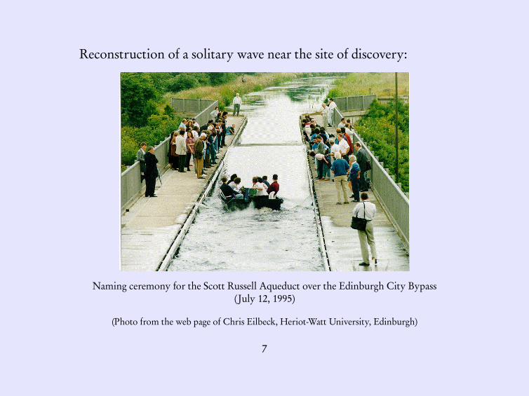
Reconstruction of a solitary wave near the site of discovery:

Naming ceremony for the Scott Russell Aqueduct over the Edinburgh City Bypass(July 12, 1995)

(Photo from the web page of Chris Eilbeck, Heriot-Watt University, Edinburgh)

7

Some results of Scott Russell’s water tank experiments:

• Solitary waves are very stable.

• The speed of a solitary wave depends on its height:

v =Æ

g (d + h)

(d = depth of undisturbed water, h =wave height)

• If one tries to generate a wave which is “too big”,it will decompose into several solitary waves, eachwith its own speed (the largest first).

• During the passage of the wave, the water particlesare displaced. (In contrast to ordinary oscillatorywaves, where they return to their original position.)

8

Scott Russell also found a wayto make canal boats go faster,with less effort for the horses:pull the boat at just the rightspeed, and it will “surf” on thesolitary wave that it generates!

But some influential scientists (Airy, Stokes) were still sceptical, sincethe solitary wave didn’t fit with their theories about water waves.

9

Water wave theory is hard!

“Now, the next waves of interest,that are easily seen by everyone andwhich are usually used as an exampleof waves in elementary courses, arewater waves. As we shall soon see,they are the worst possible example,because they are in no respects likesound and light; they have all thecomplications that waves can have.”

The Feynman Lectures on PhysicsVol. I, Sect. 51–4

10

Fluid flow basics

Velocity vector field: v(x, y, z, t )

Basic equation: the Navier–Stokes equation.

(Newton’s law applied to each “fluid particle”.)

Acceleration=Forces (pressure, viscosity, gravity)

Mass

∂ v

∂ t+ v · ∇v=−

1

ρ∇p + ν∇2v− g z

Water is (nearly) incompressible =⇒(

Constant density ρ∇ ·v= 0

11

In water wave problems, certain boundary conditionsmust hold at the free surface and at the bottom.

Major difficulty:

It is not known in advance where the surface is!

12

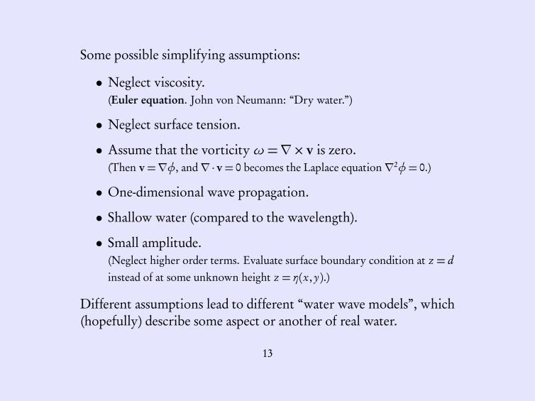
Some possible simplifying assumptions:

• Neglect viscosity.(Euler equation. John von Neumann: “Dry water.”)

• Neglect surface tension.

• Assume that the vorticityω =∇×v is zero.(Then v=∇φ, and∇ ·v= 0 becomes the Laplace equation∇2φ= 0.)

• One-dimensional wave propagation.

• Shallow water (compared to the wavelength).

• Small amplitude.(Neglect higher order terms. Evaluate surface boundary condition at z = dinstead of at some unknown height z = η(x, y).)

Different assumptions lead to different “water wave models”, which(hopefully) describe some aspect or another of real water.

13

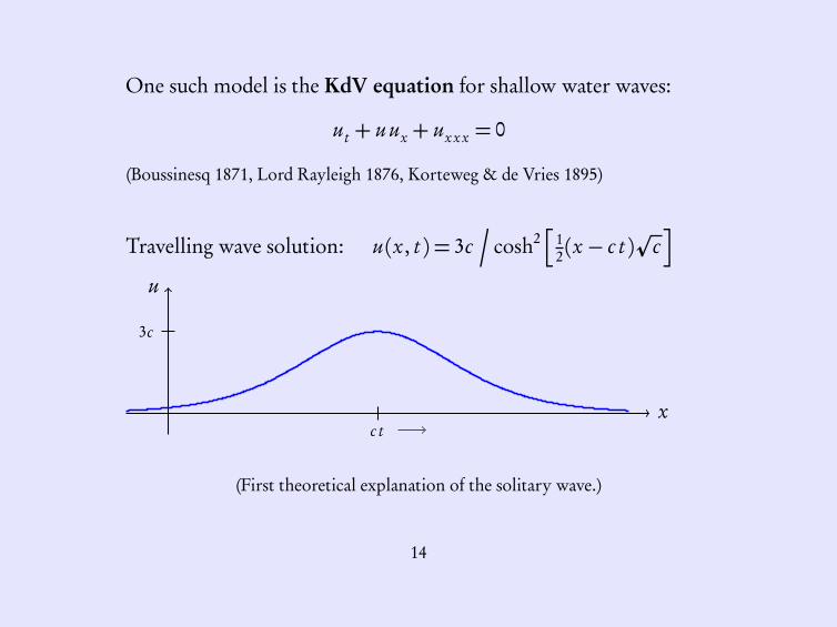
One such model is the KdV equation for shallow water waves:

ut + u ux + ux x x = 0

(Boussinesq 1871, Lord Rayleigh 1876, Korteweg & de Vries 1895)

Travelling wave solution: u(x, t ) = 3c.

cosh2h

12(x − c t )

pci

x

u

3c

c t

(First theoretical explanation of the solitary wave.)

14

Much later: surprising discoveries

Kruskal & Zabusky 1965

Numerical studies of the KdV equation.Found that several solitary waves could coexist, almostunaffected by each other: “solitons”.

Gardner, Green, Kruskal & Miura 1967

The Inverse Scattering Transform (IST), a method whichgives exact formulas for the multi-soliton solutions of theKdV equation.

(Nonlinear PDEs were considered “impossible” to solve analytically until then.)

15

Example: a two-soliton solution of the KdV equation

u(x, t ) =72�

3+ 4cosh(2x − 8t )+ cosh(4x − 64t )�

�

3cosh(x − 28t )+ cosh(3x − 36t )�2

t

x

Shown in red: u(x, 0) = 36/cosh2 x

(Cf. Scott Russell’s big wave splitting into several solitary waves.)

16

Martin Kruskal (right) playing chess against Francesco Calogero

(NEEDS ’97 conference, Kolymbari, Crete)

17

Here is a more recent shallow water wave model, derivedin 1993 by Roberto Camassa and Darryl Holm:

ut − ut x x + k ux = 2ux ux x − 3u ux + u ux x x

(u = horizontal fluid velocity, k > 0 some physical parameter)

18

They are smiling, because their paper generates lots of citations:

Previous Up Next Article

Citations

From References: 354From Reviews: 21

MR1234453 (94f:35121)35Q51 (58F07 76B15 76B25)

Camassa, Roberto(1-LANL-TD) ; Holm, Darryl D. (1-LANL-NL)An integrable shallow water equation with peaked solitons. (English summary)Phys. Rev. Lett.71 (1993),no. 11,1661–1664.

Summary: “We derive a new completely integrable dispersive shallow water equation that isbi-Hamiltonian and thus possesses an infinite number of conservation laws in involution. Theequation is obtained by using an asymptotic expansion directly in the Hamiltonian for Euler’sequations in the shallow water regime. The soliton solution for this equation has a limiting formthat has a discontinuity in the first derivative at its peak.”

c© Copyright American Mathematical Society 1994, 2010

(And this count doesn’t even include the physics literature!)

19

Why all this interest?

The Camassa–Holm equation is an integrable system.

• Lots of mathematical structure.

• IST and other methods are available.

It admits non-smooth solutions (in a suitable weak sense).

• Initially smooth solutions may lose smoothness after finite time.

• Possible model for wave breaking?

• In the limiting case k→ 0, it has peaked-shaped solitons with aparticularly straightforward structure: “peakons”.

20

The one-peakon solution

The CH equation with k = 0 can be written as

mt +mx u + 2mux = 0 m = u − ux x

Travelling wave solution: u(x, t ) = c e−|x−c t |

x

u

c

c t

21

u = e−|x| =

(

e x , x ≤ 0e−x , x ≥ 0

ux =

(

+e x , x < 0−e−x , x > 0

ux x = e−|x|− 2δ(x)

(δ is the Dirac delta at x = 0,

the distributional derivative of

the Heaviside step function)

=⇒ m = u − ux x = 2δ

22

The multi-peakon solution

x

u(x, t ) =n∑

i=1

mi (t ) e−|x−xi (t )|

xx1(t )

m1(t )

x2(t )

m2(t )

x3(t )

m3(t )

12 m(x, t ) =

n∑

i=1

mi (t )δ�

x − xi (t )�

23

This Ansatz satisfies the CH equation mt +mx u + 2mux = 0 iff

xk =n∑

i=1

mi e−|xk−xi |

mk =n∑

i=1

mk mi sgn(xk − xi ) e−|xk−xi |

(2n-dimensional dynamical system for positions xk(t ) and amplitudes mk(t ).)

Shorthand notation:

xk = u(xk) mk =−mk

ux(xk)�

(Note: Speed xk of the kth peakon = wave height at that point.)

24

The travelling wave is the case n = 1:

x1 = m1 m1 = 0

The case n = 2, with E12 = e−|x1−x2|, reads

x1 = m1+m2E12

x2 = m1E12+m2

m1 =−m1m2E12

m2 = m1m2E12

(Camassa & Holm solved this by elementary methods, using theconstants of motion M = m1+m2 and H = 1

2 m1m2E12.)

25

The Camassa–Holm peakon equations for arbitrary n were solvedusing IST by Richard Beals, David Sattinger and Jacek Szmigielski.

26

Advances in Mathematics 154, 229�257 (2000)

Multipeakons and the Classical Moment Problem

Richard Beals1

Yale University, New Haven, Connecticut 06520

David H. Sattinger2

Utah State University, Logan, Utah 84322

and

Jacek Szmigielski3

University of Saskatchewan, Saskatoon, Saskatchewan, Canada

Received May 14, 1999; accepted April 8, 1999

dedicated to gian-carlo rota

Classical results of Stieltjes are used to obtain explicit formulas for the

peakon�antipeakon solutions of the Camassa�Holm equation. The closed form

solution is expressed in terms of the orthogonal polynomials of the related classical

moment problem. It is shown that collisions occur only in peakon�antipeakon

pairs, and the details of the collisions are analyzed using results from the moment

problem. A sharp result on the steepening of the slope at the time of collision is

given. Asymptotic formulas are given, and the scattering shifts are calculated

explicitly. � 2000 Academic Press

Key Words: continued fractions; multipeakons; scattering; collisions.

1. INTRODUCTION

The Korteweg�deVries equation is a simple mathematical model for

gravity waves in water, but it fails to model such fundamental physical

phenomena as the extreme wave of Stokes [23]. The failure of weakly non-

linear dispersive equations, such as the Korteweg�deVries equation, to

model the observed breakdown of regularity in nature, is a prime motivation

in the search for alternative models for nonlinear dispersive waves [20, 24].

doi:10.1006�aima.1999.1883, available online at http:��www.idealibrary.com on

2290001-8708�00 �35.00

Copyright � 2000 by Academic PressAll rights of reproduction in any form reserved.

1 Research supported by NSF Grant DMS-9800605.2 Research supported by NSF Grant DMS-9971249.3 Research supported by the Natural Sciences and Engineering Research Council of

Canada.

27

Suppose µ is a measure on the real line such that all itsmoments βk =

∫

xk dµ(x) (k = 0,1,2, . . . ) are finite.

The Classical Moment Problem is the problem of re-covering the measure µ from its moments. (Existence?Uniqueness?)

This problem was important in the development of func-tional analysis.

Basic object: the Hilbert space L2(µ) with inner product

⟨ f , g ⟩=∫

f (x)g (x)dµ(x)

28

The moments βk determine the inner product of anytwo polynomials:*

r∑

i=0

ai x i ,s∑

j=0

b j xj

+

=r∑

i=0

s∑

j=0

ai b j

∫

x i+ j dµ(x)︸ ︷︷ ︸

βi+ j

(Important question: Are the polynomials dense in L2(µ)?)

First step: define orthogonal polynomials by doing Gram–Schmidt on the standard basis 1, x, x2, . . .

And so on. Big theory. (Very pretty, very classical, manyconnections to other parts of mathematics.)

29

What does this have to do with peakons?

To any peakon configuration (values of the xk’s and mk’s)Beals, Sattinger & Szmigielski associated a discrete string:

For k = 1,2, . . . , n, let yk = tanh xk (thus −1 < yk < 1)and gk = 2mk/(1 − y2

k). At the positions yk , put point

masses gk and connect them by weightless thread. Attachthe ends of the string to the points y =±1.

yy =−1 y =+1y = y1

g1

y = y2

g2

y = y3

g3

30

Such a string has vibrational modes (just like a guitarstring has a fundamental frequency and overtones), butonly as many as there are point masses.

The squared eigenfrequencies are denoted λ1, . . . ,λn.

One also defines numbers b1, . . . , bn which contain someinformation about the shape of the eigenfunctions.(Basically the ratio between the slopes at the endpoints.)

31

We can view this as a change of variables: from {xk , mk}to “spectral variables” {λk , bk}.

Miracle: In terms of the spectral variables, the compli-cated nonlinear CH peakon equations simply become

λk = 0 bk = bk/λk

(“Isospectral deformation” – the string’s spectrum doesn’t change!)

This system is of course easily solved:

λk = constant bk(t ) = bk(0) et/λk

32

The inverse change of variablesis given by formulas found byThomas Joannes Stieltjes in hisstudy of the moment problem.(Recherches sur les fractions continues, 1894)

This connection between the vibrat-ing string and the work of Stieltjeswas noticed by Mark GrigorievichKrein around 1950.

33

The change of variables in a nutshell (with lk = yk+1− yk):

1/2

z+

b1

z −λ1

+b2

z −λ2

+ · · ·+bn

z −λn=

=1

z ln +1

−gn +1

z ln−1+1

...+

1

−g2+1

z l1+1

−g1+1

z l0

It corresponds toconverting between two waysof representing a rational function:

LHS = partial fractionsRHS = Stieltjes continued fraction

34

Example: The Camassa–Holm three-peakon solution

x1(t ) = ln(λ1−λ2)

2(λ1−λ3)2(λ2−λ3)

2b1b2b3∑

j<k λ2jλ

2k(λ j −λk)

2b j bk

x2(t ) = ln

∑

j<k(λ j −λk)2b j bk

λ21b1+λ

22b2+λ

23b3

x3(t ) = ln(b1+ b2+ b3)

m1(t ) =

∑

j<k λ2jλ

2k(λ j −λk)

2b j bk

λ1λ2λ3

∑

j<k λ jλk(λ j −λk)2b j bk

m2(t ) =

�

λ21b1+λ

22b2+λ

23b3

�

∑

j<k(λ j −λk)2b j bk

(λ1b1+λ2b2+λ3b3)∑

j<k λ jλk(λ j −λk)2b j bk

m3(t ) =b1+ b2+ b3

λ1b1+λ2b2+λ3b3

�

λk = constant

bk(t ) = bk(0) et/λk

�

35

I have worked (mostly together with Jacek Szmigielski)on peakon solutions of some other integrable PDEs:

mt +mx u + 3mux = 0 m = u − ux x

(Antonio Degasperis & Michela Procesi, 1998)

mt +(mx u + 3mux)u = 0 m = u − ux x

(Vladimir Novikov, 2008)

Camassa–Holm, for comparison:

mt +mx u + 2mux = 0 m = u − ux x

36

The vibrational modes of a string are given by the eigen-value problem

−φ′′(y) = z g (y)φ(y)φ(−1) =φ(+1) = 0

where g (y) describes the distribution of mass.

Peakon solution of the new equations (DP & Novikov)are instead related to the third order eigenvalue problem

−φ′′′(y) = z g (y)φ(y)φ(−1) =φ′(−1) =φ(+1) = 0

which we call the cubic string.

37

The cubic string

Not selfadjoint. The eigenvalues λk are real anyway (if g is positive).(Total positivity, Gantmacher–Krein theory of oscillatory kernels.)

Inverse spectral problem for discrete case gives explicit formulas forthe peakon solutions.(Quite a lot harder than for the ordinary string.)

Instead of orthogonal polynomials: Cauchy biorthogonal polynomals

⟨ f , g ⟩=∫∫ f (x) g (y)

x + ydα(x)dβ(y)

¬

pi , q j

¶

=

(

1, i = j0, i 6= j

(Bertola–Gekhtman–Szmigielski, 2009, 2010)

38

Example: The Degasperis–Procesi three-peakon solution

x1(t ) = lnU3

V2x2(t ) = ln

U2

V1x3(t ) = ln U1

m1(t ) =U3(V2)

2

V3W2m2(t ) =

(U2)2(V1)

2

W2W1m3(t ) =

(U1)2

W1

whereU1 = b1+ b2+ b3 V1 = λ1b1+λ2b2+λ3b3

U2 =(λ1−λ2)

2

λ1+λ2b1b2+

(λ1−λ3)2

λ1+λ3b1b3+

(λ2−λ3)2

λ2+λ3b2b3

V2 =(λ1−λ2)

2

λ1+λ2λ1λ2b1b2+

(λ1−λ3)2

λ1+λ3λ1λ3b1b3+

(λ2−λ3)2

λ2+λ3λ2λ3b2b3

U3 =(λ1−λ2)

2(λ1−λ3)2(λ2−λ3)

2

(λ1+λ2)(λ1+λ3)(λ2+λ3)b1b2b3 V3 = λ1λ2λ3U3

W1 =U1V1−U2 = λ1b 21 +λ2b 2

2 +λ3b 23 +

4λ1λ2

λ1+λ2b1b2+

4λ1λ3

λ1+λ3b1b3+

4λ2λ3

λ2+λ3b2b3

W2 =U2V2−U3V1 =(λ1−λ2)

4

(λ1+λ2)2λ1λ2(b1b2)

2+ · · ·+4λ1λ2λ3(λ1−λ2)

2(λ1−λ3)2b 2

1 b2b3

(λ1+λ2)(λ1+λ3)(λ2+λ3)+ . . .

39

Now, finally, some combinatorics!

Lindström’s Lemma

If X is the path matrix of a planar network,then the minor (=subdeterminant) taken fromrows i1, . . . , ik and columns j1, . . . , jk equals thesum of the weights of the non-intersecting pathfamilies from the source nodes i1, . . . , ik to thesink nodes j1, . . . , jk .

(Karlin & McGregor 1959, Lindström 1973, Gessel & Viennot 1985)

40

Example:

1

2

1

2

a

b

c

d

e

f

gPath matrix:

X =�

ae + ad f ad gb e + b d f + c f b d g + c g

�

detX = ae · c gAll other terms cancel in pairs.(“Switch paths at first intersection”is a sign-reversing involution.)

1

2

1

2

a

b

c

d

e

f

g

+ad f · b d g

−ad g · b d f

41

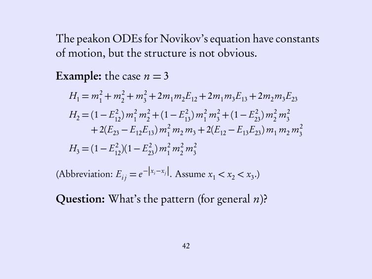
The peakon ODEs for Novikov’s equation have constantsof motion, but the structure is not obvious.

Example: the case n = 3

H1 = m21 +m2

2 +m23 + 2m1m2E12+ 2m1m3E13+ 2m2m3E23

H2 = (1− E212)m

21 m2

2 +(1− E213)m

21 m2

3 +(1− E223)m

22 m2

3

+ 2(E23− E12E13)m21 m2 m3+ 2(E12− E13E23)m1 m2 m2

3

H3 = (1− E212)(1− E2

23)m21 m2

2 m23

(Abbreviation: Ei j = e−|xi−x j |. Assume x1 < x2 < x3.)

Question: What’s the pattern (for general n)?

42

Conjecture early on in our investigations:

Hk = sum of all k × k minors (subdeterminants ) of

the n× n matrix X with entries Xi j = mi m j Ei j

X =

m21 m1m2E12 m1m3E13

m1m2E12 m22 m2m3E23

m1m3E13 m2m3E23 m23

1 1

2 2

3 3

m1 m1

m2 m2

m3 m3

E12

E23

E12

E231− E2

12

1− E223

43

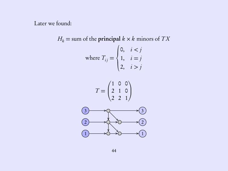
Later we found:

Hk = sum of the principal k × k minors of T X

where Ti j =

0, i < j1, i = j2, i > j

T =

1 0 02 1 02 2 1

1 1

2 2

3 3

44

Does this result agree with the conjecture? Yes, and there is nothingspecial with our particular matrix X , except that it is symmetric.

The Canada Day Theorem

For any symmetric n × n matrix X , the sumof all k × k minors of X equals the sum of theprincipal k × k minors of T X .

Example: n = 2 (Too simple, really. For n ≥ 4 it starts to get more interesting.)

X =�

a bb c

�

T X =�

1 02 1

��

a bb c

�

=�

a b2a+ b 2b + c

�

k = 1: a+ b + b + c = a+(2b + c)k = 2: detX = det(T X ) (true since detT = 1)

45

Like as the waves make towards the pebbled shore,So do our minutes hasten to their end

William Shakespeare, Sonnet LX