From Two-Way to Multi-Way: A Comparative Study for Map-Reduce Join Algorithms

MARWA HUSSIEN MOHAMED

Information System Arab Academy For science And Technology and maritime transport

CAIRO, EGYPT Eng_maroo1@yahoo.com

MOHAMED HELMY KHAFAGY

Computer Science Fayoum University CAIRO, EGYPT

Mhk00@fayoum.edu.eg Abstract: - Map-Reduce are a programming model which is widely used to extract valuable information from enormous volumes of data. Map-reduce designed to support heterogeneous datasets. Apache Hadoop map-reduce used extensively to uncover hidden pattern like, data mining, SQL, etc. The most important operation for data analysis is joining operation. But, map-reduce framework doesn’t directly support join algorithm. This paper explain and compare two- way and multi- way map-reduce join algorithms for map reduce also we implement MR join Algorithms and show the performance of each phase in MR join Algorithms. Our experimental results show that map side join and map merge join in two-way join algorithms has longest time according to preprocessing step sorting data and reduce side cascade join has the longest time at Multi-Way join algorithms.

Key-Words: - Hadoop, Map-Reduce, Multi-Way Join, Two-Way Join, Ubuntu

1 Introduction Map-Reduce [1, 2] at academic or business area are widely used for vast amount data analysis. It uses commodity of considerable number hardware to process large scale of data in a reasonable time. It’s less cost for mining valuable hidden information in this significant data compared to previous techniques. The major benefits of map-Reduce are an easiest framework to analysis data across shared nothing clusters and handling fault tolerance.

Cloud computing and data-intensive analysis [3] are applications do massive operations with processing millions of records and produce rarely updates with analytic systems. Parallel DBMS, Map-Reduce (MR) paradigm, and columnar storage these techniques had multiple data sets and used to analysis large scale data [3]. All previous algorithms Needs to perform various join operation due to large scale of data and needed to get more valuable information after joining.

The Apache Hadoop [4] it's using simple programming models to handle and distribute huge data sets via computer clusters. It's can handle thousands of machine, it's can detect and handle failure can happened between application layers to support fault tolerance.

Unfortunately, high-level language Pig [3] is a framework for analyzing large unstructured and semi-structured data on top of Hadoop and Pig Latin is declarative language used like SQL and it's the high level language interface for Hadoop. Hive query language is the primary data processing method for cloud data platform which is powered by Apache Hive. Hive query language can support users to handle, manage and store data on cloud.

Hive query language using Hadoop map reduce to accept queries from users. So that high-level language Pig, Pig Latin and Hive QL [3] are methods to solve joined algorithm problem that is not supported in Map-Reduce.

This paper compare some existing types of Two-way and multi-way join algorithms that's used map side join and reduce side join. Algorithms we will discuss in Two-way join are map side join, In

WSEAS TRANSACTIONS on COMMUNICATIONS Marwa Hussien Mohamed, Mohamed Helmy Khafagy

E-ISSN: 2224-2864 129 Volume 17, 2018

memory join, Broadcast join, Map merge join ,Memory backed join ,Reduce side join , Repartition join and bloom filter join all this algorithms are used only one phase to do join operation. Some types of two-way join algorithms has more than one phase to do join operation like semi-join, per split semi-join and map reduce merge join. Multi-way join algorithms are Map Side join, Reduce Side one shot join and reduce side cascade join. All this algorithms we do experimental results on various data size and running data using TPC benchmark to show algorithms performance.

The rest of this paper is organized as follow: Section 2 describe map-reduce architecture and covers Hadoop, section 3 describe various types of two-way and multi-way map-reduce join algorithms and list some of advantage and disadvantage of these algorithms, Section 4 describe comparative analysis of join algorithms, Section 5 show our experimental results while increasing in data size and finally section 6 conclusion and future work.

2. Map-reduce and Hadoop

Map-reduce are [1] a programming model popularized by Google since 2004. It’s used with large-scale datasets and processing data on a shared-nothing cluster.

Hadoop Apache Hadoop [4] is an open source, and it's used new ways to store and process big data. 2.1 Map-reduce framework Map-Reduce accomplish high performance by partitioning the processing into small units of work that can run in parallel across thousand of nodes in the cluster. Users only need to write the function without thinking of parallel and distributed processing [2, 4].

Applications like graph analysis, text analysis, Indexing and Search, etc… are difficult to implement by standard SQL. Arising of map-reduce solve this problem by processing and analyzing an enormous number of multi-structured data. Map-Reduce have a high scalability and fault tolerance by data partitioning and replication [5] and load balancing [2, 6 and 7].

The programming model is consisting of the following:

1. Do some iteration on the input. 2. Generate a key / value pair from the input.

3. Using the key of every input became easiest to group all intermediate values.

4. Make iteration based on resulting groups. 5. Do Reduction on each group to generate

output. Map-Reduce[4] user computation focus mainly on two important functions Map and Reduce figure 1 shows the operation of Map-Reduce and figure 2 show the Map-Reduce execution overview . Fig.1 Operation of map-reduce

Implementation of map-reduce 1 Map-reduce has one master node sends job to

all task tracker by divide the input file into M splits by using the key value pair and following task tracker jobs by using heart beat to avoided failed.

2 Task Tracker writes their output to a local disk and partition this output result to some reduce tasks.

3 Job Tracker assign reduce tasks to task tracker Then reduce workers read the new key/value input data from local disk then produce final output result after sort and aggregate data by using the key.

4 If one task tracker fails job tracker assign node task to another one workers.

2.2 Hadoop Hadoop Map-Reduce [4] is an open source implementation by Apache. Hadoop Distributed File System (HDFS) used to distribute data across machines in the network. It has two separate servers one to store file system metadata (name-node) and the second to store application data (data node).

Name node run on a single master machine, and it has all information about other machines in the

Step 1: the MAP Phase User provides the MAP function

• Input: (key, value) • Output: (key, value) System applies

the map function in parallel to all (input key, value) pairs in the input file.

Map: (k1: v1) [(k2:v2)] Step 2: the REDUCE Phase

User provides the REDUCE function: • Input: (Intermediate key, bag of

values) • Output: all pairs with the same key

are grouped together and sent values to the same reducer to get the output result.

Reduce: (k2: [v2]) [(k3: v3)]

WSEAS TRANSACTIONS on COMMUNICATIONS Marwa Hussien Mohamed, Mohamed Helmy Khafagy

E-ISSN: 2224-2864 130 Volume 17, 2018

cluster. Data node processes run on all other machines and communicate with name node to obtain data on their local drive and works like workers. Figure 3 shows map task and reduce task at Hadoop.

The Map-Reduce framework of Hadoop [8] consists of single Job Tracker and a number of Task Tracker process The Job Tracker usually runs on the same master machine as the Name node. Task Tracker runs at the data node.

Fig. 2 An execution overview of map-reduce based on [4].

Fig. 3 Shows map task and reduce task at Hadoop-based on [8].

3 Map-Reduce Join Algorithms Map Reduce is a programming model build to support heterogeneous data for analyzing and finding hidden pattern, but isn’t support join algorithms directly as in[4,8]. We will discuss different joining two-way and multi-way datasets algorithms using map-reduce

Basic methods for processing joins in Map-Reduce include: I. Distributing the smallest operand(s) to all nodes, and performing the join by the Map or Reduce function. 2. Map-side join and reduce-side join.

3.1 Two-way join algorithms Two-way join algorithms are used to join two dataset R and L as in equation 1. R (A, B) ⋈ L (B, C) (1)

In this section we will cover two-way join algorithms using map function only to do join operation like map side join, In Memory join, broadcast join, memory backed join and map merge join. Other types of two-way join using map function and reduce function like reduce side join, repartition join and bloom filter join. Finally two-way join using more than one phase and used map function and reduce function are semi-join and per split semi-join. 3.1.1 Map side join Map side join is a natural way of join algorithms for datasets that perform join by using the map function only and isn’t any needs for reduce function. Map side join framework [3,4] is more helpful to be used when the size of one dataset is relatively too small to fit in memory. It uses the Hadoop framework to do a pre map phase that used memory hash table to read data from HDFS and splitting each table data into the same number of partition then sort each table by using the join key. Mappers must group all records with the same key in the same partition finally at map phase for each partition scan the data and join based on key/value pairs and output the result. We used the abbreviation MSJ for this algorithm and Figure 4 Illustrate data flow for map-Side Join Advantages:

1. Map side join are more efficient for minimizing the cost because we are avoid using shuffling and reduce phases.

Disadvantage: 1. Every dataset must be sorted and

partitioned under condition of the join key. 2. Map side join can’t be used on the tables

which contain huge data in both of them. 3. There is a problem when the smaller set

can’t be fit into memory.

DFS

Input data

Reduce& Output

Merge

Sort and Shuffle

Map

WSEAS TRANSACTIONS on COMMUNICATIONS Marwa Hussien Mohamed, Mohamed Helmy Khafagy

E-ISSN: 2224-2864 131 Volume 17, 2018

Fig.4 Data Flow for Map-Side Join based on [4]. 3.1.2 In-memory Join It’s an improved join type of map side join it used when one of the two datasets are small enough to be fit in memory as described in [3]. It has some restriction that the small dataset must be completely fit in memory. It uses hash tables to broadcast the small dataset to every mapper and save a copy in memory. it uses a lookup hash table to find matches values between the two data sets from the other input data. Algorithm keeps away from moving and sorting input and output data for two relations. We used the abbreviation IMJ for this algorithm Figure 5 shows pseudo code for in memory join [3] Advantage:

1. Resistance to data skew.

2. We are reading part of the second dataset according to the join condition

Disadvantage:

1. Smaller data must be completely fitted in memory

Fig. 5 shows pseudo code for in memory joins [3] 3.1.3 Broadcast join Broadcast join algorithm[3,4] are the same as in memory join but small data set must fit in the memory but not completely it's called hash join because it's used hash table .load one dataset into memory, stream over other dataset. We used BJ abbreviation for this algorithm. Figure 6 show pseudo-code for broadcast Join [9] Broadcast join implementation:

1. if R fits into memory and R << S

2. Distribute R to all nodes 3. Map over S, loads R in memory for each

mapper and hashed by join key 4. look up join key in R For every tuple in S, 5. There are no reducers, unless for

regrouping or resorting tuples. Advantage:

1. Decrease I/O time by avoiding shuffling data

2. Decrease I/O cost by avoiding using reduce phase.

Disadvantage: 1. Sensitive to data skew 2. When the size of table more than memory

size can cause memory overflow.

3.1.4 Map merge join Map merge join algorithms adding a new merge function to the map side join algorithms also reduce phased are not used by this join algorithm[2]. Mappers get two data sets and partition the data sets equally on constraint of join key and sorting data sets. Mappers read the input key/value pair and merge them, then emit resulting Tuples. It works similarly to sort-merge join in DBMS[8] and we used the abbreviation MMJ .

Advantage: 1. We aren’t forced to read other data set

completely it being on demand 2. Memory overflow can be avoided Disadvantage: 1. We need to sort two datasets 2. Sensitive to data skew

3.1.5 Memory backed join Memory backed join[4] it works similar to broadcast join that fit the small relation completely in memory of each node of the cluster with some different . It used when one of the two data sets is can’t be fit into memory. We decide the partition size of the node memory and partition data according to this node size. Smaller data sets can be read from distributed cache or a distributed file system. Mappers can iterate over the data sets according to data partition numbers. A Memcached open source system is used to store datasets into memory of many machines by distributed key-value and perform join if join key matches. We used the abbreviation MBJ. Advantage: 1. Mappers at each node read the same number of

tuples sequentially so that this algorithm has a resistance to data skew.

WSEAS TRANSACTIONS on COMMUNICATIONS Marwa Hussien Mohamed, Mohamed Helmy Khafagy

E-ISSN: 2224-2864 132 Volume 17, 2018

Disadvantage: 1. One of the two data sets size must be

completely fit the memory or divide the data size according to memory size.

Fig. 6 Show pseudo-code for broadcast joins [9]. 3.1.6 Reduce side join

Reduce side join has no limitation on the size of your datasets, it can join many data sets together at once as you need and used to join multiple large datasets are being joined by a foreign key[11].

Map function prepares join operation to emit the join key as intermediate key/value , and map over both data sets to tag every record with a table name and outputs a list of tagged key/ value pair to know where the record come from. Hash partitioned function is used to partition, sort and merge the output (intermediate key/value) of the map function and distributes all to reduces.

All records with the same join key and different tag are fit to the same reducer and perform cross product to these records to join results. Figure 7 shows a full map phase for reduce side join [8] Figure 8 shows complete reduce phase of a reduce side join [8] Figure 9 shows data flow example for reduce side join figure 10 pseudo code for reduce side join [3] we used the abbreviation RSJ for this algorithm. Advantage: 1. Easiest to implement. 2. Reduce side join can use any datasets size with

no limitation. 3. Reduce side join has a most time-consuming

because it contains an additional phase to transmit the data from one phase to another phase over the network.

Disadvantage: 1. Reduce-Side join approach may cause a

network bottleneck due to shuffling of both datasets over the network.

2. Sensitivity to the data skew.

Fig. 7 Full map tasks for reduce side join [8].

Fig. 8 Shows complete reduce phase of a reduce side join [9]

Fig. 9 Data flow Example for Reduce side join

WSEAS TRANSACTIONS on COMMUNICATIONS Marwa Hussien Mohamed, Mohamed Helmy Khafagy

E-ISSN: 2224-2864 133 Volume 17, 2018

3.1.7 Repartition joins

Repartition join is a type of reduce side join that works by adding a tag to the input key and to value to determine any table where record. It partition records according to join key and group all records together before reduce phase. At the shuffling phase, all records with the same join key are fitted same reducer.

It solves the buffering problem for all records during the join process. Figure 11 show pseudo-code for repartition join [10].We used the abbreviation RJ for this algorithm. Algorithm steps:

1. Uses composite Keys: tag+ key 2. Where tag is an identifier for the parent table 3. (key, value) = (tag + key, value) 4. Partition phase hashes the key part of the

compound key 5. Guarantees tuples with same join key are sent

to the same reducer 6. Intermediate data is sorted only by key part 7. We load the smaller relation into memory by

using the tag portion of compound key and perform the join

Improved repartitions join: Map function tags the table key not the record tag then output composite join key / table tag as in [10]. This impact on performance and reduce network load

Fig. 10 pseudo code for reduce side join[3] Advantage: 1. Solved large data sets size that extended than

memory size by partitioning data. 2. Resistance to data skew Disadvantage: 1. All records in the large table may be buffered. 2. The key cardinality is small. 3. Adding a tag to record and value can cause

network bottleneck and overhead on network load.

Fig. 11. show pseudo-code for repartition joins [10]

3.1.8 Semi -join

Often, used when the size of one data sets is extremely larger than the other. Multiple records will not be used for join so that deleting these usefulness records will affect the network workload and size of datasets to join .we used SJ as abbreviation for this algorithm.

The semi-join framework has three phases: Firstly, works a whole map-reduce job that in the

map function using a hash table to determine a set of unique join key from second table whose join key are foreign key and do map function to get all join key and use reduce function to eliminate redundant records and output one file has join key .

Secondly, map phase load output file from phase one into memory and load the second table into HDFS and do map function to get key value pair to compare with the output table from first phase and get all key records can do join with this result and output second file from this phase.

Finally, we have output files from the second phase with join key records and load first table in memory and do join using broadcast join as discussed earlier. Figure 12 show pseudo-code for semi-join [10]. Semi join requires 3 Map-Reduce jobs:

1. Get a list of unique join keys, S.uk (Map + Reduce)

2. Load S.uk into memory and loop through R. If a record’s key is found in S.uk, emit it. Now we have a list of records in R to be joined.

3. Use a broadcast join to perform the join with S

WSEAS TRANSACTIONS on COMMUNICATIONS Marwa Hussien Mohamed, Mohamed Helmy Khafagy

E-ISSN: 2224-2864 134 Volume 17, 2018

Fig. 12. Show pseudo-code for semi-join [10] Advantage:

1. Get high performance at large tables data. 2. Increase the performance by deleting

usefulness data. Disadvantage:

1. Extra scan for the large table that affects the I/O costs.

2. Takes more time than previous algorithms with small size of data.

3.1.9 Per-split semi-join

Per split semi-join[10] solve the problem with semi-join that we send all filtered records to every split of second table that's will not matched join key so that per-split semi-join partition first table join key as number of partition without using reduce function with the first phase .we used PSJ as abbreviation for this algorithm. Consist of three separately map-reduce phase: 1. Map phase generates the set of unique (different,

individual) join keys in a split Mi of M and stores them in the Distributed file system [12,13,14] Mi.uk

2. Map function distributes all N records in memory hash table to read unique join key may join with Mi.uk files.

3. Each corresponding record is outputted with a tag NLi , which is used by the reduce function to collect all the records in N that will join with Mi Files with tag NLi join with Mi files with direct join.

Advantage: 1. Get high performance at large tables data. 2. Increase the performance by using deleting 3. Move only records from the large dataset that

will join with small one. Disadvantage: 1. Second phase are highly cost. 2. Takes more time than previous algorithms with

small size of data.

3.1.10 Bloom filter join

Bloom filter is used to filter out redundant records from one of the two data sets at the map phase [15] by constructing bloom filters at the map phase as in [16]. Difficult to apply bloom filter because input data at map-reduce has no processing order its schedules map reduce tasks only not the input splits and bloom filter need to be distributed to all nodes in the cluster.

Bloom filter are used to reduce the number of candidate pairs to consider the similarity. Figure 13 show pseudo-code for bloom filter join [3] Figure 14 show bloom filter data flow [16]. We used BFJ as abbreviation for this algorithm.

Hadoop algorithm modified to apply bloom filter: 1. Input dataset at map phase is processed

sequentially for joins. 2. Input data set processing order effect on the

processing cost. 3. Bloom filter execution flow is build dynamically

within a single map-reduce job. Blooms filter execution overflow: 1. Job submission: for every table a map task and

reduce task are created by job tracker and distribute tasks on task tracker (m1 map task for table r and m2 map task for s and reduce tasks)

2. First map phase: first map task tracker read the input split for the tasks and produces key value pair output Local filter construction: every key-value pair generated.

3. Map tasks are divided into r partitions and sent to task tracker. At each key partition bloom filter are constructed.

4. Global filter merging: when m1 map tasks are completed job tracker send to all task trackers to send their local filter resulted to job tracker. Then job tracker construct global filter to dataset R. when job tracker finishes their tasks new map phase to the other data sets is build.

5. Second map phase: we repeat the first map phase steps again for the other data sets till job tracker end the process then reduce phase to the two data sets are constructed

6. 6)Reduce phase: it gets two map phases output like reduce phase at Hadoop and then sorts the intermediate pairs then run reduce function to produce output in the last output path.

Advantage: 1. Map tasks are assigned in order of the data sets. 2. Bloom filter are constructed in a distributed

fashion. 3. Bloom filter Increased join performance. 4. Number of map tasks and reduce tasks used are

decreased by using bloom filter to join operation. 5. While the intermediate records are reduced reduce

phase are completed first.

WSEAS TRANSACTIONS on COMMUNICATIONS Marwa Hussien Mohamed, Mohamed Helmy Khafagy

E-ISSN: 2224-2864 135 Volume 17, 2018

Fig.13. Show pseudo-code for bloom filter joins [3] Disadvantage:

1. Performance of join algorithm depends on the bloom filter size.

2. Data sets with large size can effect on bloom filter performance.

3. Bloom filter isn’t filter out tuples before join so it may cause redundant.

4. While global filter for the first map phase still working we can’t start another map function so that is may increase in time.

5. If the number of intermediate results has significant execution time is increased compared to Hadoop.

Fig.14. bloom filter data flow [14]

3.1.11 Map-Reduce Merge Join

Map-reduce merge join[17] used with massive datasets (heterogeneous datasets) it has two completely map-reduce phases and one merge phase that select the data from reduce phase output result according to join condition . At merge phase, we have two types of join algorithms we can use a hash join or sort merge join. Figure 15 show overview of map-reduce merge

Signature of map-reduce merge are given below: 1. Map phase: input (k1, v1) → list of intermediate

[(K2, v2)]. 2. Reduce phase: aggregates list (K2, [v2]) →output

another list (K2, [v3]). 3. Merge phase: combine the two reduce outputs

((K2, [v3]), (k3, [v4])) → output new join result (k4, [v5])

Fig.15 Overview of Map-Reduce Merge based on [17]. Map Reduce merge join algorithm works by a map phase and reduce phase independently on the two data sets, merge phase takes two reduce phases output according to the join condition. Internally operation inside merge phase[18]: 1. Partition Selector is selector that determines which

data partitions produced by up-stream reducers should be retrieved and then merged.

2. Configurable iterators – it can implement two different join algorithms by two logical operators it includes sort-merge join and nested loop join

3. Processor – used to handle processing data from different datasets

4. Merger – used to apply merger function for processing data from two sources. Figure 16 show data flow for map reduce module merge [18].

Advantage: 1. It can be used with heterogeneous data sets. 2. It used efficiently with two-way join and can be

used with multi-way join. 3. Using a sort merge join is efficient than nested

loop join when using equal join.

WSEAS TRANSACTIONS on COMMUNICATIONS Marwa Hussien Mohamed, Mohamed Helmy Khafagy

E-ISSN: 2224-2864 136 Volume 17, 2018

4. Using nested loop join with complicated joins increases the complexity to understand the execution flow of a job.

5. It increases flexibility and usability. Disadvantage:

1. Adding new merge phases that increase the I/O cost.

2. Increase in complexity for data flow.

Fig.16 data flow for map reduce module merge based on [18].

3.2 Multi-way joins algorithms

Multi-way join usually used to join more than two data sets like R and S and T tables [19] as in equation 2.

R (A, B) ⋈ L (B, C) ⋈ T (C,D) (2)

In this section we will cover the following multi-way join algorithms map side join, reduce side on shot join and reduce side cascade join and explain advantage and disadvantage of every algorithm.

3.2.1 Map-Side Join

It works like to two-way map side join algorithms it handles many data sets according to some constraints as in [11] .All datasets must use same comparator and sort according to them. Only one practitioner must be used to partition all the datasets. A key used with each data sets are used in the same partition and this key must be identical. Advantages: 1. Map side join are more efficient for minimizing

the cost because we are avoid using shuffling and reduce phases.

Disadvantage: 1. Every dataset must be sorted and partitioned under

condition of the join key. 3.2.2 Reduce-Side One-Shot Join

Reduce side algorithm uses a function from reduce side join from two-way join which uses tags value for every record to know the record and datasets [11, 20]. It passes Tables Tags for every table need to be joined to know how many tables mapper and reduces the work with it. Figure 17 shows data flow for reduces side one shot join. It has three phases listed as following: 1. Map phase: Mapper reads data from the input data

splits and tags each tuple with the table tag based on the datasets they originate from.

2. Partitioning and Grouping Phase: it is ignoring the tag value and partition and group data according to the key only.

3. Reduce phase: The reduce phase gets the tuples sorted according to key, tag. All tuples have the same join key values are going to the same reducer. Every join key has a single reducer function. Buffers are created by the reducer to hold all the datasets without the last one. Then output joined tuples have written.

Advantages: 1. No needs for a preprocessing phase. 2. No intermediate results. Disadvantage: 1. Some memory problems from buffering tuples in

reduce side. 2. Sensitive to data skew

3.2.3 Reduce-Side Cascade Join

Reduce-Side Cascade Join [11] is the exact same as reduce side join of two data sets and it’s an iterative function to reduce side join. It uses calling program to create multiple join datasets only two datasets at the same time. Considering if we have four datasets (t1, t2, t3, t4) we join t1 with t2 result t5 then join t3 with t4 result t6 finally join t5 with t6 this is the final output. Advantages 1. Best for I/O cost and needed for buffering records

rarely. 2. Can join any number of datasets. Disadvantages 1. Multiple jobs in the cluster need to set up that

cases non-trivial overhead. 2. many memory spaces are taken by intermediate

results

Data 1 Data 2

Data 3

Partition selector

Left processor Right processor

Left Iterators Right Iterators

Merger

WSEAS TRANSACTIONS on COMMUNICATIONS Marwa Hussien Mohamed, Mohamed Helmy Khafagy

E-ISSN: 2224-2864 137 Volume 17, 2018

3.2.4 Comparison for Multiway joins

According to our previous illustration to multi-way join algorithm we can decide which type of algorithms may be preferable according to our data size we need to join [11]. When we have the same number of tuples and same key space Reduce-Side One-Shot Join algorithm performance are nearly to the map side join algorithms.

Reduce side one shot are failed and memory overflow when increasing the size of datasets over than the total memory size .reduce side cascade join is the best join algorithms when increasing data sets size than memory size and when reduce side one shot join has memory overflow.

4 Comparative Analysis of Join

Algorithms The join algorithm features are presented in table 1. Range practitioner used to solve approaches that are sensitive to data skew [3]. Algorithms without tagging have not additional workload on memory for transferring extra data through the network [3], and it’s more preferable. Map-reduce join algorithms performance is improved in case of semi-join data low selectivity [10] and memory overflow possibilities are reduced.

According to table 1 most of the join algorithms are sensitive to data skew except in memory join and memory backed join. Join Algorithms using map side join are preferable than reduce side join according to shuffling and sorting phases and network overload. Preprocessing steps before map side phases are affected in performance .using bloom filter algorithms affect in performance and avoid memory overflow. If one of the two data sets is small enough to fit in memory we preferable to use map side join.

Fig. 17 Data flow for Reduce side one shot join based on [11].

TABLE 1: JOIN ALGORITHMS FEATURES

Two-way join

algorithm

Pre-processi

ng

number of

phases

Need distr. cach

e

Memory overflow

Join algorithm

Map-side join yes one no yes Hash join

Broadcast join no one yes

Size of smaller

dataset is large

Hash join

Reduce side join

Yes for one of the two datasets

two no

Tuples with the same key

have large size

Cross product

Map merge join

Yes for two

datasets one no no Sort Merge

join

Memory backed

join no one no

Size of the

Smaller dataset is large than memory

size

Hash join

Repartition join

Yes for one

of the two

datasets

two no

Number tuples for the same

key is large

Sort Merge join

Semi -join yes three yes

Size of filtered datasets is large

Hash join

Per-split semi-join yes three yes

Size of filtered datasets is large

Hash join

Bloom filter join no two yes

Size of data large

than bloom filter

Hash join

Map-Reduce merge join

no three yes

Size of the two datasets is very large

Nested loop join and sort

merge join

5 Experimental Results We present experimental results of our implementation. We have 3 cluster machines one of them master node (name node) and two other are slave node (data node). Cluster configuration consists of Intel core i5 2.4 GHz processor, 4 GB memory for every node, 500 GB SATA disk and operating system Ubuntu 20.203.0 Linux with Apache Hadoop release 1.2.1.

5.1 Dataset We use TPC-H benchmark [21] dataset to evaluate our implementation with original Hadoop. We use two table customers and orders to join according to join key where O_CUSTKEY= C_CUSTKEY where customer table has 500,000 record and table orders has

WSEAS TRANSACTIONS on COMMUNICATIONS Marwa Hussien Mohamed, Mohamed Helmy Khafagy

E-ISSN: 2224-2864 138 Volume 17, 2018

1,500,000 records as the start size for our experiment and increasing number of records for two tables as shown in table 2 .

Table 2: Number of Records in Tables

Number of records Order table Customer table 2 million 1,500,000 500,000 4 million 2,500,000 1,500,000 6 million 4,000,000 2,000,000 10 million 6,000,000 4,000,000 12 million 8,000,000 4,000,000

5.2 Two-Way Join Experimental Result

We present the execution time performance for every phase of join at map-reduce like sort, map, shuffle, reduce phases time Figure 18 has different graphs show Two Way Join algorithms Result-performance while increasing in data size.

our experiment result show that map side join and map merge join has the worst time compared with the other join algorithms to complete join according to preprocessing phase sorting data running time for this two algorithms are increasing in time by 40% from 10 million records to 12 million records .

Reduce side join and repartition side join using two phases shuffle and reduce phase that's increase in cost but reduce in running time compare to map side join and map merge join. Repartition join used join key to repartition data and using table tag to complete join phase this step takes long time than reduce side join at 10 million records to 12 million records reduce side join increased in time by 19% and 48% for repartition join.

Bloom filter join has reduced data shuffling problem that takes time as in repartition join and reduce side join by constructing bloom filter as preprocessing step and eliminating unused record to join from the second table at map phase while running data from 10 million record to 12 million records time increased by 18 % .

In memory join and broadcast join and memory backed join has the best time performance because it's using hash table and distributed cache to do join and isn't needed to use sorting or shuffling or reducing phases that increase in cost bust when data size increased than memory size cause memory overflow

Figure 18 (F) show the total time for each algorithm at different size of data and table 3 has a total time for each join algorithms with different data size that show change in running time.

Algorithms of two-way join with more than one phase chart figure 19 show total join time because semi-join and presplit semi-join has different three map-reduce phases. Semi join and per-split semi-join algorithms are highly cost with small data sets but while increasing in data size do the best performance time than two-way join algorithms discussed earlier according to extra scan for large table and figure 18 show that semi-join running time better than presplit

semi-join according to very highly cost for the second phase and extra scan for large table running time from 10 million records to 12 million records increased by 2% for semi-join and 9% for presplit semi-join. Table 3: Total time for all join algorithms

Join algorithm 2 million

4 million

6 million

10 million

12 million

In memory Join (IMJ) 30 43 44 48 61

Broadcast Join ( BJ) 31 46 48 51 64

MemoryBacked Join( MBJ) 32 48 49 52 66

bloomfilter Join ( BFJ) 45 59 90 108 128

ReduceSide Join (RSJ) 54 71 109 130 155

Repartition Join (RJ) 87 101 133 143 212

Map Side Join (MSJ) 162 198 245 268 378

MapMerge Join ( MMJ) 164 203 250 275 387

Semi Join (SJ) 140 143 146 150 160

Per -Split Semi Join (PSJ)

160 164 168 170 175

Fig.18-a. 2 million records

Fig.18-b. 4 million records

WSEAS TRANSACTIONS on COMMUNICATIONS Marwa Hussien Mohamed, Mohamed Helmy Khafagy

E-ISSN: 2224-2864 139 Volume 17, 2018

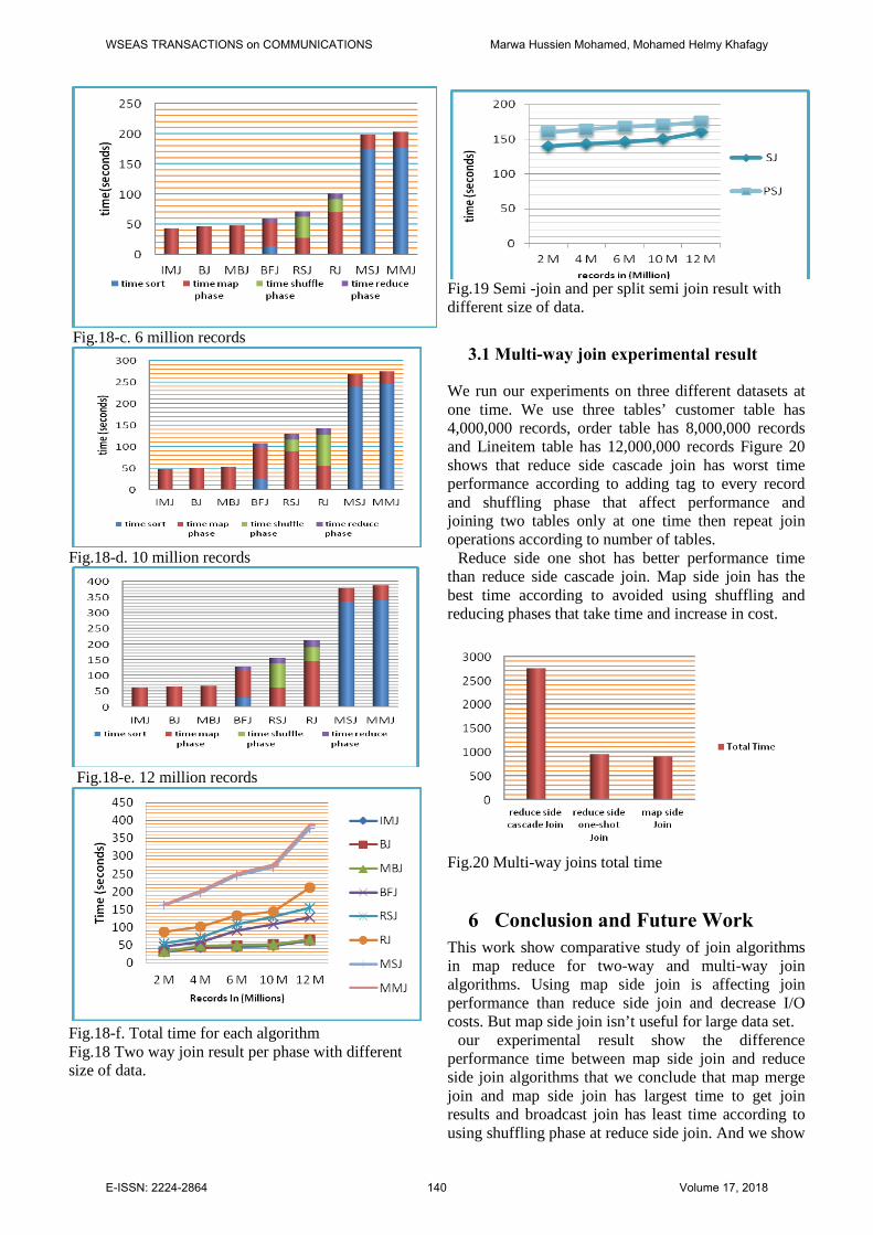
Fig.18-c. 6 million records

Fig.18-d. 10 million records

Fig.18-e. 12 million records

Fig.18-f. Total time for each algorithm Fig.18 Two way join result per phase with different size of data.

Fig.19 Semi -join and per split semi join result with different size of data.

3.1 Multi-way join experimental result

We run our experiments on three different datasets at one time. We use three tables’ customer table has 4,000,000 records, order table has 8,000,000 records and Lineitem table has 12,000,000 records Figure 20 shows that reduce side cascade join has worst time performance according to adding tag to every record and shuffling phase that affect performance and joining two tables only at one time then repeat join operations according to number of tables.

Reduce side one shot has better performance time than reduce side cascade join. Map side join has the best time according to avoided using shuffling and reducing phases that take time and increase in cost.

Fig.20 Multi-way joins total time

6 Conclusion and Future Work

This work show comparative study of join algorithms in map reduce for two-way and multi-way join algorithms. Using map side join is affecting join performance than reduce side join and decrease I/O costs. But map side join isn’t useful for large data set.

our experimental result show the difference performance time between map side join and reduce side join algorithms that we conclude that map merge join and map side join has largest time to get join results and broadcast join has least time according to using shuffling phase at reduce side join. And we show

WSEAS TRANSACTIONS on COMMUNICATIONS Marwa Hussien Mohamed, Mohamed Helmy Khafagy

E-ISSN: 2224-2864 140 Volume 17, 2018

the difference increasing in time running for every algorithm when increasing in data size. We discuss some types for multi-way join algorithms and show the difference in performance between theses algorithms we show by experimental result that reduce side cascade join has longest time and map side join the least time to get final join result.

In the future work we want to implement the join algorithms using several datasets benchmarks [21, 22] and conduct performance measurement and increasing in data size to show difference time running for multi-way join algorithms. References: [1] Dean, J., and Ghemawat, S.: ‘MapReduce:

simplified data processing on large clusters’, Communications of the ACM, 2008, 51, (1), pp. 107-113

[2] Kyong-Ha Lee, H.C., Bongki Moon: ‘Parallel Data Processing with MapReduce: A Survey’. Proc. SIGMODDecember 2011 pp. Pages

[3] Pigul, A.: ‘Comparative Study Parallel Join Algorithms for MapReduce environment’2013 pp. Pages

[4] VIKAS JADHAV1, J.A., SUNIL DORWANI2: ‘JOIN ALGORITHMS USING MAPREDUCE: A SURVEY’, International Conference on Electrical Engineering and Computer Science, 21-April-2013

[5] Ebada Sarhan, Atif Ghalwash,Mohamed Khafagy,Agent-Based Replication for Scaling Back-end Databases of Dynamic Content Web Sites”,ICCOMP'08 Proceedings of the 12th WSEAS international conference on Computers

[6] Ebada Sarhan, Atif Ghalwash,Mohamed Khafagy ,Queue Weighting Load-Balancing Technique for Database Replication in Dynamic Content Web Sites ",APPLIED COMPUTER SCIENCE (ACS'09) University of Genova, Genova, Italy, 2009, Pages 50-55

[7] Ahmed M Wahdan Hesham, A. Hefny, Mohamed Helmy Khafagy,” Comparative Study Load Balance Algorithms for Map Reduce Environment” International Journal of Applied Information Systems,2014, Issues 7(11),pp 41-50.

[8] V.VIJAYALAKSHMI, A.A., S.NAGADIVYA: ‘THE SURVEY ON MAPREDUCE’, V.Vijayalakshmi et al./ International Journal of Engineering Science and Technology (IJEST), 07 July 2012, Vol. 4 (0975-5462), pp.1-8

[9] Palla, K.: ‘A comparative analysis of join algorithms using the Hadoop map/reduce framework’, Master of science thesis. School of informatics, University of Edinburgh, 2009

[10] Blanas, S., Patel, J.M., Ercegovac, V., Rao, J., Shekita, E.J., and Tian, Y.: ‘A comparison of join algorithms for log processing in MapReduce’. Proc. Proceedings of the 2010 ACM SIGMOD

International Conference on Management of data 2010 pp. Pages

[11] Chandar, J.: ‘Join Algorithms using Map/Reduce’, Magisterarb. University of Edinburgh, 2010

[12] Khafagy, M.H. ; Feel, H.T.A.,Distributed Ontology Cloud Storage System” IEEE,Proceedings of the 2012 Second Symposium on Network Cloud Computing and Applications Pages48-52

[13] al Feel, H.T. ; Khafagy, M.H.OCSS: Ontology Cloud Storage System”,IEEE Network Cloud Computing and Applications (NCCA), 2011 First International Symposium on Pages 9-13

[14] Haytham Al Feel, Mohamed Khafagy, Search content via Cloud Storage System. International Journal of Computer Science Issues (IJCSI)bVolume 8 Issue 6, 2011

[15] Min Chen, S. Mao, Y. Liu, "Big Data: A Survey", ACM/Springer Mobile Networks and Applications (ACM MONET) , Vol. 19, No. 2, pp. 171-209, April 2014

[16] Lee, T., Kim, K., and Kim, H.-J.: ‘Join Processing Using Bloom Filter in MapReduce’. Proc. Proceedings of the 2012 ACM Research in Applied Computation Symposium2012 pp. Pages

[17] Jiang, D., Tung, A., and Chen, G.: ‘Map-join-reduce: Toward scalable and efficient data analysis on large clusters’, Knowledge and Data Engineering, IEEE Transactions on, 2011, 23, (9), pp.

[18] Lei Liu, D.L., 1 Shuai Lü,1,2 and Peng Zhang1: ‘An Abstract DescriptionMethod of Map-Reduce-Merge Using Haskell’, 1 College of Computer Science and Technology, Jilin University, Changchun 130012, China College ofMathematics, Jilin University, Changchun 130012, China17 July 2013 pp.

[19] Mina Samir Shenouda, Mohamed Helmy Khafagy, Samah Ahmed Senbel,” JOMR: Multi-join Optimizer Technique to Enhance Map-Reduce Job”, The 9th International Conference on INFOrmatics and Systems (INFOS2014),2014 pp 80-86

[20] YongChul Kwon, M.B., Bill Howe,Jerome Rolia: ‘A Study of Skew in MapReduce Applications’2012 pp.

[21] www.tpc.org [22] Ebada Sarhan, Atif Ghalwash, Mohamed

Khafagy, Specification and implementation of dynamic web site benchmark in telecommunication area, Proceedings of the 12th WSEAS international conference on Computers 2008 Pages 863-86

WSEAS TRANSACTIONS on COMMUNICATIONS Marwa Hussien Mohamed, Mohamed Helmy Khafagy

E-ISSN: 2224-2864 141 Volume 17, 2018