From Proximity to Utility:A Voronoi Partition of Pareto Optima∗

Hsien-Chih Chang† Sariel Har-Peled‡ Benjamin Raichel§

September 26, 2018

Abstract

We present an extension of Voronoi diagrams where when considering which site a client is goingto use, in addition to the site distances, other site attributes are also considered (for example, pricesor weights). A cell in this diagram is then the locus of all clients that consider the same set of sitesto be relevant. In particular, the precise site a client might use from this candidate set depends onparameters that might change between usages, and the candidate set lists all of the relevant sites.The resulting diagram is significantly more expressive than Voronoi diagrams, but naturally hasthe drawback that its complexity, even in the plane, might be quite high. Nevertheless, we showthat if the attributes of the sites are drawn from the same distribution (note that the locations arefixed), then the expected complexity of the candidate diagram is near linear.

To this end, we derive several new technical results, which are of independent interest. Inparticular, we provide a high-probability, asymptotically optimal bound on the number of Paretooptima points in a point set uniformly sampled from the d-dimensional hypercube. To do so werevisit the classical backward analysis technique, both simplifying and improving relevant resultsin order to achieve the high-probability bounds.

1. Introduction

Informal description of the candidate diagram. Suppose you open your refrigerator one day todiscover it is time to go grocery shopping.1 Which store you go to will be determined by a numberof different factors. For example, what items you are buying, and do you want the cheapest price orhighest quality, and how much time you have for this chore. Naturally the distance to the store will alsobe a factor. On different days which store is the best to go to will differ based on that day’s preferences.However, there are certain stores you will never shop at. These are stores which are worse in every

∗Work on this paper was partially supported by NSF AF award CCF-1421231, and CCF-1217462. A preliminaryversion of the paper appeared in the 31st International Symposium on Computational Geometry (SoCG 2015) [CHPR15].The paper is also available on the arXiv [CHPR14].†Department of Computer Science, University of Illinois; hchang17@illinois.edu; illinois.edu/~hchang17.‡Department of Computer Science, University of Illinois; 201 N. Goodwin Avenue, Urbana, IL 61801, USA;

sariel@uiuc.edu; sarielhp.org.§Department of Computer Science, University of Texas at Dallas; 800 W. Campbell Rd., MS EC-31, Richardson TX

75080, USA; benjamin.raichel@utdallas.edu; utdallas.edu/~bar150630.1Unless you are feeling adventurous enough that day to eat the frozen mystery food stuck to the back of the freezer,

which we strongly discourage you from doing.

1

arX

iv:1

404.

3403

v3 [

cs.C

G]

22

Aug

201

6

way than some other store (further, more expensive, lower quality, etc). Therefore, the stores that arerelevant and in the candidate set are those that are not strictly worse in every way than some otherstore. Thus, every point in the plane is mapped to a set of stores that a client at that location mightuse. The candidate diagram is the partition of the plane into regions, where each candidate set is thesame for all points in the same region. Naturally, if your only consideration is distance, then this isthe (classical) Voronoi diagram of the sites. However, here deciding which shop to use is an instance ofmulti-objective optimization — there are multiple, potentially competing, objectives to be optimized,and the decision might change as the weighting and influence of these objectives mutate over time (inparticular, you might decide to do your shopping in different stores for different products). The conceptof relevant stores discussed above is often referred as the Pareto optima.

Pareto optima in welfare economics. Pareto efficiency, named after Vilfredo Pareto, is a coreconcept in economic theory and more specifically in welfare economics. Here each point in Rd representsthe corresponding utilities of d players for a particular allocation of finite resources. A point is said tobe Pareto optimal if there is no other allocation which increases the utility of any individual withoutdecreasing the utility of another. The First Fundamental Theorem of Welfare Economics states that anycompetitive equilibrium (when supply equals demand) is Pareto optimal. The origins of this theoremdate back to 1776 with Adam Smith’s famous (and controversial) work, “The Wealth of Nations,” butwas not formally proven until the 20th century by Lerner, Lange, and Arrow (see [Fel08]). Naturallysuch proofs rely on simplifying (and potentially unrealistic) assumptions such as perfect knowledge, orabsence of externalities. The Second Fundamental Theorem of Welfare Economics states that any Paretooptimum is achievable through lump-sum transfers (that is, taxation and redistribution). In other wordseach Pareto optima is a “best solution” under some set of societal preferences, and is achievable throughredistribution in one form or another (see [Fel08] for a more in depth discussion).

Pareto optima in computer science. In computational geometry such Pareto optima points relateto the orthogonal convex hull [OSW84], which in turn relates to the well known convex hull (the inputpoints that lie on the orthogonal convex hull is a super set of those which lie on the convex hull). Paretooptima are also of importance to the database community [BKS01, HTC13], in which context such pointsare called maximal or skyline points. Such points are of interest as they can be seen as the relevantsubset of the (potentially much larger) result of a relational database query. The standard example isquerying a database of hotels for the cheapest and closest hotel, where naturally hotels which are fartherand more expensive than an alternative hotel are not relevant results. There is a significant amountof work on computing these points, see Kung et al. [KLP75]. More recently, Godfrey et al. [GSG07]compared various approaches for the computation of these points (from a databases perspective), andalso introduced their own new external algorithm.2

Modeling uncertainty. Recently, there is a growing interest in modeling uncertainty in data. Asreal data is acquired via physical measurements, noise and errors are introduced. This can be addressedby treating the data as coming from a distribution (e.g., a point location might be interpreted as acenter of a Gaussian), and computing desired classical quantities adapted for such settings. Thus, anearest-neighbor query becomes a probabilistic question — what is the expected distance to the nearest-neighbor? What is the most likely point to be the nearest-neighbor? (See [AAH+13] and referencestherein.)

2There is of course a lot of other work on Pareto optimal points, from connections to Nash equilibrium to scheduling.We resisted the temptation of including many such references which are not directly related to our paper.

2

This in turn gives rise to the question of what is the expected complexity of geometric structuresdefined over such data. The case where the data is a set of points, and the locations of the points arechosen randomly was thoroughly investigated (see [SW93, WW93, HR14] and references therein). Theproblem, when the locations are fixed but the weights associated with the points are chosen randomly,is relatively new. Agarwal et al. [AHKS14] showed that for a set of disjoint segments in the plane, ifthey are being expanded randomly, then the expected complexity of the union is near linear. This resultis somewhat surprising as in the worst case the complexity of such a union is quadratic.

Here we are interested in bounding the expected complexity of weighted generalizations of Voronoidiagrams, where the weights (not the site locations) are randomly sampled. Note that the result ofAgarwal et al. [AHKS14] can be interpreted as bounding the expected complexity of level sets of themultiplicative weighted Voronoi diagram (of segments). On the other hand, we want to bound the entirelower envelope (which implies the same bound on any level set). For the special case of multiplicativeweighted Voronoi diagrams, a near-linear expected complexity bound was provided by Har-Peled andRaichel [HR14]. In this work we consider a much more general class of weighted diagrams which allowmultiple weights and non-linear distance functions.

1.1. Our contributions

Conceptual contribution. We formally define the candidate diagram in Section 2.1 — a new geo-metric structure that combines proximity information with utility. For every point x in the plane, thediagram associates a candidate set C(x) of sites that are relevant to x. That is, all the sites that arePareto optima for x. Putting it differently, a site is not in C(x) if it is further away from and worse in allparameters than some other site. Significantly, unlike the traditional Voronoi diagram, the candidatediagram allows the user to change their distance function, as long as the function respects the domi-nation relationship. This diagram is a significant extension of the Voronoi diagram, and includes otherextensions of Voronoi diagrams as special subcases, like multiplicative weighted Voronoi diagrams. Notsurprisingly, the worst case complexity of this diagram can be quite high.

Technical contribution. We consider the case where each site chooses its jth attribute from somedistribution Dj independently for each j. We show that the candidate diagram in expectation has near-linear complexity, and that, with high probability, the candidate set has poly-logarithmic size for anypoint in the plane. In the process we derive several results which are interesting in their own right.

(A) Low complexity of the minima for random points in the hypercube. We prove that if npoints are sampled from a fixed distribution (see Section 2.2 for assumptions on the distribution)over the d-dimensional hypercube then, with polynomially small error probability, the numberof Pareto optima points is O(logd−1 n), which is within a constant factor of the expectation (seeLemma 6.4). Previously, this result was only known in a weaker form that is insufficient to imply ourother results. Specifically, Bentley et al. [BKST78] first derived the asymptotically tight bound onthe expected number of Pareto optima points. Bai et al. [BDHT05] proved that after normalizationthe cumulative distribution function of the number of Pareto optima is normal, up to an additiveerror of O(1/polylog n). (See [BR10a, BR10b] as well.) In particular, their results (which are quitenice and mathematically involved) only imply our statement with poly-logarithmically small errorprobability. To the best of our knowledge this result is new — we emphasize, however, that for ourpurposes a weaker bound of O(logd n) is sufficient, and such a result follows readily from the ε-nettheorem [HW87] (naturally, this would add a logarithmic factor to later results).

3

(B) Backward analysis with high probability. To get this result, we prove a lemma providing high-probability bounds when applying backwards analysis [Sei93] (see Lemma 3.4). Such tail estimatesare known in the context of randomized incremental algorithms [CMS93, BCKO08], but our proofis arguably more direct and cleaner, and should be applicable to more cases. (See Section 3).

(C) Overlay of the kth order Voronoi cells in randomized incremental construction. Weprove that the overlay of cells during a randomized incremental construction of the kth orderVoronoi diagram is of complexity O(k4n log n) (see Lemma 5.8).

(D) Complexity of the candidate diagram. Combining the above results carefully yields a near-linear upper bound on the complexity of the candidate diagram (see Theorem 7.1).

Outline. In Section 2 we formally define our problem and introduce some tools that will be usedlater on. Specifically, after some required preliminaries, we formally introduce the candidate diagram inSection 2.1. The sampling model being used is described in detail in Section 2.2.

Backward analysis with high probability is discussed in Section 3, including Corollary 3.1 which is asufficient statement for the purposes of this paper. In Section 3.1 we make a short detour and providea detailed proof of the high-probability backward analysis statement.

To bound the complexity of the candidate diagram (both the size of the planar partition and thetotal size of the associated candidate sets), in Section 4, the notion of proxy set is introduced. Definedformally in Section 4.1, it is (informally) an enlarged candidate set. Section 4.2 bounds the size of theproxy set using backward analysis, both in expectation and with high probability, and Section 4.3 showsthat mucking around with the proxy set is useful, by proving that the proxy set contains the candidateset, for any point in the plane.

In Section 5, it is shown that the diagram induced by the proxy sets can be interpreted as thearrangement formed by the overlay of cells during the randomized incremental construction of the kthorder Voronoi diagram. To this end, Section 5.1 defines the kth order Voronoi diagram, interpret asarrangement of planes, and states some basic properties of these entities. For our purposes, we needto bound the size of the conflict lists encountered during the randomized incremental construction, andthis is done in Section 5.2 using the Clarkson-Shor technique. In Section 5.3 the k environment of asite is defined, and we related such a notion to the kth order Voronoi diagram. Next, in Section 5.4 webound the expected complexity of the proxy diagram.

We bound the expected size of the candidate set for any point in the plane in Section 6. First,in Section 6.1, we analyze the number of staircase points in randomly sampled point sets from thehypercube, and we use this bound, in Section 6.2, to bound the size of the candidate set.

Finally, in Section 7, we put everything together and prove our main result, showing the desiredbound on the complexity of the candidate diagram.

2. Problem definition and preliminaries

Throughout, we assume the reader is familiar with standard computational geometry terms, such asarrangements [SA95], vertical-decomposition [BCKO08], etc. In the same vein, we assume that thevariable d, the dimension, is a small constant and the big-O notation hides constants that are potentiallyexponential (or worse) in d.

A quantity is bounded by O(f) with high probability with respect to n, if for any constant γ > 0,there is another constant c depending on γ such that the quantity is at most c · f with probability atleast 1 − n−γ. In other words, the bound holds for any polynomially small error with the expense of

4

a multiplicative constant factor on the size of the bound. When there’s no danger of confusion, wesometimes write Owhp(f) for short.

Definition 2.1. Consider two points p = (p1, . . . , pd) and q = (q1, . . . , qd) in Rd. The point p dominatesq (denoted by p q) if pi ≤ qi, for all i.

Given a point set P ⊆ Rd, there are several terms for the subset of P that is not dominated, as discussedabove, such as Pareto optima or minima. Here, we use the following term.

Definition 2.2. For a point set P ⊆ Rd, a point p ∈ P is a staircase point of P if no other point of Pdominates it. The set of all such points, denoted by (P), is the staircase of P.

Observe that for a nonempty finite point set P, the staircase (P) is never empty.

2.1. Formal definition of the candidate diagram

Let S = s1, . . . , sn be a set of n distinct sites in the plane. For each site s in S, there is an associatedlist β = (b1, . . . , bd) of d real-valued attributes, each in the interval [0, 1]. When viewed as a point inthe unit hypercube [0, 1]d, this list of attributes is the parametric point of the site si. Specifically,a site is a point in the plane encoding a facility location, while the term point is used to refer to the(parametric) point encoding its attributes in Rd.

Preferences. Fix a client location x in the plane. For each site, there are d + 1 associated variablesfor the client to consider. Specifically, the client distance to the site, and d additional attributes (e.g.,prices of d different products) associated with the site. Conceptually, the goal of the client is to “pay”as little as possible by choosing the best site (e.g., minimize the overall cost of buying these d productstogether from a site, where the price of traveling the distance to the site is also taken into account).

Definition 2.3. A client x has a dominating preference if for any two sites s and s′ in the plane, withparametric points β and β′ in Rd, respectively, the client would prefer the site s over s′ if ‖x− s‖ ≤‖x− s′‖ and β β′ (that is, β dominates β′). We sometimes say site s dominates site s′.

Note that a client having a dominating preference does not identify a specific optimum site for theclient, but rather a set of potential optimum sites. Specifically, given a client location x in the plane,let its distance to the ith site be `i = ‖x− si‖. The set of sites the client might possibly use (assumingthe client uses a dominating preference) are the staircase points of the set P(x) = (β1, `1), . . . , (βn, `n)(that is, we are adding the distance to each site as an additional attribute of the site — this attributedepends on the location of x). The set of sites realizing the staircase of P(x) is the candidate set C(x)of x:

C(x) =

si ∈ S∣∣ (βi, `i) is a staircase point of P(x) in Rd+1

. (2.1)

The candidate cell of x is the set of all the points in the plane that have the same candidate setassociated with them. That is, p ∈ R2 | C(p) = C(x). The decomposition of the plane into these cellsis the candidate diagram .

Now, the client x has the candidate set C(x), and it chooses some site (or potentially several sites)from C(x) that it might want to use. Note that the client might decide to use different sites for differentacquisitions. As an example, consider the case when each site si is attached with attributes βi = (bi,1, bi,2).If the client x has the preference of choosing the site with smallest value bi,1`i among all the sites, then

5

this preference is a dominating preference, and therefore the client will choose one of the sites from thecandidate list C(x). (Observe that the preference function corresponds to the multiplicative Voronoidiagram with respect to the first coordinate bi,1.) Similarly, if the preference function is to choosethe smallest value bi,1`

2i + bi,2 among all the sites (which again is a dominating preference), then this

corresponds to a power diagram of the sites.

Complexity of the diagram. The complexity of a planar arrangement is the total number ofedges, faces, and vertices. A candidate diagram can be interpreted as a planar arrangement, and itscomplexity is defined analogously. The space complexity of the candidate diagram is the total amountof memory needed to store the diagram explicitly, and is bounded by the complexity of the candidatediagram together with the sum of the sizes of candidate sets over all the faces in the arrangement ofthe diagram (which is potentially larger by a factor of n, the number of sites). Note, that the spacecomplexity is a somewhat naıve upper bound, as using persistent data-structures might significantlyreduce the space needed to store the candidate lists.

Lemma 2.4. The complexity of the candidate diagram of n sites in the plane is O(n4). The spacecomplexity of the candidate diagram is Ω(n2) in the worst case and O(n5) in all cases.

Proof: The lower bound is easy, and is left as an exercise to the reader. A naıve upper bound of O(n5)on the space complexity, follows because: (i) all possible pairs of sites induce together

(n2

)bisectors,

(ii) the complexity of the arrangement of the bisectors is O(n4), and (iii) the candidate set of each facein this arrangement might have n elements inside.

We leave the problem of closing the gap between the upper and lower bounds of Lemma 2.4 as anopen problem for further research.

2.2. Sampling model

Fortunately, the situation changes dramatically when randomization is involved. Let S be a set of n sitesin the plane. For each site s ∈ S, a parametric point β = (β1, . . . , βd) is sampled independently from[0, 1]d, with the following constraint: each coordinate βi is sampled from a (continuous) distributionDi, independently for each coordinate. In particular, the sorted order of the n parametric points bya specific coordinate yields a uniform random permutation (for the sake of simplicity of exposition weassume that all the values sampled are distinct).

Our main result shows that, under the above assumptions, both the complexity and the spacecomplexity of the candidate diagram are near linear in expectation — see Theorem 7.1 for the exactstatement.

3. Backward analysis with high probability

Randomized incremental construction is a powerful technique used by geometric algorithms. Here, one isgiven a set of elements S (e.g., segments in the plane), and one is interested in computing some structureinduced by these elements (e.g., the vertical decomposition formed by the segments). To this end, onecomputes a random permutation Π = 〈s1, . . . , sn〉 of the elements of S, and in the ith iteration onecomputes the structure Vi induced by the ith prefix Πi = 〈s1, . . . , si〉 of Π by inserting the ith elementsi into Vi−1 (e.g., split all the vertical trapezoids of Vi−1 that intersect si, and merge together adjacenttrapezoids with the same floor and ceiling).

6

In backward analysis one is interested in computing the probability that a specific object in Viwas actually created in the ith iteration (e.g., a specific vertical trapezoid in the vertical decompositionVi). If the object of interest is defined by at most b elements of Πi for some constant b, then the desiredquantity is the probability that si is one of these defining elements, which is at most b/i. In somecases, the sum of these probabilities, over the n iterations, counts the number of times certain eventshappen during the incremental construction. However, this yields only a bound in expectation. Fora high-probability bound, one can not apply this argument directly, as there is a subtle dependencyleakage between the corresponding indicator variables involved between different iterations. (Withoutgoing into details, this is because the defining sets of the objects of interest can have different sizes, andthese sizes depend on which elements were used in the permutation in earlier iterations.)

Let P be a set of n elements. A property P of P is a function that maps any subset X of P to asubset P(X) of X. Intuitively the elements in P(X) have some desired property with respect to X (forexample, let X be a set of points in the plane, then P(X) may be those points in X who lie on the convexhull of X). The following corollary (implied by Lemma 3.4 below) provides a high-probability bound forbackward analysis, and while the proof is an easy application of the Chernoff inequality, it neverthelesssignificantly simplifies some classical results on randomized incremental construction algorithms.

Corollary 3.1. Let P be a set of n elements, let c > 1 and k ≥ 1 be prespecified numbers, and let P(X)be a property defined over any subset X ⊆ P. Now, consider a uniform random permutation 〈p1, . . . , pn〉of P, and let Pi = p1, . . . , pi. Furthermore, assume that we have |P(Pi)| ≤ k simultaneously for all iwith probability at least 1− n−c. Let Xi be the indicator variable of the event pi ∈ P(Pi). Then, for anyconstant γ ≥ 2e, we have

Pr

[n∑i=1

Xi > γ · (2k lnn)

]≤ n−γk + n−c.

(If for all X ⊆ P we have that |P(X)| ≤ k, then the additional error term n−c is not necessary.)

In the remainder of this section we prove Lemma 3.4, from which the above corollary is derived, andprovide some examples of its applications. However, the above corollary statement is all that is requiredto prove our main results, and so if desired the reader can skip directly to Section 4.

3.1. A short detour into backward analysis

We need the following easy observation.

Lemma 3.2. Let E1, . . . , Et be disjoint events and let F be another event, such that β = Pr[F | Ei] isthe same for all i. Then Pr[F | E1 ∪ · · · ∪ Et] = β.

Proof: We have Pr[F ∩ (∪iEi)] =∑

i Pr[F ∩ Ei] =∑

i Pr[F | Ei] Pr[Ei] = β∑

i Pr[Ei] .Hence Pr[F | ∪iEi] =Pr[F ∩ (∪iEi)

]/Pr

[∪iEi

]= β.

Lemma 3.3. Let P be a set of n elements, and let k1, . . . , kn be n fixed non-negative integers dependingonly on P. Let P be a property of P satisfying the following condition: if |X| = i then |P(X)| = ki. Now,consider a uniform random permutation 〈p1, . . . , pn〉 of P. For any i, let Pi = p1, . . . , pi and let Xi bean indicator variable of the event that pi ∈ P(Pi). Then, the variables Xi are mutually independent, forall i.

7

Proof: Let Ei denote the event that pi ∈ P(Pi). It suffices to show that the events E1, . . . , En aremutually independent. The insight is to think about the sampling process of creating the randompermutation 〈p1, . . . , pn〉 in a different way. Imagine we randomly pick a permutation of elements inP, and set the last element to be pn. Next, pick a random permutation of the remaining elementsof P \ pn and set the last element to be pn−1. Repeat this process until the whole permutation isgenerated. Observe that Ej is determined before Ei for any j > i.

Now, consider arbitrary indices 1 ≤ i1 < i2 < . . . < iψ ≤ n. Observe that by our thought experiment,when determining the i1th value in the permutation, the suffix 〈pi1+1, . . . , pn〉 is fixed. Moreover, theproperty defined on the remaining set of elements marks ki1 elements, and these elements are randomlypermuted before determining the i1th value. Therefore, for any fixed sequence σ = 〈pi1+1, . . . , pn〉,we have for a random permutation τ of P, that Pr

[Ei1|σ

]= Pr

[τ ∈ Ei1 | τni+1 = σ

]= ki1/i1, where

τni+1 = 〈τi+1, . . . , τn〉 is the suffix of the last n− i1 elements of τ . This also readily implies that Pr[Ei1]

=∑σ Pr

[Ei1|σ

]Pr[σ] = (k1/i1)

∑σ Pr[σ] = k1/i1. Thus, for any σ, we have Pr

[Ei1 |σ

]= Pr

[Ei1].

Informal argument. We are intuitively done — knowing that Ei2 ∩ . . . ∩ Eiψ happens only gives ussome partial information about what the suffix of the randomly picked permutation might be. However,the above states that even full knowledge of this suffix does not affect the probability of Ei1 happening,thus implying that Ei1 is independent of the other events.

Formal argument. Let Ξ be the set of all permutations of P such that Ei2∩ . . .∩Eiψ happens. Observethat whether or not a specific permutation τ belongs to Ξ depends only on the value of its suffix τni1+1

— indeed, once τni1+1 is known, one can determine whether the events Ei2 , . . . , Eiψ happen for τ .For any index i, let (P)n−i be the set of sequences of distinct elements of P of length n − i. For a

sequence σ ∈ (P)n−i1 , let Ξ[σ] be the set of all permutations of Ξ with the suffix σ (this set might beempty). For two different suffixes σ, σ′ ∈ (P)n−i1 , the corresponding sets of permutations Ξ[σ] and Ξ[σ′]

are disjoint. As such, the family

Ξ[σ]∣∣σ ∈ (P)n−i1

is a partition of Ξ into disjoint sets.

By the above, for any σ ∈ (P)n−i1 , such that Ξ[σ] is not empty, we have that Pr[τ ∈ Ei1| τ ∈ Ξ[σ]

]=

Pr[Ei1|σ

]= Pr

[Ei1]. By Lemma 3.2, for any arbitrary suffix σ′ such that Ξ[σ′] is not empty, we have

Pr[Ei1|Ei2 ∩ . . . ∩ Eiψ

]= Pr

[Ei1| ∪σΞ[σ]

]= Pr

[Ei1|σ′

]= Pr

[Ei1].

Putting things together. By induction, we now have

Pr[Ei1 ∩ . . . ∩ Eiψ

]= Pr

[Ei1 | Ei2 ∩ . . . ∩ Eiψ

]Pr[Ei2 ∩ . . . ∩ Eiψ

]= Pr

[Ei1]Pr[Ei2 ∩ . . . ∩ Eiψ

]=

ψ∏j=1

Pr[Eij],

which implies that the events are mutually independent.

Lemma 3.4. Let P be a set of n ≥ e2 elements, and k ≥ 1 be a fixed integer depending only on P.Let P be a property of P. Now, consider a uniform random permutation 〈p1, . . . , pn〉 of P. For each i,denote Pi = p1, . . . , pi and let Xi be an indicator variable of the event pi ∈ P(Pi). Then we have:(A) If |P(X)| = k whenever |X| ≥ k, and |P(X)| = |X| whenever |X| < k, then for any γ ≥ 2e,

Pr[∑

iXi > γ · (2k lnn)

]≤ n−γk.

(B) The bound in (A) holds under a weaker condition: For all X ⊆ P we have |P(X)| ≤ k.

8

(C) An even weaker condition suffices: For a random permutation 〈p1, . . . , pn〉 of P, assume |P(Pi)| ≤ kfor all i, with probability 1−n−c, where k = c′ ·k, c is an arbitrary constant, and c′ > 1 is a constantthat depends only on c. Then for any γ ≥ 2e,

Pr[∑

iXi > γ · (2c′k lnn)

]≤ n−γk + n−c.

Proof: (A) Let Ei be the event that pi ∈ P(Pi). By Lemma 3.3 the events E1, . . . , En are mutuallyindependent, and Pr

[Ei]

= |P(Pi)| /i = min(k/i, 1

). Thus, we have when n ≥ e2,

µ = E[∑

iXi

]≤ k +

∑k<i≤n

k

i≤ k(2 + lnn) ≤ 2k lnn.

For any constant δ ≥ 2e, by Chernoff’s inequality, we have Pr[∑

iXi > δµ]< 2−δµ. Therefore by

setting δ = γ(2k lnn)/µ (which is at least 2e by the assumption that γ ≥ 2e), we have

Pr[∑

iXi > γ(2k lnn)

]=< 2−γ(2k lnn) < n−γk.

(B) In order to extend the result using the weaker condition, we augment the given property P to anew property P ′ that holds for exactly k elements. So, fix an arbitrary ordering ≺ on the elements of P.Now given any set X with |X| ≥ k, if |P(X)| = k then let P ′(X) = P(X). Otherwise, add the k − |P(X)|smallest elements in X \ P(X) according to ≺ to P(X), and let P ′(X) be the resulting subset of size k.We also set P ′(X) = X for all X with |X| < k. The new property P ′ complies with the original condition.For any X, P(X) ⊆ P ′(X), which implies that an upper bound on the probability that the ith elementis in the property set P ′ is an upper bound on the corresponding probability for P .

(C) We truncate the given property P if needed, so that it complies with (B). Specifically, fix anarbitrary ordering ≺ on the elements of P. Given any set X, if |P(X)| ≤ k then P ′(X) = P(X). Otherwise,|P(X)| > k, and set P ′(X) to be the first k of P(X) according to ≺. Clearly, the new property P ′ complieswith the condition in (B). Let E denote the event P ′(Pi) = P(Pi), for all i. By assumption, we havePr[E ] ≥ 1− n−c. Similarly, let F be the event that

∑iXi > γ(2k lnn). We now have that

Pr[F ] ≤ Pr[F | E

]Pr[E ] + Pr

[E]<

(1− 1

nc

)n−γk + n−c ≤ n−γk + n−c

for any γ ≥ 2e.

The result of Lemma 3.4 is known in the context of randomized incremental construction algorithms(see [BCKO08, §6.4]). However, the known proof is more convoluted — indeed, if the property P(X) hasdifferent sizes for different sets X, then it is no longer true that variables Xi in the proof of Lemma 3.4are independent. Thus the padding idea in part (B) of the proof is crucial in making the result morewidely applicable.

Example. To see the power of Lemma 3.4 we provide two easy applications — both results are ofcourse known, and are included here to make it clearer in what settings Lemma 3.4 can be applied. Theimpatient reader is encouraged to skip this example.

(A) QuickSort: We conceptually can think about QuickSort as being a randomized incremental algo-rithm, building up a list of numbers in the order they are used as pivots. Consider the executionof QuickSort when sorting a set P of n numbers. Let 〈p1, . . . , pn〉 be the random permutation of

9

the numbers picked in sequence by QuickSort. Specifically, in the ith iteration, it randomly picks anumber pi that was not handled yet, pivots based on this number, and then recursively handles thesubproblems. At the ith iteration, a set Pi = p1, . . . , pi of pivots has already been chosen by thealgorithm. Consider a specific element x ∈ P. For any subset X ⊆ P, let P(X) be the two numbersin X having x in between them in the original ordering of P and are closest to each other. In otherwords, P(X) contains the (at most) two elements that are the endpoints of the interval of R \ Xthat contains x. Let Xi be the indicator variable of the event pi ∈ P(Pi) — that is, x got comparedto the ith pivot when it was inserted. Clearly, the total number of comparisons x participates inis∑

iXi, and by Lemma 3.4 the number of such comparisons is O(log n), with high probability,implying that QuickSort takes O(n log n) time, with high probability.

(B) Point-location queries in a history dag: Consider a set of lines in the plane, and build theirvertical decomposition using randomized incremental construction. Let Ln = 〈`1, . . . , `n〉 be thepermutation used by the randomized incremental construction. Given a query point p, the point-location time is the number of times the vertical trapezoid containing p changes in the verticaldecomposition of Li = 〈`1, . . . , `i〉, as i increases. Thus, let Xi the indicator variable of the eventthat `i is one of the (at most) four lines defining the vertical trapezoid containing p the verticaldecomposition of Li. Again, Lemma 3.4 implies that the query time is O(log n), with high proba-bility. This result is well known, see [CMS93] and [BCKO08, §6.4], but our proof is arguably moredirect and cleaner.

4. The proxy set

Providing a reasonable bound on the complexity of the candidate diagram directly seems challenging.Therefore, we instead define for each point x in the plane a slightly different set, called the proxy set.First we prove that the proxy set for each point in the plane has small size (see Lemma 4.2 below). Thenwe prove that, with high probability, the proxy set of x contains the candidate set of x for all points xin the plane simultaneously (see Lemma 4.4 below).

4.1. Definitions

As before, the input is a set of sites S. For each site s ∈ S, we randomly pick a parametric pointβ ∈ [0, 1]d according to the sampling method described in Section 2.2.

Volume ordering. Given a point p = (p1, . . . , pd) in [0, 1]d, the point volume pv(p) of point p isdefined to be p1p2 · · · pd. That is, the volume of the hyperrectangle with p and the origin as a pair ofopposite corners. When p is specifically the associated parametric point of an input site s, we refer tothe point volume of p as the parametric volume of s. Observe that if point p dominates anotherpoint q then p must have smaller point volume (that is, p lies in the hyperrectangle defined by q).

The volume ordering of sites in S is a permutation 〈s1, . . . , sn〉 ordered by increasing parametricvolume of the sites. That is, pv(β1) ≤ pv(β2) ≤ . . . ≤ pv(βn), where βi is the parametric point of si. Ifβi dominates βj then si precedes sj in the volume ordering. So if we add the sites in volume ordering,then when we add the ith site si we can ignore all later sites when determining its region of influence— that is, the region of points whose candidate set si belongs to — as no later site can dominate si.

10

k Nearest neighbors. For a set of sites S and a point x in the plane, let dk(x, S) denote the kthnearest neighbor distance to x in S. That is, the kth smallest value in the multiset

‖x− s‖

∣∣ s ∈ S

.The k nearest neighbors to x in S is the set

Nk(x, S) =

s ∈ S∣∣∣ ‖x− s‖ ≤ dk(x, S)

.

Definition 4.1. Let S be a set of sites in the plane, and let 〈s1, . . . , sn〉 be the volume ordering of S. LetSi denote the underlying set of the ith prefix 〈s1, . . . , si〉 of 〈s1, . . . , sn〉. For a parameter k and a pointx in the plane, the kth proxy set of x is the set of sites

Φk(x, S) =n⋃i=1

Nk(x, Si).

In words, site s is in Φk(x, S) if it is one of the k nearest neighbors to point x in some prefix of the volumeordering 〈s1, . . . , sn〉.

4.2. Bounding the size of the proxy set

The desired bound now follows by using backward analysis and Corollary 3.1.

Lemma 4.2. Let S be a set of n sites in the plane, and let k ≥ 1 be a fixed parameter. Then we have|Φk(x, S)| = Owhp(k log n) simultaneously for all points x in the plane.

Proof: Fix a point x in the plane. A site s gets added to the proxy set Φk(x, S) if site s is one of the knearest neighbors of x among the underlying set Si of some prefix of the volume ordering of S. Thereforea direct application of Corollary 3.1 implies (by setting P(Si) to be Nk(x, Si)), with high probability,that

∣∣Φk(x, S)∣∣ = O(k log n).

Furthermore, this holds for all points in the plane simultaneously. Indeed, consider the arrangementdetermined by the

(n2

)bisectors formed by all the pairs of sites in S. This arrangement is a simple planar

map with O(n4) vertices and O(n4) faces. Observe that within each face the proxy set cannot changesince all points in this face have the same ordering of their distances to the sites in S. Therefore, pickinga representative point from each of these O(n4) faces, applying the high-probability bound to each ofthem, and then the union bound implies the claim.

4.3. The proxy set contains the candidate set

The following corollary is implied by a careful (but straightforward) integration argument.

Corollary 4.3 (Proof in Appendix A). Let Fd(∆) be the volume of the set of points p in [0, 1]d suchthat the point volume pv(p) is at most ∆, where ∆ ∈ (0, 1). That is,

Fd(∆) = vol(

p ∈ [0, 1]d∣∣ pv(p) ≤ ∆

).

Then, we have that Fd(∆) =∑d−1

i=0∆i!

lni 1∆

= O(∆ logd−1 n).

Lemma 4.4. Let S be a set of n sites in the plane, and let k = Θ(logd n) be a fixed parameter. For allpoints x in the plane, C(x) ⊆ Φk(x, S) with high probability.

11

βi

β1

β2

R

Fi

Figure 4.1: The red shaded region Fi consists of parametric points whose point volume is at most thepoint volume of βi. The green shaded region R consists of the parametric points that dominate βi. Thered curves are contours of the point volume function.

Proof: Fix a point x in the plane, and let si be any site not in Φk(x, S), and let βi be the associatedparametric point. We claim that, with high probability, the site si is dominated by some other sitewhich is closer to x, and hence by the definition of dominating preference (Definition 2.3), si cannot bea site used by x (and thus si /∈ C(x)). Taking the union bound over all sites not in Φk(x, S) then impliesthis claim.

By Corollary 4.3, the total measure of the points in [0, 1]d with point volume at most ∆ = (log n)/nis O((logd n)/n). As such, by Chernoff’s inequality, with high probability, there are K = O(logd n) sitesin S such that their parametric points have point volume smaller than ∆. In particular, by choosing kto be larger than K, the underlying set Sk of the kth prefix of the volume ordering of S will contain allthese small point volume sites, and since Sk ⊆ Φk(x, S), so will Φk(x, S). Therefore, from this point on,we will assume that si /∈ Φk(x, S) and ∆i = pv(βi) = Ω(log n/n).

Now any site s with smaller parametric volume than si is in the (unordered) prefix Si. In particular,the k nearest neighbors Nk(x, Si) of x in Si all have smaller parametric volume than si. Hence Φk(x, S)contains k points all of which have smaller parametric volume than si, and which are closer to x.Therefore, the claim will be implied if one of these k points dominates si.

The probability of a site s (that is closer to x than si) with parametric point β to dominate si isthe probability that β βi given that β ∈ Fi, where Fi =

β ∈ [0, 1]d

∣∣ pv(β) ≤ ∆i

. Corollary 4.3

implies that vol(Fi) = Fd(∆i) = O(∆i logd−1n). The probability that a random parametric point in[0, 1]d dominates βi is exactly ∆i, and as such the desired probability Pr

[β βi | β ∈ Fi

]is equal to

∆i/Fd(∆i), which is Ω(1/ logd−1 n). This is depicted in Figure 4.1 — the probability of a random pointpicked uniformly from the region Fi under the curve y = ∆i/x, induced by si, to fall in the rectangle R.

As the parametric point of each one of the k points in Nk(x, Si) has equal probability to be anywhere inF , this implies the expected number of points in Nk(x, Si) which dominate si is Pr

[β βi | β ∈ Fi

]·k =

Ω(log n). Therefore by making k sufficiently large, Chernoff’s inequality implies the desired result.It follows that the statement holds, for all points in the plane simultaneously, by following the

argument used in the proof of Lemma 4.2.

12

5. Bounding the complexity of the kth order proxy diagram

The kth proxy cell of x is the set of all the points in the plane that have the same kth proxy setassociated with them. Formally, this is the set

p ∈ R2∣∣Φk(p, S) = Φk(x, S)

.

The decomposition of the plane into these faces is the kth order proxy diagram . In this section,our goal is to prove that the expected total diagram complexity of the kth order proxy diagram isO(k4n log n). To this end, we relate this complexity to the overlay of star-shaped polygons that rise outof the kth order Voronoi diagram.

5.1. Preliminaries

5.1.1. The kth order Voronoi diagram

Let S be a set of n sites in the plane. The kth order Voronoi diagram of S is a partition of theplane into faces such that each cell is the locus of points which have the same set of k nearest sites inS (the internal ordering of these k sites, by distance to the query point, may vary within the cell). It iswell known that the worst case complexity of this diagram is Θ(k(n− k)) (see [AKL13, §6.5]).

5.1.2. Arrangements of planes and lines

One can interpret the kth order Voronoi diagram in terms of an arrangement of planes in R3. Specifically,“lift” each site to the paraboloid (x, y,−(x2 + y2)). Consider the arrangement of planes H tangent tothe paraboloid at the lifted locations of the sites. A point on the union of these planes is of level k ifthere are exactly k planes strictly below it. The k-level is the closure of the set of points of level k.3

(For any set of n hyperplanes in Rd, one can define k-levels of arrangement of hyperplanes analogously.)Consider a point x in the xy-plane. The decreasing z-ordering of the planes vertically below x is thesame as the ordering, by decreasing distance from x, to the corresponding sites. Hence, let Ek(H) denotethe set of edges in the arrangement H on the k-level, where an edge is a maximal portion of the k-levelthat lies on the intersection of two planes (induced by two sites). Then the projection of the edges inEk−1(H) onto the xy-plane results in the edges of the kth order Voronoi diagram. When there is no riskof confusion, we also use Ek(S) to denote the set of edges in Ek(H), where H is obtained by lifting thesites in S to the paraboloid and taking the tangential planes, as described above.

We also need the notion of k-levels of arrangement of lines. For set of lines L in the plane, let Ek(L)denote the set of edges in the arrangement of L on the k-level. We need the following lemma.

Lemma 5.1. Let L be a set of lines in general position in the plane, and let ` be any line in L. Thenat most k + 2 edges from Ek(L), the k-level of the arrangement of L, can lie on `.

Proof: This lemma is well known, and its proof is included here for the sake of completeness.

3The lifting of the sites to the paraboloid z = −(x2 + y2) is done so that the definition of the k-level coincide with thestandard definition.

13

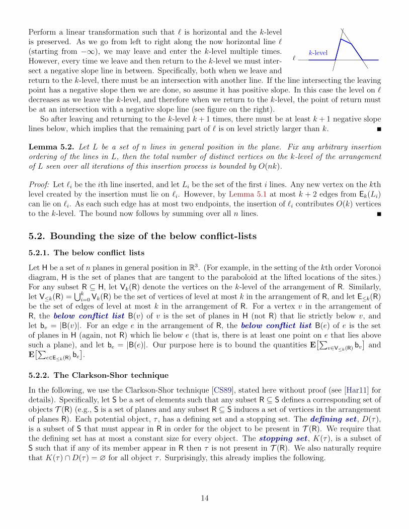
`k-level

Perform a linear transformation such that ` is horizontal and the k-levelis preserved. As we go from left to right along the now horizontal line `(starting from −∞), we may leave and enter the k-level multiple times.However, every time we leave and then return to the k-level we must inter-sect a negative slope line in between. Specifically, both when we leave andreturn to the k-level, there must be an intersection with another line. If the line intersecting the leavingpoint has a negative slope then we are done, so assume it has positive slope. In this case the level on `decreases as we leave the k-level, and therefore when we return to the k-level, the point of return mustbe at an intersection with a negative slope line (see figure on the right).

So after leaving and returning to the k-level k + 1 times, there must be at least k + 1 negative slopelines below, which implies that the remaining part of ` is on level strictly larger than k.

Lemma 5.2. Let L be a set of n lines in general position in the plane. Fix any arbitrary insertionordering of the lines in L, then the total number of distinct vertices on the k-level of the arrangementof L seen over all iterations of this insertion process is bounded by O(nk).

Proof: Let `i be the ith line inserted, and let Li be the set of the first i lines. Any new vertex on the kthlevel created by the insertion must lie on `i. However, by Lemma 5.1 at most k + 2 edges from Ek(Li)can lie on `i. As each such edge has at most two endpoints, the insertion of `i contributes O(k) verticesto the k-level. The bound now follows by summing over all n lines.

5.2. Bounding the size of the below conflict-lists

5.2.1. The below conflict lists

Let H be a set of n planes in general position in R3. (For example, in the setting of the kth order Voronoidiagram, H is the set of planes that are tangent to the paraboloid at the lifted locations of the sites.)For any subset R ⊆ H, let Vk(R) denote the vertices on the k-level of the arrangement of R. Similarly,let V≤k(R) =

⋃ki=0 Vk(R) be the set of vertices of level at most k in the arrangement of R, and let E≤k(R)

be the set of edges of level at most k in the arrangement of R. For a vertex v in the arrangement ofR, the below conflict list B(v) of v is the set of planes in H (not R) that lie strictly below v, andlet bv = |B(v)|. For an edge e in the arrangement of R, the below conflict list B(e) of e is the setof planes in H (again, not R) which lie below e (that is, there is at least one point on e that lies abovesuch a plane), and let be = |B(e)|. Our purpose here is to bound the quantities E

[∑v∈V≤k(R) bv

]and

E[∑

e∈E≤k(R) be].

5.2.2. The Clarkson-Shor technique

In the following, we use the Clarkson-Shor technique [CS89], stated here without proof (see [Har11] fordetails). Specifically, let S be a set of elements such that any subset R ⊆ S defines a corresponding set ofobjects T (R) (e.g., S is a set of planes and any subset R ⊆ S induces a set of vertices in the arrangementof planes R). Each potential object, τ , has a defining set and a stopping set. The defining set , D(τ),is a subset of S that must appear in R in order for the object to be present in T (R). We require thatthe defining set has at most a constant size for every object. The stopping set , K(τ), is a subset ofS such that if any of its member appear in R then τ is not present in T (R). We also naturally requirethat K(τ) ∩D(τ) = ∅ for all object τ . Surprisingly, this already implies the following.

14

Theorem 5.3 (Bounded Moments [CS89]). Using the above notation, let S be a set of n elements,and let R be a random sample of size r from S. Let f(·) be a monotonically increasing function boundedby a polynomial (that is, f(n) = nO(1)). We have

E

[∑τ∈T (R)

f(|K(τ)|

)]= O

(E[|T (R)|

]f(nr

)),

where the expectation is taken over random sample R.

5.2.3. Bounding the below conflict-lists

The technical challenge. The proof of the next lemma is technically interesting as it does not followin a straightforward fashion from the Clarkson-Shor technique. Indeed, the below conflict list is not thestandard conflict list. Specifically, the decision whether a vertex v in the arrangement of R is of level atmost k is a “global” decision of R, and as such the defining set of this vertex is neither of constant size,nor unique, as required to use the Clarkson-Shor technique. If this was the only issue, the extension byAgarwal et al. [AMS98] could handle this situation. However it is even worse: a plane h ∈ H \ R that isbelow a vertex v ∈ V≤k(R) is not necessarily conflicting with v (that is, in the stopping set of v) — asits addition to R will not necessarily remove v from V≤k(R ∪ h).

The solution. Since the standard technique fails in this case, we need to perform our argumentsomehow indirectly. Specifically, we use a second random sample and then deploy the Clarkson-Shortechnique on this smaller sample — this is reminiscent of the proof bounding the size of V≤k(H) byClarkson-Shor [CS89], and the proof of the exponential decay lemma of Chazelle and Friedman [CF90].

Lemma 5.4. Let k be a fixed constant, and let R be a random sample (without replacement) of size rfrom a set of H of n planes in R3, we have

E[∑

v∈V≤k(R)bv]

= O(nk3).

Proof: For the sake of simplicity of exposition, let us assume that the sampling here is done by pickingevery element into the random sample R with probability r/n. Doing the computations below usingsampling without replacement (so we get the exact size) requires modifying the calculations so that theprobabilities are stated using binomial coefficients — this makes the calculation messier, but the resultsremain the same. See [Sha03] for further discussion of this minor issue.

Fix a random sample R. Now sample once again by picking each plane in R, with probability 1/k, intoa subsample R′. Let us consider the probability that a vertex v ∈ V≤k(R) ends up on the lower envelopeof R′. A lower bound can be achieved by the standard argument of Clarkson-Shor. Specifically, if avertex v is on the lower envelope then its three defining planes must be in R′. Moreover, as v ∈ V≤k(R),by definition there are at most k planes below v that must not be in R′. So let Xv be the indicatorvariable of whether v appears on the lower envelope of R′. We then have

ER′[Xv

∣∣ R]≥ 1

k3(1− 1/k)k ≥ 1

e2k3.

Observe that

ER′

[∑v∈V0(R′)

bv

]= ER

[ER′

[∑v∈V0(R′) bv

∣∣∣ R]]≥ ER

[ER′

[∑v∈V≤k(R)Xvbv

∣∣∣ R]]. (5.1)

15

Fixing the value of R, the lower bound above implies

ER′

[∑v∈V≤k(R)

Xvbv

∣∣∣∣ R

]=

∑v∈V≤k(R)

ER′

[Xvbv

∣∣∣ R]

=∑

v∈V≤k(R)

bvER′

[Xv

∣∣∣ R]≥

∑v∈V≤k(R)

bve2k3

,

by linearity of expectations and as bv is a constant for v. Plugging this into Eq. (5.1), we have

ER′

[∑v∈V0(R′)

bv

]≥ ER

[∑v∈V≤k(R)

bve2k3

]=

1

e2k3ER

[∑v∈V≤k(R)

bv

]. (5.2)

Observe that R′ is a random sample of R which by itself is a random sample of H. As such, one caninterpret R′ as a direct random sample of H. The lower envelope of a set of planes has linear complexity,and for a vertex v on the lower envelope of R′ the set B(v) is the standard conflict list of v. As such,Theorem 5.3 implies

ER′

[∑v∈V0(R′)

bv

]= O

(|R′| · n

|R′|

)= O(n).

Plugging this into Eq. (5.2) implies the claim.

Corollary 5.5. Let R be a random sample (without replacement) of size r from a set H of n planes inR3. We have that ER

[∑e∈E≤k(R) be

]= O(nk3).

Proof: Under general position assumption every vertex in the arrangement of H is adjacent to 8 edges.For an edge e = uv, it is easy to verify that B(e) ⊆ B(u) ∪ B(v), and as such we charge the conflict listof e to its two endpoints u and v, and every vertex get charged O(1) times. Now, the claim follows byLemma 5.4.

This argument fails to capture edges that are rays in the arrangement, but this is easy to overcomeby clipping the arrangement to a bounding box that contains all the vertices of the arrangement. Weomit the easy but tedious details.

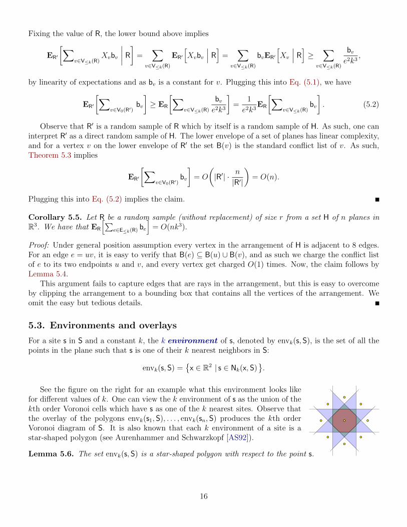
5.3. Environments and overlays

For a site s in S and a constant k, the k environment of s, denoted by envk(s, S), is the set of all thepoints in the plane such that s is one of their k nearest neighbors in S:

envk(s, S) =

x ∈ R2 | s ∈ Nk(x, S).

See the figure on the right for an example what this environment looks likefor different values of k. One can view the k environment of s as the union of thekth order Voronoi cells which have s as one of the k nearest sites. Observe thatthe overlay of the polygons envk(s1, S), . . . , envk(sn, S) produces the kth orderVoronoi diagram of S. It is also known that each k environment of a site is astar-shaped polygon (see Aurenhammer and Schwarzkopf [AS92]).

Lemma 5.6. The set envk(s, S) is a star-shaped polygon with respect to the point s.

16

Proof: Consider the set of all n− 1 bisectors determined by s and any other site in S. For any point x inthe plane, p ∈ envk(s, S) holds if the segment from s to p crosses at most k − 1 of these bisectors. Thestar-shaped property follows as when walking along any ray emanating from s, the number of bisectorscrossed is a monotonically increasing function of distance from s. Moreover, envk(s, S) is a polygon asits boundary is composed of subsets of straight line bisectors.

Going back to our original problem. Let k be a fixed constant, and let 〈s1, . . . , sn〉 be the volumeordering of S. As usual, we use Si to denote the unordered ith prefix of 〈s1, . . . , sn〉. Let envi =envk(si, Si), the union of all cells in the kth order Voronoi diagram of Si where si is one of the k nearestneighbors.

Observation 5.7. The arrangement determined by the overlay of the polygons env1, . . . , envn is the kthorder proxy diagram of S.

5.4. Putting it all together

The proof of the following lemma is similar in spirit to the argument of Har-Peled and Raichel [HR14].

Lemma 5.8. Let S be a set of n sites in the plane, let 〈s1, . . . , sn〉 be the volume ordering of S, and let kbe a fixed number. The expected complexity of the arrangement determined by the overlay of the polygonsenv1, . . . , envn (and therefore, the expected complexity of the kth order proxy diagram) is O(k4n log n),where envi = envk(si, Si) and Si = s1, . . . , si is the underlying set of the ith prefix of 〈s1, . . . , sn〉, foreach i.

Proof: As the arrangement of the overlay of the polygons env1, . . . , envn is a planar map, it suffices tobound the number of edges in the arrangement. Fix an iteration i, and observe that Si is fixed once iis fixed. For an edge e ∈ E≤k(Si), let Xe be the indicator variable of the event that e was created inthe ith iteration, and furthermore, lies on the boundary of envi. Observe that E[Xe | Si] ≤ 4/i, as anedge appears for the first time in round i only if one of its (at most) four defining sites was the ith siteinserted.

For each i, let E(envi) be the edges in E≤k(Si) that appear on the boundary of envi (for simplicitywe do not distinguish between edges in E≤k(Si) in R3 and their projection in the plane). Created in theith iteration, an edge e in E(envi) is going to be broken into several pieces in the final arrangement ofthe overlay. Let ne be the number of such pieces that arise from e.

Here we claim that ne ≤ c · kbe for some constant c. Indeed, ne counts the number of futureintersections of e with the edges of E(envj), for any j > i. As the edge e is on the k-level at the time ofcreation, and the edges in E(envj) are on the k-level when they are being created (in the future), theseedges must lie below e. Namely, any future intersect on e are caused by intersections of (pairs of) planesin B(e). So consider the intersection of all planes in B(e) on the vertical plane containing e. (Since Siis fixed, B(e) is also fixed for all e ∈ E≤k(Si).) On this vertical plane, B(e) is a set of be lines, whoseinsertion ordering is defined by the suffix of the permutation 〈si+1, . . . , sn〉. Now any edge of E(envj), forsome j > i, that intersects e must appear as a vertex on the k-level at some point during the insertionof these lines. However, by Lemma 5.2, applied to the lines of B(e) on the vertical plane of e, under anyinsertion ordering there are at most O(kbe) vertices that ever appear on the k-level.

Let Yi =∑

e∈E(envi)ne =

∑e∈E≤k(Si)

neXe be the total (forward) complexity contribution to the final

17

arrangement of edges added in round i. We thus have

E[Yi

∣∣∣ Si]

= E

[∑e∈E≤k(Si)

neXe

∣∣∣∣ Si

]≤ E

[∑e∈E≤k(Si)

ckbeXe

∣∣∣∣ Si

]=∑

e∈E≤k(Si)ckbe E

[Xe

∣∣∣ Si]≤ 4ck

i·∑

e∈E≤k(Si)be.

The total complexity of the overlay arrangement of the polygons env1, . . . , envn is asymptoticallybounded by

∑i Yi, and so by Corollary 5.5 we have

E[∑

i Yi

]=∑i

E

[E[Yi

∣∣∣ Si]]≤∑i

E

[4ck

i·∑

e∈E≤k(Si)be

]= O

(∑i

nk4

i

)= O

(k4n log n

).

6. On the expected size of the staircase

6.1. Number of staircase points

6.1.1. The two dimensional case

Corollary 6.1. Let P be a set of n points sampled uniformly at random from the unit square [0, 1]2.Then the number of staircase points (P) in P is Owhp(log n).

Proof: If we order the points in P by increasing x-coordinate, then the staircase points are exactlythe points which have the smallest y-values out of all points in their prefix in this ordering. As thex-coordinates are sampled uniformly at random, this ordering is a random permutation 〈y1, . . . , yn〉of the y-values Y. Let Xi be the indicator variable of the event that yi is the smallest number inYi = y1, . . . , yi for each i. By setting property P(Yi) to be the smallest number in the prefix Yi, wehave

∑ni=1Xi = O(log n) with high probability by Corollary 3.1.

6.1.2. Higher dimensions

Lemma 6.2. Fix a dimension d ≥ 2. Let m and n be parameters, such that m ≤ n. Let Q =〈q1, . . . , qm〉 be an ordered set of m points picked randomly from [0, 1]d as described in Section 2.2.Assume that we have

∣∣ (Qi)∣∣ = O(cd logd−1 n), with high probability with respect to m for all i simulta-

neously, where Qi = q1, . . . , qi is the underlying set of the ith prefix of Q. Then, the set =⋃mi=1 (Qi)

has size O(cd logd n), with high probability with respect to m.

Proof: Let∣∣ (Qi)

∣∣ ≤ c′ ·cd lnd−1 n with probability 1−m−c for large enough constant c and some constantc′ depending on c. By setting P(Qi) = (Qi), we have that Pr

[∣∣ ∣∣ > γ(2k lnm)]≤ m−γk + m−c for

k = c′ · cd lnd−1 n and any γ ≥ 2e, by Corollary 3.1. Setting γ = 2e lnn/ lnm implies the claim.

Lemma 6.3. Fix a dimension d ≥ 2. Let m,n be parameters, such that m ≤ n. Let P be a set of mpoints picked randomly from [0, 1]d as described in Section 2.2. Then,

∣∣ (P)∣∣ = O(cd logd−1 n) holds,

with high probability with respect to m, for some constant cd that depends only on d.

18

Proof: The argument follows by induction on dimension. The two-dimensional case follows from Corol-lary 6.1. Assume we have proven the claim for all dimension smaller than d.

Now, sort P by increasing value of the dth coordinate, and let pi = (qi, `i) be the ith point in P inthis order for each i, where qi is a (d − 1)-dimensional vector and `i is the value of the dth coordinateof pi. Observe that the points q1, . . . , qm are randomly, uniformly, and independently picked from thehypercube [0, 1]d−1. Now, if pi is a minima point of P, then it is a minima point of p1, . . . , pi. Butthis implies that qi is a minima point of Qi = q1, . . . , qi as well. Namely, qi ∈ =

⋃mi=1 (Qi). This

implies that∣∣ (P)

∣∣ ≤ ∣∣ ∣∣. Now, applying induction hypothesis on each Qi in dimension d− 1 we have∣∣ (Qi)∣∣ = O(cd−1 logd−2 n) holds for all i, with high probability with respect to m. Plugging it into

Lemma 6.2 we have∣∣ (P)

∣∣ ≤ ∣∣ ∣∣ = O(cd−1 logd−1 n), with high probability with respect to m. Choosinga proper constant cd now implies the claim.

Lemma 6.4. Fix a dimension d ≥ 2. Let Q = 〈q1, . . . , qn〉 be an ordered set of n points picked randomlyfrom [0, 1]d (as described in Section 2.2), and Qi = q1, . . . , qi is the ith (unordered) prefix of Q. Then,the set

⋃ni=1 (Qi) is of size Owhp(cd logd n), and the staircase (P) is of size Owhp(cd logd−1 n).

Proof: By Lemma 6.2, the set⋃ni=1 (Qi) is of size O(cd logd n), with high probability. By Lemma 6.3,

the set (P) is of size O(cd logd−1 n), with high probability.

Remark 6.5. In the proof of Lemma 6.3 whether a point is on the staircase (or not) only depends on thecoordinate orderings of the points and not their actual values.

The basic recursive argument used in Lemma 6.3 was used by Clarkson [Cla04] to bound the expectednumber of k-sets for a random point set. Here, using Corollary 3.1 enables us to get a high-probabilitybound.

Note that the definition of the staircase can be made with respect to any corner of the hypercube(that is, this corner would replace the origin in the definition dominance, point volume, the exponentialgrid, etc). Taking the union over all 2d such staircases gives us the subset of P on the orthogonal convexhull of P. Therefore Lemma 6.4 also bounds the number of input points on the orthogonal convex hull.As the vertices on the convex hull of P are a subset of the points in P on the orthogonal convex hull,the above also implies the same bound on the number of vertices on the convex hull.

6.2. Bounding the size of the candidate set

We can now readily bound the size of the candidate set for any point in the plane.

Lemma 6.6. Let S be a set of n sites in the plane, where for each site s in S, a parametric point froma distribution over [0, 1]d is sampled (as described in Section 2.2). Then, the candidate set has sizeOwhp(logd n) simultaneously for all points in the plane.

Proof: Consider the arrangement of bisectors of all pairs of points of S. This arrangement has com-plexity O(n4), and inside each cell the candidate set is the same. Now for any point in a cell of thearrangement, Lemma 6.4 immediately gives us the stated bound, with high probability. Therefore pick-ing a representative point from each cell in this arrangement and applying the union bound imply theclaim.

19

7. The main result

We now use the bound on the complexity of the proxy diagram, as well as our knowledge of therelationship between the candidate set and the proxy set to bound the complexity, as well as the spacecomplexity, of the candidate diagram.

Recall that the complexity of a candidate diagram, treated as a planar arrangement, is the totalnumber of edges, faces, and vertices in the diagram. The space complexity of the candidate diagram isthe sum of the sizes of candidate sets over all the faces in the arrangement of the diagram.

Theorem 7.1. Let S be a set of n sites in the plane, where for each site in S we sample an associatedparametric point in [0, 1]d, as described in Section 2.2. Then, the expected complexity of the candidatediagram is O

(n log8d+5 n

). The expected space complexity of this candidate diagram is O

(n log9d+5 n

).

Proof: Fix k to be sufficiently large such that k = Θ(logd n). By Lemma 5.8 the expected complexity ofthe proxy diagram is O(k4n log n). Triangulating each polygonal cell in the diagram does not increase itsasymptotic complexity. Lemma 4.2 implies that, the proxy set has size Owhp(k log n) simultaneously forall the points in the plane. Now, Lemma 4.4 implies that, with high probability, the proxy set containsthe candidate set for any point in the plane.

The resulting triangulation has O(k4n log n) faces, and inside each face all the sites that mightappear in the candidate set are all present in the proxy set of this face. By Lemma 2.4, the complexityof an m-site candidate diagram is O(m4). Therefore the complexity of the candidate diagram per faceis Owhp((k log n)4) (clipping the candidate diagram of these sites to the containing triangle does notincrease the asymptotic complexity). Multiplying the number of faces, O(k4n log n), by the complexityof the arrangement within each face, O((k log n)4), yields the desired result.

The bound on the space complexity follows readily from the bound on the size of the candidate setfrom Lemma 6.6.

Acknowledgments

The authors would like to thank Pankaj Agarwal, Ken Clarkson, Nirman Kumar, and Raimund Seidelfor useful discussions related to this work. We are also grateful to the anonymous SoCG reviewers fortheir helpful comments.

References

[AAH+13] P. K. Agarwal, B. Aronov, S. Har-Peled, J. M. Phillips, K. Yi, and W. Zhang. Nearestneighbor searching under uncertainty II. In Proc. 32nd ACM Sympos. Principles DatabaseSyst. (PODS), pages 115–126, 2013.

[AHKS14] P. K. Agarwal, S. Har-Peled, H. Kaplan, and M. Sharir. Union of random minkowski sumsand network vulnerability analysis. Discrete Comput. Geom., 52(3):551–582, 2014.

[AKL13] F. Aurenhammer, R. Klein, and D.-T. Lee. Voronoi Diagrams and Delaunay Triangulations.World Scientific, 2013.

[AMS98] P. K. Agarwal, J. Matousek, and O. Schwarzkopf. Computing many faces in arrangementsof lines and segments. SIAM J. Comput., 27(2):491–505, 1998.

20

[AS92] F. Aurenhammer and O. Schwarzkopf. A simple on-line randomized incremental algorithmfor computing higher order Voronoi diagrams. Internat. J. Comput. Geom. Appl., pages363–381, 1992.

[BCKO08] M. de Berg, O. Cheong, M. van Kreveld, and M. H. Overmars. Computational Geometry:Algorithms and Applications. Springer-Verlag, 3rd edition, 2008.

[BDHT05] Z.-D. Bai, L. Devroye, H.-K. Hwang, and T.-H. Tsai. Maxima in hypercubes. RandomStruct. Alg., 27(3):290–309, 2005.

[BKS01] S. Borzsonyi, D. Kossmann, and K. Stocker. The skyline operator. In Proc. 17th IEEE Int.Conf. Data Eng., pages 421–430, 2001.

[BKST78] J. L. Bentley, H. T. Kung, M. Schkolnick, and C. D. Thompson. On the average number ofmaxima in a set of vectors and applications. J. Assoc. Comput. Mach., 25(4):536–543, 1978.

[BR10a] I. Barany and M. Reitzner. On the variance of random polytopes. Adv. Math., 225(4):1986–2001, 2010.

[BR10b] I. Barany and M. Reitzner. Poisson polytopes. Annals. Prob., 38(4):1507–1531, 2010.

[CF90] B. Chazelle and J. Friedman. A deterministic view of random sampling and its use ingeometry. Combinatorica, 10(3):229–249, 1990.

[CHPR14] Hsien-Chih Chang, Sariel Har-Peled, and Benjamin Raichel. From proximity to utility: AVoronoi partition of Pareto optima. CoRR, abs/1404.3403, 2014.

[CHPR15] Hsien-Chih Chang, Sariel Har-Peled, and Benjamin Raichel. From proximity to utility: AVoronoi partition of Pareto optima. In 31st International Symposium on ComputationalGeometry (SoCG 2015), volume 34, pages 689–703, 2015.

[Cla04] K. L. Clarkson. On the expected number of k-sets of coordinate-wise independent points.manuscript, 2004.

[CMS93] K. L. Clarkson, K. Mehlhorn, and R. Seidel. Four results on randomized incremental con-structions. Comput. Geom. Theory Appl., 3(4):185–212, 1993.

[CS89] K. L. Clarkson and P. W. Shor. Applications of random sampling in computational geometry,II. Discrete Comput. Geom., 4:387–421, 1989.

[Fel08] A. Feldman. Welfare economics. In S. Durlauf and L. Blume, editors, The New PalgraveDictionary of Economics. Palgrave Macmillan, 2008.

[GSG07] P. Godfrey, R. Shipley, and J. Gryz. Algorithms and analyses for maximal vector computa-tion. VLDB J., 16(1):5–28, 2007.

[Har11] S. Har-Peled. Geometric Approximation Algorithms, Volume 173 of Mathematical Surveysand Monographs. Amer. Math. Soc., 2011.

[HR14] S. Har-Peled and B. Raichel. On the expected complexity of randomly weighted Voronoidiagrams. In Proc. 30th Annu. Sympos. Comput. Geom. (SoCG), pages 232–241, 2014.

21

[HTC13] H.-K. Hwang, T.-H. Tsai, and W.-M. Chen. Threshold phenomena in k-dominant skylinesof random samples. SIAM J. Comput., 42(2):405–441, 2013.

[HW87] D. Haussler and E. Welzl. ε-nets and simplex range queries. Discrete Comput. Geom.,2:127–151, 1987.

[KLP75] H. Kung, F. Luccio, and F. Preparata. On finding the maxima of a set of vectors. J. Assoc.Comput. Mach., 22(4):469–476, 1975.

[OSW84] T. Ottmann, E. Soisalon-Soininen, and D. Wood. On the definition and computation ofrectlinear convex hulls. Inf. Sci., 33(3):157–171, 1984.

[SA95] M. Sharir and P. K. Agarwal. Davenport-Schinzel Sequences and Their Geometric Applica-tions. Cambridge University Press, New York, 1995.

[Sei93] R. Seidel. Backwards analysis of randomized geometric algorithms. In J. Pach, editor, NewTrends in Discrete and Computational Geometry, volume 10 of Algorithms and Combina-torics, pages 37–68. Springer-Verlag, 1993.

[Sha03] M. Sharir. The Clarkson-Shor technique revisited and extended. Comb., Prob. & Comput.,12(2):191–201, 2003.

[SW93] R. Schneider and J. A. Wieacker. Integral geometry. In P. M. Gruber and J. M. Wills,editors, Handbook of Convex Geometry, volume B, chapter 5.1, pages 1349–1390. North-Holland, 1993.

[WW93] W. Weil and J. A. Wieacker. Stochastic geometry. In P. M. Gruber and J. M. Wills, editors,Handbook of Convex Geometry, volume B, chapter 5.2, pages 1393–1438. North-Holland,1993.

A. An Integral Calculation

Lemma A.1. Let Fd(∆) be the total measure of the points p = (p1, . . . , pd) in the hypercube [0, 1]d, suchthat pv(p) = p1p2 · · · pd ≤ ∆. That is, Fd(∆) is the measure of all points in hypercube with point volumeat most ∆. Then

Fd(∆) =d−1∑i=0

∆

i!lni

1

∆.

Proof: The claim follows by tedious but relatively standard calculations. As such, the proof is includedfor the sake of completeness.

(1,∆)

(∆, 1)

∆

The case for d = 1 is trivial. Consider the d = 2 case. Here the points whosepoint volume equals ∆ are defined by the curve xy = ∆. This curve intersectsthe unit square at the point (∆, 1). As Fd(∆) is the total volume under this curvein the unit square we have that

F2(∆) = ∆ +

∫ 1

x=∆

∆

xdx = ∆ + ∆ ln

1

∆.

22

In general, we have

1

(d− 1)!

∫ 1

x=∆

∆

xlnd−1 x

∆dx =

∆

(d− 1)!

[1

dlnd

x

∆

]1

x=∆

=∆

d!lnd

1

∆.

Now assume inductively that

Fd−1(∆) =d−2∑i=0

1

i!∆ lni

1

∆,

then we have

Fd(∆) = ∆ +

∫ 1

xd=∆

Fd−1

(∆

xd

)dxd = ∆ +

∫ 1

xd=∆

(d−2∑i=0

∆

i!xdlni

xd∆

)dxd

= ∆ +d−2∑i=0

1

i!

(∫ 1

xd=∆

∆

xdlni

xd∆

dxd

)= ∆ +

d−1∑i=1

∆

i!lni

1

∆=

d−1∑i=0

∆

i!lni

1

∆.

23