from market making to matchmaking: does bank regulation
TRANSCRIPT

From Market Making to Matchmaking:Does Bank Regulation Harm Market Liquidity?
Gideon Saar, Jian Sun, Ron Yang, and Haoxiang Zhu∗
This version: September 2020
Abstract
Post-crisis bank regulations raised market-making costs for bank-affiliated dealers. We show that
this can, somewhat surprisingly, improve overall investor welfare and reduce average transaction
costs despite the increased cost of immediacy. Bank dealers in OTC markets optimize between
two parallel trading mechanisms: market making and matchmaking. Bank regulations that
increase market-making costs change the market structure by intensifying competitive pressure
from non-bank dealers and incentivizing bank dealers to shift their business toward matchmaking.
Thus, post-crisis bank regulations have the (unintended) benefit of replacing costly bank balance
sheets with a more efficient form of financial intermediation.
Keywords: bank regulation, market making, matchmaking, financial crisis, corporate bonds, liquidity,
over-the-counter markets, broker-dealers, Basel 2.5, Basel III, Volcker Rule, post-crisis regulation,
market microstructure
JEL Classification: G01, G12, G21, G24, G28
∗Gideon Saar is from the Johnson Graduate School of Management, Cornell University ([email protected]). JianSun is from MIT Sloan School of Management ([email protected]). Ron Yang is from Harvard Business School([email protected]). Haoxiang Zhu is from MIT Sloan School of Management and the NBER ([email protected]).We thank Philip Bond, Briana Chang, Christopher Hrdlicka, Stacey Jacobsen, Pete Kyle, Jonah Platt, DimitriVayanos, Kumar Venkataraman, Yajun Wang, Yao Zeng, Zhuo Zhong, and Hao Zhou as well as seminar/conferenceparticipants at the American Finance Association 2020 meeting, the Chinese University of Hong Kong, the ChineseUniversity of Hong Kong Shenzhen, the City University of Hong Kong, Cornell University, the Financial IndustryRegulatory Authority, Manchester Business School, MIT, the PBC School of Finance, University at Buffalo, theUniversity of British Columbia, the University of Illinois, the University of Washington, Warwick Business School,Wharton, the 4th Sydney Market Microstructure Meeting, and the mini-conference on Regulatory Reform at theUniversity of Wisconsin-Madison for helpful comments.
1 Introduction
The aftermath of the financial crisis saw several regulatory initiatives to curtail banks’ risk-taking
desire, hindering proprietary trading and increasing the cost of market making. In part, these
initiatives reflected a widespread belief in banking regulatory circles that the pre-crisis price of
immediacy did not adequately incorporate the costs required to ensure that market makers are
supported by sufficient capital and do not become a source of illiquidity contagion (see, for example,
BIS Committee on the Global Financial System (2014, 2016)). While the regulations were meant
to improve market-maker resilience, the post-crisis changes in the Basel framework (Basel 2.5 and
Basel III) and the Volcker Rule have reduced banks’ willingness to accommodate corporate bond
trades on their balance sheets and in general have made their market-making operations more
costly. Some market observers have portrayed these regulatory initiatives in the light of a trade-off
between market resilience (less severe contagion) in times of stress and liquidity during normal
times. Reduced market liquidity during normal times, as the argument goes, may be a necessary
compromise for enhanced market resilience during stressful periods.
Such a perspective, however, overlooks the market microstructure aspect of liquidity. In
particular, the over-the-counter corporate bond market features two parallel trading mechanisms
corresponding to the dual capacity of broker-dealers. In the first mechanism, market making, a bank
intermediary functions as a dealer that provides immediacy to customers by taking bonds onto his
balance sheet. In the second mechanism, matchmaking, a bank intermediary functions as a broker
that searches for couterparties for her customers.1 While regulations aimed at boosting market
resilience increased the cost of taking a bond onto a bank’s balance sheet, they did not increase the
costs associated with the process of matching customers. In fact, technological innovations over the
past two decades have reduced the costs of matching, making this trading mechanism an attractive
option. Our focus in this paper is therefore not on the trade-off between resilience in times of stress
and liquidity during normal times. Rather, we investigate whether the regulatory push to increase
resilience could make investors better off during normal times by changing the market structure
they experience when trading over-the-counter securities such as corporate bonds.
1The matchmaking mechanism therefore encompasses both “agency trades” and “riskless principal trades.”
1
A growing body of empirical literature investigates the impact of post-crisis regulation on
liquidity. The US corporate bond market is the most commonly studied in this context given
its large size and dealer-centric nature. On balance, this literature finds improvement or at least no
deterioration in the average transaction costs of corporate bond trades (Mizrach (2015), Adrian,
Fleming, Shachar, and Vogt (2017), Anderson and Stulz (2017), Bessembinder, Jacobsen, Maxwell,
and Venkataraman (2018), and Trebbi and Xiao (2019)). Still, some papers document an increase
in the cost of immediacy or transacting in times of stress (Bao, O’Hara, and Zhou (2018), Choi and
Huh (2017), and Dick-Nielsen and Rossi (2018)). These studies also find a reduction in the amount
of capital that bank dealers commit to market making and a shift in their activity from market
making towards matchmaking (Bao, O’Hara, and Zhou (2018), Bessembinder, Jacobsen, Maxwell,
and Venkataraman (2018), and Choi and Huh (2017)). In contrast, non-bank dealers appear to
increase capital commitments and principal trading.
While the increase in the cost of immediacy is consistent with the regulation-induced higher cost
of taking bonds onto banks’ balance sheets, the decline in average transaction costs could suggest
that a shift from market making to matchmaking is beneficial to customers. Yet, transaction costs
are an incomplete measure of overall customer welfare because of two less measurable but potentially
important costs. First, the average time it takes to execute a transaction in the post-regulation era
is likely longer. These execution delays may be costly to investors. Second, realized transaction
costs capture only trades that were executed. If customers forgo transacting in response to the
higher costs of immediacy (and their unwillingness to wait longer for execution), their welfare loss
cannot be ascertained by analyzing executed trades. To assess overall customer welfare, which is
difficult to measure empirically, one needs a model in which the trade-off between the cost of delay
(matchmaking) and the cost of immediacy (market making) is considered explicitly, and customers
have the option to forgo trading altogether. This is the model we set out to investigate.
Our model features infinitesimal customers (buyers and sellers) who arrive at a constant rate
and wish to trade bonds in an over-the-counter market. There are two representative broker-dealers
standing for two groups of dealers: bank-affiliated dealers and non-bank-affiliated dealers. Our use
of a representative bank dealer and a representative non-bank dealer is meant to acknowledge the
2

market power dealers possess in the corporate bond market relative to customers while at the same
time enabling us to explicitly consider the changing nature of competition between the two broker-
dealer groups as a result of bank regulations. The bank dealer offers his customers two mechanisms
for trading bonds. The first, market making, enables customers to trade immediately at a spread
that reflects the bank dealer’s cost of market making. In the second, matchmaking, the bank dealer
helps customers search for trading counterparties and earns a fee to facilitate such trades.
The bank dealer optimally sets the market-making spread and the matchmaking fee by taking
into account his balance sheet cost as well as the search cost and matching rate in the matchmaking
mechanism. The non-bank dealer offers market-making services to customers at a spread that he
sets to reflect his cost of market making and the competitive environment.2 The balance sheet costs
of the bank dealer and the non-bank dealer are generally different. Customers are price takers and
heterogeneous with regard to patience (or the value they attach to immediacy), which we model
with private values. They optimize over their trading choices: trade immediately with the bank
dealer, trade immediately with the non-bank dealer, use the matchmaking service of the bank dealer
and incur delay costs, or forgo trading altogether.
Our main analysis focuses on how customer welfare and market outcomes change when regulation
increases the bank dealer’s balance sheet cost. If the cost of market making of the bank dealer is
lower than that of the non-bank dealer, there are two types of equilibria, depending on whether the
bank dealer’s spread is constrained by competition from the non-bank dealer. In the unconstrained
equilibrium, any increase in the balance sheet cost of the bank dealer is fully passed on to customers,
harming customer welfare. This result is reminiscent of warnings made by some market observers
that raising the costs of banks would hurt investors in the corporate bond market.
The aforementioned equilibrium is, however, far from providing the complete picture. The more
prevalent equilibrium in our model—the constrained bank dealer equilibrium—has a completely
different flavor. In this equilibrium, the bank dealer’s ability to pass the increase in balance sheet
costs on to the customers is constrained by the competitive pressure in market making from the
non-bank dealer. A higher balance sheet cost therefore incentivizes the bank dealer to shift more of
2Non-bank dealers are typically smaller and are not subject to bank regulations that increase balance sheet costs(Bao, O’Hara, and Zhou (2018), Bessembinder, Jacobsen, Maxwell, and Venkataraman (2018)).
3

his business to the matchmaking mechanism. As a result, overall customer welfare, which takes into
account not just transaction costs but also waiting costs and the welfare of customers who choose
not to trade, unambiguously rises. The welfare improvement in the constrained bank equilibrium
is driven by the lower matchmaking fee that attracts new customers to trade and benefits all those
who use the matchmaking service.
If the balance sheet cost of the bank dealer rises above that of the non-bank dealer, however,
customers who demand immediacy switch to the non-bank dealer. The bank dealer, in turn, focuses
on maximizing profits in the matchmaking mechanism alone. In this region, increases in regulatory
costs reduce the potential for competition between the two representative dealers and therefore
result in lower overall customer welfare. Hence, the relationship between the balance sheet costs of
the bank and non-bank dealers, which determines the extent to which they influence each other’s
pricing, is very important to the manner in which overall customer welfare responds to changes in
bank regulatory costs in each equilibrium region. The industrial organization aspect, manifested as
competitive pressure from the non-bank dealer, and the market microstructure perspective, which
introduces possible substitution between the two trading mechanisms, join to deliver the richness
of our implications. They are two of the key drivers behind the result that the increase in bank
dealer’s cost can make customers better off.
The third key driver that is crucial for our results is that bank dealers possess market power
relative to customers. This market power impacts both how customer welfare changes in response to
increased regulatory costs and the division of the surplus created by technological innovations that
have reduced search costs in the matchmaking mechanism over the last two decades. We find that
lower search costs unambiguously increase overall customer welfare only in the constrained bank
dealer equilibrium. When the bank dealer has unconstrained monopoly power over the provision
of market making, the surplus generated by lower search costs can predominantly benefit the bank
dealer.
Given the central role played by the market power of bank dealers in both the corporate bond
market and our model, we investigate the robustness of our conclusions by analyzing a variant of
the model with multiple bank dealers and using the extent of differentiation among the bank dealers
4
to vary the amount of market power they possess relative to customers. We find that increasing
regulatory costs can improve overall customer welfare as long as bank dealers have even a small
amount of market power, and the parameter region over which this improvement occurs increases
in the bank dealers’ market power. In other words, only if bank dealers were perfectly competitive
would an increase in regulatory costs always lower overall customer welfare, but the evidence in
bond markets resoundingly rejects the notion that bank dealers are perfectly competitive.
Our model demonstrates the complex and interesting economic interactions that evolve as bank
regulatory costs increase, pointing to subtleties not fully recognized in the extant literature. Our
contribution lies in characterizing how changes in bank regulatory costs, both in absolute terms
and relative to the market-making costs of non-bank dealers, affect the nature of equilibrium in
the market, with each equilibrium region giving rise to a set of implications for customer welfare
and market outcomes. These complex interactions also highlight why empirical work thus far has
struggled to articulate the overall impact of increased bank regulatory costs on customer welfare
in the corporate bond market.
Can our theory contribute to evaluating how the post-crisis regulatory initiatives impacted
customer welfare in the corporate bond market? We address this question by relating the wealth
of empirical implications generated by the model to findings reported in empirical papers. As we
increase bank regulatory costs in the model, our predictions for observable market outcomes change
as we move from one equilibrium region to another. We believe that the patterns uncovered by the
empirical literature suggest that the suite of post-crisis bank regulations has moved the corporate
bond market into and across the constrained bank dealer equilibrium region in which an increase
in bank regulatory costs improves overall customer welfare.3 While bank dealers are clearly worse
off in the post-crisis regulatory environment, our model vividly demonstrates that regulations that
negatively impact dealer profitability and capital commitment need not translate into lower overall
customer welfare.
The regulation of banks’ proprietary trading remains a work in progress. In 2019, for example,
3It is important to stress that the empirical patterns documented in these papers reflect the overall effects ofpost-crisis regulations. Hence, our results do not imply that a particular rule (or any specific feature of a particularrule) is beneficial for customer welfare.
5

the five agencies responsible for administering the Volcker Rule approved changes in the rule. While
most of the changes appear to be focused on simplifying reporting as opposed to significantly altering
the operations of bank trading desks, some have the potential to affect market-making incentives.
We believe that understanding how bank regulations that change the cost of market making impact
customer welfare and the functioning of the corporate bond market is of paramount importance.
We hope that our insights shed clarifying light on this important question.
2 Background and Literature
2.1 Post-Crisis Bank Regulations and the Corporate Bond Market
The Basel regulatory framework and the Dodd-Frank Act are the cornerstones of post-crisis bank
regulations that heavily impacted market-making activities in the United States, including in the
corporate bond market. Interviews with market participants suggest that the revision of the Basel
II market-risk framework (“Basel 2.5”), finalized in June 2012 in the United States, increased
inventory costs for corporate bonds by boosting regulatory capital charges through the incremental
risk capital (IRC) charge and the trading book’s stressed VaR requirement (BIS Committee on the
Global Financial System (2014)). Furthermore, the Basel III framework, finalized in July 2013 in
the United States, not only raised the risk-based capital requirements on banks but also raised the
non-risk-based capital requirement through the supplementary leverage ratio (SLR). For example,
global systemically important banks (G-SIBs) are required to maintain an SLR of 5% or higher at
the bank-holding-company level and an SLR of 6% or higher at the depository-subsidiary level (see
Davis Polk (2014) for more details). Greenwood, Hanson, Stein, and Sunderam (2017) and Duffie
(2018) find that the leverage ratio requirement is the most tightly binding constraint for most U.S.
G-SIBs, according to data derived from the Federal Reserve’s stress tests in 2017. Results from the
2019 Dodd-Frank Stress test show that the leverage ratio remains the most binding constraint for
the largest U.S. banks.4 In addition to capital requirements, another pillar of Basel III is higher
liquidity standards, including the liquidity coverage ratio (LCR) and the net stable funding ratio
4See https://www.federalreserve.gov/publications/files/2019-dfast-results-20190621.pdf.
6

(NSFR), which require that banks should hold enough high-quality liquid assets and use sufficiently
stable financing sources to guard against adverse conditions in the funding markets.
Another major regulatory measure impacting the corporate bond market is the Volcker Rule.
While the Dodd-Frank Act was signed into law in July 2010, the implementation of the Volcker
Rule was delayed until April 2014, with full compliance required by July 2015. The Volcker Rule
aims at discouraging banks with access to FDIC insurance or the Federal Reserve’s discount window
from engaging in proprietary trading of risky securities. While it provides an exception for market
making, the distinction between market making and proprietary trading is inherently blurry. The
rule, therefore, mandates the reporting of various measures (e.g., inventory turnover, the standard
deviation of daily trading profits, the customer-facing trade ratio) as proxies for the underlying
motive behind the trades. The Volcker Rule’s restrictions and associated compliance work have
increased the market-making costs that bank-affiliated dealers incur.5
By strengthening banks’ resilience to various risks (e.g., market, counterparty credit, and
funding), the suite of post-crisis bank regulations now in place changes the economics of trading
activities undertaken by banks, including market making. Some market participants therefore
warned that these rules would increase transaction costs in the corporate bond market, and these
claims motivated subsequent empirical research examining post-crisis changes in corporate bond
liquidity.
2.2 Post-Crisis Changes in Corporate Bond Liquidity: Empirical Evidence
Most empirical papers that examine corporate bond market liquidity following the financial crisis
find no deterioration, indeed even improvement, in liquidity subsequent to the regulatory interventions.
For example, Mizrach (2015) and Adrian, Fleming, Shachar, and Vogt (2017) find that measures
of execution costs dropped after the crisis to below pre-crisis levels. Adrian et al. also find that
5The regulatory costs we model in this paper probably best represent the explicit costs imposed by the Baselframework. In fact, an informal survey of market makers in the corporate bond market conducted by the Bank forInternational Settlements found that “. . . revisions to the Basel II market risk framework (Basel 2.5) were seen tohave had the largest impact on regulatory charges” (BIS Committee on the Global Financial System (2016)). Still,most empirical findings concerning the impact of post-crisis regulations on the corporate bond market reflect thecombined effects brought about by all these rules and therefore we model a single regulatory cost of market makingrather than investigating specific features of these rules.
7

trading volume and issuance are at record levels, although trade size and turnover have declined.
Anderson and Stulz (2017) look at a variety of price-based measures of liquidity, and find that
they are marginally better following the onset of regulation (2013-2014) relative to before the
crisis. Bessembinder, Jacobsen, Maxwell, and Venkataraman (2018) also document that average
customer trade execution costs have not increased after these regulations were imposed. Trebbi
and Xiao (2019) look for a structural break in various liquidity measures but find no evidence
of deteriorating liquidity during the period that corresponds to the Dodd-Frank and Basel III
regulatory interventions.6
Several papers find worsening in a particular dimension of trade execution: the cost of immediacy.
Bao, O’Hara, and Zhou (2018) use downgrades of bonds to junk status as stress events to examine
the cost of immediacy, and find that it increased following the implementation of the Volcker Rule.
Similarly, Dick-Nielsen and Rossi (2018) use exclusions from the Barclays Capital investment-grade
bond index as events that create demand for immediacy, and document an increase in the cost of
immediacy after the financial crisis. Choi and Huh (2017) show that trading costs for market-
making trades increased substantially in the post-regulation period relative to pre-crisis levels, and
this increase is driven by bank dealers.
Our model is able to reconcile these two seemingly conflicting lines of empirical evidence, namely
that average transaction costs in corporate bonds have declined while the cost of immediacy has
gone up. The driving force behind these results in our theory is the bank dealers’ endogenous shift
from market making to matchmaking. The empirical papers we have cited indeed provide ample
evidence that matchmaking has increased following the crisis and the implementation of post-crisis
regulations (e.g., Bao, O’Hara, and Zhou (2018), Choi and Huh (2017), Schultz (2017)).7 As a
result of the shift to matchmaking, the execution of large trades now tends to require more time
(BIS Committee on the Global Financial System (2014, 2016)).
6Two papers find more nuanced effects. Allahrakha, Cetina, Munyan, and Watugala (2019) find higher markupsfor a subset of the trades when looking at Volcker Rule exemptions (e.g., trades in newly issued bonds for which abank dealer is part of the bond’s underwriting group) to infer cost differentials. Chernenko and Sunderam (2018)develop an indirect measure of aggregate corporate bond market liquidity by relating mutual funds’ cash holdingsto the volatility of their fund flows. They find that, while the liquidity of investment-grade bonds in the post-crisisperiod essentially recovered to the pre-crisis level, liquidity for speculative grade bonds has not.
7Ederington, Guan, and Yadav (2014), Randall (2015), and Anand, Jotikasthira, and Venkataraman (2020) provideadditional evidence about matchmaking and the provision of liquidity by customers in the corporate bond market.
8

It is important to stress the heterogeneous manner in which bank dealers and non-bank dealers
responded to the regulatory changes. Bao, O’Hara, and Zhou (2018) find that dealers affected by the
Volcker Rule increase their matchmaking activity while committing less capital to market making.
Goldstein and Hotchkiss (2020) investigate the trades that dealers seek to offset in comparison with
those that they hold in inventory overnight. At the same time, competition in market making from
smaller non-bank dealers appears to intensify: they increase capital commitments and the amount
of principal trading (see also Bessembinder, Jacobsen, Maxwell, and Venkataraman (2018)). Non-
bank-dealer matchmaking, on the other hand, has decreased after the implementation of the Volcker
Rule. We return to the findings of the empirical literature to motivate our modeling approach and
guide our discussion of how bank regulations following the financial crisis affected customer welfare.
2.3 Market Making versus Matchmaking: Theory
Several recent theoretical papers recognize the importance of the dual mechanisms for trading
bonds, namely market making and matchmaking, although each of these papers adopts a distinct
approach to studying the two mechanisms. An, Song, and Zhang (2017) study intermediation
chains by modeling the interaction between one seller, a finite number of dealers, and an infinite
number of buyers. Their model shows how an intermediary rat race gives rise to an inefficient
amount of principal trading. Our paper does not feature an inter-dealer market or intermediation
chains, but rather focuses on what happens to customer welfare and the market environment if the
cost of market making increases for bank dealers.
An and Zheng (2017) look at how the dual capacity of broker-dealers (principal and agency
trading) gives rise to a conflict of interest, which results in dealers’ holding too much inventory as a
tool for extracting rent from customers. Unlike in our framework, customers in their model do not
optimize and matchmaking is effortless and costless, leading An and Zheng to focus on inventory as
a strategic variable. In contrast, we model a two-way market with balanced customer order flows
and abstract away from inventory management—an approach that is orthogonal to that of An and
Zheng (2017). Furthermore, we investigate the endogenous evolution of trading mechanisms by (i)
having customers optimally choose whether and how to trade and (ii) having dealers optimize the
9

pricing of their services.
Li and Li (2017) model a trade-off between inventory costs (in market making) and verification
costs (in matchmaking). Moral hazard in matchmaking arises in their model when a dealer gains by
providing worse executions for a customer. Because dealers have better information than customers,
transparency influences the prevalence of market making over matchmaking.8 Transparency plays
no role in our model because we assume homogeneous common-value information. Our emphasis,
instead, is on competition from non-bank dealers and the role it plays in determining customer
welfare and the extent of matchmaking.9
The paper closest to ours in objective is Cimon and Garriott (2019). In their model, market
makers compete for quantity (Cournot) in separate buyer and seller markets and issue equity and
debt to fund their operations. Market making is modeled as a more efficient form of trading than
matchmaking, and therefore increased agency trading implies a higher price impact of trades. As a
result, regulations that increase the cost of market making must hurt liquidity. In contrast, we show
that investment in technology can make matchmaking a less expensive form of intermediation than
market making, and the market power of dealers provides a role for bank regulations in enhancing
competition and improving customer welfare.
Our model shares certain features that are examined in the vast industrial organization (IO)
literature, in particular the branch that investigates multiproduct competition. To the best of our
knowledge, however, no other paper captures all the important characteristics of bond markets that
we wish to model. Mussa and Rosen (1978) characterize the optimal pricing strategy of a monopolist
over a range of products that differ in quality. Katz (1984) analyzes competition between various
multiproduct firms. He shows that because competition in one product spills over to another,
endogenous specialization can arise. Johnson and Myatt (2003) consider the duopoly competition
between a multiproduct incumbent and a multiproduct entrant, where both face the same costs.
The entrant in their model is assumed to focus on low-quality products, and the incumbent’s
8Li and Li also provide empirical results pertaining to the share of matchmaking around the financial crisis andhow this share relates to transparency and volume.
9Chang and Zhang (2020) model endogenous network formation and discuss how network structure may changeas a result of OTC reforms. Their framework also does not consider competition from non-bank dealers, which iscentral to our results.
10

equilibrium products are shown to be of weakly higher quality than those of the entrant. Nocke
and Schutz (2018) show that in a fairly general multiproduct setting, increasing competition leads
to expanded product offering because a firm worries less about cannibalizing its other products
when facing more intense outside competition.
Our results are distinct from this line of IO literature in at least two ways. First, we allow
differentiated costs between the bank dealer and the non-bank dealer. This phenomenon of “same
activity, different costs” is salient in financial markets that are regulated based on the type of
entities involved. Our results predict that the bank dealer expands into matchmaking even when it
still has a cost advantage. This feature matches the empirical fact that bank dealers are changing
their business models even when they maintain overall dominance in liquidity provision. Second,
we focus on consumer welfare. Under some conditions, consumer welfare increases when production
costs rise. That message is not present in the papers cited above.
The increased balance sheet cost in our model resembles an increase in taxes. Weyl and Fabinger
(2013) characterize the pass-through of taxes to consumers when firms compete imperfectly in an
oligopoly market of a single good, showing that, under some conditions, the pass-through can
exceed one. In a more stylized setting of two goods (market making and matchmaking), we show
that a higher tax (balance sheet cost) on market making can lead to a net negative pass-through to
customers, manifested by a lower quantity-weighted average transaction cost and higher customer
welfare.
3 The Model
Time is continuous, t ∈ [0,∞). The traded asset has an expected fundamental value of v. All
customers and dealers are risk-neutral and have the same information about the fundamental value
of the asset. The discount rate is r > 0.10
Customers and dealers. Infinitesimal buyers arrive in the market at the rate µ; that is, the
mass of buyers arriving during the time interval (t, t + dt) is µdt. Each buyer wishes to buy one
10We use the discount rate r to capture two effects: the rate at which customers and dealers discount future profitsand the rate at which trading opportunities decay over time.
11

unit of the asset, and her private benefit (or “value”) for trading immediately is a random variable
x ∈ [0,∞), with cumulative distribution function G. Heterogeneity in this private value that
describes the customer’s need for immediacy is the manner in which we model differences across
customers in their degree of patience. The buyers’ arrival process is time-invariant in the sense that
the types of buyers arriving during each small time interval (t, t+dt) are distributed according to G.
Likewise, infinitesimal sellers arrive in the market at the same rate µ, and their private benefit for
selling the asset immediately is also distributed according to G. A customer’s need for immediacy
is not observable by others, and the customer exits the market upon trading.
To make the model more general, we impose only modest structure on the distribution of
private values: the familiar monotone-hazard-rate assumption. While not entirely innocuous,
the assumption of a non-decreasing hazard rate has been used extensively in the mechanism-
design literature (see Fudenberg and Tirole (1991), Chapter 7). A non-decreasing hazard rate is
equivalent to the log-concavity of the reliability function 1−G(·), and is satisfied by many common
distributions, including uniform, normal, exponential, logistic, extreme value, Laplace, and, under
some parametric restrictions, power, Weibull, Gamma, Chi-squared, and Beta (see Bagnoli and
Bergstrom (2005)). In our context, this assumption simplifies the proofs by guaranteeing a unique
equilibrium in some parameter ranges and helping to sign comparative statics when bank regulatory
costs increase.11 For convenience, we state this assumption in terms of the inverse hazard function
(or Mills ratio) of G,
ζ (x) =1−G (x)
G′ (x),
and specify that ζ (x) is non-increasing in x. We stress that while customers’ desire to trade
in the model—motivated by risk-sharing, liquidity needs, and other non-informational reasons—
is specified exogenously as is standard in many models, both the quantity of trading and its
composition (market making versus matchmaking) arise endogenously.
Trading institutional-sized orders in the OTC market for corporate bonds requires the active
11There are studies showing that some counterintuitive results may obtain when this assumption is violated. Forexample, Bulow and Klemperer (2002) show examples in which a decreasing hazard rate may lead to a higher per-unitauction price as supply increases. Chen and Riordan (2008) show that, under a decreasing hazard rate, prices can behigher in a duopoly market than in a monopoly market.
12

intermediation of broker-dealers. An important aspect of liquidity provision in this market that
we choose to model explicitly is the competition between bank and non-bank dealers. While bank
dealers have long dominated the corporate bond market, the potentially important role that non-
bank dealers could play if post-crisis regulations were to curtail bank dealer trading was emphasized
even before these regulations were implemented (e.g., Duffie (2012)). Therefore, our model features
two representative yet distinct strategic intermediaries, called dealers, who help customers trade
this asset. One of the dealers is a bank affiliate, subject to bank regulations, whereas the other
dealer is unaffiliated with any bank and hence is not subject to bank regulations. In practice, all
intermediaries face some types of regulatory constraints, but the specific post-crisis regulations we
discuss in Section 2.1 (Basel 2.5, Basel III, and the Volcker Rule) apply only to banks and their
broker-dealer affiliates.
Insofar as our focus is on bank regulations that apply to all bank dealers and, by the same
token, do not apply to any non-bank dealer, we choose to model each type using a representative
dealer that stands for the entire group of dealers. In so doing, we abstract from the inter-dealer
market and competition within each group. While other papers (e.g., An, Song, and Zhang (2017))
focus on the inter-dealer market, we believe that the basic economics of intermediation chains did
not materially change with the implementation of post-crisis bank regulations.
Furthermore, while we stress competition from non-bank dealers as a factor that is important
for understanding the impact of bank regulations, we strongly believe that dealers in the corporate
bond market have market power relative to customers. It has long been established that per-share
transaction costs in corporate bonds decline in trade size (e.g., Schultz (2001)), even though fixed
costs do not appear to be very high. The usual explanation for this empirical regularity is dealer
market power: large customers have greater bargaining power and hence obtain better prices or
lower fees than small customers can. In the model, the spread charged by a dealer does not depend
on the identity of the customer. While this is clearly a simplification, we believe that specifying
several types of customers with varying degrees of bargaining power would not materially change
the main implications of our model. Hence, we choose to simplify the exposition by having only one
type of customer and giving the full market power to the dealer. In other words, each representative
13

dealer optimally sets prices to maximize profits subject to competition from the other representative
dealer.
Ascribing market power to the dealer is not an innocuous assumption; in fact, it is a driving
force behind our results concerning customer welfare. In Section 6.1, we investigate the role played
by market power by examining a variant of our model in which multiple differentiated bank dealers
compete in offering market-making and matchmaking services.
Trading protocols: market making and matchmaking. The customers in our model are
meant to represent institutional investors who trade large quantities of bonds. These large trades,
which account for most of the volume in the corporate bond market, require the active intermediation
of OTC broker-dealers either in a principal (“market making”) or an agent (“matchmaking”)
capacity.12 The market-making mechanism allows customers to trade immediately, while searching
for a counterparty using the matchmaking mechanism takes time.
Under the market-making protocol, a dealer who faces a stochastic flow of buy and sell orders
immediately fills a customer’s order from his own balance sheet by incurring a balance sheet cost.
To fill an order immediately, the bank (non-bank) dealer charges customers a per-unit spread of
SB > 0 (SNB > 0), which is publicly observable.13 The bank (non-bank) dealer’s balance sheet cost
is assumed to be cB (cNB) per unit of the asset regardless of whether he is accommodating a buy
or a sell order (that is, the cost is incurred on the gross amount traded). Given this specification of
balance sheet costs and the risk-neutrality of dealers in the model, inventory level does not play a
role in pricing.14 As such, there is no loss of generality in assuming equal arrival rates of customers
who wish to buy and customers who wish to sell, which simplifies the exposition of the model.
We think about bank regulatory costs as per-share balance sheet costs imposed on all trades
accommodated by the bank dealer in his capacity as a market maker. This is a parsimonious way to
12In contrast, retail-size orders are often traded on MarketAxess, an all-to-all trading platform that gives access toboth dealers and customers. MarketAxess is a centralized system that currently executes almost 20% of the volumein the corporate bond market (investment-grade and high-yield bonds combined), although it is not a big player inexecuting the large institutional trades that we consider in this paper (O’Hara and Zhou (2020)).
13We adopt the usual formulation in market microstructure models of a dealer who faces a stochastic flow of buyand sell orders and quotes a spread (or price concession) for executing these orders immediately (O’Hara (1995)).
14See An and Zheng (2017) for a model of the dual capacity of broker-dealers that focuses on the dealer’s choice ofinventory level.
14

differentiate market-making activity from trade facilitation via the matchmaking mechanism that
is not subject to such regulatory costs. In other words, we view market making as any activity that
may require the dealer to hold the position overnight, which is why regulations that increase capital
requirements would raise its costs. As such, the bank dealer’s balance sheet cost is conceptually
comprised of three components:
cB = OperatingCosts − ImplicitSubsidy + PostCrisisRegulatoryCosts.
The first component reflects the direct operating costs involved in running the market-making
business. We assume that the bank dealer operates optimally to minimize this cost. This component
is similar to the cost of the non-bank dealer, cNB, and can be influenced by the same economic
forces.
The second component (ImplicitSubsidy) has been discussed extensively in regulatory circles in
the aftermath of the financial crisis. The Committee on the Global Financial System of the Bank
for International Settlements writes in its report on fixed-income market liquidity that, in the pre-
crisis era, “Underpriced liquidity services were predicated on expectations of an implicit public
sector backstop for major financial institutions” (BIS Committee on the Global Financial System
(2016)). This implicit too-big-to-fail subsidy lowers the capital costs of the bank dealer’s trading
book relative to that of the non-bank dealer and hence could enable the bank dealer to offer cheaper
liquidity. Post-crisis bank regulations, represented by the third component of cB, were aimed at
increasing the market-making costs of bank dealers to counteract this implicit subsidy. Fixing the
first two components, the imposition of post-crisis regulations unequivocally increases the bank
dealer’s cost, but it is unclear whether the sum of the three components is lower than, equal to,
or greater than the cost of the non-bank dealer. We therefore investigate how post-crisis bank
regulations impact customer welfare and market outcomes by examining the effects of increasing
cB over the entire relevant range (below and above cNB).15
Under the matchmaking protocol, the bank dealer searches for a counterparty for the customer’s
15Throughout the paper, when we discuss an increase in cB we mean an increase in the third component, holdingthe other two components constant.
15

order, but the dealer does not use his balance sheet to accommodate the order.16 The effort to
search for such a counterparty is costly, though. In particular, spending I on the search process
for each customer results in the customer’s being matched with a counterparty at an exponentially
distributed time τ with intensity H ∈ [0,∞), where I and H are exogenous and commonly known.
We examine how changing I affects overall customer welfare and market outcomes to study the
second development in the corporate bond market: technological advances that have reduced the
costs of matchmaking.
While the dealer conducts the search, having a positive discount rate (r) means that the
customer incurs a delay cost when discounting the private benefit of trading. Given the exponential
distribution of matching time τ , we define the benefit customers obtain from matchmaking with
intensity H as
H ≡ E[e−rτ ] =
∫ ∞τ=0
He−Hue−rudu =H
r +H. (1)
A higher H implies a shorter waiting time (with a lower cost of delay) for the searching customers,
and hence we refer to H as the speed of matchmaking. When a match is made, the bank dealer
receives a publicly observable fee of f from both the buyer and the seller.17
To simplify the exposition, only bank dealers operate a matchmaking mechanism in our model,
but we have reasons to believe that omitting the matchmaking mechanism for non-bank dealers
does not detract from the external validity of our results. First, Bao, O’Hara, and Zhou (2018)
and Bessembinder, Jacobsen, Maxwell, and Venkataraman (2018) find that most non-bank dealers
are small. Many of these non-bank dealers are regional in focus, and it is reasonable to assume
16It is important to acknowledge the difficulty involved in empirically measuring the extent of matchmaking. Theempirical papers we cite in Section 2.2 use various forms of the TRACE database. An in-house cross—a dealerbuying from a customer and immediately selling to another customer—is reported in TRACE as two transactions.Whether TRACE reports these two transactions as agency or principal depends on the internal accounts of thedealer involved, and can be influenced by a dealer’s idiosyncratic preference for reporting the price inclusive of themark-up/mark-down or as a separate commission. Given that agency and riskless principal have similar balance-sheetimplications, we lump them together under our matchmaking mechanism. In other words, matchmaking consists ofall dealer-facilitated trading that does not involve taking a trade onto the bank dealer’s balance sheet.
17As Choi and Huh (2017) note, a dealer searching for a counterparty may need to offer better terms of trade tothe counterparty to execute the trade. In other words, when one side is more eager than the other, the two sides ofthe trade need not be symmetric in the amount they pay for participating in the transaction, and one can view 2fas the net compensation earned by a dealer that executes both legs of such an agency (or riskless-principal) cross.Still, any such asymmetries must be temporary because prices adjust so that the order flow is balanced. Hence, wepostulate equal arrival rates of buyers and sellers and specify a fee of f from each side.
16

that most of them do not possess vast networks of customers that would allow them to operate
an efficient matchmaking mechanism. Bank dealers, on the other hand, have long dominated the
OTC markets and have rich information about a large group of customers. Second, both these
papers find that non-bank dealers significantly decreased their matchmaking activity following the
implementation of the Volcker Rule, which could suggest that they are being crowded out by
the bank dealers. In fact, Bessembinder et al. find that matchmaking constitutes only a very
small fraction (12.8%) of the trading facilitated by non-bank dealers after post-crisis regulations
were implemented. Therefore, the main dimension along which they inject competition into the
corporate bond market following the financial crisis appears to be market making (by boosting
both capital commitments and trading). As such, market making is the dimension we choose to
model explicitly for non-bank dealers.
Objective Functions. Optimizing customers are an important feature of the model because we
seek to contribute insights that are difficult to observe empirically. As we stress in the introduction,
the empirical finding of lower average transaction costs can be accompanied by other outcomes
that are not easily measured but that negatively impact customer welfare (e.g., delayed execution
of trades or the loss of welfare of customers who choose not to trade). Therefore, customers in our
model optimize over whether to trade and how to trade. Specifically, customers choose between
trading immediately with the bank dealer, trading immediately with the non-bank dealer, searching
for a counterparty using the matchmaking service, or not trading. The bank and non-bank dealers’
market-making services are identical from the customer’s perspective. Therefore, a customer who
opts to trade immediately will choose the market-making service that charges the lower spread,
which we denote by
S = min(SB, SNB) (2)
Recall that x denotes the private benefit a customer obtains from trading immediately. The
customer’s profit from using a market-making service is x− S. Her expected profit from using the
matchmaking mechanism offered by the bank dealer, which takes into account the expected waiting
cost, is (x− f)H. Her profit from leaving the market without trading is 0. Therefore, a customer
17

prefers matchmaking to not trading if and only if x ≥ f .
Let b be the value of the marginal customer who is indifferent between matchmaking and market
making. The indifference condition is
(b− f)H = b− S, (3)
and because H < 1 we obtain
b =S − fH1−H
. (4)
The customer’s optimization problem therefore results in a very simple behavior: do not trade if
x ∈ [0, f), choose matchmaking if x ∈ [f, b], or choose market making with the dealer offering the
lower spread if x > b.18
Our main objective in this paper is to analyze the impact of regulations on overall customer
welfare. Given the two thresholds f and b, we can write the overall welfare of customers aggregated
across the three ranges of x as:
πc =2µ
r
∫ f
x=00 · dG(x)︸ ︷︷ ︸
no trade
+
∫ b
x=f(x− f)HdG(x)︸ ︷︷ ︸matchmaking
+
∫ ∞x=b
(x− S)dG(x)︸ ︷︷ ︸market making
. (5)
The bank dealer’s profit is comprised of two components: the matchmaking profit, which
depends on the fee and the cost of searching, and the market-making profit (if the bank offers
the lower spread), such that
πB =2µ
r[(Hf − I) (G (b)−G (f)) + (S − cB)(1−G(b))IS=SB
] , (6)
where IS=SBis an indicator function that takes the value 1 if S = SB (equivalently, SB ≤ SNB)
and 0 otherwise.
18It is straightforward to show that any equilibrium in which the bank dealer operates the matchmaking servicemust satisfy f < S (i.e., the matchmaking fee is lower than the market-making spread) because of the waiting costsassociated with the search.
18

The non-bank dealer’s market-making profit can be expressed as:
πNB =2µ
r[(S − cNB)(1−G(b))IS=SNB
] , (7)
where IS=SNBis an indicator function that takes the value 1 if SNB < SB and 0 otherwise.
Equilibrium Definition. An equilibrium consists of:
1. the bank dealer’s choices of market-making spread SB and matchmaking fee f ,
2. the non-bank dealer’s choice of market-making spread SNB, and
3. each arriving customer’s choice between market making (with one of the dealers), matchmaking,
and refraining from trading altogether,
such that dealers and customers maximize expected profits.19
A glossary of key model variables is provided in Appendix A for ease of reference.
4 Customer Welfare and Market Outcomes in Equilibrium
Our goal is to investigate what happens to customer welfare in the face of two developments:
an increase in bank regulatory costs that affects the bank dealer’s market-making business and a
decrease in search costs in the matchmaking business. The model we set out to solve takes the
parameters of the matchmaking mechanism as exogenous.20 It is clear that if the search cost is high
enough, the bank dealer would never find it optimal to operate the matchmaking mechanism. This,
however, is an uninteresting case because we know from empirical research that many customer
orders in the corporate bond market have in the past been handled by bank dealers using the
matchmaking mechanism, and the market share of this trading mechanism has increased following
19If there exist multiple Nash equilibria, then we choose the equilibrium that generates the highest overall customerwelfare; if there are multiple equilibria that generate the same customer welfare, then we randomly choose one ofthem.
20In a previous draft of this paper, we solved a version of the model in which the bank dealer optimally choosesthe matching speed given a cost structure. The conclusions we obtain from both versions of the model are similar,but using exogenous search cost and matching rate simplifies the model and increases transparency as to the mannerin which our assumptions generate the results. The version with endogenous matching speed is available from theauthors upon request.
19

the post-crisis regulatory reform. Therefore, while we have solved the model for all possible levels
of search cost, here we focus our exposition on the case in which the bank dealer operates the
matchmaking business.21
4.1 What Happens when Bank Regulatory Costs Increase?
In this section we focus on the first important development of the past decade in the corporate
bond market: the enactment of banking regulations that increase the balance sheet cost of bank
dealers. Specifically, we ask what happens to customer welfare and market outcomes when cB rises.
4.1.1 When cB ≤ cNB
The main case we consider is when the balance sheet cost of the bank dealer is lower than that
of the non-bank dealer, cB ≤ cNB. This is the natural case to consider given the too-big-to-fail
subsidy and the dominance of bank dealers in the corporate bond market. In this case, the bank
dealer’s problem of maximizing expected profit from providing market-making and matchmaking
services is
max0≤f≤S≤cNB
ΠB (S, f ; cB) ≡ 2µ
r[(Hf − I) (G (b)−G (f)) + (S − cB) (1−G (b))] , (8)
where b = S−Hf1−H .
Let φ (x) ≡ x− ζ (x) = x− 1−G(x)G′(x) .22 We begin by establishing the existence of an equilibrium
and characterizing its structure.
Proposition 1. When cB ≤ cNB and I < HcB, the bank dealer operates both market-making and
matchmaking services, and the equilibrium is characterized as follows:
21The existence proof and comparative statics for all possible levels of the search costs are available from theauthors upon request. We can adopt this focus without loss of generality (or external validity) because we showin the proofs of Proposition 1 and Proposition 4 that, if one starts with an equilibrium in which the bank dealeroperates a matchmaking business, an increase in the balance sheet cost or a decrease in the matchmaking cost (the twodevelopments we investigate) will always result in an equilibrium with bank dealer matchmaking. Hence, restrictingour analysis in this section to equilibria with bank dealer matchmaking simplifies the exposition without sacrificingthe generality of our results.
22In the mechanism-design literature, φ (x) is sometimes called the virtual valuation function.
20

1. If φ (cNB) 6 0 and I ∈ (0,HcB), there is a constrained bank dealer equilibrium (S? =
cNB), and f? is the minimal solution of
f? = arg maxf
2µ
r
[(Hf − I)
(G
(cNB −Hf
1−H
)−G (f)
)+ (cNB − cB)
(1−G
(cNB −Hf
1−H
))]. (9)
2. If φ (cNB) > 0, then
(a) If I ∈ (0,Hφ (cNB)), there exists c1 ∈(IH , cNB
)such that:
i. If cB ∈(IH , c1
), there is an unconstrained bank dealer equilibrium (S? < cNB)
that satisfies the following conditions:
φ (f?) =I
H, φ (b?) =
cB − I1−H
, S? = Hf? + (1−H) b?; (10)
ii. If cB ∈ [c1, cNB], there is a constrained bank dealer equilibrium (S? = cNB), and
f? is the minimal solution of (9).
(b) If I ∈ [Hφ (cNB) ,HcNB] and cB ∈(IH , cNB
], there is a constrained bank dealer
equilibrium (S? = cNB), and f? is the minimal solution of (9).
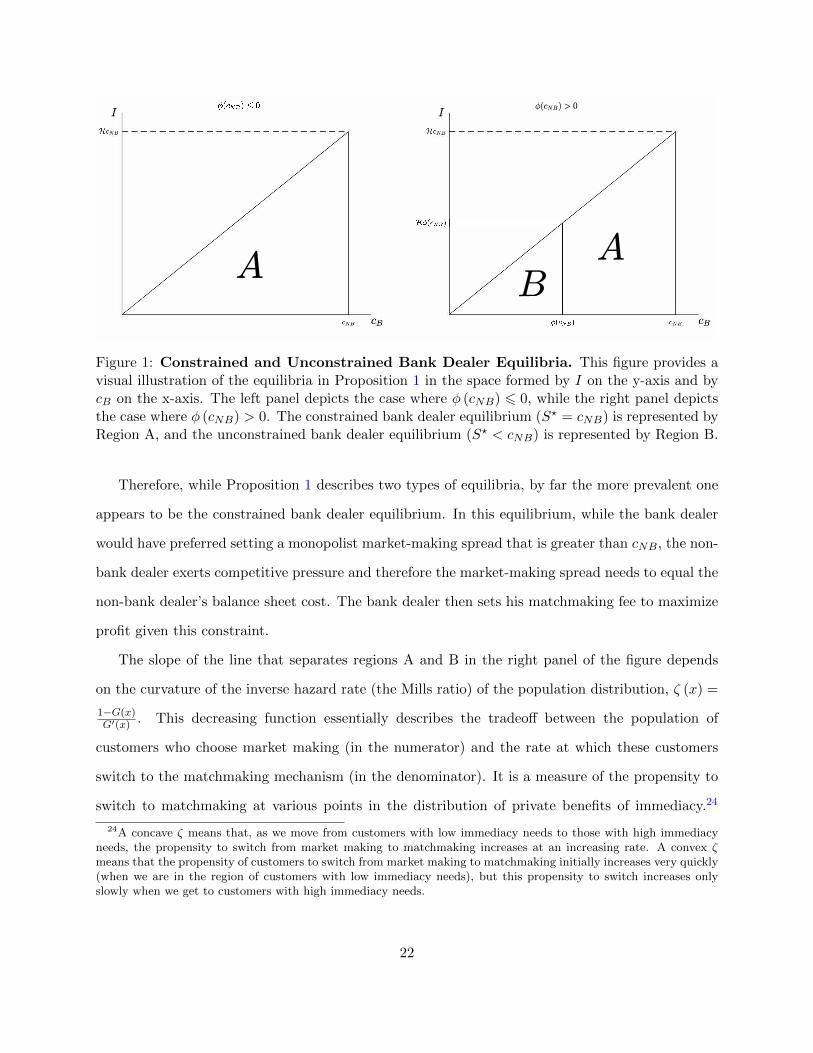
The proofs of all propositions are provided in the Appendix. Figure 1 provides a graphical
illustration of the equilibria described in Proposition 1 in the space formed by I on the y-axis and
by cB on the x-axis. The left panel of the figure shows that when φ (cNB) 6 0, only the constrained
equilibrium exists for the entire range of cB ≤ cNB. The right panel shows that when φ (cNB) > 0,
constrained equilibria in region A exist for any level of the matchmaking cost (provided that the
balance sheet cost is above a certain level). The unconstrained bank dealer equilibrium (region B)
exists only if both the matchmaking cost and the bank dealer’s balance sheet cost are low.23
23For example, if the need for immediacy of customers is exponentially distributed, then ζ (cNB) = E (G) andφ (cNB) = cNB − E (G). The left panel then shows that whenever the balance sheet cost of the non-bank dealeris smaller than the mean value of immediacy in the population of customers, cNB ≤ E (G), only the constrainedbank dealer equilibrium exists. If cNB > E (G) and the matchmaking cost is in the range [H (cNB − E (G)) ,HcNB ],again only the constrained bank dealer equilibrium exists. If cNB > E (G) and the matchmaking cost is lower thanH (cNB − E (G)), then there are two possible cases. If the balance sheet cost of the bank dealer is above a certainthreshold, again only the constrained bank dealer equilibrium exists. Only if the balance sheet cost of the bank dealeris rather low (between I
H and cNB − E (G)) does the unconstrained bank dealer equilibrium exist.
21
I I cp(cNB) > 0
A B
A
Figure 1: Constrained and Unconstrained Bank Dealer Equilibria. This figure provides avisual illustration of the equilibria in Proposition 1 in the space formed by I on the y-axis and bycB on the x-axis. The left panel depicts the case where φ (cNB) 6 0, while the right panel depictsthe case where φ (cNB) > 0. The constrained bank dealer equilibrium (S? = cNB) is represented byRegion A, and the unconstrained bank dealer equilibrium (S? < cNB) is represented by Region B.
Therefore, while Proposition 1 describes two types of equilibria, by far the more prevalent one
appears to be the constrained bank dealer equilibrium. In this equilibrium, while the bank dealer
would have preferred setting a monopolist market-making spread that is greater than cNB, the non-
bank dealer exerts competitive pressure and therefore the market-making spread needs to equal the
non-bank dealer’s balance sheet cost. The bank dealer then sets his matchmaking fee to maximize
profit given this constraint.
The slope of the line that separates regions A and B in the right panel of the figure depends
on the curvature of the inverse hazard rate (the Mills ratio) of the population distribution, ζ (x) =
1−G(x)G′(x) . This decreasing function essentially describes the tradeoff between the population of
customers who choose market making (in the numerator) and the rate at which these customers
switch to the matchmaking mechanism (in the denominator). It is a measure of the propensity to
switch to matchmaking at various points in the distribution of private benefits of immediacy.24
24A concave ζ means that, as we move from customers with low immediacy needs to those with high immediacyneeds, the propensity to switch from market making to matchmaking increases at an increasing rate. A convex ζmeans that the propensity of customers to switch from market making to matchmaking initially increases very quickly(when we are in the region of customers with low immediacy needs), but this propensity to switch increases onlyslowly when we get to customers with high immediacy needs.
22

A convex ζ, which characterizes many popular distributions such as the normal and uniform
distributions, would result in a boundary that intersects the x-axis to the left of φ (cNB) and hence
an even larger region A of the constrained equilibrium. A concave ζ would result in a boundary
that intersects the x-axis to the right of φ (cNB), increasing the size of region B.
How does an increase in the bank dealer’s regulatory costs impact the market? We can show
that bank dealer profits are unequivocally lower when regulatory costs increase (or, put differently,
as the bank dealer’s implicit too-big-to-fail subsidy is reduced). This would explain why bank
dealers opposed post-crisis regulations that increased their balance sheet costs. Less obvious is
what happens to customer welfare and observable market outcome. To determine how an increase
in bank regulatory costs impacts these quantities as cB increases, we need to investigate how these
attributes change within each of the two equilibrium regions.
Proposition 2 provides the comparative statics for the constrained bank dealer equilibrium.
Specifically, we look at the following observable market outcomes: trading costs (market-making
spread, matchmaking fee, and average transaction costs), and customers’ choice of trading outcome
and venue (i.e., volume and the market share of the two trading mechanisms). Most importantly,
we examine how an increase in the bank dealer’s balance sheet cost impacts (the unobservable)
overall customer welfare.
Proposition 2. When cB increases in the constrained bank dealer equilibrium:
1. The spread is unchanged (S? = cNB), the matchmaking fee f? decreases, and average transaction
costs decrease.
2. Trading volume increases, matchmaking increases, and market making decreases.
3. Overall customer welfare, πc, increases.
The comparative statics in Proposition 2 are all unambiguously signed. As competition from
the non-bank dealer constrains the bank dealer’s ability to pass the rising regulatory costs on to his
market-making customers, the bank dealer seeks to extract higher profits from the matchmaking
business. To this end, he increases overall trading volume (which is equivalent in our setting to
23
increasing the fraction of customer types who trade, 1−G (f?)) by lowering the matchmaking fee
to attract customers with a low need for immediacy.
Shifting more trading to the less expensive matchmaking service lowers average transaction
costs in the market, but even more notable is that overall customer welfare increases. The welfare
gains come from three groups of customers. The first group refrains from trading when cB is
sufficiently low, but when the bank dealer lowers the matchmaking fee they begin trading and thus
contribute to overall customer welfare. The second group consists of customers who trade via the
matchmaking mechanism either way, but when cB increases their welfare goes up because they pay
a lower fee.
The third group are those customers who find it optimal to switch from market making to
matchmaking when cB increases because the matchmaking fee goes down. Given that the spread
in this equilibrium region is constrained, their expected utility from using the market-making
service does not change when cB rises. Their choice to switch means that their expected utility
considering both the lower fee and the expected waiting costs in the matchmaking service is higher
(except for the marginal customer who is indifferent between the two trading mechanisms). Hence,
all customers are either better off or no worse off as cB goes up, which means that equilibria
with higher bank regulatory costs Pareto-dominate those with lower bank regulatory costs in this
region.25
It is in the constrained equilibrium that customers derive the most benefit from increased bank
regulatory costs because the industrial organization angle (increased competition from the non-
bank dealer) interacts with the market microstructure angle (increased utilization of a lower-cost
alternative trading mechanism), leading to reduced bank dealer rents and increased overall customer
welfare. We stress that if the bank dealer had operated only a market-making business, investor
25To simplify the model, the matching rate of customers in the matchmaking mechanism is directly determined bythe bank dealer’s search technology. We believe that the increase in overall customer welfare when bank regulatorycosts go up in the constrained bank dealer equilibrium would hold in a more general search specification (e.g., Duffie,Garleanu, and Pedersen (2005)) in which the matching intensity depends on the mass of customers who choosematchmaking. Specifically, Proposition 2 shows that the market share of matchmaking monotonically increases incB . Under an alternative structure in which the size of the pool of searching customers impacts the matching rate,this increase in market share would result in a higher matchmaking speed H and make the matchmaking service evenmore beneficial to customers. In this case, the switch to matchmaking would likely be more pronounced as cB goesup, further improving overall customer welfare.
24

welfare would not have increased in this equilibrium. The change in equilibrium market structure
is therefore at the core of the result that overall customer welfare increases.
While we can see from Proposition 1 that the constrained equilibrium is more prevalent in that
it exists for the entire range of search costs (0,Hφ (cNB)) and irrespective of whether φ (cNB) is
negative or positive, the unconstrained bank dealer equilibrium prevails if both the search cost
and the balance sheet cost of the bank dealer are very low. The next proposition shows that the
manner in which increased regulatory costs impacts customers and market outcomes in this region
can differ considerably.
Proposition 3. When cB increases in the unconstrained bank dealer equilibrium:
1. The spread S? increases, the matchmaking fee f? is unchanged, and average transaction costs
increase if cB < (1−H) f? + I and decrease if cB > (1−H) f? + I.
2. Trading volume is unchanged, matchmaking increases, and market making decreases.
3. Overall customer welfare, πc, decreases.
Why are customers worse off in the unconstrained equilibrium? The bank dealer is a monopolist
in both the market-making and matchmaking businesses. He passes any increase in regulatory costs
to the market-making customers by increasing the spread, leaving his profit per trade in this trading
mechanism unchanged. Given a particular distribution of customers’ private value (or patience),
a higher matchmaking fee increases compensation from each trade while decreasing the number
of customers who choose to trade. This tradeoff results in a unique fee that maximizes the bank
dealer’s expected profit from matchmaking that depends only on the distribution of private values
(and hence does not change as bank regulatory costs increase). As cB increases, some customers
stop paying the spread and opt instead to use the matchmaking mechanism, but the population
of customers who refrain from trading (which depends on the magnitude of the matchmaking fee)
does not change and hence volume is unchanged.
Average transaction costs can be computed as the weighted average of the market-making
spread and the matchmaking fee with the respective populations of the trading customers in each
of these mechanisms as weights. When regulatory costs increase, the spread increases but the
25

fraction of customers choosing the market-making mechanism declines, and hence the direction of
the change in average transaction costs can go either way. If the cost of balance sheet financing
is lower than the bank dealer’s matchmaking costs (the out-of-pocket search cost as well as the
expected waiting cost to receive the fee), increasing the balance sheet cost will result in higher
average transaction costs. Whether average transaction costs reach an interior maximum and begin
declining before the unconstrained equilibrium changes to the constrained equilibrium depends on
the specific distribution of customers’ private values.
Irrespective of what happens to average transaction costs, however, overall customer welfare
unequivocally decreases in the unconstrained equilibrium. This result is important in that it serves
to demonstrate that the welfare of customers is not equivalent to measures that can be estimated
from executed trades. All trading customers are worse off in this equilibrium when cB increases,
either because they pay a higher spread or because they are priced-out of the market-making
service and they incur waiting costs when utilizing the matchmaking service. Furthermore, the
population of customers who refrain from trading remains the same (because the matchmaking fee
is unchanged), and hence overall customer welfare is lower when bank regulatory costs increase.
The unconstrained bank dealer equilibrium fits with views expressed by some market participants
according to which a higher bank dealer balance sheet cost would negatively impact market liquidity
and customer welfare. We stress that, in our model, these results arise because the bank dealer
has an unconstrained monopoly on the provision of immediacy. In addition, the existence of this
equilibrium critically depends on there being both a rather large too-big-to-fail subsidy (low cB) and
a rather low search cost in the matchmaking business. Considering the entire structure of equilibria
when cB ≤ cNB, though, a key insight that arises from our model is that counteracting the too-
big-to-fail subsidy by increasing bank regulatory costs is not welfare-improving without market
discipline. Namely, competition from non-bank dealers who stand ready to offer market-making
services is crucial to attaining the welfare-improvement result.
26

4.1.2 When cB > cNB
If regulatory costs were to further increase, the bank dealer’s balance sheet cost could potentially
exceed the non-bank dealer’s balance sheet cost, cNB. In such a case, the bank dealer would not
provide market-making services because the non-bank dealer could always charge SNB = cB − ε
and attract all customers who are willing to pay the spread to trade immediately. When cB = cNB,
the only equilibrium spread possible is S = cB = cNB and both bank and non-bank dealers make
zero profits from market making. We include this boundary point as part of Proposition 1, but it
can be added as easily to the case of cB > cNB or we could also assume that customers who would
like to use the market-making mechanism randomize between the bank and non-bank dealers.
Given that Bessembinder, Jacobsen, Maxwell, and Venkataraman (2018) estimate bank dealers
handle about 87% of principal trading even after the post-crisis regulatory reform, why should we
care about the case of cB > cNB? The reason is that the same paper also presents evidence that
non-bank dealers increased their market share in principal trading from about 3% in the pre-crisis
period to about 13% in the post-regulatory-reform period. Our model is simplified in that we have
a bang-bang solution: either the bank dealer or the non-bank dealer captures all market-making
clients. The increase in principal trading by non-bank dealers documented by Bessembinder et al.
may suggest that we are getting closer to the point where cB = cNB. It is therefore important to
investigate what would happen to overall customer welfare if bank regulatory costs were to increase
past this point.
As before, we focus only on equilibria in which the bank dealer engages in matchmaking.
Specifically, given the bank dealer’s choice of f , the non-bank dealer’s problem is
πNB (cB) = maxcNB≤S≤cB
ΠNB (S) =2µ
r[(S − cNB) (1−G (b))] .
Here, we impose a tie-breaking rule according to which the bank dealer does not offer the market-
making service if its profit would be zero. This implies that, when SNB = cB, the bank dealer does
not operate the market-making business.
27

Given the non-bank dealer’s choice of S, the bank dealer’s problem is
πB (cB) = max0≤f≤S
ΠB (f) =2µ
r(Hf − I) (G (b)−G (f)) ,
where b = S−Hf1−H . The following proposition establishes the existence of an equilibrium when the
balance sheet cost of the bank dealer exceeds that of the non-bank dealer.
Proposition 4. When cB > cNB and I < Hmin{cB, cB}, there exists a unique equilibrium
such that the non-bank dealer operates the market-making service and the bank dealer operates the
matchmaking service, with cB as the unique solution of
ξ (cB)− cB − cNB1−H
= 0,
provided that G is concave or G is convex with G′′′ < 0 and H < 12 . In particular, there exists
c2 > max{cNB, IH} such that,
1. If cB ∈ (cNB, c2], the equilibrium is a constrained non-bank dealer equilibrium with S? =
cB.
2. If cB ∈ (c2,∞), the equilibrium is an unconstrained non-bank dealer equilibrium with
S? < cB.
As before, all equilibria with bank dealer matchmaking require that the search cost is not overly
high. In addition, the conditions on the curvature of the function G are required because under these
conditions the bank dealer’s best response is always continuous and unique, which can guarantee
the existence of equilibrium. When cB just exceeds cNB, we enter the constrained non-bank dealer
equilibrium region in which the non-bank dealer’s spread, SNB, is equal to the bank dealer’s balance
sheet cost, cB. As cB rises, the competitive pressure from the bank dealer eases, and the non-bank
dealer can increase his market-making spread to extract more rents. Beyond a certain point, the
bank dealer no longer exerts any competitive pressure and we reach an unconstrained non-bank
dealer equilibrium, where SNB is the non-bank dealer’s monopoly spread. In the unconstrained
28

equilibrium, further increases in the bank dealer’s balance sheet cost no longer affect the equilibrium
outcomes.
The unconstrained non-bank dealer equilibrium appears somewhat extreme and hence of limited
interest. The constrained non-bank dealer equilibrium, on the other hand, can help us answer the
question what happens to customer welfare and market outcomes when the balance sheet cost of
the bank dealer just passes that of the non-bank dealer.
Proposition 5. When cB increases in the constrained non-bank dealer equilibrium:
1. S? = cB increases, f? increases, and the change in average transaction costs is ambiguous.
2. Trading volume decreases, market making decreases, and the change in matchmaking is ambiguous.
3. Overall customer welfare, πc, decreases.
Increasing regulatory costs past the point at which the bank dealer’s balance sheet cost is
equal to cNB weakens rather than strengthens competition. The non-bank dealer increases his
spread, creating an opportunity for the bank dealer to increase his matchmaking fee as well. As
a result, more customers forgo trading and hence trading volume decreases. Most importantly,
overall customer welfare declines. The decline in welfare stems from the increase in market-making
spread and matchmaking fee for those customers who trade as well as the increase in the number
of customers who choose to refrain from trading because of the higher costs. At the same time, we
can show that both dealers’ profits go up unambiguously when bank regulatory costs increase as
each dealer specializes in a different business and is able to use his market power to extract higher
rents (the non-bank dealer from market making and the bank dealer from matchmaking).
This equilibrium demonstrates the peril of raising bank regulatory costs too much. While
customers benefit when the increase in regulatory costs counters the too-big-to-fail subsidy and
enhances competition, they fare worse if these costs are set so high that they push the bank dealer
out of the market-making business.
29

4.2 What Happens when the Cost of Matchmaking Declines?
In this section we focus on the second important development of the past decade in the corporate
bond market: technological advances that reduced the cost of matchmaking and therefore rendered
the matchmaking mechanism more attractive.26 This development is represented in our model by
a reduction in the cost of search (or effort) required to effect a transaction in the matchmaking
mechanism, I. The following proposition shows that, when competition between the bank and
non-bank dealer constrains their strategies, a lower search cost unambiguously benefits customers.
Proposition 6. When I decreases in either the constrained bank dealer equilibrium (section
4.1.1) or the constrained non-bank dealer equilibrium (section 4.1.2):
1. S? is unchanged, f? decreases, and average transaction costs decrease.
2. Trading volume increases, matchmaking increases, and market making decreases.
3. Overall customer welfare, πc, increases.
A lower matchmaking cost incentivizes the bank dealer to decrease the matchmaking fee to
attract more customers to this trading mechanism. Competition between the bank and non-bank
dealers in market-making services exerts enough pressure on the spread to essentially fix it to
equal the higher of the two balance sheet costs irrespective of changes in the matchmaking cost.
This leads to an unambiguous improvement in the welfare of customers who use the matchmaking
mechanism, including those who optimally choose to switch from market making to matchmaking
and those who start trading only after I declines. Higher volume in the matchmaking service also
benefits the bank dealer, whose profits rise alongside the increase in overall customer welfare.27
The key to this unambiguous improvement in overall customer welfare, however, is binding
competition in market-making services. We can clearly see the importance of competition by
26The report on electronic trading in fixed income markets issued by the Markets Committee of the Bank forInternational Settlements notes that growth in electronic trading has occurred primarily in the dealer-client segment,with technological innovations giving rise to new trading venues and protocols (BIS Markets Committee (2016)).Many of the systems in this segment are single-dealer platforms that are typically based on permutations of therequest-for-quote (RFQ) protocol.
27Profits of the non-bank dealer, on the other hand, decline. As the bank dealer lowers the matchmaking fee,customers switch from market making to matchmaking, leaving the non-bank dealer with a smaller market share andhence lower profits.
30

comparing these results to the comparative statics obtained in the unconstrained bank dealer
equilibrium in which the bank dealer operates as a monopolist in both trading mechanisms.
Proposition 7. When I decreases in the unconstrained bank dealer equilibrium (section 4.1.1):
1. S? increases (decreases) if ζ is convex (concave), f? decreases, and the change in average
transaction costs is ambiguous.
2. Trading volume increases, matchmaking increases, and market making decreases.
3. The change in overall customer welfare, πc, is ambiguous if ζ is convex, but is positive if ζ is
concave.
While we can show that the bank dealer’s profits unambiguously rise, the same cannot be said
about overall customer welfare. We discussed the curvature of the Mills ratio, ζ, in Section 4.1.1,
where it mattered for the shape of the boundary between regions A and B in Figure 1. Many
familiar distributions (e.g., normal, uniform) have a convex ζ, although one could easily construct
or specify distributions for which ζ is concave. Still, given the prevalence of distributions with
convex ζ, it is important to note that for such distributions the change in overall customer welfare
is ambiguous.
The reason for this ambiguity is that the monopolist bank dealer looks to increase profit margins
from the market-making business by raising the spread. Customers with high immediacy needs
who utilize the market-making mechanism are then worse off to a degree that can overwhelm
improvements for customers who place a low value on immediacy. The surplus generated by a
lower search cost in such a case can go mainly to the bank dealer, not to the customers. To
ensure that customers unequivocally benefit from technological advances that lower search costs,
one needs to be in the constrained equilibrium, which means that regulators need to increase the
balance sheet cost of the bank dealer from the very low level that enables the unconstrained bank
dealer equilibrium to prevail.
31

5 Did Post-Crisis Bank Regulations Harm Investors in the Corporate
Bond Market?
We can use the model’s insights to evaluate whether bank regulations following the financial crisis
lowered overall investor welfare. Given the wide availability of empirical evidence regarding the
US corporate bond market, we focus our discussion on this market, but the model’s insights would
apply to other markets that were similarly affected by post-crisis bank regulations. As we stress
in the introduction, empirical estimates of transaction-based measures of liquidity cannot capture
investors’ loss of welfare when finding a trading counterparty takes more time or when investors
forgo trading altogether. In contrast, our theoretical model takes these potential welfare losses into
account alongside the out-of-pocket cost of trading. Our analysis shows that the implications of
bank regulations for overall customer welfare depend on the manner in which competition between
the bank and non-bank dealers shapes the equilibrium. Hence, to evaluate the impact of post-crisis
regulations on welfare we need to tie the equilibrium regions in our model to the state of affairs
in the corporate bond market around the enactment of the bank regulations. In this section we
attempt to do so by mapping the implications of our model for observable market outcomes onto
the findings reported in the empirical literature.
The first set of results involves the somewhat surprising empirical finding that average transaction
costs have declined (Mizrach (2015), Adrian, Fleming, Shachar, and Vogt (2017), Anderson and
Stulz (2017)) or have not changed (Bessembinder, Jacobsen, Maxwell, and Venkataraman (2018),
Trebbi and Xiao (2019)) following the enactment of post-crisis regulations. In our model, the most
prevalent equilibrium is the constrained bank dealer equilibrium in which average transaction costs
unequivocally go down as cB increases (region A in Figure 1). Still, if both the matchmaking cost
and the bank dealer’s balance sheet cost are low enough, the decline in average transaction costs
could possibly start already in the right portion of the unconstrained bank equilibrium (region B
in Figure 1).28 Hence, the observation of declining average transaction costs is consistent with an
increase in the balance sheet cost of the bank dealer starting from the right portion of region B
28This would happen if cB increases beyond (1−H) f? + I before the equilibrium changes to the constrained bankequilibrium.
32

and across region A.
The second set of empirical results is that the cost of immediacy, or the cost of trading via
the market-making mechanism, has risen (Bao, O’Hara, and Zhou (2018), Dick-Nielsen and Rossi
(2018), Choi and Huh (2017)). In our model, this is also consistent with a movement that starts
in region B and ends up in region A, although it could also be consistent with an increase in
cB that potentially overshoots and exceeds the balance sheet cost of the non-bank dealer in the
constrained non-bank dealer equilibrium. The third set of empirical findings document an increase
in matchmaking volume driven by bank dealers (Bao, O’Hara, and Zhou (2018), Choi and Huh
(2017), Schultz (2017)) and a significant decline in capital commitment to market making by
bank dealers without a sufficiently large offsetting increase in market making by non-bank dealers
(Bao, O’Hara, and Zhou (2018), Bessembinder, Jacobsen, Maxwell, and Venkataraman (2018)).
In our model, such a pattern can be observed throughout the constrained and unconstrained
bank equilibria (regions A and B). This is not the pattern in the unconstrained non-bank dealer
equilibrium, however, which suggests that it is unlikely that post-crisis regulations left us in the
region where cB > cNB.
In the model, there is a clear distinction between the constrained bank equilibrium, where
the bank dealer captures the entire market-making business, and the unconstrained non-bank
equilibrium, where the non-bank dealer accommodates all customers who demand immediacy.
We would expect a more gradual transition in reality. The empirical evidence of an increase
(decline) in market-making activity by non-bank (bank) dealers following the enactment of post-
crisis regulations suggests an increase in regulatory costs across region A that left us currently
somewhere in the right portion of this region. However, the empirical evidence reported in Bessembinder,
Jacobsen, Maxwell, and Venkataraman (2018), which shows that bank dealers completely dominate
principal trading even after the post-crisis regulatory reform (with 87% of principal trading versus
13% of the non-bank dealers), suggests to us that cB is still currently below cNB.
The last set of empirical results concerns trading volume, and here we note that the findings
appear to be somewhat nuanced. Overall trading volume in bonds has significantly increased, while
turnover in each particular bond issue appears to have declined (increased) in more (less) active
33

bonds (BIS Committee on the Global Financial System (2014), Mizrach (2015), Adrian, Fleming,
Shachar, and Vogt (2017)). Turnover is computed as dollar trading volume divided by the value of
the bond issue and is used by some market participants as yet another measure of volume alongside
dollar trading volume. Given that volume is normalized by the size of the issue, though, patterns
in issuance affect this measure. Some market observers note that the low interest-rate environment
greatly boosted the attractiveness of bond financing, and business enterprises responded by issuing
a record number of bonds. According to this explanation, abnormal issuance, not a decline in the
desire to trade, reduced turnover in some bond issues (BIS Committee on the Global Financial
System (2014)). In other words, the higher observed overall dollar volume could be driven by lower
average transaction costs that attract more customers to trade bonds (as in our model), but the
record number of new issues means that some bond issues would be traded less often. The only
equilibrium region in our model in which dollar volume increases as it has in the empirical work
is the constrained bank dealer equilibrium, suggesting again an increase in the balance sheet cost
across region A.
Summarizing our discussion, the four sets of empirical findings associated with the implementation
of bank regulations in the aftermath of the financial crisis all point to the particular role that the
constrained bank dealer equilibrium plays in our model. It is reasonable to conjecture that we
were in the unconstrained bank dealer equilibrium (region B) in the pre-crisis period and ended
up in the constrained bank dealer equilibrium after bank regulations were imposed. The decline
in average transaction costs and simultaneous increase in volume suggests that we have probably
moved across a large portion of the cB range in the constrained bank equilibrium getting closer to
the point at which cB = cNB. With this in mind, we can now consider our model’s predictions for
overall customer welfare.
As Proposition 2 shows, overall customer welfare unequivocally increases as the balance sheet
cost of the bank dealer increases throughout the constrained bank dealer equilibrium in region A.
The clear mapping of the empirical findings to an increase in regulatory costs across region A in the
model coupled with our welfare implications indicate that investors in the corporate bond market
are likely better off under the current bank regulatory regime compared with the one that prevailed
34

before the financial crisis. We cannot say whether a particular feature of the Basel framework is
responsible for this result and our results do not imply that the Volcker Rule improved liquidity.
Rather, considering the empirical findings pertaining to the impact of the entire suite of post-crisis
regulations, our model would suggest that the increase in market-making costs benefits corporate
bond investors even during normal times. We believe that this insight is an important contribution
of our work to the debate over the merits of bank regulations that were imposed in the aftermath
of the financial crisis.
Lastly, our observation that post-crisis bank regulations likely caused a shift from an equilibrium
in region B to an equilibrium in region A is also important when considering technological innovations
that decrease search costs in the matchmaking business. In our model, the bank dealer earns higher
profits by adopting innovations that lower search costs in either equilibrium region. However, the
impact of such innovations on overall customer welfare is ambiguous in region B, while Proposition
6 demonstrates that overall customer welfare unambiguously increases when search costs decline
in region A. In the equilibrium that we believe is most likely prevailing in the market today,
therefore, the surplus from lower search costs is shared by both customers and bank dealers. As
such, regulations that help facilitate (or remove obstacles that could hamper) the adoption of such
innovations by bank dealers would make investors in the corporate bond market better off.
6 Robustness
In this section, we study the robustness of our main results. Section 6.1 presents a variant of the
model in which multiple differentiated bank dealers compete. Section 6.2 examines an alternative
measure of welfare.
6.1 An Oligopoly Model of Bank Dealers
Our baseline model has a single representative bank dealer. To some readers, this monopoly setting
may appear stark. In this section, we study an oligopoly model in which multiple differentiated
bank dealers compete for customers. We show that, as in the representative bank dealer model,
there is a parameter region in which overall customer welfare increases in the bank dealers’ balance
35

sheet cost. We further show that this region would shrink to zero only if bank dealers were perfectly
competitive (i.e., completely undifferentiated). Thus, as long as bank dealers have even a small
amount of market power, our main result—raising the balance sheet cost of bank dealers can
increase overall customer welfare—is robust.
Model setup
There are N + 1 dealers, consisting of N bank dealers and one non-bank dealer. The N bank
dealers, indexed by j, have identical balance sheet cost cB, search cost I, and matchmaking speed
H. The non-bank dealer has balance sheet cost cNB. Because the most empirically relevant case is
when the bank dealers have a balance sheet cost advantage over the non-bank dealer, we focus in
this section on the parameter region cB ≤ cNB.
There is a static mass 2Nµr of customers, indexed by i, and customer i has a “taste” εij ∼ F (σ)
for being a customer of bank j. The taste εij can be interpreted as customer i’s private value for
using bank j. Customers have zero taste for the non-bank dealer. The customer taste shocks εij
generate differentiation among bank dealers, which limits customer substitution and allows bank
dealers to charge positive markups. The variance of the taste shocks, σ, captures the degree of
differentiation and therefore competition between bank dealers. If taste shocks have a low variance,
bank dealers are more homogeneous, customers’ choice between them is primarily determined by
their prices, and bank dealers compete intensely by choosing lower market-making spreads and
matchmaking fees. If, on the other hand, taste shocks have a large variance, bank dealers are
more differentiated, customers put less weight on prices, and bank dealers compete less intensely
by choosing higher S and f . Our use of the variance of the taste shocks to model the degree of
differentiation and competition follows from Perloff and Salop (1985).
The timing of the model is as follows:
Stage 1. Each bank dealer j chooses (fj , Sj), and the non-bank dealer chooses SNB, all simultaneously.
Stage 2. Each customer i receives the εij taste shock and chooses to affiliate with bank dealer j. Once
affiliated, the customer can use only the services (matchmaking or market making) of bank
dealer j.
36
Stage 3. Each customer i observes her private benefit for trading immediately, x ∼ G, and chooses
between:
(a) using bank dealer j’s matchmaking service with the fee fj ,
(b) using bank dealer j’s market-making service with the spread Sj ,
(c) using the non-bank dealer’s market-making service with the spread SNB, and
(d) not trading.
In this setup, customers can substitute between market making, matchmaking, and not trading
in stage 3, and substitute between bank dealers in stage 2. The customer’s choice set in stage 3 is
identical to that in the baseline model, and the customer’s choice between multiple bank dealers
in stage 2 can be viewed as an “overlay” stage of the game whose outcome is taken as given in our
baseline model. As a result, if we take the limit as the variance of the taste shocks goes to infinity,
we effectively recover our baseline monopolist bank dealer model. On the other hand, if we take
the limit as the variance of the taste shocks goes to zero we end up in an economy in which bank
dealers are homogeneous and therefore engage in a Bertrand competition. Varying the variance of
the taste shocks, therefore, enables us to examine how the degree of market power bank dealers
wield influences our conclusions.29
Customers’ decisions
As usual, we use backward induction to solve this model. In stage 3, customer i is already locked
in to a single bank dealer. Facing (fj , Sj , SNB), customer i’s decision is the same as that of the
customer in our baseline model.
In stage 2, before observing her private value for trading, customer i’s expected utility from
29This particular oligopoly setup achieves consistency with the baseline model and at the same time builds inthe customer’s choice between bank dealers in a tractable framework. For this reason, although the setup rulesout substitution between bank dealers after the customers observe their private values, we view it as a reasonablecompromise.
37
affiliating with bank dealer j is
πcji(Sj , fj) =
∫ b
x=f(x− fj)HdG(x) +
∫ ∞x=b
(x− Sj)dG(x)︸ ︷︷ ︸πcj(Sj ,fj)
+εij , (11)
where b =Sj−Hfj
1−H , and we have labeled the portion of utility not related to taste as πcj(Sj , fj).
The customer’s decision problem in stage 2 is therefore
maxjπci(Sj , fj). (12)
For tractability, we assume that {εij} are independent and identically distributed logistic
random variables with variance π2
6 σ2. This parametrization implies that the share of customers
who choose bank j is
sj(Sj , fj , S−j , f−j) =exp( 1
σ πcj(Sj , fj))∑j′ exp( 1
σ πcj′(Sj′ , fj′)), (13)
where S−j = (Sj′)j′ 6=j and f−j = (fj′)j′ 6=j are the other bank dealers’ prices.
Bank dealers’ decisions
In stage 1, each bank dealer sets prices to maximize his profits. The bank dealer’s expected per-
capita profits is
πj = (Hfj − I)(G(b)−G(fj)) + (Sj − cB)(1−G(b)). (14)
Then, bank dealer j’s problem is
max0≤fj≤Sj≤cNB
Πj ≡2Nµ
r× sj(Sj , fj , S−j , f−j)× πj . (15)
We focus on symmetric strategies, that is, for all j and j′, we have (fj , Sj) = (fj′ , Sj′). Assuming
that such a symmetric equilibrium exists, each bank dealer’s market share would be sj = 1/N .
38

Taking the first-order condition of Πj and substituting in sj = 1/N , we obtain
∂Πj
∂fj=
2Nµ
r
[N − 1
N2
1
σ
∂πcj∂fj
πj +1
N
∂πj∂fj
]=
2µ
r
[N − 1
N
1
σ
∂πcj∂fj
πj +∂πj∂fj
], (16)
∂Πj
∂Sj=
2Nµ
r
[N − 1
N2
1
σ
∂πcj∂Sj
πj +1
N
∂πj∂Sj
]=
2µ
r
[N − 1
N
1
σ
∂πcj∂Sj
πj +∂πj∂Sj
]. (17)
From this expression, it is clear that, as σ →∞, the two partial derivatives converge to 2µr∂πj∂fj
and 2µr∂πj∂fj
, respectively, which are the same as the first-order conditions in the baseline model.
Therefore, if bank dealers are sufficiently differentiated, they will have a stable set of customers
based on taste and would no longer compete for market share.
Proposition 8. As σ → ∞, the equilibrium spread and fee charged by each bank dealer converge
to those in the baseline model.
On the other hand, as σ → 0, bank dealers are no longer differentiated and can attract customers
only by offering low prices. The following proposition shows that raising the balance sheet cost of
perfectly competitive bank dealers always decreases overall customer welfare.
Proposition 9. As σ → 0, in the limiting symmetric equilibrium, bank dealers earn zero profits,
and increasing cB results in lower overall customer welfare.
These two limiting cases illustrate the flexibility of this oligopoly model: it spans the monopoly
case at one extreme and the competitive case at the other. While the two limiting cases are relatively
simple, the generic solution for any positive but finite σ is involved. We therefore resort to numerical
solutions, and demonstrate the most salient result in Figure 2. Bessembinder, Jacobsen, Maxwell,
and Venkataraman (2018) report that “The number of dealers that comprise 70% of market share
each year ranges between 10 and 12.” Given that trading in corporate bonds is concentrated among
a small number of very large bank dealers, we use N = 10 for the number of bank dealers in our
example. Case I, Case II, and Case III in the figure represent combinations of I, H, and cNB that
correspond to Part 1, Part 2(a), and Part 2(b) of Proposition 1.
Our main result in the baseline model is that there is a region over which raising the balance
sheet cost of the bank dealer increases overall customer welfare. Our goal in this robustness section
39

is to demonstrate how the size of this region changes with the degree of market power. Therefore,
Figure 2 showcases cB on the y-axis and σ on the x-axis, with market power increasing as we move
to the right. For each σ, the lighter orange area represents the range of cB for which customer
welfare is increasing in cB, and the darker blue area represents the range for which welfare is
decreasing in cB.
A salient theme across all three cases is that, as long as there is some degree of differentiation
between banks (i.e., a modest positive σ), overall customer welfare increases in cB in a nontrivial
range of the parameter. Equally interestingly, this region seems to expand rapidly as σ increases.
Only if σ = 0 does customer welfare always decrease in cB. While we have not been able to derive
the analytical characterizations for these regions, the numerical solutions nonetheless show that
our main result—overall customer welfare increasing in the bank dealers’ balance sheet cost—is not
an artifact of the baseline monopoly model. This insight is rather robust as long as bank dealers
possess any positive amount of market power.
0 20 40 60 80 100 (bps)
1
2
3
4
5
6
7
8
9
c B (b
ps)
Case I
0 20 40 60 80 100 (bps)
2
4
6
8
10
12
c B (b
ps)
Case II
Customer welfare non-increasing in cB Customer welfare increasing in cB
0 20 40 60 80 100 (bps)
6
7
8
9
10
11
12
13
14
15c B
(bps
)Case III
Figure 2: Regions of (σ, cB) in which overall customer welfare increases or decreasesin cB. In all three cases, N = 10, H = 0.5, and we use the exponential distribution for G, withE(G) = 10 bps. In Case I, cNB = 9 bps and I = 0.5 bp. In Case II, cNB = 12 bps and I = 0.5 bp.In Case III, cNB = 15 bps and I = 3.
40

6.2 An Alternative Welfare Measure
Throughout the paper we focus on customer welfare as the metric with which to evaluate the
ultimate benefit or cost of post-crisis regulations. This quantity, defined in (5), reflects the gains
from trade of customers in the model (who represent the investor population in our economy). For
us, this is a natural benchmark for regulators to consider.
One may argue that our customer welfare measure misses two components. First, the too-big-
to-fail subsidy the bank dealer receives—reflected in the difference in balance sheet costs between
the bank and non-bank dealers—ultimately comes out of the pocket of investors (or the public in
general), so we may want to include this adjustment. Second, both the bank and non-bank dealers
are agents in the economy, and one may want to include them in the definition of welfare as well.
Therefore, we consider an alternative welfare measure as the sum of customer welfare and the
two dealers’ profits, while adjusting for the implicit too-big-to-fail subsidy of the bank dealer:
W = πc + πB + πNB −2µ
r(1−G (b)) (cNB − cB) IS=SB︸ ︷︷ ︸
Too-big-to-fail subsidy of the bank dealer, if cB < cNB
. (18)
The first three terms of this expression are defined in the model section, but the last term
requires additional discussion. Our assumption is that, without giving an implicit public subsidy to
the bank dealer, the balance sheet costs of the bank dealer would be similar to those of the non-bank
dealer—that is, the same market-making activity would require the same cost of capital regardless
of who provides it.30 Hence, the difference between the two balance sheet costs, multiplied by the
number of customers who trade using the market-making services of the bank dealer, represents
the welfare loss to investors associated with granting this subsidy to the bank dealer. As post-crisis
regulations increase the market-making costs of the bank dealer, the likelihood that the dealer
would need to be rescued decreases, and with it the implicit subsidy. As cB approaches cNB, the
subsidy given to the bank dealer’s balance sheet cost disappears. The indicator function at the
end of the term is there to ensure that the subsidy is considered only when the bank dealer makes
30The cost of capital in this context means the cost of capital of the activity, not of the entire institution that mayhave many subsidiaries. In the data, the cost of capital for each business line might be difficult to observe.
41

markets.
Because the subsidy to the bank dealer is relevant if and only if the bank dealer makes markets,
we can make the intuition in (18) more transparent by expanding it in the region cB < cNB (hence
πNB = 0):
W =2µ
r
[∫ b
x=f(Hx− I)dG(x) +
∫ ∞x=b
(x− cNB)dG(x)
], if cB < cNB. (19)
This expression essentially measures investors’ gains from trades, after adjusting for the search
cost I and the non-bank dealer’s balance sheet cost cNB, which is taken to be the market-determined,
risk-based balance sheet cost of market-making activity. While cB does not show up explicitly in
(19), an increase in cB changes the equilibrium values of f , b, and H. Overall, W reflects the
allocative efficiency of the market. Its comparative statics with respect to cB are shown in the
following proposition.
Proposition 10. In the equilibrium of Proposition 1, the welfare measure W is increasing in cB.
Proposition 10 shows that, once the subsidy of the bank dealer is explicitly accounted for,
market-wide welfare increases in the balance sheet cost of the bank dealer. While this result is
unambiguous, there are good reasons to focus on overall customer welfare, πc, rather than on W .
In particular, the dealers’ profits πB and πNB arise from their market power, and it is hard to
imagine a situation in which regulators justify their actions by appealing to the need to maximize
banks’ market power rents. As such, we think that overall customer welfare remains the most
natural metric in our framework with which to judge the impact of post-crisis regulations on the
corporate bond market.
7 Concluding Remarks
Our paper highlights the complex and multifaceted consequences that post-crisis bank regulations
have for market liquidity and investor welfare. While the explicit goal of those regulations was to
enhance financial stability in times of stress, our work shows that these regulations can improve
market efficiency even during normal times by prompting a change in the nature of liquidity
provision. In particular, post-crisis regulations eliminate obstacles to competition in the most
42

profitable business (market making) and incentivize bank dealers to reprice their services to attract
customers to an alternative market structure (matchmaking) that is better at serving the needs of
many customers. The industrial organization angle combines with the market microstructure angle
to deliver this positive outcome.
The key insight we offer in this paper is that an increase in regulatory costs imposed on banks can
make customers in the corporate bond market better off. Specifically, our focus is on balance sheet
costs that were imposed on banks following the financial crisis to deter proprietary trading and as
a result increased the costs of market making. A notable aspect of our work is that we do not focus
on whether these costs reduce the likelihood or severity of a crisis, which are presumably the stated
goals of the regulation. Rather, we show that the increase in regulatory costs can lower average
transaction costs during normal times and, more importantly, increase overall customer welfare.
The driving forces behind our results are three elements that characterize the corporate bond
market: the coexistence of two distinct trading mechanisms (market making and matchmaking),
the market power enjoyed by bank dealers, and potential market-making competition from non-
bank dealers. Although our paper is motivated by and specifically addresses observations in the
corporate bond market, the model we present can be applied to other over-the-counter markets
that feature these three elements.
How can customers be made better off by regulations that deter market making? The rationale
is that while market making is a very profitable form of intermediation for bank dealers, it can be
an expensive form of intermediation for customers. When regulation increases the cost of market
making for bank dealers and competition prevents them from transferring the cost increase to their
customers, bank dealers are incentivized to lower fees in their matchmaking business in order to
raise the volume of trading. This increases overall customer welfare because more customers can
now be better served by a menu of trading mechanisms that cater to their needs. If market making
were the only trading mechanism, raising regulatory costs would not have made customers better
off. The change in equilibrium market structure is integral to the result that overall customer
welfare increases. The welfare gains are even more pronounced when combined with the second
important development of the past decade: technological advances that reduce search costs in the
43

matchmaking mechanism.
Regulators always worry about the unintended consequences of their regulatory interventions.
While increasing the costs of market making was meant to enhance bank dealers’ resilience in times
of market stress, we believe that one (perhaps) “unintended” benefit of these bank regulations was to
push bank dealers to enhance their matchmaking service. This can improve overall customer welfare
during normal times and therefore materially changes the supposed tradeoff between resilience in
times of stress and day-to-day liquidity. The market microstructure angle in this case is crucial to
delivering this result. It is also important to emphasize that the improvement in customer welfare
in our model likely understates the extent of the true effect. Our model intentionally shuts off
one of the routes through which customers are made better off when they switch to matchmaking.
Specifically, the rate at which customers are matched in a more general search model could rise
as more customers switch to trading through the matchmaking mechanism, reducing waiting costs
and further enhancing overall customer welfare.
Raising regulatory costs beyond a certain level would inevitably worsen welfare. A natural
question is whether we can help regulators identify the optimal level of such costs. We show
that overall customer welfare increases as the cost differential between bank and non-bank dealers
shrinks. Bank regulators can therefore consider the market-making costs of non-bank dealers to
help them judge the level they should impose on bank dealers to ensure sufficient competition.
Five regulatory agencies—the Fed, the FDIC, the Office of the Comptroller of the Currency, the
SEC, and the CFTC—have recently adopted the revised Volcker Rule.31 The revision was intended,
among other things, to “provide banking entities with clarity about what activities are prohibited.”
While our model is not about the Volcker Rule per se, we stress that simply lowering the regulatory
costs of bank dealers need not help liquidity in the corporate bond market nor would it necessarily
improve customer welfare. Our analysis suggests that, in addition to using the market-making
costs of non-bank dealers as a benchmark, regulators could seek to incentivize greater utilization
of matchmaking to help ensure that customers continue to benefit even as bank regulatory costs
decline.
31See https://www.sec.gov/rules/final/2019/bhca-7.pdf.
44

All theoretical models employ simplifications in the process of creating the appropriate structure
and deriving the results. Our model is no different. Aiming for robustness and clarity necessitates
abstracting from some features of the economic environment. One example is that we do not
model the matchmaking business of non-bank dealers. Several other such features—intermediation
chains, dealer inventory, the nature of dealer funding, and the moral hazard problem that arises
when a customer employs an agent for searching—have recently been discussed in other papers
(An, Song, and Zhang (2017), An and Zheng (2017), Li and Li (2017), and Cimon and Garriott
(2019)). Partially for that reason we forgo incorporating them in our model (e.g., we abstract
from the inventory consideration by using the same arrival rates for buyers and sellers). Instead,
we focus on dimensions we deem critical to understanding how customer welfare in the corporate
bond market changes when regulation increases the costs of market making by bank dealers: the
dual trading mechanisms, dealer market power, and the nature of competition between bank and
non-bank dealers. The resulting model provides insights that we hope capture the more salient
trade-offs.
Crucial to our analysis are customers who optimize over several key choices—from the basic
decision of whether to trade to the tradeoff between search time and the cost of execution in
the two trading mechanisms—but we recognize that we could not capture all aspects of customer
behavior. For example, increased market-making costs could incentivize customers to shift their
trading to newly issued securities to minimize transaction costs, and such coping strategies may
limit portfolio flexibility. Similarly, customers may choose to reduce their average trade size in
response to the higher cost of market making. We believe that these aspects of customer behavior
(choosing newer issues or a smaller trade size) play a lesser role in determining customer welfare
than the pronounced shift from market making to matchmaking, but nonetheless they suggest a
complexity to the manner in which customers respond to changes in their economic environment.
The evolving regulatory frameworks and the breathtaking pace at which technology impacts
securities markets continue to dominate the agendas of regulators, practitioners, and academics.
We hope that our work would serve to both highlight important tradeoffs and spur additional work
on the changing nature of our securities markets.
45

References
Adrian, T., M. Fleming, O. Shachar, and E. Vogt. 2017. Market Liquidity After the FinancialCrisis. Annual Review of Financial Economics 9:43–83.
Allahrakha, M., J. Centina, B. Munyan, and S. Watugala. 2019. The Effects of the Volcker Ruleon Corporate Bond Trading: Evidence from the Underwriting Exemption. Working Paper.
An, Y., Y. Song, and X. Zhang. 2017. The Intermediary Rat Race. Working Paper.
An, Y., and Z. Zheng. 2017. Conflicted Immediacy Provision. Working Paper.
Anand, A., C. Jotikasthira, and K. Venkataraman. 2020. Do Buy-Side Institutions Supply Liquidityin Bond Markets? Evidence from Mutual Funds. Forthcoming, Review of Financial Studies.
Anderson, M., and R. Stulz. 2017. Is Post-Crisis Bond Liquidity Lower? Working Paper.
Bagnoli, M., and T. Bergstrom. 2005. Log-concave probability and its applications. EconomicTheory 26:445–469.
Bao, J., M. O’Hara, and X. (Alex) Zhou. 2018. The Volcker Rule and corporate bond marketmaking in times of stress. Journal of Financial Economics 130:95–113.
Bessembinder, H., S. Jacobsen, W. Maxwell, and K. Venkataraman. 2018. Capital Commitmentand Illiquidity in Corporate Bonds. Journal of Finance 73:1615–61.
BIS Committee on the Global Financial System. 2014. Market-making and proprietary trading:industry trends, drivers and policy implications. Report.
———. 2016. Fixed income market liquidity. Report.
BIS Markets Committee. 2016. Electronic trading in fixed income markets. Report.
Bulow, J., and P. Klemperer. 2002. Prices and the Winner’s Curse. The RAND Journal ofEconomics 33:1–21.
Chang, B., and S. Zhang. 2020. OTC Market Structure under Reforms. Working Paper.
Chen, Y., and M. Riordan. 2008. Price-Increasing Competition. The RAND Journal of Economics39:1042–1058.
Chernenko, S., and A. Sunderam. 2018. Corporate Bond Liquidity: A Revealed PreferenceApproach. Working Paper, Harvard Business School.
Choi, J., and Y. Huh. 2017. Customer Liquidity Provision: Implications for Corporate BondTransaction Costs. Working Paper.
Cimon, D. A., and C. Garriott. 2019. Banking Regulation and Market Making. Working Paper.
Davis Polk. 2014. Supplementary Leverage Ratio. Memo.
Dick-Nielsen, J., and M. Rossi. 2018. The Cost of Immediacy for Corporate Bonds. The Review ofFinancial Studies 32:1–41.
46
Duffie, D. 2012. Market Making Under the Proposed Volcker Rule. Working Paper.
Duffie, D. 2018. Post-Crisis Bank Regulations and Financial Market Liquidity. Baffi Lecture.
Duffie, D., N. Garleanu, and L. H. Pedersen. 2005. Over-the-Counter Markets. Econometrica73:1815–47.
Ederington, L. H., W. Guan, and P. K. Yadav. 2014. Dealer Spreads in the Corporate Bond Market:Agent vs. Market-Making Roles. Working Paper.
Goldstein, M. A., and E. S. Hotchkiss. 2020. Providing Liquidity in an Illiquid Market: DealerBehavior in U.S. Corporate Bonds. Journal of Financial Economics 135:16–40.
Greenwood, R., S. G. Hanson, J. C. Stein, and A. Sunderam. 2017. Strengthening and StreamliningBank Capital Regulation. Brookings Papers on Economic Activity.
Fudenberg, D., and J. Tirole. 1991. Game Theory. MIT Press.
Johnson, J.P., and D.P. Myatt. 2013. Multiproduct Quality Competition: Fighting Brands andProduct Line Pruning. The American Economic Review 93:748–774.
Li, J., and W. Li. 2017. Agency Trading and Principal Trading. Working Paper.
Katz. M. 1984. Firm-Specific Differentiation and Competition Among Multiproduct Firms. Journalof Business 57:149–166.
Mussa, M., and S. Rosen. 1978. Monopoly and Product Quality. Journal of Economic Theory18:301–317.
Mizrach, B. 2015. Analysis of Corporate Bond Liquidity. Working Paper.
Nocke, V., and N. Schutz. 2018. Multiproduct-Firm Oligopoly: An Aggregative Games Approach.Econometrica 86:523–557.
O’Hara, M. 1995. Market Microstructure Theory. John Wiley & Sons.
O’Hara, M., and X. (Alex) Zhou. 2020. The Electronic Evolution of Corporate Bond Dealers.Forthcoming, Journal of Financial Economics.
Perloff, J.M., and S.C. Salop. 1985. Equilibrium with product differentiation. Review of EconomicStudies 52:107-120.
Randall, O. 2015. How Do Inventory Costs Affect Dealer Behavior in the US Corporate BondMarket? Working Paper.
Schultz, P. 2001. Corporate bond trading costs: A peek behind the curtain. Journal of Finance56:677–98.
———. 2017. Inventory Management by Corporate Bond Dealers. Working Paper.
Trebbi, F., and K. Xiao. 2019. Regulation and Market Liquidity. Management Science 65:1949–1968.
Weyl, G., and M. Fabinger. 2013. Pass-Through as an Economic Tool: Principles of Incidenceunder Imperfect Competition. Journal of Political Economy 121:528–583.
47

Appendix
A List of Variables
Table 1: List of Model Variables
Variables Explanations
v Expected fundamental value of the assetr Discount rate
G(·) Cumulative distribution function of customer’s private value of tradingimmediately
µ Arrival rate of new buyers (and new sellers)
ζ(·) ζ (x) = 1−G(x)G′(x)
SB Bank dealer’s market-making spreadSNB Non-bank dealer’s market-making spreadcB Bank dealer’s balance sheet costcNB Non-bank dealer’s balance sheet costI Matchmaking costH Search intensity in the matchmaking serviceH Speed of matchmakingf Matchmaking feeb Private value of the marginal customer who is indifferent between
matchmaking and market-makingπc Overall customer welfareπB Bank dealer’s profitπNB Non-bank dealer’s profitφ(·) φ(x) = x− ζ(x)
48

B Proof of Propositions
B.1 Proof of Proposition 1
The bank dealer’s problem is
πB (cB) = max0≤f≤S≤cNB
ΠB (cB)
where
ΠB (cB) =2µ
r
[(Hf − I)
(G
(S −Hf1−H
)−G (f)
)+ (S − cB)
(1−G
(S −Hf1−H
))].
Consider the following change of variables,
b =S −Hf1−H
;
then
ΠB (cB) =2µ
r[(Hf − I) (G (b)−G (f)) + ((1−H) b+Hf − cB) (1−G (b))] , (20)
and the domain {(f, S) |0 ≤ f ≤ S ≤ cNB} becomes {(f, b) |0 ≤ f ≤ b; (1−H) b+Hf ≤ cNB}, whichis a triangle in the (f, b) space.
The first-order derivatives of (20) are
∂ΠB
∂f=
2µ
rHG′ (f)
[1−G (f)
G′ (f)− f +
I
H
],
∂ΠB
∂b=
2µ
r(1−H)G′ (b)
(1−G (b)
G′ (b)− b+
cB − I1−H
).
Since φ (x) = x − 1−G(x)G′(x) is an increasing function, ΠB (f, b) is a unimodal function of f with
maximum satisfying φ (fmax) = IH , and ΠB (f, b) is a unimodal function of b with maximum
satisfying φ (bmax) = cB−I1−H . One immediate observation is that
fmax < bmax ⇐⇒I
H<cB − I1−H
⇐⇒ cB >I
H.
When φ (cNB) ≤ 0, we must have φ (cNB) < IH , which implies fmax > cNB. Then, the
solution (f?, b?) either satisfies f? = b?, so there is no matchmaking, or satisfies the constraint(1−H) b? + Hf? = cNB. When cB > I
H , suppose the bank dealer chooses f = b = S. It isstraightforward to obtain
∂ΠB
∂(−f)|f=b=S =
2µ
r
H1−H
G′ (f)
(cB −
I
H
)> 0.
In this case, the bank dealer always has an incentive to lower the fee and therefore matchmakingmust exist. The equilibrium must satisfy (1−H) b?+Hf? = cNB, which is equivalent to S? = cNB.
49

The equilibrium fee f? is the minimal solution (by our equilibrium refinement) of
f? = arg maxf
2µ
r
[(Hf − I)
(G
(cNB −Hf
1−H
)−G (f)
)+ (cNB − cB)
(1−G
(cNB −Hf
1−H
))].
This is the constrained bank dealer equilibrium.When φ (cNB) > 0, if I
H < φ (cNB), we have fmax < cNB. When cB > IH , the optimal solution
(f?, b?) is either (fmax, bmax) or it satisfies the constraint (1−H) b?+Hf? = cNB. Define c1 as thesolution of
1−G(cNB−Hfmax
1−H
)G′(cNB−Hfmax
1−H
) − cNB −Hfmax1−H
+c1 − I1−H
= 0.
It is easy to show that c1 ∈(IH , cNB
). When cB < c1, the constraint (1−H) b + Hf ≤ cNB
is not binding, which means that (f? = fmax, b? = bmax) must be the equilibrium. This is the
unconstrained bank dealer equilibrium. When cB ≥ c1, the constraint (1−H) b + Hf ≤ cNB isbinding, which implies S? = cNB and f? is the minimal solution (by our equilibrium refinement) of
f? = arg maxf
2µ
r
[(Hf − I)
(G
(cNB −Hf
1−H
)−G (f)
)+ (cNB − cB)
(1−G
(cNB −Hf
1−H
))].
This is also the constrained bank dealer equilibrium.If IH ≥ φ (cNB), we have fmax ≥ cNB. Then, the solution (f?, b?) either satisfies f? = b?,
so there is no matchmaking or satisfies the constraint (1−H) b? + Hf? = cNB. When cB > IH ,
suppose the bank dealer chooses f = b = S. In this case, we have
∂ΠB
∂(−f)|f=b=S =
2µ
r
H1−H
G′ (f)
(cB −
I
H
)> 0,
so the bank dealer has an incentive to lower the fee and therefore matchmaking must exist and theequilibrium must be constrained, S? = cNB. The equilibrium fee f? is the minimal solution (byour equilibrium refinement) of
f? = arg maxf
2µ
r
[(Hf − I)
(G
(cNB −Hf
1−H
)−G (f)
)+ (cNB − cB)
(1−G
(cNB −Hf
1−H
))].
This is the constrained bank dealer equilibrium.From this proposition, we know that when cB ∈
(IH , cNB
], the bank dealer always operates the
matchmaking business. This implies that, if one starts with an equilibrium in which the parameterssatisfy cB ∈
(IH , cNB
), then increasing the balance sheet cost locally or decreasing the matchmaking
cost locally will still make the condition cB ∈(IH , cNB
]hold, which means that matchmaking will
exist in the new equilibrium as well. If one starts with an equilibrium in which the parameterssatisfy cB = cNB and I
H < cNB, then decreasing the matchmaking cost locally will still make thecondition cB ∈
(IH , cNB
]hold, and in the proof of Proposition 4 we will show that increasing the
balance sheet cost locally in this case will also lead to equilibrium with matchmaking.
50

B.2 Proof of Proposition 2
In this equilibrium, obviously S? = cNB is unchanged. f? is the minimal solution of the followingproblem
f? = arg maxf
2µ
r
[(Hf − I)
(G
(cNB −Hf
1−H
)−G (f)
)+ (cNB − cB)
(1−G
(cNB −Hf
1−H
))].
Since∂2[(Hf − I)
(G(cNB−Hf
1−H
)−G (f)
)+ (cNB − cB)
(1−G
(cNB−Hf
1−H
))]∂cB∂f
< 0,
by Topkis’s theorem, when cB increases, f? must decrease. Therefore, b? = cNB−Hf?1−H must increase.
Average transaction costs are
AC =(G (b?)−G (f?)) f? + (1−G (b?))S?
1−G (f?)
= S? − G (b?)−G (f?)
1−G (f?)(S? − f?) . (21)
When cB increases, we know that f? decreases and b? increases, thus
G (b?)−G (f?)
1−G (f?)=
G (b?)−G (f?)
1−G (b?) +G (b?)−G (f?)=
1
1 + 1−G(b?)G(b?)−G(f?)
increases. We also know that (S? − f?) increases, which means that AC decreases.The trading volume (1−G (f?)) must increase because f? decreases. Matchmaking (G (b?)−G (f?))
must increase because b? increases, which also implies that market making (1−G (b?)) decreases.Overall customer welfare is
πc =
∫ b?
f?H (x− f?) dG (x) +
∫ ∞b?
(x− S?) dG (x) ,
sodπcdcB
=
∫ b?
f?H−df
?
dcBdG (x) > 0.
B.3 Proof of Proposition 3
The equilibrium fee f? can be found from φ (f?) = IH , so it is independent of cB. b? is the solution
to φ (b?) = cB−I1−H , so b? is increasing in cB. Thus, S? = (1−H) b?+Hf? is increasing in cB. Average
transaction costs are
AC =(G (b?)−G (f?)) f? + (1−G (b?))S?
1−G (f?)
=(G (b?)−G (f?)) f? + (1−G (b?)) (Hf? + (1−H) b?)
1−G (f?).
51

Then,
dAC
dcB=db?
dcB· G′ (b?) f? + (−G′ (b?)) (Hf? + (1−H) b?) + (1−G (b?)) (1−H)
1−G (f?)
=db?
dcB· G′ (b?) (1−H)
1−G (f?)
(f? − b? +
1−G (b?)
G′ (b?)
)=db?
dcB· G′ (b?) (1−H)
1−G (f?)
(f? − cB − I
1−H
).
When cB < (1−H) f?+I, average transaction costs are increasing in cB; when cB ≥ (1−H) f?+I,average transaction costs are decreasing in cB.
Since f? is unchanged and b? increases, trading volume (1−G (f?)) must be unchanged.Matchmaking (G (b?)−G (f?)) increases, and market making (1−G (b?)) decreases.
Overall customer welfare is
πc =2µ
r
[∫ b?
f?H (x− f?) dG (x) +
∫ ∞b?
(x− S?) dG (x)
],
sodπcdcB
=2µ
r
∫ ∞b?−dS
?
dcBdG (x) < 0.
B.4 Proof of Proposition 4
The non-bank dealer’s profit function is
ΠNB (S) =2µ
r[(S − cNB) (1−G (b))] .
To establish the existence of an equilibrium and find the equilibrium, we first conjecture thatthe equilibrium exists, and then verify it.
Suppose the equilibrium is (f?, S?). The first observation is that, for bank dealer, f < IH is
strictly dominated by f = IH . Then, given any f ≥ I
H , let us consider the properties of the non-bankdealer’s best response function without considering the constraint S ≤ cB.
The first-order derivative of the non-bank dealer’s profit is
dπNBdS
=2µ
r
[1−G (b)− (S − cNB)G′ (b)
1
1−H
]=
2π
rG′ (b)
[1−G (b)
G′ (b)− S − cNB
1−H
].
We first verify that matchmaking services must be offered in equilibrium. To see this, if there is nomatchmaking in equilibrium, then the non-bank dealer’s best response is SBR = cB. Since in thiscase I
H < cB, the bank dealer can always choose f = cB − ε to obtain positive revenues. Thus, inequilibrium (if it exists), matchmaking services must be offered.
52

Given any f ≥ IH , we can show
1−G (b)
G′ (b)− S − cNB
1−H|S=cNB
> 0
1−G (b)
G′ (b)− S − cNB
1−H|S=∞ < 0.
It is easy to see that 1−G(b)G′(b) −
S−cNB1−H is strictly decreasing in S. Define M (S, f) =
1−G(S−Hf1−H )
G′(S−Hf1−H )
−S−cNB
1−H . Then, the best response SBR (f) is unique and is solved by
M (SBR, f) = 0.
We want to find a uniform upper bound for the non-bank dealer’s equilibrium strategy to helpus use the Kakutani Fixed-Point Theorem later. The best response is solved by
M (SBR, f) = 0⇐⇒ SBR (f)− cNB1−H
=1−G
(SBR(f)−Hf
1−H
)G′(SBR(f)−Hf
1−H
) ≤ 1−G (0)
G′ (0)
⇐⇒ SBR (f) ≤ cNB + (1−H)1−G (0)
G′ (0).
So WLOG, we just focus on the non-bank dealer’s strategy space S ∈[cNB, cNB + (1−H) 1−G(0)
G′(0)
].
Since M is continuously differentiable in both S and f , we know that the unique best responsefunction SBR (f) is also continuous. Besides,
∂M
∂SdSBR +
∂M
∂fdf = 0 =⇒ dSBR
df= −
∂M∂f
∂M∂S
.
It is obvious that∂M
∂f> 0,
∂M
∂S< 0,
so we must havedSBRdf
> 0.
Hence, SBR (f) is strictly increasing in f .Consider the bank dealer’s best response function. Given the non-bank dealer’s choice
S ∈[cNB, cNB + (1−H)
1−G (0)
G′ (0)
],
53

the first-order derivative of the bank dealer’s profit function is
r
2µ
∂πB∂f
= H (G (b)−G (f)) + (Hf − I)
(− H
1−HG′ (b)−G′ (f)
)= HG′ (f)
[1−G (f)
G′ (f)− f +
I
H
]−HG′ (b)
(Hf − I1−H
+1−G (b)
G′ (b)
)= HG′ (f)
[1−G (f)
G′ (f)− Hf − I
H
]−HG′ (b)
(1−G (b)
G′ (b)+Hf − I1−H
).
It is clear that ∂πB∂f |f= I
H> 0 and ∂πB
∂f |f=S < 0, so the best response fBR (S) must be interior. Thus,
the FOC must be satisfied and we have
1−G (fBR)
G′ (fBR)− fBR +
I
H> 0⇐⇒ φ (fBR) <
I
H.
Remember that the best response must satisfy fBR ∈[IH , cB
], so we have fBR ∈
[IH ,min{φ−1
(IH), cB}
].
In region fBR ∈[IH ,min{φ−1
(IH), cB}
]:
1. if G is concave, then G′ (f) is decreasing in f . Moreover, 1−G(f)G′(f) − f + I
H is positive and
decreasing in f , G′ (b) is increasing in f , Hf−I1−H + 1−G(b)G′(b) is increasing in f , and therefore ∂πB
∂f
is decreasing in fBR ∈[IH ,min{φ−1
(IH), cB}
]. This implies that the best response must
be unique, and we can show that the best response function is continuous by the implicitfunction theorem.
2. if G is convex, G′′′ ≤ 0 and H ≤ 12 , we can rewrite ∂πB
∂f as
r
2µ
∂πB∂f
= H (G (b)−G (f))− (Hf − I)
1−H(HG′ (b) + (1−H)G′ (f)
).
When f ≥ IH , we know H (G (b)−G (f)) is strictly decreasing in f , and (Hf−I)
1−H is positiveand strictly increasing in f . If we can show that (HG′ (b) + (1−H)G′ (f)) is increasing inf , then ∂πB
∂f would be strictly decreasing in f , implying that the the best response is unique.The following claim confirms this result.
Claim 1. If H < 12 and G′′′ (x) < 0 for all x, then
(HG′
(S−Hf1−H
)+ (1−H)G′ (f)
)is
increasing in f .
Proof. Hb + (1−H) f = f +H (b− f) = f + H1−H (S − f) = H
1−HS + 1−2H1−H f . Consider any
f1 and f2 that satisfy IH ≤ f1 < f2 ≤ S. Define δf = f2 − f1 > 0, b1 = S−Hf1
1−H , b2 = S−Hf21−H ,
and δb = b2 − b1 = − H1−Hδf < 0. Then,
(HG′ (b2) + (1−H)G′ (f2)
)≥(HG′
(b2 −
1− 2H1−H
δf
)+ (1−H)G′
(f2 −
1− 2H1−H
δf
))because G′′ > 0. And(HG′
(b2 −
1− 2H1−H
δf
)+ (1−H)G′
(f2 −
1− 2H1−H
δf
))≥(HG′ (b1) + (1−H)G′ (f1)
)54

because G′ is concave, and
H(b2 −
1− 2H1−H
δf
)+ (1−H)
(f2 −
1− 2H1−H
δf
)= Hb1 + (1−H) f1.
Since fBR is unique and continuous on[IH ,min{φ−1
(IH), cB}
]and SBR is unique and continuous
on[cNB, cNB + (1−H) 1−G(0)
G′(0)
], by the Kakutani Fixed Point Theorem the equilibrium must exist,
and it satisfies1−G (b)
G′ (b)− S − cNB
1−H= 0, (22)
HG′ (f)
[1−G (f)
G′ (f)− Hf − I
H
]−HG′ (b)
(1−G (b)
G′ (b)+Hf − I1−H
)= 0. (23)
We now show that there is a unique solution satisfying (22) and (23). Suppose there exist twosolutions of the above two conditions: (f1, S1) and (f2, S2). WLOG we can assume f1 < f2. Then,we must have S1 < S2 because SBR (f) is strictly increasing in f . Using (22) and S1 < S2, we canshow that b1 > b2.
1. If G is concave, since (f1, S1) satisfies (23), we know that
HG′ (f1)
[1−G (f1)
G′ (f1)− Hf1 − I
H
]= HG′ (b1)
(1−G (b1)
G′ (b1)+Hf1 − I1−H
). (24)
Since f1 < f2, and 1−G(fi)G′(fi)
− Hfi−IH > 0 is satisfied for both i = 1, 2, we have
1−G (f1)
G′ (f1)− Hf1 − I
H>
1−G (f2)
G′ (f2)− Hf2 − I
H> 0.
Besides, we have G′ (f1) > G′ (f2). So
HG′ (f1)
[1−G (f1)
G′ (f1)− Hf1 − I
H
]> HG′ (f2)
[1−G (f2)
G′ (f2)− Hf2 − I
H
]. (25)
Similarly, since b1 > b2 and f1 < f2, we have
HG′ (b1)
(1−G (b1)
G′ (b1)+Hf1 − I1−H
)< HG′ (b2)
(1−G (b2)
G′ (b2)+Hf2 − I1−H
). (26)
Equations (24), (25), and (26) imply that
HG′ (f2)
[1−G (f2)
G′ (f2)− Hf2 − I
H
]< HG′ (b2)
(1−G (b2)
G′ (b2)+Hf2 − I1−H
).
But this is impossible because, by the definition of (f2, S2), we know that
HG′ (f2)
[1−G (f2)
G′ (f2)− Hf2 − I
H
]= HG′ (b2)
(1−G (b2)
G′ (b2)+Hf2 − I1−H
).
55

Hence, there must be a unique solution satisfying (22) and (23).
2. If G is convex, H < 12 and G′′′ < 0, we know that
H (G (b1)−G (f1)) > H (G (b2)−G (f2)) .
By Claim 1, we know that(HG′
(S1 −Hf1
1−H
)+ (1−H)G′ (f1)
)<
(HG′
(S1 −Hf2
1−H
)+ (1−H)G′ (f2)
)<
(HG′
(S2 −Hf2
1−H
)+ (1−H)G′ (f2)
).
SinceH (G (b1)−G (f1))−
(HG′ (b1) + (1−H)G′ (f1)
)= 0,
we must haveH (G (b2)−G (f2))−
(HG′ (b2) + (1−H)G′ (f2)
)< 0,
which violates the FOC. Hence, there must be a unique solution satisfying (22) and (23).
Denote the equilibrium as(f?, S?
), and define c2 = S?. When cB > c2, the unique equilibrium
is(f?, S?
), and this is the unconstrained equilibrium. When cB ≤ c2, in equilibrium we must have
S? = cB (because otherwise it will be the unconstrained equilibrium). The bank dealer’s uniquebest response f? is solved by
HG′ (f?)[
1−G (f?)
G′ (f?)− Hf
? − IH
]−HG′
(cB −Hf?
1−H
)1−G(cB−Hf?
1−H
)G′(cB−Hf?
1−H
) +Hf? − I1−H
= 0.
Because the non-bank dealer’s best response is increasing in f , S? = cB must be his best response,which implies that (f?, cB) is the unique equilibrium.
From this proposition, we know that when cB > cNB and I < Hmin{cB, cB}, the bank dealeralways operates the matchmaking business. This implies that, if one starts with an equilibrium inwhich the parameters satisfy cB > cNB and I < Hmin{cB, cB}, then increasing the balance sheetcost locally or decreasing the matchmaking cost locally will still make the condition cB > cNB andI < Hmin{cB, cB} hold, which means that matchmaking will still exist in the new equilibrium.If one starts with an equilibrium in which the parameters satisfy cB = cNB and I
H < cNB, fromProposition 1 we know that matchmaking exists in this equilibrium. Increasing the balance sheetcost locally in this case will make the conditions cB > cNB and I < Hmin{cB, cB} hold, and thusthe matchmaking service will still exist in the new equilibrium.
B.5 Proof of Proposition 5
When establishing the existence of an equilibrium in this case, we already imposed the followingadditional assumptions on G:
• G (x) is a concave function, or
• G (x) is a convex function, and H < 12 , G′′′ (x) < 0 for all x.
56

In the constrained non-bank dealer equilibrium, the bank dealer’s profit is
ΠB =2µ
r(Hf − I)
(G
(cB −Hf
1−H
)−G (f)
).
In equilibrium, we have
∂2πB∂f∂cB
=2µ
r
H1−H
(G′ (b?)− Hf
? − I1−H
G′′ (b?)
).
When G is concave, it is clear that ∂2πB∂f∂S > 0. When G is convex, in equilibrium the FOC is
satisfied:
H (G (b?)−G (f?)) + (Hf? − I)
(− H
1−HG′ (b?)−G′ (f?)
)= 0
⇐⇒G (b?)−G (f?) =Hf? − IH (1−H)
(HG′ (b?) + (1−H)G′ (f?)
).
Since G is convex, we have G (b?)−G (f?) ≤ (b? − f?)G′ (b?), thus
Hf? − IH (1−H)
(HG′ (b?) + (1−H)G′ (f?)
)≤ (b? − f?)G′ (b?)
⇐⇒(f? − I
H
)(HG′ (b?) + (1−H)G′ (f?)
)≤ (cB − f?)G′ (b?)
⇐⇒(f? − I
H
)(1−H)G′ (f?) ≤ (cB − f? − (Hf? − I))G′ (b?) .
This implies that cB − f? − (Hf? − I) > 0. Moreover, when G′ is concave, we have G′′ (b?) ≤G′(b?)−G′(f?)
b?−f? < G′(b?)b?−f? . Then,
G′ (b?)− Hf? − I
1−HG′′ (b?) > G′ (b?)− Hf
? − I1−H
G′ (b?)
b? − f?
= G′ (b?)cB − f? − (Hf? − I)
cB − f?
> 0.
Hence, in both cases we have ∂2πB∂f∂S |f? > 0, and by Topkis’s theorem f? must be increasing in cB.
To consider the change in b?,
∂ΠB
∂f=
2µ
r
[H (G (b?)−G (f?)) + (Hf? − I)
(− H
1−HG′ (b?)−G′ (f?)
)]=
2µ
r
[HG′ (f)
(1−G (f)
G′ (f)− f +
I
H
)−H (1−G (b))− (Hf − I)
H1−H
G′ (b)
].
The optimal solution f? must satisfy f? ∈(IH , φ
−1(IH))
. In the proof of the equilibrium existence,
we already showed that ΠB (f) is unimodal in f? ∈(IH , φ
−1(IH))
with the additional assumptions
57

on G. This implies that if ∂ΠB∂f (x; cB) < 0, then ∂ΠB
∂f (f ; cB) < 0 for all f ∈(x, φ−1
(IH))
. Supposethat, when cB = cB1, the equilibrium is f? = f1. When cB increases to cB2, denote the equilibriumas f2. Suppose f increases to f2 in this case such that
b1 =cB1 −Hf1
1−H=cB2 −Hf2
1−H.
Then,
∂ΠB
∂f
(f2; cB2
)=
2µ
r
HG′ (f2)1−G
(f2)
G′(f2) − f2 +
I
H
−H (1−G (b1))−(Hf2 − I
) H1−HG
′ (b1)
.The optimality of f1 implies that
∂ΠB
∂f(f1; cB1) =
2µ
r
[HG′ (f1)
(1−G (f1)
G′ (f1)− f1 +
I
H
)−H (1−G (b1))− (Hf1 − I)
H1−HG
′ (b1)
]= 0.
IfG is concave, it is straightforward to show that ∂ΠB∂f
(f2; cB2
)< ∂ΠB
∂f (f1; cB1) = 0, so ∂ΠB∂f (f ; cB2) <
0 for all f ∈(f2, φ
−1(IH))
, and we must have f2 < f2, which implies that b2 = cB2−Hf21−H > b1.
Similarly, if G is convex,
∂ΠB
∂f
(f2; cB2
)=
2µ
r
[H(
1−G(f2)−(f2 −
I
H
)G′(f2))−H (1−G (b1))−
(Hf2 − I
) H1−HG
′ (b1)
].
We know that
∂ΠB
∂f(f1; cB1) =
2µ
r
[H(
1−G (f1)−(f1 −
I
H
)G′ (f1)
)−H (1−G (b1))− (Hf1 − I)
H1−HG
′ (b1)
]= 0.
Moreover, when f1 increases (and we keep b1 unchanged), 1 − G (f1) −(f1 − I
H)G′ (f1) must be
decreasing when f1 ≥ IH . Therefore, the RHS of the above expression is decreasing in f1, which
implies ∂ΠB∂f
(f2; cB2
)< ∂ΠB
∂f (f1; cB1) = 0, so ∂ΠB∂f (f ; cB2) < 0 for all f ∈
(f2, φ
−1(IH))
. We
therefore must have f2 < f2 and as a result also b2 = cB2−Hf21−H > b1. Hence, we can conclude that
b? is increasing in cB.From above analysis we can show that trading volume (1−G (f?)) is decreasing in cB and
market making (1−G (b?)) is decreasing in cB.Overall customer welfare is
πc =
∫ b?
f?H (x− f?) dG (x) +
∫ ∞b?
(x− S?) dG (x) .
Hence,dπcdcB
=
∫ b?
f?H(− df
?
dcB
)dG (x) +
∫ ∞b?
(−dS
?
dx
)dG (x) < 0.
B.6 Proof of Proposition 6
When I decreases, it’s obvious that S? is unchanged in both the constrained bank dealer equilibriumand the constrained non-bank dealer equilibrium.
In the constrained bank dealer equilibrium, f? is the minimal solution (by our equilibrium
58

refinement) of
f? = arg maxf
2µ
r
[(Hf − I)
(G
(cNB −Hf
1−H
)−G (f)
)+ (cNB − cB)
(1−G
(cNB −Hf
1−H
))].
It is straightforward to show that
∂2[(Hf − I)
(G(cNB−Hf
1−H
)−G (f)
)+ (cNB − cB)
(1−G
(cNB−Hf
1−H
))]∂I∂f
> 0,
and thereforedf?
dI> 0.
Hence, when I decreases, f? decreases as well.In the constrained non-bank dealer equilibrium, f? is solved by
f? = arg maxf
(Hf − I)
(G
(cB −Hf
1−H
)−G (f)
).
It is clear that the objective function has an increasing difference in (I, f). Hence, when I decreases,f? decreases as well.
Therefore, in both cases we have that b? increases because f? decreases and S? is unchanged.Thus, G (f?) decreases, G (b?)−G (f?) increases, and 1−G (b?) decreases.
Average transaction costs are
AC =(G (b?)−G (f?)) f? + (1−G (b?))S?
1−G (f?)
= S? − G (b?)−G (f?)
1−G (f?)(S? − f?) . (27)
When I decreases, we know that f? decreases and b? increases, and thus
G (b?)−G (f?)
1−G (f?)=
G (b?)−G (f?)
1−G (b?) +G (b?)−G (f?)=
1
1 + 1−G(b?)G(b?)−G(f?)
increases. We also know that (S? − f?) increases. Hence, AC decreases.Overall customer welfare is
πc =2µ
r
[∫ b?
f?H (x− f?) dG (x) +
∫ ∞b?
(x− S?) dG (x)
],
We can obtaindπcdI∝∫ b?
f?H(−df
?
dI
)dG (x) < 0.
Hence, when I decreases, overall customer welfare increases.
59

B.7 Proof of Proposition 7
In the unconstrained bank dealer equilibrium, the equilibrium (S?, f?, b?) is solved using thefollowing conditions:
1−G (f?)
G′ (f?)− f? +
I
H= 0,
1−G (b?)
G′ (b?)− b? +
cB − I1−H
= 0;
S? = Hf? + (1−H) b?.
Recall that
φ (x) = x− 1−G (x)
G′ (x)= x− ζ (x)
is increasing in x. From the above equilibrium conditions we have
1
H= φ′ (f?)
df?
dI, (28)
1
1−H= φ′ (b?)
(−db
?
dI
), (29)
dS?
dI= Hdf
?
dI+ (1−H)
db?
dI.
Therefore, df?
dI > 0 and −db?
dI > 0. Then, when I decreases, f? decreases and b? increases. It is alsostraightforward to show that
dS?
dI= Hdf
?
dI+ (1−H)
db?
dI
=1
φ′ (f?)− 1
φ′ (b?).
If φ′ (·) is an increasing function, i.e., ζ is concave, then 1φ′(f?) −
1φ′(b?) ≥ 0, and thus S? decreases
when I decreases. Similarly, when ζ is convex, we can show that S? increases when I decreases.From our results regarding f? and b?, we know that trading volume (1−G (f?)) increases,
matchmaking (G (b?)−G (f?)) increases, and market making (1−G (b?)) decreases.Overall customer welfare is
πc =2µ
r
[∫ b?
f?H (x− f?) dG (x) +
∫ ∞b?
(x− S?) dG (x)
].
60

Then,
dπcdI
=2µ
r
[∫ b?
f?H(−df
?
dI
)dG (x) +
∫ ∞b?
(−dS
?
dI
)dG (x)
]
=2µ
r
[−Hdf
?
dI(G (b?)−G (f?))− (1−G (b?))
dS?
dI
]=
2µ
r
[−Hdf
?
dI(G (b?)−G (f?))− (1−G (b?))
(Hdf
?
dI+ (1−H)
db?
dI
)]=
2µ
r
[−Hdf
?
dI(1−G (f?))− (1−G (b?)) (1−H)
db?
dI
]Thus,
dπcdI≤ 0⇐⇒ −Hdf
?
dI(1−G (f?))− (1−G (b?)) (1−H)
db?
dI≤ 0
⇐⇒ (1−G (b?)) (1−H)
(−db
?
dI
)≤ Hdf
?
dI(1−G (f?))
⇐⇒(1−H)
(−db?
dI
)Hdf?
dI
≤ 1−G (f?)
1−G (b?).
Substituting (28) and (29) into the above equation, we obtain
dπcdI≤ 0⇐⇒ φ′ (f?)
φ′ (b?)≤ 1−G (f?)
1−G (b?)
⇐⇒ φ′ (f?)
1−G (f?)≤ φ′ (b?)
1−G (b?).
When ζ (x) is concave, φ (x) = x − ζ (x) must be convex, and thus φ′ (x) is increasing in x. As a
result, φ′(x)1−G(x) must be increasing in x. We know that in equilibrium, f? < b?, so we must have
φ′ (f?)
1−G (f?)<
φ′ (b?)
1−G (b?).
This implies dπcdI < 0. Therefore, if ζ is concave, when I decreases overall customer welfare, πc,
increases.
B.8 Proof of Proposition 9
With σ as the exogenous parameter, denote (fσ, Sσ) as the equilibrium strategy. Then, the bankdealer’s expected per-capita payoff is
πσB = πj (Sσ, fσ) ,
and a customer’s equilibrium expected utility without the taste shock is
πσc = πcj (Sσ, fσ) .
61

Denote(f0, S0) = lim
σ→0(fσ, Sσ) ,
π0B = lim
σ→0πσB,
π0c = lim
σ→0πσc .
First, we can show that S0 = cB and f0 = IH in two steps. In Step 1, we show that as σ → 0, the
equilibrium profit that each bank dealer can earn is zero, i.e., π0B = 0. In Step 2, we show that, as
σ → 0, the bank dealers make zero profit in both the matchmaking business and the market-makingbusiness, i.e., f0 = I
H and S0 = cB.Step 1:To show the first result, notice first that, in equilibrium, the market share that bank dealer j
can obtain is
sj =exp
(1σ πcj (Sj , fj)
)∑j′ exp
(1σ πcj′
(Sj′ , fj′
)) =1
(N − 1) exp(
1σ (πσc − πcj (Sj , fj))
)+ 1
.
Consider the case when σ → 0. If π0B > 0, then we must have S0 > cB or f0 >
IH .
1. If S0 > cB, bank dealer j’s equilibrium payoff (without deviation) is
1
Nπ0B.
Now, let bank dealer j deviate to Sj = S0 − ε. Then, limσ→0 πcj (Sj , fj) > π0c , and therefore
bank dealer j’s market share becomes
limσ→0
1
(N − 1) exp(
1σ (πσc − πcj (Sj , fj))
)+ 1
= 1.
Bank dealer j’s payoff after the deviation is
1 · πj (S0 − ε, f0) ,
which is greater than 1N π
0B if ε is small enough.
2. If f0 >IH , a similar proof can be used to show that bank dealer j always wants to deviate to
f = f0 − ε.
The above contradiction implies that, in equilibrium, we must have π0B = 0.
Step 2:To show the second step, we need to establish the following result:
Claim 2.(S = cB, f = I
H)
= arg max(Sj ,fj) πcj (Sj , fj) + πj (Sj , fj) .
Proof. We know that
πcj (Sj , fj) + πj (Sj , fj) =
∫ bj
fj
(Hx− I) dG (x) +
∫ ∞bj
(x− cB) dG (x) .
62

The FOCs are
d [πcj (Sj , fj) + πj (Sj , fj)]
dSj= (Hbj − I − (bj − cB))G′ (bj)
∂bj∂Sj
= 0,
d [πcj (Sj , fj) + πj (Sj , fj)]
dfj= (Hbj − I − (bj − cB))G′ (bj)
∂bj∂fj− (Hfj − I) = 0.
The solution of the above FOCs is(S = cB, f = I
H).
Suppose that in the limit equilibrium S0 > cB and f0 <IH , or S0 < cB and f0 >
IH . Based on
the above Claim, we have
πcj (S0, f0) + πj (S0, f0) < πcj
(cB,
I
H
)+ πj
(cB,
I
H
).
Since we have already shown that πj (S0, f0) = π0B = 0, and we know that πj
(cB,
IH)
= 0, we musthave
πcj (S0, f0) < πcj
(cB,
I
H
).
By the continuity of πcj and πj , there must exist ε > 0 such that
πcj (S0, f0) < πcj
(cB + ε,
I
H
).
It is clear that
πj
(cB + ε,
I
H
)> 0,
and so if bank dealer j deviates to(cB + ε, IH
), it can offer higher expected utility to all customers,
thus obtaining a larger market share. At the same time, his expected per-capita profit is nowpositive, so total profits increase for bank dealer j, and therefore this cannot be an equilibrium.Thus, in equilibrium we must have S0 = cB and f0 = I
H .From the above analysis, we know that the customer’s welfare is equal to
max(Sj ,fj)
πcj (Sj , fj) + πj (Sj , fj) ,
this is because the solution of the above problem is Sj = cB and fj = IH , and we also know that
πj(cB,
IH)
= 0. Hence,
πcj (Sj , fj) + πj (Sj , fj) =
∫ bj
fj
(Hx− I) dG (x) +
∫ ∞bj
(x− cB) dG (x) .
By the envelope theorem, we know that the customer’s welfare is decreasing in cB.
63

B.9 Proof of Proposition 10
When cB < cNB, we know that πNB = 0. Hence, it is straightforward to obtain
W = πc + πB + πNB −2µ
r(1−G (b)) (cNB − cB)
=
∫ b?
f?HxdG (x) +
∫ ∞b?
(x− cNB) dG (x) ,
dπc =2µ
r[−H (G (b?)−G (f?)) df? − (1−G (b?)) dS?] ,
dπB =2µ
r[− (1−G (b?)) dcB] ,
d
(−2µ
r(1−G (b)) (cNB − cB)
)=
2µ
r
[(cNB − cB)G′ (b?) db? + (1−G (b?)) dcB
].
In the unconstrained equilibrium, we know that f? is constant, and thus
dW = (Hb? − (b? − cNB)) db?.
We know in this case that db? > 0. Then
dW > 0
⇐⇒Hb? > (b? − cNB)
⇐⇒cNB > (1−H) b? = S? −Hf?
⇐⇒cNB +Hf? > S?
We also know in this case that S? < cNB, and hence the above inequality holds.In the constrained equilibrium, we know that S? is constant, f? is decreasing in cB, and b? is
increasing in cB. Therefore,
dW = dπc + dπB + d
(−2µ
r(1−G (b)) (cNB − cB)
)=
2µ
r
[−H (G (b?)−G (f?)) df? + (cNB − cB)G′ (b?) db?
]> 0
Hence we obtain that W is increasing in cB.
64