from hillslopes to canyons, studies of erosion at ... state university digitalcommons@usu all...
TRANSCRIPT

Utah State UniversityDigitalCommons@USU
All Graduate Theses and Dissertations Graduate Studies, School of
1-1-2011
From Hillslopes to Canyons, Studies of Erosion atDiffering Time and Spatial Scales Within theColorado River DrainageChristopher TresslerUtah State University
This Thesis is brought to you for free and open access by the GraduateStudies, School of at DigitalCommons@USU. It has been accepted forinclusion in All Graduate Theses and Dissertations by an authorizedadministrator of DigitalCommons@USU. For more information, pleasecontact [email protected].
Recommended CitationTressler, Christopher, "From Hillslopes to Canyons, Studies of Erosion at Differing Time and Spatial Scales Within the Colorado RiverDrainage" (2011). All Graduate Theses and Dissertations. Paper 1109.http://digitalcommons.usu.edu/etd/1109

FROM HILLSLOPES TO CANYONS,
STUDIES OF EROSION AT DIFFERING TIME AND SPATIAL SCALES WITHIN
THE COLORADO RIVER DRAINAGE
by
Christopher Tressler
A thesis submitted in partial fulfillment of the requirements for the degree
of
MASTER OF SCIENCE
in
Geology
Approved: ________________________ ________________________ Joel L. Pederson Brian D. Collins Major Professor Committee Member ________________________ ________________________ John D. Rice Tammy M. Rittenour Committee Member Committee Member
____________________ Mark R. Mclellan Vice President for Research and Dean of the School of Graduate Studies
UTAH STATE UNIVERSITY Logan, Utah
2011

ii
ABSTRACT
From Hillslopes to Canyons,
Studies of Erosion at Differing Time and Spatial Scales Within
The Colorado River Drainage
by
Christopher Tressler, Master of Science
Utah State University
Major Professor: Dr. Joel L. Pederson Department: Geology
This thesis includes two different studies in an attempt to investigate and
better understand the key characteristics of landscape evolution. In the first
study, the rate of surface particle creep was investigated through the use of
Terrestrial lidar at an archaeological site in Grand Canyon National Park. The
second study developed ways to quantify metrics of the Colorado River drainage
and reports the role of bedrock strength in the irregular profile of the trunk
Colorado River drainage.
Archaeological sites along the Colorado River corridor in Grand Canyon
National Park are eroding due to a variety of surficial processes. The nature of
surface particle creep is difficult to quantify and managers of this sensitive
landscape wish to know the rates of erosion in order to make timely decisions
regarding preservation. In the first study, two scans of a single convex hillslope

iii
were collected over the span of 12 months through the use of a ground-based
lidar instrument. The scans were used to track the movement of rock clasts. This
study, with a relatively small data set, did not show the expected positive
relations of creep rate to slope or clast size, but did not preclude the existence of
these relations either.
The remarkably irregular long profile of the Colorado River has inspired
several questions about the role of knickpoint recession, tectonics, and bedrock
in the landscape evolution of Grand Canyon and the region. Bedrock resistance
to erosion has a fundamental role in controlling topography and surface
processes. In this second study, a data set of bedrock strength data was
compiled and presented, providing relations of bedrock strength to hydraulic-
driving forces of the trunk Colorado River drainage.
Results indicate that rock strength and topographic metrics are strongly
correlated in the middle to lower reaches of the plateau drainage. In the upper
reaches of the drainage, intact-rock strength values are ~25% higher without a
matching increase in stream power. As more tensile strength samples are
analyzed and appropriately scaled with respect to fracturing and shale content,
we believe we will see a clearer and more consistent pattern in the upper
reaches.
(109 pages)

iv
ACKNOWLEDGMENTS
I would like to thank my advisor, Joel Pederson, for his encouragement
and advice and for helping me grow as a scientist. My committee members,
Brian Collins, John Rice, and Tammy Rittenour, provided their time and
thoughtful comments, for which I am grateful. Todd Parr and Jesse King provided
assistance with GIS and rock coring. Brian Dierker provided logistical support
that allowed me to obtain data upstream of Hite. I thank the Utah State University
Geology Department and the Grand Canyon Monitoring and Research Center for
financial funding through research and teaching assistantships. I also thank the
Geological Society of America for a student research grant. Finally, I would like to
thank my wife, Susie, who has supported me in all of my educational endeavors.
Christopher Tressler

v
CONTENTS
Page
ABSTRACT ...........................................................................................................ii ACKNOWLEDGMENTS .......................................................................................iv LIST OF TABLES ............................................................................................... viii LIST OF FIGURES...............................................................................................ix CHAPTER 1. INTRODUCTION............................................................................. 1
2. USING TERRESTRIAL LIDAR TO UNDERSTAND AND
QUANTIFY SURFACE-PARTICLE CREEP AT ARCHAEOLOGICAL SITES IN GRAND CANYON......................... 3
ABSTRACT .......................................................................... 3 INTRODUCTION.................................................................. 4 BACKGROUND.................................................................... 5 METHODS ......................................................................... 12
Lidar Data Collection ............................................... 12 Data Processing / Movement Detection................... 15 Meteorological Data Collection ................................ 18
RESULTS........................................................................... 18 Error / Detection Limit .............................................. 18 Rock Movement / Transport Rates .......................... 20 Meteorological Data................................................. 22
DISCUSSION..................................................................... 23
Field Observations................................................... 23 Evaluation of Creep Process ................................... 28
CONCLUSIONS ................................................................. 28 REFERENCES................................................................... 29
3. LARGE-SCALE METRICS OF THE COLORADO

vi
RIVER DRAINAGE IN THE COLORADO PLATEAU: THE HUNT FOR KNICKZONES AND THEIR MEANING ................................ 31
ABSTRACT ........................................................................ 31 INTRODUCTION................................................................ 32 BACKGROUND.................................................................. 35
Unit Stream Power................................................... 35 SL index................................................................... 36 ksn ............................................................................ 36
METHODS ......................................................................... 38
Unit Stream Power................................................... 38 Channel and Valley Widths...................................... 40 ksn ............................................................................ 42 Concavity................................................................. 43
RESULTS........................................................................... 44
Unit Stream Power................................................... 44 ksn ............................................................................ 46 Concavity................................................................. 50
DISCUSSION / CONCLUSIONS........................................ 51 REFERENCES................................................................... 53
4. COLORADO PLATEAU ROCK STRENGTH AND RIVER
KNICKZONES—SPATIAL DATASETS RELATING ERODABILITY TO TOPOGRAPHIC METRICS............................ 57
ABSTRACT ........................................................................ 57 INTRODUCTION................................................................ 58 BACKGROUND.................................................................. 62
Bedrock Incision Processes..................................... 62 Graded Profile of Bedrock Streams ......................... 63 Colorado River as a Mixed Bedrock-Alluvial
River ..................................................................... 64 Creation of the Colorado River Profile after
Base level Fall....................................................... 64 METHODS ......................................................................... 66

vii
Mechanical Reaches ............................................... 66 Study Sites .............................................................. 66 Methods of Measurement ........................................ 67 Statistical Analysis ................................................... 69
RESULTS........................................................................... 69 DISCUSSION / CONCLUSIONS........................................ 76 REFERENCES................................................................... 79
5. SUMMARY.................................................................................... 82
Terrestrial Lidar ....................................................... 82 Large-Scale Metrics of the Colorado River
Drainage ............................................................... 82 Colorado Plateau Rock Strength and River
Knickzones............................................................ 84
APPENDICES .................................................................................................... 86 Appendix A. Registered lidar scans supporting Chapter 2 .............................. CD Appendix B. Topographic data of the Colorado River Drainage ....................... CD Appendix C. Summary of statistics on rock strength ........................................ 89

viii
LIST OF TABLES
Table Page 2.1 POSITION COMPARISON OF EIGHT STATIONAY OBJECTS
IN THE TWO SCANS......................................................................... 19 2.2 PARTICLE MOVEMENT SUMMARY................................................. 21 3.1 SUMMARY OF REACH-SCALE TOPOGRAHIC AND
HYDRAULIC DATA ............................................................................ 47 4.1 SUMMARY OF REACH-SCALE ROCK STRENGTH AND
HYDRAULIC DATA ............................................................................ 71 4.2 CORRELATIONS BETWEEN BEDROCK-RESISTING AND
HYDRAULIC-DRIVING FORCES....................................................... 76

ix
LIST OF FIGURES
Figure Page
2.1 Conceptual hillslope processes ............................................................ 7 2.2 Types of hillslope forms........................................................................ 9 2.3 Location map of archaeological site ................................................... 13 2.4 Map of cultural site ............................................................................. 13 2.5 Photograph of the convex hillslope..................................................... 14 2.6 Oblique view of the point data from the May 2007 lidar scan ............. 17 2.7 Photograph of the site taken May 2007 .............................................. 17 2.8 Comparison of displacement to rock size ........................................... 22 2.9 Comparison of displacement to convexity .......................................... 22 2.10 Histogram of cumulative precipitation................................................. 23 2.11 Characteristic profile of the study slope.............................................. 24 2.12 Picture of upper hillslope May 2007.................................................... 26 2.13 Panorama of study hillslope May 2007............................................... 26 2.14 Panorama of study hillslope September 2007 .................................... 27 2.15 Panorama of study hillslope September 2009 .................................... 27 3.1 Map of the Colorado River catchment ................................................ 34 3.2 Plot of pre-dam contributing area ....................................................... 39 3.3 Plot of channel width vs. valley width ................................................. 41 3.4 Longitudinal profile of the Colorado and Green Rivers ....................... 49 3.5 Map of the distribution of unit stream power....................................... 50

x
3.6 Slope-area data of the Colorado River drainage ................................ 51 4.1 Map of the upper Colorado River catchment ...................................... 61 4.2 Comparison of rock type to mean tensile and compressive
strength ........................................................................................... 73 4.3 Relation between reach-scale averages of compressive and
tensile strength ................................................................................... 74 4.4 Relation between reach-scale averages of compressive strength
and unit stream power ........................................................................ 75 4.5 Relation between reach-scale averages of Selby RMS and unit
stream power...................................................................................... 75 4.6 Relation between reach-scale averages of tensile strength and
unit stream power ............................................................................... 76 4.7 Longitudinal profile of the Green and Colorado Rivers ....................... 78
CHAPTER 1
INTRODUCTION
The Colorado Plateau landscape has evolved in dynamic and differential
ways due to varying tectonics, climate, and erosion, in both time and space. A
suite of relatively new tools has been developed, which can be used to better
understand and quantify key characteristics in landscape evolution. This thesis
reports two distinctly different studies. The first is an investigation of surface-
particle creep at an archaeological site in Grand Canyon National Park, and the
second is a study of the role of bedrock strength in the irregular profile of the
trunk Colorado River drainage.
In Chapter 2, I describe the use of terrestrial lidar as a remote sensing tool
for quantifying surface-particle creep rates at an archeological site within Grand
Canyon National Park. The chapter contains a background review of studies and
relations commonly used to describe creep-type processes. The techniques used
in this study are described for obtaining and analyzing ground-based repeat lidar
scans of a study hillslope. Results are pertinent specifically to land-management
issues in Grand Canyon National Park, and the chapter is, in fact, a draft report
submitted by myself and Dr. Joel Pederson to the cultural program of the Grand
Canyon Monitoring and Research Center.
In Chapter 3, I present the results of two methods for quantifying the
expenditure of energy (unit stream power) and relative steepness (ksn index) of
the trunk Colorado River. I develop a method of weighting the ksn index through
the flow accumulation grid created in a Geographic Information System (GIS).

2
The results identify four major knickzones of the Colorado River drainage and
both methods, unit stream power and ksn, are capable of capturing these steep
reaches. Chapter 3 is intended as a short, journal manuscript coauthored with Dr.
Joel Pederson.
Chapter 4 contains a compilation of new and previous rock-strength data
collected along the trunk Colorado River drainage. The chapter compares the
results of three measures of rock-strength to the hydraulic-driving forces
determined in Chapter 3, and explores the degree to which the river’s form is
adjusted to changing bedrock. This chapter is intended as a contribution to be
incorporated within a longer journal manuscript spearheaded by Dr. Joel
Pederson.
Chapter 5 summarizes these studies and their implications.

3
CHAPTER 2
USING TERRESTRIAL LIDAR TO UNDERSTAND AND QUANTIFY SURFACE-
PARTICLE CREEP AT ARCHAEOLOGICAL SITES IN GRAND CANYON
ABSTRACT
Cultural sites along the Colorado River in Grand Canyon are being eroded
out of context due to a variety of surficial processes, and rates of this erosion
have apparently increased over past decades. Creep has been identified as one
of the primary geomorphic processes destroying archaeological sites along the
Colorado River corridor, though little is known about creep in this setting. Creep
is difficult to quantify because of its incremental and stochastic nature, but new
survey technology may enable the precise measurements necessary to make
definitive statements regarding the contribution of creep to archaeological site
change. This research tracks creep through the use of repeat ground-based lidar
scans obtained over one year from 2006-2007 at the C:13:006 cultural site at the
mouth of a tributary canyon. Based upon this pilot dataset it is determined that
this lidar technique can effectively measure the rate of surface-particle creep with
a detection limit of ~3 cm of particle transport. Where as, most clasts show less
than 3 cm or no movement at all. Those that did move have transport distances
that tentatively may correlate with slope curvature. Through the use of the image-
drape capabilities of newer scanners, researchers may readily identify and track
the movement of smaller particles, including artifacts.

4
INTRODUCTION
Hundreds of archaeological sites exist along the Colorado River corridor in
Grand Canyon National Park. Unfortunately, many of these are being eroded due
to a variety of surficial processes (Fairley et al., 1994; Pederson et al., 2006).
This raises critical issues in understanding these processes and about mitigating
the erosion. The study herein is aimed at improving our understanding of one of
these erosion processes, surface-particle creep, and explores the utility of
terrestrial (ground-based) lidar for measuring creep-related surfacial change.
In a study of 232 cultural sites along the Colorado River corridor of Grand
Canyon, O’Brien and Pederson (2008) identified erosive overland flow (primarily
gullying), creep (through rainsplash and bioturbation), and aeolian deflation as
primary erosional processes. Some of these processes are better understood
than others, and further research is needed to quantify this suite of transport
processes and understand their behavior in this setting. In particular, creep-type
processes, including rainsplash, are not understood or quantified in this setting,
despite being of secondary importance only to overland flow (O’Brien and
Pederson, 2008). Year by year, on the steep slopes of Grand Canyon, creep-
type erosion is working to degrade artifacts and archaeological features. Yet, due
to the incremental nature of this erosion process, it is largely ignored as a
significant geomorphic process and managers do not know whether a given
feature will be completely taken out of archaeological context by creep in, for
example, 10 years or 1,000 years.

5
The National Park Service manages Grand Canyon as a wilderness area
and archaeological sites located in the canyon are especially delicate to human
and environmental impacts. Terrestrial lidar is a key remote sensing tool that
causes minimal impact to study sites, which can take the place of more footstep
intensive methods of surveying and monitoring, such as total station surveys
(Collins et al., 2008). The appeal for using terrestrial lidar is its ability to obtain
high-resolution topographic and photographic data without disturbing the area of
interest.
Here we report efforts to track and understand creep-type transport
processes in an area of the C:13:006 cultural site in eastern Grand Canyon.
Empirical data were obtained through repeat lidar scans as well as
meteorological measurements spanning from May 2006 to May 2007.
BACKGROUND
Creep is a general term for a class of geomorphic transport processes that
result in the incremental downslope movement of rock and soil. G.K. Gilbert
(1909) first recognized that sporadic disturbances, such as overland flow, detach
and transport sediment downslope, with the rate being a positive function of
gradient. Since then, several models have attempted to characterize creep and
creep like processes (e.g. Carson and Kirkby, 1972; Dietrich et al., 1993; Selby,
1993; Heimsath et al., 1999; Roering et al., 1999; Ritter et al, 2002; Gabet,
2003). Yet, due to its stochastic nature, field measurements are difficult to obtain
at sufficient time and space scales to be meaningful and guide model

6
development. Because creep rates are difficult to quantify, empirical data on
this process are rare.
Creep processes in general share common relations: 1) they dominate
sediment transport on the convex upper component of hillslopes; 2) their rate is
dependent upon gradient; and 3) the processes themselves are driven by the
heaving or expansion and contraction of the soil. Soil creep, depth creep, and
particle creep are three frequently distinguished types of creep with characteristic
patterns and rates of movement (Fig. 2.1).
Soil creep is defined as the nearly imperceptible movement of soils,
increasing in rate towards the surface, and driven by gravity along a hillslope
(Dietrich et al., 1993). The causes of soil creep can be related to changes in
moisture and temperature, as well as the reworking of the soil by organisms and
by gravitational shear stress. Soil creep rates of vegetation-covered, soil-mantled
hillslopes have been reported at 0.1 to 15 mm/year (Selby, 1993). Depth creep,
also referred to as continuous creep or mass creep, takes place at depth on the
order of meters. Depth creep usually occurs in clayey materials that are
deformed under constant shear stress, with observed rates of movement being 1
to 7cm/year (Selby, 1993). Depth creep takes place in deeper soil than that found
typical of Grand Canyon archaeological sites, and does not contribute to the
development of the convex hillslopes studied here. Particle creep, the focus of
this study, describes the movements of surface particles downslope by a number

7
Figure. 2.1: Hillslope with arrows indicating three types of creep. Orange arrows and circles on the surface represent surface or particle creep. Brown arrows represent soil creep, which decreases with depth. The blue arrow represents depth creep with shear focused along a basal plane.
of forcing or driving mechanisms including, rainsplash, freeze-thaw or frost
heave, and the wetting and drying of soils (Selby, 1993).
Creep processes commonly develop convex upper slopes on a typical
hillslope profile due to their diffuse transport nature (Carson and Kirkby, 1972).
Semiarid and arid-zone slopes tend to have more of an angular and planer
profile, though convex upper segments are still observed (Ritter et al., 2002).
Particle creep is commonly driven by a heaving mechanism, such as frost
heave or the wetting and drying of the soil, which drives vertical movement of the
soil particles with a resultant downslope displacement. The heaving or lifting of
the soil perturbs soil particles, and when the soil contracts through either thermal
or moisture driven gradients, gravity acts to pull the particles downslope. Rate of

8
transport under a heaving mechanism is believed to be dependent upon slope
angle and the height to which the particles are lifted (Ritter et al., 2002). In
addition to downslope movement, the diffusion of soil particles produces a
movement of particles outwards, towards the soil surface in response to lower
bulk densities near the surface (Carson and Kirkby, 1972). This diffusion
provides a mechanism that can explain the daylighting of previously buried
archaeological artifacts, which then undergo surface creep downslope.
Gilbert (1909), and subsequently others, proposed that creep is a linear
function of gradient, where sediment flux, qs, is proportional to slope, θ,:
qs = -kθ (1)
where k is a diffusion coefficient (L2/t) (Heimsath et al., 1999). This relation, along
with conservation of mass and Gilbert’s assumption of constant soil thickness,
dictates that hillslope curvature is constant, which holds true if hillslopes become
increasingly convex with distance from drainage divide (Fig. 2.2A). However, this
is usually not the case, hillslopes are more commonly convex at or near the
divide but increasingly planar (with decreasing curvature) as distance from the
divide increases (Fig. 2.2B). This pattern is matched by trends of increasing soil
thickness as curvature decreases (Heimsath et al., 1999).

9
Figure 2.2: Types of hillslope forms. Note that hillslope “A” has an ever-increasing gradient to a vertical face, as described by Gilbert (1909). A more common hillslope form is “B”, which contains a straight section below the convex portion of the hillslope, then a concave segment with potentially increasing soil thickness.
Building upon Gilbert’s simple relation, Schumm (1967) determined
through a 7-year empirical study that the rate of particle creep on convex
hillslopes is proportional to the sinusoidal function of the hillslope gradient (θ):
qs =100sin θ( ) (2)
Schumm’s study looked at the movement of rock fragments on Mancos
shale hillslopes, which are unusual in that they do not have a straight section and
are instead highly convex similar to Fig. 2.2A. Therefore, a linear transport law is
reasonable. The downslope movement of rock fragments in the study was mainly
driven by soil heaving during winter months, and compacting by summer rain.
This lifting and falling action was reported to move fragments at almost 70 mm/yr.
on a 40-degree hillslope. These surface-particle creep rates reported by Schumm
(1967) are higher then soil creep rates reported by Selby (1993), confirming that

10
models predicting soil creep rates likely underestimate the rate of surface
particles.
More recently, it has been proposed that creep rates increase nonlinearly
as slopes become steeper. Based upon theoretical and experimental work,
Roering et al. (1999) proposed the following equation to model how sediment
flux, qs, relates nonlinearly to hillslope gradient:
( )2/1 cS
ksq θ
θ
−= (3)
where k is diffusivity (L2/t), θ is the hillslope gradient, and Sc is the critical hillslope
gradient for mass-movement. Diffusivity varies linearly with the power per unit
area supplied by disturbance processes as well as to the square with the
effective coefficient of friction, which in turn varies with the shear strength of the
soil. As hillslopes reach a characteristic critical gradient, the rate of sediment flux
reaches infinity, and soils no longer creep but begin to slide or ravel. The critical
gradient is a function of the cohesion from roots, the internal friction of the soil,
and other sources that contribute to the shear strength of the soil. Therefore, the
critical gradient is usually greater than the raw internal friction angle of most soils.
Through the process of model calibration, estimates of critical gradient and
diffusivity (k) can be determined. Roering et al. (1999) report values of Sc = 1.25
(i.e. a slope of 51°) and k = 0.0032 m2/yr. in their study area.
A geomorphic transport processes similar to creep is the movement of
individual rock particles by rolling, bouncing and sliding downslope, which has

11
been defined as dry ravel. Gabet (2003) reported that in steep, arid to semiarid
landscapes, dry ravel is a dominant transport process. Considering the forces
acting on a particle, Gabet describes non-linear downslope mass flux, qd, with:
qd =k
μ cos θ( ) − sin θ( ) (4)
where k (M L-1 T-1) incorporates initial velocities, gravity, frequency of transport
events, as well as the average mass of displaced sediment, μ is a broad
coefficient of kinetic friction, and θ is the hillslope gradient (Gabet, 2003). The
difficulty in using this equation to estimate the rate of surface particle transport by
dry ravel is determining values of μ and k. Through field and laboratory
experiments in coastal arid to semiarid California, Gabet (2003) determined a
value of 0.871 for μ and 0.1 kg/myr for k. This equation is similar to equation 3,
though equation 4 is heavily weighted upon the initial velocity of the grain and the
rates of dry ravel are considerably higher than regular creep.
Because of the climate, soil type and unique suite of erosional processes,
the existing body of research does not provide an adequate means to explain
and quantify the creep type processes of interest here. Further, because of the
delicate nature of these archaeological sites, non-invasive means must be
developed to measure creep processes. By using measurements determined
from lidar scans, we hope to identify a functional relation, new or from these
previous researchers, that characterizes the creep affecting archaeological sites
within the river corridor of Grand Canyon. This would provide a broadly

12
applicable understanding of the timescale and trajectory of creep erosion, and
therefore allow informed decisions regarding preservation.
METHODS
This study focuses on the AZ C:13:006 archaeological site along the
Colorado River corridor within Grand Canyon National Park (Fig. 2.3). The site is
located in the eastern portion of Grand Canyon National Park, on a terrace at the
head of a prominent tributary debris fan. This site has been the subject of
previous geomorphic studies (O’Brien and Pederson, 2008), but was not
specifically investigated for creep-related processes. Overall, the site is underlain
by sandy alluvium and eolian sediment, dissected by decimeter-scale gully
drainages that head on Bright Angel Shale bedrock, gullies cross the terrace and
terminate into a larger tributary wash. A ~5 m2 convex hillslope at the flank of this
cultural site is the focus of this study (Fig. 2.4). This 3.5 m long by 1.3 m wide
swath has a convex top above a ~75 cm straight section that has a mean slope
of 26 degrees.
Lidar Data Collection
Through collaboration with the U.S. Geological Survey Western Region Earth
Surface Processes Team and the Grand Canyon Monitoring and Research
Center (USGS), terrestrial lidar was used to obtain repeat scans of the scan the
convex hillslope approximately 3.5 m away (Fig. 2.5). Scans were obtained in
May-2006, May-2007, and September-2007.

13
Figure 2.3. Location map of archaeological site AZ C:13:006 in Grand Canyon National Park.
Figure 2.4. Map of cultural site AZ C:13:006, defined by the gold polygon. The convex hillslope scanned for this study is defined by the red polygon within the cultural site. The position of the precipitation gage is indicated by the red and white star. The yellow X indicates the location of a benchmark used for survey control.

14
Scans were obtained in May-2006, May-2007, and September-2007. Due to
poor lighting (cloudy conditions) during the September-2007 scan, there was
insufficient contrast in the data to discern clasts, therefore only the first two scans
were used in this study for analysis. A single continuous scan of the hillslope was
collected during each of the site visits. The well-established USGS survey control
network was used to reference the scanner and three lidar balls emplaced along
to the hillslope. Lidar balls are highly reflective targets placed at known locations
within the scan. They are used to aid in the registering and georeferencing of the
scan during data post-processing.
Figure 2.5. Photograph of the convex hillslope and surface particles scanned by the lidar instrument. Note the white lidar reflector (10 cm tall, 10 cm diameter cylinder) used for scan registration.

15
Data Processing / Movement Detection
The lidar-scan data were processed at different stages using both I-Site
Studio (I-SiTE, 2009) and ArcGIS software (ESRI, 2009). Each scan covered the
entire convex hillslope of interest, negating the need to register multiple scans to
each other for a single survey. Each scan was georeferenced using the scanners
origin and the three lidar balls located within the USGS survey-control network
(Collins et al., 2008, 2009). During scanning for this study, the lidar instrument
recorded the X, Y, Z location of thousands of points, as well as the RGB color
and intensity of reflection for each point. Each of the smoothed and clipped scans
used in this study contained nearly 400,000 points, with the raw data having a
density of approximately 40,000 points per square meter.
Once the 2006 and 2007 scans were registered and georeferenced, the
overall scan extents were clipped to include only the study hillslope. Next, a
smoothing algorithm was used to reduce noise within the scan datasets. The
algorithm in I-Site Studio conducts an averaging routine for each point and its
local neighbors in order to reduce the range of values above a surface. The term
“local neighbor” refers to a set of points encountered by a sphere beginning at
the initial point and expanding outward. The user, choosing more or less
smoothing during the iterative process, defines the range of the sphere. The
outlier points being minimized result either from reflection off vegetation or by
scanning at close proximity to the hillslope, which causes erroneous points to
appear just above the actual ground surface (Scott Schiele, I-Site customer

16
support, Personal Comm., 2009). The resultant, smoothed point data for May
2007 are shown in Fig. 2.6, where color has been assigned based upon the
recorded reflective intensity of the scan points.
As seen in Fig. 2.6, using the reflective intensity values a photograph-like
“image” of the scan can be created. This image provides the ideal means to
consistently identify the same clasts between two scans for change detection. It
is possible to use multiple color schemes to draw out clasts with relatively
different reflective intensity values within a scan, however using other color
schemes was not useful in matching clasts between scans in the case of the
scan with poor contrast. Thus, as stated previously, only two of the three
previously collected scans where used in this study. Scan data may be found in
Appendix A.
The color and intensity data of the lidar scan points were used along with
oblique photographs taken during fieldwork to identify and track 24 surface rocks
that were greater than 3 cm in median diameter (Fig. 2.7). To detect movement
of the rocks, the I-Site Studio software was used to determine the X, Y, Z location
of an identifiable corner of each rock within each scan. This process was
completed with both scans, and then the resultant survey points were used to
calculate apparent displacement over the year between scans.

17
Figure 2.6. Oblique view of the point data from the May 2007 lidar scan, which have been smoothed and clipped to study area boundary.
Figure 2.7. Photograph of the site taken in May of 2007 showing the study hillslope and the location of the 24 particles tracked. Note that particles 12-15 lie along the flank of the gully (dashed line), and thus are not transported by creep processes alone.
The slope at the location of each rock was calculated manually by using
the X, Y, Z location of a pair of scan points 2-3 centimeters above and below
~50 cm
downslope

18
each of the 24 rocks. Curvature was similarly calculated as the distance-rate of
change in slope downhill, using two scan points upslope and two downslope
each rock. That is, the difference between the uphill and downhill slopes was
divided by the distance between slope-measurement midpoints to determine
curvature.
Meteorological Data Collection
Meteorological data were collected to quantify the amount of precipitation
falling upon the study area between scans. The data were collected by a Hobo
brand tipping-bucket precipitation gage placed 18 m west of the study hillslope
(Fig. 2.4). Measurements are recorded by the gage every time the internal bucket
fills with water and tips, and each tip is recorded by an electronic data logger
attached to the gage. Each tip of the bucket used in this study is equal to 0.01
inches of precipitation.
RESULTS
Error / Detection Limit
A detailed analysis of errors associated with lidar scanning in this setting
and with this instrument and control network is well described by Collins et al.
(2008, 2009). The scans used in this report were collected during the same data-
collection trips as those detailed in that report.
The total error between any two repeat scans is a function of: 1) the laser
scanner instrument; 2) the georeferencing error of the absolute position of the

19
local control network; and 3) the registration error between the scans (Collins
et al., 2008). In terms of the scanning instrument utilized in this study, the
absolute error for individual points within a single scan has been reported as 1.5
cm (Collins et al., 2008). Errors associated with the georegistered control
network are somewhat negligible in this study, given that the registration was
based upon objects within the scans and based upon the greater control network.
The main source of uncertainty or error in this study is the scan registration.
A best-fit alignment between the two scans was measured by comparing
eight stationary objects within the scans (Table 2.1). The offset of these
unaltered control points averaged 2.4 cm, which is the primary error that defines
our detection threshold in this study, discussed below. As a result, we adopt 3 cm
as a conservative repeat-detection threshold for this study.
TABLE 2.1. POSITION COMPARISON OF EIGHT STATIONARY OBJECTS IN THE TWO SCANS
2006 2007
ID E N Z E N Z
apparent displacement
(cm) Rock 1 890.76 251.79 821.91 890.77 251.80 821.93 1.8 Rock 2 891.11 251.13 821.93 891.10 251.12 821.92 1.4 Rock 3 889.14 251.57 821.34 889.13 251.56 821.35 1.9 Rock 4 888.34 252.87 821.93 888.36 252.89 821.92 3.2 Rock 5 891.40 250.49 821.91 891.39 250.52 821.90 3.3 Lidar Ball 1 893.87 247.82 821.35 893.86 247.83 821.33 2.9 Lidar Ball 2 890.83 252.01 822.13 890.84 252.02 822.15 2.0 Lidar Ball 3 887.93 254.64 822.89 887.94 254.62 822.90 2.9 Mean = 2.4 Std Dev.= 0.7

20
Rock Movement / Transport Rates
Of the 24 clasts tracked in this study, four clasts sit in a landscape position
along the edge of a gully/trail, a position that likely subjects them to overland flow
and other disturbance (Table 2.2). These were not included in the subsequent
analyses. 12 clasts showed no apparent movement, or movement below the
detection limit. Eight clasts did move beyond the detection limit, ranging from 5 to
10 cm of apparent displacement over the one-year study (Table 2.2).
The median (B-axis) clast size, slope angle, and curvature measured from
the lidar scan data have been compared to the measured clast displacement to
explore any correlations (Table 2.2). Assuming a significantly large and sound
dataset, one would expect positive correlations between clast transport and each
of these measures. The results show no relation between rock size and
displacement (Fig. 2.8A). Likewise hillslope angle shows no relation to
displacement (Fig. 2.8B). A weak but positive relation is apparent between
displaced rocks and convexity (Fig. 2.9).
Of the eight rocks displaced by creep between scans, six moved in a
strictly downslope direction and two moved in a slightly lateral direction as well.
This lateral component of movement may be evidence of human disturbance, or
a rolling or toppling motion of clasts off soil pedestals

21
TABLE 2.2. PARTICLE MOVEMENT SUMMARY
2006 2007
ID E N Z E N Z
Displacement (cm)
±3 cm**
Size (cm, B-
axis) Slope
(º) Curvature
(º/cm)
1 890.80 251.34 821.79 890.80 251.34 821.79 0 4 32 -0.68 2 891.73 249.79 821.60 891.70 249.79 821.55 6 3 14 -0.63 3 889.70 251.25 821.39 889.70 251.25 821.39 0 10 26 -0.03 4 890.52 250.75 821.51 890.49 250.66 821.49 10 8 24 0.81 5 890.75 250.71 821.54 890.74 250.67 821.52 5 3 23 0.07 6 889.96 251.18 821.43 889.96 251.18 821.43 0 5 33 -0.11 7 890.23 250.94 821.44 890.23 250.94 821.44 0 5 27 1.31 8 890.62 251.87 821.88 890.62 251.87 821.88 0 4 23 0.67 9 890.52 251.70 821.81 890.52 251.70 821.81 0 5 27 0.69
10 890.81 251.72 821.91 890.80 251.67 821.89 5 3 25 0.01 11 890.10 251.85 821.70 890.09 251.80 821.67 6 6 25 0.54 12* 889.15 252.41 821.63 889.16 252.42 821.62 2 7 25 -0.04 13* 889.23 252.29 821.58 889.23 252.29 821.58 0 8 24 -0.58 14* 889.11 252.09 821.53 889.11 252.09 821.53 0 5 18 0.74 15* 889.33 252.18 821.54 889.23 251.84 821.44 37 8 18 -0.17 16 890.40 251.37 821.61 890.40 251.37 821.61 0 3 21 -0.80 17 890.46 251.08 821.55 890.46 251.08 821.55 0 4 30 -1.53 18 891.48 250.42 821.73 891.48 250.42 821.73 0 5 36 0.32 19 891.43 250.47 821.80 891.43 250.47 821.80 0 7 30 1.14 20 891.63 250.43 821.79 891.63 250.43 821.79 0 6 18 0.86 21 891.79 249.72 821.57 891.79 249.72 821.57 0 5 26 2.41 22 891.87 249.84 821.65 891.91 249.82 821.63 5 5 22 -0.34 23 890.81 251.58 821.87 890.81 251.51 821.86 7 7 25 0.73 24 891.16 249.66 821.42 891.21 249.72 821.37 9 5 34 0.67
Mean = 3 5 26 0
Std Dev.= 4 2 6 1 *particle transported by overland flow, not included in any calculations ** particle displacement less than the detection threshold of 3 cm are reported as 0 displacement.

22
0
2
4
6
8
10
12
0 5 10 15Size (cm)
Dis
plac
emen
t (cm
)
A
n=19
0
2
4
6
8
10
12
0 10 20 30 40Slope (º)
Dis
plac
emen
t (cm
)
B
n=19
Figure 2.8. Comparison of displacement to rock size (A), and displacement to slope (B). Some rocks that did not move are of the same size, thus they plot over each other.
R2 = 0.51
0
2
4
6
8
10
12
-2.00 -1.50 -1.00 -0.50 0.00 0.50 1.00 1.50 2.00 2.50 3.00Convexity (º/cm)
Dis
plac
emen
t (cm
)
n=19
Figure 2.9. Comparison of displacement to convexity. Round dots indicate rocks with displacement, triangles represent rocks with no movement. Trend line fits to data points with displacement only.
Meteorological Data
Notable drought conditions existed over the period of study, with 146 mm
of total precipitation, compared to an annual average of 244 mm at the Phantom
Ranch gage (WRCC, 2008). Rainfall event totals and intensity were examined

23
05
1015202530354045
May06
Jun06
Jul06
Aug06
Sep06
Oct06
Nov06
Dec06
Jan07
Feb07
Mar07
Apr07
May07
Prec
ipita
tion
(mm
) Average Rainfall Rate ~9.7 mm/hr
Average Rainfall Rate ~4.1 mm/hr
No
Dat
a
No
Dat
a
Sac
n 1
Sac
n 2
Figure 2.10. Histogram of cumulative precipitation recorded at the study site. Grouping of rainfall rate is based upon the monsoonal season.
relative to their timing during the 2006 monsoon season versus during the other
months of the year (Fig. 2.10). Storm duration for the recorded events ranged
from 8 to 448 minutes, averaging 100 minutes. The average rainfall intensity for
monsoon-season storms was more than twice that of non-monsoon events,
ranging from 2 mm/hr to more than 48 mm/hr, with a maximum intensity
exceeding 72 mm/hr during a monsoon storm in August 2006.
DISCUSSION
Field Observations
Using the lidar scan data, 10 equally spaced cross-sectional lines were
extracted from across the study hillslope and averaged to develop a mean cross-
sectional profile (Fig. 2.11). This reveals that only the upper third of the slope is
truly convex, with the middle-lower slope being increasingly straight downslope.
The upper portion of the slope features larger, embedded clasts, consistent with
focused erosional exhumation of clasts there, at the greatest convexity.

24
821.2
821.3
821.4
821.5
821.6
821.7
821.8
821.9
822
822.1
0 0.2 0.4 0.6 0.8 1Normalized Distance
Ele
vatio
n (m
)
Figure 2.11. Characteristic profile of the study slope
A comparison of photographs of the hillslope taken during the first and last
scans (May 2006 and May 2007) show no immediately observable changes
(Figs. 2.12 and 2.13), yet a photo taken four months later, in September 2007,
documents notable additions of eolian sand over the summer of 2007 (Fig. 2.14).
A photo taken two years later, in September 2009, shows that clasts
subsequently became pedestalled, probably due to rainsplash, and perhaps
eolian deflation, and that roughness generally increased in the years after the
lidar study (Fig. 2.15). These general observations confirm that there are
dynamic processes and changes occurring along the study slope. More
specifically, we suggest that raveling may be a significant process here, as the
pedestals are undermined and the supported clasts tumble down slope. Of
course, overland flow plays a dominant role in the overall erosion across this

25
broader cultural site, including along the toe of the study slope. In sum, these
processes are winnowing away the finer grained sediments, leaving behind
coarser, larger clasts that are creeping and beginning to armor the hillslope.
One of the goals of this study was to compare the movement of particles
with precipitation data in order to identify any cause-effect trends or thresholds
that may exist. Field observations indicate that rainsplash-driven particle creep is
significant on the study slope. Therefore, it is hypothetically expected to see a
positive relation between creep and rainfall amount and intensity. However, the
lidar scan data, taken a year apart, are too infrequent to be able to identify such
trends or thresholds. Furthermore, this study took place over a dry time period,
and thus it is probable that the creep we measured is slower than average. Given
wetter intervals and a longer temporal record of lidar data, it seems likely that this
hypothetical correlation between precipitation intensity and creep rate could be
tested. We have shown that the lidar scanning methods we used result an
adequate detection thresholds, and now, improved instruments and methods
ensure that empirical process relations like this could be established.

26
Figure 2.12. Picture of upper part of study hillslope looking south, taken in May 2006.
Figure 2.13. Panorama of study hillslope looking northeast, taken in May 2007.

27
Figure 2.14. Panorama of study hillslope looking northeast, taken in September 2007.
Figure 2.15. Panorama of study hillslope looking east, taken in September of 2009.

28
Evaluation of Creep Process
These pilot results do not show the expected positive relations of creep
rate to slope or clast size, although they do not preclude the existence of these
relations either. The tracking of 24 clasts at one site for one year is not enough
for statistically significant results. Interestingly, there is a suggestive positive
relation in this pilot dataset between creep rate and convexity. Previous workers
have instead related hillslope convexity to soil thickness (i.e. Heimsath et al.,
1999), but a relation to transport rate may also be logical and deserves further
testing. To gain more data to quantify and understand these processes, scans
need to be collected at more sites and ideally on a frequent enough basis that
the seasonality of transport can be captured.
CONCLUSIONS
1) Lidar can indeed track surface-particle creep in this setting, and a significant
fraction of clasts are moving surprisingly quickly, above the change-detection
threshold.
2) More frequent scans at more sites are needed to identify and develop
functional relations to characterize the creep processes degrading archaeological
sites within the river corridor of Grand Canyon.
3) High contrast scans and new image-drape technology should be utilized to
ensure that individual clasts and artifacts can be more positively tracked in the
future.

29
REFERENCES
Carson, M.A., and Kirkby, M.J., 1972, Hillslope form and process: Cambridge, UK, Cambridge University Press, 484 p.
Collins, B.D., Brown, K.M., and Fairley, H.C., 2008, Evaluation of terrestrial
LIDAR for monitoring geomorphic change at archeological sites in Grand Canyon National Park, Arizona: U.S. Geological Survey, Open-File Report 2008-1384, 60 p.
Collins, B.D., Minasian, D., and Kayen, R., 2009, Topographic change detection
at select archeological sites in Grand Canyon National Park, Arizona, 2006-2007: U.S. Geological Survey Scientific Investigations Report 2009-5116, 58 p.
Dietrich, W.E., Wilson, C.J., Montgomery, D.R., and McKean, J., 1993, Analysis
of erosion thresholds, channel networks, and landscape morphology using a digital terrain model: Journal of Geology v. 101, no. 2, p. 259-278.
Dietrich, W. E., and Dunne, T., 1993, The channel head, in Beven and Kirkby
(Ed.), Channel network hydrology, Chichester, J. Wiley and Sons, p. 175-219.
ESRI, 2009, ArcGIS 9.3, Redlands, CA: Environmental Systems Research
Institute. Fairley, H.C., Bungart, P.W., Coder, C.M., Huffman, J. Samples, T.L., and
Balsom, J.R., 1994, The Grand Canyon River Corridor Survey Project: Archaeological Survey along the Colorado River between Glen Canyon Dam and Separation Canyon. US Bureau of Reclamation, Glen Canyon Environmental Studies: Flagstaff, Arizona. 294 p.
Gabet, E. J., 2003, Sediment transport by dry ravel: Geophysical Research., v.
108(B1), p. 2049. Gilbert, G.K., 1909, The convexity of hillslopes: Geology, v.17, p. 344-350, 1909. Heimsath, A.M., Dietrich, W.E., Nishiizumi, K., and Finkel, R.C., 1999,
Cosmogenic nuclides, topography, and the spatial variation of soil depth: Geomorphology, v. 27, p. 151–172.
I-Site Inc., 2009, Maptek I-Site Studio Software Guide version 3.2.

30
O’Brien, G., and Pederson, J.L., 2008, Geomorphic attributes of 232 cultural sites along the Colorado River in Grand Canyon National Park, Arizona: Report to the U.S. Geological Survey, Grand Canyon Monitoring and Research Center, p. 194.
Pederson, J.L., Petersen, P. A., and Dierker, J.L., 2006, Gullying and erosion
control at archaeological sites in Grand Canyon, Arizona: Earth Surface Processes and Landforms, v. 31, p. 507-525.
Roering, J. J., Kirchner, J.W., and Dietrich, W.E., 1999, Evidence for Nonlinear,
Diffusive Sediment Transport on Hillslopes and Implications For Landscape Morphology: Water Resources, 35(3), 853–870.
Ritter, D.F., Kochel, R.C., and Miller, J.R., 2002, Process geomorphology (4th ed.): Dubuque, IA, McGraw-Hill, 560 p.
Schumm, S.A., 1967, Rates of surficial rock creep on hillslopes in western Colorado: Science, v. 155, p. 560-561.
Selby, M.J., 1993, Hillslope materials and processes (2nd ed.): Great Britain,
Oxford University Press, 451 p. Western Regional Climate Center, 2008, Arizona climate summaries: http://www.wrcc.dri.edu/summary/climsmaz.html.

31
CHAPTER 3
LARGE-SCALE METRICS OF THE COLORADO RIVER DRAINAGE IN THE
COLORADO PLATEAU: THE HUNT FOR KNICKZONES AND THEIR MEANING
ABSTRACT
Analysis of the present-day morphology of the Colorado River drainage
may be useful for understanding its topographic evolution. The Colorado River
drainage is a prime setting for quantifying differences in channel morphology and
analyzing them in the context of erosion controlling factors. This is because of
the regions historic scientific importance, in that previous work provides temporal
and spatial control on incision rates.
To characterize anomalous profile variations and knickzones along the
Colorado River drainage in the Colorado Plateau, we calculate unit stream
power, a modified steepness index (ksn), and reach average concavity. An
adjusted flow-accumulation grid is used to account for the error introduced by the
common modeling assumption of a linear relation between discharge and
contributing area. Based upon our analysis and examination of the long profile
from the upstream reaches of the Green River to Lake Mead, four canyon
knickzones can be delineated, which are characterized by energy expenditure
(Ωu) that is typically an order of magnitude greater than in intervening reaches.
The largest knickzone is Grand Canyon, Cataract Canyon is a similarly great

32
anomaly but is the shortest knickzone, and Desolation Canyon and the
canyons of the eastern Uinta Mountains are quantitatively lesser knickzones.
Unit stream power and modified ksn track each other, following the
patterns of gradient and width used in their derivation. Thus, in other drainages
where data are not available for unit stream power calculations, a precipitation-
adjusted ksn provides a useful proxy. The magnitude of stream power and ksn
knickzone anomalies increases downstream across the Colorado Plateau. This
may be due to the greater resistance to erosion of the bedrock in those reaches,
or to patterns of active epeirogenic uplift.
INTRODUCTION
Knickzones are steep reaches in a rivers longitudinal profile that typically
form in response to base-level fall. These knickzones are set below gentler
reaches and form convexities in profiles. In the extreme cases of waterfalls at
knickpoints, the long profile is interrupted as erosive power is maximized by the
extreme channel gradient. Physical modeling of knickzone migration by Gardner
(1983) illustrated that the upstream movement of knickpoints through a system is
dependent upon base level fall as well as the erodability of the bedrock
encountered. It is worth noting that tectonic activity is not a requirement for base
level change. Stream capture and fluctuations in sea level can create base level
changes significant enough to cause a headward migrating knickzone.
Geomorphologists have long recognized that a drainage network
maintains a direct connection to baselevel change, influencing topography in a

33
landscape (e.g. Powell, 1876; Merritts and Vincent, 1989; Bull, 1990). One of
the most sensitive indicators of change is the longitudinal profile of a river. A
graded, alluvial river has a longitudinal profile that is associated with a smooth,
concave profile (Mackin, 1948). Channel segments that are out of equilibrium can
be recognized from inflections or deviations from that graded stream profile
(Hack, 1957), and there is a large body of research that explores their potential
meaning in terms of active tectonics. However, not all rivers with irregular long
profiles are ungraded or out of equilibrium, especially in the case of bedrock
streams. Convexities and knickzones in the long profile may be adjustments to
bedrock variations (e.g., Miller, 1991), and spatially varied climate, and sediment
load can also produce knickzones in the longitudinal profile (Schumm and Khan,
1972; Keller, 1986; Howard, 1998).
The Colorado River drainage is a prime setting to quantify differences in
morphology and analyze them in the context of the large-scale controlling factors
of baselevel change, and bedrock resistance. The region has historic scientific
importance, excellent exposures of rock, and abundant previous work provides
control on geology and incision rates. The Colorado River flowing across the
Colorado Plateau encounters a range of rock types, climate conditions, and
varying tectonics, and it has undergone a major baselevel fall due to integration
off the plateau at ~6 Ma, driving incision (e.g., Pederson et al., 2002). The
interplay of these driving and resisting forces has created a unique long profile
that is the focus of this study.

34
We have calculated unit stream power, ksn, and concavity in order to
identify knickzones and the patterns of energy expenditure and steepness along
the Colorado River through the Colorado Plateau. Beginning near Daniels WY,
below the glacially dominated landscape, our analysis includes the Green River
to its confluence with the Colorado River, and then follows the Colorado River
downstream to where the river profile is inundated by Lake Mead at the end of
the plateau (Fig. 3.1). Unlike the unit stream power metric has the benefits of
being direct and tangible, it can be more laborious to calculate. The ksn metric is
in essence an indirect proxy for unit stream power, and it involves assumptions
not true for all rivers, but it can be easier to calculate and is possible in regions
lacking gauging data. We compare the results from these two methods and
report the utility of each in our effort to characterize the knickzones of the
Colorado River.
Figure 3.1. Map of the Colorado River catchment above Lake Mead, showing the drainage path analyzed.

35
BACKGROUND
Unit Stream Power
Approximately 50 years ago Bagnold (1960) formally introduced the
concept of stream power, the rate of potential energy expenditure per unit width
of channel, defined as:
wQS
uγ
=Ω (1)
where uΩ is unit stream power (watts/m), γ is the unit weight of water, Q is
discharge (m3/s), S is the local slope (m/m), and w is channel width (m). Leopold
and Langbein (1962) offered that rivers have a tendency to adjust channel
morphology so there is uniform distribution of total energy (total stream power)
along its profile. In studying the profile of bedrock streams, Montgomery et al.
(1996) had similar findings as did Leopold and Maddock (1953) for alluvial
streams. Following classic hydraulic geometry relations, a graded river flowing
through uniform lithology has channel widths that increase downstream and
reach gradients that decrease downstream. Theoretically, a graded river’s
concave profile is an example of a morphologic trend towards the tendency of
minimum total work. The trend of stream power in a graded river with uniform
substrate also should be steady throughout its length (Leopold and Langbein
1962). It follows that reaches of anomalous stream power may be an indicator of
active tectonics, changes in lithology, or coarse sediment introduction from
tributaries and hillslopes (Hack, 1957).

36
Unit stream power is preferred for determining profile anomalies
because it is quantifiable in units that have direct mechanical pertinence to fluvial
processes in three dimensions. However, it can be difficult and laborious to
obtain width and discharge data, and they are not available for many of the
world’s rivers. Both channel and valley width can provide the length dimension
over which stream power is distributed. We utilize valley width here because it is
pertinent for revealing the energy of the river being expended in deepening and
widening entire valleys, as integrated over large tectonic time and space scales.
SL index
The stream length-gradient (SL) index was developed by Hack (1973) as
a handy topographic metric that is a surrogate for stream power. It is defined as:
LLHSLΔΔ
= , (2)
where ΔH/ΔL is the local slope of the stream reach, and L is the total channel
length from the drainage divide to the middle of a given reach. The SL index and
any other index that relies upon gradient is also sensitive to rock resistance, but
differentiating between the effects of uplift and rock resistance is difficult.
However, anomalously high SL indices in rocks of low or uniform resistance are a
possible indicator of active tectonics (Keller, 1986).
ksn
The determination of a normalized steepness indices and the calculation
of reach concavities are part of a qualitative tool developed to investigate

37
longitudinal profile form (Snyder et al., 2000; Kirby et al., 2003). A review of
these methods, as well as three case studies, is presented by Wobus et al.
(2006). The ksn approach is essentially a digital version of Hack’s SL index that
takes advantage of digital elevation models (DEMs) to conveniently estimate
profile metrics. It examines changes in channel gradients in the context of the
detachment-limited, stream power incision model, such that
nm
t
z AkStxU −=∂∂ ),( (3)
where dz/dt is the time rate of change of channel bed elevation, U is rock up lift
rate, k is a dimensional coefficient of erosion, A is upstream drainage area, S is
local channel gradient, and m and n are positive constants that reflect basin
hydrology, hydraulic geometry, and erosion process. Using the shear stress
based incision model, combined with a statement of conservation of mass, and
assuming a river profile is in steady state with respect to current climatic and
uplift conditions, stream gradient can be described by:
θ−= AkS sn (4)
where
nmθ = (5)
and S is the local channel gradient, A represents upstream drainage area, and
ksn and Ө are the normalized steepness and concavity indices, respectively (e.g.,
Howard and Kerby, 1983; Seidl and Dietrich, 1992; Howard et al., 1994; Stock
and Montgomery, 1999; Whipple and Tucker, 1999). The concavity index is

38
generally found to be between 0.35 and 0.6, and both ksn and concavity can be
determined through regression of slope and area data where concavity is the
slope of the regression line and ksn is the y (slope) intercept (Whipple and
Tucker, 1999). In this method A is a surrogate for discharge (Q), the relationship
between Q and A is given by:
Q=eAd (6)
where e and d should ideally be determined empirically. In the common absence
of empirical data, A is typically directly substituted for Q (e.g., Hack, 1957;
Howard et al., 1994).
METHODS
Unit Stream Power
Unit stream power values (watts/m2) were generated every 0.5 km (0.31
mi) along the profile, using values of discharge (Q), slope (S), an assumed value
of 9.8 kN/m3 for the specific weight of water, and width (w) calculated as
described below. Reach averaged values of unit stream power were compared to
reach average values of normalized steepness. Forty-eight reaches were
determined based on objective geologic criteria of rock type changes throughout
the long profile. To determine discharge at 0.5 km nodes along the river, an
effective discharge was estimated based upon pre-dam (1963) gage data of
average annual peak discharge from six United State Geological Survey (USGS)
gage stations (Fig. 3.2). From these station data, a discharge-contributing area
curve was created to estimate values at all points.
39
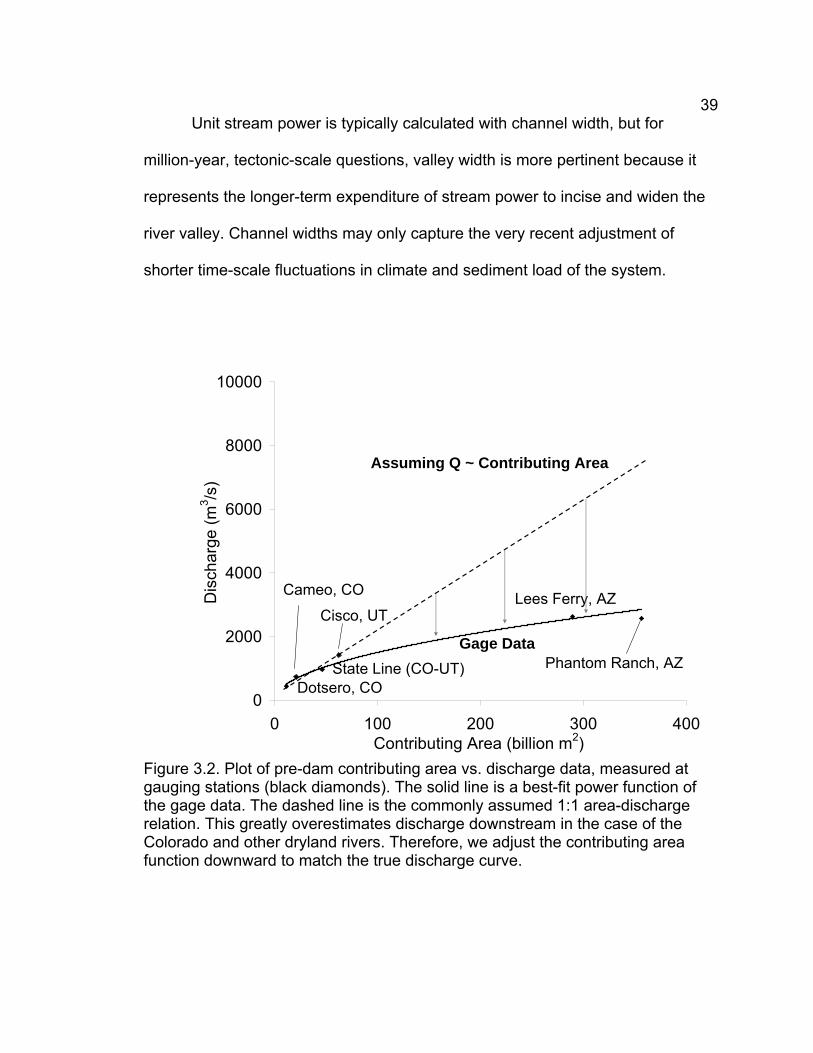
Unit stream power is typically calculated with channel width, but for
million-year, tectonic-scale questions, valley width is more pertinent because it
represents the longer-term expenditure of stream power to incise and widen the
river valley. Channel widths may only capture the very recent adjustment of
shorter time-scale fluctuations in climate and sediment load of the system.
0
2000
4000
6000
8000
10000
0 100 200 300 400Contributing Area (billion m2)
Dis
char
ge (m
3 /s)
Gage Data
Dotsero, COPhantom Ranch, AZ
Cameo, CO Lees Ferry, AZCisco, UT
State Line (CO-UT)
Assuming Q ~ Contributing Area
Figure 3.2. Plot of pre-dam contributing area vs. discharge data, measured at gauging stations (black diamonds). The solid line is a best-fit power function of the gage data. The dashed line is the commonly assumed 1:1 area-discharge relation. This greatly overestimates discharge downstream in the case of the Colorado and other dryland rivers. Therefore, we adjust the contributing area function downward to match the true discharge curve.

40
Within a geographic information system (GIS), USGS 7.5 min
topographic maps were used to digitize the portion of the drainage path. The line
was then split into 0.5 km nodes, and water surface elevations were extracted
from 10 meter DEMs at the nodes and then used to calculate local slopes. Local
slope is defined as the elevation change between points 0.25 km upstream and
downstream of each node, divided by the horizontal distance between the two
points (0.5 km). Where topography has been obscured by reservoirs and dams,
contour lines were digitized from digital USGS 7.5 min topographic maps that
include pre-dam topography. The vector contour lines were then converted to
raster format and merged with the initial 10 meter DEMs, replacing the post dam
topography with a model of the pre-dam topography.
Channel and Valley Widths
Channel widths were measured from digital 1:24,000-scale USGS
topographical maps within a GIS. Following the methods of Mackley (2005),
channel widths were measured between the water edges at 0.5 km intervals
along the profile.
We define valley width as the distance from bedrock wall to bedrock wall,
just above the level of the flood plain. Measurements were made perpendicular to
channel flow, or in areas of high sinuosity measurements were made
perpendicular to the trend of the valley. To capture the valley width the river has
acted over, at millennial or longer timescales, (since the beginning of the
Holocene), valley width was measured at 5 m above the modern channel. This

41
height was chosen based on several previous studies of alluvial stratigraphy
(e.g., Hereford et al., 1996; Grams and Schmidt, 1999; Pederson et al., 2006). It
is a typical height above the river, below which Holocene floodplain and terrace
deposits represent river activity across the valley bottom, and above which
Pleistocene deposits or bedrock are encountered. The both width measures
correlate moderately well in bedrock reaches (Fig. 3.3). The modern channel in
alluvial reaches increasingly underestimates the overall width that energy is
expended over at long timescales. Henceforth we employ only valley width due
to the time-scales of interest here.
y = 1.6869x + 55.666R2 = 0.5048
0
200
400
600
800
1000
0 40 80 120 160 200Channel Width
Val
ley
Wid
th
alluvial reaches
bedrock reaches
Figure 3.3. Plot of channel width vs. valley width, the trend line and equation are of the bedrock reaches only.

42
ksn
Our determination of ksn utilizes built-in ArcGIS tools as well as an ArcGIS
add-on and MATLAB scripts developed by Snyder et al., (2000) and Kirby et al.,
(2003). With these tools, channel elevations and upstream drainage areas were
extracted from a 75 m DEM. This 75 m DEM was resampled from 30 m DEMs,
which was necessary due to computational limitations but is certainly sufficient
for representing longitudinal profiles at our large scale of interest (cf. Cook et al.,
2009). A minimum-cell-value algorithm was utilized in resampling, wherein the
lowest cell value within a 3 x 3 moving window is assigned to the new, coarser
raster. This method was chosen to eliminate cell values that are too high in
narrow canyons and sinuous reaches due to floodplains and canyon walls during
down-sampling. Dams and reservoirs were also removed from the 75 m DEM
using the methods described above for the 10 m DEMs used in unit stream
power calculations.
Standard hydrologic tools in ArcGIS were used to fill local sinks in the
DEM, and then create flow direction and flow accumulation grids, thereby
defining drainages. MATLAB was then used to sample elevations along the flow
paths from the DEM in order to remove artificial spikes along the channel
profiles. These are generated where cell values that are too high in narrow
canyons and sinuous reaches due to floodplains and canyon walls during down-
sampling. The profile is smoothed in MATLAB using a moving average-window
of 20 km, and channel elevations are calculated over 6 m vertical intervals along

43
the profile, simulating the 20 ft contour most DEM data are derived from. The
slope of the regression line of these gradients plotted against contributing area
yields concavity (Ө). A reference concavity is needed to calculate the normalized
steepness index (ksn), and it is estimated as the average concavity of the reaches
of interest (e.g., Snyder et al., 2000; Kirby et al., 2003). A reference Ө of 0.25
was used here, as a value generally representative of the five geomorphic
reaches here (described in the next section).
To address the problem described above with assuming that contributing
area is proportional to discharge, we adjusted the flow-accumulation grid used in
the contributing area calculation using our pre-dam, effective-discharge rating
curve for the Colorado River recorded at gauging stations (Fig. 3.2). Annual
precipitation data for the climatological period 1961-90 was obtained from the
Prism Climate Group and used to capture the spatial distribution of rainfall
throughout the Colorado River basin (http://www.prism.oregonstate.edu/). We
converted the precipitation data from polygon to 75 m grid format and linearly
transformed the values by weighting the areas of highest precipitation as 1 and
areas of lowest precipitation as 0.2. The lower bound was determined through an
iterative process by adjusting the weighting value until the contributing area at
gage locations matched the discharge curve of the gages (Fig. 3.3).
Concavity
Long profile concavity at the reach scale is strongly subjective, based
upon how one chooses reaches. Ideally, reaches are defined by observed breaks

44
in the slope of the gradient-area scaling (e.g., Kirby et al., 2003). In fact, it has
the potential to be quite subjective and misleading when reaches are not chosen
by some independent criteria, especially in the case of highly irregular profiles
like that of the Colorado River. For our determinations of concavity, we define
five reaches based upon geologic province. The Green River Basin reach is
defined by Cenozoic basin fill. Older and stronger Proterozoic and Paleozoic
sedimentary rocks outcrop in the eastern Uinta Mountains reach. The Uinta
Basin reach consists of Cenozoic basin fill and older and stronger Proterozoic
and Paleozoic sedimentary rocks. The Central Plateau reach comprises mostly
Mesozoic sedimentary rocks, and the Grand Canyon reach is dominated by
Precambrian basement and Paleozoic rocks. We have therefore determined the
concavity of the river through similar rock types, rather than subjectively choosing
similar reach concavities or gradients or focusing only on knickpoints at the
breaks between reaches.
RESULTS
Unit Stream Power
Unit stream power values inevitably follow the patterns of gradient and
channel width data (Table 3.1 and Appendix B). The averaged unit stream power
of the 48 study reaches reveals great variations in energy expenditure along the
profile of the trunk stream (Fig. 3.4), with reaches of high-gradient and low width
resulting in relatively high units stream power at the four knickzones previously
outlined (Fig 3.4). Because discharge increases only slightly downstream in the

45
Colorado River (Fig. 3.2), one might expect unit stream power values to
generally decrease as width increases and slope decreases along a “normal”
stream profile, but in fact overall values in this study do not follow a pattern of
decreasing magnitude downstream. Rather, unit stream power values are
highest in the Grand Canyon reach at the most downstream knickzone, and
decrease in magnitude at each subsequent upstream knickzone.
Of the 48 reaches that values were averaged over, the reaches of highest
unit stream power are in Grand Canyon, with magnitudes as high at 630 watts/m2
in the upper Granite Gorges of Grand Canyon. Also, Grand Canyon has a great
deal of reach-scale variability, with values as low as 142 watts/m2 in the reach
just downstream of Lee’s Ferry. With an overall average across the 13 reaches of
376 watts/m2, the Grand Canyon geologic province has the largest magnitude of
unit stream power by nearly a factor of ten. In contrast, the Glen Canyon reaches
of the Central Plateau province just upstream of the Grand Canyon, has an
average value of 46 watts/m2. This is consistent with the findings Mackley (2005),
where unit stream power is nearly an order of magnitude lower in Glen Canyon
than Grand Canyon, despite their adjacency.
One of the steepest reaches, Cataract Canyon within the Central Plateau,
has a very high unit stream power of up to 441 watts/m2, with the rest of the
reaches of the Central Plateau are much lower, down to 5 watts/m2 through
bedrock in labyrinth Canyon. The Uinta Basin reaches have modest unit stream
power values ranging from 5 watts/m2 to 124 watts/m2 in Desolation and Gray

46
Canyons. Unit stream power increases upstream of the Uinta Basin as the
Green River encounters older and relatively harder rocks in Split Mountain,
Dinosaur, Lodore, and Red Canyon reaches within the eastern Uinta Mountain
Geologic province. Here, unit stream power values range from 305 watts/m2
down to 30 watts/m2 in Browns Park. The gently sloping reaches of the Green
River Basin have an average unit stream power of only 9 watts/m2 (Table 3.1).
ksn
ksn values follow similar trends as unit stream power, but only after
adjusting the flow accumulation grid for the river measured area-discharge curve,
(Fig. 3.4). The adjusted ksn does differ from unit stream power at the downstream
knickzones, where the highest values of ksn are actually found in the Cataract
Canyon knickzone, not Grand Canyon, as is the case with unit stream power.
Overall, the magnitude of ksn does not increase downstream towards Grand
Canyon as notably as unit stream power. Comparing the upstream unit stream
power to the downstream Grand Canyon province, reach-averaged ksn values
differ by 37%, whereas the difference in unit stream power between the two
provinces is more than 500%. Yet, these comparisons are only qualitative
because ksn values are dimensionless and are strongly dependent upon the
chosen reference concavity.
More specifically, although the highest value of ksn is 1.51 in Cataract
Canyon, the highest geologic province average of 0.88 is still found in the Grand
Canyon province. In Grand Canyon, individual reach averages range from 0.27

47
TABLE 3.1. SUMMARY OF REACH-SCALE TOPOGRAPHIC AND HYDRAULIC DATA

48
near Lee’s Ferry, to 1.21 in the basement rocks near Hakatai Canyon. The
lowest values of ksn, 0.001 are found in the Gunnison Valley near Green River,
Utah, and along the Green River flowing through Labyrinth and Stillwater reaches
of Canyonlands. This matches the trends of unit stream power. Reaches in Gray
and Desolation Canyon produce ksn values in the 0.62 to 0.85 range, whereas
the reaches meandering through the basin fill of the Uinta Basin have ksn values
between 0.10 and 0.16. The ksn values in the eastern Uinta Mountains geologic
province average 0.64, and vary from 0.4 in Browns Park to 1.06 in Split
Mountain Canyon. There is a notable difference in ksn and unit stream power in
the eastern Uintas. Relative to the spike seen in unit stream power, ksn values
are markedly lower in this knickzone relative to the basin reach above and below
it, with ksn being only two to three times greater in knickzones, whereas unit
stream power is nearly 15 times greater than neighboring basins.
Looking at the unit stream power and ksn data in map view (Fig. 3.5), the
trunk streams compare well. Unit stream power is relatively higher in general in
the southwestern plateau. Illustrating a strength of the ksn metric, the full suite of
tributaries of the overall drainage can be inspected for steepness variations,
where higher values are in the Colorado Rockies and the high plateaus of the
western Colorado Plateau. Notable are the low ksn values in mid-upper Lower
Colorado River, and the high values throughout the Kanab, Paria, Escalante, San
Juan and other tributaries flowing into Grand and Glen Canyons.

49
Figure 3.4. (A) Longitudinal profile of the Colorado and Green rivers, through the Colorado Plateau. River mile 0 is by convention at Lee’s Ferry, AZ. Study reaches (n = 48) and the five overall geologic provinces have been delineated based upon lithology. Plotted below this profile are reach and moving-window averages (0.5 km) of gradient (B), valley width (C), unit stream power (D), and ksn (E).

50
Figure 3.5. Map of the distribution of unit stream power (A), and discharge-adjusted normalized channel steepness index (B) of the Colorado-Green River through the Colorado Plateau.
Concavity
The remarkably irregular long profile of the Colorado and Green rivers
results in an extremely wide variation in concavity values (Fig. 3.6). The long
profile form through the Green River Basin has a classic concave shape, with a
typical concavity of 0.38 relative to other drainages (Whipple and Tucker, 1999).
In contrast, the Uinta Basin geologic province contains a large convexity with a
value of negative 2.5; a result of the low gradients of the basin followed by the
steep reaches within Desolation Canyon. The eastern Uinta Mountains, as well
as the Central Plateau and Grand Canyon provinces also have more moderate
convexities (negative values), illustrating how far this rivers profile is from the
ksn Unit Stream Power
(watts/m)
Θ ref = 0.25
A B

51theoretical graded profile of a river. The measured concavity of the three
reaches is essentially the same, ranging from negative 0.22 to negative 0.29.
The Central Plateau province incorporates the extreme Cataract Canyon
knickpoint; otherwise it would be concave.
DISCUSSION / CONCLUSIONS
Unit stream power is the most direct approach in determining reaches of a
drainage that are expelling more energy, and it has real, meaningful units that
help in quantifying variability. A map of ksn can be produced in areas where there
is not convenient gage and width data (Fig. 3.5), and it has comparable results to
Figure 3.6. Slope-area data of the Colorado River drainage trunk streams derived from DEMs. Black lines show the regressed fit for the five study geologic provinces, with the slope of the regression being the concavity (Ө). Note that the X-axis is an “effective” drainage area, modified to capture the decreasing rate of discharge increase downstream as described in the text. Large gaps or steps in the effective drainage area in the data scatter are due to major tributary junctions.

52unit stream power. However, in this setting the flow accumulation grid
must be adjusted to take into account the decreasing rate of discharge increase
though the plateau. If not adjusted, the lower reaches have ksn values twice as
high, relatively speaking, as they should be. Concavities must be calculated at
the reach scale in order to determine a reference concavity that can be used to
determine ksn. Since we chose to define our reaches based upon geologic
province, instead of relative to knickpoints, we incorporate some knickzones.
This provides a better measure of the reach and insight as to whether the
knickzones are either transient signals moving through the system or pinned in
place by rock type.
Great debate has been focused around the gradient of the Grand Canyon
reach of the Colorado River. It has been argued recently that this steep section is
a product of tectonic uplift (Karlstrom et al., 2009). Also, recent work by Cook et
al. (2009) suggests the pulse of knickpoint recession resulting from drainage
integration ~6 Ma has moved upstream of Lee’s Ferry and the Glen Canyon trunk
area, into tributaries. Mackley (2005), instead draws the conclusion that Grand
Canyon is steep because of the high strength of the bedrock at river level. The
Colorado River flowing though Paleozoic and Precambrian rocks of Grand
Canyon exerts significantly more stream power than it does in the Mesozoic
sedimentary rocks of Glen Canyon. This linkage between stream gradient and
rock type is further supported by trends upstream where river gradient is less in
less resistant and highly fractured rocks. The Green River flowing though the
53eastern Uinta Mountains geologic province exerts nearly ten times as much
stream power thorough reaches of the more resistant Uinta Mountain group as it
does through the reaches of the weaker Browns Park Formation.
The Cataract Canyon knickpoint is defined by Paleozoic and landslide
dominated reaches. Using the valley width in our determination of unit stream
power, we average over the smaller scale effects of landslides and debris fans of
smaller regions of mass movements, but Cataract Canyon is a large scale, salt-
tectonics-driven feature. For example, in Desolation Canyon the channel is
greatly narrowed due to debris fans, so the modern channel width is much
narrower than the valley width. Thus, the valley width provides a more accurate
measure of how the river has acted over at longer time scales.
To further examine this observed relation of the long profile metrics to
bedrock variations, the next chapter explores the strength of rock units at river
level and correlation of this metric with gradient, valley width, and unit stream
power.
REFERENCES
Bagnold, R.A., 1960, Sediment discharge and stream power; a preliminary announcement: U.S. Geological Survey Circular 421. 23 p.
Bull, W. B., 1990, Stream-terrace genesis Implications for soil development:
Geomorphology, v. 3, 351-367 Cook, K.L., Whipple, K.X., Heimsath, A.M., and Hanks, T.C., 2009, Rapid
incision of the Colorado River in Grand Canyon; insights from channel profiles, local incision rates, and modeling of lithologic controls: Earth Surface Processes and Landforms, v. 34, 994–1010.

54Gardner, T.W., 1983, Experimental study of knickpoint and longitudinal profile
evolution in cohesive, homogenous material: Geological Society of America Bulletin, v. 94, p. 664-672.
Hack, J.T., 1957, Studies of longitudinal stream profiles in Virginia and Maryland:
U.S. Geological Survey Professional Paper 294-B, p. 42-97. Hack, J.T., 1973, Stream profile analysis and stream-gradient index: U.S.
Geological Survey Journal of Research. v. 1, p. 421–429. Howard, A.D., 1998, Long profile development of bedrock channels: Interaction
of weathering, mass wasting, bed erosion, and sediment transport, in Tinkler, K., and Wohl, E.E., eds., Rivers over rock: Fluvial processes in bedrock channels: American Geophysical Union Geophysical Monograph 107, p. 297–319.
Howard, A.D., and Kerby, G., 1983, Channel changes in badlands: Geological
Society of America Bulletin, v. 94, p. 739-752. Howard, A.D., Seidl, M.A., and Dietrich, W.E., 1994, Modeling fluvial erosion on
regional to continental scales: Journal of Geophysical Research, v. 99, p. 13971–13986.
Karlstrom, K.E., Coblentz, D.D., Ouimet, W.B.; Kirby, E., van Wijk, J.W.,
Schmandt, B., Crossey, L.J., Crow, R., Kelley, S., McKeon, R. E., Aslan, A., Darling, A.L., Dueker, K.G., Aster, R.C., Lazear, G.D., and Hilton, D.R., 2009, Dynamic uplift of the Colorado Rockies and western Colorado Plateau in the last 6 Ma driven by mantle flow and buoyancy: Evidence from the Colorado River region: American Geophysical Union, Fall Meeting 2009, abstract #T51F-04.
Keller, E., 1986, Investigation of active tectonics: use of surfacial earth
processes. In: Wallace RE (Eds). Active tectonics studies in Geophysics: Washington, D.C., National Academy Press, p. 136–147.
Kirby, E., Whipple, K.X., Tang, W., and Chen, Z., (2003), Distribution of active
rock uplift along the eastern margin of the Tibetan Plateau: Inferences from bedrock channel longitudinal profiles, Journal of Geophysical Research., 108(B4), 2217.
Leopold, L.B., and Langbein, W.B., 1962, The concept of entropy in landscape
evolution: U.S. Geological Survey Professional Paper 500-A, 20 p.

55Leopold, L. B., and Maddock, T., Jr., 1953, The hydraulic geometry of stream
channels and some physiographic implications: U.S. Geological Survey Professional Paper 252, 56 p.
Mackin, J.H., 1948, Concept of the graded river. Bulletin of the Geological
Society of America 59, 463-512. Mackley, R.D., 2005, Relating bedrock strength to hydraulic driving forces along
the large-scale profile of the Colorado River in Glen and Grand Canyon [MS Thesis]: Logan, Utah State University, 173 p.
Merritts, D., and Vincent, K.R., 1989, Geomorphic response of coastal streams to
low, intermediate, and high rates of uplift, Mendocino triple junction region, northern California, Geological Society of America Bulletin, v. 101, p. 1373-88.
Miller, J.R., 1991, The influence of bedrock geology on knickpoint development
and channel-bed degradations along downcutting steams in south-central Indian: Journal of Geology, v. 99, p. 591-605.
Montgomery, D.R., Abbe, T.B., Buffington, J.M., Peterson, N.P., Schmidt, K.M.,
and Stock, J.D., 1996, Distribution of bedrock and alluvial channels in forested mountain drainage basins: Nature, v. 381, p. 587-589.
Pederson, J.L., Mackley, R.D., and Eddleman, J.L., (2002), "Colorado Plateau
uplift and erosion evaluated using GIS", GSA Today, v. 12, no. 8, p. 4-10. Powell, J.W., 1876, Exploration of the Colorado River of the West: Smithsonian
Institution, Washington, DC, p. 291. Schumm, S.A., and Khan, H.R., 1972, Experimental study of channel patterns,
Geological Society of America Bulletin, 83, 1755–1770. Seidl, M.A., and Dietrich, W.E., 1992, The problem of channel erosion into
bedrock: Catena, supplement, v. 23, p. 101–124. Snyder, N. P., Whipple, K.X., Tucker, G.E., and Merritts, D.J., 2000, Landscape
response to tectonic forcing: Digital elevation model analysis of stream profiles in the Mendocino triple junction region, northern California, Geological Society of America Bulletin, 112, 1250–1263.

56Stock, J.D., and Montgomery, D.R., 1999, Geologic constraints on bedrock
river incision using the stream power law: Journal of Geophysical Research, v. 104, p. 4983–4993.
Whipple, K.X., and Tucker, G.E., 1999, Dynamics of the stream-power river
incision model: Implications for the height limits of mountain ranges, landscape response time scales, and research needs: Journal of Geophysical Research, v. 104, no. B8, p. 17661–17674.
Wobus, C.W., Whipple, K.X., Kirby, E., Snyder, N.P., Johnson, J., Spyropolou,
K., Crosby, B., and Sheehan, D., 2006, Tectonics from topography: procedures, promise and pitfalls, in Willett, S., Hovius, N., Brandon, M., and Fisher, D., eds., GSA Special Penrose publication on tectonics, climate and landscape evolution: New York, Geological Society of America, p. 55-74.

57CHAPTER 4
COLORADO PLATEAU ROCK STRENGTH AND RIVER KNICKZONES—
SPATIAL DATASETS RELATING ERODABILITY TO TOPOGRAPHIC METRICS
ABSTRACT
The remarkably irregular long profile of the Colorado River has inspired
several questions about the role of knickpoint recession, tectonics, and bedrock
resistance to erosion in the landscape evolution of Grand Canyon and the
Colorado River region. Bedrock resistance to erosion has a fundamental role in
controlling topography and surface processes, yet measurements and datasets
quantifying rock strength and rock erodability are rare.
A correlation between steepness or stream power and high rock strength
would suggest that the reach-scale gradient of the Colorado River is adjusted to
maintain a balance between driving forces and resisting forces--that it is a graded
river. We have tested this hypotheses by measuring and mapping the
erodability of major bedrock units across the plateau through several
approaches, including Selby rock-mass strength (RMS) and traditional Schmidt-
hammer compressive strength at 152 sites, as well as sample tensile strength
(Brazilian splitting test) at 26 sites. These are then related to the reach-scale
slope, gradient and valley width metrics of Chapter 3.
Generally, measurements of compressive strength relate well to that of
tensile strength as well as Selby RMS scores, with major exceptions being in the

58upper reaches of the drainage, where intact-rock strength values are uniformly
higher than the same bedrock units farther south on the plateau, which may be
an artifact of sampling methods, Using Spearman rank correlation these strength
data were analyzed with respect to topographic measures from Chapter 3.
Measurements of compressive strength range from 86 to 160 MPa, occurring in
the Nankoweap and Hakatai reaches of Grand Canyon, respectively. Tensile
strength ranges from 1.4 MPa in the Entrada sandstone found in the Central
Plateau, to 11.2 MPa in the basement rocks of Grand Canyon. RMS values
follow similar trends as compressive strength, which are at a minimum of 61 in
the Shale/Carbonate reaches of the Muav and Bright Angel, and are at a
maximum in the Toroweap, Kaibab, Supai formations near Lee’s Ferry and in the
Colton in Desolation Canyon.
Results indicate that rock strength and topographic metrics are strongly
correlated in the middle-lower reaches of the plateau drainage, and that channel
steepness and width are strongly linked to rock type. This confirms the
hypothesis that where sediment supply and hillslope process are not controlling
channel morphology, bedrock acts as a direct control on the river’s width and
gradient.
INTRODUCTION
Bedrock resistance to erosion has a fundamental role in controlling
topography and surface processes, because it is a primary resisting factor. This
has been recognized since the birth of geomorphology, including by J.W. Powell

59in his trips through Grand Canyon, yet measurements and datasets quantifying
rock strength are rare. During episodes of bedrock incision, the properties of
river-level bedrock control the form, processes, and rates of river incision, and
this has been confirmed by laboratory and field observations confirm this (e.g.,
Wohl and Merritt, 2001; Sklar and Dietrich, 2001).
Strength properties of river-level bedrock exert a direct control on the
large-scale profile of a drainage by setting up its first-order template during times
when it is a bedrock river. The Colorado Plateau landscape, because of its
semiarid climate and active exhumation, is strongly influenced by variations in
bedrock. It is a prime setting to collect such a dataset of rock strength because
all bedrock units are exposed for study. The Colorado-Green trunk drainage
across the plateau has a broadly convex longitudinal profile, with four prominent,
large-scale knickzones evident: 1) The canyons of the eastern Uinta Mountains:
2) Desolation Canyon; 3) Cataract Canyon; and 4) Grand Canyon (Fig. 1 and
Chapter 3). Debate revolves around the degree to which this variable profile
represents tectonically driven, transient knickpoints, versus adjustments of
gradient directly or indirectly (via bedload) to changing bedrock properties (cf.,
Pederson et al., 2002; Hanks and Webb, 2006; Cook et al., 2009).
We hypothesize that much of the irregular profile of the river may be an
expression of dynamic equilibrium or adjustment to bedrock resistance.
In order to explore the role bedrock strength plays on the Colorado River
long profile, we have quantified the strength of the bedrock at river level across

60the plateau through three approaches: 1) compressive strength; 2) tensile
strength; and 3) Modified Selby rock-mass strength (RMS). RMS and the
Schmidt-hammer compressive strength measures included within it were
conducted at 152 sites. Site investigations were completed in this study at 11
sites within the upper reaches of Glen Canyon and Canyonlands National Park
(Fig. 4.1). The remaining site data were compiled from previous work by Larsen
(2005) in the Green River canyons of Dinosaur National Monument, Roberson
(2001) who worked within Desolation and Gray canyons, Mackley (2005) who
worked at 84 sites within Grand and Glen canyons, and work at 32 sites
previously unpublished by J. Pederson. For the laboratory determination of
tensile strength, rock samples were collected at 26 sites. Samples were collected
at 11 sites above Lake Powell by the author, and at 15 sites in Glen and Grand
Canyons by Mitchell (2005).
The goals of this study are to: a) quantify bedrock strength along distinct
bedrock reaches of the Colorado-Green trunk drainage; and b) relate those data
to reach-scale river form. Our purpose is to explore whether knickzones in the
system represent an adjustment of gradient pinned to a given bedrock setting, or
whether they may be transient features spatially independent of bedrock
patterns.

61
Figure 4.1. Map of the upper Colorado River catchment above Lake Mead, showing the drainage path analyzed, and the location of the complied RMS study sites (red dots) and 11 study sites investigated by the author (yellow dots).

62BACKGROUND
Bedrock Incision Processes
The hydrologic events needed to accomplish bedrock incision are of low-
frequency and high magnitude (Tinkler, 1971), which adds to the difficulty in
understanding the process (Miller, 1991). During periods of bedrock conditions,
the variables that control incision include discharge of the river, sediment supply
and grain size, tectonic uplift or base level fall, and the resistance of the bedrock
to erosion (Hack, 1957). Based upon these controlling factors, a river adjusts its
grade and width to develop an equilibrium profile.
Because their effect is poorly constrained, rock strength, sediment supply,
grain size, and other factors influencing bedrock erosion have been lumped into
a rock erodability coefficient (k), for use in numerical landscape evolution
models. In an effort to better understand the role of sediment supply, grain size
and rock strength in landscape evolution, Sklar and Dietrich (2001) use
laboratory experiments to investigate relations between sediment supply and
erosion rate, as well as rock strength and erosion rate. Using an “abrasion mill”
and Brazilian tension splitting tests (Vutukuri et al., 1974), they are able to
determine a log-linear regression relating tensile strength to erosion rate.
Importantly, they confirm Gilbert’s (1877) assertion that sediment supply is
directly linked to bedrock-incision rate. They confirm that too much sediment can
begin to armor the streambed, effectively decreasing the incision rate into

63bedrock, and too little sediment does not provide the necessary “tools” to
erode the bedrock.
Graded Profile of Bedrock Streams
A graded longitudinal profile, specifically for alluvial rivers, is commonly
associated with a smooth, concave profile, free of knickzones (Mackin, 1948).
However, not all rivers with irregular long profiles are ungraded or out of
equilibrium, especially in the case of bedrock streams. Physical modeling of
knickpoint behavior by Gardner (1983) illustrated that the upstream migration of
knickpoints through the fluvial system over time is dependent on the
characteristics of the bedrock, spatially varied climate, and increasing sediment
load can produce knickzones in the longitudinal profile. For example, a reach of
river where the stream bed is insolated by an over abundance of sediment, would
not incise at the same rate as a reach where the sediment is mobilized during
flood flows, exposing the stream bed for incision (Schumm and Khan, 1972;
Keller, 1986; Howard, 1998). Varying bedrock type along a streams length can
create knickzones when a base level fall signal incises quickly through weak rock
and becomes hung up on more resistant rocks. Miller (1991) found channel
morphology to be related to the structural properties of underlying bedrock, and
convexities and knickzones in the long profile may be adjustments to bedrock
variations.

64Colorado River as a Mixed Bedrock-Alluvial River
The Colorado River drainage, as we experience it today is a mixed
bedrock/alluvial river system (Howard et al., 1994). The whitewater canyons are,
to most observers, obviously bedrock river reaches. However, reaches in which
bedrock is exposed along the channel bottom and/or edges alternate with
reaches that are alluviated. This is not uncommon (e.g. Miller, 1991; Seidl and
Dietrich, 1992; Wohl, 1992, 1993). In addition to this spatial variability, there has
been variability in the periods of time when particular reaches, even if alluvial in
the present day, would be considered bedrock rivers, incising into bedrock and
creating features such as Grand Canyon. We suggest that the large-scale
template for the Colorado and Green river’s gradient and long profile may be set
during or inherited from these bedrock-stream episodes, even in reaches that are
alluvial today.
Creation of the Colorado River Profile after Base Level Fall
The Colorado River flowing across the Colorado Plateau encounters a
range of rock types, and it is believed to be a relatively young feature. The
Colorado River was only integrated into its current drainage basin by ~6 Ma, and
a 1000+ m base level fall off the west edge of the Colorado Plateau was
ultimately caused by this integration (e.g., Pederson et al., 2002). A rapid base
level fall of this magnitude would inevitably produce a transient knickpoint that
would migrate far upstream. It is likely that the steep reaches of the Colorado
River are ultimately inherited from this signal.

65An analysis of incision rates and tributary gradients in close proximity to
Glen Canyon by Cook et al. (2009), has lead them to believe a pulse of incision
has moved through Grand and Glen Canyons within the past ~ 500 ky, and
tributaries to the Colorado are continuing to adjust to this pulse of incision of the
main stem. Cook et al. (2009) suggest that the large contrast in gradient between
Grand Canyon and Glen Canyon is neither the upstream extent of Grand Canyon
incision nor solely related to lithology, but instead results from a combination of
lithologic and transient effects. Numerical model results presented by Pelletier
(2010) support the timing and magnitude of a ~6 Ma base-level fall, which is
responsible for the rapid incision of the Colorado River through Grand and
Marble canyons. This baselevel fall at 6 to 2 Ma, was then followed by cliff
retreat, isostatic rebound, and fault-controlled incision.
In studying knickpoint initiation and distribution in fluvial networks, Crosby
and Whipple (2006) found very few knickpoints in weak substrates. Yet in harder,
more coherent units, most tributaries with relatively smaller drainage areas
contained knickpoints. We surmise that knickpoints of the Colorado Plateau in
softer units either degraded in a diffusive manner as seen in Gardner’s
experiments (1983), or never formed in the first place.
Howard et al. (1994) hypothesize that the irregular profile of the Colorado
River in Grand Canyon is controlled by coarse sediment brought into the main
channel from tributaries. Thus, the caliber and volume of bed material becomes a
direct control and bedrock becomes an indirect control on incision rates. They

66propose that the gradient of the river through Grand Canyon is controlled by
the production and mobilization of coarse debris from local tributaries, and that
the thinning of alluvium would likely accelerate bedrock erosion.
METHODS
Mechanical reaches
Following the same approach as chapter 3, forty-eight reaches along the
Colorado-Green trunk drainage of distinct bedrock type were defined for this
study. This allows statistical comparison of rock strength to hydraulic parameters
for the same reaches. Rock units at river level have been grouped at the reach
scale, wherein units are mechanically similar. For example, the basement schist,
gneiss, granite and pegmatites found in Grand Canyon reaches have been
grouped together. Where rock units in particular reaches were not sampled due
to logistical and time constraints, data from the same bedrock units in other
reaches were substituted.
Study sites
Rock-strength data collected in this study and compiled from others
include intact-rock strength measured with a Schmidt Hammer, fracture spacing,
and other characteristics associated with Selby rock-mass strength (RMS) at
over 152 sites along the drainage (Fig. 1). Field investigations were completed at
fresh, unweathered, rock outcrops at river level.

67 For tensile strength analysis, rock samples were collected at a total of
26 sites in this and previous studies conducted at Utah State University.
Whenever possible, samples were collected from fresh outcrops at river level.
Where this was not possible, samples were selected from fresh talus, carefully
examined to ensure there was no weathering rind or fractures.
Friable rocks, such as shales and weakly cemented sandstones, could not
be measured for rock strength or tensile strength. For example, the shales of the
Mancos and Chinle formations have intact-rock strengths and tensile strengths
below the minimum tolerances, or were too friable to test with the methods used
in this study. This affects six reaches, and these shale reaches are excluded
from subsequent analysis.
Methods of Measurement
A common approach to quantifying rock erodability is the Selby rock-mass
strength (RMS) scale, a method developed for analyzing hillslope stability (e.g.,
Selby, 1980; Allison et al., 1993). The RMS scale used here was enhanced by
Moon (1984) by subdividing the rating scales for intact rock strength and the
spacing of partings. This enhanced scale is sometimes referred to as a modified
Selby RMS classification. The semi-quantitative index is used to capture the
effects of jointing and other features at outcrops, and utilizes in situ compressive
strength as measured with a Schmidt hammer. Specifically, the RMS score is
summed from seven variables that are rated in value, including: 1) intact-rock
strength (Schmidt hammer rebound percent); 2) weathering; 3) fracture spacing;

684) fracture orientation; 5) fracture continuity; 6) fracture width; and 7)
groundwater.
At each of the investigation sites, repeat Schmidt hammer measurements
(n ≥ 50) were obtained from fresh rock surfaces, free of fractures in the area of
the measurement to the degree possible. Some rock types are repeated at up to
three reaches along the river profile, thus some rock types have up to 150
Schmidt Hammer measurements. These rebound values are averaged and the
mean rebound value is then converted to compressive strength (C) using the
equation:
06.1*12.2 RC = (1)
where R is the mean rebound value and 2.12 and 1.06 are coefficients obtained
by Selby (1980) through empirical testing.
Fracture characterization at each site was based upon criteria outlined by
Selby (1993), relating to how fractures favor either stability or erosion of
hillslopes. For example, few and widely spaced fractures receive a lower score
than fractures that occur in high frequency and are closely spaced. Bedrock that
has widely-spaced fractures exhibits increased resistance to plucking and
abrasion, as blocks are either immovably large or wear down more slowly.
For the determination of tensile strength, rocks samples were collected in
the field and brought back to the lab where they were cored and cut into disks. A
drill press equipped with water feed equipment was set up with a 2-inch inner-
diameter, diamond-coated drill bit to core the rock samples. These cylinders

69where then cut into 1-inch think disks using a standard rock saw. At least ten
disks of each rock type were then subjected to the Brazilian splitting test method
the standard procedure for tensile strength (Vutukuri, et al., 1974; Selby, 1980),
at the Utah State University Structural Engineering lab. The test is conducted by
applying a uniaxial stress to the disk, set on edge, until a primary fracture forms
parallel to the loading vector across the disk. Because there is no confining
pressure, the disks are able to split or fail in tension. Tensile strength was
calculated using the following equation (ASTM, 2001):
LDpσt π
2= (2)
where σt (MPa) is tensile strength in megapascals, p (N) is the load at failure in
newtons, L (mm) is the thickness of each disk in millimeters, and D (mm) is the
diameter of each disk in millimeters.
Statistical Analysis
Correlations between unit stream power, valley width, and gradient from
Chapter 3, as well as Selby RMS, field-compressive strength and laboratory
tensile strength from this and other compiled studies were evaluated using the
non-parametric Pearson correlation coefficient.
RESULTS
Rock strength results are shown in Table 4.1 and found in Appendix C,
with reach-averaged unit stream power imported from Chapter 3. Results show

70reach-averaged measures of compressive strength that range from 86 to 160
MPa, tensile strength that ranges from 1 to 12 MPa, and Selby RMS scores that
range from 61 to 79.
The highest compressive strength for bedrock, at 160 MPa, is found within
Grand Canyon in the Proterozoic basement granite, schist, gneiss and
pegmatites. Other rock units that are nearly as strong (i.e., greater than 150
MPa) include the Morgan and Madison units in the Uinta Mountains, the Honaker
Trail limestone in Cataract Canyon, the Kaibab limestone at Lee’s Ferry.
Likewise, the highest tensile strength values, 11 to 12 MPa, are found in the
same rock units, as well as Quaternary basalt flows located in western Grand
Canyon.
The lowest values of compressive strength (86 MPa) are also in Grand
Canyon, with the silt and sandstone of the Bright Angel shale. Other low values
ranging from 92 to 103 MPa, are from the Jurassic sandstones of the central
plateau. The lowest reach averaged values of tensile strength at 1-2 MPa are
found in the same Jurassic sandstones and mudstones in Labyrinth canyon north
of the confluence of the Green and Colorado rivers. The shale reaches
throughout the study area are presumably the weakest of all, though not
measurable by these means.

71TABLE 4.1. SUMMARY OF REACH-SCALE ROCK-STRENGTH AND HYDRAULIC DATA1

72Table 4.1. CONTINUED
Overall trends in the rock strength of individual units (as opposed to reach
averages) indicate that older rocks, such as the Proterozoic granite, gneiss,
schist, quartzite, pegmatite, and Proterozoic sandstones within Grand Canyon
are the strongest rock units tested, (Fig. 4.2). Somewhat younger Paleozoic
sandstones and limestones average 130 MPa in compressive strength and 6
MPa in average tensile strength. These rocks are stronger than the younger
Mesozoic and Cenozoic basin fill sandstones of the Green River and Uinta
basins averaging approximately 118 MPa in compressive strength and 3 MPa in
tensile strength. These younger rocks have not experienced the same burial
depth as the Paleozoic rocks, thus they are less compacted and cemented. The
igneous basalt in western Grand Canyon is relatively young but is inherently
stronger than the sedimentary rocks due to its crystalline texture.

73
Figure 4.2. Comparison of rock type and age to mean tensile and field-compressive strength.
A plot of compressive strength to tensile strength reveals a scatter in the
data that is poorly fit with a trend line (Fig. 4.3). There does however appear to
be some correlation between these two metrics, and with more sampling a better
correlation coefficient maybe determined.
In terms of our third measure of rock strength, Selby RMS has the highest
values of 78-79 in the Proterozoic basement reaches and the upper Paleozoic
rocks of the Lee’s Ferry reach within Grand Canyon, as well as in the Colton and
Weber sandstone reaches of the northern plateau. The lowest RMS value, 56 is
in the upper Jurassic sandstone and mudstone of the Carmel, Entrada, and
Curtis sandstone reaches

74
R2 = 0.21
0.0
2.0
4.0
6.0
8.0
10.0
12.0
14.0
50 100 150
compressive strength (MPa)
tens
ile s
treng
th (M
pa)
0
Figure 4.3. Relation between reach-scale averages of compressive and tensile strength.
Rocks with higher strength correspond spatially to knickzones and
reaches of high unit stream power. The Cataract knickzone has a mean tensile
strength of 10 MPa and unit stream power value averages 262 watts/m2. Peak
local-average unit stream power values of 441 watts/m2 are found within reaches
of Grand Canyon, where consistently high values of unit stream power averaging
376 watts/m2, peaking at 594 watts/m2. The values also correlate to high average
values of tensile strength at 8 MPa, and peak at 12 MPa. Conversely, reaches of
relatively low unit stream power consistently coincide with values of low rock
strength. For example, the sandstones and mudstones in the Gunnison Valley
averages ~37 watts/m2 in unit stream power and 2.7 MPa in tensile strength.
Statistical analysis confirms a weak correlation between reach averages of
compressive strength and unit stream power (Fig. 4.4), as well as between Selby

75RMS and unit stream power (Fig. 4.5). The correlation between tensile
strength and unit stream power (Fig. 4.6) is the strongest correlation (Table 4.2).
R2 = 0.14
0100200300400500600700800900
1000
50 100 150
compressive strength (MPa)
unit
stre
am p
ower
(wat
ts/m
2 )
0
Figure 4.4. Relation between reach-scale averages of compressive strength and unit stream power.
R2 = 0.26
0
100
200
300
400
500
600
700
50 60 70 80
Selby RMS
unit
stre
am p
ower
(wat
ts/m
2 )
0
Figure 4.5. Relation between reach-scale averages of Selby RMS and unit stream power.

76
R2 = 0.45
0
0.0005
0.001
0.0015
0.002
0.0025
0.003
0.0035
0.0 5.0 10.0 15.0
tensile strength (MPa)
stre
am g
radi
ent (
m/m
)
Figure 4.6. Relation between reach-scale averages of tensile strength and stream gradient.
TABLE 4.2. CORRELATIONS BETWEEN BEDROCK-RESISTING AND HYDRAULIC-DRIVING FORCES
Compressive strength
Tensile strength
Selby RMS
Tensile strength 0.50 Selby RMS 0.46 0.42
Unit stream power 0.53 0.75 0.53 Gradient 0.59 0.81 0.49
Valley Width -0.21 -0.72 -0.38 Note: Results from Spearman rank correlation (Rs) of reach-average values of hydraulic-driving forces to bedrock-resisting forces, within reaches that have been studied.
DISCUSSION / CONCLUSIONS
With the inclusion of compressive or intact-rock strength (Schmidt hammer
test) in the Selby RMS score, it is not surprising that Selby RMS scores and
measures of compressive strength follow similar trends across the plateau. With
the exception of outliers, the general trend in tensile strength follows trends in
compressive strength. In the Uinta Basin and the eastern Uinta Mountain
geologic provinces, compressive strength values are uniformly higher by 10 to 20

77MPa than predicted by the strength of those same rock units in more southerly
reaches. This disparity may be an artifact of Schmidt hammer sampling methods
by other researchers, or it could be that the rocks are unpredictably stronger.
Results indicate moderate correlations exist between rock tensile strength,
gradient, and unit stream power. In particular, rocks high in tensile strength
correspond to steeper reaches and higher energy expenditure. Weaker
correlations between gradient and compressive strength and with Selby RMS
exist. Since rivers erode in more of a plucking and abrasion process, that is
captured better with measures of tensile strength, it is not surprising that gradient
is better correlated to tensile strength, than compressive strength or RMS.
It is of note that there are no knickzones found in reaches of relatively weak rock,
and any steepness anomalies are associated with harder rocks. This could be
the result of transient knickpoints propagating through weak rock units very
quickly such that none remain in those reaches today. Alternatively, it could
indicate that the long profile of the Colorado River up to Glen Canyon has
adjusted to baselevel fall and is in a dynamic equilibrium with rock strength.
These findings are similar to that of Cook et al. (2009), where they suggest that a
baselevel fall signal has propagated up through at least Glen Canyon in the trunk
streams, and is presently found in the tributaries as seen by convex reaches at
nearly the same elevations.

78
Figure 4.7. (A) Longitudinal profile of the Green and Colorado rivers flowing across the Colorado Plateau, including 48 study reaches presented in Table 1. Below this are reach averages of Selby RMS (B), tensile strength (C), and compressive strength (D), and unit stream power (E). Geologic provinces are outlined with vertical dashed lines. Tics on long profile indicate reach breaks and arrows point to the location of major tributaries confluences. nd= no data.

79These results generally support the idea that the Colorado drainage is
dynamically adjusted to meet the demands of varying rock types during erosion.
This implies that reach-scale knickzones are mostly not transient features,
although they are inevitably the result of baselevel fall. Tensile strength seems to
be the best measure, but more tensile data are needed in the upper regions of
the Colorado River Drainage, before an analysis like this is complete.
REFERENCES
Allison, R.J., Goudie, A.S., and Cox, N.J., 1993, Geotechnical properties of rock masses: Their control on slope form and mechanisms of change along the Napier Range, western Australia: Geomorphology, v. 8, p. 65-80.
Cook, K.L., Whipple, K.X., Heimsath, A.M., and Hanks, T.C., 2009, Rapid
incision of the Colorado River in Grand Canyon; insights from channel profiles, local incision rates, and modeling of lithologic controls. Earth Surface Processes and Landforms, v. 34, 994–1010.
Crosby, B.T., Whipple, K.X., 2006, Knickpoint initiation and distribution within
fluvial networks: 236 waterfalls in the Waipaoa River, North Island, New Zealand: Geomorphology, v. 82, no. 1-2.
Gardner, T.W., 1983, Experimental study of knickpoint and longitudinal profile
evolution in cohesive, homogenous material: Geological Society of America Bulletin, v. 94, p. 664-672.
Gilbert, G.K., 1877, Report on the Geology of the Henry Mountains: Washington,
D.C., Government Printing Office. Hack, J.T., 1957, Studies of longitudinal stream profiles in Virginia and Maryland:
United States Geological Survey Professional Paper, 294B, 94 p. Hanks, T.C., and Webb, R.H., 2006, Effects of tributary debris on the longitudinal
profile of the Colorado River in Grand Canyon: Journal of Geophysical Research, v. 111, 13 p.
Howard, A.D., 1998, Long profile development of bedrock channels: Interaction
of weathering, mass wasting, bed erosion, and sediment transport, in

80Tinkler, K., and Wohl, E.E., eds., Rivers over rock: Fluvial processes in bedrock channels: American Geophysical Union Geophysical Monograph v. 107, p. 297–319
Howard, A.D, Dietrich, W.E., and Seidl, M.A., 1994, Modeling of fluvial erosion on
regional to continental scales: Journal of Geophysical Research, v. 99, no. B7, p. 13,971-13,986.
Keller, E., 1986, Investigation of active tectonics: use of surfacial earth
processes. In: Wallace, R.E. (ed.), Active tectonics studies in Geophysics: Washington, D.C., National Academy Press, p. 136–147
Larsen, I.J., 2003, From the Rim to the River: The geomorphology of debris flows
in the Green River Canyon of Dinosaur National Monument, Colorado and Utah [MS Thesis]: Logan, Utah State University, 86 p.
Mitchell, K.J., 2005, Bedrock tensile strength and the Colorado River through
Glen and Grand Canyons [Senior Thesis]: Logan, Utah State University, 21 p.
Mackley, R.D., 2005, Relating bedrock strength to hydraulic driving forces along
the large-scale profile of the Colorado River in Glen and Grand Canyon. [MS Thesis]: Logan, Utah State University, 165 p.
Miller, J.R., 1991, The influence of bedrock geology on knickpoint development
and channel-bed degradations along downcutting steams in south-central Indian: Journal of Geology, v. 99, p. 591-605.
Moon, B.P., 1984, Refinement of a technique for determining rock mass strength
for geomorphological purposes: Earth Surface Processes and Landforms, v. 9, p. 189-193.
Pederson, J.L., Mackley, R.D., and Eddleman, J.L.., 2002, "Colorado Plateau
uplift and erosion evaluated using GIS", GSA Today, v. 12, no. 8, p. 4-10. Pelletier, J.D., 2010, Numerical modeling of the late Cenozoic geomorphic
evolution of Grand Canyon, Arizona, Geological Society of America Bulletin, v. 122 p.
Roberson, P., 2001, Rock-strength control in Desolation and Gray Canyons of
the Green River, A river landscape in dynamic equilibrium [MS Thesis]: Logan, Utah State University, 86 p.

81Schumm, S.A., and Khan, H.R., 1972, Experimental study of channel patterns,
Geological Society of America Bulletin, 83, p. 1755–1770. Seidl, M.A., and Dietrich, W.E., 1992, The problem of channel erosion into
bedrock: Catena, supplement, v. 23, p. 101–124. Selby, M.J., 1980, A rock mass strength classification for geomorphic purposes:
With tests from Antarctica and New Zealand: Zeitschrift fur Geomorphologie, v. 24, p. 31-51.
Selby, M.J., 1993, Hillslope materials and processes: Oxford, U.K., Oxford
University Press, 451 p. Sklar, L.S., and Dietrich, W.E., 2001, Sediment and rock strength controls on
river incision into bedrock: Geology, v. 29, no. 12, p. 1087-1090. Tinkler, K.J., 1971, Active valley meanders in south-central Texas and their wider
implications. Geological Society of America Bulletin, v. 82, no. 7, p. 1783-1800.
Vutukuri, V. S., Lama, R. D., and Saluja, S.S., 1974, Handbook on mechanical
properties of rocks. Volume 1: Testing techniques and results: Bay Village, Ohio, Trans Tech Publishers, 280 p.
Wohl, E.E., 1992, Bedrock benches and boulder bars: Floods in the Burdekin
Gorge of Australia, Geological Society of America Bulletin, v. 104, p. 770 -778.
Wohl, E.E., 1993, Bedrock channel incision along Picanniny Creek, Australia.,
Geological Society of America Bulletin, v. 101, p. 749 -761. Wohl, E.E., and Merritt, D.M., 2001, Bedrock channel morphology: Geological
Society of America Bulletin, v. 113, no. 9, p. 1205-1212.
82CHAPTER 5
SUMMARY
This Thesis includes three chapters, each a separate study, linked by the
common theme of erosion in the Colorado Plateau. Here, the conclusions of
each chapter are summarized.
Terrestrial Lidar monitoring of creep at a cultural site in Grand Canyon
We found that ground-based lidar surveys can indeed track surface-
particle creep in the setting of Grand Canyon. A significant fraction of the clasts
tracked at the site moved above the change-detection threshold of 3 cm over the
timeframe between any two scans. This study, with a relatively small data set of
only two surveys, does not show the expected positive relations of creep rate to
slope or clast size, although it does not preclude the existence of such relations
either.
More frequent scans at supplementary sites are needed to identify and
develop functional relations to characterize the creep processes degrading
archaeological sites within the river corridor of Grand Canyon. High contrast
scans and new image-drape technology should be utilized for monitoring of this
sort in the future.
Large-scale Metrics of the Colorado River Drainage
In our comparison of methods of identifying knickzones and analyzing the
longitudinal profile of the Colorado River drainage, we acknowledge that unit

83stream power is the most direct approach in determining energy expenditure of
streams at the reach scale, having mechanically meaningful units that help in
quantifying variability. Where stream gage data is unavailable or time is limited
for the calculation of unit stream power, a weighted flow accumulation grid can
be used to develop a map of ksn, which is comparable to unit stream power. In
order to do this, though, the flow accumulation grid must be adjusted to take into
account the decreasing rate of discharge increase downstream through the
plateau.
Concavity must be calculated for each reach in order to determine an
overall reference concavity that can be used to determine ksn. We chose to
define our reaches based upon geologic province, instead of relative to
knickpoints, and this provides a better measure of the reach and insight as to
whether the knickzones are transient signals moving through the system or are
pinned in place by rock type.
We use valley width instead of channel width in our determination of unit
stream power in order to integrate influences such as Holocene debris fans over
the smaller time and spatial-scale. For example, in Desolation Canyon where the
channel is confined by large debris fans, the modern channel width is much
narrower than the overall valley width. The valley width provides a more
appropriate measure of the river’s erosive action over longer, late Cenozoic time
scales.

84The Colorado River flowing though the Paleozoic and Precambrian rocks of
Grand Canyon exerts significantly more stream power than it does in the
Mesozoic sedimentary rocks of Glen Canyon. This linkage between stream
gradient or energy expenditure and rock type is further supported by trends
upstream, where river gradient is less in weaker and highly fractured rocks. For
example, the Green River flowing though the eastern Uinta Mountains geologic
province exerts nearly ten times as much stream power thorough reaches of the
more resistant Uinta Mountain group as it does through the reaches of the
weaker Browns Park Formation.
Colorado Plateau Rock Strength and River Knickzones
This study, comparing the metrics of river steepness and energy
expenditure to a dataset of measured rock strength, involved more than one set
of measurements. We quantified rock strength in 3 ways: 1) in situ compressive
strength; 2) laboratory tensile strength; and 3) Modified Selby rock-mass strength
(RMS), at sites across the plateau.
Results indicate that Selby RMS scores and measures of compressive
strength follow similar trends across the plateau, which is not surprising
considering that compressive strength (Schmidt hammer test) is included in the
Selby RMS score. More significantly, the general trend in tensile strength follows
trends in compressive strength. Tensile strength seems to be the best measure,
but more tensile data are needed in the upper regions of the Colorado River
Drainage before an analysis like this is complete.

85Results indicate that moderate correlations exist between rock tensile
strength, gradient, and unit stream power. In particular, rocks high in tensile
strength correspond to steeper reaches and higher energy expenditure.
Correlations between gradient and compressive strength and with Selby RMS
exist, but are weaker. Since rivers erode bedrock by plucking and abrasion
processes, which are captured better with measures of tensile strength, it is not
surprising that gradient is best correlated to tensile strength.
In the Uinta Basin and the eastern Uinta Mountain geologic provinces,
compressive strength values are uniformly higher by 10 to 20 MPa than predicted
by the strength of those same rock units in more southerly reaches. This disparity
may be an artifact of varying Schmidt hammer methods employed in the datasets
compiled here, or it could be that the rocks are unpredictably stronger.
It is of note that there are no knickzones found in reaches of relatively
weak rock; all steepness anomalies are associated with harder rocks. This could
be the result of transient knickpoints propagating through weak rock units very
quickly, such that the transient signal remains “hung up” in only steep reaches
today. Alternatively, it could indicate that the long profile of the Colorado River
has adjusted to baselevel fall and is in a dynamic equilibrium with rock strength
as it erodes through this landscape. These results generally support the idea that
the Colorado drainage is dynamically adjusted to meet the demands of varying
rock types during erosion. This implies that reach-scale knickzones are mostly
not transient features, although they are inevitably the result of baselevel fall.

86
APPENDICES

87APPENDIX A.
REGISTERED LIDAR SCANS SUPPORTING CHAPTER 2
Folder: 60 mile scan data May 2006 Files: Brian Collins field notes May 2006 Lidar Control – 60 Mile May 2006 Scan file - mile60-05062006_Ultra_1reg Scan file - mile60-05062006_Ultra_2reg Scan file - mile60-05062006_Ultra_3reg Scan file - mile60-05062006_Ultra_4reg Scan file - mile60-05062006_Ultra_5reg Scan file - mile60-05062006_Ultra_6reg Folder: Photographs May 2006 Files: Location of Lidar Reflector 1 and 2 May 2006 Location of Lidar Reflector 3 May 2006 Location of Scanner May 2006 Folder: 60 mile scan data May 2007 Files: Lidar Control – 60 Mile May 2007 Scan file - Scan file - mile60-052005_Ultra_7reg
Folder: Photographs May 2007 Files: Location of Lidar Reflector 1 May 2007 Location of Lidar Reflector 2 May 2007 Folder: 60 mile scan data September 2007 Files: Lidar Control – 60 Mile September 2007 Scan file - mile60-052007_Ultra_7_reg
Folder: Photographs September 2007 Files: Location of Lidar Reflector 1 Sept 2007 Location of Lidar Reflector 2 Sept 2007 Location of Lidar Reflector 3 Sept 2007 Study hillslope Sept 2007

88
APPENDIX B.
TOPOGRAPHIC DATA OF THE COLORADO RIVER DRAINAGE (CD)

89APPENDIX C.
SUMMARY OF STATISTICS ON ROCK STRENGTH.
Table C.1 In situ strength - Joel Pederson Table C.2 In situ strength – Rob Mackley Table C.3 In situ strength – Paul Roberson Table C.4 In situ strength – Isaac Larsen Table C.5 In situ strength – This study Table C.6 Tensile strength – Kelly Mitchell Table C.7 Tensile strength – This study

Tabl
e C
.1. R
OC
K S
TRE
NG
TH D
ATA
Dat
a so
urce
: J
oel P
eder
son
unpu
blis
hed
Riv
er M
ile(L
ee's
Fer
ry =
0)
Roc
k un
itLi
thol
ogy
n= A
vgSD
Min
Q1
Med
ian
Q3
Max
Inta
ct-r
ock
stre
ngth
(S
chm
idt H
amm
er)
Spac
ing
Orie
ntat
ion
cont
inui
tyW
idth
Wea
ther
ing
Gro
undw
ater
RM
S sc
ore
955
96
141
861
4564
0.2483
8207.5
08.1405
enitrevartL75
576
96
541
5102
6685
0.2500.54
4304.8
00.1505
wolF tlasabL802
wolF tlasabR5.802
6019
1714
56
86
750.
0S
hina
rum
p C
ong.
sand
ston
e50
42.9
06.
2028
40.0
042
.048
5718
2114
54
96
77S
outh
Kai
bab
trail
Kai
bab
limes
tone
5055
.10
5.50
4551
.25
55.0
5869
2021
145
59
680
~3.5
RLo
wer
Kai
bab
Fm/u
pper
Tor
owea
p50
53.1
07.
9038
46.2
554
.059
6820
2114
65
96
81S
outh
Kai
bab
trail
Coc
onin
osa
ndst
one
5049
.60
4.70
3847
.00
50.0
5258
1815
145
49
671
20.5
RE
spla
nade
sand
ston
e50
55.3
06.
1040
52.0
054
.060
6620
2114
56
96
81 276
96
541
5171
7594
0.3400.83
4206.8
04.2405
mF igimohata
WR5.02
886
95
541
8212
1736
0.7552.25
9303.7
00.7505
mF igimohata
WR5.02 34
.7L
Red
wal
llim
esto
ne50
60.8
04.
4047
.00
62.0
6468
2121
146
49
580
56R
Mua
vlim
esto
ne50
41.6
010
.60
2034
.25
42.0
4962
188
144
45
558
56R
Brig
ht A
ngel
Fm
shal
e/lim
esto
ne50
34.8
05.
0026
32.0
034
.038
5012
1514
16
55
58 845
57
141
88
8463
0.1305.62
0207.6
05.1305
elahsmF legn
A thgirB
L75 209L
Brig
ht A
ngel
Fm
sand
ston
e52
178
145
59
664
65.6
LTa
peat
ssa
ndst
one
5042
.10
8.40
3136
.00
40.0
4664
1421
144
69
674
61.5
LTa
peat
ssa
ndst
one
5050
.50
7.30
3046
.00
50.0
5666
1815
145
49
671
206.
6RTa
peat
ssa
ndst
one
6720
1914
56
96
79 476
96
641
5181
0684
0.5400.24
2300.6
08.5405
sanedraC
L6.5627
69
55
4151
8136
355.54
00.8392
00.906.54
05sanedra
CR76
975
96
441
1202
3726
0.2600.45
4402.7
03.8505
mF xoD
L4.5666
69
64
418
9176
160.64
52.5342
05.3102.74
05mF xo
DR76 75
.3L
Shi
num
oQ
uartz
ite64
2028
146
59
688
78R
Bas
s Fm
6319
2514
45
76
80etinarg
L90265
2015
144
59
673
etinargR87
6620
1514
56
66
72etinarg
R2.80258
188
185
69
670
tsihcsL902
5718
1314
45
96
69tsihcs
R2.80254
1821
186
59
683
ssiengL7.712
7022
1514
55
96
76ssieng
L5.32248
1415
144
56
462
serutcarFseulaV dnuober re
mma
H tdimhcS
Tabl
e C
.1. R
OC
K S
TRE
NG
TH D
ATA
91

Tabl
e C
.2. R
ock
Stre
ngth
Dat
aD
ata
sour
ce:
Mac
kley
, R.D
., 20
05, R
elat
ing
bedr
ock
stre
ngth
to h
ydra
ulic
driv
ing
forc
es a
long
the
larg
e-sc
ale
prof
ile o
f the
Col
orad
o R
iver
in G
len
and
Gra
nd C
anyo
n. T
hesi
s, U
tah
Sta
te U
nive
rsity
.
Site
XY
ZR
ock
unit
Lith
olog
yn=
Avg
SDM
in Q
1M
edia
nQ
3M
axIn
tact
-roc
k st
reng
th
(Sch
mid
t Ham
mer
)Sp
acin
gO
rient
atio
nco
ntin
uity
Wid
thW
eath
erin
gG
roun
dwat
erR
MS
scor
e1
4488
6340
8034
114
14N
avaj
o
sand
ston
e50
32.9
05.
9025
2831
.037
475
2814
55
76
702
4486
9640
8033
713
68N
avaj
o
sand
ston
e50
45.4
04.
6036
4245
.048
5614
2114
55
76
723
4485
9140
8040
513
04K
ayen
ta
sand
ston
e20
33.2
05.
7024
3032
.035
505
2114
55
96
654
4484
6740
8025
111
22W
inga
te
sand
ston
e30
52.2
02.
6048
4953
.554
5614
2114
55
96
745
4485
1540
8009
711
04W
inga
te
sand
ston
e30
54.1
02.
9049
5155
.057
5814
2114
55
96
746
4475
5140
8000
196
0C
hinl
e
cong
lom
erat
e43
35.2
05.
2022
3135
.039
4810
2114
54
76
677
4595
3740
8283
513
41P
age
sa
ndst
one
5033
.00
2.40
2831
33.0
3539
521
145
57
562
856
1177
4179
950
1634
Chi
nle
lim
esto
ne50
48.3
05.
6038
4448
.052
6014
2114
54
56
699
5604
0941
8003
515
60C
hinl
e
shal
e
1941
.20
5.10
3238
40.0
4551
1415
145
45
663
1056
0409
4180
035
1562
Chi
nle
sh
ale
31
41.9
06.
5032
3541
.049
5314
2114
54
56
6911
5594
9441
7986
514
26M
oenk
opi
silts
tone
5046
.20
5.10
3542
47.5
4958
1428
145
47
678
1255
9494
4179
865
1426
Moe
nkop
i sh
ale
50
36.7
05.
8020
3436
.541
4810
1514
55
56
6013
5338
6141
4678
612
40P
age
sa
ndst
one
5038
.10
4.60
2835
38.0
4247
1028
145
55
572
1455
2898
4194
466
1158
Org
an R
ock
silts
tone
5048
.70
3.60
4246
49.0
5156
1421
145
59
573
1555
2091
4193
541
1173
Org
an R
ock
silts
tone
5048
.90
3.80
4245
49.0
5255
1428
145
55
576
1650
5309
4123
391
1348
Nav
ajo
sa
ndst
one
5039
.20
2.60
3537
40.0
4145
1021
145
59
670
1750
5309
4123
391
1348
Nav
ajo
sa
ndst
one
5035
.90
2.20
3134
36.0
3841
1021
145
59
670
1845
7227
4089
163
1152
Nav
ajo
sa
ndst
one
5036
.50
3.40
3234
35.0
3944
530
145
57
672
1942
3163
4039
834
908
Red
wal
l lim
esto
ne50
58.5
03.
3050
5658
.561
6518
2114
55
76
7620
4232
5540
4014
093
9R
edw
all
limes
tone
5056
.10
3.30
4955
56.5
5862
1821
145
57
474
2142
3217
4040
198
981
Red
wal
l lim
esto
ne28
58.1
03.
7050
5658
.562
6418
2114
55
75
7522
4229
5540
4004
110
00W
atah
omig
isa
ndst
one
5052
.20
5.10
4248
53.0
5560
1821
145
57
676
2342
3029
4040
315
1143
Wes
coga
me
sand
ston
e50
57.9
02.
7051
5658
.060
6218
1514
55
96
7224
4191
1340
3766
6W
esco
gam
e sa
ndst
one
5058
.10
4.40
5054
58.0
6265
1821
145
59
678
2541
7117
4036
460
1465
Coc
onin
o
sand
ston
e50
57.1
03.
7047
5558
.059
6418
2114
55
76
7626
4170
0140
3658
2K
aiba
b
limes
tone
2657
.30
2.80
5255
57.5
6062
1830
145
57
685
2744
6002
4078
696
1606
Kai
bab
lim
esto
ne50
59.5
03.
7052
5659
.562
6820
2114
55
75
7728
4243
4140
4158
988
0R
edw
all
limes
tone
3248
.40
3.90
4346
47.0
5160
1421
145
57
571
2942
3007
4040
304
Man
akac
ha
sand
ston
e50
54.9
04.
7048
5054
.558
6418
2114
55
96
7830
4231
4140
4030
210
62M
anak
acha
si
ltsto
ne50
38.5
010
.20
2230
38.5
4660
1421
145
57
672
3142
4733
4036
288
1062
Red
wal
l lim
esto
ne50
52.7
05.
0042
5052
.057
6318
2814
55
76
8332
4224
4640
1817
910
62B
right
Ang
shal
e
5028
.00
7.60
1122
29.0
3445
515
145
55
554
3342
1923
4018
346
914
Brig
ht A
ngsh
ale
50
30.2
06.
4019
2530
.036
425
2114
55
56
6134
4215
6440
1827
898
1M
uav
lim
esto
ne80
37.1
08.
7020
3235
.542
6010
2114
55
75
6735
4213
7440
1838
410
00M
uav
lim
esto
ne50
38.2
05.
6026
3439
.043
4810
2114
55
76
6836
4217
7940
1834
692
7M
uav
lim
esto
ne30
40.0
06.
4030
3538
.046
5214
2114
55
75
7137
4252
9840
1299
387
8B
right
Ang
shal
e
3016
.40
4.40
1012
15.5
2024
515
145
55
554
3842
8209
4005
446
Tape
ats
sa
ndst
one
5050
.90
4.50
4048
50.5
5460
1815
145
59
672
3942
7011
3999
903
869
Dox
sa
ndst
one
5063
.50
4.30
5061
63.5
6772
2015
145
59
674
4041
0980
3989
990
Vis
hnu
sc
hist
30
63.4
03.
8057
6064
.066
7020
2114
55
96
8041
4109
8039
8999
0Zo
roas
ter
gran
ite
3059
.30
5.60
5056
58.5
6270
1821
145
59
678
4240
8112
3991
911
762
Vis
hnu
sc
hist
50
61.2
06.
1042
5760
.567
7120
2114
55
96
8043
4001
5039
9524
274
9V
ishn
u
schi
st
3054
.60
4.80
4850
54.5
5864
1821
145
59
577
4440
0150
3995
242
749
Zoro
aste
r gr
anite
30
51.3
04.
6045
4950
.053
6518
2114
55
95
7745
3975
1939
9568
581
4Zo
roas
ter
gran
ite
3056
.00
4.00
5052
55.5
5963
1821
145
59
678
4639
4839
3995
528
735
Zoro
aste
r gn
eiss
50
63.5
05.
9050
6164
.068
7320
2114
55
76
7847
3922
6739
9515
973
1V
ishn
u
schi
st
3060
.70
5.80
4559
61.5
6569
2021
145
57
678
4839
0909
3995
528
731
Vis
hnu
gn
eiss
50
60.8
04.
6051
5860
.064
7020
2114
55
96
8049
3898
7339
9645
373
1V
ishn
u
schi
st
3051
.50
4.50
4448
51.0
5364
1815
145
59
672
5039
0221
3995
927
719
Vis
hnu
sc
hist
30
56.5
04.
3047
5456
.060
6418
2114
55
96
7851
3897
4739
9643
071
3V
ishn
u
gnei
ss
5056
.60
5.40
4852
56.0
6170
1821
145
59
678
5238
9723
3996
461
713
Zoro
aste
r gr
anite
50
60.8
04.
6050
5860
.064
6920
2114
55
96
8053
3892
4339
9728
869
5V
ishn
u
schi
st
3059
.00
3.90
5156
59.0
6265
1821
145
59
678
5438
5674
4000
414
692
Zoro
aste
r gr
anite
30
58.3
04.
8045
5658
.062
7018
1514
55
96
7255
3793
7740
1102
669
5B
ass
lim
esto
ne50
59.7
04.
3049
5660
.563
6820
2114
55
76
7856
3696
6240
0664
764
6Zo
roas
ter
gran
ite
3062
.00
4.20
5359
63.0
6469
2021
145
59
680
5736
7667
4011
682
655
Tape
ats
sa
ndst
one
5039
.40
4.60
3036
39.5
4448
1415
145
57
565
5836
7667
4011
682
655
Tape
ats
sa
ndst
one
5056
.10
4.40
4552
56.5
5964
1821
145
57
575
Schm
idt H
amm
er re
boun
d Va
lues
Frac
ture
s Z
one
12 N
AD
27
Tabl
e C
.2. R
OC
K S
TRE
NG
TH D
ATA
100

5931
5693
4008
993
536
Brig
ht A
ngsa
ndst
one
6041
.70
8.20
2835
41.5
4858
1415
145
55
462
6031
3135
4007
942
543
Brig
ht A
ngsa
ndst
one
5050
.50
4.70
4247
50.5
5460
1815
145
55
567
6130
0789
3998
094
491
basa
lt
basa
lt50
57.6
04.
3048
5458
.061
6618
2114
55
96
7862
3000
8439
9688
848
2ba
salt
ba
salt
3056
.00
3.60
5053
56.5
5963
1821
145
59
678
6329
3664
3996
948
488
Mua
v
limes
tone
5035
.90
3.70
3033
35.0
3850
1021
145
57
668
6444
2515
4068
715
1079
Toro
wea
p
sand
ston
e61
55.9
05.
3048
5055
.061
6518
2114
55
96
7865
4422
7940
6923
710
09C
ocon
ino
sa
ndst
one
5054
.90
3.70
4852
54.0
5763
1821
145
59
678
6644
2181
4069
327
991
Her
mit
si
ltsto
ne30
39.0
05.
2030
3638
.042
5210
2114
55
56
6667
4421
8140
6932
799
1H
erm
it
shal
e30
12.2
02.
609
1011
.513
205
1514
55
56
5568
4419
1540
6955
197
5H
erm
it
silts
tone
3056
.20
2.60
5055
56.0
5861
1421
145
55
670
6944
1915
4069
551
975
Her
mit
sh
ale
3013
.10
2.70
1011
12.0
1520
515
145
55
655
7044
1628
4069
758
963
Her
mit
sh
ale
30
25.7
07.
3015
2025
.030
425
1514
55
56
5571
4425
3940
6881
310
36To
row
eap
sa
ndst
one
5055
.40
3.90
4553
55.5
5962
1821
145
57
676
7228
5966
3957
301
576
Tape
ats
sa
ndst
one
5060
.40
3.00
5458
60.0
6268
1821
145
59
678
7328
2283
3952
327
866
Mua
v
limes
tone
6048
.90
5.30
4045
49.0
5360
1415
145
55
664
7427
8645
3947
138
1033
Mua
v
limes
tone
5056
.80
3.90
4454
57.0
6064
1821
145
57
676
7542
5142
4028
642
1402
Coc
onin
o
sand
ston
e30
49.8
02.
7045
4849
.052
5514
2114
55
76
7276
4251
1040
2859
613
72E
spla
nade
sa
ndst
one
6055
.10
2.90
4954
55.0
5762
1821
145
57
676
7754
2502
4206
239
1332
Kay
enta
sa
ndst
one
5039
.50
3.10
3438
39.5
4148
1021
145
55
666
7854
4794
4201
631
1317
Win
gate
sa
ndst
one
5043
.90
2.60
3942
44.0
4649
1428
145
59
681
7942
6818
3999
218
832
Car
dena
s
basa
lt
5049
.70
5.20
4146
48.5
5461
1415
145
55
563
8042
2199
3993
441
834
Dox
silts
tone
5054
.90
4.00
4652
55.0
5863
1821
145
59
678
8142
0439
3990
354
1013
Dox
sa
ndst
one
5052
.70
3.60
4250
52.5
5561
1821
145
57
575
8241
8580
3989
257
795
Shi
num
o
quar
tzite
3060
.40
3.90
5158
61.0
6368
1815
145
59
672
8341
9075
3989
742
811
Shi
num
o
quar
tzite
5058
.50
2.70
5456
58.0
6065
1821
145
59
678
8441
6593
3989
173
802
Hak
atai
sa
ndst
one
6046
.20
8.00
3042
46.5
5260
1421
145
57
672
Tabl
e C
.2. C
ON
TIN
UE
D
101

Tabl
e C
.3. R
ock
Stre
ngth
Dat
aD
ata
sour
ce:
Rob
erso
n, P
., 20
01, R
ock-
stre
ngth
con
trol i
n D
esol
atio
n an
d G
ray
Can
yons
of t
he G
reen
Riv
er, A
rive
r lan
dsca
pe in
dyn
amic
equ
ilibr
ium
. The
sis,
Uta
h S
tate
Uni
vers
ity.
Riv
er M
ile(L
ee's
Fer
ry =
0)
Roc
k un
itLi
thol
ogy
n=A
vgSD
Min
Q1
Med
ian
Q3
Max
Inta
ct-r
ock
stre
ngth
(S
chm
idt H
amm
er)
Spac
ing
Orie
ntat
ion
cont
inui
tyW
idth
Wea
ther
ing
Gro
undw
ater
RM
S sc
ore
-434
.8G
reen
Riv
ersa
ndst
one
5052
.00
52.0
6218
814
65
76
64-4
23.9
Gre
en R
iver
sand
ston
e50
57.0
058
.066
1815
94
49
667
-405
.3C
olto
nsa
ndst
one
100
45.0
046
.054
1421
185
69
679
-404
.6C
olto
nsa
ndst
one
100
51.0
051
.066
1821
185
67
677
-396
.6C
olto
nsa
ndst
one
100
54.0
054
.065
1821
186
57
681
-380
.4N
orth
Hor
nlim
esto
ne50
50.0
035
.547
1015
96
67
654
-379
.8N
orth
Hor
nlim
esto
ne51
50.0
051
.060
1815
96
46
661
-376
.0N
orth
Hor
nlim
esto
ne50
50.0
050
.054
1421
185
46
677
-375
.4Fl
agst
aff
limes
tone
5057
.00
57.0
6618
1514
66
66
76-3
75.4
Flag
staf
flim
esto
ne50
47.0
047
.562
1415
146
66
664
-361
.5G
ray
Can
yon
sand
ston
e77
-360
.7G
ray
Can
yon
sand
ston
e79
-359
.9G
ray
Can
yon
sand
ston
e73
Schm
idt H
amm
er re
boun
d Va
lues
Frac
ture
s
Tabl
e C
.3. R
OC
K S
TRE
NG
TH D
ATA
102
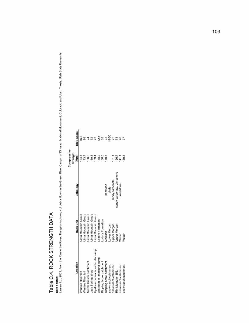
Tabl
e C
.4. R
ock
Stre
ngth
Dat
aD
ata
sour
ce:
Lars
en, I
.J.,
2003
, Fro
m th
e R
im to
the
Riv
er: T
he g
eom
orph
olog
y of
deb
ris fl
ows
in th
e G
reen
Riv
er C
anyo
n of
Din
osau
r Nat
iona
l Mon
umen
t, C
olor
ado
and
Uta
h. T
hesi
s, U
tah
Sta
te U
nive
rsity
.
Loca
tion
Roc
k un
itLi
thol
ogy
Com
pres
sive
Stre
ngth
(Mpa
)R
MS
scor
eW
inni
es R
iver
left
Uin
ta M
ount
ain
Gro
up16
4.1
76.5
Win
nies
Riv
er le
ftU
inta
Mou
ntai
n G
roup
173.
786
Mid
dle
Dia
ster
cat
chm
ent
Uin
ta M
ount
ain
Gro
up16
6.5
74Ja
ck S
prin
gs d
raw
Uin
ta M
ount
ain
Gro
up16
9.8
72U
pstre
am o
f wad
e an
d cu
rtis
cam
pU
inta
Mou
ntai
n G
roup
159.
473
upst
ream
of l
imes
tone
cam
pLo
dore
For
mat
ion
138.
272
.5R
ippl
ing
broo
k ca
tchm
ent
Lodo
re F
orm
atio
n13
0.5
68R
ippl
ing
broo
k ca
tchm
ent
Mad
ison
limes
tone
170.
778
snow
ranc
h ca
tchm
ent
Low
er M
orga
nsh
ale
45-5
0sn
ow ra
nch
catc
hmen
tU
pper
Mor
gan
sand
y ca
rbon
ate
161.
172
RM
kilo
met
er 3
53.1
Upp
er M
orga
nsa
ndy
carb
onat
e, L
imes
tone
156.
771
snow
ranc
h ca
tchm
ent
Web
ersa
ndst
one
141.
176
snow
ranc
h ca
tchm
ent
Web
er13
9.4
77
Tabl
e C
.4. R
OC
K S
TRE
NG
TH D
ATA
103

Tabl
e C
.5. R
ock
Stre
ngth
Dat
aD
ata
sour
ce:
This
stu
dy
XY
Roc
k un
itLi
thol
ogy
n= A
vgSD
Min
Q1
Med
ian
Q3
Max
Inta
ct-r
ock
stre
ngth
(S
chm
idt H
amm
er)
Spac
ing
Orie
ntat
ion
cont
inui
tyW
idth
Wea
ther
ing
Gro
undw
ater
RM
S sc
ore
6258
1342
7338
9W
inga
tesa
ndst
one
5056
.00
3.00
5054
56.0
5862
1828
165
59
687
6159
7042
8339
5S
alt W
ash
sand
ston
e50
55.0
03.
0042
5355
.056
5818
2618
52
106
8560
7059
4297
738
Bru
shy
Bas
insa
ndst
one
5054
.00
7.00
4249
55.0
5965
1828
115
47
679
5849
7544
6034
7D
uche
sne
Riv
er fm
sand
ston
e50
56.0
03.
0050
5357
.058
6218
2116
55
95
7956
9474
4257
010
Nav
ajo
sand
ston
e50
50.0
04.
0039
4850
.052
5818
2814
55
95
8457
3554
4290
489
Ent
rada
sand
ston
e50
38.0
03.
0032
3538
.040
4610
2314
55
96
7261
6882
4262
571
Ele
phan
t Can
yon
near
Plim
esto
ne50
47.0
08.
0032
4047
.053
6314
2118
55
96
7861
6882
4262
571
Hon
aker
Tra
il ne
ar P
otas
limes
tone
5055
.00
5.00
4352
56.0
6063
1815
95
49
565
6173
6942
6197
5C
edar
Mes
asa
ndst
one
5050
.00
4.00
4048
51.0
5357
1824
145
49
680
6174
6942
6200
5C
edar
Mes
asa
ndst
one
5050
.00
4.00
4045
51.0
5356
1828
116
69
684
5697
5941
9803
9H
onak
er T
rail
Abo
ve H
it elim
esto
ne50
50.0
08.
0026
4552
.055
5918
2814
55
95
84
Schm
idt H
amm
er re
boun
d Va
lues
Frac
ture
sU
TM Z
one
12 N
AD
83
Tabl
e C
.5. R
OC
K S
TRE
NG
TH D
ATA
104

Table C.6. Rock Strength DataData source:Mitchell, K.J., 2005, Bedrock Tensile Strength and the Colorado River through Glen and Grand Canyons. Senior Thesis, Utah State University.
Brazilian Splitting Test Results
Rock Unit NameRockType
SampleName
Disk#
Diameter(mm)
Thickness
(mm)Mass
(g)
Load atfailure
(lb)
Load atfailure
(N)
TensileStrength
(MPa)Basement (granite) granite PE lin g RM84.5 1 50.6 23.01 118.42 1598.39 7,110.00 3.89Basement (granite) granite PE lin g RM84.5 2 50.6 23.26 119.83 1364.59 6,070.00 3.28Basement (granite) granite PE lin g RM84.5 3 50.6 22.02 114.89 1636.61 7,280.00 4.16Basement (granite) granite PE lin g RM84.5 4 50.6 24.50 125.99 1775.99 7,900.00 4.06Basement (granite) granite PE lin g RM84.5 5 50.6 27.10 142.12 1773.74 7,890.00 3.66Granite (Diamond Creek) granite DC Granite 1 50.6 24.36 131.20 3190.04 14,190.00 7.33Granite (Diamond Creek) granite DC Granite 2 23.92 50.60 124.65 2913.52 12,960.00 6.82Pegmatite (Cottonwood Pegmatite Complex) granite 03-08 1 50.6 23.94 124.60 2893.29 12,870.00 6.76Pegmatite (Cottonwood Pegmatite Complex) granite 03-08 2 50.6 24.56 130.00 1425.29 6,340.00 3.25Kaibab limestone Kb LS 1 50.6 23.24 110.70 1454.51 6,470.00 3.50Kaibab limestone Kb LS 2 50.6 22.38 106.80 1303.89 5,800.00 3.26Kaibab limestone Kb LS 3 50.6 22.30 105.30 1616.38 7,190.00 4.06Kaibab limestone Kb LS 4 50.6 22.95 108.10 1850.18 8,230.00 4.51Kaibab limestone Kb LS 5 50.6 19.48 92.80 2371.73 10,550.00 6.81Kaibab limestone Kb LS 6 50.6 25.56 127.50 2326.77 10,350.00 5.09Kaibab limestone Kb LS 7 50.6 22.46 105.40 1569.17 6,980.00 3.91Kaibab limestone Kb LS 8 50.6 25.14 124.40 2212.12 9,840.00 4.92Kaibab limestone Kb LS 9 50.6 24.06 117.90 2009.79 8,940.00 4.67Kaibab limestone Kb LS 10 50.6 24.22 113.67 1985.06 8,830.00 4.59Kaibab limestone Kb LS 11 50.6 23.24 107.43 1180.25 5,250.00 2.84Muav limestone Muav RM 148 1 25.32 50.60 136.81 914.97 4,070.00 2.02Muav limestone Mv LS2 1 50.6 23.04 125.80 2257.08 10,040.00 5.48Muav limestone Mv LS2 2 50.6 24.11 130.10 2311.04 10,280.00 5.36Muav limestone Mv LS2 3 50.6 24.98 128.00 2293.05 10,200.00 5.14Muav limestone Mv LS2 4 50.6 26.09 140.00 2594.29 11,540.00 5.56Muav limestone Mv LS2 5 50.6 26.06 135.60 3297.95 14,670.00 7.08Muav Limestone limestone Mv LS 1 1 50.6 26.52 138.08 2074.35 9,227.17 4.38Muav Limestone limestone Mv LS 1 2 50.6 26.14 137.289 1997.98 8,887.44 4.28Muav Limestone limestone Mv LS 1 3 50.6 25.82 133.453 2852.17 12,687.10 6.18Redwall limestone Redwall 03-01A 1 50.6 25.06 131.90 1580.41 7,030.00 3.53Redwall Limestone (base of redwall) limestone Base Redwall 03-04 1 50.6 25.94 131.186 1876.96 8,349.11 4.05Redwall Limestone (base of redwall) limestone Base Redwall 03-04 2 50.6 24.68 129.395 2290.54 10,188.84 5.19Basement (metamorphics) amphibolite PE amp RM93.5 1 50.6 23.18 117.21 2407.70 10,710.00 5.81Basement (metamorphics) amphibolite PE amp RM93.5 2 50.6 22.34 114.00 2362.74 10,510.00 5.92Basement (metamorphics) schist 03-09 1 50.6 24.32 127.15 3783.53 16,830.00 8.71Basement (metamorphics) schist 03-09 2 50.6 18.34 100.69 3378.88 15,030.00 10.31Basement (metamorphics) schist 03-09 3 50.6 22.84 120.07 2108.71 9,380.00 5.17Schist Amphibolite schist PE Schist RM129L 1 25.8 50.60 152.62 5393.17 23,990.00 11.70Schist Amphibolite schist PE Schist RM129L 2 24.94 50.60 138.34 6177.75 27,480.00 13.86Schist Amphibolite schist Phantom 03-11 1 50.6 21.40 116.00 3556.48 15,820.00 9.30Schist Amphibolite schist Phantom 03-11 2 25.84 50.60 136.39 2724.68 12,120.00 5.90Dox (Escalante Creek Member) psandstone P Dox esc. c. 1 50.6 24.18 132.30 3147.32 14,000.00 7.28Dox (Escalante Creek Member) psandstone P Dox esc. c. 2 50.6 24.26 133.00 5525.80 24,580.00 12.75Dox (Escalante Creek Member) psandstone P Dox esc.c. 3 24.7 50.60 124.98 1647.85 7,330.00 3.73Dox (Escalante Creek Member) psandstone P Dox esc.c. 4 24.89 50.60 121.60 1695.06 7,540.00 3.81Dox (Escalante Creek Member) psandstone P Dox esc.c. 5 22.64 50.60 113.29 1506.22 6,700.00 3.72Dox (Escalante Creek Member) psandstone P Dox esc.c. 6 25.88 50.60 129.73 1922.12 8,550.00 4.16Dox (Solomon Temple) psandstone P Dox Sol. T. mem. 1 50.6 24.45 125.70 3158.57 14,050.00 7.23Dox (Solomon Temple) psandstone P Dox Sol. T. mem. 2 50.6 23.86 120.90 4129.74 18,370.00 9.69Dox (upper shinamu) psandstone P Dox upper shinamu 1 24.82 50.60 128.96 2677.47 11,910.00 6.04Dox (upper shinamu) psandstone P Dox upper shinamu 2 23.88 50.60 122.99 3115.85 13,860.00 7.30Dox (upper shinamu) psandstone P Dox upper shinamu 3 24.56 50.60 128.25 3111.36 13,840.00 7.09Dox (Upper Solomon Temple) psandstone Dox 03-1O 1 50.6 22.68 117.90 4833.39 21,500.00 11.93Dox (Upper Solomon Temple) psandstone Dox 03-1O 2 50.6 25.87 135.50 3466.55 15,420.00 7.50Supai Lower (Watahomigi & Manakacha) sandstone PP LS 3 50.6 23.03 114.70 1758.01 7,820.00 4.27Bright Angel sandstone BA SST RM173 1 50.6 23.58 125.40 4808.66 21,390.00 11.41Bright Angel sandstone BA SST RM173 2 50.6 26.24 131.70 5689.91 25,310.00 12.14Bright Angel sandstone BA SST RM173 3 50.6 26.42 139.70 6867.91 30,550.00 14.55Bright Angel sandstone BA SST RM173 4 50.6 24.28 128.20 3682.37 16,380.00 8.49Coconino sandstone Co SS 7 50.6 25.04 115.58 1459.01 6,490.00 3.26Coconino sandstone Co SS 8 50.6 23.62 108.25 710.40 3,160.00 1.68Coconino sandstone Co SS 9 50.6 24.90 107.79 1285.91 5,720.00 2.89Coconino sandstone Co SS 10 50.6 23.68 109.45 899.24 4,000.00 2.13Coconino sandstone Co SS 11 50.6 24.56 113.93 1144.28 5,090.00 2.61Coconino Sandstone sandstone Co SS 4 25.2 50.60 113.72 973.42 4,330.00 2.16Coconino Sandstone sandstone Co SS 5 24.62 50.60 112.08 1616.38 7,190.00 3.67Coconino Sandstone sandstone Co SS 6 24.06 50.60 108.72 1436.53 6,390.00 3.34Coconino Sandstone sandstone Co SS 1 50.6 27.62 124.497 2603.08 11,579.09 5.27Coconino Sandstone sandstone Co SS 2 50.6 26.84 122.631 2494.99 11,098.25 5.20Coconino Sandstone sandstone Co SS 3 50.6 23.96 108.366 2417.44 10,753.30 5.65Esplanade (lower) sandstone Bott Es 1 50.6 26.4 127.234 1366.23 6,077.30 2.90Esplanade (lower) sandstone Bott Es 2 50.6 25.38 126.006 2001.50 8,903.12 4.41Esplanade (lower) sandstone Bott Es 3 50.6 26.64 131.415 2123.70 9,446.68 4.46Esplanade (middle) sandstone Mid Es 1 50.6 25.16 118.537 2115.47 9,410.09 4.71Esplanade (middle) sandstone Mid Es 2 50.6 25.06 118.537 2202.42 9,796.85 4.92Esplanade (middle) sandstone Mid Es 3 50.6 26.02 122.699 2912.10 12,953.66 6.26Esplanade (middle) sandstone Mid Es 4 50.6 25.28 117.716 1705.41 7,586.05 3.78Esplanade (upper) sandstone Top Es 3 50.6 22.96 116.46 1290.40 5,740.00 3.15Esplanade (upper) sandstone Top Es 4 50.6 24.72 126.00 1393.82 6,200.00 3.16Esplanade (upper) sandstone Top Es 1 50.6 22.28 126.105 2001.50 8,903.12 5.03Esplanade (upper) sandstone Top Es 2 50.6 24.78 111.464 2371.61 10,549.47 5.36Kayenta sandstone Ky SS2 1 50.6 24.16 109.00 1279.16 5,690.00 2.96Kayenta sandstone Ky SS2 2 50.6 23.96 107.10 1058.85 4,710.00 2.47Kayenta sandstone Ky SS2 3 50.6 23.14 107.30 1310.64 5,830.00 3.17
Table C.6. ROCK STRENGTH DATA
105

Kayenta sandstone Ky SS2 4 50.6 25.11 116.30 1180.25 5,250.00 2.63Kayenta sandstone Ky SS2 5 50.6 24.11 107.00 1135.29 5,050.00 2.64Kayenta sandstone Ky SS2 6 50.6 24.44 110.70 989.16 4,400.00 2.27Kayenta sandstone Ky SS2 7 50.6 25.00 112.90 899.24 4,000.00 2.01Kayenta sandstone Ky SS2 8 50.6 24.50 111.20 1396.06 6,210.00 3.19Kayenta sandstone Ky SS2 9 50.6 24.03 108.40 1753.51 7,800.00 4.08Kayenta Sandstone sandstone Ky SS 1 50.6 27.86 119.923 3714.60 16,523.35 7.46Kayenta Sandstone sandstone Ky SS 2 50.6 27.18 119.319 3014.32 13,408.36 6.21Moenkopi mudstone Mo SS1 3 50.6 25.46 124.13 1562.42 6,950.00 3.43Moenkopi mudstone Mo SS1 4 50.6 26.36 122.21 1348.85 6,000.00 2.86Moenkopi mudstone Mo SS1 5 50.6 23.92 116.71 1029.62 4,580.00 2.41Moenkopi mudstone Mo SS2 1 50.6 25.74 131.30 2248.09 10,000.00 4.89Moenkopi mudstone Mo SS2 2 50.6 27.12 139.90 2677.47 11,910.00 5.53Moenkopi mudstone Mo SS3 1 50.6 23.82 114.00 816.06 3,630.00 1.92Moenkopi mudstone Mo SS3 2 50.6 26.08 123.00 1175.75 5,230.00 2.52Moenkopi mudstone Mo SS3 3 50.6 25.24 123.80 1333.12 5,930.00 2.96Moenkopi mudstone Mo SS3 4 50.6 26.05 132.90 1207.22 5,370.00 2.59Moenkopi Sandstone sandstone Mo SS 1 1 50.6 26.88 123.495 2091.97 9,305.56 4.36Moenkopi Sandstone sandstone Mo SS 1 2 50.6 26.4 107.847 1386.17 6,165.98 2.94Navajo sandstone Nv SS 4 50.6 25.30 114.12 699.16 3,110.00 1.55Navajo sandstone Nv SS 5 50.6 23.86 110.04 593.50 2,640.00 1.39Navajo sandstone Nv SS 6 50.6 25.34 116.01 753.11 3,350.00 1.66Navajo sandstone Nv SS 7 50.6 25.54 115.90 818.30 3,640.00 1.79Navajo sandstone Nv SS 8 50.6 24.34 112.06 656.44 2,920.00 1.51Navajo sandstone Nv SS 9 50.6 26.34 117.59 959.93 4,270.00 2.04Navajo sandstone Nv SS 10 50.6 25.40 112.99 995.90 4,430.00 2.19Navajo sandstone Nv SS 11 50.6 25.20 110.50 912.72 4,060.00 2.03Navajo sandstone Nv SS 12 50.6 26.10 116.65 1045.36 4,650.00 2.24Navajo Sandstone sandstone Nv SS 1 1 50.6 25.64 117.734 1058.98 4,710.56 2.31Navajo Sandstone sandstone Nv SS 1 2 50.6 23.48 107.772 1280.62 5,696.49 3.05Navajo Sandstone sandstone Nv SS 1 3 50.6 26.98 118.029 1020.28 4,538.41 2.12Supai (Manakacha) sandstone Lower Manakacha 03-01B 1 50.6 23.52 124.20 1355.60 6,030.00 3.23Supai (Manakacha) sandstone Lower Manakacha 03-01B 2 50.6 24.00 127.00 2517.86 11,200.00 5.87Supai (Manakacha) sandstone Lower Manakacha 03-01B 3 50.6 23.83 119.70 2113.20 9,400.00 4.96Supai (Manakacha) sandstone Manakacha 03-03 1 50.6 24.72 124.081 2712.35 12,065.15 6.14Supai Lower (Watahomigi & Manakacha) sandstone PP LS 1 50.6 23.64 124.10 2196.38 9,770.00 5.20Supai Lower (Watahomigi & Manakacha) sandstone PP LS 2 50.6 22.94 120.80 2016.54 8,970.00 4.92Supai Lower (Watahomigi & Manakacha) sandstone PP LS 4 26.36 50.60 131.30 1040.87 4,630.00 2.21Supai Lower (Watahomigi & Manakacha) sandstone PP LS 5 26.62 50.60 137.28 1166.76 5,190.00 2.45Supai Lower (Watahomigi & Manakacha) sandstone PP LS 6 23.8 50.60 115.46 892.49 3,970.00 2.10Supai Lower (Watahomigi & Manakacha) sandstone PP LS 7 25.4 50.60 126.13 1382.57 6,150.00 3.05Tapeats sandstone Tp SS 7 50.6 24.30 120.72 2643.75 11,760.00 6.09Tapeats Sandstone sandstone Tp SS 2 25.02 50.60 122.27 2711.20 12,060.00 6.06Tapeats Sandstone sandstone Tp SS 3 25.68 50.60 119.20 2423.44 10,780.00 5.28Tapeats Sandstone sandstone Tp SS 4 21.98 50.60 104.11 2556.08 11,370.00 6.51Tapeats Sandstone sandstone Tp SS 5 25.88 50.60 127.34 2598.79 11,560.00 5.62Tapeats Sandstone sandstone Tp SS 6 25.48 50.60 122.20 2272.82 10,110.00 4.99Tapeats Sandstone sandstone Tp SS 1 50.6 25.9 128.862 6257.22 27,833.48 13.52Wingate sandstone W-2 4 50.6 26.23 103.26 260.78 1,160.00 0.56Wingate sandstone W-2 5 50.6 25.16 97.29 224.81 1,000.00 0.50Wingate sandstone W-2 6 50.6 24.26 90.66 582.26 2,590.00 1.34Wingate sandstone W-2 7 50.6 26.46 102.40 656.44 2,920.00 1.39Wingate sandstone W-2 8 50.6 24.34 93.79 580.01 2,580.00 1.33Wingate sandstone W-2 9 50.6 26.28 100.16 577.76 2,570.00 1.23Wingate Sandstone sandstone W-1 1 50.6 26.64 95.155 520.69 2,316.15 1.09Wingate Sandstone sandstone W-1 2 50.6 25.56 91.227 608.65 2,707.40 1.33Wingate Sandstone sandstone W-2 1 50.6 27.58 104.837 728.27 3,239.49 1.48Wingate Sandstone sandstone W-2 2 50.6 26.58 96.123 533.59 2,373.54 1.12Wingate Sandstone sandstone W-2 3 50.6 24 92.235 613.34 2,728.26 1.43
Table C.6. CONTINUED
106

Table C.7. Rock Strength DataData source:This study
Brazilian Splitting Test Results
Rock Unit NameRockType
SampleName
Disk#
Diameter(mm)
Thickness
(mm)Mass
(g)
Load atfailure
(lb)
Load atfailure
(N)
TensileStrength
(MPa) X YSalt Wash sandstone Salt Wash-1 1 50.8 25 2350 10453 5.24 615970 4283395Salt Wash sandstone Salt Wash-2 2 50.8 23 1410 6272 3.42 615970 4283395Salt Wash sandstone Salt Wash-3 3 50.8 23 2160 9608 5.24 615970 4283395Salt Wash sandstone Salt Wash-4 4 50.8 23 2700 12010 6.54 615970 4283395Salt Wash sandstone Salt Wash-5 5 50.8 23 2760 12277 6.69 615970 4283395Salt Wash sandstone Salt Wash-6 6 50.8 23 2350 10453 5.70 615970 4283395Salt Wash sandstone Salt Wash-7 7 50.8 23 2100 9341 5.09 615970 4283395Salt Wash sandstone Salt Wash-8 8 50.8 24 3100 13789 7.20 615970 4283395Salt Wash sandstone Salt Wash-9 9 50.8 23 1740 7740 4.22 615970 4283395Salt Wash sandstone Salt Wash-10 10 50.8 23 1570 6984 3.81 615970 4283395Navajo sandstone Navajo-1 1 50.8 23 360 1601 0.87 569474 4257010Navajo sandstone Navajo-2 2 50.8 23 460 2046 1.11 569474 4257010Navajo sandstone Navajo-3 3 50.8 23 380 1690 0.92 569474 4257010Navajo sandstone Navajo-4 4 50.8 23 340 1512 0.82 569474 4257010Navajo sandstone Navajo-5 5 50.8 23 460 2046 1.11 569474 4257010Navajo sandstone Navajo-6 6 50.8 23 350 1557 0.85 569474 4257010Navajo sandstone Navajo-7 7 50.8 23 450 2002 1.09 569474 4257010Navajo sandstone Navajo-8 8 50.8 23 540 2402 1.31 569474 4257010Navajo sandstone Navajo-9 9 50.8 23 550 2447 1.33 569474 4257010Navajo sandstone Navajo-10 10 50.8 23 600 2669 1.45 569474 4257010Elephant Canyon limestone Elephant Canyon-1 1 50.8 23 2490 11076 6.03 616882 4262571Elephant Canyon limestone Elephant Canyon-2 2 50.8 23 3250 14457 7.88 616882 4262571Elephant Canyon limestone Elephant Canyon-3 3 50.8 23 3300 14679 8.00 616882 4262571Elephant Canyon limestone Elephant Canyon-4 4 50.8 23 2960 13167 7.17 616882 4262571Elephant Canyon limestone Elephant Canyon-5 5 50.8 23 3670 16325 8.89 616882 4262571Elephant Canyon limestone Elephant Canyon-6 6 50.8 23 3510 15613 8.51 616882 4262571Elephant Canyon limestone Elephant Canyon-7 7 50.8 23 4510 20061 10.93 616882 4262571Elephant Canyon limestone Elephant Canyon-8 8 50.8 23 2480 11032 6.01 616882 4262571Elephant Canyon limestone Elephant Canyon-9 9 50.8 23 2120 9430 5.14 616882 4262571Elephant Canyon limestone Elephant Canyon-10 10 50.8 23 2410 10720 5.84 616882 4262571Brushy Basin sandstone Brushy Basin-1 1 50.8 23 1600 7117 3.88 607059 4297738Brushy Basin sandstone Brushy Basin-2 2 50.8 23 850 3781 2.06 607059 4297738Brushy Basin sandstone Brushy Basin-3 3 50.8 23 1100 4893 2.67 607059 4297738Brushy Basin sandstone Brushy Basin-4 4 50.8 23 940 4181 2.28 607059 4297738Brushy Basin sandstone Brushy Basin-5 5 50.8 23 1260 5605 3.05 607059 4297738Brushy Basin sandstone Brushy Basin-6 6 50.8 23 1830 8140 4.44 607059 4297738Brushy Basin sandstone Brushy Basin-7 7 50.8 23 900 4003 2.18 607059 4297738Brushy Basin sandstone Brushy Basin-8 8 50.8 23 910 4048 2.21 607059 4297738Brushy Basin sandstone Brushy Basin-9 9 50.8 23 1550 6895 3.76 607059 4297738Brushy Basin sandstone Brushy Basin-10 10 50.8 23 1100 4893 2.67 607059 4297738Cedar Mesa sandstone Cedar Mesa-1 1 50.8 23 730 3247 1.77 617369 4261975Cedar Mesa sandstone Cedar Mesa-2 2 50.8 23 610 2713 1.48 617369 4261975Cedar Mesa sandstone Cedar Mesa-3 3 50.8 23 530 2358 1.28 617369 4261975Cedar Mesa sandstone Cedar Mesa-4 4 50.8 23 700 3114 1.70 617369 4261975Cedar Mesa sandstone Cedar Mesa-5 5 50.8 23 580 2580 1.41 617369 4261975Cedar Mesa sandstone Cedar Mesa-6 6 50.8 23 450 2002 1.09 617369 4261975Cedar Mesa sandstone Cedar Mesa-7 7 50.8 23 300 1334 0.73 617369 4261975Cedar Mesa sandstone Cedar Mesa-8 8 50.8 23 850 3781 2.06 617369 4261975Cedar Mesa sandstone Cedar Mesa-9 9 50.8 23 900 4003 2.18 617369 4261975Cedar Mesa sandstone Cedar Mesa-10 10 50.8 23 840 3737 2.04 617369 4261975Duchsene River Formation sandstone Duchsene River Formatio 1 50.8 23 100 445 0.24 584975 4460347Duchsene River Formation sandstone Duchsene River Formatio 2 50.8 23 110 489 0.27 584975 4460347Duchsene River Formation sandstone Duchsene River Formatio 3 50.8 23 50 222 0.12 584975 4460347Duchsene River Formation sandstone Duchsene River Formatio 4 50.8 23 350 1557 0.85 584975 4460347Duchsene River Formation sandstone Duchsene River Formatio 5 50.8 23 210 934 0.51 584975 4460347Duchsene River Formation sandstone Duchsene River Formatio 6 50.8 23 200 890 0.48 584975 4460347Duchsene River Formation sandstone Duchsene River Formatio 7 50.8 23 170 756 0.41 584975 4460347Duchsene River Formation sandstone Duchsene River Formatio 8 50.8 23 100 445 0.24 584975 4460347Duchsene River Formation sandstone Duchsene River Formatio 9 50.8 23 160 712 0.39 584975 4460347Duchsene River Formation sandstone Duchsene River Formatio 10 50.8 23 110 489 0.27 584975 4460347Honaker Trail Potash limestone Honaker Trail Potash-1 1 50.8 23 1110 4938 2.69 616882 4262571Honaker Trail Potash limestone Honaker Trail Potash-2 2 50.8 23 3400 15124 8.24 616882 4262571Honaker Trail Potash limestone Honaker Trail Potash-3 3 50.8 23 7390 32872 17.91 616882 4262571Honaker Trail Potash limestone Honaker Trail Potash-4 4 50.8 23 3280 14590 7.95 616882 4262571Honaker Trail Potash limestone Honaker Trail Potash-5 5 50.8 23 5730 25488 13.89 616882 4262571Honaker Trail Potash limestone Honaker Trail Potash-6 6 50.8 23 4290 19083 10.40 616882 4262571Honaker Trail Potash limestone Honaker Trail Potash-7 7 50.8 23 5220 23220 12.65 616882 4262571Honaker Trail Potash limestone Honaker Trail Potash-8 8 50.8 23 3490 15524 8.46 616882 4262571Honaker Trail Potash limestone Honaker Trail Potash-9 9 50.8 23 7170 31894 17.38 616882 4262571Honaker Trail Potash limestone Honaker Trail Potash-10 10 50.8 23 8490 37765 20.58 616882 4262571Wingate sandstone Wingate-1 1 50.8 23 520 2313 1.26 625813 4273389Wingate sandstone Wingate-2 2 50.8 23 470 2091 1.14 625813 4273389Wingate sandstone Wingate-3 3 50.8 23 790 3514 1.91 625813 4273389Wingate sandstone Wingate-4 4 50.8 23 710 3158 1.72 625813 4273389Wingate sandstone Wingate-5 5 50.8 23 850 3781 2.06 625813 4273389Wingate sandstone Wingate-6 6 50.8 23 430 1913 1.04 625813 4273389Wingate sandstone Wingate-7 7 50.8 23 550 2447 1.33 625813 4273389Wingate sandstone Wingate-8 8 50.8 23 480 2135 1.16 625813 4273389Wingate sandstone Wingate-9 9 50.8 23 290 1290 0.70 625813 4273389Wingate sandstone Wingate-10 10 50.8 23 620 2758 1.50 625813 4273389
UTM Zone 12 NAD83
Table C.7. ROCK STRENGTH DATA
107

Cedar Mesa Hite sandstone Cedar Mesa Hite-1 1 50.8 23 940 4181 2.28 617469 4262005Cedar Mesa Hite sandstone Cedar Mesa Hite-2 2 50.8 23 720 3203 1.75 617469 4262005Cedar Mesa Hite sandstone Cedar Mesa Hite-3 3 50.8 23 860 3825 2.08 617469 4262005Cedar Mesa Hite sandstone Cedar Mesa Hite-4 4 50.8 23 810 3603 1.96 617469 4262005Cedar Mesa Hite sandstone Cedar Mesa Hite-5 5 50.8 23 830 3692 2.01 617469 4262005Cedar Mesa Hite sandstone Cedar Mesa Hite-6 6 50.8 23 980 4359 2.38 617469 4262005Cedar Mesa Hite sandstone Cedar Mesa Hite-7 7 50.8 23 620 2758 1.50 617469 4262005Cedar Mesa Hite sandstone Cedar Mesa Hite-8 8 50.8 23 910 4048 2.21 617469 4262005Cedar Mesa Hite sandstone Cedar Mesa Hite-9 9 50.8 23 780 3470 1.89 617469 4262005Cedar Mesa Hite sandstone Cedar Mesa Hite-10 10 50.8 23 930 4137 2.25 617469 4262005Redwall limestone Redwall-1 1 50.8 23 2260 10053 5.48 Collected by MitchellRedwall limestone Redwall-2 2 50.8 23 2110 9386 5.11 Collected by MitchellRedwall limestone Redwall-3 3 50.8 23 2500 11121 6.06 Collected by MitchellRedwall limestone Redwall-4 4 50.8 23 1820 8096 4.41 Collected by MitchellRedwall limestone Redwall-5 5 50.8 23 2250 10008 5.45 Collected by MitchellRedwall limestone Redwall-6 6 50.8 23 1810 8051 4.39 Collected by MitchellRedwall limestone Redwall-7 7 50.8 23 2200 9786 5.33 Collected by MitchellRedwall limestone Redwall-8 8 50.8 23 1960 8719 4.75 Collected by MitchellHonaker Trail near Hite limestone Honaker Trail near Hite-1 1 50.8 23 2385 10609 5.78 569759 4198039Honaker Trail near Hite limestone Honaker Trail near Hite-2 2 50.8 23 3400 15124 8.24 569759 4198039Honaker Trail near Hite limestone Honaker Trail near Hite-3 3 50.8 23 3082 13709 7.47 569759 4198039Honaker Trail near Hite limestone Honaker Trail near Hite-4 4 50.8 23 3280 14590 7.95 569759 4198039Honaker Trail near Hite limestone Honaker Trail near Hite-5 5 50.8 23 4590 20417 11.12 569759 4198039Honaker Trail near Hite limestone Honaker Trail near Hite-6 6 50.8 23 4290 19083 10.40 569759 4198039Honaker Trail near Hite limestone Honaker Trail near Hite-7 7 50.8 23 4508 20053 10.93 569759 4198039Honaker Trail near Hite limestone Honaker Trail near Hite-8 8 50.8 23 3490 15524 8.46 569759 4198039Honaker Trail near Hite limestone Honaker Trail near Hite-9 9 50.8 23 4593 20431 11.13 569759 4198039Honaker Trail near Hite limestone Honaker Trail near Hite-1 10 50.8 23 2804 12473 6.80 569759 4198039
Table C.7. CONTINUED
108