from computational concepts to spintronics in graphene and
TRANSCRIPT

Mic
hae
l Wim
mer
Dis
sert
atio
nsr
eih
e Ph
ysik
- B
and
05
Quantum transport in nano- structures: From computational concepts to spintronics in graphene and magnetic tunnel junctions
Michael Wimmer
05ISBN 978-3-86845-025-5
This dissertation deals with advanced compu-tational concepts for quantum transport and spintronics in graphene and magnetic tunnel junctions.
The first part is devoted to developing generic transport algorithms, applicable to any tight-binding Hamiltonian. After a review of Green‘s function based quantum transport formalisms, the dissertation presents a numerically stable algorithm for computing the surface Green‘s function of a lead, as well as a generalized Fisher-Lee relation. A matrix reordering algorithm is introduced to extend the applicability of established quantum transport algorithms.
The second part discusses spin-dependent transport in magnetic tunnel junctions and graphene nanoribbons, making use of the numerical techniques developed in the first part as well as analytical models. In particular, this includes an investigation of the tunneling anisotropic magnetoresistance in a strong magnetic field, a thorough discussion of the transport in the graphene edge state, and a study of spin currents in rough graphene nanoribbons.

Michael Wimmer
Quantum transport in nano-structures: From computational concepts to spintronics in graphene and magnetic tunnel junctions

Herausgegeben vom Präsidium des Alumnivereins der Physikalischen Fakultät:Klaus Richter, Andreas Schäfer, Werner Wegscheider
Dissertationsreihe der Fakultät für Physik der Universität Regensburg, Band 05
Quantum transport in nanostructures: From computational concepts to spintronics in graphene and magnetic tunnel junctionsDissertation zur Erlangung des Doktorgrades der Naturwissenschaften (Dr. rer. nat.)der naturwissenschaftlichen Fakultät II - Physik der Universität Regensburgvorgelegt von
Michael Wimmer
aus LappersdorfOktober 2008
Die Arbeit wurde von Prof. Dr. Klaus Richter angeleitet.Das Promotionsgesuch wurde am 02.07.2008 eingereicht.Das Kolloquium fand am 01.10.2008 statt.
Prüfungsausschuss: Vorsitzender: Prof. Dr. Dieter Weiss 1. Gutachter: Prof. Dr. Klaus Richter 2. Gutachter: Prof. Dr. John Schliemann weiterer Prüfer: Prof. Dr. Gunnar Bali Ersatzprüfer: Prof. Dr. Vladimir Braun

Michael Wimmer
Quantum transport in nano-structures: From computational concepts to spintronics in graphene and magnetic tunnel junctions

Bibliografische Informationen der Deutschen Bibliothek.Die Deutsche Bibliothek verzeichnet diese Publikationin der Deutschen Nationalbibliografie. Detailierte bibliografische Daten sind im Internet über http://dnb.ddb.de abrufbar.
1. Auflage 2009© 2009 Universitätsverlag, RegensburgLeibnitzstraße 13, 93055 Regensburg
Konzeption: Thomas Geiger Umschlagentwurf: Franz Stadler, Designcooperative Nittenau eGLayout: Michael Wimmer Druck: Docupoint, MagdeburgISBN: 978-3-86845-025-5
Alle Rechte vorbehalten. Ohne ausdrückliche Genehmigung des Verlags ist es nicht gestattet, dieses Buch oder Teile daraus auf fototechnischem oder elektronischem Weg zu vervielfältigen.
Weitere Informationen zum Verlagsprogramm erhalten Sie unter:www.univerlag-regensburg.de

Quantum transport in nanostructures:From computational concepts to spintronics in graphene and magnetic tunnel junctions
DISSERTATION ZUR ERLANGUNG DES DOKTORGRADES DER NATURWISSENSCHAFTEN (DR. RER. NAT.)DER FAKULTÄT II - PHYSIK
DER UNIVERSITÄT REGENSBURG
vorgelegt von
Michael Wimmer
aus
Lappersdorf
im Jahr 2008

Promotionsgesuch eingereicht am: 02.07.2008 Die Arbeit wurde angeleitet von: Prof. Dr. Klaus Richter
Prüfungsausschuss: Vorsitzender: Prof. Dr. Dieter Weiss 1. Gutachter: Prof. Dr. Klaus Richter 2. Gutachter: Prof. Dr. John Schliemann weiterer Prüfer: Prof. Dr. Gunnar Bali Ersatzprüfer: Prof. Dr. Vladimir Braun

Quantum transport in nanostructures:From computational concepts to
spintronics in graphene and magnetictunnel junctions
Dissertationzur Erlangung des Doktorgrades
der Naturwissenschaften (Dr. rer. nat.)
der Naturwissenschaftlichen Fakultat II – Physikder Universitat Regensburg
vorgelegt von
Michael Wimmeraus Lappersdorf
2008

Promotionsgesuch eingereicht am 2. Juli 2008Promotionskolloquium am 1. Oktober 2008
Die Arbeit wurde angeleitet von Prof. Dr. Klaus Richter
Prufungsausschuß:
Vorsitzender: Prof. Dr. Dieter Weiss1. Gutachter: Prof. Dr. Klaus Richter2. Gutachter: Prof. Dr. John SchliemannWeiterer Prufer: Prof. Dr. Gunnar BaliErsatzprufer: Prof. Dr. Vladimir Braun

Contents
1 Introduction 11.1 Beyond Moore’s law . . . . . . . . . . . . . . . . . . . . . . . . . . . . 11.2 The need for numerics . . . . . . . . . . . . . . . . . . . . . . . . . . . 41.3 Outline . . . . . . . . . . . . . . . . . . . . . . . . . . . . . . . . . . . . 5
I Computational concepts: A generic approach to trans-port in tight-binding models 9
2 Green’s function formalism for transport 132.1 Introduction . . . . . . . . . . . . . . . . . . . . . . . . . . . . . . . . . 132.2 Basic definitions . . . . . . . . . . . . . . . . . . . . . . . . . . . . . . . 142.3 Green’s functions of non-interacting systems . . . . . . . . . . . . . . . 192.4 Non-equilibrium perturbation theory . . . . . . . . . . . . . . . . . . . 24
2.4.1 The need for a non-equilibrium theory . . . . . . . . . . . . . . 242.4.2 Contour-ordered Green’s function theory . . . . . . . . . . . . . 262.4.3 Real-time formulation . . . . . . . . . . . . . . . . . . . . . . . 30
2.5 Transport in tight-binding models . . . . . . . . . . . . . . . . . . . . . 332.5.1 Green’s functions in tight-binding . . . . . . . . . . . . . . . . . 332.5.2 Transport equations . . . . . . . . . . . . . . . . . . . . . . . . 342.5.3 Connection with the scattering formalism . . . . . . . . . . . . . 39
2.6 Challenges for a numerical implementation . . . . . . . . . . . . . . . . 43
3 Lead Green’s functions 453.1 Introduction . . . . . . . . . . . . . . . . . . . . . . . . . . . . . . . . . 453.2 A general expression for the lead Green’s function . . . . . . . . . . . . 48
3.2.1 Green’s function of the infinite wire . . . . . . . . . . . . . . . . 483.2.2 Zeroes of (E + iη −H0)z −H1z
2 −H−1 . . . . . . . . . . . . . . 503.2.3 The role of degenerate modes . . . . . . . . . . . . . . . . . . . 53

II Contents
3.2.4 Solving the contour integral . . . . . . . . . . . . . . . . . . . . 553.3 A more stable algorithm based on the Schur decomposition . . . . . . . 57
3.3.1 Failure of the eigendecomposition based algorithm . . . . . . . . 573.3.2 Surface Green’s function from the Schur decomposition . . . . . 613.3.3 Numerical Stability . . . . . . . . . . . . . . . . . . . . . . . . . 643.3.4 Examples . . . . . . . . . . . . . . . . . . . . . . . . . . . . . . 65
3.4 Summary . . . . . . . . . . . . . . . . . . . . . . . . . . . . . . . . . . 66
4 Optimal block-tridiagonalization of matrices for quantum transport 694.1 Introduction . . . . . . . . . . . . . . . . . . . . . . . . . . . . . . . . . 694.2 Definition of the problem . . . . . . . . . . . . . . . . . . . . . . . . . . 72
4.2.1 Definition of the matrix reordering problem . . . . . . . . . . . 724.2.2 Mapping onto a graph partitioning problem . . . . . . . . . . . 73
4.3 Optimal Matrix reordering by graph partitioning . . . . . . . . . . . . 754.3.1 A local approach—breadth first search . . . . . . . . . . . . . . 754.3.2 A global approach—recursive bisection . . . . . . . . . . . . . . 774.3.3 Computational complexity . . . . . . . . . . . . . . . . . . . . . 83
4.4 Examples: Charge transport in two-dimensional systems . . . . . . . . 834.4.1 Ballistic transport in two-terminal devices . . . . . . . . . . . . 834.4.2 Multi-terminal structures . . . . . . . . . . . . . . . . . . . . . . 90
4.5 Summary . . . . . . . . . . . . . . . . . . . . . . . . . . . . . . . . . . 92
II Spintronics in graphene and magnetic tunnel junctions 95
5 Magnetic field effects on tunneling anisotropic magnetoresistance 995.1 Introduction . . . . . . . . . . . . . . . . . . . . . . . . . . . . . . . . . 995.2 Magnetic field dependence of TAMR . . . . . . . . . . . . . . . . . . . 101
5.2.1 Model . . . . . . . . . . . . . . . . . . . . . . . . . . . . . . . . 1015.2.2 Numerical results . . . . . . . . . . . . . . . . . . . . . . . . . . 1055.2.3 A qualitative picture . . . . . . . . . . . . . . . . . . . . . . . . 105
5.3 Summary . . . . . . . . . . . . . . . . . . . . . . . . . . . . . . . . . . 111
6 The graphene edge state 1136.1 Introduction . . . . . . . . . . . . . . . . . . . . . . . . . . . . . . . . . 1136.2 Fundamentals of graphene . . . . . . . . . . . . . . . . . . . . . . . . . 114
6.2.1 Graphene Hamiltonian . . . . . . . . . . . . . . . . . . . . . . . 1146.2.2 Symmetries of the graphene Hamiltonian . . . . . . . . . . . . . 116
6.3 Characterization of the edge state . . . . . . . . . . . . . . . . . . . . . 1186.3.1 Edge state at a single zigzag edge . . . . . . . . . . . . . . . . . 1186.3.2 Edge state in a zigzag nanoribbon . . . . . . . . . . . . . . . . . 1236.3.3 Effects of a staggered potential . . . . . . . . . . . . . . . . . . 1266.3.4 Effects of next-nearest neighbor hopping . . . . . . . . . . . . . 128

Contents III
6.4 Edge state transport in zigzag nanoribbons . . . . . . . . . . . . . . . . 131
6.4.1 Model-dependence of edge state transport—some peculiar exam-ples . . . . . . . . . . . . . . . . . . . . . . . . . . . . . . . . . . 131
6.4.2 Where does the current flow? . . . . . . . . . . . . . . . . . . . 135
6.4.3 Effects of perturbations on the current flow . . . . . . . . . . . . 139
6.4.4 Scattering from edge defects . . . . . . . . . . . . . . . . . . . . 145
6.5 Summary . . . . . . . . . . . . . . . . . . . . . . . . . . . . . . . . . . 148
7 Edge state based spintronics in graphene 149
7.1 Introduction . . . . . . . . . . . . . . . . . . . . . . . . . . . . . . . . . 149
7.2 Mean-field model for edge-state magnetism . . . . . . . . . . . . . . . . 151
7.3 Spin currents in rough graphene nanoribbons . . . . . . . . . . . . . . . 154
7.3.1 Basic ideas . . . . . . . . . . . . . . . . . . . . . . . . . . . . . 154
7.3.2 Spin conductance of rough graphene nanoribbons . . . . . . . . 155
7.3.3 Universal spin conductance fluctuations . . . . . . . . . . . . . . 160
7.3.4 All-electrical detection of edge magnetism . . . . . . . . . . . . 164
7.4 Edge-state induced Spin Hall effect . . . . . . . . . . . . . . . . . . . . 165
7.4.1 Spin-dependent deflection of the edge state . . . . . . . . . . . . 165
7.4.2 Pure spin currents in graphene micro-bridges . . . . . . . . . . . 168
7.5 Summary . . . . . . . . . . . . . . . . . . . . . . . . . . . . . . . . . . 172
8 Summary and perspectives 173
8.1 Summary . . . . . . . . . . . . . . . . . . . . . . . . . . . . . . . . . . 173
8.2 Outlook . . . . . . . . . . . . . . . . . . . . . . . . . . . . . . . . . . . 175
Appendix 177
A Observables in tight-binding 177
A.1 Single-particle operators in tight-binding . . . . . . . . . . . . . . . . . 177
A.2 Observables in terms of Green’s functions . . . . . . . . . . . . . . . . . 179
B The recursive Green’s function method 183
B.1 Basic principles . . . . . . . . . . . . . . . . . . . . . . . . . . . . . . . 183
B.2 Summary of algorithms . . . . . . . . . . . . . . . . . . . . . . . . . . . 187
B.3 Computational complexity and implementation . . . . . . . . . . . . . 189
C Generalized Fisher-Lee relation 191
C.1 Landauer-Buttiker formalism . . . . . . . . . . . . . . . . . . . . . . . . 191
C.2 Generalized orthogonality relations . . . . . . . . . . . . . . . . . . . . 193
C.3 Fisher-Lee relation . . . . . . . . . . . . . . . . . . . . . . . . . . . . . 196
C.4 Equivalence of scattering and NEGF formalism . . . . . . . . . . . . . 199

IV Contents
D Details of the derivation of the lead Green’s function 201D.1 λ(E + iη) for propagating modes . . . . . . . . . . . . . . . . . . . . . 201D.2 Derivation of Eq. (3.27) . . . . . . . . . . . . . . . . . . . . . . . . . . 203D.3 Summary of the numerical algorithms . . . . . . . . . . . . . . . . . . . 205
D.3.1 Eigendecomposition based algorithms . . . . . . . . . . . . . . . 205D.3.2 Schur decomposition based algorithms . . . . . . . . . . . . . . 206
E The Fiduccia-Mattheyses algorithm 209E.1 Graphs and hypergraphs . . . . . . . . . . . . . . . . . . . . . . . . . . 209E.2 Fiduccia-Mattheyses bisection . . . . . . . . . . . . . . . . . . . . . . . 210
F The method of finite differences 211F.1 Basic ideas . . . . . . . . . . . . . . . . . . . . . . . . . . . . . . . . . . 211F.2 Example . . . . . . . . . . . . . . . . . . . . . . . . . . . . . . . . . . . 212F.3 Finite differences form of the Hamiltonian . . . . . . . . . . . . . . . . 213F.4 Bloch’s theorem and periodic boundary conditions . . . . . . . . . . . . 215
G Tight-binding model for graphene 217G.1 Lattice structure . . . . . . . . . . . . . . . . . . . . . . . . . . . . . . 217G.2 Electronic structure . . . . . . . . . . . . . . . . . . . . . . . . . . . . . 219
G.2.1 Tight-binding model . . . . . . . . . . . . . . . . . . . . . . . . 219G.2.2 Band structure in tight-binding approximation . . . . . . . . . . 222G.2.3 Effective Hamiltonian . . . . . . . . . . . . . . . . . . . . . . . . 226
G.3 Graphene nanoribbons . . . . . . . . . . . . . . . . . . . . . . . . . . . 229G.3.1 Band structure . . . . . . . . . . . . . . . . . . . . . . . . . . . 229G.3.2 Boundary conditions . . . . . . . . . . . . . . . . . . . . . . . . 230
References 233

An jeder Sache etwas zu sehen suchen,was noch niemand gesehen
und woran noch niemand gedacht hat.
Georg Christoph Lichtenberg (1742–1799)


Chapter 1
Introduction
1.1 Beyond Moore’s law
Nowadays, electronic devices are abundant in our daily lives. Electronics has createdpreviously unthought possibilities for communication and information processing inthe form of computers and communication devices, but has also found its way intoeveryday items, such as telephones or cars—for the better or the worse. A few decadesago, a simple table-top calculator used to be a high-end device, but today even a coffeemachine can have more computing power. Indeed, the field of electronics has evolvedtremendously in the second half of the last century.
This development is commonly visualized in the form of Moore’s law : In 1965, Gor-don Moore predicted that the number of transistors on a chip would double every year[1]. Although Moore was only bold enough to make a prediction for the next ten years,and chips at that time only involved a few tens to a hundred transistors, remarkablythis exponential growth has continued until today, with a few billion transistors inhigh-end computer processors. This exponential growth is best presented as a picture:In Fig. 1.1 we show Moore’s law on the example of the number of transistors in Intelprocessors as a function of time, together with Moore’s original prediction. Indeed, weobserve a doubling of the number of transistors approximately every 18 months, validin the last 40 years since Moore’s prediction. However, as any exponential growth, thisincrease must end at some point.
Increasing the performance of electronic devices was always driven by scaling downthe system sizes. On the way from dimensions of a few millimeters to a few tennanometers, conventional semiconductor electronics has overcome many technologicalobstacles, despite skeptics predicting the end of Moore’s law due to these difficulties[2–6]. However, apart from these technological obstacles, there are fundamental limitsfor scaling from the laws of physics: For example, there are limits imposed by quantum

2 Chapter 1. Introduction
Figure 1.1 – Moore’s law on the example of Intel processors (data fromwww.intel.com/technology/mooreslaw/index.htm), together with Moore’s original pre-diction (from [1]). The long dashed line is a fit to an exponential, doubling every 18 months.
mechanics, such as the Heisenberg uncertainty principle [7, 8], or limits imposed by thematerial, such as heat removal or fluctuations in the number of dopants per transistor[9]. Today, it seems that the scaling in conventional semiconductor electronics may verywell continue for about another two decades [9, 10]—but not beyond. In the meantime,the search for alternative approaches to a future electronics has already begun.
Whereas conventional electronics makes use of the charge of the electron, the field ofspintronics seeks to use the electron spin. Spintronics is a wide field including topicswith many different aspects (for reviews, see [11–13]). Amongst the earliest examplesof spintronics are the various magnetoresistance effects, where the giant magnetoresis-tance (GMR) effect [14, 15] and the tunneling magnetoresistance TMR effect [16–18]are the most prominent examples. In both cases, the resistance of two (or more) fer-romagnetic layers, separated by a spacer layer, depends on the relative angle betweenthe magnetizations in the ferromagnets. While this spacer is a non-magnetic metal inthe case of the GMR effect, and the underlying physics is governed by diffusive trans-port, it is an insulator in the case of the TMR effect, where the physics is governed byquantum mechanical tunneling. Apart from these differences, the magnetoresistanceeffect can be understood in both cases from the different density of states for spin upand down in the ferromagnets. Since the resistance depends strongly on the orienta-tion of the layers, the GMR effect can be used as a very sensitive sensor for magneticfields and has found its way into the read heads of hard drives, being a tremendoustechnological success. As a consequence, the 2007 Nobel Prize has been awarded to thediscovery of the GMR effect. The most prominent application of the TMR is magnetic

1.1. Beyond Moore’s law 3
random access memory (for a review of the applications of the GMR and TMR effect,see Ref. [19]).
The magnetoresistance effects are mostly applied to store and retrieve information.In order to use spin for logic operations, it must be possible to store, transport andmanipulate the electron spin. Semiconductors are good candidates, as they typicallyexhibit a long spin relaxation time and allow the manipulation of spin via spin-orbitcoupling, hence forming the field of semiconductor spintronics [13].
The spin field-effect transistor proposed in the seminal work of Datta and Das [20]is a good example for the fundamental ideas in a spin-based logic. In the spin field-effect transistor, source and drain contacts are formed by ferromagnetic metal contactswith parallel magnetizations. The electrons injected from the source pass through atwo-dimensional electron gas, where the orientation of the spin can be manipulatedby a gate voltage, tuning the Bychkov-Rashba spin-orbit coupling [21, 22]. When theorientation of the spin is not changed, it can easily exit through the drain contact(which has the same magnetization direction as the source contact) leading to a lowresistance (“ON”-state), whereas it will be scattered back, if the spin has been flipped,leading to a large resistance (“OFF”-state). Switching from “ON” to “OFF” thenonly requires the energy needed to flip a spin, which is much smaller than the energyneeded to remove an electron from the conduction channel in a conventional field-effecttransistor. Hence, spintronics may lead to a logic with a reduced power consumption.Whilst it is not clear if the spin field-effect transistor of Datta and Das will ever berealized experimentally [13], a number of spin field-effect transistors based on similarideas have been proposed, such as in Refs. [23, 24].
Another prominent spintronics example is the spin Hall effect, where in a chargecurrent flow spin up and down are deflected into opposite directions due to spin-orbitcoupling. The spin Hall effect comes in an extrinsic version [25, 26], where this spin-dependent deflection is due to scattering from impurities, and in an intrinsic version [27,28] even in the absence of impurities, due to the spin-orbit coupling in semiconductors.The spin Hall effect may lead to a dissipationless, pure spin current [27], i.e. a spincurrent without any accompanying charge current, possibly paving the way towardsdissipationless logic circuits.
The physics of graphene is another field that has seen a tremendous amount ofinterest since the experimental discovery of single layer graphene in 2004 [29]. Grapheneis a rather remarkable material: It is a two-dimensional honeycomb lattice of carbonatoms, i.e. a single layer of graphite, and was believed not to exist, as two-dimensionalcrystals are thermodynamically unstable [30]. The fact that graphene nevertheless isfound in the experiment, has been explained by a stabilization through the underlyingsubstrate or intrinsic rippling [31].
In fact, now it is believed that every pencil trace contains a few flakes of single-layer graphene—the main problem is to find and identify them (for a review on theexperimental fabrication and identification of graphene, see Ref. [31]). The low-energyphysics of graphene is governed by the Dirac equation, and hence graphene exhibitsmany unique electronic properties, such as the odd-integer quantum Hall effect [32]

4 Chapter 1. Introduction
that can be observed even at room temperature [33] and Klein tunneling [34] (forreviews, see Refs. [31, 35]). Moreover, graphene shows an exceptionally high mobility[36, 37] even at room-temperature [29, 32]. Thus, with graphene it might be possibleto realize a room-temperature ballistic field-effect transistor, allowing for operation atmuch higher frequencies than conventional transistors.
Apart from these unique electronic properties, graphene is also a promising candidatefor spintronics and spin-based quantum computing [38], as the spin relaxation time ingraphene is expected to be very long [39–41]. Spin injection from ferromagnetic metalshas already been demonstrated experimentally [42–46].
In this thesis, we discuss two different spintronics examples: First, we study the mag-netic field dependence of the tunneling anisotropic magnetoresistance (TAMR) effect,explaining recent experimental results [47, 48]. The TAMR effect is a prototypical ex-ample of a spintronics device, as it exhibits characteristics both of the magnetoresistiveeffects and of semiconductor spin-orbit coupling.
Second, we study the generation of spin currents in graphene-only devices. In par-ticular, we show that the edge state in zigzag graphene nanoribbons can be used togenerate spin-polarized currents. Moreover, this edge state can induce a spin Hall effectanalogous to semiconductors with spin-orbit coupling, allowing for the generation ofpure spin currents. The effects proposed in this work may help towards achieving anall-graphene based spintronics.
1.2 The need for numerics
In this work, we are concerned with calculating transport properties of systems thatare neither very small, nor very large. For example, the graphene nanoribbons that wediscuss in this work typically have a few ten to hundred thousand atoms. Hence, thesesystems are more complicated than a very small system where only the properties of asingle atom may matter, but due to their finite size also more complicated than a verylarge system which may be approximated by bulk properties. When calculating theproperties of such a system, one can choose between two approaches: Designing a sim-plified model, that can still be solved analytically, or performing numerical simulationson a more detailed description of the system.
Numerical simulations are a crucial component whenever more quantitative predic-tions are sought. In addition, numerics is a valuable tool for validating the predictionsof simplified models. Moreover, numerical simulations can give an insight into thephysical processes of not yet understood, complicated systems. From the informationgained in the numerics it is then often possible to build a simplified model, captur-ing the essential physics. In this work we are concerned with advanced numericalcalculations of spin transport properties which also serve as reference calculations forcorresponding analytical models.
In fact, numerics has been in the toolbox of physicists even before the invention ofelectronic computers. The first large-scale numerical calculation seems to have been

1.3. Outline 5
carried out by Alexis-Claude Clairaut in 1758, for computing the orbit of comet Halley.Working together with two friends, the numerical calculations took nearly five months[49]. Of course, the advent of electronic computers has changed the way numericalcomputations are done. As computers have become more and more powerful, numericalsimulations can deal with ever more complex problems. However, these increasedcapabilities have also led to scientific computer programs that become more and morecomplex. When writing a code for numerical computations, it is now also importantto follow general programming paradigms.
One such paradigm is code reusability. Code reusability means that program codeshould not be written specifically for a single problem, but should be applicable toa general class of problems. Applying such a general code decreases the necessarydevelopment time. Moreover, any time code is written, mistakes are made, and hencereusing existing code can help avoiding mistakes. In addition, code reusability can alsohelp to increase code quality, as the respective program parts can be tested thoroughly.
From the point of view of physics, the development of generic algorithms, i.e. algo-rithms that can be applied to a wide class of physical problems, is a prerequisite forcode reusability. In this work, we will develop new algorithms for a generic approachto quantum transport, applicable to arbitrary tight-binding systems. These techniquesserve as the foundation of the numerical simulations of this work. Moreover due toits generic nature, the program developed in the course of this work has also has beenapplied to other transport problems [50–57].
1.3 Outline
Every chapter of this thesis starts with an introductory section, motivating and/ordefining the problem under investigation, and ends with a summary of the main find-ings.
The thesis is organized in two parts: In the first part we develop new algorithms fora generic approach to transport in arbitrary tight-binding models.
To this end, Chapter 2 reviews the established transport formalism based onGreen’s functions and the scattering approach of Landauer and Buttiker. In particu-lar, the equivalence of the Green’s function and the scattering approach is emphasized.This equivalence can be written in a compact form using the generalized Fisher-Leerelation of Appendix C. From the general transport theory, we identify two challengeson the way to a generic and efficient numerical approach for transport in tight-bindingmodels: the calculation of the lead Green’s function and the efficient calculation of theretarded Green’s function of the system. Novel solutions to these problems are thenpresented in the following two chapters.
Chapter 3 is concerned with the calculation of the Green’s function of the leads. Forthis we prove rigorously a general expression for the lead Green’s function, extendingthe expressions known from previous works. Since this general expression is found to benumerically unstable in certain, important systems, we then develop a new, numerically

6 Chapter 1. Introduction
stable algorithm to evaluate the Green’s function of the lead.In Chapter 4 we develop a matrix reordering algorithm based on graph partitioning
techniques that brings the Hamiltonian matrix of a tight-binding system to a formoptimal for transport. In particular, through this reordering well-established quantumtransport algorithms that were previously restricted to linear geometries can now beapplied to arbitrary geometries, including multi-terminal structures. Moreover, thematrix reordering can lead to a significant speed-up of calculations.
The results of the first part together with Appendix C are the foundation of a generaltransport code that can be applied to arbitrary tight-binding systems. In the secondpart of this thesis, this transport code is used to perform numerical simulations ofspintronics effects in magnetic tunnel junctions and graphene.
In Chapter 5 we investigate the magnetic field dependence of the TAMR effect in anepitaxially grown Fe/GaAs/Au tunnel junction, in order to explain recent experimentalfindings. To this end, we extend a previously developed model that relates the TAMReffect to the effects of spin-orbit coupling in the tunnel barrier to include the orbitaleffects of the magnetic fields. The characteristic features of the experimental findingsare reproduced by the numerical simulations, and the underlying physics is highlightedwithin a qualitative model.
Chapter 6 is devoted to an extensive study of the charge transport properties ofthe graphene edge state. The graphene edge state is a peculiar state localized at azigzag edge of graphene. In particular, we find that the paradigm model of transportin graphene, the nearest-neighbor tight-binding approximation, cannot be applied tostudy transport properties of the edge state, as exponentially small corrections tothis model can change the edge state properties fundamentally. This is demonstratedby numerical simulations and can be understood from symmetry considerations in aperturbative analysis of the edge state. We especially highlight the importance ofnext-nearest neighbor hopping for the graphene edge state.
These results on the charge transport properties of the edge state are the foundationfor the spin transport properties of graphene nanoribbons, studied in Chapter 7. Weshow ways how to generate spin-polarized and pure spin currents from the theoreticallypredicted edge magnetism. In particular, rough graphene nanoribbons are found tobe a natural source of spin-polarized electrons, exhibiting universal spin conductancefluctuations. Moreover, the edge state leads to a geometrically induced spin Hall effect,that can be used to generate spin-polarized currents in three-terminal devices, and purespin currents in four-terminal devices. The results of this chapter show an alternativeto ferromagnetic metal contacts for generating spin currents, paving the way to anall-graphene based spintronics.
Finally, the results of this thesis are summarized and further perspectives are dis-cussed.
The appendix contains additional information and technical details complementingthe main text. Appendix A gives general expressions for probability and currentdensities in tight-binding models, including spin. Appendix B reviews the recursiveGreen’s function method that is the quantum transport algorithms used in this work,

1.3. Outline 7
including its extension to non-equilibrium. In Appendix C we derive a novel, compactform of a generalized Fisher-Lee relation, valid for any tight-binding model. ThisFisher-Lee relation connects transmission and reflection amplitudes with properties ofthe Green’s function, thus bringing together the Green’s function and the scatteringformalism. In Appendix D we present the details of the derivations of some equationsused in Chapter 3. Appendix E reviews in more detail the Fiduccia-Mattheysesgraph partitioning algorithm employed in Chapter 4. In Appendix F we review themethod of finite differences, used in Chapter 5, that recasts the Schrodinger equationinto an effective tight-binding problem. Finally, Appendix G reviews in detail thetight-binding model for graphene and the derivation of the effective, low-energy Diracequation. Both approaches to graphene are employed extensively in Chapters 6 and 7.


Part I
Computational concepts: A genericapproach to transport in
tight-binding models


“Seit Jahrhunderten hatten die Astronomen Verfahren zur Berechnung derBewegung eines Himmelskorpers entwickelt (...) Die Mitarbeiter des As-tronomischen Recheninstituts, das damals in Berlin-Babelsberg angesiedeltwar (...), hatten viel Erfahrung in der Berechnung von Planetenephemeri-den. Ein Jahr vor der Annaherung von Amor an die Erde [Author’snote: this was in 1955] schritt man ans Werk. Doch damals arbeitetein Gottingen bereits die G2 [Author’s note: an early computer], und sobot es sich an, auch die Astrophysiker des dortigen Max-Planck-Institutseinzuladen, die Bahn des Amor zu berechnen. Da wurde man sehen, wasdie neuen Maschinen, von denen so viel die Rede war, wirklich zu leistenvermochten. (...)Doch das Ergebnis der Gottinger unterschied sich deutlich von den in Ba-belsberg nach klassischen Verfahren berechneten Ephemeriden. (...) Daswar alles andere als die Empfehlung, in Zukunft solche Rechnungen einemComputer zu uberlassen.Und dann kam Amor. Wo aber stand er am Himmel? Dort wo ihm dieBabelsberger Rechnungen seinen Platz zugewiesen haben? Nein, er standgenau dort, wohin ihn die G2 platziert hatte! Im Jahr darauf konnteman im Jahresbericht des Babelsberger Instituts lesen: �Soweit ein Urteilschon jetzt moglich ist, ist bei Rechnungen der hochsten Genauigkeit dieMaschine der Handrechnung uberlegen.�Heute ist das eine Binsenweisheit, aber auch Binsenweisheiten setzen sicheben nicht immer leicht durch”
Rudolf Kippenhahn – Amor und der Abstand zur Sonne


Chapter 2
Green’s function formalism fortransport
2.1 Introduction
Calculating transport properties of a system involves a complicated many-body prob-lem that as such cannot be hoped to be solved exactly. Therefore, any transportcalculation involves approximations motivated by physical arguments. Here, we willconsider systems with a considerable number of electrons, i.e. high density, and strongcoupling to external leads. In this limit, the system can be modeled usually in termsof non-interacting particles in an effective potential, resulting from external and mean-field potentials [58]. It will not be the subject of this work to derive such an effectiveHamiltonian from first principles, but we will instead use well-established models inorder to derive new physical phenomena.
A common approach to transport is based on the Green’s function formalism [58–63].In particular, the non-equilibrium Green’s function (NEGF) formalism pioneered byKadanoff and Baym [64] and Keldysh [65] has gained a lot of popularity in the recentyears. The non-equilibrium Green’s function formalism is capable to describe systemsincluding a finite bias and interactions. In addition, the central results of the NEGFformalism can be summarized in a few equations that can be conveniently implementedon a computer. Due to this fact, the NEGF formalism is more and more applied alsoto non-interacting systems, and so will we do in this work.
However, the generality and power of the non-equilibrium Green’s function formalismcomes at the cost of complicating the physical understanding, as an intuitive pictureof the underlying physics is not obvious there, and a rather involved derivation ofthe central results. Especially for the beginner, the NEGF formalism is thus hardto understand. Being a formalism it can still be applied to a given problem without

14 Chapter 2. Green’s function formalism for transport
full understanding, but the results obtained thereby lack physical intuition. In fact,an intuitive picture may not be possible for an interacting system. However for non-interacting systems, such an intuitive understanding is still possible, as we discussbelow. Applying the non-equilibrium Green’s function formalism to non-interactingsystems is justified because of the numerical convenience it provides, but may comprisethe danger of obscuring the physical intuition, if not discussed properly.
Below, we will therefore discuss the non-equilibrium Green’s function formalism indetail. Being an introduction to the subject, this chapter tries to be as self-containedas possible. We start with some basic definitions and introduce the concept of Green’sfunctions. In order to give a physical meaning to these Green’s functions, we will explic-itly calculate them for the case of a non-interacting system. We then derive the mainresults of the non-equilibrium Green’s function formalism in the form of a perturba-tion theory. From these results we develop a set of transport equations in tight-bindingapproximation, suitable for a computer implementation. By showing connections be-tween the non-equilibrium Green’s function and the scattering formalism, we will thenprovide an intuitive picture of transport valid for non-interacting systems, that to someextent also carries over to interacting systems. We conclude this chapter by identifyingproblems that remain to be solved in order to apply the non-equilibrium formalism toarbitrary systems. Solutions to these problems will then be presented in the followingtwo chapters.
2.2 Basic definitions
We start with a very general description of a many-body system with the Hamiltonian
H(t) = H0 + Hint + Hext(t) = H0 + H′(t) , (2.1)
where H0 is the Hamiltonian of a non-interacting system, Hint describes interactionsand Hext(t) is a (possibly) time-dependent external perturbation which is assumed tovanish before some time t0, Hext(t) = 0 for t < t0. The time-dependence of a quantummechanical (many-body) state |ψ〉S is then governed by the Schrodinger equation,
i�∂
∂t|ψ(t)〉S = H(t) |ψ(t)〉S . (2.2)
Note that we use here the Schrodinger picture of quantum mechanics, where all thetime-dependence is carried by the quantum mechanical state. Since any theory ofGreen’s functions in many-body systems inevitably involves using different quantummechanical pictures, we will carefully distinguish these by appropriate subscripts when-ever such a distinction is necessary.
The Schrodinger equation can be formally solved by some time evolution operatorU(t, t0), that evolves the state from time t0 to t,
|ψ(t)〉S = U(t, t0) |ψ(t0)〉S . (2.3)

2.2. Basic definitions 15
The time evolution operator itself is formally obtained by integrating the Schrodingerequation,
i�∂
∂tU(t, t0) = H(t)U(t, t0) , (2.4)
as
U(t, t0) = T e−i�
R tt0
dt′H(t′), (2.5)
where T is the time ordering operator that orders operators according to their timeargument, with the latest times to the left.
The time-dependent expectation value of an observable A with respect to some purequantum mechanical state is given as
A(t) = 〈ψ(t)|S AS |ψ(t)〉S , (2.6)
where AS is an operator in the Schrodinger picture. However, commonly we willconsider the more general situation that the system is not in a pure state, but in astatistical mixture, such that
A(t) =∑
i
pi 〈ψi(t)|S AS |ψi(t)〉S , (2.7)
where pi is the probability of being in state ψi. Introducing the density matrix ρS(t) =∑i pi |ψi(t)〉S 〈ψi(t)|S, this expectation value can be written in a compact form,
A(t) = Tr (ρS(t)AS) . (2.8)
Note that the density matrix ρS(t) is not an operator in the usual sense—contrary to theusual Schrodinger operators it is time-dependent. This is due to the time-dependenceof the quantum mechanical states, and the density matrix obeys the von Neumannequation
i�∂
∂tρS(t) = [H(t), ρS(t)] (2.9)
as can be seen easily from the Schrodinger equation (2.2). Here, [A,B] = AB −BA isthe commutator.
Contrary to the Schrodinger picture, in the Heisenberg picture all the time de-pendence is carried by the operators, whereas the states are time-independent. TheSchrodinger and the Heisenberg picture are supposed to coincide at some time t0, suchthat
|ψ〉H = |ψ(t0)〉S and AH(t0) = AS . (2.10)
Operators in the Heisenberg picture are then related to operators in the Schrodingerpicture via the time evolution operator U(t, t0), Eq. (2.5),
AH(t) = U †(t, t0)ASU(t, t0) , (2.11)

16 Chapter 2. Green’s function formalism for transport
and they obey the equation of motion1
i�∂
∂tAH(t) = [AH(t),HH(t)] . (2.12)
Since the Heisenberg states are time-independent, so is the density matrix ρH, and theexpectation value of an observable is given as
A(t) = Tr (ρHAH(t)) . (2.13)
In this work, we will assume that the system is initially in thermal equilibrium, fort < t0. In order to simplify the discussion, we take the limit t0 → −∞ and assumethat the interaction Hamiltonian Hint is switched off adiabatically when going back intime. Then the grand canonical density matrix depends only on H0,
2
ρH =e−β(H0−Y0)
Tr (e−β(H0−Y0))=
1
Ze−β(H0−Y0) . (2.14)
Here, β = 1/kBT , where T is the temperature, kB the Boltzmann constant, and Z =Tr(e−β(H0−Y0)) the partition function. In general, we will consider systems consistingof parts with different electrochemical potential. Consequently, we assume Y0 to beof the general form Y0 =
∑i μiNi, where μi is the electrochemical potential and Ni
the number operator for the respective subsystem [69]. A particular example is asystem consisting of leads with different electrochemical potentials, as considered inSection 2.5.2. With respect to the grand canonical ensemble, the expectation value ofan observable is given as
A(t) = 〈AH(t)〉 =Tr(e−β(H0−Y0)AH(t)
)Tr (e−β(H0−Y0))
. (2.15)
Many-body operators are most conveniently written in terms of creation and an-nihilation operators in second quantization (for an introduction see, e.g. [70]). The
1 Note that the Hamiltonian in the Heisenberg picture is defined as HH(t) = U †(t, t0)H(t)U(t, t0).If H is time-independent, we have HH(t) = H, as then U(t, t0) = e
i�
H(t−t0) commutes with H.However, if H(t) is explicitly time-dependent, U(t, t0) does not necessarily commute with H(t), asH(t) itself does not necessarily commute with H(t′) at some other time t′ �= t.
2 In taking this limit, we neglect initial correlations imposed by Hint. It is in principle possibleto include these correlations when developing a perturbation theory for the Green’s function, asis, for example, done in Refs. [61, 63, 64, 66]. These accounts take the limit t0 → −∞ after theperturbation theory has been developed—but this is equivalent to already taking the limit t0 → −∞in the very beginning, as we do here. Taking the limit early simplifies the subsequent discussionconsiderably, and nevertheless yields identical results.Usually it is argued that initial correlations are washed out by the interactions, as eventually steadystate is reached [61]. It is possible to develop a perturbation theory including the initial correlations[67, 68], but such a treatment becomes quite involved. In any case, as we are not consideringinteracting systems in this work anyway, we need not worry about this point.

2.2. Basic definitions 17
operator cn (c†n) removes (creates) a particle in state |n〉, with corresponding single-particle wave function ϕn(x). Fermion statistics is imposed by the anti-commutationrelations {
c†n, cm}
= δnm , (2.16a){c†n, c
†m
}= {cn, cm} = 0 , (2.16b)
where {A,B} = AB + BA is the anti-commutator. If the ϕn(x) form a complete set,we can define field operators as
ψ(x) =∑
n
ϕn(x) cn , and
ψ†(x) =∑
n
ϕ∗n(x) c†n , (2.17)
that remove and add a particle at point x, respectively. The field operators obey theanti-commutation relations {
ψ(x)†, ψ(x′)}
= δ(x− x′) , (2.18a){ψ(x)†, ψ†(x′)
}= {ψ(x), ψ(x′)} = 0 . (2.18b)
These commutation relations are valid for both the Schrodinger and the Heisenbergpicture. It should be noted though that in the Heisenberg picture both operators haveto be evaluated at the same time t. Otherwise, the complicated time-evolution leadsto non-trivial relations.
Green’s functions are defined as an expectation value of two or more field operators.There is a number of different definitions for Green’s functions, each of them usefulin a specific situation. In this work, we will consider in particular the retarded, theadvanced, the lesser and the greater Green’s function:
Gr(x, t,x′, t′) = − i�
Θ(t− t′) 〈{ψH(x, t), ψ†H(x′, t′)
}〉 , (2.19a)
Ga(x, t,x′, t′) =i
�Θ(t′ − t) 〈
{ψH(x, t), ψ†H(x′, t′)
}〉 , (2.19b)
G<(x, t,x′, t′) =i
�〈ψ†H(x′, t′)ψH(x, t)〉 , (2.19c)
G>(x, t,x′, t′) = − i�〈ψH(x, t)ψ†H(x′, t′)〉 , (2.19d)
where Θ(t) is the Heaviside step function. The anti-commutator in the definitionsof advanced and retarded Green’s function involves field operators at different timesand can thus not be evaluated with the anti-commutation relations at equal times,Eq. (2.18a).
These various Green’s functions carry different information. For example, the lesserGreen’s function directly allows the evaluation of physical observables, such as the localcharge carrier density,
n(x, t) = 〈ψ†H(x, t)ψH(x, t)〉 = −i�G<(x, t,x, t) . (2.20)

18 Chapter 2. Green’s function formalism for transport
As a further example, the retarded Green’s function can be used to extract the trans-mission probability of charge carriers through a system (see Section 2.5.2).
From the definitions (2.19a)–(2.19d) it is obvious that these various Green’s functionsare not independent. For example, we find the useful identities
Gr(x, t,x′, t′) = (Ga(x′, t′,x, t))∗ , (2.21)
G<(x, t,x′, t′) = − (G<(x′, t′,x, t))∗ , (2.22)
Gr −Ga = G> −G< . (2.23)
In equilibrium [58] and in non-equilibrium steady state [61] the Green’s functionsonly depend on the time difference, G(x, t,x′, t′) = G(x,x′; t− t′). In this situation, itis useful to introduce the energy-dependent Green’s function through Fourier transfor-mation,
G(x,x′;E) =
∫ ∞
−∞dt e
i�EtG(x,x′; t) . (2.24)
The inverse Fourier transformation is then given by
G(x,x′; t− t′) =1
2π�
∫ ∞
−∞dE e−
i�E(t−t′)G(x,x′;E) . (2.25)
For the purpose of developing a perturbation theory for the ground state, the causal(or time-ordered) Green’s function
Gc(x, t,x′, t′) = − i�〈T ψH(x, t)ψ†H(x′, t′)〉 (2.26)
plays a crucial role (see, e.g. [58]). Here, T denotes the time ordering operator forfermionic operators,
T A(t1)B(t2) =
{+A(t1)B(t2) for t1 > t2,
−B(t2)A(t1) for t2 > t1,(2.27)
and analogously for more than two operators, with a minus sign for every operatorinterchange3. A generalization of this causal Green’s function will be the foundationof a non-equilibrium perturbation theory in Section 2.4. However, before rising to thischallenge, we first examine the various Green’s functions defined here in the limit of anon-interacting system.
3 There was no minus sign in the definition of the time ordering operator in Eq. (2.5): The operatorto be ordered there, H(t), always consists of an even number of fermionic operators, as does anyobservable.

2.3. Green’s functions of non-interacting systems 19
2.3 Green’s functions of non-interacting systems
We now consider the particular case of a non-interacting system, where H = H0. TheHamiltonian can then be written as
H0 =
∫dxψ†(x)H0(x)ψ(x) , (2.28)
where H0(x) is a single particle Hamiltonian4. Alternatively, introducing the set ofeigenstates {ϕn} of the single particle Hamiltonian, H0ϕn = Enϕn, we can write theHamiltonian as
H0 =∑
n
Enc†ncn , (2.29)
where cn (c†n) removes (creates) a particle in state ϕn.
Since the non-interacting Hamiltonian is time-independent, the time-dependence ofthe field operator in the Heisenberg picture is given by
ψH0(x, t) = ei�
H0(t−t0)ψH0(x, t0)e− i
�H0(t−t0)
= ei�
H0(t−t0)ψ(x)e−i�H0(t−t0) . (2.30)
Here, we use the subscript H0 to emphasize that the dynamics is governed by thenon-interacting Hamiltonian. The equation of motion for the field operator is then
i�∂
∂tψH0(x, t) = [ψH0(x, t),H0] = H0(x)ψH0(x, t) , (2.31)
where we made use of the anti-commutation relations (2.18). In the same manner, wefind
i�∂
∂tcn,H0(t) = [cn,H0(x, t),H0] = En cn,H0(t) (2.32)
that can be easily integrated as
cn,H0(t) = e−i�
En(t−t0) cn . (2.33)
Thus, the time-dependence of the field operator can be explicitly written as
ψH0(x, t) =∑
n
ϕn(x) e−i�En(t−t0) cn . (2.34)
Equipped with these expressions for the time dependence of the field operators,we now turn to the Green’s functions. Note that we subsequently mark these with a
4 For example, the Hamiltonian of an electron in a potential V , H0(x) = − �
2m∇2 + V (x)

20 Chapter 2. Green’s function formalism for transport
subscript asG0, in order to indicate the dependence on the non-interacting HamiltonianH0. We begin with deriving an equation of motion for the retarded Green’s function:
i�∂
∂tGr
0(x, t,x′, t′) = i�
∂
∂t
[− i
�Θ(t− t′) 〈
{ψH0(x, t), ψ
†H0
(x′, t′)}〉]
= δ(t− t′) 〈{ψH0(x, t), ψ
†H0
(x′, t)}〉
− i
�Θ(t− t′) 〈
{i�∂
∂tψH0(x, t), ψ
†H0
(x′, t′)}〉 . (2.35)
In the first term we have set t = t′ because of the delta function. Using the anti-commutation relation (2.18a) to simplify the first term and the equation of motion forthe field operator (2.31) for the second term, we find(
i�∂
∂t−H0(x)
)Gr
0(x, t,x′, t′) = δ(t− t′)δ(x− x′) . (2.36)
The retarded Green’s function thus obeys the single particle Schrodinger equation witha delta function source term5. In contrast, we find for the lesser Green’s function:(
i�∂
∂t−H0(x)
)G<
0 (x, t,x′, t′) = 0 . (2.37)
Equivalent equations hold for the advanced and greater Green’s functions. Using thenotation G−1
0 =(i� ∂
∂t−H0(x)
), we can summarize these results formally as
G−10 Gr,a
0 = 1 and G−10 G<,>
0 = 0 (2.38)
After deriving the equation of motions for the Green’s functions for non-interactingsystems, we now turn to explicitly calculating them.
The retarded Green’s function is given as
Gr0(x, t,x
′, t′) =− i
�Θ(t− t′) 〈
{ψH0(x, t), ψ
†H0
(x′, t′)}〉
=− i
�Θ(t− t′)
∑n,m
ϕn(x)ϕ∗m(x′) e−i�(En(t−t0)−Em(t′−t0)) 〈
{cn, c
†m
}︸ ︷︷ ︸=δn,m
〉
=− i
�Θ(t− t′)
∑n
ϕn(x)ϕ∗n(x′) e−i�
En(t−t′) ,(2.39)
where we made use of Eq. (2.34) and the anti-commutation relations (2.16). Note thatthe dependence on the density matrix dropped out completely.
5 The Green’s function thus obeys a equation of the form of LG(x, x′) = δ(x−x′), where L is a lineardifferential operator. This kind of equation is known in the context of inhomogeneous differentialequations, e.g. in electrodynamics, where the concept of a Green’s function was introduced first.This similarity in the the equation of motion is the reason for the name “Green’s function” in thecontext discussed here.

2.3. Green’s functions of non-interacting systems 21
In order to calculate the energy dependent retarded Green’s function, we use therepresentation
Θ(t) = − 1
2πi
∫ ∞
−∞dE′ e−
i�E′t 1
E ′ + iη(2.40)
for the Heaviside step function, where η is an infinitesimally small positive number.We arrive at
Gr0(x,x
′;E) =
∫ ∞
−∞dt e
i�
EtGr0(x,x
′; t)
=1
2π�
∑n
ϕn(x)ϕ∗n(x′)∫ ∞
−∞dE′
∫ ∞
−∞dt e
i�(E−En−E′)t 1
E ′ + iη
=∑
n
ϕn(x)ϕ∗n(x′)∫ ∞
−∞dE′ δ(E − En − E ′)
1
E ′ + iη
=∑
n
ϕn(x)ϕ∗n(x′)E −En + iη
. (2.41)
The non-interacting many-body retarded Green’s function is thus identical to the well-known single-particle retarded Green’s function [59, 60]. The retarded Green’s functiondoes not carry any information about temperature or chemical potential, it only de-pends on the eigenfunctions and -energies of the single-particle Hamiltonian H0. FromEq. (2.21) we immediately find an expression for the advanced Green’s function,
Ga0(x,x
′;E) =∑
n
ϕn(x)ϕ∗n(x′)E − En − iη
. (2.42)
These expressions may be written in a more compact form in terms of an operatoridentity, using H0 |ϕn〉 = En |ϕn〉,
Gr(a)0 (x,x′;E) = 〈x|
∑n
|ϕn〉 〈ϕn|E − En ± iη
|x′〉
= 〈x|( 1
E −H0 ± iη
∑n
|ϕn〉 〈ϕn|︸ ︷︷ ︸=1
)|x′〉
= 〈x| (E −H0 ± iη)−1 |x′〉 . (2.43)
In order to calculate G<0 and G>
0 , we derive relations connecting them with Gr0 and
G>0 , following an argument by Kadanoff and Baym [64]. We assume that the system
is in equilibrium, governed by a single electrochemical potential μ. Then, the densitymatrix is of the form e−β(H0−μN) and we find
G<0 (x, t,x′, 0) =
i
�
1
ZTr(e−β(H0−μN)ψ†H0
(x′, 0)ψH0(x, t))
=i
�
1
ZTr(e−β(H0−μN)ψH0(x, t)e
−β(H0−μN)ψ†H0(x′, 0)e+β(H0−μN)
),
(2.44)

22 Chapter 2. Green’s function formalism for transport
where we made use of the cyclic invariance of the trace. Since ψ†H0(x′, 0) creates a
particle, we haveψ†H0
(x′, 0)f(N) = f(N− 1)ψ†H0(x′, 0) (2.45)
for any function f(N) of the number operator, as can be seen by operating on stateswith a given number of particles. Therefore, we find
eβμNψ†H0(x, 0)e−βμN = eβμψ†H0
(x, 0) , (2.46)
and thus
e−β(H0−μN)ψ†H0(x, 0)eβ(H0−μN) =e−βH0eβμNψ†H0
(x, 0)e−βμNeβH0
=eβμ e−βH0ψ†H0(x, 0)eβH0
=eβμ ψ†H0(x, i�β) . (2.47)
Here we used the fact that the number operator N commutes with the Hamiltonian,and an analytic continuation of Eq. (2.30) into the complex plane. We finally arrive at
G<0 (x, t,x′, 0) =
i
�eβμ 1
ZTr(e−β(H0−μN)ψH0(x, t)ψ
†H0
(x, i�β))
=− eβμG>0 (x, t,x′, i�β) . (2.48)
Taking the Fourier transform, we find the energy-dependent lesser Green’s function,
G<0 (x,x′;E) =− eβμ
∫ ∞
−∞dt e
i�
EtG>0 (x,x′; t− i�β)
=− e−β(E−μ)
∫ ∞−i�β
−∞−i�β
dt ei�
EtG>0 (x,x′; t)
=− e−β(E−μ)G>0 (x,x′;E) , (2.49)
where we made use of the fact that G>0 (x,x′; t− t′) is an analytic function for −�β <
Im (t− t′) < 0 [63, 64]. We now define the spectral density as
A(x,x′;E) =i (Gr0(x,x
′;E)−Ga0(x,x
′;E))
=i (G>0 (x,x′;E)−G<
0 (x,x′;E)) , (2.50)
where the second equality is due to Eq. (2.23). Inserting Eq. (2.49) we find
A(x,x′;E) = −i(G<
0 (x,x′;E) + eβ(E−μ)G<0 (x,x′;E)
), (2.51)
and hence
G<0 (x,x′;E) = if0(E)A(x,x′;E) , (2.52a)
G>0 (x,x′;E) = −i (1− f0(E)) A(x,x′;E) , (2.52b)

2.3. Green’s functions of non-interacting systems 23
where f0(E) = 1/(eβ(E−μ) +1) is the well-known Fermi-Dirac distribution. Eqs. (2.52a)and (2.52b) are known as the fluctuation dissipation theorem and also hold for inter-acting systems in equilibrium6.
Inserting the previous results for the retarded and advanced Green’s function fromEqs. (2.41) and (2.42), Eq. (2.52a) yields an explicit expression for G<
0 . Making use ofthe Sokhotsky-Weierstrass theorem,
1
E ± iη= P 1
E∓ iπδ(E) (2.53)
where P denotes the Cauchy principal value integral, we arrive at
A(x,x′;E) = 2π∑
n
ϕn(x)ϕ∗n(x′)δ(E − En) , (2.54)
and corresponding equations forG<0 andG>
0 . From the diagonal elements of the spectraldensity we find the local density of states7 (LDOS) [59]
d(x, E) =∑
n
|ϕn(x)|2δ(E −En) =1
2πA(x,x;E)
=i
2π(Gr
0(x,x;E)− (Gr0(x,x;E))∗)
=− 1
πIm (Gr
0(x,x;E)) . (2.55)
The electron density for a non-interacting system in equilibrium is then given as
n(x) =− i�G<0 (x,x; 0) = − i
2π
∫ ∞
−∞dE G<
0 (x,x;E)
=
∫ ∞
−∞dE f0(E) d(x, E) . (2.56)
Thus, in the case of an equilibrium system without interactions, the various Green’sfunctions have a clear interpretation: The retarded Green’s function contains the spec-trum, i.e. the eigenfunctions and -energies, whereas the lesser Green’s function describeshow this spectrum is filled with particles. Even in a non-equilibrium situation, includ-ing interactions to some degree, this interpretation still holds, as is discussed below.However, the system is not described by a single Fermi-Dirac distribution anymore,and Eqs. (2.52) are replaced by a more complicated relation. The derivation of thisrelation for G< is the subject of the next section.
6 The proof, as presented here, carries over to the interacting case unchanged [64].7 The local density of states, d(x, E) =
∑n|ϕn(x)|2δ(E−En) is the usual density of states,
∑n δ(E−
En), weighted by the spatial probability density |ϕn(x)|2 of the respective electronic level.

24 Chapter 2. Green’s function formalism for transport
2.4 Non-equilibrium perturbation theory
2.4.1 The need for a non-equilibrium theory
The non-equilibrium perturbation theory has been originally developed by Kadanoffand Baym [64], and from a complementary point of view by Keldysh8 [65], and inde-pendently by Craig [71]. Since then, it has been the subject of many reviews and books[59, 61, 63, 66, 67, 72, 73].
The basic idea of perturbation theory, equilibrium and non-equilibrium, is to expressoperators with a time dependence governed by the full Hamiltonian H, such as ψH(x, t),in terms of operators governed only by the non-interacting Hamiltonian H0, such asψH0(x, t). Whereas the time dependence of ψH(x, t) is in general not known, the timedependence of ψH0(x, t) can be calculated, as seen in the previous paragraph.
When the time dependence of an operator is only governed by the non-interactingpart H0,
AH0(t) = ei�H0(t−t0)AS e
− i�H0(t−t0) (2.57)
instead of the full Hamiltonian H, it is said to be in the interaction picture. Formally,the Heisenberg and the interaction picture are connected by
AH(t) = u†(t, t0)AH0(t) u(t, t0) , (2.58)
whereu(t, t0) = e
i�H0(t−t0)U(t, t0) (2.59)
is the time-evolution operator in the interaction picture. This operator obeys theequation of motion
i�∂
∂tu(t, t0) =− e
i�
H0(t−t0) H0 U(t, t0) + ei�H0(t−t0) H(t)U(t, t0)
=− ei�
H0(t−t0) H0 e− i
�H0(t−t0) u(t, t0)
+ ei�H0(t−t0) (H0 + H′(t)) e−
i�H0(t−t0) u(t, t0)
=H′H0
(t) u(t, t0) , (2.60)
where we made use of the Schrodinger equation for the time evolution operator U(t, t0),Eq. (2.4). As for U(t, t0), we can formally integrate this equation as
u(t, t0) = T e− i�
R tt0
dt′H′H0(t′)
for t > t0 . (2.61)
Again, T denotes the time-ordering operator.Note that the perturbation Hamiltonian in the interaction picture, H′
H0(t), itself only
contains operators in the interaction picture, i.e. with a time-dependence governed by
8 Often, the non-equilibrium Green’s function theory is thus referred to as Keldysh Green’s functiontheory.

2.4. Non-equilibrium perturbation theory 25
H0. In principle, the complicated time dependence of the Heisenberg operators has thusbeen reduced to the simple time dependence of operators in the interaction picture—atthe cost of a time-ordering operator and an infinite power series of operators, due tothe exponential. In practice, this series is often only considered up to some order, inthe form of a perturbation theory.
Before pursuing further into this direction, we first collect some useful identities foru(t, t0). Taking the Hermitian conjugate of Eq.(2.61), we obtain
u†(t, t0) = T e− i�
R t0t dt′H′H0
(t′) for t > t0 , (2.62)
where T denotes the anti-time ordering9. Whereas u(t, t0) corresponds to a movementforward in time from t0 to t within the interaction picture, u†(t, t0) takes the time backfrom t to t0. From these, we can define the time-evolution operator in the interactionpicture for arbitrary times t1 > t2 > t0 as u(t1, t2) = u(t1, t0)u
†(t2, t0) and find:
u(t1, t2)u†(t1, t2) = u†(t1, t2)u(t1, t2) = 1 for t1 > t2 , (2.63a)
u(t1, t2)u(t2, t3) = u(t1, t3) for t1 > t2 > t3 , (2.63b)
u†(t1, t2)u(t1, t3) = u(t2, t3) for t1 > t2 > t3 . (2.63c)
Up to now, we have only collected ideas that are also used in the well-establishedground state Green’s function formalism, such as presented in [58]. Why, respectivelywhen is a non-equilibrium theory needed?
In order to answer this question, we follow an argument by Craig [71]. Suppose|ψn(t0)〉 denotes a non-interacting many-body quantum state for t0 → −∞. Thematrix element of an operator with respect to this state is given as
〈ψn(t0)|AH(t) |ψn(t0)〉 = 〈ψn(t0)|u†(t, t0)AH0(t)u(t, t0) |ψn(t0)〉= 〈ψn(t0)|u†(tα, t0)u(tα, t)AH0(t)u(t, t0) |ψn(t0)〉=∑m
〈ψn(t0)|u†(tα, t0) |ψm(t0)〉×〈ψm(t0)| u(tα, t)AH0(t)u(t, t0) |ψn(t0)〉 , (2.64)
where tα > t is some time later than any other time in the problem. Here, we made useof Eqs. (2.63) and inserted a complete set of states. If |ψn(t0)〉 is a non-degenerate state,and interactions are switched on adiabatically, the time propagator in the interactionpicture (that contains the interaction Hamiltonian) cannot cause transitions betweenstates, and
〈ψn(t0)|u†(tα, t0) |ψm(t0)〉 = 〈ψn(t0)| u†(tα, t0) |ψn(t0)〉 × δnm . (2.65)
This is the case, when |ψm(t0)〉 = |Φ0〉, where |Φ0〉 is the non-degenerate ground stateof the non-interacting system. Furthermore, from u†(tα, t0)u(tα, t0) = 1 and Eq. (2.65)we obtain
〈ψn(t0)|u†(tα, t0) |ψn(t0)〉 =(〈ψn(t0)|u(tα, t0) |ψn(t0)〉
)−1. (2.66)
9 Taking the Hermitian conjugate of a product of operators reverses the order of the operators. Thus,the Hermitian conjugate of a time-ordered product of operators is anti-time-ordered.

26 Chapter 2. Green’s function formalism for transport
In the limit tα →∞ and t0 → −∞, we then arrive at
〈AH(t)〉 =〈Φ0|u(∞, t)AH0(t)u(t,−∞) |Φ0〉
〈Φ0|u(∞,−∞) |Φ0〉(2.67)
which is the foundation of the ground state Green’s function theory [58].However, this is only true for a non-degenerate state and an adiabatic time depen-
dence of the interactions. There may very well be transitions between states for finitetemperatures, as excited states are commonly degenerate, and for non-equilibrium situ-ations, where transitions between states happen by definition. In these cases, Eq. (2.65)does not hold, and it is not possible to eliminate u†(t, t0) from the equations.
In the general case, we have to take a non-interacting state in the far past, evolve itin time up to t, act on this evolved state and then bring it back into the far past again,before taking the overlap with the non-interacting state again. This is the essentialcontent of Eq. (2.64),
〈ψn(t0)|AH(t) |ψn(t0)〉 = 〈ψn(t0)| u†(t, t0)AH0(t)u(t, t0) |ψn(t0)〉 . (2.68)
In contrast, in the ground state formalism, the ground state evolves uniquely in time,and as the interaction is switched of again in the far future, we arrive again at theground state10. In the ground state Green’s function theory it therefore suffices to onlyconsider time-evolution in one direction, whereas the non-equilibrium theory necessarilyinvolves going forward and backward in time, as no state in the future can be uniquelyidentified with a state in the past. The next section will render these arguments intoa rigorous theory.
2.4.2 Contour-ordered Green’s function theory
We now develop a non-equilibrium Green’s function theory taking into account thearguments of the preceding section, and start by considering the causal Green’s functionGc that is the foundation of a perturbation theory in the ground state formalism.Without loss of generality, we assume t > t′ and find
Gc(x, t,x′, t′) = − i�〈T ψH(x, t)ψ†H(x′, t′)〉
=− i
�〈ψH(x, t)ψ†H(x′, t′)〉
=− i
�〈u†(t,−∞)ψH0(x, t) u(t,−∞) u†(t′,−∞)ψ†H0
(x′, t′) u(t′,−∞)〉
=− i
�〈u†(t,−∞) u†(∞, t)u(∞, t)︸ ︷︷ ︸
=1
ψH0(x, t) u(t, t′)ψ†H0
(x′, t′) u(t′,−∞)〉
=− i
�〈u†(∞,−∞)× u(∞, t)ψH0(x, t) u(t, t
′)ψ†H0(x′, t′) u(t′,−∞)〉 , (2.69)
10Up to some infinite phase. For details on the ground state formalism, see Ref. [58].

2.4. Non-equilibrium perturbation theory 27
Figure 2.1 – The Keldysh contour
where we made extensive use of Eqs. (2.63). Note that all operators in the second termare time-ordered. We can therefore simplify it as
u(∞, t)ψH0(x, t)u(t, t′)ψ†H0
(x′, t′) u(t′,−∞) =
=T{u(∞, t)ψH0(x, t) u(t, t
′)ψ†H0(x′, t′) u(t′,−∞)
}=T{u(∞,−∞)ψH0(x, t)ψ
†H0
(x′, t′)}
=T{e−
i�
R∞−∞ dt1H′H0
(t1)ψH0(x, t)ψ†H0
(x′, t′)}. (2.70)
Here, we made use of the fact that the operators commute within the time-orderingoperator, and that the time-evolution operator u always contains an even number ofFermion operators. Thus, no additional minus signs appear when interchanging theoperators. Using Eq. (2.62), we finally arrive at
Gc(x, t,x′, t′) =
=− i
�〈T{e−
i�
R−∞∞ dt1H′H0
(t1)} T {e− i�
R∞−∞ dt1H′H0
(t1)ψH0(x, t)ψ†H0
(x′, t′)}〉 . (2.71)
In the ground state theory, we would only have the second, time-ordered term. How-ever, we can formally bring the result (2.71) into a form equivalent to the ground stateGreen’s function formalism, by introducing the ordering TC along a contour C, with a
part−→C from −∞ to ∞, and a part
←−C from ∞ to −∞, as depicted in Fig. 2.1. The
contour C is often referred to as the Keldysh contour.We will in general denote a time on the contour C as τ , and the corresponding real
time as t. When it is necessary to distinguish whether a real time variable t belongs to
the upper or lower branch, i.e. t ∈ −→C or t ∈ ←−C , we will use the notation t� and t� to
indicate the respective branch. Note that ordering along the contour−→C corresponds to
the normal time-ordering, whereas ordering along←−C corresponds to anti-time ordering.
Therefore we find:
Gc(x, t,x′, t′) =
=− i
�〈T←−
C
{e−
i�
R←−C
dt1H′H0(t1)} T−→
C
{e−
i�
R−→C
dt1H′H0(t1)ψH0(x, t
�)ψ†H0(x′, t′�)
}〉
=− i
�〈TC
{e−
i�
RC dτ1H′H0
(τ1)ψH0(x, t�)ψ†H0
(x′, t′�)}〉 for t, t′ ∈ −→C . (2.72)
Note that the definition of the contour-ordering operator TC also includes a minus signfor every interchange of fermionic operators.

28 Chapter 2. Green’s function formalism for transport
Up to now, the contour-ordering is only a neat trick to compactify the notation:Eq. (2.72) is only a formal paraphrase of Eq. (2.71). However, the power of the contourordering lies in the possibility to describe several Green’s functions at once in a unifiedway. In order to demonstrate this, we next consider the lesser Green’s function:
G<(x, t,x′, t′) =i
�〈ψ†H(x′, t′)ψH(x, t)〉
=i
�〈u†(t′,−∞)ψ†H0
(x′, t′) u(t′,−∞) u†(t,−∞)ψH0(x, t) u(t,−∞)〉
=i
�〈u†(t′,−∞)ψ†H0
(x′, t′) u(t′,−∞)u†(∞,−∞)u(∞,−∞)
u†(t,−∞)ψH0(x, t) u(t,−∞)〉
=i
�〈u†(t′,−∞)ψ†H0
(x′, t′) u†(∞, t′) u(∞, t)ψH0(x, t) u(t,−∞)〉
=i
�〈T←−
C
{e−
i�
R←−C
dt1H′H0(t1)ψ†H0
(x′, t′�)}T−→
C
{e−
i�
R−→C
dt1H′H0(t1)ψH0(x, t
�)}
=− i
�〈TC
{e−
i�
RC
dτ1H′H0(τ1)ψH0(x, t
�)ψ†H0(x′, t′�)
}〉 for t ∈ −→C ,t′ ∈ ←−C , (2.73)
where the minus sign in the last line is due to the interchange of the field operators.Thus, the contour-ordered expression for G< is formally identical to Gc, only the timearguments belong to different branches of the contour.
The fact that the contour ordering provides a unified expression for several Green’sfunctions which only contain field operators in the interaction picture motivates thedefinition of the contour-ordered Green’s function,
G(x, τ,x′, τ ′) = − i�〈TC ψH(x, τ)ψ†H(x′, τ ′)〉 for τ, τ ′ ∈ C. (2.74)
This contour-ordered Green’s function contains several of the already known Green’sfunctions:
G(x, τ,x′, τ ′) =
⎧⎪⎪⎪⎪⎨⎪⎪⎪⎪⎩Gc(x, t,x′, t′) for t, t′ ∈ −→C ,
G<(x, t,x′, t′) for t ∈ −→C , t′ ∈ ←−C ,
G>(x, t,x′, t′) for t ∈ ←−C , t′ ∈ −→C ,
Gac(x, t,x′, t′) for t, t′ ∈ ←−C .
(2.75)
Here, Gac is the anti-causal (anti-time-ordered) Green’s function.
Analogous to the derivations above, we may derive an expression for the contour-ordered Green’s function only in terms of field operators in the interaction picture
G(x, τ,x′, τ ′) = − i�
〈TC
{e−
i�
RC dτ1H′H0
(τ1)ψH0(x, τ)ψ†H0
(x′, τ ′)}〉
〈TC
{e−
i�
RC dτ1H′H0
(τ1)}〉 for τ, τ ′ ∈ C.
(2.76)

2.4. Non-equilibrium perturbation theory 29
Note that the denominator in this expression is simply unity. This expression allowsfor the formulation of a perturbation theory analogous to the ground state formalism11.In particular, the Green’s function can be expressed in the form of a Dyson equation[58],
G(x, τ,x′, τ ′) = G0(x, τ,x′, τ ′) +∫
C
dτ1
∫C
dτ2
∫dx1dx2 G0(x, τ,x1, τ1)Σ(x1, τ1,x2, τ2)G(x2, τ2,x
′, τ ′) , (2.78)
where Σ is the proper self-energy consisting only of irreducible diagrams [58]. For the
non-equilibrium theory, it is useful to divide the proper self-energy Σ into two parts,
Σ(x1, τ1,x2, τ2) = V (x1,x2, τ1) δC(τ1 − τ2) + Σ(x1, τ1,x2, τ2) , (2.79)
where δC is the delta function on the contour C. Here, V depends only on at most onetime on the contour C, whereas Σ depends explicitly on two times on C. Such a V may
11Eq. (2.76) is formally equivalent to the corresponding expression of the ground state Green’s func-tion formalism, Eq. (2.67). Thus, we will not present a detailed derivation of a non-equilibriumperturbation theory here, but merely outline briefly how this perturbation arises from Eq. (2.76).All the technical details are equivalent to the ground state formalism, and the reader is referred tothe extensive literature reviewing this subject [58, 62, 74].As for the ground state, a perturbation theory is developed by expanding the exponential
e−i�
RC
dτ1H′H0
(τ1) = 1− i
�
∫C
dτ1 H′H0
(τ1) +12
1�2
∫C
∫C
dτ1dτ2 H′H0
(τ1)H′H0
(τ2) + . . . , (2.77)
as a power series in terms of the perturbing Hamiltonian HH0(τ), and thus also in terms of fieldoperators ψH0 , ψ†H0
in the interaction picture. The contour-ordered Green’s function is then givenas a sum of expectation values involving a contour-ordered product of an even numbers of field op-erators, 〈TC ψ
(†)H0
(x1, τ1) . . . ψ(†)H0
(xn, τn)〉, and a number of contour integrations∫
C. Invoking Wick’s
theorem, these expectation values are then reduced to a product of expectation values involvingonly two field operators, 〈TC ψH0(x, τ)ψ†H0
(x′, τ ′)〉 = G0(x, τ,x′, τ ′). Thus, the Green’s functionof the interacting system, G, can be expressed solely in terms of Green’s functions of the non-interacting system, G0. The systematics of the power series expansion of e−
i�
RC
dτ1H′H0
(τ1) togetherwith Wick’s theorem is often expressed in terms of Feynman diagrams which are a convenient wayof graphically representing all the different terms arising in this expansion. Because of the formalequivalence of the contour-ordered Green’s function to the ground state formalism, the Feynmanrules for the contour-ordered Green’s function are simply obtained by replacing real time variableswith a time variable on the Keldysh contour C. Thus, all results from the ground state formalism,such as the resummation of diagrams in the form of a Dyson equation, can also be applied to thenon-equilibrium formalism.Finally, a comment on the applicability of Wick’s theorem to a contour-ordered product of operators.Note that there are two versions of Wick’s theorem: an operator identity that is only applicable tothe ground state formalism and an identity involving only expectation values, that also holds forexample in the finite-temperature formalism. For constructing a perturbation theory, it is enoughto consider expectation values of contour-ordered products. In order to prove Wick’s theorem it istherefore more convenient to follow the proof of Wick’s theorem for finite temperatures, as givenfor example in chapter 24 of Ref. [58]. Indeed, this proof only requires some time-like ordering andcan be applied directly to the non-equilibrium case.
30 Chapter 2. Green’s function formalism for transport
arise for example from a time-dependent or time-independent potential, or within theHartree-Fock approximation to the Coulomb-interaction [58]. In contrast to Σ, whichis an expression involving two-time Green’s functions, V only contains potentials orobservables such as the particle density, arising from Green’s functions with equal timearguments in the perturbation expansion. The Dyson equation then takes the form
G = G0 +G0V G+G0ΣG , (2.80)
where we compactified the notation by suppressing the arguments of the Green’s func-tion and the integrations. We will continue to do so in the following, as long as thiscompactified notation is unambiguous. The Dyson equation can also be written in analternative form as
G = G0 +GVG0 +GΣG0 . (2.81)
In the ground state formalism, the distinction between V and Σ is not important.However, it will be in the case of the non-equilibrium theory, when the perturbativeterms in the contour-ordered Green’s function are recast into a form involving onlyreal-time Green’s functions, such as G< and Gr,12 as presented in the next section.
2.4.3 Real-time formulation
The contour-ordered Green’s function allows for the development of a perturbationtheory, but does not have any clear physical meaning. It is thus advantageous to rewritethe Dyson equations (2.80) and (2.81) in terms of the real-time Green’s functions Gr,Ga, G<, and G> that can be directly used, e.g. for calculating an observable. In orderto do so, we follow an approach by Langreth [72, 75].
The perturbation expansion contains terms that depend on two times on the contour:These can be single contour-ordered Green’s functions, or products of contour-orderedGreen’s functions with internal times integrated out. In order to treat these termson equal footing, it is useful to consider a general two-time function A(τ, τ ′) on thecontour, τ, τ ′ ∈ C. For such function, we define the corresponding real-time functions
A(τ, τ ′) =
⎧⎪⎪⎪⎪⎨⎪⎪⎪⎪⎩Ac(t, t′) for t, t′ ∈ −→C ,
A<(t, t′) for t ∈ −→C , t′ ∈ ←−C ,
A>(t, t′) for t ∈ ←−C , t′ ∈ −→C ,
Aac(t, t′) for t, t′ ∈ ←−C ,
(2.82)
Ar(t, t′) = θ(t− t′) [A>(t, t′)− A<(t, t′)] , and (2.83)
Aa(t, t′) = −θ(t′ − t) [A>(t, t′)− A<(t, t′)] , (2.84)
in analogy to the definitions (2.75), (2.19a), and (2.19b). This formal definition coin-cides with previous Green’s function identities, if A(τ, τ ′) is a single contour-orderedGreen’s function.
12 In essence, this distinction between V and Σ is necessary, because the definition of “lesser” or“retarded” involves two times on the contour C.

2.4. Non-equilibrium perturbation theory 31
In the Dyson equation, we encounter terms of the form
C(τ1, τ2) =
∫C
dτ ′A(τ1, τ′)B(τ ′, τ2) , (2.85)
where A, B and C are two-time functions on the contour C. Specifying which branchthe times τ1 and τ2 belong to, we can then obtain the desired real-time functions. Forexample, we obtain
C<(t1, t2) =C(t�1 , t�
2 ) =
∫C
dτ ′A(t�1 , τ′)B(τ ′, t�2 )
=
∫ ∞
−∞dt′A(t�1 , t
′�)B(t′�, t�2 ) +
∫ −∞
∞dt′A(t�1 , t
′�)B(t′�, t�2 )
=
∫ ∞
−∞dt′Ac(t1, t
′)B<(t′, t2)−A<(t1, t′)Bac(t′, t2) .
(2.86)
Using the identities Ac = A< + Ar and Bac = B< − Ba, we finally arrive at
C<(t1, t2) =
∫ ∞
−∞dt′Ar(t1, t
′)B<(t′, t2) + A<(t1, t′)Ba(t′, t2) , (2.87a)
an expression which only depends on real-time functions and integrations. In a similarfashion, we obtain:
C>(t1, t2) =
∫ ∞
−∞dt′Ar(t1, t
′)B>(t′, t2) + A>(t1, t′)Ba(t′, t2) (2.87b)
Cr(t1, t2) =
∫ ∞
−∞dt′Ar(t1, t
′)Br(t′, t2) , (2.87c)
Ca(t1, t2) =
∫ ∞
−∞dt′Aa(t1, t
′)Ba(t′, t2) . (2.87d)
These identities are commonly called analytic continuation or Langreth rules. Applyingthe Langreth rules repeatedly, any product of contour ordered Green’s functions G canbe reduced to an expression involving only G<,> and Gr,a. In particular, for a productof three two-time functions on the contour,
D =
∫C
∫C
ABC , (2.88)
we find
D<,> = ArBr C<,> + ArB<,>Ca + A<,>BaCa , (2.89a)
Dr,a = Ar,aBr,aCr,a . (2.89b)
Here we again switched to a more compact notation, where we do not explicitly writeall integration and Green’s function arguments.

32 Chapter 2. Green’s function formalism for transport
When applying the Langreth rules to the Dyson equations (2.80) and (2.81), it isessential to realize that the term∫
C
dτ1G0(τ, τ1)V (τ1)G(τ1, τ′) (2.90)
is (in terms of applying the Langreth rules) of the form C =∫
CAB. For the retarded
Green’s function, we then obtain the Dyson equations
Gr = Gr0 +Gr
0 V Gr +Gr
0 ΣrGr (2.91)
andGr = Gr
0 +Gr V Gr0 +Gr ΣrGr
0 . (2.92)
From the nature of the Langreth rules, i.e. that a retarded function can always beexpressed only in terms of retarded functions, it might seem that this equation canonly contain retarded functions, for any choice of the proper self-energy Σ. However,due to the nature of the perturbation expansion, in general there are terms containingG< or G> already in the contour-ordered expression13, and thus V and Σr may alsocontain G< and G>.
For G<, we obtain from the Langreth rules
G< = G<0 (1 + V Ga + Σa Ga) +Gr
0 Σ<Ga + (Gr0 V +Gr
0 Σr)G< . (2.93)
Using Eq. (2.92) and (1 +Gr V +Gr Σr)(1 +Gr0 V +Gr
0 Σr) = 1, we finally obtain
G< = (1 +Gr V +Gr Σr)G<0 (1 + V Ga + ΣaGa) +Gr Σ<Ga . (2.94)
Commonly, the first term of this expression is neglected: From the Dyson equation forthe retarded function (2.92) and equivalently for the advanced function we can rewrite
this term as Gr←−G−10 G<
0
−→G−1
0 Ga, where the arrows indicate on which function G−10 acts.
Reversing this operator by partial integration then yields a term−→G−1
0 G<0 = 0, according
to Eq. (2.38), and thus only a boundary term at times ±∞ is left. This boundary termcan usually be neglected, as the initial correlations decay with time [76], except forcertain cases, that we will comment on further in the next section. Hence, we obtaina compact expression for G<,
G< = Gr Σ< Ga , (2.95)
which is commonly referred to as the Keldysh equation.
13The perturbation expansion contains terms of the form TCH ′H0
(τ1) . . . H ′H0
(τn)ψH0(τ)ψ†H0(τ ′). The
perturbation Hamiltonian H ′H0
(τ1) itself contains several field operators, at the same time τ1. Thesecannot be ordered by TC , but are kept as they are ordered in the expression for H ′
H0(τ1). Then,
when applying Wick’s theorem, field operators at the same time are paired, and the result is G<0 or
G>0 . In Feynman diagrams, such terms appear, for example, in the form of Fermion bubbles, and
are already present in the ground state formalism [58].

2.5. Transport in tight-binding models 33
Up to now, all expressions were for Green’s functions in the time domain. In steady-state, i.e. when the properties of the (non-equilibrium) system are constant in timeand the Green’s functions only depend on time differences, it is more convenient toconsider the real-time Green’s functions in the energy domain. Note that this is notpossible for the contour-ordered Green’s function, as the contour C has two differentbranches.
Working in the energy domain is especially useful for steady state, as all expressionsfor real-time Green’s functions involve convolutions that are reduced to simple mul-tiplications: The Fourier transform of A(t − t′) =
∫∞−∞ dt1B(t − t1)C(t1 − t′) yields
A(E) = B(E)C(E). This gives, for example, the Keldysh equation in the energydomain as
G<(E) = Gr(E) Σ<(E)Ga(E) , (2.96)
where again we suppressed the remaining spatial integrations. Our compact notationis particularly useful in this regard: All expressions can be understood to be validboth for the time and the energy domain. In the remainder of this work, we restrictourselves to steady state and work exclusively in the energy domain.
During the course of the discussion about the Green’s function theory, we haveintroduced the self-energy contributions V and Σ as general concepts. In the nextsection, we will derive explicit expressions for these objects.
2.5 Transport in tight-binding models
2.5.1 Green’s functions in tight-binding
The non-equilibrium Green’s function formalism of the previous chapter in principleprovides a systematic prescription to perform a transport calculation for any system.However, even in the case of a non-interacting system, an exact analytic solution isusually not possible. Therefore, numerical computations are often the method of choice.
As presented above, the Green’s functions obey differential or integral equationsand depend on variables x, x′ with a continuous range of values. These continuousdegrees of freedom are difficult to treat on a computer, and thus a numerical solutionis in general only attempted within a discrete basis set {|i〉}. In this basis set, thesingle-particle Hamiltonian can be written as
H =∑ij
Hij |i〉 〈j| , (2.97)
where Hij = 〈i|H |j〉. Very often, only few of the matrix elements Hij are nonzero.Such tight-binding representations of the Hamiltonian are ubiquitous in quantum trans-port calculations and can arise from finite differences [77–79], from the finite elementmethod [80], from atomic orbitals in empirical tight-binding [81–83] or Kohn-Shamorbitals within density functional theory [84–86]. In this work, we will employ boththe finite difference approximation to the effective mass Schrodinger equation (Chapter

34 Chapter 2. Green’s function formalism for transport
5 and Appendix F) and an empirical tight-binding model for graphene (Chapters 6–7and Appendix G). In both cases, the states |i〉 form an orthonormal basis. In thefollowing we therefore restrict the discussion to orthogonal tight-binding models.
The corresponding non-interacting many-particle Hamiltonian is then given as
H =∑ij
Hijc†icj (2.98)
and is simply obtained by replacing the states |i〉 with the corresponding annihilationand creation operators [70]. Instead of the real-space Green’s functions, that are givenas expectation values of two field operators ψ(x) and ψ†(x′), we now consider theGreen’s functions in the representation of the discrete basis set |i〉. These are obtainedby replacing ψ(x) → ci and ψ†(x′) → c†j . For example, the lesser Green’s function inthe basis set representation is then given as
G<(i, t, j, t′) =i
�〈c†j(t′) ci(t)〉 . (2.99)
Note that in many cases, the basis states |i〉 are sufficiently localized at a point xi.In these cases, ci plays the role of ψ(xi) and the interpretation of the Green’s func-tions remains unchanged. However, in any case, the Green’s functions in tight-bindingrepresentation can be used to calculate any desired observable (see Appendix A).
Because of the discreteness of the basis set, the Green’s functions can be interpretedas matrices, and we will use the notation Gij(t, t
′) = G(i, t, j, t′) or Gij(E) = G(i, j;E)to emphasize this fact. All the results of the previous section also carry over to theGreen’s function in basis set representation, with integrations over x replaced by sumsover basis states i,
∫dx1A(x,x1)B(x1,x
′) → ∑k AikBkj. Therefore, in tight-binding
representation, the results of the previous section can be directly interpreted as matrixequations. This is another advantage of the compact notation employed there.
2.5.2 Transport equations
We consider a non-interacting system consisting of a scattering region (also calledcentral region) and NL leads, as schematically depicted in Fig. 2.2. The leads and thescattering region are assumed to be disconnected in the far past, and the hopping isswitched on adiabatically at later times [61]. The Hamiltonian of the system is thengiven as
H = H0 + H′ . (2.100)
Here, H0 is the Hamiltonian of the disconnected subsystems,
H0 =
NL∑l=1
Hl + HS , (2.101)

2.5. Transport in tight-binding models 35
Figure 2.2 – In a transport calculation, the system under consideration consists in generalof a scattering region attached to a number of leads.
where Hl is the Hamiltonian of lead l and HS of the scattering region, and H′ givesthe coupling of the leads to the scattering region,
H′ =NL∑l=1
HlS + HSl (2.102)
where HlS and HSl describe the hopping from the scattering region to lead l and viceversa. Since H is a Hermitian Hamiltonian, we have HlS = H
†Sl. The Hamiltonians of
the isolated parts and of the hopping are given as
HS =∑ij
HS,ij c†S,icS,j , (2.103)
Hl =∑ij
Hl,ij c†l,icl,j , (2.104)
HlS =∑ij
HlS,ij c†l,icS,j . (2.105)
Here, the creation and annihilation operators are marked with a subscript, dependingon whether they act in the scattering region (cS,i, c
†S,i) or in lead l (cl,i, c
†l,i). Note that
the Hamiltonian is marked with a single subscript S or l only, if it contains operatorswithin a single subsystem, and with two subscripts otherwise. We will employ the samenotation for the Green’s function later.
In the far past, the isolated subsystems are assumed to be in thermal equilibriumwith electrochemical potential μl in lead l and μS in the scattering region14. The
14The electrochemical potential of the leads μl is determined by the number of particles in lead l and

36 Chapter 2. Green’s function formalism for transport
electrochemical potentials μl may be different for every lead, and this difference willbe the driving force for non-equilibrium. Such a difference may be for example due todifferent electron densities, temperatures or electrical potentials in the leads. Here, weconsider in particular the case of an applied bias, such that μl = μ0 + qVl, where Vl isthe electrical potential in lead l, q the charge of the particles, and μ0 the equilibriumchemical potential. In the following, we will specialize to electronic transport, whereq = −e is the charge of an electron.
We now apply the results of the non-equilibrium Green’s function formalism of theprevious section for the perturbation Hamiltonian H′ and obtain the Dyson equationfor the contour-ordered Green’s function,
G = G0 +G0V G = G0 +GV G0 (2.106)
where V =∑
l HlS +HSl. Note that this equation is exact to all orders in the pertur-bation, as H′ is simply a (off-diagonal) potential, and the proper self-energy given bya single term V [60].
In particular, we are interested in the Green’s function within the scattering region,GS. Since the leads and the scattering region are decoupled in the far past, there areno correlations between them, and as a consequence G0,Sl = G0,lS = 0. Using this fact,we find
GS = G0,S +G0,S
∑l
HSlGlS (2.107)
and
GlS = G0,lHlSGS (2.108a)
GSl = GSHSl G0,l . (2.108b)
Inserting Eq. (2.108a) into (2.107), we obtain
GS = G0,S +G0,S ΣGS , (2.109)
where Σ =∑
l HSl G0,lHlS is the self-energy due to the leads.We can now apply the analytic continuation rules of the previous section to obtain
the real-time Green’s functions. For the retarded Green’s function, Eq. (2.91), we findGr
S = Gr0,S +Gr
0,S ΣrGrS. The analytic continuation of the contour-ordered self-energy Σ
is particularly simple in this case, as it consists only of a single Green’s function, andwe obtain Σr =
∑l Σ
rl =
∑l HSlG
r0,l HlS, where Σr
l is the retarded self-energy due to asingle lead l. In a tight-binding model, the hopping matrices HlS only couple states atthe boundary between the scattering region and the leads. Thus, Σr only depends on
the electrical potential arising from some applied voltage. In contrast, the electrochemical potentialof the scattering region μS is somewhat ill-defined, as there is no connection to a reservoir with awell-defined electrical potential. Fortunately, the electrochemical potential of the scattering regiondoes not enter the final result.

2.5. Transport in tight-binding models 37
the values of Gr0,l on the surface of lead l, decoupled from the scattering region. We
denote the values of Gr0,l on the surface as the surface Green’s function gr
l , such that
Σr =∑
l
HSl grl HlS , (2.110)
Using furthermore G0,S = (E−HS + iη)−1, Eq. (2.43), we arrive at the final expressionfor the retarded Green’s function,
GrS = (E −HS − Σr + iη)−1 . (2.111)
Since the scattering region is finite, so are the matrices HS and Σr, and the problem ofcalculating the retarded Green’s function has been reduced to the problem of invertinga finite matrix. The infinitesimal iη can be neglected in a numerical calculation, if theself-energy of the leads has a nonzero imaginary part, Im (Σr) �= 0. This is the case, ifthere are propagating states in the leads at the energy E.
The lesser Green’s function of the scattering region, Eq. (2.95), is given as
G<S = Gr
S Σ<GaS , (2.112)
where Σ< =∑
l HSl g<l HlS. Since the leads were assumed to be in equilibrium in the
far past, we can employ Eq. (2.52a) to calculate Σ<:
Σ< =∑
l
HSl g<l HlS
=∑
l
HSl(−f0(E, μl)) (grl − ga
l ) HlS
=∑
l
if0(E, μl) Γl , (2.113)
where we defined Γl = i(Σrl − Σa
l ) = i(Σrl − (Σr
l)†).
These Green’s functions can now be used to calculate the current through the system.For this, we define the current in lead l as Il = d
dtQl, where Ql is the charge in lead
l. With this definition, a positive current Il > 0 corresponds to an increase of positivecharge, and thus to electrons flowing out of the lead. With Ql = −e〈Nl〉, whereNl =
∑i c†l,icl,i is the number operator in lead l, we obtain through direct calculation
Il =− e〈 ddt
Nl〉 =ie
�〈[Nl,H]〉
=ie
�
∑ij
HlS,ij 〈c†l,icS,j〉 −HSl,ji 〈c†S,jcl,i〉
=e∑ij
HlS,ijG<Sl,ji −HSl,jiG
<lS,ij
=eTr (HlSG<Sl −HSl G
<lS) . (2.114)

38 Chapter 2. Green’s function formalism for transport
Here, we used the definition of the lesser Green’s function, Eq. (2.19c), and the defini-tion of the trace.
Note that the expressions are up to now still in the time-domain. In steady-state15,the current is constant in time, Il(t) = Il(0) = Il. Hence, it is possible to work in theenergy domain and write
Il = Il(0) =e
h
∫dE Tr (HlSG
<Sl(E)−HSlG
<lS(E)) . (2.115)
For brevity, in the following we will again omit the dependence of the Green’s functionson energy E. Inserting the analytic continuation of Eq. (2.108) we obtain
Il =e
h
∫dE Tr
(HlSG
rSHSlG
<0,l +HlSG
<SHSlG
a0,l
−HSlGr0,lHlSG
<S −HSlG
<0,lHlSG
aS
)=e
h
∫dE Tr
((Σa
l − Σrl) G
<S + Σ<
l (GrS −Ga
S))
=e
h
∫dE Tr
(iΓl
(G<
S + f0(E, μl) (GrS −Ga
S))), (2.116)
where we made use of the cyclic invariance of the trace and Eq. (2.113). The expressionfor the current (2.116) was first derived by Meir and Wingreen [87], and holds also fora system with interactions in the scattering region. For the case of non-interactingparticles—or more precisely for systems where Σ< only has contributions from theleads as in Eq. (2.113)—we can use Eqs. (2.112) and (2.23) to further simplify thisexpression:
Il =e
h
∫dE Tr
(iΓl
∑l′Gr
S if0(E, μl′)Γl′ GaS + if0(E, μl)Γl G
rS (Σ> − Σ<)︸ ︷︷ ︸
=−iP
l′ Γl′
GaS
)=e
h
∫dE
∑l′
Tr(Γl G
rS Γl′ G
aS
) (f0(E, μl)− f0(E, μl′)
)=e
h
∫dE
∑l′Tll′(E)
(f0(E, μl)− f0(E, μl′)
), (2.117)
where we defined Tll′(E) = Tr(ΓlGrS Γl′ G
aS). In the next section, we will give a physical
meaning to this object.
15There is a seeming contradiction between the assumption of steady state, i.e. time-independentobservables, and the definition of current as Il = d
dtQl. Per definition, ddtQl = 0 in steady-state,
and thus it seems as there could not be any current under steady-state conditions. However, thisis a problem of the order of taking limits: The leads are assumed to be infinitely large. Therefore,we have to take both the limit of approaching steady state (limt0→−∞) and infinitely large leads,limQl→∞. Physically, this means that the electrochemical potential of the leads is not changed bya current flow.

2.5. Transport in tight-binding models 39
When the difference in the electrochemical potentials, i.e. the applied voltage, is smallsuch that μl ≈ μl′, it makes sense to define a Fermi energy EF ≈ μl for the whole system.The current (2.117) depends on the difference between the electrochemical potentialsμl and μl′ through the difference of the Fermi functions. Thus, only a small energywindow between and around μl and μl′ contributes to the energy integral. Providedthat Tll′(E) does not vary significantly in this energy window, we can approximateTll′(E) ≈ Tll′(EF) and take it out of the energy integral. For small bias voltages andlow temperatures, i.e. in the linear response regime [59, 60], we then find
Il ≈e
h
∑l′Tll′(EF)
∫dE(f0(E, μl)− f0(E, μl′)
)=e
h
∑l′Tll′(EF) (μl − μl′) =
e
h
∑l′Tll′(EF) (−eVl + eVl′)
=∑
l′Gll′(Vl′ − Vl) , (2.118)
where we defined the conductance
Gll′ =e2
hTll′(EF) =
e2
�Tr(Γl G
rS Γl′ G
aS) (2.119)
between two leads l and l′.The equations for Gr
S and G<S , (2.107) and (2.112) respectively, are the central results
for calculating transport properties in a tight-binding model: The currents Il canbe calculated from Gr
S, while any local observable may be obtained from G<S (see
Appendix A). The non-equilibrium formalism thus provides a framework that can beapplied to both interacting and non-interacting systems, with equations that are verysuitable for a computer implementation, as they only involve matrix multiplicationsand inversions. For this reason the NEGF formalism has become rather popular fornumerical computations, even for non-interacting systems. As a matter of fact, the non-equilibrium formalism can even be applied as a black box to obtain physical results.However, in such an approach it is difficult to develop a physical intuition of theunderlying processes.
Unfortunately, the physical meaning of the Green’s functions in the non-equilibriumformalism is clouded by the rather involved derivation of the basic equations. In fact,for a fully interacting system an intuitive picture may not be possible at all. This ishowever not true for non-interacting systems: In the next section we will give a physicalmeaning to the Green’s functions by showing the equivalence of the NEGF and thescattering formalism for non-interacting systems, and further discuss to what extentthis interpretation carries over to interacting systems.
2.5.3 Connection with the scattering formalism
A very intuitive approach to quantum transport in non-interacting systems has beenpioneered by Landauer and Buttiker [88, 89]. As already observed in the case of

40 Chapter 2. Green’s function formalism for transport
Figure 2.3 – An incoming wave from a certain lead is scattered inside the scattering regionand may be either reflected back, or transmitted into another lead.
Green’s functions, a non-interacting system can be characterized by the eigenstatesof the single-particle Hamiltonian H . In the leads, these eigenstates are longitudinalplane waves with a transverse wave function with quantum index n (also called channeln; here n includes both the orbital and spin degrees of freedom). An incoming waveis scattered within the scattering region, and can be either reflected back into thesame lead or transmitted into a different lead (see Fig. 2.3). The quantum mechanicalwave function that describes the scattering of an incoming wave in channel n fromlead l is the scattering wave function Ψ
(l)n . The central result of the Landauer-Buttiker
formalism, also called scattering formalism, relates the conductance of a system to theproperties of the scattering wave functions: the linear conductance between two leadsis given by the sum of the transmission probabilities between the different channels inlead l and l′,
Gll′ =e2
h
∑mn
|tll′,nm|2 (2.120)
where tll′,nm is the transmission amplitude from channel m in lead l′ to channel n in leadl at the Fermi energy EF. A detailed exhibition of the Landauer-Buttiker formalism ina tight-binding model is given in Appendix C.
Whereas the transport properties in the Landauer-Buttiker formalism are uniquelydefined by the scattering wave function, they are given in terms of Green’s functionsin the non-equilibrium Green’s function formalism. In order to connect these comple-mentary approaches, we need a relation between the scattering wave function and the

2.5. Transport in tight-binding models 41
Green’s function. Such a relation is commonly called Fisher-Lee relation16. As shownin Appendix C for an arbitrary tight-binding model, Eq. (C.30), the scattering wavefunction at some (lattice) point xi in the scattering region is given as
Ψ(l)n (xi) ∝ Gr
xi,0lΓl φ
(l)n,> , (2.121)
where φ(l)n,> is the transverse wave function of an incoming channel n in lead l, and 0l
denotes the surface of lead l. This is the central result for showing the equivalence ofthe Green’s function and the scattering formalism.
As shown in detail in Appendix C, we obtain
Tll′(EF ) = Tr(Γl G
rS Γl′ G
aS
)=∑mn
|tll′,nm|2 , (2.122)
proving the equivalence of the scattering and the non-equilibrium Green’s functionformalism. Thus, Tll′(EF ) can be interpreted as the total transmission probability ofall channels in lead l′ into all channels in lead l. In addition, we obtain an expressionfor G<
S as (see Eq. (C.38))
G<S,xixj
(E) ∝∑
l
f0(E, μl)∑
n
iΨ(l)n (xi)(Ψ
(l)n (xj))
∗D1d,(l)n (E) , (2.123)
where D1d,(l)n (E) is the one-dimensional17 density of states for a channel n in lead l.
Thus, the lesser Green’s function describes which scattering states are occupied atenergy E. Whether a scattering wave function Ψ
(l)n is occupied or not is determined
solely by the electrochemical potential μl of the respective leads.Eq. (2.123) thus leads to a rather intuitive physical picture, depicted for the case of
two leads, left (L) and right (R), in Fig. 2.4: The electronic states of the system aregiven by the scattering wave functions from left and right lead. For energies smallerthan μR < μL, both scattering wave functions emanating from the left lead (right-moving wave functions) and from the right lead (left-moving) are occupied18. In theenergy window μR < E < μL, only right-moving states are occupied, and there are nooccupied states for energies above μL. This is a generalization of the interpretation ofthe lesser Green’s function in Section 2.3, where we assumed a constant electrochemicalpotential throughout the whole system.
16 It was Fisher and Lee that first published a relation between the retarded Green’s function and thetransmission amplitudes [90].
17A channel n has an energy dispersion En,k depending on a one-dimensional real wave vector k (seeSection 3.1). Thus, a single channel behaves like a one-dimensional system.
18For the sake of simplicity, we assume in our interpretation very low temperatures, T ≈ 0, such thatthe Fermi function can be replaced by a step function f0(E, μ) = θ(μ−E). For finite temperatures,there is some energy region around μR and μL where the smearing of the Fermi function also allowssome additional occupancy.

42 Chapter 2. Green’s function formalism for transport
Figure 2.4 – Schematic of a two-terminal system in non-equilibrium: scattering states ema-nating from the left (right) lead are occupied up to the electrochemical potential μL (μR), asdepicted by wavy lines. In principle, there may also be localized states, as indicated by thedashed line.
From this picture, we can also understand the appearance of the factor f0(E, μL)−f0(E, μR) in the current equation (2.117): For E < μR, where f0(E, μL)−f0(E, μR) = 0the currents carried by the left- and right-moving states cancel exactly. In contrast,for μR < E < μL there are only right-moving states leading to a finite current fromleft to right.
In principle, there could also be localized states in the scattering region, that are notconnected to any scattering state emanating from the leads, as indicated in Fig. 2.4. Forexample, such a state could lie below the band edges of the leads, and since there are notransitions between states of different energy in a non-interacting system, this localizedstate cannot be connected to any scattering state. These states are thus not includedin the simplified form of the Keldysh equation (2.95). Instead, they are contained inthe first term of Eq. (2.94) that is usually neglected [76]. Note that the first term ofEq. (2.94) involves the lesser Green’s functionG<
0,S of the disconnected scattering region,and thus μS. Essentially, this means that the electrochemical potential μS in the far pastdetermines whether a localized state is occupied or not. This comes at no surprise,since it cannot be filled from the states of the leads that are at a different energy.Since μS is somewhat ill-defined as mentioned above, additional physical arguments arerequired to determine the occupancy of localized states. Fortunately, localized statesdo not contribute to transport in non-interacting systems, as they do not couple to thescattering states, and are thus of minor importance in this work. In interacting systemshowever, they may influence transport through the interaction term, and additionalcare must be taken to account for these states [85, 91].
Transport in a non-interacting system can thus be understood in a rather intuitivepicture. To which extent does this interpretation carry over to the interacting case?Eqs. (2.122) and (2.123) are of central importance in showing the equivalence of thescattering and the non-equilibrium Green’s function formalism. The main assumptionbehind the derivation of these equations is that the lesser self-energy Σ< only containscontributions from the leads. This is the case in non-interacting systems, but also for

2.6. Challenges for a numerical implementation 43
the example of Coulomb interaction within Hartree-Fock approximation and generallyfor any interaction in mean-field approximation (including density functional theory19).In all these cases, transport can be still understood in terms of scattering wave functionsin an effective potential. Only if the interaction is treated beyond mean-field, leadingto a contribution to Σ<, this interpretation breaks down, as then (virtual) transitionsbetween states of different energies become important.
Since the scattering formalism and the NEGF formalism for non-interacting systemsare equivalent, often concepts of both approaches are used in a calculation at the sametime. For example, since calculating the scattering wave function directly is in generalnumerically unstable [92], numerical calculations in the Landauer-Buttiker formalismusually first compute Gr
S from Eq. (2.111), and then the transmission amplitudes tll′,nm
through the Fisher-Lee relation. Note that the tll′,nm contain more information thanjust the total transmission Tll′(E). Because of that, and since in addition calculatingthe total transmission probability Tll′(E) from tll′,nm is computationally less expensivethan computing Tll′(E) from the Green’s functions, we also employ this approach inthe numerical work. The main conceptual difference between the Landauer-Buttikerformalism and the non-equilibrium Green’s function formalism is the calculation ofG<
S , and in this sense Eq. (2.112) contains the “non-equilibrium”. As seen above, thisquantity could also be calculated from the scattering wave functions, but this is usuallynot done. It should be emphasized that of course also the Landauer-Buttiker formalismis a non-equilibrium theory—there would be no current and hence no conductance inequilibrium. A non-equilibrium situation, i.e. different electrochemical potentials inthe leads, enters explicitly in the derivation of the Landauer-Buttiker formula.
The scattering formalism has the advantage of providing a more intuitive picture oftransport. In contrast, the Green’s functions in the non-equilibrium Green’s functionformalism are very convenient to compute numerically, and the formalism can be easilyextended to include interactions. Because of this the NEGF formalism has becomerather popular for numerical computations.
2.6 Challenges for a numerical implementation
The transport formalism presented in the previous section is very general, as it isapplicable to any tight-binding model. Central results were Eq. (2.111), Gr
S = (E −HS − Σr)−1, and Eq. (2.112), G<
S = GrSΣ
<GaS. However, directly implementing these
equations in a computer program still faces some difficulties. In this section, we willidentify the remaining steps necessary to build a generic transport code for arbitrary
19 In the case of density functional theory, the physical interpretation is complicated by the fact thatthe scattering wave functions are then solutions to the Kohn-Sham equations. However, the solutionsof the Kohn-Sham equations do not have any physical meaning by themselves and neither do thecorresponding scattering wave functions. But then, transport theory in density functional theorymust assume anyway that the wave functions obtained like that are close to physical wave functions[84].

44 Chapter 2. Green’s function formalism for transport
tight-binding models. In the following two chapters we will then present novel solutionsto these problems.
The first step is obvious from Eq. (2.111): we need to compute Σr. In Chapter3 we thus derive an expression for the self-energy Σr
l of a lead l, valid for arbitrarytight-binding models, paying close attention to the numerical stability of this method.
The second step is the calculation of GrS. At first glance, this does not appear prob-
lematic, as GrS can be in principle computed by direct inversion as given in Eq. (2.111).
This inversion involves a matrix of size Ngrid, where Ngrid is the number of degrees offreedom in the tight-binding model, i.e. the number of lattice sites or orbitals in thescattering region. However, physical simulations involve in general large-scale systems,and a direct inversion is then computationally intractable.
Then again, it is often not necessary to calculate the full retarded Green’s functionGr
S: For example, to obtain the conductance, it is enough to compute the Green’sfunction between the leads, as can be seen from Eqs. (2.117) and (C.31) and the factthat the self energies from the leads Σr
l only couple to the surface of the scatteringregion. This and the fact that, in a tight-binding model, HS is a sparse matrix, isthe foundation of several quantum transport algorithms that avoid the direct inversionof Eq. (2.111). These transport algorithms however have the disadvantage of relyingon some assumptions or geometrical restrictions on the underlying system, and arethus not applicable to arbitrary tight-binding models. In Chapter 4 we review severalwell-established transport algorithms and develop a preconditioning step that allows toapply these algorithms to an arbitrary tight-binding model. A detailed description ofthe quantum transport algorithm employed in this work, the recursive Green’s functiontechnique, is given in Appendix B.

Chapter 3
Lead Green’s functions
3.1 Introduction
Calculating transport properties in the non-equilibrium Green’s function formalismrequires the evaluation of the lead self-energies Σr
l = HSl grl HlS, as seen in the previous
chapter. Finding an expression for the surface Green’s function of the lead grl , and thus
for Σrl , is the intent of this chapter. Below, we will drop the subscript l since we are
dealing here with a single lead only, and simply denote grl = gr. In addition, for the
sake of briefness, we will often refer to the surface Green’s function of the lead simplyas the lead Green’s function.
In general, a lead is a semi-infinite structure attached to the scattering region. Inparticular, we consider leads that in addition exhibit some periodicity, so that asymp-totic scattering states can be defined. In tight-binding representation, such a leadis a semi-infinite repetition of unit cells, governed by the unit cell Hamiltonian H0,with neighboring unit cells connected by hopping Hamiltonians H1 and H−1 = H†
1,as depicted in Fig. 3.1. If there are Nu.c. degrees of freedom within a unit cell, theseHamiltonians can be represented by Nu.c. ×Nu.c. matrices.
For transport, we have to calculate the surface Green’s function of the lead detachedfrom the scattering region. The Hamiltonian of such an isolated, semi-infinite lead isgiven by
Hsemi-infinite =
⎛⎜⎜⎜⎝H0 H1 0 . . .H−1 H0 H1
0 H−1 H0...
. . .
⎞⎟⎟⎟⎠ , (3.1)

46 Chapter 3. Lead Green’s functions
Figure 3.1 – Schematic view of a lead: A semi-infinite series of unit cells.
and we can write this Hamiltonian in a form reminiscent of a one-dimensional wire,
Hsemi-infinite =
∞∑j=0
H0 |j〉 〈j|+H1 |j〉 〈j + 1|+H−1 |j〉 〈j − 1| , (3.2)
where j is the unit cell index. The surface Green’s function gr is defined only withinthe first unit cell of the semi-infinite wire, gr = 〈0|Gsemi-infinite |0〉, where Gsemi-infinite isthe full Green’s function of the isolated lead. Therefore, the quantity that we desire tocalculate is a well-defined, finite matrix and its size is given by the size of the unit cellHamiltonian H0.
A problem related to that of the semi-infinite lead is the infinite wire that extendsto infinity in both directions. Its Hamiltonian is given by
Hinfinite =
⎛⎜⎜⎜⎜⎜⎜⎜⎝
. . .
H0 H1
H−1 H0 H1
H−1 H0 H1
H−1 H0
. . .
⎞⎟⎟⎟⎟⎟⎟⎟⎠, (3.3)
or in more compact form
Hinfinite =∞∑
j=−∞H0 |j〉 〈j|+H1 |j〉 〈j + 1|+H−1 |j〉 〈j − 1| . (3.4)
The Hamiltonian Hinfinite is periodic, and thus its eigenstates can be written in Blochform [93]:
ϕn,k(j) = φn,keikj , (3.5)
where j again denotes the unit cell index, k ∈ [−π, π], and φn,k is a vector representingthe “transverse” part of the wave function within a unit cell. The wave function ϕn,k

3.1. Introduction 47
is a solution of the Schrodinger equation
(En,k −Hinfinite)ϕn,k = 0 (3.6)
if the transverse wave function φn,k obeys(En,k −H0 −H1e
ik −H−1e−ik)φn,k = 0 . (3.7)
The effective Hamiltonian H(k) = H0 +H1eik +H−1e
−ik is Hermitian and thus, for agiven k, the wave functions {φn,k} form a complete orthonormal set.
The infinite wire is related to the problem of the semi-infinite lead in several ways:First, away from the contact to the scattering region, the asymptotic eigenstates of thesemi-infinite lead are given by the eigenstates ϕn,k of the infinite wire. Furthermore,the Green’s functions of the semi-infinite lead and the infinite wire are connected viaDyson’s equation, as discussed below.
In principle, it would possible to calculate gr using the eigenfunction expansion of theGreen’s function, Eq. (2.41). For that, we would need to calculate the eigenstates ofHsemi-infinite. Such an eigenstate can in principle be constructed as a linear combinationof solutions of the infinite wire. The coefficients of this linear combination must bechosen such that the boundary conditions of the isolated semi-infinite lead are fulfilled.This can be done easily if the transverse wave functions φn,k do not explicitly dependon k [59]: By combining propagating and counter-propagating modes, ϕ(j) ∼ φne
ikj−φne
−ikj ∼ φn sin(kj), the wave function can be made zero at the end of the semi-infinitelead and thus satisfies the boundary condition there.
However, in general the transverse wave function φn,k can depend on k. For exam-ple, in a wire including a strong magnetic field the wave function propagating in onedirection is localized at one edge of the wire, whereas the mode propagating in theopposite direction is localized at the opposite edge. In this case the construction of aneigenstate of the semi-infinite lead becomes very difficult and it is essential to includenot only the propagating eigenstates ϕn,k, but also evanescent modes. The construc-tion is even further complicated by the fact that different transverse wave functionsφn,k and φn′,k′ are in general not orthogonal anymore, if k �= k′. This is due to the factthat they are solutions to different effective Hamiltonians H(k) and H(k′). Only thefull wave functions ϕn,k form an orthonormal set. Because of these difficulties we willnot attempt to compute the eigenstates of the semi-infinite lead. Instead, we will firstcalculate the Green’s function of the infinite wire for which the eigenstates are knownand from that obtain the surface Green’s function of the lead.
The problem of calculating the surface Green’s function of a lead has been addressedfrequently in the literature. First of all, the problem is strongly related to earlieraccounts calculating the Green’s function of an ideal crystal surface [94–97]. In contrastto a lead of finite transverse size as considered here, such a crystal surface is infiniteand such are the respective Hamiltonian matrices. However, the problem can finally bereduced to a finite size invoking Bloch’s theorem for the directions along the surface.

48 Chapter 3. Lead Green’s functions
The numerical algorithms for computing the surface Green’s function of a lead canbe classified into two groups: Iterative methods and eigendecomposition based meth-ods. The iterative algorithms calculate an approximate Green’s function through somerecursion relation [98–100] and require explicitly shifting the energy E by some small,but finite imaginary part. The eigendecomposition based methods compute the sur-face Green’s function exactly—within the numerical precision—from the eigensolutionsof an infinite wire. These methods have been derived independently several times[82, 86, 95–97, 101, 102], and equivalent expressions are also found in the mode match-ing method [103, 104], where instead of the surface Green’s function the matching oflead eigenstates is considered1. Compared to the iterative methods, the eigendecom-position based methods have been shown to be superior in accuracy and performance[101], and they provide additional information, such as the eigenmodes (channels) ofthe lead.
All of the accounts of the eigendecomposition based methods assume the hoppingmatrices H1, H−1 to be non-singular. However, singular—i.e. non-invertible, rank-deficient—hopping matrices arise naturally in important examples and are not at allunusual: For instance, a unit cell size larger than the range of the hopping in tight-binding approximation immediately leads to singular H1 and H−1 [82, 86]. Graphenenanoribbons, subject of Chapters 6 and 7, are such an example. Iterative methodswould be applicable to the case of singular hopping matrices, but their performancefor singular hopping matrices is even worse than for non-singular hopping matrices.Still, in principle any problem involving singular hopping matrices could be recast intoa problem involving only invertible hopping matrices [86]. However, the algorithm todo so is much more complicated than the expressions we will derive in the course ofthis chapter.
Thus, we will derive an eigendecomposition based expression for the surface Green’sfunction equally valid for singular and non-singular hopping matrices H1, H−1. To thisend, the chapter is organized as follows: First, we will rigorously derive an expression forthe surface Green’s function of a lead analogous to previously derived expressions [82,86, 101, 102], but without assuming the hopping matrices H1, H−1 to be invertible. Wethen discuss cases for which a direct implementation of this expression is numericallyunstable and develop an algorithm circumventing these stability problems.
3.2 A general expression for the lead Green’s func-
tion
3.2.1 Green’s function of the infinite wire
Before we begin to calculate the Green’s function of the infinite wire, we collect someuseful relations that will allow us to extract the surface Green’s function from that of
1 The mode matching method is equivalent to the Green’s function methods, as discussed in Ref. [105].

3.2. A general expression for the lead Green’s function 49
Figure 3.2 – (a) A infinite wire can be constructed by combining two semi-infinite wires.(b) A semi-infinite wire does not change upon adding another unit cell.
the infinite wire in the subsequent sections.
The surface Green’s function of the lead and the Green’s function of the infinite wirecan be related by the Dyson equation for the retarded Green’s function, Eq. (2.91), in asimilar fashion as in the recursive Green’s function algorithm: The infinite wire can beregarded as a composition of two semi-infinite leads with the hopping between left andright lead as perturbation, as depicted in Fig. 3.2(a). We denote the retarded surfaceGreen’s function of the right (left) lead as gr
R (grL) and the retarded Green’s function of
the infinite wire as Gr. grR is the desired surface Green’s function of the lead. Note that
because of translational invariance the surface Green’s functions grR,L are independent
of the position j, where the infinite wire is cut. Furthermore, grL differs from gr
R onlytherein, that the hopping Hamiltonians H1 and H−1 are switched.
From the Dyson equation Gr = Gr0 +Gr
0V Gr = Gr
0 +GrV Gr0, Eqs. (2.91) and (2.92),
we can obtain relations between the surface Green’s functions and the Green’s functionof the infinite wire. In the situation as depicted in Fig. 3.2(a), the unperturbed Green’sfunction Gr
0 is given by the surface Green’s functions grR,L of the isolated leads and the
perturbation V by the hopping matrices H1 and H−1. From this, we find:
Grj,j′+1 = Gr
j,j′H1 grR for j′ ≥ j (3.8)
Grj+1,j′ = gr
RH−1Grj,j′ for j′ ≤ j (3.9)
Similar relations hold for grL.
For the surface Green’s function, another useful relation arises from the observa-tion that the semi-infinite lead is invariant under addition of an extra unit cell (seeFig. 3.2(b)), and we obtain
grR = (E −H0 −H1 g
rRH−1)
−1 . (3.10)
Using the eigenstates of the infinite wire, Eq. (3.6), and the eigenstate representationof the retarded Green’s function, Eq. (2.41), the retarded Green’s function of the infinite

50 Chapter 3. Lead Green’s functions
wire Gr is given as follows:
Grj,j′ =
1
2π
∫ π
−π
dk∑
n
φn,keikj φ†n,ke
−ikj′
E −En,k + iη
=1
2π
∫ π
−π
dk∑
n
(1
E − En,k + iηφn,k
)︸ ︷︷ ︸
= 1E−H(k)+iη
φn,k
φ†n,k eik(j−j′)
=1
2π
∫ π
−π
dk1
E −H(k) + iη
(∑n
φn,kφ†n,k
)︸ ︷︷ ︸
=1
eik(j−j′)
=1
2π
∫ π
−π
dkeik(j−j′)
E −H(k) + iη, (3.11)
where we have used that, for fixed k, the wave functions {φn,k} form a completeorthonormal set. By further substituting z = eik, the integration over k can be writtenas a contour integral on the unit circle and we arrive at
Grj,j′ =
1
2πi
∮dz
zj−j′
(E + iη −H0)z −H1z2 −H−1. (3.12)
It should be noted that the denominator of (3.12) is a matrix and the fraction shouldtherefore be interpreted as a matrix inversion. Thus, the problem is more complicatedthan a scalar valued contour integral. Still, in order to solve the matrix-valued contourintegral, we first identify the zeroes of the denominator, just as in the scalar case.
3.2.2 Zeroes of (E + iη −H0)z−H1z2 −H−1
The contour integral of (3.12) is nonzero only if the entries of the matrix ((E + iη −H0)z − H1z
2 − H−1)−1 have poles within the unit circle. The inverse of the matrix
H(E+ iη, z) = (E+ iη−H0)z−H1z2−H−1 has a pole at λn, if the matrix H(E+ iη, z)
itself is singular at z = λn. That is, we seek solutions of the (quadratic) eigenvalueequation (
(E + iη −H0)λn −H1λ2n −H−1
)un = 0 . (3.13)
In principle, the infinitesimal iη could be taken care of in the numerical calculationsby choosing some very small, but finite η. However, this introduces some unnecessaryparameter dependence into the system, and η might need manual tuning in order toachieve convergence. We can avoid explicitly using η in the numerics by observing thatη enters the calculation in a twofold way:
First, it determines which poles contribute to the contour integral in Eq. (3.12). Inthis respect, the infinitesimal η is crucial. Below, we will carefully distinguish differentcases in order to account for this dependence on η.

3.2. A general expression for the lead Green’s function 51
Second, the values of the eigenvalues λn—i.e. the poles—and the eigenvectors un
depend on η: λn = λn(E + iη), un = un(E + iη). However, λn and un are analyticfunctions of E + iη, and thus the dependence on η vanishes in the limit η → 0+. Inparticular, limη→0+ λ(E + iη) = λn(E), where λn(E) is an eigenvalue of the quadraticeigenproblem without the infinitesimal shift iη. The same holds for the eigenvectorsun.2
Therefore, we seek solutions of the quadratic eigenvalue problem neglecting iη (fora review on quadratic eigenproblems see [106])(
(E −H0)λn −H1λ2n −H−1
)un = 0 , (3.14a)
oru†n((E −H0)λn −H1λ
2n −H−1
)= 0 , (3.14b)
where un (un) is a right (left) eigenvector for the eigenvalue λn. Such a quadraticeigenproblem has 2Nu.c. eigenvalues, when Nu.c. is the size of the matrix H(E, z).3
However, these eigenvalues are not necessarily finite, if H−1 is rank-deficient [106] andthus must be discussed carefully.
The quadratic eigenproblem can be recast into a linear eigenproblem, albeit of twicethe size. By introducing the vector v = (u, λu)t Eq. (3.14a) can be rewritten as(
0 1−H−1 E −H0
)(ui
λnun
)= λn
(1 00 H1
)(un
λnun
), (3.15)
which is a generalized eigenproblem of the form Av = λBv. Such a generalized eigen-problem can be recast into an ordinary eigenproblem if the matrix B is invertible, i.e. ifthe matrix H−1 is invertible:(
0 1−H−1
1 H−1 H−11 (E −H0)
)(un
λnun
)= λn
(un
λnun
). (3.16)
In any case, there are standard algorithms for solving both the ordinary and the gen-eralized linear eigenproblem [107].
The eigenvalues of Eqs. (3.14a) and (3.14b) fall into two groups with |λn| �= 1 and|λn| = 1. We first consider the case |λn| �= 1. Then, λn lies inside the unit circleif |λn| < 1 and outside if |λn| > 1, regardless of the infinitesimal imaginary part ofthe energy iη. In general, λn can be written as λn = eik = eiRe(k) e−Im(k). |λn| < 1corresponds to Im (k) > 0 and an evanescent mode decaying to the right, whereas
2 Note that the case of degenerate eigenvalues, λn = λn′ is a little more complicated in this respectand will be discussed in detail in the next section.
3 We can assume the quadratic eigenvalue problem to be regular. In an irregular eigenvalue problemdet((E − H0)λ −H1λ −H−1) = 0 for all λ ∈ C which is unphysical. For example, in the infinitewire this would imply a flat band, E(k) = const., with transverse wave function φ independent ofk. This may only occur in ill-defined examples, such as a series of independent lattice points thatare not coupled all.

52 Chapter 3. Lead Green’s functions
|λn| > 1 corresponds to Im (k) < 0 and an evanescent mode decaying to the left.Furthermore, there is an equal number of right- and left-decaying solutions: By takingthe complex conjugate of Eq. (3.14a) and using H†
1 = H−1, we find that for everyeigenvalue λn, 1/λ∗n is an eigenvalue of the quadratic eigenproblem, too [102]:
u†n ((E −H0)1/λ∗n −H1 (1/λ∗n)2 −H−1) = 0 . (3.17)
Thus, for every eigenvalue within the unit circle there is a corresponding eigenvalueoutside and vice versa.
As already mentioned above, the quadratic eigenvalue problem can have the eigen-value ∞, if the matrix H−1 (and thus also H1 = H†
−1) is not invertible. In this casethere is a vector un such that H−1un = 0 and λn = 0 solves Eq. (3.14a). Then also1/λ∗n is an eigenvalue and corresponds to ∞. It is therefore quite natural to obtaindiverging eigenvalues if the matrix H−1 is rank-deficient and not at all problematic asopposed to the statements of Ref. [86]. The eigenvectors for λn = 0,∞ itself do nothave any physical meaning, however their contribution in terms of the contour integralin Eq. (3.12) is well-defined. Therefore, we also call λn = 0 (which lies within theunit circle) a “right-decaying” mode. The importance of these solutions has been firstpointed out in the context of complex band structure calculations [108].
If |λn| = |eik| = 1, the eigenvectors un are the propagating Bloch modes φn,k dis-cussed above. Here we are considering a fixed energy E, and thus k is uniquely definedby En,k = E and will be denoted by kn. As a consequence, we will also drop the indexkn in the notation of the transverse wave function φn for the remainder of the chapter.Note that we will employ the notation φn if we want to emphasize that the eigenvec-tor under consideration is a propagating mode, whereas un denotes all eigenvectors,propagating and evanescent.
For the propagating modes φn the corresponding eigenvalues λn lie on the unit circle.Thus, the infinitesimal imaginary shift iη becomes crucial in identifying whether theeigenvalue lies inside or outside of the unit circle. As shown by Taylor expandingλn(E + iη) in appendix D.1, this is determined by the group velocity vn of the Blochmode φn.
The group velocity vn is given by
vn =1
�
dEn,k
dk
∣∣∣∣k=kn
=1
�
d
dk
⟨φn,k
∣∣H0 +H1eik +H−1e
−ik∣∣φn,k
⟩∣∣∣∣k=kn
. (3.18)
Using the Feynman-Hellman theorem [109, 110] this expression can be simplified yield-

3.2. A general expression for the lead Green’s function 53
ing
vn =1
�
⟨φn,k
∣∣ ddk
(H0 +H1e
ik +H−1e−ik) ∣∣φn,k
⟩∣∣∣∣k=kn
=i
�φ†n(H1e
ikn −H−1e−ikn
)φn
= −1
�Im(2 φ†nH1 λn φn
). (3.19)
As shown in appendix D.1, the eigenvalue λi lies inside the unit circle if vn > 0,corresponding to a right-moving wave, and outside if vn < 0, corresponding to a left-moving wave.
Note that in this situation we cannot invoke Eq. (3.17) to make a statement aboutthe number of right- and left-moving modes, as 1/λ∗n = 1/
(eik)∗
= eik = λn. Eq. (3.17)
thus only shows that for any right eigenvector φn, the Hermitian conjugate φ†n is a lefteigenvector to the same eigenvalue λn. Still, we can determine the number of right- andleft-moving waves by considering the properties of the Bloch bands En,k. The Blochbands En,k are periodic in k with periodicity 2π. Therefore, at a given energy E, thereis an equal number of right- and left-moving waves, as the Bloch bands En,k intersectthe energy E equally often with positive and negative slope [82].
Summarizing the arguments of this section, we find that the eigenvalues and -vectorsof the quadratic eigenproblem, Eq. (3.14a), can be grouped into
• Nu.c. right-going modes with |λi| < 1 or |λi| = 1 ∧ vn > 0. These eigenvalues aredenoted by λi,<, the corresponding eigenvectors by ui,< or φn,<. In addition, wedefine the matrix of right-going modes as U< = (u1,<, . . . ,uNu.c.,<).
• Nu.c. left-going modes with |λi| > 1 or |λi| = 1 ∧ vn < 0. These eigenvalues aredenoted by λi,>, the corresponding eigenvectors by ui,> or φn,>. In addition, wedefine the matrix of left-going modes as U> = (u1,>, . . . ,uNu.c.,>).
It should be emphasized that these eigenvalues and -vectors can be computed andclassified without having to resort to a finite imaginary shift iη.
3.2.3 The role of degenerate modes
The solutions of the quadratic eigenvalue problem (3.14a) are only unique, if alleigenvalues λn are different. If un and un′ are solutions with the same eigenvalueλ = λn = λn′, then any linear combination solves the quadratic eigenproblem:(
(E −H0)λ+H1λ2 +H−1
)(aun + a′un′) = 0 for a, a′ ∈ C. (3.20)
Although this does not pose a problem for decaying solutions4, it very well can for thepropagating solutions, where λn = eikn. As shown in Section 3.2.2, the group velocity
4 Decaying solutions are classified only according to their eigenvalue λn, the eigenvector un does notenter. Furthermore, the final results, given in Eqs. (3.28) and (3.29) are invariant under a changeof basis, i.e. choosing different linear combinations of degenerate solutions.

54 Chapter 3. Lead Green’s functions
Figure 3.3 – Schematic band structure plots for different cases of degeneracies in Blochmodes: (a) Two bands are degenerate for a whole range of k-values. (b) Two bands cross ata single k-point with slopes of the same sign. (c) Two bands cross with slopes of oppositesigns.
vn of propagating modes determines whether a solution lies inside or outside the unitcircle. If two or more propagating modes share the same eigenvalue, i.e. kn = kn′,the group velocity becomes ill-defined, as different linear combinations may result indifferent group velocities. Moreover, the eigensolutions φn(E) are not guaranteed tobe smooth functions around E = En,kn: Whereas at the degeneracy point En,kn anylinear combination of degenerate modes is a solution, moving away from this point inthe complex plane will lift the degeneracy and lead to definite solutions.5
The different types of degeneracies that can occur are depicted schematically inFig. 3.3. First, energy bands can be degenerate over a range of k-values, as shown inFig. 3.3(a). Such a degeneracy can be due to symmetries of the underlying lattice,or occurs naturally if the system is degenerate with respect to an additional quantumnumber, such as spin. Second, two or more bands can intersect with a slope (and thusvelocity) of the same sign (Fig. 3.3(b)). Both cases are not problematic, as then alldegenerate eigenvalues are either inside or outside the unit circle simultaneously. Ifhowever, as in the third case (Fig. 3.3(c)), bands intersect with slopes of opposite sign,some of the degenerate eigenvalues are located inside and some outside the unit circle.
The troublesome degeneracy of eigenstates is an artifact of neglecting the infinitesi-mal shift iη. We can however find a remedy by observing that for non-degenerate λn theeigenvectors φn diagonalize the velocity operator (Eq. (3.19)), as shown in appendix C;this is not necessarily the case for degenerate eigenvalues. We can expect propertiesthat depend on the eigenvectors φn, such as the diagonal form of the velocity operator,to change in a continuous way. Therefore, the condition that the velocity operatorshould be diagonal with respect to the eigenvectors φn uniquely defines a set of basisvectors with definite group velocity vn that can be used to reliably classify these modes
5 Indeed, the smoothness of φn(E) is a prerequisite of the derivation in appendix D.1 that shows thatthe group velocity of propagating modes determines whether a eigenvalue lies inside or outside theunit circle.

3.2. A general expression for the lead Green’s function 55
as right- and left-moving.Suppose that φn1
, . . . ,φnlare eigenvectors for the eigenvalue λ = eik. Let Φ =(
φn1, . . . ,φnl
)be the matrix built from these eigenvectors. Then, the velocity operator
in the subspace of these eigenvectors can be written as
VΦ = Φ†i(H1eik −H−1e
−ik)Φ . (3.21)
VΦ is Hermitian and thus can be diagonalized [82] as V ′Φ = S†VΦS with some unitarymatrix S. From the columns of Φ′ = ΦS we then find the new eigenvectors φ′n1
, . . . ,φ′nl
with well-defined velocities. Furthermore, the rotated φ′n are smooth functions withrespect to energy E.
3.2.4 Solving the contour integral
Before proceeding further in solving the contour integral in Eq. (3.12), we first studythe eigenvalues and -vectors of gr
RH−1, as this can give some indication on the finalexpression for the surface Green’s function. Suppose u is an eigenvector of gr
RH−1 witheigenvalue λ:
grRH−1 u = λu . (3.22)
Then we find
H−1 u = (grR)−1 λu
= (E −H0 −H1 grRH−1) λu
=((E −H0)λ−H1 λ
2)
u , (3.23)
where we have used Eqs. (3.10) and (3.22). Every eigenvalue λ is thus also a solutionof the quadratic eigenproblem(
(E −H0)λ−H1 λ2 −H−1
)u = 0 . (3.24)
grRH−1 can be expressed in terms of its eigenvectors and -values and therefore takes
the formgr
RH−1 = UΛU−1 , (3.25)
where the matrices U and Λ are built up by choosing the appropriate eigenvectors and-values from the 2N solutions of the quadratic eigenproblem (3.14a). Unfortunately,these considerations do not give an indication on which solutions should be chosen.
The appropriate eigenvalues and -vectors can be selected by using the boundarycondition of the retarded Green’s function, namely that it should contain only outgoingwaves [59, 82]. However, this intuitive physical arguments break down if systems withrank-deficient matrices H1 and H−1 are considered and, as argued above, spurioussolutions with vanishing or infinite eigenvalues appear. These solutions do not haveany physical meaning, but are well-defined in the context of the contour integral ofEq. (3.12). Therefore we resort to this contour integration to extend the previous

56 Chapter 3. Lead Green’s functions
expressions for the surface Green’s function [82, 86, 101–103] also to the importantcase of rank-deficient hopping matrices.
We start from Eq. (3.12) and insert U< (U<)−1 = 1:6
Grj,j′ =
1
2πi
∮dz
zj−j′
(E + iη −H0)z −H1z2 −H−1
=1
2πi
∮dz U< (U<)−1 zj−j′
H(E + iη, z)
=1
2πi
∮dz U<
zj−j′
H(E + iη, z)U<
. (3.26)
The denominator H(E + iη, z)U< now has columns H(E + iη, z)ui,< with zeroes atλi,<. By carefully counting the multiplicities of the zeroes in the numerator and thedenominator of the inverse
(H(E + iη, z)U<
)−1, we can show that (see appendix D.2)
Grj,j′ =
1
2πi
∮dz U< Λj−j′
<
1
H(E + iη, z)U<
= U< Λj−j′< U−1
<
1
2πi
∮dz
1
(E + iη −H0)z −H1z2 −H−1)
= U< Λj−j′< U−1
< Grj′,j′ for j′ ≤ j. (3.27)
Setting j = j′ + 1 and using Eq. (3.9), Grj′+1,j′ = gr
RH−1Grj′,j′, we then obtain the
expression:7
grRH−1 = U< Λ< U
−1< (3.28)
valid also for singular H−1. This is the main finding of this chapter.From Eq. (3.28) we immediately obtain an expression for the self-energy of the lead8,
ΣR = H1 grRH−1 = H1 U< Λ< U
−1< . If the surface Green’s function gr
R itself is needed,it can be calculated either by multiplying Eq. (3.28) with (H−1)
−1 from the right, ifH−1 is invertible, or through Eq. (3.10), which is also valid for rank-deficient hoppingmatrices.
6 Here we have to assume without proof that U< is invertible. It is not obvious that the Nu.c. right-going solutions ui,< of the quadratic eigenproblem (3.14a) are linearly independent: For example,we have already seen that they are not necessarily orthogonal, as they are solutions to differentHamiltonians H(λi,<).The eigenvectors of the linearized eigenproblem, (ui,<, λi,<ui,<)t do form a linearly independentset, as they are solutions to a (generalized) linear eigenproblem. Unfortunately, this by itself doesnot prove the linear independence of the ui,< alone.
7 This is uniquely defined, as Grj′,j′ = (E −H0 −H1 gr
R H−1 −H−1 grL H1)
−1 is invertible.8 Here, we assume that the hopping from lead l to the scattering region, HSl, is given by H1. Such a
situation can always be achieved by formally assigning the first unit cell of the lead to the scatteringregion.

3.3. A more stable algorithm based on the Schur decomposition 57
In an analogous way we can show that every left eigenvector u of H1 grR with eigen-
value λ is a left eigenvector of the quadratic eigenvalue equation with eigenvalue 1/λ.Consequently, we find that H1 g
rR can be written in terms of left-going solutions:
H1 grR =
(U †>)−1
Λ−1> U †> . (3.29)
If we were to calculate the advanced surface Green’s function gaR, we would choose in
Eq. (3.12) a negative infinitesimal shift, E − iη. The subsequent calculation proceedsin the same fashion as for the retarded Green’s function, except that the propagatingmodes are handled differently: −iη now selects left-moving instead of right-movingpropagating modes. In contrast, the decaying modes are unchanged with respect tothe retarded case.
We have found expressions for the surface Green’s function in terms of eigenstatesof the infinite wire. It should be emphasized that these expressions are fundamentallydifferent from the normal eigenstate representation of the Green’s function, Eq. (2.41).In the usual eigenstate representation, the Green’s function is expressed in terms ofall eigenstates of the system, and thus all energies En,k. In contrast, the expressionsderived in this chapter express the surface Green’s function in terms of eigenstates fora single energy E. The Green’s function is in this case not only expressed in terms ofphysical eigenstates of the (infinite) system, but also unphysical ones: The decayingeigenstates grow exponentially in one direction and thus cannot be normalized. Thefact that the eigenstates for a single energy E are enough to calculate the surfaceGreen’s function make these expressions very useful for numerical computations. Asummary of the algorithm based on the results of this section can be found in Ap-pendix D.3.1.
3.3 A more stable algorithm based on the Schur
decomposition
3.3.1 Failure of the eigendecomposition based algorithm
The expressions for the surface Green’s function of a lead are well-suited for a numericalimplementation. However, it turns out that numerics based on these expressions canfail for certain, important cases. In order to illustrate this failure and to trace itsorigin, we will consider the example of an electronic wire in a magnetic field. Thelessons learned from this example will then serve as guidelines for developing a morestable algorithm.
We will consider the case of a two-dimensional electron gas with a confinementpotential of the form V (x, y) = V (y), where
V (y) =
{0 for 0 < y < W ,
∞ else,(3.30)

58 Chapter 3. Lead Green’s functions
Figure 3.4 – Local density of states of wire in a perpendicular magnet field B, obtainednumerically using the lead Green’s functions calculated with (a) the eigendecomposition basedalgorithms of Section D.3.1 and (b) the Schur decomposition based algorithms of SectionD.3.2. The parameters used were W/lcycl = 9, W = 150a and E = 0.15 �
2
2ma20, where a0 is the
lattice constant of the discretization and m the effective electron mass.
i.e. the electron gas is restricted to a wire of width W . Furthermore we assume ahomogeneous magnetic field B perpendicular to the plane of the electron gas. Such ageometry is a simplified version of the systems considered e.g. for weak localization orquantum Hall effect, and as such reliable numerical solutions are of importance.
The Hamiltonian of the system is given by
H =1
2m(−i�∇− eA(x))2 + V (y) , (3.31)
where m is the effective mass of the system and e the electronic charge. We choosethe vector potential A(x) in x-direction, Ay = 0, Ax(y) = −By. After discretizingthe Hamiltonian (for details, see Appendix F), the Hamiltonian matrix of the unit cellH0 is independent of the magnetic field. The magnetic field dependence is containedin the hopping matrices: The hopping matrix H1 is a diagonal matrix with entries(H1)nn = eiαn, where α is some phase related to the magnetic field B and the latticeconstant of the discretization. Thus, H1 is invertible ((H1)
−1 = H†1 = H−1) and we can
use the expressions for invertible hopping matrices. We will measure the strength ofthe magnetic field in terms of the cyclotron radius lcycl with respect to the wire widthW , where lcycl = pF
eB[111], with pF the Fermi momentum.
Wires are a rather useful tool for testing numerical transport algorithms: Due tothe translational symmetry in x direction, observables must be constant along the wiredirection. Any spatial dependence along the wire is thus a clear indication of numericalerrors. Furthermore, transport in large magnetic fields, i.e. in the quantum Hall regime,is very convenient for checking numerical calculations, as the wave functions of the edgestates are relatively simple. Programming errors or failures of the numerics can thenoften be detected by visual inspection of observables, such as the local density of states.
In Fig. 3.4 we show the LDOS of a wire in magnetic field. The LDOS was calculatedusing the recursive Green’s function technique first with the lead Green’s function cal-

3.3. A more stable algorithm based on the Schur decomposition 59
culated from the expressions of the previous section (Fig. 3.4(a)), and second with thelead Green’s function calculated with the stable algorithm developed in the remain-der of the chapter (Fig. 3.4(b)). Fig. 3.4(b) shows nicely three edge modes forming apositive LDOS that is constant in x-direction, and we can consider this solution to beexact within the numerical limits. In contrast, Fig. 3.4(a) shows some complex spatialbehavior of the LDOS with positive and even negative values, violating the simplephysical considerations for wires mentioned above. When moving away from the leads,further into the region calculated via the RGF algorithm, some of the unphysical statesintroduced by the incorrect lead Green’s function decay and the LDOS starts to resem-ble the exact solution. In fact, if we make the region calculated via the RGF algorithmlonger, eventually all the unphysical solutions will decay so much that the LDOS willfinally start to resemble the exact solution. This is a clear indication that indeed theproblem lies in the (failed) calculation of the lead Green’s function. Obviously thisfailure has catastrophic consequences here.
As we will show below, the failure of the algorithm of Section D.3.1 can be attributedto the inversion of U<, that becomes ill-conditioned for the problem under discussion.To this end, we first define some mathematical measure in order to quantify how well-posed the problem of inversion is numerically. The condition number of a matrix A isdefined as
cond(A) = ‖A‖2 · ‖A−1‖2 , (3.32)
where ‖. . .‖2 is the matrix 2-norm [112]. The numerical error in inverting a matrixA can then be estimated as ≈ ε cond(A), where ε is the machine precision. On atypical computer, the standard floating point data type is an eight byte double withε ≈ 10−16. Numerically, the condition number can be estimated from the singular valuedecomposition of A as the ratio of the largest and the smallest singular value [112].
Another useful measure in this context is the rank of matrix A, rank(A). If thecolumns (or rows) of a m× n-matrix A form a set of linearly independent vectors, thematrix has full rank, i.e. rank(A) = min(m,n). A square matrix A is invertible iff ithas full rank. Numerically, we can calculate the approximate rank of a matrix A bycounting the non-zero singular values of A [112]. This rank is only approximate aswe need to specify some numerical tolerance in order to check whether a numericallycomputed singular value is zero, and the rank will depend on this tolerance. Still, theapproximate rank can quantify whether the columns (or rows) of a matrix are linearlydependent or at least close to linearly dependent. The relation of the condition numberand the approximate rank is obvious from the way they are calculated numerically: Thecondition number will become large, if at least a single singular value is close to zero,i.e. if a matrix has not full rank. In return, the approximate rank depends on thetotal number of singular values close to zero and thus gives a further estimate on thecharacter of the ill-conditioned problem.
In Fig. 3.5(a) we show the condition number of U< as a function of W/lcycl ∝ B.For small magnetic field, the condition number of U< is small, indicating a well-conditioned problem. When the magnetic field increases and W/lcycl approaches 1—

60 Chapter 3. Lead Green’s functions
Figure 3.5 – (a) condition numbers (upper panel) and approximate rank(U1) (lower panel)for the eigendecomposition based algorithm as a function of magnetic field strength W/lcycl.The dashed line in the lower panel shows the value rank(U1) for linearly independent eigen-vectors. (b) Detailed analysis of error bounds of individual eigenvalues λn for fixed magneticfield, W/lcycl = 9: absolute value of λn (upper panel), error bound to the eigenvalue λn
(middle panel), and error bound to the eigenvector un (lower panel) as a function of eigen-value index n. The eigenvalues and -vectors have been sorted such that the right-going set(“<”) precedes the left-going set (“>”). The calculations were done using the same set ofparameters as in Fig. 3.4.
i.e. the magnetic field begins to influence the wave functions of the wire beyond simpleperturbations—cond(U<) takes values in the range of 1010 − 1016. Numerically, theinversion of U< becomes meaningless in this case and so does the calculated surfaceGreen’s function. Only for very large magnetic field the matrix U< becomes well-conditioned again. The magnetic field range for which U< is ill-conditioned increasesas the width W of the system becomes larger, i.e. the numerical error increases asthe system size gets larger. This is an indication that the inversion of U< becomesill-defined due to numerical errors, rather than U< itself being non-invertible.
The Nu.c. ×Nu.c. matrix U< is constructed from selected eigenvectors (un,unλn)t ofthe 2Nu.c. × 2Nu.c. linearization of the quadratic eigenvalue problem, Eq. (3.14a). Thefull matrix U of all eigenvectors (un,unλn)t can be written as
U =
(U< U>
U<Λ< U>Λ>
)=(U1 U2
). (3.33)
In Fig. 3.5(a) we also show that cond(U) ≈ cond(U<), in order to demonstrate thatthe failure of numerics is not due to choosing the submatrix U<, but is inherent to thelinearized quadratic eigenproblem itself. This can also be seen from the approximaterank(U1) in the lower panel of Fig. 3.5(a). Whereas the rank of U1 should be Nu.c., asthe Nu.c. eigenvectors span a Nu.c.-dimensional subspace, the numerically computed U1
is rather rank-deficient in the magnetic field range where the numerics breaks down.

3.3. A more stable algorithm based on the Schur decomposition 61
It should be noted that the linearized (generalized) eigenproblem of Eq. (3.15) in-volves computing the eigenvalues and -vectors of non-Hermitian matrices. In contrastto Hermitian matrices, the eigenvalues and -vectors of non-Hermitian matrices can berather ill-conditioned [112]. For example, the eigenvectors of a non-Hermitian matrixneed not be orthogonal, and thus the matrix U , while in principle invertible, could beeasily near-singular.
We therefore analyze the error bounds of the numerically computed eigenvalues and-vectors. Suppose that λ′n and u′n is the exact eigensolution. Then the error in thenumerically computed eigenvalue λn and -vector un can be quantified as |λn−λ′n| andthe acute angle θ(un,u
′n), respectively [107]. In Fig. 3.5(b) we show the errors on the
n-th eigenvalues and -vector together with the absolute value of the eigenvalue |λn|for all 2Nu.c. eigensolutions in the regime where U< is ill-conditioned (W/lcycl = 9,corresponding to the density plot in Fig. 3.4(a)). We find two clusters of eigensolutionsin both the right- and left-going solutions with large error bounds: The error in theeigenvalues is of the order of the eigenvalue itself, and the angles between numericaland exact eigenvectors are of the order of π. Obviously, these solutions are not reliable.Note that these numerical problems are restricted to decaying solutions, whereas thepropagating solutions (with |λn| = 1) have small error bounds. Presumably this is dueto the fact that the propagating modes are solutions to a Hermitian Hamiltonian H(k).
Summarizing the discussion, the failure of the eigendecomposition based algorithmsfor computing lead Green’s functions is due to numerical errors in computing theeigenvalues and -vectors of a non-Hermitian matrix. This leads numerically to linearlydependent eigenvectors and thus to non-invertible eigenvector matrices.
Having established the cause of the failure of numerics as numerical errors due tofinite precision, we are left with two options: First, we could resort to floating pointarithmetics with higher precision. However, there are no readily available numericalroutines beyond double precision, and extending the established linear algebra routinesto higher precision is a major task and not trivial. Moreover, it is not clear whetherhigher precision would solve all problems. The condition numbers of Fig. 3.5(a) werecalculated numerically. Thus they are also limited by the floating point precision andcan only give a lower bound—the true condition number could be much larger. Due tothese difficulties associated with higher precision we choose the second option: Developan alternative algorithm that does not need to calculate all individual eigenvectors and-values.
3.3.2 Surface Green’s function from the Schur decomposition
In order to develop a more stable algorithm for calculating the surface Green’s func-tion of a lead, we introduce the concept of an invariant subspace [112]. An invariantsubspace of a matrix A is a vector space V such that for every v ∈ V , also Av ∈ V .For example, a subspace spanned by eigenvectors of A is an invariant subspace.
Starting point for a more stable algorithm is the observation that it is indeed not nec-essary to calculate individual eigensolutions, but only the invariant subspace associated

62 Chapter 3. Lead Green’s functions
with a cluster of eigenvalues. The columns of the eigenvector matrix U1,
U1 =
(U11
U21
)=
(U<
U<Λ<
), (3.34)
form an invariant subspace range(U1). Any invertible Nu.c.×Nu.c.-matrix A generates abasis transformation of this subspace and vice versa, so that the columns of U ′1 = U1Aspan the same subspace, range(U ′1) = range(U1). Then we find that
U ′21 (U ′11)−1
= U21A (U11A)−1
= U<Λ<AA−1U−1
<
= U<Λ<U−1< . (3.35)
Therefore, it is enough to compute the invariant subspace associated with the eigenval-ues λn,< in order to compute the surface Green’s function of the lead.
In the example of the previous section, the failure of the numerics was linked to arank-deficient matrix U1, i.e. a too small invariant subspace. Since the eigenvectors ofa non-Hermitian matrix do in general not form an orthogonal basis, the eigenvectorscan be nearly linearly dependent and numerical errors may lead to rank-deficient eigen-vector matrices. Therefore, we seek an alternative method to compute the invariantsubspace spanned by U1.
We start with discussing the case of invertible hopping matrices. The linearizedquadratic eigenproblem can in this case be written as an ordinary eigenproblem ofthe form A(un, λnun)t = λn(un, λnun)t, as in Eq. (3.16). Then, there is a unitarytransformation
Q =
(Q11 Q12
Q21 Q22
)=(Q1 Q2
)(3.36)
such that
Q†AQ = T =
(T11 T12
0 T22
), (3.37)
where T is an upper triangular matrix with the eigenvalues λn of A on the diagonal.This decomposition is called Schur decomposition. Furthermore, the unitary transfor-mation Q can be chosen such that the eigenvalues λn appear in any desired order alongthe diagonal. The first M columns of Q, 1 ≤ M ≤ 2Nu.c., then form an invariantsubspace with respect to the first M eigenvalues, λ1 . . . λM [112].
Suppose now that the eigenvalues are ordered such that all eigenvalues λn,< arelocated in the upper left N × N -block T11. If T11 and T22 do not share commoneigenvalues, the triangular matrix T can be block-diagonalized [112], i.e. there is anon-singular transformation
Y =
(1 Y12
0 1
)(3.38)
such that
Y −1TY = Y −1Q†AQY =
(T11 00 T22
). (3.39)

3.3. A more stable algorithm based on the Schur decomposition 63
After this transformation, the 2Nu.c. × 2Nu.c. eigenproblem is reduced to two separateNu.c. ×Nu.c. eigenproblems for the eigenvalues λn,< and λn,>, respectively. The matrixA can thus be reduced to diagonal form—i.e. the full eigenproblem can be solved—bya block-diagonal transformation
X =
(X1 00 X2
)(3.40)
such that
X−1Y −1Q†AQY X =
(Λ< 00 Λ>
). (3.41)
The matrix of eigenvectors is then given by U = QXY . Hence, we find
grRH−1 = U<Λ<U
−1< = Q21X1 (Q11X1)
−1
= Q21Q−111 . (3.42)
The surface Green’s function can thus be calculated from the orthonormal basis vectorsof the invariant subspace associated with λn,< obtained from the Schur decomposition,instead of the full eigendecomposition.
It should be noted that in the derivation of Eq. (3.42) it is necessary to assume thatT11 and T22 do not share any eigenvalues. Hence, Eq. (3.42) is not valid in a situationas depicted in Fig. 3.3(c), when propagating modes share the same eigenvalue λn = λn′,but have group velocities vn and vn′ with opposite signs. In such a case it is necessaryto explicitly shift the real energy either along the real or the imaginary axis (i.e. witha finite iη), lifting the eigenvalue degeneracy in order to apply Eq. (3.42). In any case,it is rather unlikely to hit such a situation numerically.
Finally, we turn to the case of a singular hopping matrixH1. The linearized quadraticeigenproblem forms in this case a generalized eigenvalue problem A(un, λnun)t =λnB(un, λnun)t, as in Eq. (3.15). Then, there are two unitary transformations Qand Z such that
Q†AZ = T and Q†BZ = S , (3.43)
where T and S are upper triangular [112] (generalized Schur decomposition). Theeigenvalues of the generalized eigenproblem are thence given by λn = tnn/snn, wheretnn (snn) are the diagonal elements of T (S). Again, we assume that the eigenvaluesare ordered such that the λn,< are contained in the leading diagonal positions of T andS. In a similar fashion as in the case of invertible hopping matrices, we find that theGreen’s function can be expressed in terms of the subspace spanned by the first Nu.c.
orthonormal columns of Z:
grRH−1 = Z21Z
−111 . (3.44)
A summary of the numerical algorithms based on the results of this section can befound in Appendix D.3.2.

64 Chapter 3. Lead Green’s functions
3.3.3 Numerical Stability
The Schur decomposition based algorithm developed in the previous sections is superiorto the standard, eigendecomposition based algorithms in terms of numerical stability.Although we will not proof this statement in a strict, mathematical sense, we will givesome arguments why this is the case below.
In Section 3.3.1, the failure of the standard algorithm was linked to the rank-deficiency of the matrix U1. The numerically computed eigenvectors did not forma linearly independent set, and thus did not span the full invariant subspace range(U1)associated with the eigenvalues λn,<.
In contrast to the eigendecomposition of a non-Hermitian matrix, the (generalized)Schur decomposition can be computed more stably, as it involves only unitary trans-formations [112]. In addition, reordering the (generalized) Schur form can be done ina numerically stable fashion, too. Since the transformation matrix Q/Z is unitary,its columns form an orthonormal basis set, as opposed to the basis spanned by theeigenvectors. Therefore, the Schur decomposition yields an orthonormal basis set forthe invariant subspace range(U1) = range(Q1/Z1). Due to the orthogonality of theN basis vectors, even when obtained numerically, the computed subspace will alwayshave dimensionality N , in contrast to the standard algorithm.
Apart from the correct dimensionality, the computed invariant subspace must beassociated with the correct eigenvalues. Note that we need not determine every singleeigenvalue accurately, but we only need to cluster the eigenvalues into left- and right-going sets {λn, >} and {λn, <}. The border of these sets is within the propagatingmodes where |λn| = 1. In the examples considered in this study, we have found thatthe error bounds on the eigenvalues and -vectors around |λn| = 1 are rather small (foran example, see Fig. 3.5(b)). Presumably this is due to the fact that the propagatingmodes (i.e. |λn| = 1) are governed by a Hermitian operator. Hence, the eigenvalues and-vectors separating left- and right-going sets can be calculated accurately and we canthus expect to obtain an accurate clustering. Indeed, the examples in the next sectionwill show that we can calculate the invariant subspace range(U1) = range(Q1/Z1) veryaccurately.
Finally, after calculating the invariant subspace we need to invert the block Q11/Z11.Unfortunately we cannot prove that this matrix is always well-conditioned—whereasthe full matrix Q/Z is unitary and thus well-conditioned, the subblock Q11/Z11 isin general not unitary. However, we found that it was always well-behaved in ourexamples, as shown in the next section.
In summary, while eigendecomposition and Schur decomposition based algorithmsneed to perform several computational steps alike, such as the classification of eigen-values, the Schur decomposition performs significantly better in one crucial step, thecomputation of the invariant subspace.

3.3. A more stable algorithm based on the Schur decomposition 65
Figure 3.6 – Condition numbers (upper panels) and error in the computed invariant sub-spaces (lower panels) for the eigendecomposition and Schur based algorithms for the compu-tation of the lead Green’s function. The quantities are shown as a function of W/lcycl for twobenchmark systems involving a magnetic field: (a) a wire in effective mass approximation in aperpendicular magnetic field B, parameters as in Fig. 3.4. (b) a zigzag graphene nanoribbonin a perpendicular magnetic field B, with a width W corresponding to 302 atoms across thenanoribbon, and energy E = 0.39t.
3.3.4 Examples
In order to analyze their numerical performances, we apply both the eigendecomposi-tion and Schur decomposition based algorithm to different systems. As a benchmarkfor the algorithms for invertible hopping matrices we take up again the system of Sec-tion 3.3.1, a wire in a magnetic field. For the case of singular hopping matrices, weconsider a zigzag graphene ribbon described in nearest-neighbor tight-binding approxi-mation9 in a perpendicular, homogeneous magnetic field B. In both cases we will againmeasure the magnetic field strength as W/lcycl.
In the upper panels of Fig. 3.6 we show the condition numbers for the matricesthat need to be inverted in the various algorithms: U< in the eigendecomposition
9 The tight-binding Hamiltonian is given by H =∑
ij t |i〉 〈j|, where the summation runs over nearestneighbors only, and t ≈ 2.7eV. For details on the model for graphene, see Appendix G

66 Chapter 3. Lead Green’s functions
based algorithms, and Q11, Z11 in the Schur decomposition based algorithms. In bothexamples, effective mass approximation and graphene, cond(U<) ≈ 1010 − 1016 in arather large range of magnetic field strength. In contrast, the matrices Q11 and Z11
are always well-behaved, with condition numbers smaller than 102. As a consequence,the inversion of Q11 and Z11 is not problematic numerically, whereas the correspondinginversion of U< fails in the eigendecomposition based algorithms.
In the previous section we argued that the accuracy of the computed invariant sub-space in the Schur decomposition based algorithms is expected to be superior to theeigendecomposition approaches. In order to demonstrate this, we define the anglebetween subspaces as a measure of the error in the computed subspace:
θ(V,W ) = maxv∈Vv �=0
maxw∈Ww �=0
θ(v, w) for subspaces V , W with dimV = dimW . (3.45)
In the lower panels of Fig. 3.6 we show the angle of the subspaces spanned by thecolumns of the computed Q11 (Z11) and the true Q′11 (Z ′11). As expected, the accuracyof the subspaces computed from the Schur decomposition is very high, in contrast tothe eigendecomposition that even yielded subspaces with the wrong dimensionality.Consequently, the Schur decomposition based algorithms perform very well for thewhole magnetic field range.
Finally, we discuss the run times of the different algorithms. Note that the firststep of computing numerically the eigendecomposition also involves computing theSchur decompositions [107]. This computational step is most time-consuming in bothalgorithms. As a consequence, we find similar run times: sometimes the Schur decom-position based algorithm is faster, sometimes the eigendecomposition based algorithm,depending on the system under consideration. However, we found only differences upto 20%, and thus both algorithms can be considered equivalent with respect to runtime.
3.4 Summary
In this chapter we have derived expressions for calculating the surface Green’s functionof a lead valid for arbitrary tight-binding models, including singular hopping matri-ces. A direct implementation of these eigendecomposition based expressions has beenfound numerically unstable for certain cases, and an alternative algorithm based on theSchur decomposition has been developed to remedy these problems. Since the Schurdecomposition based algorithm is in general more stable than the eigendecompositionbased algorithm and of comparable speed, it should be the method of choice.
In the literature, there is only one other algorithm that can compute the lead Green’sfunction for arbitrary tight-binding models [86].10 There, the problem of computing
10 In fact, when the work on the contents of this chapter was started, there was no general algorithmavailable. Ref. [86] was published after the work on the algorithms of this chapter was finished.

3.4. Summary 67
the surface Green’s function for a lead with singular hopping matrices is mapped to anequivalent problem with invertible hopping matrices. The algorithms of this chapter areconceptually much simpler and require fewer computational steps than the algorithmof Ref. [86]. Still, it might be interesting to compare the accuracy of these algorithmson different models. In any case, the algorithm of Ref. [86] can also benefit from thestability of the Schur decomposition based algorithm developed in this chapter.
For transport properties, it is necessary to calculate Green’s functions at real energiesE, and thus the derivations of this chapter assumed E to be real. For computingequilibrium densities, it is however often convenient numerically to compute Green’sfunctions energies E in the complex plane [84, 113]. When E is complex there areno propagating modes, and the eigenmodes un can be grouped into equally large setsof left- and right-decaying modes [97]. From these the lead Green’s functions can becalculated as described in this chapter.


Chapter 4
Optimal block-tridiagonalizationof matrices for quantum transport
4.1 Introduction
From the lead self-energies Σrl derived in the previous chapter, we can now turn to
calculating the retarded Green’s function GrS of the scattering region. As discussed at
the end of Chapter 2, the direct calculation of GrS by means of Eq. (2.111).
GrS = (E −HS − Σr)−1 , (4.1)
is usually computationally intractable. There is however a number of quantum trans-port algorithms for two-terminal systems—i.e. systems with only two leads, that we
Figure 4.1 – Natural ordering of lattice points in a square finite difference grid leading toa block-tridiagonal matrix structure. The different matrix blocks are marked in alternatingshades of grey.

70 Chapter 4. Optimal block-tridiagonalization of matrices for quantum transport
denote as left (L) and right (L)—that circumvent this problem by making use of thesparsity of the Hamiltonian matrix HS. In particular, these algorithm are based on thefact that the full Hamiltonian matrix H can be written in block-tridiagonal form:
H =
⎛⎜⎜⎜⎜⎜⎜⎜⎜⎜⎜⎜⎜⎜⎜⎜⎜⎜⎜⎜⎜⎜⎜⎜⎜⎜⎝
. . .
HL VL
V †L HL H0,1. . .
H1,0 H1,1 H1,2 0
H2,1 H2,2 H2,3. . .
H3,2. . .
. . .. . . HN−1,N
0 HN,N−1 HN,N HN,N+1
. . . HN+1,N HR VR
V †R HR
. . .
⎞⎟⎟⎟⎟⎟⎟⎟⎟⎟⎟⎟⎟⎟⎟⎟⎟⎟⎟⎟⎟⎟⎟⎟⎟⎟⎠
, (4.2)
where the index L (R) denotes the blocks in the left (right) lead, 1 . . . N the blockswithin the scattering region S, and 0 (N + 1) the first block in the left (right) lead.
This block-tridiagonal form of the Hamiltonian for two-terminal systems is the foun-dation of several quantum transport algorithms: For example, the transfer matrixapproach applies naturally to block-tridiagonal Hamiltonians, but becomes unstablefor larger systems. However, a stabilized version has been developed by Usuki etal. [92, 114]. In the decimation technique [115, 116], the Hamiltonian of the scatteringregion is replaced by an effective Hamiltonian between the two leads by eliminatinginternal degrees of freedom block by block. The contact block reduction method [117]calculates the full Green’s function of the system using a limited set of eigenstates.The recursive Green’s function (RGF) technique [103, 118, 119] uses Dyson’s equationto build up the system’s Green’s function block by block. It has also been adaptedto Hall geometries with four terminals [120] and to calculate non-equilibrium densi-ties [121, 122]. Furthermore, the RGF algorithm has been formulated in a way suitablefor parallel computing [123].
The block-tridiagonal form of H arises naturally, for example, in the method of fi-nite differences, when grid points are grouped into vertical slices according to theirx-coordinates, as shown in Fig. 4.1. In fact most of the above mentioned quantumtransport algorithms are based on this natural ordering. Because of this, these algo-rithms are in general restricted to systems with two collinear leads. In a more compli-cated system, e.g. with non-collinear or multiple leads, a block-tridiagonal form is notobvious or involves only a few, very large blocks. In these cases, a direct application ofthe above mentioned transport algorithms is either very inefficient or even impossible.

4.1. Introduction 71
Figure 4.2 – Schematic depiction of the recursive Green’s function algorithm: (a) TheGreen’s function Gr,R(i) contains all blocks ≥ i. (b) The Green’s function Gr,R(i−1) is obtainedby adding another matrix block.
The intent of this chapter is to lift these restriction.Of course, there are also other transport techniques not directly based on the block-
tridiagonal form of the Hamiltonian matrix, such as extracting the Green’s functionfrom wave packet dynamics [124]. Still, such algorithms are not as widely used asthe large class of algorithms, that are directly based on the block-tridiagonal form ofthe Hamiltonian. In order to illustrate the typical computational tasks of this classof algorithms, we briefly state, as a representative example, the computational stepsof the RGF algorithm. The details of this algorithm, including its extension to non-equilibrium, can be found in Appendix B.
The RGF technique is based on the Dyson’s equation Gr = Gr0 + Gr
0V Gr, building
up the system block by block, as depicted in Fig. 4.2. Let Gr,R(i) denote the Green’sfunction for the system containing all blocks ≥ i. Then, the Green’s function Gr,R(i−1)
is related to Gr,R(i) by
Gr,R(i−1)i−1,i−1 =
(E −Hi−1,i−1 −Hi−1,i G
r,R(i)i,i Hi,i−1
)−1
(4.3)
andG
r,R(i−1)N+1,i−1 = G
r,R(i)N+1,i Hi,i−1 G
r,R(i−1)i−1,i−1 . (4.4)
Starting from Gr,R(N+1)N+1,N+1 = gr
R, the surface Green’s function of the right lead, N slices
are added recursively, until Gr,R(1) has been calculated. The blocks of the Green’sfunction of the full system necessary for transport are then given by
Gr0,0 =
((gr
L)−1 − H0,1 Gr,R(1)1,1 H1,0
)−1
(4.5)
andGr
N+1,0 = Gr,R(1)N+1,1 H1,0 G
r0,0 , (4.6)
where grL is the surface Green’s function of the left lead. Gr
0,0 and GrN+1,0 are sufficient
to calculate the conductance, as seen from Eqs. (2.117) and (C.31).

72 Chapter 4. Optimal block-tridiagonalization of matrices for quantum transport
Each step of the algorithm performs inversions and matrix multiplications with ma-trices of size Mi. Since the computational complexity of matrix inversion and multi-plications scales as M3
i , the complexity of the RGF algorithm is∑N+1
i=0 M3i . Thus, it
scales linearly with the “length” N, and cubically with the “width” Mi of the system.This scaling also applies to most of the other transport algorithms mentioned above.
While for particular cases general transport algorithms, such as the RGF algo-rithm, cannot compete with more specialized algorithms, such as the modular recursiveGreen’s function technique [125, 126] that is optimized for special geometries, they arevery versatile and easily adapted to many geometries—provided that the system hasonly two leads that are arranged collinearly.
The objective of this chapter is twofold: First, we intend to lift the discussed re-strictions of the established quantum transport algorithms. We do this by bringing theHamiltonian matrix H into a block-tridiagonal form suitable for quantum transportalso for complex geometries, such as non-collinear leads or multi-terminal structures,that would otherwise need the development of specialized algorithms. Second, weimprove the matrix H such that the block-tridiagonal form is optimal for transport.Although the block-tridiagonal structure of H , Eq. (4.2), that arises naturally in manyproblems appears to have a small “width” and thus seems to be quite suitable fortransport algorithms, optimizing the matrix structure further may lead to significantspeed-ups even in the two-terminal case, as we show below.
We achieve these goals by developing a matrix reordering algorithm based on graphpartitioning techniques, that brings an arbitrary tight-binding matrix H into a block-tridiagonal form optimal for quantum transport. To this end, we identify a mathemat-ical measure for this optimality and reformulate the matrix reordering problem in thelanguage of graph theory. Based on graph-theoretical concepts we then develop theblock-tridiagonalization algorithm. Finally, we apply this algorithm to various exam-ples and investigate performance of the reordering and of the RGF algorithm for thereordered Hamiltonian H , demonstrating the flexibility and power of this combinedapproach.
4.2 Definition of the problem
4.2.1 Definition of the matrix reordering problem
As shown in the previous section, the typical runtime of transport algorithms, propor-tional to
∑N+1i=0 M3
i , does depend on the particular block-tridiagonal structure of H .Therefore, the runtime of these algorithms can be improved in principle by convenientlyreordering H with a permutation P ,
H ′ = P H P−1 . (4.7)
In order to quantify the typical performance of a transport algorithm for a given

4.2. Definition of the problem 73
matrix structure, we define a weight w(H) associated with a matrix H as
w(H) =N+1∑i=0
M3i , (4.8)
where Mi is the size of block Hi,i. Optimizing the matrix for transport algorithms
is then equivalent to minimizing the weight w(H). Since∑N+1
i=0 Mi = Ngrid, whereNgrid is the total number of grid points, w(H) is minimal, if all Mi are equal, Mi =Ngrid/(N + 2). Therefore, a matrix tends to have small weight, if the number N ofblocks is large, and all blocks are equally sized. The reordering problem of the matrixH is thus summarized as follows:
Problem 4.1. Matrix reordering problem: Find a reordered matrix H ′ such that
1. H ′0,0 and H ′
N+1,N+1 are blocks given by the left and right leads (as required bytransport algorithms)
2. H ′ is block-tridiagonal (H ′i,j �= 0, iff j = i+ 1, i, i− 1),
3. the number N of blocks is as large as possible, and all blocks are equally sized.
In principle, this constrained optimization problem could be solved by generic opti-mization algorithms, such as Simulated Annealing. However, for larger problems theoptimization could take much more time than the actual transport calculation, render-ing the optimization process useless. It is therefore necessary to use heuristics especiallydesigned for the problem at hand. To this end, we formulate the matrix reorderingproblem in the language of graph theory.
4.2.2 Mapping onto a graph partitioning problem
A graph G is an ordered pair G = (V, E), where V is a set of vertices v and E a set ofordered pairs of vertices (v1, v2) ∈ V × V. Such a pair is called an edge. A graph iscalled undirected, if for every edge (v1, v2) ∈ E also (v2, v1) ∈ E . Two vertices v1 andv2 are called adjacent, if (v1, v2) ∈ E . In order to simplify the notation, we will alsoconsider a vertex v to be adjacent to itself.
There is a natural one-to-one correspondence between graphs and the structure ofsparse matrices. For a given n × n matrix H , we define a graph G = (V, E) withV = {1, . . . , n} and (i, j) ∈ E iff the entry Hij �= 0. A graph thus stores informationabout the structure of a matrix, i.e. which entries are nonzero. It does not containany information about the values of the respective entries, although these may bestored easily along with the graph. However, for the formulation of the quantumtransport algorithms, only the block-tridiagonal form, i.e. the structure of the matrix,is relevant. Hermitian matrices, that are considered in quantum transport, have asymmetric structure of zero and nonzero entries, and therefore the corresponding graphsare undirected.

74 Chapter 4. Optimal block-tridiagonalization of matrices for quantum transport
Figure 4.3 – (a) Simple example showing the connection between a graph, its graphicalrepresentations with dots and lines, and the zero–nonzero structure of a matrix. (b) Exam-ple of a finite difference grid, that can be interpreted as a graph, and the structure of thecorresponding matrix. Nonzero entries are shown as black dots.
A graph can be depicted by drawing dots for each vertex v, and lines connectingthese dots for every edge (v1, v2), as shown in Fig. 4.3(a). It should be noted thata graphical representation of a tight-binding grid, such as shown in Fig. 4.3(b), canbe directly interpreted as a representation of a graph and the corresponding matrixstructure.
In terms of graph theory, matrix reordering corresponds to renumbering the verticesof a graph. Since we are only interested in reordering the matrix in terms of matrixblocks (the order within a block should not matter too much), we define a partitioningof G as a set {Vi} of disjoint subsets Vi ⊂ V such that
⋃i Vi = V and Vi ∩ Vj = ∅ for
i �= j. Using these concepts, we can now reformulate the original matrix reorderingproblem into a graph partitioning problem:
Problem 4.2. Graph partitioning problem: Find a partitioning {V0, . . . ,VN+1}of G such that:
1. V0 and VN+1 contain the vertices belonging to left and right leads,
2. (a) vertices in V0 and VN+1 are only connected to vertices in V1 and VN , respec-tively,
(b) for 0 < i < N + 1, there are edges between Vi and Vj iff j = i+ 1, i, i− 1,
3. the number N + 2 of sets Vi is as large as possible, and all sets Vi have the samecardinality |Vi|. A partitioning with all |Vi| equally sized is called balanced.
A partitioning obeying requirement 4.2.2 is called a level set with levels Vi [127].Level sets appear commonly as an intermediate step in algorithms for bandwidth re-duction of matrices [127–130]. These algorithms seek to find a level set of minimal

4.3. Optimal Matrix reordering by graph partitioning 75
width, i. e. maxi=0...N+1 |Vi| as small as possible which is equivalent to requirement4.2.3. The main difference between our graph partitioning problem and the bandwidthreduction problem is requirement 4.2.1: In the graph partitioning problem, V0 and VN
are determined by the problem at hand, while in the bandwidth reduction problemthese can be chosen freely. Due to this difference, bandwidth reduction algorithms canbe applied successfully to our graph partitioning problem only for special cases, as weshow below.
The term graph partitioning usually refers to the general problem of finding a bal-anced partitioning {Vi} of a graph and has many applications in various fields suchas very-large-scale integration (VLSI) design [131–133], sparse matrix reorderings forLU or Cholesky decompositions [134], or block ordering of sparse matrices for parallelcomputation [135–140]. In particular, the latter examples also include block-tridiagonalorderings [136, 137]. However, as these reorderings are geared towards parallel compu-tation, they obtain a fixed number N of sets Vi given by the number of processors ofa parallel computer, whereas in our block-tridiagonal reordering the number N shouldbe as large as possible. In addition to that, the constraints on the blocks V0 and VN+1
(requirement 4.2.1) are again not present there.As we cannot directly employ existing techniques to solve the graph partitioning
problem, we will develop an algorithm combining ideas from both bandwidth reduc-tion and graph partitioning techniques in the subsequent sections: Concepts frombandwidth reduction are employed to construct a level set which is then balancedusing concepts from graph partitioning.
4.3 Optimal Matrix reordering by graph partition-
ing
4.3.1 A local approach—breadth first search
A breadth-first-search (BFS) [141] on a graph immediately yields a level set [127–130].In our particular example, the level set is constructed as follows:
Algorithm 4.1. Level set construction by breadth-first-search.
A Start from i = 0. Then, Vi = V0, as the first level is given by the constraints ofrequirement 4.2.1.
B If there is a vertex in Vi that is adjacent to a vertex in VN+1, assign all theremaining unassigned vertices into VN+1 and end the algorithm.
C All vertices adjacent to Vi not contained in the previous levels Vi,Vi−1, . . .V0 areassigned to Vi+1.
D Continue at step B with i = i+ 1.
Note that the sets {Vi} form a level set by construction—a set Vi may only havevertices adjacent to Vi−1 and Vi+1. The construction by BFS not only obtains the

76 Chapter 4. Optimal block-tridiagonalization of matrices for quantum transport
Figure 4.4 – Level set created by a BFS starting from V0. Different levels are shown inalternating shades of grey.
number of levelsN+2 for a particular realization, but yields a more general information:
Lemma 4.3. The number of levels N + 2 in the level set constructed by algorithm 4.1is the maximum number of levels compatible with the constraints on the initial and finallevel V0 and VN+1 for a graph G.
This can be seen from the fact that a BFS finds the shortest path in the graphbetween the initial sets V0 and VN+1, (v0, v1, . . . , vi, . . . , vN+1) where v0 ∈ V0 andvN+1 ∈ VN+1. Any vertex on this shortest path can be uniquely assigned to a singlelevel Vi and it would not be compatible with a larger number of levels than N + 2.
Algorithm 4.1 not only yields the maximum number of levels: All vertices containedin the first n levels of the BFS must be contained in the first n levels of any other levelset:
Lemma 4.4. Let {V0,V1, . . . ,VN+1} be a level set constructed by algorithm 4.1, and{V ′0,V ′1, . . . ,V ′N ′+1} another level set consistent with the requirements of problem 4.2with N ′ ≤ N . Then V0 ∪ V1 ∪ · · · ∪ Vn ⊂ V ′0 ∪ V ′1 ∪ · · · ∪ V ′n for 0 ≤ n ≤ N ′ + 1.
The statement is proved by induction. It is true trivially for n = 0 (because ofrequirement 1 in problem 4.2) and for n = N ′ + 1 (then the levels cover the wholegraph). Suppose now that the statement holds for n < N ′. Note that for the proof itsuffices to show that Vn+1 ⊂ V ′0 ∪ V ′1 ∪ . . . ,∪V ′n+1. Consider now the set of all verticesadjacent to Vn, adjacent(Vn) = {v ∈ V | v is adjacent to a v′ ∈ Vn}. By construction,Vn+1 ⊂ adjacent(Vn). Since Vn ⊂ V ′0 ∪ V ′1 ∪ · · · ∪ V ′n and {V ′i} is a level set, allvertices adjacent to Vn must be contained in the set of vertices including the next level,i.e. adjacent(Vn) ⊂ V ′0∪V ′1∪ . . . ,∪V ′n∪V ′n+1. But then also Vn+1 ⊂ V ′0∪V ′1∪ . . . ,∪V ′n+1,which concludes the proof.
Thus, the vertices contained in the first n levels of the BFS form a minimal setof vertices needed to construct n levels. However, this also implies that the last levelwhich then covers the remaining vertices of the graph, may contain many more vertices

4.3. Optimal Matrix reordering by graph partitioning 77
than the average, leading to an unbalanced level set. This is not surprising, since thealgorithm does not explicitly consider balancing and only local information is used,i.e. whether a vertex is adjacent to a level or not. An example for this imbalance isshown in Fig. 4.4, where the BFS construction yields a very large last level.
Note that throughout the manuscript we visualize the graph theoretical concepts us-ing examples of graphs obtained from discretizing a two-dimensional structure. How-ever, the ideas and algorithms presented here apply to any graph and are not limitedto graphs with coordinate information. Two-dimensional graphs have the advantage ofbeing visualized easily. In particular, the BFS search has an intuitive physical analog:Wave front propagation of elementary waves emanating from the vertices of the initiallevel V0.
The problem that a BFS does not yield a balanced partitioning was also noted in thetheory of bandwidth reduction. The Gibbs-Poole-Stockmeyer (GPS) algorithm triesto overcome this deficiency by constructing a level set through the combination of twoBFS searches starting from the initial and the final levels. However, there the initialand final levels are sought to be furthest apart, contrary to our problem. In general,the GPS construction only yields a balanced level set if the initial and final level areclose to furthest apart, as we will show in Section 4.4.
4.3.2 A global approach—recursive bisection
In order to obtain a balanced partitioning, graph partitioning algorithms commonlyperform a recursive bisection, i.e. successively bisect the graph and the resulting partsuntil the desired number of parts is obtained [131, 132, 136, 137, 142, 143]. Thisapproach has the advantage of reducing the partitioning problem to a simpler one,namely bisection. Furthermore, if the resulting parts of every bisection are equallysized, the overall partitioning will be balanced. In addition, bisection is inherently aglobal approach, as the whole graph must be considered for splitting the system intotwo equally sized parts. Thus, it can be expected to yield better results than a localapproach, such as BFS.
We intend to construct a level set with N + 2 levels, where N + 2 is the maximumnumber of levels as determined by algorithm 4.1. To this end we start from an initialpartitioning {V0,V1,VN+1}, where V0 and VN+1 contain the vertices of the leads (re-quirement 4.2.1), and V1 all other vertices. The level set is then obtained by applyingthe bisection algorithm recursively to V1 and the resulting subsets, until N levels areobtained, as shown schematically in Fig. 4.5. Here bisection means splitting a set Vi
into two sets, Vi1 and Vi2 , such that Vi1 ∪ Vi2 = Vi and Vi1 ∩ Vi2 = ∅. In oder tobe applicable to the graph partitioning problem 4.2, the bisection must comply withcertain requirements:
Problem 4.5. The bisection algorithm must be
1. compatible with a level set with N + 2 levels.
2. balanced.

78 Chapter 4. Optimal block-tridiagonalization of matrices for quantum transport
Figure 4.5 – Schematic depiction of recursive bisection.
3. performed such that subsequent bisections may lead to a balanced level set.
Requirement 4.5.3 is formulated rather vaguely: Usually there are many differentchoices how to perform a bisection. A particular choice will influence the subsequentbisections (for a similar problem in graph partitioning see [143]), and thus the bisectionalgorithm must in principle take into account all following bisection steps. Since anexact solution to that problem seems computationally intractable, we will resort toheuristics there.
We start explaining how to comply with requirements 4.5.1 and 4.5.2. In the followingwe assume that N > 0, as N = −1, 0 are trivial cases. Then the initial partitioning{V0,V1,VN+1} forms a level set, and so will the final result of the recursive bisection,if the result of every intermediate bisection yields a level set. For this, consider a setVi with vertices adjacent to the sets Vileft and Viright
, where “left”(“right”) is defined asbeing closer to V0 (VN+1). Then the sets resulting from the bisection, Vi1 and Vi2 mayonly have vertices adjacent to Vileft,Vi2 and Vi1 ,Viright
, respectively.Apart from the condition of forming a level set, requirement 4.5.1 also dictates the
total number of levels. Due to the nature of the recursive bisection, the number offinal levels contained in an intermediate step is always well-defined. If a set Vi containsNi levels, then Vi1 and Vi2 must contain Ni1 = Int(Ni/2) and Ni2 = Ni − Int(Ni/2)levels, respectively. Here, Int(. . . ) denotes rounding off to the next smallest integer.The bisection is thus balanced, if
|Vi1 | ≈Ni1
Ni
|Vi| and |Vi2| ≈Ni2
Ni
|Vi| . (4.9)
Note that Ni can take any value, and usually is not a power of two.From Lemma 4.4 we know that the minimum set of vertices necessary to form n levels
is given by a BFS up to level n. Let Vi1,BFS (Vi2,BFS) denote the set of vertices foundby a BFS starting from Vileft (Viright
) up to level Ni1 (Ni2). Then, for any bisectioncomplying with requirement 4.5.1, Vi1,BFS ⊂ Vi1 and Vi2,BFS ⊂ Vi2. These verticesare uniquely assigned to Vi1 and Vi2 and are consequently marked as locked, i.e. lateroperations may not change this assignment. An example for the vertices found in aBFS is shown in Fig. 4.6(a). Note that in the initial bisection, Vi = V1, Ni = N ,Vileft = V0, and Vileft = VN+1.
The remaining unassigned vertices can be assigned to either set, and the bisection willstill be compatible with a level set containing N +2 vertices. Thus for complying with

4.3. Optimal Matrix reordering by graph partitioning 79
Figure 4.6 – (a) Example showing for a disk-type geometry the BFS from the left and rightneighboring sets that construct the minimal set of vertices Vi1,BFS (black) and Vi2,BFS (darkgrey) that must be contained in Vi1 and Vi2 , respectively. The remaining vertices (light grey)can be assigned to either set. (b) and (c): Examples illustrating the difference between cutedges and cut nets. The number of cut edges is 5 in both (b) and (c), while the number ofcut nets (surface vertices) is 10 in (b) and 9 in (c).
requirement 4.5.2, any prescription obeying the balancing criterion may be used. Wechoose to distribute the remaining vertices by continuing the BFS from Vileft and Viright
and assigning vertices to Vi1 and Vi2 depending on their distance to the left or rightneighboring set, while additionally obeying the balancing criterion. This approach—assigning vertices to levels according to their distance from the initial and final set—israther intuitive and probably the procedure that would be used if the level set were tobe constructed “by hand”. This procedure may lead to reasonable level sets, howeverin general, additional optimization on the sets Vi1 and Vi2 is needed, as discussed below.If this optimization is used, it can also be useful to distribute the unassigned verticesrandomly, as this may help avoiding local minima.
As mentioned above, there is a lot of arbitrariness in distributing the unassignedvertices into Vi1 and Vi2 . However, the particular choice of the bisection will influencewhether a later bisection is balanced or not: If Vi1(i2),BFS contains more vertices thangiven by the balance criterion (4.9), the bisection cannot be balanced. Obviously, theBFS that constructs Vi1(i2),BFS depends on the details of the set Vi and thus on thedetails of the previous bisection step.
In order to formulate a criterion that may resolve the above-mentioned arbitrarinessand help to find a balanced level set, it is useful to consider the matrix representationof the graph G. Bisecting a graph means ordering the corresponding matrix into twoblocks that are connected by an off-diagonal matrix Hi1,i2 :⎛⎜⎜⎜⎝
. . .
Hi1,i2
Hi2,i1. . .
⎞⎟⎟⎟⎠ . (4.10)
This off-diagonal matrix will be unchanged by further bisections and thus determines

80 Chapter 4. Optimal block-tridiagonalization of matrices for quantum transport
the minimum level width that can be achieved. Therefore, the size of the off-diagonalmatrix Hi1,i2 should be minimized.
In a bisection, an edge (v1, v2) ∈ E is said to be cut, if v1 and v2 belong to differentsets, i.e. v1 ∈ Vi1 and v2 ∈ Vi2 or vice versa. The entries of Hi1,i2 correspond toedges cut by the bisection, and minimizing the number of entries in Hi1,i2 correspondsto minimizing the number of edges cut by the bisection (min-cut criterion). Thiscriterion is often used in reordering matrices for parallel processing, where the off-diagonal matrix size determines the amount of communication between processors.
However, the number of entries in Hi1,i2 is not directly related to the size of thematrix, as has been noted in the graph partitioning problem for parallel computing[138]. Instead, the size of the off-diagonal matrix is given by the number of surfacevertices, i.e. the number of vertices that have cut edges. For this, we define a net of avertex v in a graph G = (V, E) as [136, 137]
net(v) = {u ∈ V|u is adjacent to v} . (4.11)
Note that v ∈ net(v), as v is adjacent to itself. A net is said to be cut by a bisection,if any two vertices v1, v2 ∈ net(v) are contained in different sets Vi1 and Vi2 . Then, thenumber of surface vertices and thus the size of the off-diagonal matrix Hi1,i2 is givenby the number of cut nets. Thus, minimizing the number of cut nets (min-net-cutcriterion) corresponds to minimizing the the number of surface vertices, and thus tominimizing the size of the off-diagonal matrix Hi1,i2. Furthermore, since the vertices inVi1/2,BFS are determined by a BFS emanating from the surface vertices, minimizing thenumber of cut nets will usually also lead to a smaller number of vertices in Vi1/2,BFS,leaving more freedom towards achieving a balanced bisection. Figs. 4.6(b) and (c)show a comparison of the min-cut and min-net-cut criterion for simple examples. Inpractice, when minimizing the number of cut nets, we also use the min-cut criterion tobreak ties between different bisections with the same number of cut nets (min-net-cut-min-cut criterion) in order to avoid wide local minima, that occur frequently in themin-net-cut problem.
Both the min-cut and min-net-cut bisection problem have been shown to be NP-hard [144]. Therefore, only heuristics are available to solve them. These heuristics startfrom an initial (balanced) bisection, such as constructed by the steps outlined above,and improve upon this initial bisection. Here, we choose to use the Fiduccia-Mattheyses(FM) algorithm [132], as it is readily available for min-cut and min-net-cut bisection1.Furthermore, the FM algorithm can naturally deal with locked vertices that may notbe moved between sets, is reasonable fast and its underlying concepts are easy tounderstand. The FM heuristic is a pass-based technique, i.e. it is applied repeatedly tothe problem (several passes are performed), iteratively improving the bisection. Moredetailed information about the fundamentals of the Fiduccia-Mattheyses algorithm aregiven in appendix E.
1 In fact, min-net-cut bisection is a hypergraph partitioning problem, and the FM algorithm wasoriginally designed for this task. For more information on hypergraphs, see Appendix E.

4.3. Optimal Matrix reordering by graph partitioning 81
We now summarize the steps outlined above and formulate an algorithm for bisection:
Algorithm 4.2. Bisection of set Vi containing Ni levels, with left (right) neighboringset Vileft (Viright
).
A Stop, if Ni = 1.
B Do a BFS starting from Vileft up to level Ni1 = Int(Ni/2) and a BFS startingfrom Viright
up to level Ni2 = N − Int(Ni/2). The vertices found by the BFS areassigned to Vi1 and Vi2, respectively, and are marked as locked.
C Distribute the remaining unassigned vertices taking into account the balancecriterion (4.9). The vertices may be assigned according to either one of thefollowing prescriptions:
a) Continue the BFSs from step B and assign vertices to Vi1 , if they are firstreached by the BFS from Vileft, and to Vi2, if they are first reached by theBFS from Viright
. If a set has reached the size given by the balance criterion,assign all remaining vertices to the other set.
b) Distribute the unassigned vertices randomly to Vi1 and Vi2 . If a set hasreached the size given by the balance criterion, assign all remaining verticesto the other set.
D Optimize the sets Vi1 and Vi2 by changing the assignment of unlocked vertices ac-cording to some minimization criterion. In particular, the following optimizationsmay be performed:
a) No optimization.
b) Min-cut optimization using the FM algorithm.
c) Min-net-cut optimization using the FM algorithm.
d) Min-net-cut-min-cut optimization using the FM algorithm.
Recursive application of the bisection algorithm 4.2 then leads to an algorithm forconstructing a level set complying with the requirements of the graph partitioningproblem 4.2, and thus an algorithm for block-tridiagonalizing a matrix.
Algorithm 4.3. Block-tridiagonalization of matrix H
A Construct the graph G = (V, E) corresponding to the matrix H , and the sets V0
and VN+1 corresponding to the leads.
B Use algorithm 4.1 to determine the maximum number of levels N + 2. If N < 1,stop.
C Construct V1 = V \ (V0 ∪ VN+1), containing N levels.
D Apply the bisection algorithm 4.2 to V1 and then recursively on the resultingsubsets. Do not further apply if a set only contains one level.
It should be emphasized, that the block-tridiagonalization does not require any otherinput than the graph structure. In principle, the number of FM passes may affect theresult. However, from experience, this number can be chosen as a fixed value, e.g. 10

82 Chapter 4. Optimal block-tridiagonalization of matrices for quantum transport
Figure 4.7 – Examples of level sets arising from (a) the natural ordering of grid points (asin Fig. 4.1), and application of the block-tridiagonalization algorithm 4.3 with distributionof vertices by BFS (algorithm 4.2, step C.(a)) (b) without further optimization, (c) withmin-cut optimization, (d) with min-net-cut optimization.
FM passes, for all situations [132]. Thus, the block-tridiagonalization algorithm canserve as a black box.
In Fig. 4.7 we show examples of level sets arising from the natural ordering of gridpoints (Fig. 4.7(a), natural level set) and from the block-tridiagonalization algorithmdeveloped in this work (Fig. 4.7(b)–(d)) for the case of a disk-type geometry. The levelset in Fig. 4.7(b) arises from recursive bisection, where the vertices were distributedaccording to a BFS without any optimization. The resulting level set strongly resemblesthe natural level set. This is due to the highly symmetric structure and the fact thatvertices are assigned to levels according to their distance from the leads—only smalldeviations are present due to the balance criterion. When the bisection is optimizedaccording to the min-cut criterion, Fig. 4.7(c), the resulting level set changes little, asthe min-cut criterion favors horizontal and vertical cuts for a square lattice, as presentedin the example. In contrast, min-net-cut optimization (Fig. 4.7(d)) yields a new, non-trivial level set that has less symmetry than the underlying structure. Note that theminimization of surface vertices leads to levels in the form of “droplets”, analogous tosurface tension in liquids.
In fact, we will show in Section 4.4 that min-net-cut optimization usually leads tolevel sets and thus block-tridiagonal orderings that are superior to those arising from

4.4. Examples: Charge transport in two-dimensional systems 83
other methods. In particular, they are better than the natural level sets, leading toa significant speed-up of transport algorithms, as demonstrated in Section 4.4.1. Inaddition to that, the reordering algorithms allow one to use conventional two-terminaltransport algorithms also for more complicated, even multi-terminal structures (seeSections 4.4.1 and 4.4.2).
4.3.3 Computational complexity
We conclude the theoretical considerations with an analysis of the computational com-plexity of algorithms 4.2 and 4.3.
The bisection algorithm involves a BFS search on Vi, which scales linearly with thenumber of edges within Vi, and thus has complexity O(|Ei|), where Ei is the set ofedges within Vi. In addition to that, a single optimization pass of the FM algorithmscales also as O(|Ei|) [132]. Usually, a constant number of passes independent of thesize of the graph is enough to obtain converged results, and therefore the optimizationprocess of several FM passes is also considered to scale as O(|Ei|). Thus, the fullbisection algorithm also has complexity O(|Ei|).
Usually, the number of edges per vertex is approximately homogeneous throughoutthe graph. Since the recursive bisection is a divide-and-conquer approach, the compu-tational complexity of the full block-tridiagonalization algorithm is then O(|E| log|E|)[141]. In typical graphs arising from physics problems, the number of edges per vertexis a constant, and the computational complexity can be written as O(Ngrid logNgrid),where Ngrid is the number of vertices in V, or the size of the matrix H .
In contrast, many quantum transport algorithms, such as the recursive Green’s func-tion technique, scale as O(N(Ngrid/N)3) = O(N3
grid/N2) in the optimal case of N
equally sized matrix blocks (levels) of size Ngrid/N . Often, the number of blocks (lev-els) N ∝ Nα
grid. Typically, to name a few examples, α = 1 in one-dimensional chains,
α = 1/2 in two dimensions, and the transport calculation scales as O(N3−2αgrid ). Thus,
except for the case of a linear chain, where N = Ngrid and matrix reordering is point-less anyway, the block-tridiagonalization algorithm always scales more favorably thanthe quantum transport algorithms. This scaling implies that the overhead of the ma-trix reordering in the transport calculation will become more negligible, the larger thesystem size.
4.4 Examples: Charge transport in two-dimensional
systems
4.4.1 Ballistic transport in two-terminal devices
We now evaluate the performance of the block-tridiagonalization algorithm using rep-resentative examples from mesoscopic physics. The Schrodinger equation for the two-dimensional electron gas (2DEG) is usually transformed into a tight-binding problem

84 Chapter 4. Optimal block-tridiagonalization of matrices for quantum transport
Figure 4.8 – Typical examples of structures considered in two-dimensional mesoscopic sys-tems: (a) circle billiard, (b) asymmetric Sinai billiard, (c) ring, and (d) circular cavity withperpendicular leads. The tight-binding grid arises from the finite difference approximationto the Schrodinger equation. Note that the number of grid points used here was deliberatelychosen very small for visualization purposes. In a real calculation, the number of grid pointswould be at least 2 orders of magnitude larger. dextent denotes a length characterizing theextent for the different structures.
by the method of finite differences [77–79], where the continuous differential equationis replaced by a set of linear equations involving only the values of the wave functionon discrete grid points, as discussed in Appendix F. Commonly, these points are ar-ranged in a regular, square grid. This grid, together with the shape of the particularstructure under consideration then defines the structure of the Hamilton matrix andthe corresponding graph
The representative examples considered here are shown in Fig. 4.8: The circle(Fig. 4.8(a)) and the asymmetric Sinai billiard (Fig. 4.8(b)) that are examples of inte-grable and chaotic billiards in quantum chaos, respectively, the ring (Fig. 4.8(c)) thatmay exhibit various interference physics, and the circular cavity with leads that arenot parallel (Fig. 4.8(d)) as an example of a structure that does not have an intuitive,natural block-tridiagonal ordering. For all these structures, we introduce a length scaledextent, given by the outer radius of the circular structures and the side length of thesquare structure, characterizing the maximum extent. The fineness of the grid, andthus the size of the corresponding graph will be measured in number of grid points per

4.4. Examples: Charge transport in two-dimensional systems 85
Table 4.1 – Weights w(H), Eq. (4.8), for the block-tridiagonal ordering constructed bydifferent algorithms for the examples of Fig. 4.8. Optimization was done by 10 passes of theFM algorithm, when the initial bisection was constructed by BFS (algorithm 4.2, step C.(a)),and 20 passes, when the initial bisection was constructed by a random distribution of vertices(algorithm 4.2, step C.(b)). The minimal weights for each system are printed bold. In allexamples, there were 400 grid points per length dextent.
Circular billiard AsymmetricSinai billiard Ring Cavity with
perp. leadsnatural block-
tridiagonal ordering 1.51× 10¹⁰ 1.58× 10¹⁰ 8.72× 10⁸ −Gibbs-Poole-Stockmeyer 1.15× 10¹² 7.84× 10¹¹ 2.14× 10⁸ 7.05× 10¹²
distribution by BFS,no optimization 1.51× 10¹⁰ 9.29× 10⁹ 2.1× 10⁸ 1.69× 10¹⁰
distribution by BFS,min-cut 1.51× 10¹⁰ 9.67× 10⁹ 2.1× 10⁸ 1.59× 10¹⁰
random distribution,min-cut 2.22× 10¹⁰ 9.95× 10⁹ 2.1× 10⁸ 5.13× 10¹⁰
distribution by BFS,min-net-cut 1.51× 10¹⁰ 9.46× 10⁹ 2.1× 10⁸ 1.18× 10¹⁰
random distribution,min-net-cut 1.46× 10¹⁰ 9.0× 10⁹ 2.09× 10⁸ 1.18× 10¹⁰
distribution by BFS,min-net-cut-min-cut 1.26× 10¹⁰ 9.28× 10⁹ 2.08× 10⁸ 1.24× 10¹⁰
random distribution,min-net-cut-min-cut 1.27× 10¹⁰ 9.16× 10⁹ 2.09× 10⁸ 2.02× 10¹⁰
length dextent.
We now apply the block-tridiagonalization algorithm using the various optimizationcriteria discussed in the previous section, and compare the resulting orderings withthe natural ordering and the ordering generated by the GPS algorithm. The weightsw(H), Eq. (4.8), of the different orderings are given in Table 4.1.
The initial distributions for the bisection algorithm are done in two different ways:The vertices are distributed both in an ordered way—by BFS—and randomly. Theoutcome after the optimization however is always similar for both types of initial dis-tributions which indicates that the resulting weights are close to the global minimumand not stuck in a local minimum. Note that we use twice as many FM passes for arandom initial distribution than for an initial distribution by BFS, as convergence isusually slower for a random initial distribution.
In all examples, the min-net-cut criterion yields orderings with the best weights,as expected from the considerations of the previous section. Based on the weight,orderings according to this criterion are expected to give the best performance intransport calculations such as the RGF algorithm. Note that the min-net-cut-min-cutordering is on average closest to the best ordering. The min-net-cut ordering sometimes

86 Chapter 4. Optimal block-tridiagonalization of matrices for quantum transport
Figure 4.9 – Level (matrix block) size Mi as a function of the level (matrix block) indexi for the natural level set (dashed line) and the min-net-cut-min-cut reordering (solid line),shown for (a) the circle billiard, (b) the asymmetric Sinai billiard, (c) the ring, and (d) thecircular cavity with perpendicular leads. Note that for (d), there is no natural ordering. Inall examples, there were 400 grid points per length dextent.
suffers from slow convergence, when the algorithm must traverse a wide local minimum.The additional min-cut criterion helps to break ties and thus avoids these wide localminima.
Except for the ring, where all algorithms perform well, the GPS algorithm yieldsweights that are even larger than the weight of the natural ordering. As discussedabove, the GPS algorithms performs well, if both leads are furthest apart in termsof the graph. In the case of the ring, this is approximately fulfilled. In the generalcase, when the leads are at arbitrary positions, the GPS algorithm usually producessome very large levels. As the level size enters cubically in the w(H), this results ina prohibitively large weight. The GPS algorithm thus cannot be used as a genericreordering algorithm for quantum transport according to problem 4.2.
In summary, the block-tridiagonalization algorithm 4.3 in the combination of initialdistribution by BFS and min-net-cut-min-cut optimization yields the best reorderingswith respect to the weight w(H). Experience shows that usually 10 FM passes areenough for optimizing a bisection. As a consequence, we will use this combinationexclusively in the rest of this work.
The weight w(H) of a matrix is a global measure of the quality of a ordering. Ad-

4.4. Examples: Charge transport in two-dimensional systems 87
ditional insight can be gained from the distribution of the sizes Mi of the matrixblocks/levels. In Fig. 4.9 we show this distribution before and after reordering. For thenatural ordering of the finite difference grids, the number of matrix blocks is determinedby the number of lattice points along the x-coordinate direction (see Fig. 4.1(b)). Incontrast, the number of matrix blocks after reordering is given by the length of theshortest path between the two leads, in terms of the corresponding graph.
In the case of the circle billiard, Fig. 4.9(a), the number of matrix blocks is the samefor the natural ordering and the reordered matrix, as the shortest path between theleads is simply a straight line along the x-coordinate direction. The improvements inthe weight originate only from balancing the matrix block sizes: While the matrix blocksizes vary for the natural ordering—the lateral size changes along the x-direction—thereordered matrix has equally sized matrix blocks. For this particular example, theresult of the block-tridiagonalization algorithm is optimal, as it yields the best solutionwith respect to the requirements set forth in problems 4.1 and 4.2. Note that it is notalways possible to find a perfectly balanced partitioning, but the circle billiard is suchan example.
In contrast, in the case of the asymmetric Sinai billiard and the ring the number ofmatrix blocks generated by the block-tridiagonalization algorithm is larger than in thenatural ordering (see Figs. 4.9(b) and (c), respectively). In both cases, the obstaclewithin the scattering region increases the length of the shortest path connecting thetwo leads. In both examples, this increase in the number of matrix blocks leads toa significantly decreased weight w(H) with respect to the natural ordering, althoughthe partitioning is only approximately balanced. For instance, in the particular case ofthe ring, the number of matrix blocks after reordering is approximately given by thenumber of lattice points around half of the circumference. The reordered ring thus hasa weight very similar to a straight wire with a width twice as large as the width of onearm of the ring, and a length given by half of the ring circumference.
For the cavity with perpendicular leads, there is no natural ordering, and a spe-cialized transport algorithm would be required. The reordering creates a matrix withapproximately balanced block sizes, and allows the direct application of conventionalalgorithms.
The weight w(H) was introduced as a theoretical concept in order to simulate thecomputational complexity of a transport calculation. After discussing the influenceof the reordering on this theoretical concept, we now demonstrate how the reorderingincreases the performance of an actual quantum transport calculation.
To this end we use a straight-forward implementation of the well-established recur-sive Green’s function algorithm for two terminals, as described in Appendix B. Itshould be emphasized that the code that does the actual transport calculation—suchas calculation of the Green’s function and evaluation of the Fisher-Lee relation—is thesame for all examples considered here, including the non-trivial cavity with perpendic-ular leads. The abstraction necessary for the reordering, i.e. the graph structure andthe corresponding level set, allows for a generic computational code applicable to anytight-binding model.

88 Chapter 4. Optimal block-tridiagonalization of matrices for quantum transport
Figure 4.10 – (a)–(c): relative gain in computational time rcpu-time, Eq. (4.12), throughthe reordering as a function of the grid size for the circular billiard, the asymmetric Sinaibilliard, and the ring, respectively. rcpu-time is shown excluding (�) and including (©) theoverhead of matrix reordering. The estimate for rcpu-time from the weights w(H) of thedifferent orderings is shown as a dashed line. (d): fraction of time rmatrix reordering, Eq. (4.13),used for reordering the matrix as a function of the grid size. Data is shown for the circularbilliard (�), the asymmetric Sinai billiard (©), the ring (�), and the circular cavity withperpendicular leads (+). The benchmarks were run on Pentium 4 processor with 2.8 GHzand 2 GBs of memory.
We measure the performance gain through matrix reordering as
rcpu-time =computing time for natural ordering
computing time for reordered matrix. (4.12)
Note that during a real calculation, the conductance is usually not only calculated once,but repeatedly as a function of some parameters, such as Fermi energy or magneticfield. Thus, the respective quantum transport algorithm is executed repeatedly, too.In contrast, the block-tridiagonalization has to be carried out again only when thestructure of the matrix and thus the corresponding graph changes. For the examplesconsidered here this would correspond to changing the grid spacing or the shape ofthe structure. In such a case, the overhead of matrix reordering must be taken into

4.4. Examples: Charge transport in two-dimensional systems 89
account for rcpu-time. This overhead can be quantified as
rmatrix reordering =overhead of matrix reordering
computing time including reordering. (4.13)
In a typical calculation however, the matrix structure given by the underlying tight-binding grid does not change, and the matrix reordering must be carried out onlyonce. In this common situation, the overhead of matrix reordering is negligible. Forexample, any change of physical parameters such as Fermi energy, magnetic field ordisorder averages does not change the matrix structure.
In Fig. 4.10 we show the performance gain through matrix reordering, rcpu-time, asa function of grid size for the circle billiard, the asymmetric Sinai billiard, and thering (Figs. 4.10(a)–(c), respectively). We include both measurements excluding andincluding the overhead of matrix reordering, as discussed above. Remember that inthe case of the cavity with perpendicular leads, Fig. 4.8(d), there is no natural orderingand thus a performance comparison is not possible. In fact for this system, only matrixreordering makes a transport calculation possible in the first place.
We find that block-tridiagonalization always increases the algorithmic performancein the typical situation, when the overhead of matrix reordering can be neglected.However, even if the reordering overhead is taken into account, we see a significantperformance gain except for small systems—but there the total computing time isvery short anyway. In fact, as the system sizes increases, the overhead of reorderingbecomes negligible, as predicted from the analysis of the computational complexity, andthe performance gains including and excluding the reordering overhead converge. Thiscan also be seen in Fig. 4.10(d), where we show the reordering overhead rmatrix reordering
as a function of system size.
Especially for large systems, the total computing time can become very long, andany performance gain is beneficial. Reordering leads to significant performance gainsup to a factor of 3 in the case of the ring. The performance gain rcpu-time can also beestimated from the weights w(H) of the original matrix (the natural ordering) and thereordered matrix, shown as the dashed line in Figs. 4.10(a)–(c). The actual, measuredperformance gain approaches this theoretical value, as the system size increases. Notethat we do not fully reach the theoretically predicted performance gain in the case ofthe ring. On modern computer architectures, computing time does not only dependon the number of arithmetic operations [145], and thus the weight w(H) overestimatesthe performance gain, though the performance still improves significantly.
Finally, we demonstrate the O(Ngrid logNgrid) scaling of the reordering algorithm.Fig. 4.11 shows the computing times of the block-tridiagonalization algorithm as afunction of matrix/graph size N for the geometries considered in this section. For allsystems, the computing times scale according to the prediction from the complexityanalysis in Section 4.3.3, as apparent from the fit ∝ Ngrid logNgrid. Note that for largeNgrid, O(Ngrid logNgrid) scaling is practically indistinguishable from O(Ngrid)-scaling,as can also be seen in Fig. 4.11.

90 Chapter 4. Optimal block-tridiagonalization of matrices for quantum transport
Figure 4.11 – Time spent for matrix reordering as a function of the total grid (matrix) sizeN , for the circular billiard (�), the asymmetric Sinai billiard (©), the ring (�), and thecircular cavity with perpendicular leads (+). The solid line is a fit to the predicted scalingof the computational complexity, N log N .
4.4.2 Multi-terminal structures
In the previous section, we demonstrated that matrix reordering increases the per-formance of quantum transport algorithms for two-terminal structures and addition-ally makes it possible to apply these conventional algorithms to non-trivial structures.Whereas there is a great variety of quantum transport algorithms for systems with twoleads, there are only few algorithms that are suitable for multi-terminal structures,and most of them are restricted to rather specific geometries (e.g. Ref. [120]). Only re-cently algorithms have been developed that claim to be applicable to any multi-terminalstructure. The knitting algorithm of Ref. [146] is a variant of the RGF algorithm wherethe system is built up adding every lattice point individually, instead of adding wholeblocks of lattice points at a time. Therefore, instead of a matrix multiplication, thecentral computational step is an exterior product of vectors. Unfortunately, this impliesthat the knitting algorithm cannot use highly optimized matrix multiplication routines(Level 3 BLAS operations), that are usually much more efficient than their vector coun-terparts (Level 2 BLAS operations), as discussed in Ref. [145]. Another multi-terminaltransport algorithm presented recently [147], is based on the transfer matrix approach.However, it requires the Hamiltonian to be in a specific block-tridiagonal form, andthe corresponding level set is set up manually.
Here we show how to employ the block-tridiagonalization algorithm in order to applythe well-established two-terminal quantum transport algorithms to an arbitrary multi-

4.4. Examples: Charge transport in two-dimensional systems 91
Figure 4.12 – A multi-terminal structure can be reduced to an equivalent two-terminalstructure by collecting all leads in two virtual leads. (a) The leads are redistributed into twovirtual leads. (b) All leads are combined in a single virtual lead, the second virtual lead isformed by a vertex furthest away.
terminal system. The basic idea is sketched in Fig. 4.12(a): Combining several (real)leads into only two virtual leads, the multi-terminal problem is reduced to an equivalenttwo-terminal problem. After reordering, the resulting problem can then be solved byconventional two-terminal algorithms. Note that in this approach the number of matrixblocks is given by the shortest path between leads in two different virtual leads. If allleads are very close together, this may lead to only few, large blocks in the reorderedmatrix and respectively levels in the graph partitioning, leading to a very large weightw(H). In such a case it is advisable to collect all leads into a single virtual lead. Thesecond virtual lead is then formed by a vertex in the graph, that is furthest away fromall leads as depicted in Fig. 4.12(b). Such a vertex can be found by a BFS searchoriginating from all leads. Thereby the number of matrix blocks/levels is maximized.In fact, this approach yields a block-tridiagonal matrix structure as required by thealgorithm of Ref. [147].
We now demonstrate these strategies on the example of the quantum Hall effect(QHE) in a 2DEG formed in a semiconductor heterostructure [148] and in graphene[32]. For this we use a four-terminal Hall bar geometry as sketched in Fig. 4.12(a), ontop of a square lattice (finite difference approximation to 2DEG, see Appendix F) anda hexagonal lattice (graphene, see Appendix G). Again, it should be emphasized thatthe code of the actual transport calculation is the same as employed in the two-terminalexamples of the previous section. The results of the calculation are shown in Fig. 4.13,where the integer QHE of the 2DEG and the odd-integer QHE of graphene are clearlyvisible.
The methods outlined above make it possible to calculate quantum transport in anysystem described by a tight-binding Hamiltonian. This generality is one of the mainadvantages gained by using the matrix reordering. However, generality also impliesthat it is difficult to make use of properties of specific systems, such as symmetries, inorder to speed up calculations. Special algorithms developed specifically for a certainsystem however can, and will usually be faster than a generic approach—at the cost ofadditional development time.
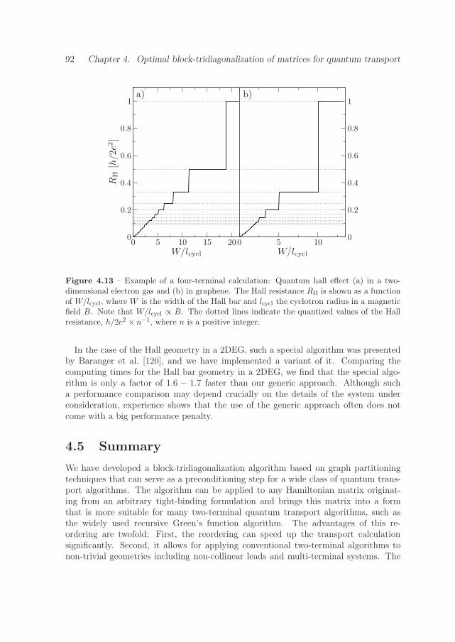
92 Chapter 4. Optimal block-tridiagonalization of matrices for quantum transport
Figure 4.13 – Example of a four-terminal calculation: Quantum hall effect (a) in a two-dimensional electron gas and (b) in graphene. The Hall resistance RH is shown as a functionof W/lcycl, where W is the width of the Hall bar and lcycl the cyclotron radius in a magneticfield B. Note that W/lcycl ∝ B. The dotted lines indicate the quantized values of the Hallresistance, h/2e2 × n−1, where n is a positive integer.
In the case of the Hall geometry in a 2DEG, such a special algorithm was presentedby Baranger et al. [120], and we have implemented a variant of it. Comparing thecomputing times for the Hall bar geometry in a 2DEG, we find that the special algo-rithm is only a factor of 1.6 − 1.7 faster than our generic approach. Although sucha performance comparison may depend crucially on the details of the system underconsideration, experience shows that the use of the generic approach often does notcome with a big performance penalty.
4.5 Summary
We have developed a block-tridiagonalization algorithm based on graph partitioningtechniques that can serve as a preconditioning step for a wide class of quantum trans-port algorithms. The algorithm can be applied to any Hamiltonian matrix originat-ing from an arbitrary tight-binding formulation and brings this matrix into a formthat is more suitable for many two-terminal quantum transport algorithms, such asthe widely used recursive Green’s function algorithm. The advantages of this re-ordering are twofold: First, the reordering can speed up the transport calculationsignificantly. Second, it allows for applying conventional two-terminal algorithms tonon-trivial geometries including non-collinear leads and multi-terminal systems. The

4.5. Summary 93
block-tridiagonalization algorithm scales as O(Ngrid logNgrid), where Ngrid is the sizeof the Hamiltonian matrix, and thus induces only little additional overhead. We havedemonstrated the performance of the matrix reordering on representative examples,including transport in 2DEGs and graphene.
The framework set by the non-equilibrium Green’s function formalism in tight-binding representation, presented in Chapter 2, provides a clear pathway for numer-ical transport calculations. Together with the novel results of the last two chapters,namely the general expression for the surface Green’s function of the leads and theblock-tridiagonalization algorithm, it is then possible to develop a transport code ap-plicable to arbitrary tight-binding systems. This is possible, since both the calculationof the surface Green’s function and the block-tridiagonalization algorithm can operateas a black box, i.e. without the need for specifying external parameters other than thetight-binding Hamiltonian H . Such a generic transport code is desirable, as it min-imizes development time and increases code quality, as only a few basic, thoroughlytested transport routines are necessary.
The algorithms developed in this work have been implemented in a computer pro-gram, as a set of transport routines requiring only the input of the tight-binding Hamil-tonian H . Adapting this code to an arbitrary tight-binding models thus only consistsof appropriately setting up the matrix H . This has been done for the cases of a two-and three-dimensional effective mass model as well as for graphene, including the spindegree of freedom. In the remainder of this thesis we will employ this code to computespin transport properties in magnetic tunnel junctions and graphene nanoribbons.


Part II
Spintronics in graphene andmagnetic tunnel junctions


“The hype is bigger, because thephysics is richer”
Carlo Beenakker – The New York Times, April 10, 2007


Chapter 5
Magnetic field effects on tunnelinganisotropic magnetoresistance
5.1 Introduction
Amongst the various magnetoresistive phenomena, the giant magnetoresistance (GMR)[14, 15] and the tunneling magnetoresistance (TMR) effect [16–18] are probably themost prominent examples. In both cases, the resistance of two ferromagnetic layersseparated by a spacer layer was found to depend on the relative angle of the magne-tizations in the two ferromagnets. While this spacer is a metal in the GMR effect, itis an insulating material for the TMR effect. Although the basic experimental geome-tries are very similar in both cases, the underlying physics is quite different: diffusivetransport in the case of GMR, and quantum mechanical tunneling in the case of TMR.Both the GMR and the TMR effect are employed in various electronic devices, suchas read heads of hard disks or magnetic random access memory (MRAM) (for reviewssee Refs. [12, 13, 19]).
In recent years, several experiments have found that the resistance of a magnetictunnel junction (MTJ) may also depend on the absolute angle of the magnetization ina ferromagnet with respect to some crystallographic axis, in contrast to the conventionalGMR and TMR effects, where the resistance depends only on the relative angle betweenthe magnetizations in two ferromagnetic layers. Amongst those, the most striking areexperiments on MTJs with only a single ferromagnetic layer that nevertheless showa magnetoresistance effect, depending on the orientation of the magnetization in theferromagnet [47, 149]. This magnetoresistance effect is called tunneling anisotropicmagnetoresistance (TAMR) effect.
The TAMR effect was first observed in a (Ga,Mn)As/Al2O3/Au tunnel junction, fea-turing epitaxially grown magnetic semiconductor (Ga,Mn)As as the ferromagnetic elec-

100 Chapter 5. Magnetic field effects on tunneling anisotropic magnetoresistance
Figure 5.1 – (a) Schematic view of the magnetic tunnel junction in the experiments ofRefs. [47, 150]. (b) TAMR effect for different bias voltages (Vbias = +90meV: © ; Vbias =−90meV: �) and magnetic fields (black: B = 0.5T; red: B = 5T; blue: B = 10T) in aFe/GaAs/Au tunnel junction (from [150]).
trode, and an amorphous aluminum-oxide tunnel barrier [149]. The observed TAMRexhibited a four-fold anisotropy and was explained by an anisotropic density of statesdue to uniaxial strain in the magnetic semiconductor.
A qualitatively different TAMR effect was found in epitaxially grown Fe/GaAs/Autunnel junctions with a single-crystalline tunnel barrier [47, 150], showing a uniax-ial anisotropy in the magnetoresistance. The GaAs barrier was grown in the [001]-direction, as indicated in the schematic of the experiment in Fig. 5.1(a). The angulardependence of the TAMR effect can be quantified as
TAMR(φ) =R(φ)− R(0)
R(0), (5.1)
where R(φ) is the resistance of the tunnel junction, when the magnetization in Fe formsan angle φ with the [110]-direction, as indicated in Fig. 5.1(a). In the experiment, theTAMR was found to be periodic in φ, with a periodicity of π, as shown in Fig. 5.1(b).The TAMR effect shows both a peculiar bias as well as magnetic field dependence: Fordifferent bias voltages Vbias the TAMR changes in magnitude, and may also changesign. Moreover, the magnitude of the effect decreases with increasing magnetic field Bwhen the TAMR effect is positive, and it increases when the TAMR effect is negative(magnetic field increases from the black to the blue symbols in Fig. 5.1(b)).
Theoretically, the TAMR effect for the case of small magnetic fields can be ex-plained by the effects of spin-orbit interaction in the tunneling process [47, 151, 152].This theory assumes that the momentum parallel to the layers (in-plane momentum)is conserved during the tunneling process, as appropriate for epitaxially grown (in con-trast to amorphous) systems. The interference of Bychkov-Rashba spin-orbit coupling

5.2. Magnetic field dependence of TAMR 101
at the Fe/GaAs interface and Dresselhaus spin-orbit coupling within the GaAs-barrierthen leads to the observed uniaxial anisotropy of the magnetoresistance. The biasdependence of the TAMR is explained by a bias-dependent value of the interfacialBychkov-Rashba spin-orbit parameter. However, up to now, a theoretical explanationof the magnetic field dependence of the TAMR is still missing. Such an explanation isthe objective of this chapter.
To this end, the chapter is organized as follows: First, we extend the theoreticalmodel of Refs. [47, 151, 152] to include the orbital effects of a magnetic field B. Theresulting model is then solved numerically and compared to experimental data. Finally,we develop a qualitative model for the B-field dependence of the TAMR, reproducingall characteristic features of the experiment.
5.2 Magnetic field dependence of TAMR
5.2.1 Model
Within the theoretical model of the TAMR effect, the Hamiltonian reads [47, 151, 152]
H = H0 +HD +HBR , (5.2)
where
H0 =1
2p
1
m(z)p + V (z)− Δ(z)
2n · σ . (5.3)
Here, p = −i�∇, and the coordinate system was chosen such that the z-direction isin the growth direction of the MTJ, as indicated in Fig. 5.1(a). m(z) is the effectivemass, with m(z) = 0.067me inside the GaAs barrier, and m(z) ≈ me within the Feand Au layer, where me is the bare electron mass. V (z) is the conduction band profileand Δ(z) the spin splitting. We neglect the Zeeman splitting in the barrier and thenon-magnetic electrode, as these are much smaller than any other energy scale in thesystem, and only keep the spin splitting due to the magnetization in the ferromagnet.The direction of this magnetization is given by
n =
⎛⎝cos θsin θ
0
⎞⎠ , (5.4)
where θ is the angle with respect to the x-axis. The experimentally used angle φ andθ are related through
φ = θ +π
4, (5.5)
as seen from the sketch in Fig. 5.1(a). σ is the vector of Pauli matrices. The shape of theconduction band offset resulting from this model is shown schematically in Fig. 5.2(a).The barrier height is approximately given by half the GaAs band gap, so that Vbar ≈0.75 eV. In addition, the Fermi wave vectors within Fe are k↑F,Fe = 1.05× 10¹⁰ m−1 and

102 Chapter 5. Magnetic field effects on tunneling anisotropic magnetoresistance
Figure 5.2 – (a) Schematic depiction of the conduction band profile for spin up (red solidline) and spin down (blue dashed line) for the theoretical model of the Fe/GaAs/Au tun-nel junction. (b) Comparison between the TAMR calculated numerically from the finitedifference approximation with a0 = 0.01 nm (black solid line) and from an approximate an-alytical expression [152] (red dashed line). The Bychkov-Rashba parameter was chosen asα = 25 eV A2.
k↓F,Fe = 0.44 × 10¹⁰ m−1 for spin up and down, respectively. Inside the Au layer, theFermi wave vector is given as kF,Au = 1.2× 10¹⁰ m−1.
HD and HBR describe the Dresselhaus and Bychkov-Rashba spin-orbit coupling, re-spectively. Here
HD =1
�(σx px − σy py)
∂
∂z
(γ(z)
∂
∂z
), (5.6)
where the Dresselhaus parameter is γ ≈ 24 eV A3
within the GaAs barrier and γ = 0outside. The Bychkov-Rashba spin-orbit coupling is only relevant at the Fe/GaAsinterface (which exhibits a broken inversion symmetry) and the Hamiltonian is givenas
HBR =1
�α (σx py − σy px) δ(z − zl) , (5.7)
where zl is the position of the left interface. In contrast to the Dresselhaus parameterγ which is a bulk property, the interface Bychkov-Rashba parameter is not known.Instead, α is used as a fitting parameter to describe the TAMR at a given bias volt-age Vbias, hence resulting in a bias-dependent Bychkov-Rashba parameter α(Vbias). Asummary of the material parameters used in the model is given in Table 5.1. Further-more, in the remainder of this chapter we fix the barrier width d = 8 nm, as in theexperiments.
In order to include the orbital effects of a magnetic field B into this model, we first

5.2. Magnetic field dependence of TAMR 103
mGaAs mFe mAu Vbar k↑F,Fe k↓F,Fe kF,Au γGaAs
0.067 me me me 0.75 eV 1.05×10¹⁰ m−1 0.44×10¹⁰ m−1 1.2×10¹⁰ m−1 24 eV A3
Table 5.1 – Summary of the material parameters of the theoretical model for theFe/GaAs/Au tunnel junction (from Refs. [13, 47, 151]).
note that the magnetic field is antiparallel to n, so that1
B =
⎛⎝−B cos θ−B sin θ
0
⎞⎠ . (5.8)
We then choose the vector potential such that
A(z) =
⎛⎝−B sin θ zB cos θ z
0
⎞⎠ , (5.9)
where B = ∇ × A. The magnetic field then enters the Hamiltonian via minimalcoupling
p→ p + eA(z) . (5.10)
This substitution must be done for any momentum operator in the Hamiltonian, in-cluding the spin-orbit terms.
In the chosen gauge, the vector potential in Eq. (5.9) only depends on the longitudinalcoordinate z. Hence, the Hamiltonian is still translationally invariant in x and y-direction, and Bloch’s theorem applies. Therefore, the full wave function can be writtenas
ϕ(x) = ei(kxx+kyy)ϕ(z) , (5.11)
and the Schrodinger equation for the Hamiltonian H reduces to a one-dimensionaldifferential equation for ϕ(z). The transverse wave vector k|| = (kx, ky)
t is a goodquantum number, as in the case without magnetic field.
At this point it should be emphasized that the conservation of k|| during the tunnelingprocess is not in contradiction to the cyclotron effects expected from a magnetic field.In fact, physically observable quantities, such as the electron velocity v|| = 1
m(�k|| +
eA||(z)) do show the transverse acceleration expected from the Lorentz force2.
1 Magnetic moments μ align parallel to the magnetic field B, but the magnetic moment of an electronis antiparallel to its spin: μe = − e
2meg �
2σ, where g ≈ 2 is the gyromagnetic factor of the electron.2 For further discussion on the difference between canonical and mechanical momentum, see, for
example, Ref. [153, App. III]

104 Chapter 5. Magnetic field effects on tunneling anisotropic magnetoresistance
The choice of gauge in Eq. (5.9) also comes with a disadvantage: It is not possibleto include a magnetic field in the contacts3. In practice, we therefore switch off themagnetic field after some distance away from the barrier. This is a good approximation,as the effects of the magnetic field are expected to be strongest in the barrier andnegligible in the metallic contacts: The cyclotron radius lcycl = pF/eB [111] takes thevalues lcycl ≈ 700 nm in Fe and lcycl ≈ 800 nm in Au, much larger than any relevantlength scale in the problem. Indeed, we find that the numerical results are insensitiveto the exact position where the magnetic field is switched off.
In order to solve the Hamiltonian (5.2) including a magnetic field numerically, weemploy the finite difference approximation that yields a tight-binding description of thesystem (for details, see Appendix F). The Delta function in Eq. (5.7) is approximatedby a step function of width 2a0, centered at the Fe/GaAs interface. Here, a0 is thelattice spacing of the discretization. In order to compare our numerical results with theprevious analytical results of Refs. [47, 151, 152], we choose a very fine lattice spacinga0 = 0.01 nm, to obtain a good approximation for the Delta function in Eq. (5.7).4
For a given k||, the transmission probability T (E,k||) at energy E can then be calcu-lated using the numerical techniques developed in Part I. Then, the total conductanceis given as
G(φ) =S
(2π)2
∫dk|| T (E,k||) , (5.12)
where S is the cross-section area of the magnetic tunnel junction. Note that the finitedifference approximation as presented in Appendix F is not restricted to situationswhere k|| is conserved, but can be also applied to disordered systems [155]. In termsof conductances, the TAMR value is given as
TAMR(φ) =R(φ)− R(0)
R(0)=G(0)−G(φ)
G(φ). (5.13)
In Fig. 5.2(b) we show a comparison of the TAMR effect without magnetic field calcu-lated both numerically and from an approximate analytical expression [152]. Given thefact that the analytical expression is only approximate, we find a very good agreementbetween the numerical and analytical results5 confirming the validity of the numericalprocedure.
3 First of all, scattering states can only be defined if the vector potential is parallel to the directionof the lead [154]. Second, also the method to calculate the surface Green’s function presented inChapter 3 is based on translational invariance along the lead direction.
4 For the description of the experiment it is not necessary to choose such a fine lattice spacing. Infact, no length scales smaller than the inter-atomic distance should play a role. However, the valueof the Bychkov-Rashba parameter α depends on the width 2a0 of the step function mimicking theDelta function of Eq. (5.7); hence a fine lattice spacing is needed to compare with the previousanalytical results.
5 When comparing results from this thesis and previous work, note that Refs. [47, 151] used a differentsign convention for α.

5.2. Magnetic field dependence of TAMR 105
5.2.2 Numerical results
We now compare the results of numerical simulations on the magnetic field dependenceof the TAMR effect with the corresponding experimental data. For this, we fit theparameter α at B = 0.5 T for every value of the bias voltage Vbias to the experimentaldata. In doing so, we obtain the bias voltage dependence of α = α(Vbias), as inRefs. [47, 151]. The magnetic field dependence can then be calculated without fittingany further parameter.
In Fig. 5.3(a) we show the angular dependence of the TAMR effect for differentvalues of the bias voltage and magnetic field. The numerical simulations show thesame trend as the experiment: The TAMR effect decreases with increasing B, whenthe effect is positive, and it increases, when the effect is negative. Furthermore, thenumerical calculations reproduce the experimentally found change with magnetic fieldwithin a factor of 1.5 − 2. This is an especially satisfying agreement, given the factthat the magnetic field dependence is calculated without fitting any parameter.
In order to quantify the magnetic field dependence of the magnitude of the TAMReffect, we show TAMR(90◦) as a function of the magnetic field B in Fig. 5.3(b). Inthe experiment, we find that TAMR(90◦) changes linearly with B. Moreover, the slopeof this change is approximately independent of the bias voltage Vbias. Both of thesecharacteristic features are also found in the numerical simulations. As before, thenumerical results underestimate the slope of the magnetic field dependence only by afactor of 1.5− 2.
Up to now, detailed experimental data on the B-field dependence of TAMR(90◦) isonly available up to 5 T. From the magnetic field dependence of single TAMR curvesas shown in Fig. 5.3(a), it seems that TAMR(90◦) may change faster than linear in Bfor B > 5 T, although this is hard to decide from only a few points. In contrast, thenumerical simulations result in a linear B-dependence also for fields up to 10 T. Forlarge fields, other terms than those considered in Eq. (5.2) may become important [13].In any case, the discussion of this point should be postponed until further experimentaldata is available.
The numerical results of this section show that the orbital effects of a magnetic fieldare enough to reproduce the characteristic features of the magnetic field dependencein the experiment. In order to understand the underlying physical mechanisms of thiseffect, we develop a qualitative model of the B-field dependence of the TAMR effect inthe next section.
5.2.3 A qualitative picture
In order to develop a qualitative model for the magnetic field dependence of the TAMR,we extend the phenomenological model of Refs. [13, 151] to include finite magneticfields.
The transmission probability can be written as a perturbative expansion in the spin-

106 Chapter 5. Magnetic field effects on tunneling anisotropic magnetoresistance
Figure 5.3 – (a) Angular dependence of the TAMR effect as found in the experiment(left panel, from [150]) and from numerical simulations (right panel). Data is shown forVbias = +90meV (experiment: ©; theory: α = 25.1 eV A2, solid lines) and Vbias = −90meV(experiment: �; theory: α = −25 eV A2, dashed lines), as well as different magnetic fields:B = 0.5T (black), B = 5T (red), and B = 10T (blue). (b) TAMR(90◦) as a function ofmagnetic field in the experiment (left panel, from [48]) and from numerical simulations (rightpanel). Data is shown for Vbias = +135meV (α = 29.3 eV A2, black), Vbias = +90meV(α = 24.3 eV A2, red), Vbias = +50meV (α = 10.5 eV A2, blue), Vbias = −50meV(α = −33.4 eV A2, green), and Vbias = −90meV (α = −30.8 eV A2, violet).

5.2. Magnetic field dependence of TAMR 107
orbit coupling [13, 151],
T (E,k||) = T (0)(E, k||)+T (1)(E, k||)n ·w(k||)+T (2)(E, k||)(n ·w(k||)
)2+ . . . , (5.14)
where
w(k||) =
⎛⎝ αky + γkx
−αkx − γky
0
⎞⎠ (5.15)
is an effective spin-orbit field, obtained by averaging the spin-orbit field Beff(z), HSO =HD + HBR = Beff(z) · σ over the unperturbed states of the system, i.e. in the ab-sence of spin-orbit coupling. The effective Bychkov-Rashba and Dresselhaus parame-ters α = αfα(k||) and γ = γfγ(k||) are functions of k|| = |k||| only, as are the expansioncoefficients T (n)(E, k||). Note that the T (n)(E, k||) cannot be interpreted as transmis-sion probabilities individually—for example, being expansion coefficients, T (n)(E, k||)may very well be negative.
As before, the total transmission is obtained by integrating over all transverse wavevectors,
T = T (0) + T (1) + T (2) + . . . , (5.16)
where T (n) =⟨T (n)(E, k||)(n ·w(k||))n
⟩k|| and 〈. . . 〉k|| = 1
(2π)2
∫dk|| . . . . In principle,
the integration over transverse wave vectors must be restricted to values within theFermi sphere. However, in a tunnel junction the transmission probability is suppressedexponentially for increasing k|| (transmission is highest for perpendicular incidence,i.e. k|| = 0), and hence we can extend the k||-integration to infinity. To second order inthe spin-orbit coupling, the conductance of the magnetic tunnel junction is then foundas
G(φ) = G(0) + a(2)0 + a
(2)1 αγ cos(2φ) , (5.17)
where G(0), a(2)0 , and a
(2)1 are coefficients obtained by taking the respective k||-integra-
tions for the zeroth- and second-order term in Eq. (5.14) (for details, see Ref. [13]). Inparticular, the coefficient a
(2)1 does not depend on the spin-orbit parameters α and γ.
The linear term in Eq. (5.14) vanishes exactly upon integration, as w(−k||) = −w(k||).After reviewing the phenomenological model for B = 0, we now turn to the case
of finite magnetic field B. In this situation, we can still expand the transmissionprobability with respect to the spin-orbit coupling, albeit with different expansioncoefficients and a different effective spin-orbit field:
TB(E,k||) = T(0)B (E,k||) + T
(1)B (E,k||)n ·wB(k||) + T
(2)B (E,k||)
(n ·wB(k||)
)2+ . . . .
(5.18)In the following we will derive approximate relations valid to linear order in B betweenthe expansion coefficients T
(n)B and the effective spin-orbit field wB to their counterparts
for B = 0.First, we consider the orbital effects of the magnetic field in the kinetic energy
term of the Hamiltonian, and neglect the spin-orbit coupling. The kinetic part of the

108 Chapter 5. Magnetic field effects on tunneling anisotropic magnetoresistance
Hamiltonian including a magnetic field reads
Hkin =�
2
2m
((kx −
eB
�sin θ z
)2
+
(ky +
eB
�cos θ z
)2
− ∂2
∂z2
), (5.19)
where for the sake of argument we neglect the spatial dependence of the effective massm. The effect of the magnetic field is two-fold: First, the maximum of the transmissionprobability is shifted with respect to k|| = 0. Instead, the maximum of TB(E,k||) isexpected at k||,0 with⟨(
kx,0 −eB
�sin θ z
)2⟩
= 0 and
⟨(ky,0 +
eB
�cos θ z
)2⟩
= 0 , (5.20)
where 〈. . . 〉 denotes an average over a quantum mechanical state. Hence, k||,0 can bewritten as
kx,0 = +b1B sin θ (5.21a)
ky,0 = −b1B cos θ , (5.21b)
where b1 is a coefficient that depends on both 〈z〉 and 〈z2〉. This shift can be regardedas the effect of the Lorentz force on the electrons. Second, the overall transmissionprobability decreases [156]. However, this effect is quadratic in B and will thus beneglected in the following. These considerations motivate the approximation
T(n)B (E,k||) ≈ T (n)
(E,
√(kx − b1B sin θ)2 + (ky + b1B cos θ)2
). (5.22)
In addition to the transmission probability, also the effective spin-orbit field is shiftedby the orbital terms from the magnetic field in Eqs. (5.6) and (5.7). The spin-orbitterms including a magnetic field read
HSO =α
(σx
(ky +
eB
�cos θ z
)− σy
(kx −
eB
�sin θ z
))δ(z − zl)+
γ
(σx
(kx −
eB
�sin θ z
)− σy
(ky +
eB
�cos θ z
))∂
∂z
(γ(z)
∂
∂z
), (5.23)
and therefore the effective spin-orbit field is given as
wB(k||) ≈ w(kx − b2B sin θ, ky + b2B cos θ) , (5.24)
where b2 is a coefficient that only depends on 〈z〉, as the spin-orbit terms only containlinear momenta in the transverse directions. Thus, in general we can expect b1 �= b2.
With the approximations (5.22) and (5.24) we can now evaluate the total transmis-sion. Since the zeroth order term is to first order only shifted by the magnetic field,we obtain the same result as in the case without magnetic field after integration:⟨
T 0B(E,k||)
⟩k||≈ T (0) (5.25)

5.2. Magnetic field dependence of TAMR 109
Figure 5.4 – (a) Schematic picture of the influence of the magnetic field: The Fermi sphere(or, more precisely, the maximum of the transmission probability) is shifted with respect tothe effective spin-orbit field w(k||). (b) Magnetic field dependence of TAMR(90◦) when themagnetic vector potential is only included in the kinetic term (red dashed line), only in thespin-orbit term (blue dash-dotted line), or in both terms (black solid line).
The term linear in the spin-orbit coupling evaluates to⟨T 1
B(E,k||)n ·wB(k||)⟩k||
≈ 1
(2π)2
∫dk||T (1)(E, k||) n ·w(kx + (b1 − b2)B sin θ, ky − (b1 − b2)B cos θ)
=1
(2π)2
∫dk||T (1)(E, k||) B(b1 − b2)(
−α cos2 θ + γ sin θ cos θ − α sin2 θ + γ cos θ sin θ)
= (b1 − b2)B(⟨T (1)(E, k||)fγ(k||)
⟩γ sin(2θ)−
⟨T (1)(E, k||)fα(k||)
⟩α). (5.26)
In the second line we used the coordinate substitution kx → kx + b1B sin θ and ky →ky − b1B cos θ, and in the third line we made use of the fact that terms linear in kx orky vanish upon integration.
Hence, we find that the linear term, that vanished in the case without a magneticfield, gives a finite contribution for B �= 0. This is due to the fact that the Fermi sphereis shifted by the Lorentz force. In particular, the effective spin-orbit field is shiftedwith respect to the center of the transmission maximum, as sketched in Fig. 5.4(a).In addition, we find a different angular dependence for the Bychkov-Rashba and theDresselhaus spin-orbit coupling. This is due to different symmetries of the spin-orbitfields: The Bychkov-Rashba field exhibits a rotational symmetry [13] and thus leadsto an angular-independent term in Eq. (5.26), whereas the Dresselhaus field does not,and hence leads to a angular dependence.
Finally, in addition to the original contribution for B = 0, the second-order term

110 Chapter 5. Magnetic field effects on tunneling anisotropic magnetoresistance
in the spin-orbit coupling also contains terms quadratic in B, due to the shift of theFermi sphere. As before, we neglect these terms and approximate⟨
T 2B(E,k||)
⟩k||≈ T (2) . (5.27)
Hence, the conductance of the magnetic tunnel junction in a magnetic field B takesthe form
GB(φ) = G(0) + a(2)0 + a
(1)2 αB + (a
(2)1 αγ − a
(1)1 γB) cos(2φ) , (5.28)
where the coefficients
a(1)1 = − Se2
(2π)2h〈T (1)(E, k||)fγ(k||)〉(b1 − b2) (5.29a)
a(1)2 = − Se2
(2π)2h〈T (1)(E, k||)fα(k||)〉(b1 − b2) (5.29b)
do not depend on the spin-orbit parameters. The TAMR then evaluates to
TAMR(φ) ≈ GB(0)−GB(φ)
G(0)∝ (a
(2)1 αγ − a
(1)1 γB)(1− cos(2φ)) . (5.30)
This equation gives a qualitative explanation of all characteristic features observed inthe experiment: First, it reproduces the linear change in the TAMR with magneticfield. Second, the slope of this change is independent of the bias voltage, as it onlydepends on the (bulk) Dresselhaus parameter. Thus, all the experimentally observedfeatures can be explained with the orbital effects caused by the magnetic field.
From the numerical results we can deduce that a(2)1 , a
(1)1 > 0. In addition, the
numerical results also confirm that a(1)1 contains a factor (b1− b2), i.e. opposing contri-
butions from the orbital effects in the kinetic energy and in the spin-orbit coupling. InFig. 5.4(b) we show the magnetic field dependence of TAMR(90◦) when the magneticvector potential is included only in the kinetic term (dashed line), only in the spin-orbitterms (dash-dotted line) and in both terms (solid line). When the magnetic field is onlyincluded in one term, we find a large change of the TAMR effect with magnetic field,however with opposite signs. When the vector potential is included in both the kineticand the spin-orbit term, the contributions cancel to a large degree, leaving only a smalleffect. These numerical findings support the phenomenological model developed in thissection.
Finally, it should be mentioned that although the magnetic field dependence of theTAMR (5.30) only depends on the Dresselhaus parameter γ, the conductance (5.28)also contains a B-dependent contribution from the Bychkov-Rashba parameter α. Thisterm leads to a bias-voltage dependent linear slope in the magnetic field dependence ofthe conductance, in addition to the usual quadratic dependence [156]. Hence, it wouldbe of great interest if such a dependence was indeed observed in the experiments.

5.3. Summary 111
5.3 Summary
In this chapter we have studied the magnetic field dependence of the TAMR effect inepitaxially grown Fe/GaAs/Au tunnel junctions. For this, we have extended the modelused in previous works [47, 151, 152], which explained the TAMR effect through thespin-orbit coupling in the GaAs barrier, to include the orbital effects of a magneticfield. No additional fitting parameters were introduced in this step.
The observed magnetic field dependence—linear change in the TAMR with B anda bias-independent slope—could be explained both from the numerical simulationsand a phenomenological model, where the orbital effects of the magnetic field wereincluded as a shift of the Fermi sphere. In particular, the phenomenological modelpredicts that the slope of the TAMR change for a magnetic field B depends onlyon the (bulk) Dresselhaus spin-orbit parameter, and is hence bias-independent. Thisand other predictions from the phenomenological model are reproduced in numericalsimulations, supporting its validity.
The TAMR effect in Fe/GaAs/Au tunnel junctions has been attributed to the effectsof spin-orbit coupling in the GaAs barrier [47, 151, 152]. Including orbital effects intothis model, we could explain the experimentally observed magnetic field dependencewithout any additional fitting parameters. This strongly supports the initial assumptionthat indeed spin-orbit coupling is the reason for the TAMR effect.


Chapter 6
The graphene edge state
6.1 Introduction
Graphene is a two-dimensional crystal of carbon atoms. Since its experimental dis-covery in 2004 [29], graphene has attracted a tremendous amount of interest (for re-views, see [31, 35, 157]). On the one hand, this is due to the fact that charge carriersin graphene obey an effective equation that mimics relativistic dynamics, leading tomany unique physical properties, such as the odd-integer quantum Hall effect [32] thateven prevails at room temperature [33], or Klein tunneling [34]. On the other hand,graphene is also a very promising material for electronics, because of its high mobility[36, 37], even at room-temperature [29], paving the road to ballistic transistors [31].
However, since (bulk) graphene does not feature a band gap, conventional transistoraction is difficult to achieve. In contrast, graphene nanoribbons, strips of finite widthcut from a graphene sheet, exhibit a finite band gap scaling with the nanoribbonwidth [158–160], and, as a consequence, room-temperature transistor action has beendemonstrated [161]. The origin of this band gap is still under discussion [162–166].
Whereas the edges of graphene nanoribbons were not well-controlled in the earlyexperiments, recent progress in fabrication has shown that controlled manufacturingof nanoribbons with atomically defined edges seems within experimental reach in thenear future [160, 167, 168]. From a theoretical point of view, the electronic propertiesof nanoribbons are expected to depend crucially on the structure of the edge [169].In particular, a zigzag or zigzag-like edge is expected to support a state localized atthe graphene edge [169–171]. This edge state has been observed experimentally usingscanning tunneling (STM) microscopy for a graphene edge on the surface of graphite1
[172–174]. Due to electron-electron interactions, the edge state is expected to exhibit
1 Up to now, a direct experimental confirmation of the edge state for exfoliated or epitaxially growngraphene is still missing.

114 Chapter 6. The graphene edge state
Figure 6.1 – (a) Lattice structure of graphene. (b) First Brillouin zone of graphene.
magnetism [170, 175, 176]. This magnetism can be used in edge state based spintronicsthat we present in Chapter 7.
On the theoretical side, the transport in situations, where the edge state is impor-tant, is almost exclusively studied in nearest-neighbor tight-binding approximation (forexample, see Refs. [162, 165, 166, 177–181]). However, it has already been shown thatthe effects of next-nearest neighbor hopping on the edge state are significant in termsof the band structure [182, 183]. In addition, edge magnetism also changes the edgestate related band structure considerably [164, 176].
Therefore, it is the intent of this chapter to study the fundamental properties ofedge state transport in graphene. Doing so, we show that the paradigm model oftransport in graphene, the nearest-neighbor tight-binding model, is not suitable forstudying edge state transport: The results of edge transport in nearest-neighbor tight-binding approximation change fundamentally upon exponentially small corrections tothis model.
To this end, the chapter is organized as follows: We begin by summarizing the mainresults of the tight-binding model of graphene employed in this work (for a completediscussion, see Appendix G). In addition, we review symmetries of the graphene Hamil-tonian, that impose certain restrictions on the graphene wave function. These resultsare then applied to characterize the properties of the edge state for different approx-imations to the graphene Hamiltonian. Finally, we discuss extensively the transportproperties of the graphene edge state when corrections to the nearest-neighbor tight-binding approximation are included.
6.2 Fundamentals of graphene
6.2.1 Graphene Hamiltonian
The electronic structure of graphene is usually described in terms of a tight-bindingmodel, that is discussed extensively in Appendix G. Here, we merely summarize themain results.

6.2. Fundamentals of graphene 115
Graphene is a two-dimensional sheet of carbon atoms, arranged in a honeycombnetwork, as shown in Fig. 6.1(a). The honeycomb network is not a primitive Bravaislattice, but is generated by a triangular lattice with two basis atoms. These basis atomsare labeled A and B, respectively, and the triangular lattice constant is denoted as a.
In single-orbital tight-binding approximation, the graphene Hamiltonian reads
H =∑
i,α,j,β
tiαjβ |i, α〉 〈j, β| . (6.1)
Here, |i, α〉 denotes the orbital at lattice site Ri +dα, where Ri is a (triangular) latticevector and dα the relative position of atom α = A,B within the unit cell. We considermatrix elements up to next-nearest neighbors, so that
tiαjβ =
⎧⎪⎪⎪⎨⎪⎪⎪⎩Vi +Mi if i = j, α = β = A
Vi −Mi if i = j, α = β = B
−t if i, α and j, β are nearest neighbors,
−t′ if i, α and j, β are next-nearest neighbors.
(6.2)
Here Vi is a potential that has the same value on both sublattices, andMi is a staggeredpotential, i.e. has opposite sign on atom A and B, respectively. The numerical valuesof the hopping parameter are chosen as t = 2.7 eV and t′ = 0.1t [183, 184].
In the case of an infinite graphene sheet and constant potentials Vi = V0 andMi = M ,Bloch’s theorem holds and in k-space the Hamiltonian reads (Eq. (G.23))
H(k) =(V0 − 2t′
3∑l=1
cos(kδ′l))1−
(t
3∑l=1
cos(kδl))σx +
(t
3∑l=1
sin(kδl))σy +Mσz ,
(6.3)where σx,y,z are the Pauli matrices and δl (δ′l) the distance vectors between nearest(next-nearest) neighbors. Note that the two basis atoms in the unit cell give rise to awave function with two components, referring to sublattice A and B,
ϕ(j) =
(ϕA(j)ϕB(j)
)(6.4)
such that the Hamiltonian H(k) can be written as a 2× 2-matrix in Eq. (6.3).The wave vector k is defined within the first Brillouin zone of graphene that has
the shape of a hexagon, as shown in Fig. 6.1(b). Only two of the six corners of theBrillouin zone are unique, as always three corners are connected by a reciprocal latticevector. These two non-equivalent corners are called K and K ′-point, respectively. Herewe choose
Kτ =
(τ 4π
3a
0
)(6.5)
to represent the K (τ = +1, K = K+) and K ′-point (τ = −1, K′ = K−).

116 Chapter 6. The graphene edge state
In a system close to charge neutrality, the states at the Fermi energy EF have a wavevector close to theK andK ′-point. States close to K and K′ are said to be in theK andK ′-valley. In the low energy regime and for smoothly varying potentials, the particledynamics can be described by an effective Hamiltonian in each valley (Eq. (G.36)),
Hτ = −i�vF (τ∂xσx + ∂yσ
y) + V (x) +M(x) σz , (6.6)
where HK = H+ is the effective Hamiltonian for the K-valley and HK ′ = H− forthe K ′-valley. Here, V (x) and M(x) are a smoothly varying potential and staggeredpotential, respectively, and vF =
√3ta/2 ≈ 106 m/s is the Fermi velocity. Again, the
two sublattices give rise to a two-component envelope wave function
ϕ(x) =
(ϕA(x)ϕB(x)
), (6.7)
and the Pauli matrices σx,y,z act within this sublattice space.The effective Hamiltonian in Eq. (6.6) is equivalent to a Dirac Hamiltonian in two
spatial dimensions, albeit with an “effective speed of light” vF. As a consequence,the low-energy spectrum of graphene is linear close to the K and K ′-point. Thisgives rise to a cone-like shape of the band structure in the K and K ′-valley, that iscommonly referred to as Dirac cone. Furthermore, the two-component wave function(6.7) behaves like a spinor under transformations, and the sublattice degree of freedomis thus referred to as pseudospin.
The envelope wave function (6.7) and the tight-binding wave function (6.4) are con-nected through (Eq. (G.38))
ϕα(j) = eiK(Rj+dα) ϕα(Rj + dα) + eiK′(Rj+dα) ϕ′α(Rj + dα) , (6.8)
where ϕα(x) and ϕ′α(x) are the envelope wave functions in the K and K ′-valley, re-spectively.
6.2.2 Symmetries of the graphene Hamiltonian
We will now review some important symmetries of the graphene Hamiltonian, in par-ticular particle-hole symmetries. If the Hamiltonian H is particle-hole symmetric, thereis a transformation P such that
P†HP = −H . (6.9)
Then, if ϕ is an eigenstate of H with energy E, Hϕ = Eϕ, Pϕ is an eigenstate withenergy −E, HPϕ = −EPϕ. Thus, the energy spectrum is symmetric with respect toE = 0 and every “particle” wave function ϕ with positive energy has a “hole” partnerPϕ with negative energy.
Writing the tight-binding Hamiltonian in terms of Pauli matrices as in Eq. (6.3) hasthe advantage that we can treat it on equal footing with the effective Dirac Hamiltonian

6.2. Fundamentals of graphene 117
(6.6). The symmetries and their consequences considered below are thus valid for boththe tight-binding and the effective Hamiltonian.
The Hamiltonian is particle-hole symmetric under the unitary transformation
Pz = σz , (6.10)
if it contains only terms proportional to σx or σy. That is, Pz is a particle-hole trans-formation if the Hamiltonian does not include potentials2 V (x) and M(x) and, in thecase of the tight-binding Hamiltonian, only includes nearest-neighbor hopping3.
In order to exist also in a system of finite extent, the particle-hole symmetry mustadditionally be compatible with the boundary conditions [171]. In a finite graphenepatch, the wave function must vanish on a set of missing atoms, as discussed in SectionG.3.2. Since Pz does not mix sublattice A and B, it is compatible with any boundary.
The particle-hole transformation Pz is especially important, as it also has conse-quences for the occupation probabilities of the two sublattices [185]. Note that 1
2(1±σz)
is a projection operator onto the wave function of sublattice A and B, respectively.From this projection operator we obtain the following expression for an eigenstate ϕwith energy E, provided that {Pz, H} = 0:
〈ϕ| 12
(1 + σz)H1
2(1− σz) |ϕ〉 = 〈ϕ| 1
2(1 + σz)
1
2(1 + σz)H |ϕ〉
=E
∫dx |ϕA(x)|2 (6.11)
Commuting the Hamiltonian H to the left we also obtain
〈ϕ| 12
(1 + σz)H1
2(1− σz) |ϕ〉 = E
∫dx |ϕB(x)|2 (6.12)
and thus, combining Eqs. (6.11) and (6.12),∫dx |ϕA(x)|2 =
∫dx |ϕB(x)|2 for E �= 0. (6.13)
Hence, if the Hamiltonian is particle-hole symmetric under Pz, every eigenstate withenergy E �= 0 occupies sublattice A and B with equal probability.Pz is not the only particle-hole symmetry in the system. For example, the effective
Hamiltonian is particle-hole symmetric under the antiunitary transformation [186]
Px = Cσx , (6.14)
2 Note that a constant potential V (x) = V0 only leads to an overall energy shift; as such, it does notbreak particle-hole symmetry.
3 In the low-energy regime, the next-nearest neighbor hopping does not play a role (see Section G.2.3).Thus, close to the Dirac point, the spectrum is still approximately particle-hole symmetric, evenif next-nearest neighbor hopping is included. However, this is not true anymore, if edge states arepresent (see Section 6.3.4).

118 Chapter 6. The graphene edge state
σx, σy M(x)σz V (x)1 t′ �= 0
particle-hole symmetry yes yesa no no∫dx|ϕA(x)|2 =
∫dx|ϕA(x)|2 yesb no no no
Table 6.1 – Summary of which terms in the graphene Hamiltonian break particle-hole sym-metry, and which terms imply equal occupation probability on sublattice A and B.a In bulk; for armchair boundaries; for zigzag boundaries provided that there is an additional
symmetry connecting zigzag edges of the opposite kind (such as in nanoribbons).b For E �= 0.
where C denotes complex conjugation. The tight-binding Hamiltonian, in turn, isparticle-hole symmetric under
Py = Cσy . (6.15)
Both Px and Py are particle-hole transformations if the respective Hamiltonian onlycontains terms proportional to σx, σy and σz, i.e. including a staggered potential.
However, unlike Pz, these particle-hole symmetries interchange sublattice A and Band are thus only compatible with boundary conditions that involve both sublattices onequal footing, such as armchair boundary conditions. In particular, a zigzag edge breaksthese particle hole symmetries—unless there is an additional symmetry connectingdifferent zigzag edges as in a zigzag nanoribbon. Still, even if Px,y is a particle-holetransformation, it does not give rise to a relation for the occupation probability of thetwo sublattices.
The findings of this section are summarized in Table 6.1.
6.3 Characterization of the edge state
6.3.1 Edge state at a single zigzag edge
Over the course of the next sections, we will examine the graphene edge state underdifferent conditions. Here, we start with the simplest situation, a half-infinite graphenesheet with a single zigzag edge in nearest-neighbor tight-binding approximation.
It has been known for some time that a zigzag edge in a honeycomb network supportsa state localized at the edge [96, 187], but it was Fujita that first noticed the physicalrelevance of this state [170]. As Fujita, we consider a half-infinite graphene sheet witha single zigzag edge in x-direction, as sketched in Fig. 6.2(a). In this situation, theoutermost atoms are all of sublattice B, and the wave function vanishes on the firstrow of missing A atoms.
The half-infinite graphene sheet can be understood as a repetition of unit cells oflength a, where the unit cell is given as a chain of carbon atoms, as indicated in black inFig. 6.2(a). We label atoms within this unit cell by (j, α), where j = 0, 1, 2, . . . increaseswhen moving away from the edge and α = A,B denotes the sublattice. Note that in

6.3. Characterization of the edge state 119
Figure 6.2 – (a) A half-infinite graphene sheet with a single zigzag edge in nearest-neighbortight-binding approximation. The unit cell of the system is indicated in black, and the firstrow of missing atoms is indicated by crosses. (b) The same situation within the effectiveDirac Hamiltonian.
our convention, the first missing atom has index (0,A). The unit cells themselves arelabeled with an index n, that increases with increasing x.
Because of translational symmetry in x-direction, we can write the wave function ofthe system in Bloch form,
ϕα(n, j) = φα(j)ei ka n , (6.16)
where k ∈ [−πa, π
a]. Within a unit cell, the atomic positions change by ±a
2in x-direction
when going from j to j + 1 or j − 1. In order to eliminate the phase associated withthis lateral displacement, it is convenient to define
φα(j) = φα(j) for j even, (6.17)
φα(j) = φα(j) e−ika/2 for j odd. (6.18)
Making use of the Bloch form (6.16) we can then write down the stationary Schrodingerequation Hϕ = Eϕ as a set of equations only involving φα(j):
E φA(j) = −t φB(j) + t e−γ φB(j − 1) (6.19)
E φB(j) = −t φA(j) + t e−γ φA(j + 1) , (6.20)
where we defined e−γ = −2 cos(ka/2). This set of equations is closed by the boundarycondition φA(0) = 0, so that
E φB(0) = −t φA(1) . (6.21)
It is easy to see that these equations have a solution for E = 0:
φA(j) = 0, φB(j) = e−γj . (6.22)

120 Chapter 6. The graphene edge state
This solution is normalizable—and thus represents a physical solution—if |e−γ| =|2 cos(ka/2)| < 1, i.e. −π
a≤ k < −2π
3aand 2π
3a< k < π
a. From
∞∑j=0
e−2γj =1
1− e−2γ(6.23)
we find the normalized solution
φA(j) = 0 φB(j) =√
1− e−2γ e−γj . (6.24)
This is the celebrated graphene edge state. Note that this state resides on a singlesublattice—since it is a zero-energy solution, Eq. (6.13) does not hold, although thenearest-neighbor tight-binding Hamiltonian is particle-hole symmetric with respect toPz.
The edge state is a solution that decays exponentially in the direction perpendicularto the edge. The perpendicular decay constant γ, and thus the perpendicular extensionof the edge state, depends uniquely on the lateral wave vector k, γ = γ(k). This isin contrast to an edge in an ordinary, semiconductor based two-dimensional electrongas, where the perpendicular and the lateral direction are decoupled. The edge stateis maximally localized for k = ±π
a, where it resides on the outermost atom only,
|φB(j)|2 =
{1 for j = 0
0 else,(6.25)
and extends through the whole system for k = ∓2π3a
(that is, at the K and K ′-point,respectively),
|φB(j)|2 = const. (6.26)
Close to the K-points, we find
γ = iπ −√
3a
2
(k ∓ 2π
3a
)+O
((k ∓ 2π
3a
)2), (6.27)
i.e. the perpendicular decay constant depends linearly on the lateral wave vector k.In contrast to the decay length, the energy of the edge state E(k) = 0 is a constant,
independent of k. Thus, the edge state is dispersionless, i.e. has zero group velocity. InFig. 6.3 we show a schematic picture of the band structure of a half-infinite graphenesheet including the edge state (for a discussion on how to project the two-dimensionalband structure of graphene into one dimension, see Section G.3.1). The edge stateband is perfectly flat and connects the two K-points.
After discussing the edge state within the tight-binding model, we now turn to theeffective Dirac Hamiltonian. Again, because of translational symmetry in x-direction,the wave function of the system can be written in Bloch form
ϕ(x) = φ(y) eiqx . (6.28)

6.3. Characterization of the edge state 121
Figure 6.3 – Schematic depiction of the edge state dispersion E(k), shown in red. The Diraccones are indicated in light grey.
Note that a wave vector in the effective Hamiltonian is always given with respect tothe K or K ′-point, as discussed in Section G.2.3. We will always denote such a relativewave vector by q, in order to distinguish it from a wave vector k in the tight-bindingmodel.
Using Eq. (6.28) in the effective Dirac Hamiltonian (6.6) we obtain a one-dimensionaldifferential equation for the transverse wave function
�vF (τq − ∂y)φB(y) = E φA(y) (6.29)
�vF (τq + ∂y)φA(y) = E φB(y) , (6.30)
where τ = +1 for the K-valley and τ = −1 for the K ′-valley. The boundary conditionfor a half-infinite graphene sheet as sketched in Fig. 6.2(b) is then
φA(0) = 0 . (6.31)
For E = 0, these equations have the solution
φA(y) = 0 φB = eτqy . (6.32)
This solution is normalizable, if τq < 0, i.e. for negative (positive) wave vectors q withrespect to the K(K ′)-point. Note that this is consistent with the tight-binding result,where k < −2π
3a(K-point) or k > 2π
3a(K ′-point). The normalized edge state solution
then reads
φ(y) =
(0√−2τq eτqy
). (6.33)
Thus, also within the effective Hamiltonian we find an edge state solution that decaysexponentially in the perpendicular direction. Again, the decay length depends on thelateral wave vector q. Furthermore, the perpendicular decay constant τq is in agreementwith the linear expansion of γ close to the K-points, Eq. (6.27).4 Thus, close to theK-points, the edge state is well-described by the effective Dirac Hamiltonian.
4 For this, note that the y-coordinate of the j-th atom is given by yj = j√
3a/2.

122 Chapter 6. The graphene edge state
Figure 6.4 – Comparison between the edge state solutions of the tight-binding (solid lines)and the effective Hamiltonian (dashed lines). (a) shows the probability density |φB(y)|2 fordifferent values of k, and (b) the wave functions φB(y) for k = −2.3/a as a function of thedistance y from the edge. In (b), we denote this distance as yj in order to emphasize that thevalues of the wave function are only given for fixed atom positions. In order to convenientlycompare the wave functions for different values of k, they have been normalized such thatφB(0) = 1.
In Fig. 6.4(a) we show a comparison between the edge state from the tight-bindingand the effective Hamiltonian for different values of k. As expected, close to the K-point, both solutions agree very well. Moving away from the K-point, the edge statefrom the effective Hamiltonian decays somewhat slower than the edge state withinthe tight-binding model. In fact, the tight-binding edge state solution is maximallylocalized for k = ±π
a, whereas the edge state solution in the effective Hamiltonian
is localized strongest for τq → −∞. The point of maximal localization, k = ±πa,
is located halfway between the K and K ′-points. Around this point, the validity ofthe effective Hamiltonian, that is an expansion around a single K-point, breaks down.Thus, it is not surprising that the effective Hamiltonian underestimates the strengthof the edge state decay, but as seen in Fig. 6.4, this deviation is small.
In addition to the exponential decay, the edge state also features a change in signfrom atom to atom, since e−γ < 0. In order to obtain such an oscillation on the scaleof the lattice from the smooth envelope wave functions of the effective Hamiltonian,we have to use Eq. (6.8) to relate the envelope wave functions to the tight-bindingsolution. For the case of the edge state, this is shown in Fig. 6.4(b), where we find agood agreement between both solutions.
Hence, the effective Dirac Hamiltonian describes the main features of the grapheneedge state rather well, but somewhat underestimates the strength of the decay. There-fore, when keeping in mind this limitation, the effective Hamiltonian can be appliedsuccessfully to study the edge state in more complex situations, when an analyticalsolution of the tight-binding model is not possible anymore.

6.3. Characterization of the edge state 123
Figure 6.5 – (a) A zigzag graphene nanoribbon and (b) its equivalent within the effectiveDirac Hamiltonian.
6.3.2 Edge state in a zigzag nanoribbon
We now turn to a system containing two parallel zigzag edges, i.e. a zigzag graphenenanoribbon. It is still possible to solve the tight-binding Hamiltonian in nearest-neighbor approximation analytically in this case [183]. However, the resulting ex-pressions are rather unwieldy. Thus, here we restrict the discussion to the effectiveDirac Hamiltonian in order to obtain the characteristic features of the edge state in ananoribbon.
Since the zigzag nanoribbon again has translational symmetry in x-direction, theeigenstates will have the Bloch form as given in Eq. (6.28). The boundary conditionsthen read
φA(0) = 0, φB(W ) = 0 , (6.34)
where W is the width of the nanoribbon (see Fig. 6.5). The problem of solving theeffective Dirac Hamiltonian (6.6) with these boundary conditions has been addressedin Refs. [53, 185]. The edge state solution is given as
φ(y) ∼=(
sinh (zy)sgn(E) sinh (z (W − y))
)(6.35)
where the decay constant z is real and obeys
q = −τ z
tanh (zW ). (6.36)
Again, τ = +1 for the K and τ = −1 for the K ′-valley. The edge state has theeigenenergy
E = ± z
sinh zW. (6.37)
The solution (6.35) is decaying exponentially in the perpendicular direction and canthus be called an edge state, if the transcendental equation (6.36) has a real solutionz. This is the case for τq < −1/W . Note that the critical value of q for obtainingan edge state solution has been shifted slightly with respect to the single edge, where

124 Chapter 6. The graphene edge state
Figure 6.6 – A zigzag nanoribbon in nearest-neighbor tight-binding approximation: (a) Theband structure of the zigzag nanoribbon. (b) Probability density profile of the edge stateacross the zigzag nanoribbon, for k = −2.4/a. The inset shows the same density profile on alogarithmic scale. The probability density for sublattice A is shown in red, for sublattice Bin black. In both (a) and (b) the nanoribbon had a width W = 64a/
√3.
τq < 0 was required for the existence of an edge state. For wide enough ribbons, thisdifference becomes negligible.
The state at q = −τ/W has z = 0 and connects edge state and bulk-like solutions,as does the q = 0 state for the single edge. However, unlike for the case of the singleedge, where φB(y) = const., this connecting state decreases linearly from one edge tothe other [53], as it must satisfy the boundary conditions at both edges.
For zW � 1, i.e. a very wide ribbon, or a strongly decaying state, from Eq. (6.36)we obtain z ≈ −τq and the eigenstate simplifies to
φ(y) ≈(eτq(W−y)
±eτqy
). (6.38)
In this limit, the edge state in the zigzag nanoribbon is given as two decaying exponen-tials at each edge, residing on opposite sublattices (the boundary conditions at bothedges are opposite to each other), reminiscent of the edge state at a single edge asdiscussed in the previous section. From Eq. (6.37) we find the energy of this state as
E ≈ ∓2τq eτqW . (6.39)
This energy is exponentially close to zero, since −τqW = zW � 1. Thus, we find twostates with an exponentially small, but finite energy splitting. There are two states,since the nanoribbon features two edges.
These states appear as two almost dispersionless bands in the band structure ofa zigzag nanoribbon as shown in Fig. 6.6(a), where we calculated numerically theband structure of a zigzag nanoribbon in nearest-neighbor tight-binding approximation.

6.3. Characterization of the edge state 125
Since the energy of these states is exponentially small, these bands appear to have thesame energy when plotted in a linear scale. However, there is always an exponentiallysmall, but finite energy splitting between these states at a given value of k, with theexception of the two zero-energy states at k = ±π
a. There the effective Dirac theory
breaks down, as seen in the previous section. Moving closer to the K-points, thesplitting becomes larger, until the edge states join the extended, bulk-like states inthe Dirac cones (see also Section G.3.1). The existence of this splitting has importantconsequences that we discuss below. Note that the edge state band merges smoothlyinto a band of bulk states: The states for τq > −1/W are no longer localized to theedge, but extend through the whole width of the ribbon.
In Fig. 6.6(b) we show the probability density profile of an edge state across thenanoribbon. For the chosen value of the wave vector k, the edge state is localizedto the edges, and resides on a single sublattice close to the edges, as expected fromEq. (6.38). The inset of Fig. 6.6(b) shows the probability density of the edge state ina logarithmic scale, where the exponential decay is more apparent. Close to the edges,we observe a small “kink” in the decay, as the state must also satisfy the boundarycondition on the opposite edge.
A picture like Fig. 6.6(b) might lead to the impression that the two edges in the zigzagnanoribbon carry two independent edge states. This is not true: Fig. 6.6(b) shows asingle eigenstate of the nanoribbon. The nanoribbon in nearest-neighbor tight-bindingapproximation is particle-hole symmetric under transformation with Pz, and thus everyeigenstate with nonzero energy must occupy both sublattices with equal probability,as discussed in Section 6.2.2. It is thus not possible to find an eigenstate with nonzeroenergy that resides at a single edge and a single sublattice only. Thus, any edge statewith k �= ±π
ais located with equal probability at both edges. Since the probability
densities at both edges arise from a single state, they are inevitably coupled: whateverhappens at one edge, will also influence the probability density at the other edge. Thismust be kept in mind when discussing the edge state in a zigzag nanoribbon5.
Note that the edge state solutions (6.35) and (6.38) are of the form(φA(y)
0
)±(
0φB(y)
), (6.40)
i.e. a “bonding” and “anti-bonding” linear combination of wave functions on a singlesublattice. Combining “bonding” and “anti-bonding” solutions, it is in fact possibleto construct a wave function localized at single edge only. However, since these stateshave positive and negative energy respectively, the resulting wave function is not aneigenstate of the system.
Within the effective Dirac Hamiltonian, the “bonding” (“anti-bonding”) solutionhas a positive (negative) energy. In order to obtain the lattice wave function fromthe envelope wave functions, we again have to employ (6.8). The lattice structure
5 In fact, calling this state “edge state” is already a possible source of confusion.

126 Chapter 6. The graphene edge state
of the zigzag nanoribbon then leads to a peculiar even-odd effect with respect to thenanoribbon width [188], that is of crucial importance in valleytronics [188, 189], butdoes not play a role in this work.
As seen in this section, due to the symmetries of the graphene Hamiltonian it is notpossible to find a state localized at a single edge in a zigzag nanoribbon in nearest-neighbor tight-binding approximation6. In the next sections we therefore examine thebehavior of the edge state including additional terms in the Hamiltonian that breakthis symmetry.
6.3.3 Effects of a staggered potential
We first consider the effect of a staggered potential M . In a half-infinite graphenesheet, the edge state resides on a single sublattice only. The staggered potential thensimply shifts the edge state energy by −M , if the edge state resides on sublattice B,and +M , if the edge state resides on sublattice A.
In a nanoribbon, the situation is more complex, as the edge state is in principlelocated at both edges and both sublattices, as discussed in the previous section. How-ever, since a staggered potential breaks the particle-hole symmetry Pz, the eigenstatesof the zigzag nanoribbon need not occupy both sublattices equally, and the systemcan localize to a single edge, with the energy shifted by ±M , as we show within theframework of the effective Dirac Hamiltonian below.
The analysis of Ref. [53] that lead to the results presented in the previous section car-ries over straightforwardly to a zigzag nanoribbon with a constant staggered potential.We find the edge state solution as
φ(y) ∼=
⎛⎝ √E+M
Esinh (zy)
sgn(E +M)√
E−ME
sinh (z (W − y))
⎞⎠ , (6.41)
where the decay constant z is again a solution of
q = −τ z
tanh (zW ). (6.42)
Thus, decaying states exist for q < −τ/W , as before. The energy of these states isthen given by
E = ±�vF
√(M
�vF
)2
+( z
sinh zW
)2
. (6.43)
Hence, we find edge state solutions for energies |E| ≥ |M |. Thus, the staggered poten-tial opens a band gap of 2|M | for the edge state, just as for the bulk states (see Section
6 As discussed above, this is not true for the zero-energy state at k = ±πa . However, since this is a
single state, it will only provide a negligible contribution when we are studying transport in latersections.

6.3. Characterization of the edge state 127
Figure 6.7 – A zigzag graphene nanoribbon in nearest-neighbor tight-binding approximationincluding a staggered potential M = 0.1t. (a) shows the band structure of the ribbon and (b)the probability density profile of the edge state across the nanoribbon, for k = −2.4/a andE ≈ −M . The inset shows the same density profile on a logarithmic scale. The probabilitydensity for sublattice A is shown in red, for sublattice B in black. In both (a) and (b) thenanoribbon had a width W = 64a/
√3.
G.2.2). For zW = −τqW � 1 the energy dispersion simplifies to
E ≈ ±�vF
√(M
�vF
)2
+ 4q2 e−2τqW . (6.44)
which therefore is exponentially close to ±|M |.In Fig. 6.7(a) we show the band structure of a zigzag graphene nanoribbon in nearest-
neighbor tight-binding approximation with a constant staggered potential M . As pre-dicted from the effective Hamiltonian, the staggered potential opens a band gap of size2|M |, so that we find two sets of almost dispersionless bands close to E = ±|M |.
Note that the functional form of the edge state in a staggered potential (6.41) is thesame as for the edge state with M = 0, Eq. (6.35), but the wave functions for sublatticeA and B are multiplied with different weights: For E ≈M , sublattice B is suppressed,whereas for E ≈ −M sublattice A is suppressed. Since |E| is exponentially close to|M | for −τqW � 1, the respective sublattices are also suppressed exponentially in thiscase. Hence we find an edge state solution that is predominantly localized at a singleedge, as shown in Fig. 6.7(b). This exponential suppression of one sublattice (in thiscase sublattice A) and the fact that the functional form of the edge state solution doesnot change with M �= 0 is most obvious in the inset of Fig. 6.7(b).
Hence, we find that a staggered potential localizes the edge state towards a singleedge in a zigzag graphene nanoribbon. In this respect, the behavior of the edge statewith a staggered potential is much more intuitive than without. At first glance such

128 Chapter 6. The graphene edge state
a staggered potential seems rather artificial, but we will discuss in Chapter 7 howantiferromagnetic ordering naturally induces such a staggered potential.
6.3.4 Effects of next-nearest neighbor hopping
Finally, we turn to the effects of next-nearest neighbor hopping and start by consideringthe half-infinite graphene sheet with a single zigzag edge.
For this case, Eqs. (6.19) and (6.20) can be extended to include next-nearest neighborhopping:
E φA(j) =− t φB(j) + t e−γ φB(j − 1)
+ t′ e−γ φA(j + 1) + t′ e−γ φA(j − 1) + t′(2− e−2γ)φA(j) , (6.45)
E φB(j) =− t φA(j) + t e−γ φA(j + 1)
+ t′ e−γ φB(j + 1) + t′ e−γ φB(j − 1) + t′(2− e−2γ)φB(j) , (6.46)
where we used the identity 2 − e−2γ = −2 cos(ka). At the boundary, these equationsreduce to
E φA(1) =− t φB(1) + t e−γ φB(0)
+ t′ e−γ φA(2) + t′(2− e−2γ)φA(1) , (6.47)
and
E φB(0) = t e−γ φA(1) + t′ e−γ φB(1) + t′(2− e−2γ)φB(0) . (6.48)
Unlike for the case of nearest-neighbor hopping, an analytical solution of these equa-tions does not seem feasible. Thus, we will use perturbation theory to study the effectsof next-nearest neighbor hopping, as in Ref. [183]. To this end, note that the edgestate solution for t′ = 0 (Eq. (6.24)),
φA(j) = 0, φB(j) =√
1− e−2γ e−γj , (6.49)
is almost a solution for t′ �= 0, too. In particular, it solves Eqs. (6.45),(6.46) and(6.47) for E = 3t′.7 However, it solves Eq. (6.48) only for E = 2t′, and thus is notan eigenstate. Therefore, apart from a trivial overall energy shift, the next-nearestneighbor hopping only influences the edge state close to the graphene edge. In fact,the previous analysis shows that for the edge state, next-nearest neighbor hoppingcorresponds to putting an additional on-site potential −t′ on the edge atoms. However,since the edge state is localized at the edge, it is then influenced significantly by t′ �= 0.
7 Note in this respect that the next-nearest neighbor hopping also shifts the bulk energy spectrum by3t′, as discussed in Section G.2.2.

6.3. Characterization of the edge state 129
In first order perturbation theory, the energy of the edge state is shifted by
ΔE(k) = 〈ϕ|ΔH |ϕ〉 / 〈ϕ| ϕ〉
=
(2t′ + 3t′
∞∑j=1
e−2γj
)(1− e−2γ
)=
(−t′ + 3t′
1
1− e−2γ
)= 4t′ + 2t′ cos(ka) . (6.50)
Thus, the edge state energy is shifted by the bulk value 3t′ at the K-points, but onlyby 2t′ at k = ±π
awhere the edge state is maximally localized. The previously perfectly
flat edge state band hence acquires a dispersion given by ΔE(k).Close to the K-points, the energy shift ΔE(k) can be expanded as
ΔE(k) = 3t′ ±√
3at′(k ± 2π
3a
)+O
((k ± 2π
3a
)2), (6.51)
i.e. the next-nearest neighbor hopping introduces corrections to the edge state energydispersion linear in q = k± 2π
3a. Note that we could neglect t′ for bulk states in the low-
energy regime, since next-nearest neighbor hopping only introduced terms quadraticin q, as discussed in Appendix G. However, since t′ enters the edge state dispersionalready to linear order in q, next-nearest neighbor hopping may not be neglected in thiscase.
We do not attempt to do perturbation theory for the zigzag nanoribbon, but we canextrapolate the results for a single edge to the case of two edges in a nanoribbon. Hence,we expect that the almost dispersionless bands, that we obtained in nearest-neighbortight-binding, will also obtain a finite dispersion for t′ �= 0. This dispersion will competewith the energy splitting due to the finite width of the ribbon, Eq. (6.39). However,since this splitting decreases exponentially with the nanoribbon width, the width-independent dispersion from next-nearest neighbor hopping will usually dominate.
We demonstrate these predictions in Fig. 6.8(a), where we show the band structure ofa zigzag nanoribbon in next-nearest neighbor tight-binding approximation. Note thatwe have subtracted the trivial energy shift 3t′ here, and we will use this convention inthe remainder of this work, when considering next-nearest neighbor hopping. In theband structure, we observe two edge state bands (arising from the two edges of thenanoribbon) that now have a significant dispersion, in contrast to the almost flat bandsfor nearest-neighbor hopping only (see Fig.6.6(a)).
In Fig. 6.8(b) we show the probability density of the edge state across the nanoribbonfor a given value of k. Since the ribbon has a reflection symmetry between the twoedges, the Bloch eigenstate for a fixed value of the wave vector k still occupies bothedges with equal probability. However, due to the dispersion of the edge state band,there is an energy range where in addition to the “bonding state” we also have an“anti-bonding”state at the same energy (and, additionally, an extended state). Thus,

130 Chapter 6. The graphene edge state
Figure 6.8 – A zigzag graphene nanoribbon in next-nearest neighbor tight-binding approx-imation for t′ = 0.1t. (a) shows the band structure of the ribbon, where we have subtractedthe trivial energy shift 3t′. For comparison, the red dashed curve gives the energy dispersionof the edge state obtained from perturbation theory, Eq. (6.50). In (b) we show the probabil-ity density profile of the edge state across the nanoribbon, for k = −2.4/a. The inset showsthe same density profile on a logarithmic scale. Again, the probability density for sublatticeA is shown in red, for sublattice B in black. In both (a) and (b) the nanoribbon had a widthW = 64a/
√3a.
we can form linear combinations of these states to obtain eigenstates that are locatedat a single edge8. In addition to that, the next-nearest neighbor hopping also changesthe character of the wave function, as seen in the inset of Fig. 6.8(b): Whereas theedge state resided on a single sublattice close to the boundary in the examples of theprevious section, t′ �= 0 leads to an increased (but still small) occupation probabilityon the other sublattice. This has important consequences, that are discussed in thenext section.
We conclude the characterization of the graphene edge state by discussing how toinclude the effects of next-nearest neighbor hopping in the effective Hamiltonian. Notethat we have argued that the influence of the next-nearest neighbor hopping on theedge state is equivalent to a potential −t′ at the zigzag edge atoms. In the effectiveHamiltonian we can include such a potential as
Vt′(y) = 3t′ −√
3a
2t′ δ(y − yedge) , (6.52)
8 Note that the “anti-bonding” state has a slightly different wave vector than the “bonding state”,and thus a slightly different shape of the wave function. This difference in the wave vectors is dueto the energy splitting because of the finite width of the nanoribbon. However, since this energysplitting decreases exponentially with the ribbon width, so does the difference in the wave vector.Thus, the linear combination of “bonding” and “anti-bonding” state is to a good approximationlocalized at a single edge only.

6.4. Edge state transport in zigzag nanoribbons 131
where yedge is the y-coordinate of the boundary. Note that√
3a/2 is the length ofthe graphene unit cell in y-direction. Such a potential will influence strongly a statelocalized at the boundary, but only little a state extended through the whole system.For a single zigzag edge, we obtain the energy shift in first order perturbation theorywithin the effective Hamiltonian as
ΔE(q) = −2τq
∫ ∞
0
e−2τqy Vt′(y) = 3t′ −√
3at′ τq , (6.53)
in agreement with Eq. (6.51).
6.4 Edge state transport in zigzag nanoribbons
6.4.1 Model-dependence of edge state transport—some pecu-liar examples
As mentioned in the introduction, numerical studies of edge state transport in zigzagnanoribbons have, up to now, only considered graphene in nearest-neighbor tight-binding approximation [177–180]. The main finding of these accounts is that edgestate transport is influenced only little by edge defects. This is a rather counterintuitiveresult: Since the probability density of the edge state is strongly localized to the edgesof the ribbon, one would naively expect it to scatter strongly from defects at the edge.In fact, edge state transport holds even more surprises, as we will demonstrate onillustrative examples in this section.
For this, we use the numerical framework introduced in the first part of this workto calculate transmission probabilities and density as well as current profiles of zigzagnanoribbons. However, before presenting the calculations, it is worthwhile to sparesome thoughts about general aspects of numerical studies on edge state transport.
Usually, numerical transport studies of nanoribbons compute the transmission prob-ability as a function of Fermi energy EF. The range of energies considered is commonlyon the order of t, implying that the almost flat edge state band in nearest-neighborapproximation only contributes a few—or often only a single—point in the numericallycomputed transmission spectrum. Computing the transmission as a function of Fermienergy is based on the idea of mimicking the effect of a gate voltage. In an ordinarytwo-dimensional electron gas in a semiconductor heterostructure, the gate voltage Vgate
and the Fermi energy EF are in fact linearly proportional, since a capacitively coupledgate induces a charge Q = CVgate (C is the capacitance of the structure) and thedensity of states is a constant. This is not the case anymore in bulk graphene, wherethe density of states is linear in energy. Even worse in nanoribbons, the edge states innearest-neighbor tight-binding have a very high density of states due to the almost flatedge state band. Hence, changing the Fermi energy linearly will grossly underestimatethe gate voltage region where the edge states play a dominant role in transport. Notethat this problem is less severe, if the edge states acquire a dispersion, such as due

132 Chapter 6. The graphene edge state
Figure 6.9 – Density profile (left panels) and current density profile (right panels) of theedge state (k = −2.4/a) in a zigzag nanoribbon (width W = 34a/
√3) with a large obstacle
on the lower edge. (a) shows the edge state in nearest-neighbor approximation (t′ = 0 andM = 0), (b) for a finite staggered potential (t′ = 0 and M = 0.1t), and (c) in next-nearestneighbor approximation (t′ = 0.1t, M = 0). In all examples, the channels are incoming fromthe left.
to next-nearest neighbor hopping or other perturbations. Furthermore, we have seenin the previous sections that the extent of the edge state wave function is determinedby the Bloch vector k, and is largely independent of the particular model employed todescribe graphene. Thus, instead of Fermi energy, we will use k in order to characterizethe edge state in this and the following sections.
In order to demonstrate the peculiarities of edge state transport, we consider azigzag nanoribbon with a rather large edge defect, as shown in Fig. 6.9. The wavevector k = −2.4/a of the edge state was chosen such that the extent of the edge statein the perpendicular direction is smaller than the size of the defect.
We begin by considering the case of graphene in nearest-neighbor approximation.Even though the extent of the probability density at one of the edges is smaller than

6.4. Edge state transport in zigzag nanoribbons 133
the defect itself, as shown in Fig. 6.9(a), the wave function also comprises the densityat the opposite edge, and in this sense extends through the whole width of the ribbon.Since the edge state in this situation is situated on both edges at the same time, it ishard to predict a priori the effect of a disturbance on a single edge only. Still, intuitionwould suggest that an edge defect should result in strong scattering. Yet, we find arather large transmission probability of T = 0.72. Furthermore, if we made the defectsmaller, we would find almost perfect transmission, if only a single lattice site wasremoved [177–179].
In order to explain this seeming contradiction between a state localized at the edgeand its insensitiveness to edge disorder, Refs. [177] and [179] considered the currentdensity of the edge state. Here, we will follow their arguments using the effectiveHamiltonian of graphene.
Within the effective Dirac Hamiltonian, the velocity operator is given as
v = vF
(τσx
σy
). (6.54)
Hence, we find the current density of a state ϕ as
j(x) = eϕ†(x)vϕ(x) . (6.55)
From the edge state solution (6.35) we find the current density in ribbon direction as
jx(y) ∼= φA(y)φB(y)
=1
2
(cosh (zW )− cosh
(2z (W/2− y)
)). (6.56)
In Fig. 6.10 we show both the probability and current density profiles of the edge state.Note that the current densities have been normalized such that the integrated currentcarries one quantum of conductance9. The current density always has a maximum inthe middle of the ribbon, whereas it vanishes at the edges, where the wave functionof one of the sublattices must be zero, as seen from the zigzag boundary conditions(6.34). When the edge state decays slowly and extends far into the ribbon, the currentdensity profile is nearly sinusoidal (more precisely, it is parabolic for z = 0), and isalmost constant throughout the whole ribbon, if the edge state is strongly localized tothe edge.
This behavior may be understood from the lattice structure of graphene: In nearestneighbor tight-binding approximation, current flow requires hopping from one sublat-tice to the other. Since the edge state close to a single edge is localized on a single
9 The rationale behind this normalization is that in ballistic transport every channel contributes e2
h tothe conductance: The current density depends on the velocity of the channel, but this dependenceis cancelled exactly by the density of states. In this normalization, the current density jx(y) of thestate becomes essentially the energy-dependent current density jx(y, E) introduced in Appendix A.

134 Chapter 6. The graphene edge state
Figure 6.10 – (a) Probability density and (b) current profile of the edge state as a functionof the perpendicular position y in a zigzag nanoribbon of width W . (a) and (b) show thebehavior for different decay constants of the edge state: zW = 1 (solid lines), zW = 10(dashed lines), and zW = 100 (dash-dotted lines). In (a), sublattice A (B) is encoded in red(black), and the wave functions have been normalized to unity at the edges.
sublattice only, current is suppressed at the edges, and reaches a maximum in the mid-dle, where the tails of the exponential decay overlap10. The fact that current is flowingmainly in the middle of the ribbon explains the fact that edge defects have only littleinfluence of the edge state. As seen in Fig. 6.9(a) the current density merely meandersaround the obstacle. Furthermore, the value of the transmission, T ≈ 3/4 can beunderstood from the ratio of the extent of the obstacle and the ribbon width whichis around 1/4. In fact, we would still find a sizeable transmission, if we introduceddefects at both edges.
Thus, although the edge state density is strongly localized at the edges, its currentdensity rather behaves as expected from a bulk state. Note that the current densityis zero for all states at the edges of a zigzag nanoribbon in nearest-neighbor approx-imation, since this is dictated by the boundary conditions (6.34). Thus, we also findextended states, where the density profile differs from the current profile. However,the difference is most drastic for the edge state, where the density at the edges isexponentially larger than in the middle.
We next turn to the case of a finite staggered potential M = 0.1t, depicted inFig. 6.9(b). In contrast to the previously considered case M = 0, the edge state is nowlocalized to a single edge only. Here, we have chosen the edge state at E ≈ −M which islocalized at the same edge as the defect. Even more than in the previous case, intuition
10The maximum of the current density is in the middle, where the contributions from both sublatticesare already very small, due to the exponential decay. The resulting velocity (and also the totalcurrent) of the state is thus exponentially small, which is reflected in the almost dispersionless edgestate band.

6.4. Edge state transport in zigzag nanoribbons 135
would suggest that the state should be scattered back with a large probability. Yet, wefind that the channel is transmitted again with a very high transmission probabilityT = 0.72, which is identical to the case M = 0. This can be understood from theshape of the wave function (6.41), which is, up to different weights for sublattice Aand B, identical to the wave function for M = 0, Eq. (6.35). Thus, the current densityprofiles are equal in both cases, as can be seen in Fig. 6.9(b). Even the pattern of thereflected wave is identical in both situations. In fact, in this situation the edge statewould be scattered as much from a defect on the opposite edge. Hence, we find theseemingly paradoxical situation that a state localized at a single edge, and thus beingmost asymmetric with regard to both edges, features a perfectly symmetric currentdensity, and thus is affected equally by defects on either edge.
Finally, we consider the case of finite next-nearest neighbor hopping t′ = 0.1t, whichalso allows for edge state solutions located at a single edge, just as M �= 0. In thissituation we find that the edge state located at the defective edge is scattered backalmost perfectly (T = 0.05), whereas the state on the opposite edge can pass unaffected(see Fig. 6.9(c)). In addition, the current density is mainly located at the edge, inaccordance with the probability density. Thus, the transport behavior of the edge statefor t′ �= 0 differs fundamentally from the previous examples, although the probabilitydensities look much alike.
As discussed above, the edge state in a ribbon with nearest-neighbor hopping onlyis comprised of contributions from both edges, because of the particle-hole symmetryassociated with Pz. Because of this symmetry, both edges are inevitably coupled. Fromthis point of view, the counter-intuitive transport properties of the edge state, namelythe insensitiveness to edge disorder, may not seem too surprising. Yet, even afterbreaking this particle symmetry with a mass term, localizing the edge state to a singleedge only, the transport properties of the edge state remain unchanged. In contrast,next-nearest neighbor hopping, which also breaks Pz, changes the transport propertiesfundamentally. It is thus not enough to break the particle-hole symmetry Pz alone tochange edge state transport. In the examples of this section, the shape of the currentdensity was most useful to understand the peculiar transport features. Thus, in thenext section, we will examine the shape of the current density systematically.
6.4.2 Where does the current flow?
In order to investigate the behavior of the current density profile of the edge statein dependence of additional terms to the graphene Hamiltonian in nearest-neighbortight-binding approximation, we consider the following models of a zigzag nanoribbon:
I. nearest-neighbor hopping only.
II. nearest-neighbor hopping with a constant staggered potential M .
III. finite next-nearest neighbor hopping t′,

136 Chapter 6. The graphene edge state
IV. nearest-neighbor hopping with a position-dependent staggered potential M(x).
M(x) =
{M0 e
−γy for y < W/2,
M0 e−γ(W−y) for y > W/2.
(6.57)
Thus, the magnitude of the staggered potential decays exponentially away fromthe edges. Such a model may be appropriate for describing edge magnetism (seeChapter 7).
V. nearest-neighbor hopping with a position-dependent potential V (x):
V (x) = V0
(1
2− y
W
). (6.58)
This is a potential that changes linear from −V0/2 at one edge to V0/2 at theother edge. This may model the effects of side gates (see Ref. [176]).
Note that models II–V break the particle-hole symmetry associated with Pz and thusallow the localization of the edge state on a single edge only.
In Fig. 6.11 we show a comparative overview of the band structure and the edgestate probability as well as current density profile for all five models (for a discussionof the respective observables, see Appendix A).
Fig. 6.11(a) and (b) show a almost constant current density profile with a maximumin the middle, as discussed in the previous section, whereas in (c)–(e), the currentdensity profile has distinct maxima at the edges, in accordance with the probabilitydensity. In these calculations, we chose the Fermi energy such that we have an edgestate with a fixed value of k = −2.4/a. Due to the band-bending in models III–Vthere are three channels at the Fermi energy in Fig. 6.11(c) (two edge states and oneextended state) and two channels in (d) and (e) (one edge state and one extendedstate). The finite current density in the middle of the nanoribbon in (c)–(e) is dueto the extended state. In contrast to the current density that differs fundamentallybetween the different models, the probability density of the edge state wave functionis almost identical for all models—only on a logarithmic scale it is possible to observedifferences.
When we observe a difference in the current density profile for the various models,this can be either due to a change in the wave function, or due to a change in thecurrent density operator. The current density operator is identical for models I, II,IV and V, since all these comprise only nearest-neighbor hopping11. The difference inthese models thus must be due to changes in the wave function. In contrast, next-nearest neighbor hopping (model III) also introduces changes to the current densityoperator. However, it turns out that also in this case the change in the wave functionis the dominant source for altering the current density profile. This can be seen by
11The current density operator in tight-binding only depends on hopping elements, not on the on-siteenergies (see Appendix A).

6.4. Edge state transport in zigzag nanoribbons 137
Fig
ure
6.11
–O
verv
iew
over
the
edge
stat
ebe
havi
orfo
rdi
ffere
ntm
odel
sof
azi
gzag
nano
ribb
on(w
idth
W=
64a/√
3):
(a)
near
est
neig
hbor
hopp
ing
only
(mod
elI)
,(b)
aco
nsta
ntst
agge
red
pote
ntia
lwit
hM
=−
0.1t
(mod
elII
),(c
)ne
xt-n
eare
stne
ighb
orho
ppin
gt′
=0.
1t(m
odel
III)
,(d
)a
posi
tion
-dep
ende
ntst
agge
red
pote
ntia
lM
(x)
with
M0
=−
0.1t
and
γ=
1/a
(mod
elIV
),an
d(e
)a
posi
tion
-dep
ende
ntpo
tent
ialV
(x)
with
V0
=0.
01t
(mod
elV
).T
heup
per
pane
lssh
owth
eba
ndst
ruct
ure
inth
evi
cini
tyof
the
edge
stat
e.W
eco
nsid
ered
gest
ates
wit
hw
ave
vect
ork
=−
2.4/
a;i
nth
epl
otof
the
band
stru
ctur
e,th
isk-
valu
eis
indi
cate
das
ada
shed
line
and
the
corr
espo
ndin
gFe
rmie
nerg
yas
ado
tted
line.
The
seco
ndan
dth
ird
row
ofpa
nels
show
the
prob
abili
tyde
nsity
profi
leof
the
edge
stat
eon
alin
ear
and
loga
rith
mic
scal
e,re
spec
tive
ly,
whe
reas
the
low
erpa
nels
show
the
curr
ent
dens
ity
profi
les
for
allst
ates
atth
eFe
rmien
ergy
.

138 Chapter 6. The graphene edge state
Figure 6.12 – Maximum value of the (a) probability and (b) current density of the edgestate (k = −2.4/a) as a function of the ribbon width W , for nearest-neighbor hopping only(©), next-nearest neighbor hopping (�), a position-dependent staggered potential (�), anda position-dependent potential (+). Note that we have divided the probability density of themodels IV and V by 2, since there the edge state is localized on a single edge only.
comparing the current densities computed on the one hand with a current operatorincluding t′ and, on the other hand, with a current operator where t′ is set to zeroartificially.
In Fig. 6.11(a) and (b) we observe that the occupation probability of a sublatticedecreases monotonically from one edge to the other. This is not the case for (c)–(e):There, the probability density increases again towards the opposite edge, so that forevery edge state that occupied a single sublattice only, there is an enhanced occupationprobability of the opposite sublattice. Furthermore, the probability densities show asimilar functional behavior in the vicinity of the edges, and seem in a sense “linked”to each other.
Before pursuing these observations further, we briefly revisit the statement of theprevious section that the current density of the edge state in nearest-neighbor approx-imation behaves like a bulk state. A bulk state extends through the whole system.In particular this means that the occupation probability for a single lattice site scalesinversely proportional with the width of the nanoribbon. In contrast, a true edge stateremains unchanged when the width of the nanoribbon is varied. In Fig. 6.12(a) weshow the maximum value of the probability density for the models I and III–V (Asdiscussed in the previous section, model II behaves just like I in this regard, and is thusnot shown explicitly). Except for small widths, where finite size effects play a role, allmodels show a constant maximum of the probability density, independent of the ribbonwidth. This is the signature of an edge state. In contrast, only models III–V showa constant maximum of the current density in Fig. 6.12(b) whereas the maximum ofthe current density in model I decreases as the inverse of the nanoribbon width. Thus,

6.4. Edge state transport in zigzag nanoribbons 139
again the current density of the edge state in nearest-neighbor tight-binding approxi-mation shows bulk-state-like behavior, whereas models III–V behave like a true edgestate in every sense.
The enhanced occupation probability of the opposite sublattice and a current flowingat the edges are necessarily correlated: In order to obtain current flowing close to theedge, the value of the wave function on the sublattice that was close to zero beforemust be increased, as the current density is given by the product of the wave functionson both sublattices, Eq. (6.56). Furthermore, it seems that a maximum in the currentdensity at the edge is always linked to a finite bending of the edge state band, inparticular a bending beyond the exponentially small energy splitting due to the finitewidth. In the next section, we will further elaborate on these connections.
6.4.3 Effects of perturbations on the current flow
In order to better understand, under which circumstances the current density changesfrom bulk-like to edge-like, we study the corrections to the edge state of a single edgein perturbation theory within the effective Dirac Hamiltonian. The results will thenbe interpolated to the case of a nanoribbon.
To this end we consider again a half-infinite graphene sheet with a single zigzagedge as in Fig. 6.2(b), governed by the Dirac Hamiltonian Hτ , Eq. (6.6), including aperturbation:
H = Hτ + V μ , (6.59)
whereV μ = g(∂x, ∂y, y) σ
μ . (6.60)
Here, μ = 0, x, y, z, and g(∂x, ∂y, y) is an function that may contain arbitrary deriva-tives, but only depends on the coordinate y perpendicular to the zigzag edge. Thisperturbation potential includes examples such as a magnetic vector potential (V μ ∼σx, σy), a staggered potential (V μ ∼ σz), a potential or next-nearest neighbor hopping(V μ ∼ σ0). The system then still exhibits translational symmetry in the x-direction,and the solution has the Bloch form (6.28). As a consequence, Eq. (6.59) turns into aone-dimensional differential equation for φ(y):
(Hτ (q) + V μ(q))φ(y) = E φ(y) , (6.61)
whereHτ (q) = �vF (τqσx + (−i∂y)σ
y) (6.62)
is the unperturbed Dirac Hamiltonian and
V μ(q) = g(iq, ∂y, y) σμ (6.63)
the perturbation for a Bloch vector q. Within this subspace, we can then apply non-degenerate perturbation theory (for example, see Ref. [153, Chap. 11]).

140 Chapter 6. The graphene edge state
The unperturbed Hamiltonian H0(q) together with the zigzag boundary conditionφA(0) = 0 has the already known edge state solution, Eq. (6.24),
φedge(y) =√−2τqeτqy
(01
)with energy Eedge = 0 (6.64)
as well as the bulk solutions
φ±(z, y) =1√π
(sin (zy)
± sin (zy + θ)
)with energy E±(q, z) = ±�vF
√q2 + z2, (6.65)
where the angle θ is determined by the equation
eiθ =τq + iz√q2 + z2
=
√q2 + z2
τq − iz, (6.66)
and z is a positive real number. The eigenstates have been normalized such that thecompleteness relation
φedge(y)(φedge(y′)
)†+∑τ=±
∫ ∞
0
dz φτ (z, y) (φτ (z, y′))† = 1 δ(y − y′) (6.67)
holds.Then, the energy shift ΔE(q) in first order perturbation theory is given as
ΔE(q) =⟨φedge
∣∣V μ∣∣φedge
⟩=− 2τq
∫ ∞
0
dy′eτqy′(
01
)†σμ
(01
)g(iq, ∂y′, y
′)eτqy′ . (6.68)
The expression for ΔE(q) contains an expectation value of a Pauli matrix σμ with aneigenstate of σz. Hence, we find that the energy shift ΔE(q) = 0 for V μ ∼ σx, σy. Thisis not surprising, as such a perturbation does not change the off-diagonal form of theHamiltonian. Thus, the differential equations for the two sublattices still decouple forE = 0 and there will be a zero-energy solution. On the contrary, if V μ ∼ σ0, σz, wefind a finite (q-dependent) energy shift
ΔE(q) = ∓2τq
∫ ∞
0
dy′e2τqy′g(iq, q, y′) , (6.69)
where the upper sign refers to V μ ∼ σ0 and the lower sign to V μ ∼ σz. Thus, anyperturbation V μ ∼ σ0, σz will in general lead to band bending.
The first-order correction to the wave function is given as
Δφ(y) =∑τ=±
∫ ∞
0
dz〈φτ (z)| V μ
∣∣φedge⟩
0−Eτ (q, z)φτ(z, y) (6.70)

6.4. Edge state transport in zigzag nanoribbons 141
which is evaluated to
ΔφA(y) =1√π
∫ ∞
0
dz1
E+(q, z)
( ⟨φ−(z)
∣∣V μ∣∣φedge
⟩−⟨
φ+(z)∣∣V μ
∣∣φedge⟩)
sin (zy) , (6.71a)
ΔφB(y) = − 1√π
∫ ∞
0
dz1
E+(q, z)
( ⟨φ+(z)
∣∣V μ∣∣φedge
⟩+⟨
φ−(z)∣∣V μ
∣∣φedge⟩)
sin (zy + θ) , (6.71b)
where we made use of the relation E+(q, z) = −E−(q, z). These equations can besimplified further by the observation that
⟨φ+(z)
∣∣V μ∣∣φedge
⟩=
√−2τq
π
∫ ∞
0
dy′(
sin(zy′)sin(zy′ + θ)
)†σμ
(01
)g(iq, ∂y′ , y
′)e−τqy′
=
{+ 〈φ−(z)| V μ
∣∣φedge⟩
for V μ ∼ σx, σy,
−〈φ−(z)|V μ∣∣φedge
⟩for V μ ∼ σ0, σz.
(6.72)
Inserting these expressions into Eqs. (6.71) we find that ΔφA(y) = 0 and ΔφB(y) �= 0for V μ ∼ σx, σy, i.e. the edge state remains localized on a single sublattice. Again,this is not surprising, since σx and σy do not change the off-diagonal structure of theDirac Hamiltonian, and the corresponding zero-energy solutions are located on a singlesublattice only. In particular, this applies to the case of a weak magnetic field, wherethe magnetic vector potential creates a perturbation ∼ σx, σy.
In contrast, if V μ ∼ σ0, σz, we find
ΔφA(y) = − 2√π
∫ ∞
0
dz1
E+(q, z)
⟨φ+(z)
∣∣V μ∣∣φedge
⟩sin (zy + θ) , (6.73a)
ΔφB(y) = 0 . (6.73b)
Thus, terms proportional to σ0 and σz will in general introduce a finite occupationprobability on the sublattice that was strictly zero in the unperturbed Hamiltonian.
We now turn to evaluating Eq. (6.73a):
ΔφA(y) =− 2
π
√−2τq
∫ ∞
0
dz
∫ ∞
0
dy′1
�vF
√q2 + z2(
sin(zy′)sin(zy′ + θ)
)†σ0,z
(01
)g(iq, ∂y′ , y
′)e−τqy′ sin(zy)
=±√−2τq
2π�vF
∫ ∞
0
dy′ g(iq, q, y′) eτqy′∫ ∞
−∞dz
(eiz(y′+y)
τq − iz− e−iz(y′−y)
τq + iz
), (6.74)
where the upper sign refers to σ0 and the lower sign to σz. In order to arrive atthis expression, we used sin(x) = 1
2i(eix − e−ix) and Eq. (6.66). We can simplify this

142 Chapter 6. The graphene edge state
expression further by making use of the identities∫ ∞
−∞dze−izy 1
τq + iz=
∫ ∞
−∞dzeizy 1
τq − iz= −2πΘ(y) eτqy , (6.75)
where Θ(y) is the Heaviside step function. Eq. (6.75) can be easily obtained by contourintegration. We finally obtain
ΔφA(y) = ∓√−2τq
�vF
(eτqy
∫ ∞
0
dy′g(iq, q, y′) e2τqy′
− e−τqy
∫ ∞
y
dy′g(iq, q, y′) e2τqy′), (6.76)
where again the upper sign is for V μ ∼ σ0 and the lower sign for V μ ∼ σz.In order to get a feel for the nature of the perturbed wave function we now evaluate
Eq. (6.76) for the models of the previous section:
• V μ = V0 σ0 or V μ = M σz: For a constant potential or staggered potential we
obtainΔφA(y) = 0 . (6.77)
This is obvious for the constant potential, as this only leads to an overall energyshift. For the staggered potential this is in agreement with the findings of Section6.3.3, where the occupation probability on sublattice A originated solely due tothe second edge in the ribbon.
• t′ �= 0, V μ = Vt′(y)σ0 = 3t′ −
√3a2t′ δ(y − yedge): For finite next-nearest neighbor
hopping we obtain
ΔφA(y) =t′
t
√−2τqeτqy =
t′
tφB(y) . (6.78)
• V μ = M0 e−γy σz: For a position-dependent staggered potential we obtain
ΔφA(y) =M (e−γy − 1)
�vF (2τq − γ)φB(y) . (6.79)
• V μ = V0/W (W/2− y) σ0: For a position-dependent potential we obtain
ΔφA(y) =V0y
�vFW (−2τq)φB(y) . (6.80)
Hence, we find that the wave function of sublattice A always is of the form f(y)φB(y),where f(y) is some function of y. In fact, this form is rather general, as can be seen fromEq. (6.76): Provided that the perturbing function g(iq, q, y) is sufficiently benign—andonly for such functions perturbation theory is applicable—partial integration of thesecond term in Eq. (6.76) will always lead to terms proportional to φB(y) =
√−2τqeτqy.

6.4. Edge state transport in zigzag nanoribbons 143
Figure 6.13 – Comparison of edge state probability densities for (a) the full tight-bindingmodel and (b) for a perturbative treatment of the Dirac Hamiltonian. In order to simulatea half-infinite graphene sheet in the numerics, we only show the region close to one of theedges of a wide nanoribbon (width W = 154a/
√3). The edge state (k = −2.4/a) is shown
for the case of next-nearest neighbor hopping with t = 0.1t (black), a position-dependentstaggered potential with M0 = −0.1t and γ = 0.3/a (red) and a position-dependent potentialwith V0 = 0.4 (blue). The wave function on sublattice B (A) is shown as a solid (dashed)line.
Thus, the wave functions on sublattice A and B in the vicinity of the edge are indeed“linked”, as observed in the numerical results of the previous section.
In Fig. 6.13 we show a comparison of the probability density of the edge state wavefunction at a zigzag edge from a numerical calculation within the tight-binding model(Fig. 6.13(a)) and from Eqs (6.78), (6.79), and (6.80) obtained perturbatively withinthe effective Dirac Hamiltonian. Apart from the fact that the Dirac Hamiltonian ingeneral slightly underestimates the strength of the edge state decay, we find excellentagreement between the results from the full tight-binding model and the perturbationtheory of this section.
Hence, next-nearest-neighbor hopping and arbitrary position-dependent potentialsand staggered potentials lead to a bending of the edge state band and an increasedoccupation probability on the sublattice that is not occupied without these correctionsto the Hamiltonian. Although these calculations have only been performed for a singleedge, we can extrapolate the results to the case of a nanoribbon of finite width W . Forsimplicity, we will first concentrate on the case of next-nearest neighbor hopping.
If −τqW � 1, i.e. when the edge state is strongly localized towards the edges of thenanoribbon, the wave function of the edge state including the effects of a finite t′ canbe written to a good approximation as
φ(y) ∼=(
sinh(zy) + t′tsinh(z(W − y))
sinh(z(W − y)) + t′tsinh(zy)
). (6.81)

144 Chapter 6. The graphene edge state
Figure 6.14 – (a) Current density jx(y) from Eq. (6.82) for zW = 10 and different valuesof t′: t′ � t′crit (black solid line), t′ = t′crit (red dashed line), and t′ � t′crit (blue dash-dotted line). (b) Numerical calculation of t′crit/t as a function of nanoribbon width W fork = −2.4/a.
Here we extrapolated Eq. (6.78) in order to formulate Eq. (6.35) for t′ > 0: Close tothe edges, the wave functions of sublattice A and B are proportional to each other,with a proportionality factor t′/t. From this wave function we can calculate the currentdensity profile as
jx(y) ∼=1
2
(cosh(zW )− cosh
(2z(W/2− y)
))+t′
t
((sinh(zy)
)2+(sinh(zy)
)2)+O
((t′/t)2
)= jx,n.n.(y) +
t′
t
(|φA(y)|2 + |φB(y)|2
)+O
((t′/t)2
)(6.82)
where jx,n.n.(y) is the current density in nearest-neighbor approximation as given inEq. (6.56). Thus, in addition to the current density in nearest-neighbor approximationwith a maximum in the middle of the ribbon, the current density for t′ �= 0 containsan additional term that is proportional to the edge state probability density, located atthe edges of the ribbon. In order to quantify which term will dominate the currentdensity, we define the critical next-nearest neighbor hopping t′crit such that
jx,n.n(W/2) =t′critt
(|φA(0)|2 + |φB(0)|2
)=t′critt
(|φA(W )|2 + |φB(W )|2
), (6.83)
i.e. the current flow at the edges equals the current flow in the middle. Then, fort′ � t′crit, current flow will be mainly through the middle of the nanoribbon, whereasfor t′ � t′crit it will be dominated by the contributions from the edge. Fig. 6.14(a)shows these different behaviors.

6.4. Edge state transport in zigzag nanoribbons 145
We can solve Eq. (6.83) for t′crit/t (neglecting terms of order (t′crit/t)2 and higher and
obtaint′critt
=1
2
cosh(zW )− 1
cosh(zW )2 − 1. (6.84)
For zW � 1 this expression simplifies to
t′critt≈ 1
2e−zW =
1
2eτqW . (6.85)
Thus, it is enough to have a next-nearest neighbor hopping that is exponentially smallwith the width of the nanoribbon in order to change the current density profile fun-damentally. In Fig. 6.14(b) we show the value for t′crit within the tight-binding model,obtained numerically by comparing current densities at the edge and in the middleof the nanoribbon for different values of t′. Indeed, we find that t′crit decreases ex-ponentially with the width of the nanoribbon, as predicted from the effective DiracHamiltonian.
Note that the exact value of t′ for graphene is not known: In the literature one canfind values t′ ≈ 0.02t′ − 0.2t′ [35, 183, 184, 190]. In this respect, it is reassuring thatthe critical value of t′ decreases exponentially with the ribbon width: For all but thesmallest ribbons, all reported values of t′ will lead to the same transport properties forthe edge state.
In the case of next-nearest neighbor hopping the extrapolation to the nanoribbonwas particularly easy, as there the wave functions on sublattice A and B were identicalup to a prefactor. This is more complicated for the other examples of this section,where there are other functions multiplying the exponential decay (Eqs. (6.79) and(6.80)). Still, eventually the exponential decay dominates as seen in Fig. 6.13, andwe expect a similar behavior as for next-nearest neighbor hopping. In particular, wepredict that an exponentially small perturbation will again be enough to change theedge state transport properties fundamentally.
6.4.4 Scattering from edge defects
In the previous sections we have shown that the current density profile of zigzagnanoribbons can change drastically upon certain additional terms in the nearest-neigh-bor tight-binding model. However, the scattering properties of the edge state are in-fluenced not only by the current density12: For example, the availability of states thatthe edge state can scatter to is of importance. Thus, here we will demonstrate thatnot only the current density changes fundamentally, but also the scattering properties.
For this we consider a zigzag nanoribbon, where a single edge atom is missing atone of the edges, and calculate numerically the transmission probabilities. Depending
12 In fact, it is not obvious how the current density enters when calculating a scattering probability.For example, in a perturbative treatment for very weak disorder, only the probability density enters(Fermi’s golden rule). In contrast, here we consider strong scattering (missing atoms in the graphenelattice).

146 Chapter 6. The graphene edge state
Figure 6.15 – Band structure E(k) (upper panels) and transmission probability T (lowerpanels) as a function of the edge state wave vector k in a zigzag nanoribbon (width W =79a/
√3) where a single edge atom was removed at one of the edges. (a) shows data for
nearest-neighbor hopping only (black solid line), including a constant staggered potential (reddashed line), and a position-dependent staggered potential with M0 = −0.1t, γ = 1/a (bluedash-dotted line). (b) presents data including next-nearest-neighbor hopping for t′ = 0.1t(black solid line), t′ = 0.01t (red dashed line), and t′ = 0.001t (blue dash-dotted line).
on the situation, there may be more than one channel, and, in addition to that, astate localized to a single edge may be a linear combination of channels as in the caseof next-nearest neighbors. Because of that we calculate the transmission eigenvaluesTn, obtained by diagonalizing tt†, where t is the transmission matrix containing alltransmission amplitudes tmn. The smallest transmission eigenvalue is related to theedge state, and all other transmission eigenvalues are found to be one. Thus, wesimply refer to the smallest transmission eigenvalue as the “transmission probabilityof the edge state”.
In Fig. 6.15 we show the transmission probability as a function of the edge statewave vector k. As discussed in Section 6.3, k determines the decay constant of theedge state, and thus how strongly it is localized to the edges. For the case of nearest-

6.4. Edge state transport in zigzag nanoribbons 147
neighbors only or nearest-neighbors including a constant mass term (Fig. 6.15(a)) thetransmission probability is very close to one and does not show a noticeable dependenceon k, i.e. no dependence on the localization to the edges. Note that the data does notextend down to k = −π/a in these cases: A numerical calculation cannot access aband edge, where the density of states diverges. In particular, it is not possible toreach E = 0 for the edge state in nearest-neighbor approximation. Even more, innearest-neighbor approximation the energy of the edge state is exponentially small,and hence there will be a whole range of k-values around k = ±π
athat cannot be
accessed numerically, because of the finite numerical precision. Thus, any perturbationthat leads to an edge state dispersion is beneficial for numerical simulations in thisrespect, too.
Fig. 6.15(a) also shows the transmission probability for a position-dependent stag-gered potential. In this case, we see a pronounced dependence on k: As the edge statelocalizes stronger to the edge, the probability of scattering increases. In addition to thismonotonic behavior, we observe some other features related to the band structure. Inparticular, the transmission probability is strongly suppressed (the edge state scattersstrongly from the defect) at the extremum of the edge state band, close to the K-point(k ≈ −2.15/a). The extremum of the edge state band separates left- and right-goingstates (corresponding to a positive and negative slope of the energy band), as doesany band minimum or maximum. Close to this point, the wave functions of left- andright-going states have a good overlap, leading to a large probability of back-scatteringfrom the defect. In addition, the back-scattering occurs within a single K-valley in thiscase. Aside from this pronounced effect, we also observe an additional small “wiggle”in the transmission probability (k ≈ −2.7/a). This occurs whenever a new channelopens, as seen by comparing the respective energies with the plot of the band structurein Fig. 6.15(a).
For finite next-nearest neighbor hopping we observe an analogous behavior, shownin Fig. 6.15(b). In this case, the dependence of the transmission probability on kis almost independent of the exact value of t′, except for a shift in the position ofthe edge state band extremum. Note that t′ covers two orders of magnitude in theexamples shown in Fig. 6.15(b). This may be explained by the fact that the shape ofthe current density is largely independent of t′, as soon as t′ � t′crit. t
′ only determinesthe energy window where the edge state exists, as seen from the band structure plots inFig. 6.15(b). This is another example demonstrating that the nature of the edge stateis better characterized by the wave vector k, rather than the energy. Furthermore,although the calculated transmission probabilities for next-nearest neighbor hoppingand the position-dependent staggered potential differ quantitatively, they show thesame qualitative behavior.
Hence, next-nearest neighbor hopping or a position-dependent (staggered) potentialnot only leads to a current distribution located at the edges, but also results in sub-stantial scattering from edge defects. The scattering is stronger, the more the edgestate is localized to the edge.

148 Chapter 6. The graphene edge state
6.5 Summary
In this chapter we have presented an exhaustive study on the properties of the grapheneedge state. Within the commonly used nearest-neighbor tight-binding approximationfor graphene, the edge state in a zigzag nanoribbon always occupies both edges, andhence both edges are maximally correlated. Moreover, the current carried by the edgestate is mainly located in the center of the ribbon, opposite to the charge densitylocalized at both sides of the ribbon. Thus, the edge state is affected only little bydefects at the nanoribbon edges. With respect to transport, the edge state in thisapproximation rather behaves like a bulk state. These findings are in agreement withprevious studies [177–180]. Introducing a constant staggered potential localizes thestate to a single edge only, but does not change the transport properties. In this casewe find the paradoxical situation that the charge density is asymmetric (localized at asingle edge only), but the current density is symmetric with respect to the ribbon axis(flowing through the middle of the ribbon).
However, when next-nearest neighbor hopping, a position-dependent potential or aposition-dependent staggered potential is included, the transport properties of the edgestate change fundamentally: The current density is now also localized to the edges, inaccordance with the charge density. As a consequence, the edge state scatters substan-tially from edge defects. This scattering is stronger, the more the state is localized tothe edge. Furthermore, the edge state at either side of the nanoribbon is not affectedby the opposite edge, and hence both edges are uncorrelated. Moreover, these funda-mental changes prevail even if the perturbation induced by the above-mentioned termsis exponentially small with the nanoribbon width. Thus, the properties of the edgestate that were complicated in a simple model of graphene, namely nearest-neighbortight-binding, become simple and intuitive in a more complex model.
The fact that current and charge density are drastically different for zigzag nanorib-bons in nearest-neighbor tight-binding approximation leads to many counter-intuitiveeffects and is unique to graphene. Yet, already an exponentially small perturbationleads to a fundamentally different behavior of the edge state. Hence, the nearest-neighbor tight-binding approximation is a rather singular model with respect to theedge state, and does not apply to any realistic system.

Chapter 7
Edge state based spintronics ingraphene
7.1 Introduction
Amongst its many unusual electronic properties, graphene is also a good candidate forspintronics applications: The spin relaxation time in graphene is expected to be verylong, since spin-orbit effects are expected to be weak [39–41, 191], and because thepredominant isotope in natural carbon is C12 which has zero nuclear spin, resulting ina vanishing hyperfine interaction [38]. In fact, spin injection from ferromagnetic metalcontacts into graphene and coherent spin transport in graphene have been alreadydemonstrated experimentally [42–46].
For ohmic contacts to the ferromagnetic electrodes, the conductance mismatch be-tween the three-dimensional ferromagnetic metal contacts and the two-dimensionalgraphene sheet prevents efficient spin injection [192]. In order to overcome this obsta-cle in the experiment, a tunnel barrier is introduced between the ferromagnetic contactand the graphene sheet as suggested in Refs. [193, 194]. Thus, using ferromagneticmetals as a source of spin-polarized electrons for graphene involves a complicated lay-ered structure with very different materials: Ferromagnetic metals as electrodes, someinsulating material (Al2O3 in Refs. [43, 45, 46]), and finally graphene including theunderlying substrate. In order to avoid the conductance mismatch problem, it wouldbe desirable to arrive at a spin-injection design based on graphene only.
The graphene edge state at a zigzag edge is a promising candidate for magnetism,as it was predicted to exhibit a locally ferrimagnetic state [170]: Spins within thesame sublattice are aligned parallel, whereas spins on different sublattices are alignedantiparallel. As a result, a zigzag nanoribbon shows a magnetic structure, where thespins at one of the edges are predominantly aligned in one direction, and the spins

150 Chapter 7. Edge state based spintronics in graphene
Figure 7.1 – (a) Ground state spin density of a zigzag graphene nanoribbon as obtainedfrom DFT [195]. Spin up (down) is shown in blue (red). (b) Band structure of a zigzaggraphene nanoribbon as obtained from DFT [196].
on the opposite edge in the antiparallel direction, as shown in Fig. 7.1(a). Thesepredictions have been confirmed by density functional theory (DFT) calculations [164,175, 176, 197], but although the existence of edge states has been verified throughscanning tunneling spectroscopy, the existence of edge magnetism has not been shownexperimentally yet. The antiferromagnetic ordering between the different sublatticesopens a gap in the band structure of the zigzag nanoribbon, as shown in Fig. 7.1(b).Hence, edge magnetism is one possible explanation for the experimentally observedband gap of graphene nanoribbons (GNRs) [158–160].
The magnetic properties of the edge state have been studied in great detail in severaltheoretical works. For example, the antiferromagnetic ordering between the differentsublattices can be understood from a theorem about the Hubbard model on a bipartitelattice [198]. In addition, the ferromagnetic ordering at a single edge can be understoodas a consequence of the Stoner criterion [199], as the edge states give rise to a veryhigh density of states (see the discussion in the previous chapter). Still in general, ahigh density of states at the Fermi energy does not necessarily lead to magnetism, butmay also result in some other instability, such as a geometrical distortion. However,DFT calculations favor magnetism over other instabilities [197]. Furthermore, froma general theorem that excludes ferromagnetic or antiferromagnetic ordering in one-dimensional systems [200] it may seem that a zigzag graphene edge cannot exhibit truelong-range magnetic ordering. However, long-range order has been shown to prevailat experimentally relevant, finite temperatures due to intrinsic or substrate-inducedspin-orbit effects [201]. In addition to that, edge magnetism has been shown to existsnot only in clean graphene nanoribbons, but also at disordered edges, provided thatzigzag pieces with a length of at least 3–4 unit cells exist [195, 202–205]. Moreover,since edge states are expected to exist also for edge orientations other than zigzag [171],

7.2. Mean-field model for edge-state magnetism 151
edge magnetism also prevails in nanoribbons that are tilted with respect to the zigzagdirection [204]. Finally, in order to achieve transport, the zigzag GNR must be dopedto bring the Fermi energy into a regime with open conduction channels. This can beachieved in practice by a gate voltage or chemical doping. As the Fermi energy movesaway from the high density of states created by the edge states, the magnetizationdecreases—only the edge states are spin-polarized, not the bulk states—until finallythe magnetic ordering is destroyed. Within DFT calculations, the critical value of thisdoping is found to be ≈ 0.5 electrons (≈ 0.4 holes) per zigzag edge atom [195]. Hence,the magnetic structure survives a finite amount of doping necessary for transport.
In summary, many different theoretical predictions strongly support the existenceof edge magnetism. In the remainder of this chapter we will therefore discuss theimplications of this edge magnetization for graphene spintronics. Due to the nature ofthe magnetic ordering—antiferromagnetic between the two sublattices—a zigzag GNRdoes not exhibit global, but only local spin-polarization. Hence, the edge magnetism inclean GNRs cannot be used directly to generate spin-polarized currents. The objectiveof this chapter is to show new concepts how to generate spin-polarized and pure spincurrents using the edge magnetism in zigzag graphene nanoribbons.
To this end, the chapter is organized as follows: First, we introduce a mean-fieldmodel to include the edge magnetism in the tight-binding model for graphene. Then,we show that zigzag graphene nanoribbons with rough edges exhibit universal spin con-ductance fluctuations and are thus a natural source of spin-polarized electrons. Basedon these results we suggest an experiment to prove the existence of edge magnetism,using an all-electrical measurement. Finally, we show that the edge state can lead to aspin Hall effect in ballistic structures. In particular, this spin Hall effect can be used togenerate spin-polarized currents in a three-terminal device, and a pure spin current in afour-terminal geometry. Since spin-polarized and pure spin currents are a prerequisitefor spintronics applications, these results may serve as a foundation for an all-graphenespintronics.
7.2 Mean-field model for edge-state magnetism
We describe the edge magnetism in mean-field approximation within the tight-bindingmodel for graphene. In this approximation, the Hamiltonian contains an additionalterm [170]
Hmag =∑i,α
1
2Miα · s |iα〉 〈iα| , (7.1)
where again (i, α) denotes the lattice site (α = A,B), Miα the local magnetization ands the vector of Pauli matrices in (real, not pseudo-) spin space. The local magneti-zation can be determined self-consistently within the mean-field approximation to theHubbard model [170], or obtained from DFT calculations. In this work however, wechoose to employ a phenomenological model for Miα, capturing the essential physics.

152 Chapter 7. Edge state based spintronics in graphene
Figure 7.2 – Comparison between the band structure of a zigzag graphene nanoribbon,as obtained from DFT and the mean-field model within the tight-binding approximation.(a) shows the band structures of a GNR with width W = 13a/
√3 and for the constant
magnetization approximation with M = 0.18t. (b) Band structures for a ribbon with widthW = 31a/
√3 and the position-dependent magnetization from Eq. (7.4) with M0 = 0.192t
and t′ = 0.067t.
As seen in the previous section, spins are aligned in parallel within a single sublattice,but antiparallel between different sublattices. Hence, we can write the magnetic termin the Hamiltonian as
〈iα|Hmag |iα〉 =
{+Mi
2sz for α = A,
−Mi
2sz for α = B.
(7.2)
Since the local magnetization forms a collinear texture, we can choose the magnetiza-tion to be in z-direction without loss of generality. Thus, the system can be decomposedinto two independent subsystems for spin up and spin down. Within these subspaces,the magnetization term reduces to a position-dependent staggered potential, with op-posite sign for spin up and spin down. Within the effective Dirac Hamiltonian, themagnetic term takes the form
Hmag =1
2M(x) sz σz , (7.3)
where again σz acts in pseudospin (sublattice) space.Finally, we have to specify the position dependence of the magnetization Mi. In the
simplest approximation, we neglect the position dependence and set Mi = M , where Mis a constant magnetization. Using the tight-binding model in next-nearest neighborapproximation with t = 2.7 eV and t′ = 0.1t we fit the magnetization M to the resultsof the DFT calculations for a narrow nanoribbon with width W = 13a/
√3. We find a
very good agreement between the band structures of the tight-binding model and theDFT calculations for M = 0.18t, as shown in Fig. 7.2(a).

7.2. Mean-field model for edge-state magnetism 153
constant M t = 2.7 eV t′ = 0.1t M = 0.18tposition-dependent Mi (Eq.(7.4)) t = 2.7 eV t′ = 0.067t M0 = 0.192t
Table 7.1 – Mean-field model parameters fitted to ab-initio DFT calculations.
A more realistic model, that also seeks to describe all details of the band structure inwider ribbons, must take into account the position dependence of the magnetization.Since the magnetization originates from spin-polarized edge states, it is largest at theedges and decays towards the middle of the graphene nanoribbon. We can estimate themagnetization close to an edge by summing over all edge state solutions, Eq. (6.22),such that
Mj = M0 ×3a
2π
∫ 4π3a
2π3a
dk |φedge(k, j)|2 = M0 ×3a
2π
∫ 4π3a
2π3a
dk e2γ(k)j , (7.4)
where j is an index numbering the atoms relative to the edge, and γ(k) is the decayconstant of the edge state, that depends on the lateral Bloch vector k.1 The integralhas been normalized such that the magnetization has the value M0 at the edge atom.
We now fit both t′ and M0 to the results of DFT calculations for a nanoribbon withwidth W = 31a/
√3, which is the widest nanoribbon for which we have access to DFT
data. For t′ = 0.067t and M0 = 0.192t we find very good agreement between theband structures from DFT and the tight-binding model, as shown in Fig. 7.2(b). Atk = ±π/a the band structures exhibit a gap of size M0, since the edge state is thenlocalized on the outermost atoms only. Moving closer to the K and K ′-point, the bandgap decreases. In this situation the edge states decay further into the nanoribbon andthus feel an average magnetization smaller than M0.
The parameters for the two models are summarized in Table 7.1. As we show below,the characteristics of the spin-polarized edge state transport does not depend on thedetails of the position dependence of the magnetization. The position dependence onlymodifies the energy window, where transport is dominated by the spin-polarized edgestates. For this reason, we will employ the constant magnetization approximation alsofor wide ribbons, unless explicitly stated otherwise.
It is important to note that in both models the transport properties of the edgestate are qualitatively the same: In both cases, current density is highest at the edge,and the edge state transport is strongly influenced by edge impurities, as discussed inChapter 6. In contrast, if we had chosen a constant magnetization but t′ = 0, thetransport properties characteristics would be radically different. Such a singular modelof graphene transport would also lead to radically different spin transport properties,as we demonstrate below.
1 Note that we used the 2π/a-periodicity of the Bloch vector k in order to write the integral in acompact form.

154 Chapter 7. Edge state based spintronics in graphene
7.3 Spin currents in rough graphene nanoribbons
7.3.1 Basic ideas
In the following, we work in the linear response regime and assume that the phasecoherence length is much larger than the system size. The spin conductance of azigzag GNR is defined as
Gs =e
4π(T↑ − T↓) , (7.5)
where T↑(↓) is the transmission probability for spin up (down). Note that since themagnetization is collinear, the system decomposes into two independent subsystems,and no spin flip can occur. In contrast to the spin conductance, the total (charge)conductance of the system is given as (Eq. (2.120))
Gtot =e2
h(T↑ + T↓) . (7.6)
Note that the units of spin conductance are such that the spin current has units angularmomentum per time, whereas the charge current has units charge per time.
Since the edge magnetization has the form of a staggered potential, the edge state islocalized to a single edge only, as discussed in Section 6.3.3. Since spin up and downfeel a staggered potential of opposite sign, Eq. (7.2), the different spins are localizedto opposite edges, as shown in Fig. 7.3(a).
Due to the spatial localization of the edge state towards the zigzag edge, the edgestate is scattered strongly by defects at the same edge, whereas it remains unaffectedby defects on the opposite edge2. Hence, distinguishing a left (l) and right (r) edge ofthe nanoribbon, we can thus approximate T↑(↓) by Tl(r), where Tl(r) is the transmissionprobability of the corresponding edge state assuming that the opposite edge is notdisordered. The transport properties of the zigzag GNR are thus essentially thoseof two independent one-dimensional wires, oppositely spin polarized and connected inparallel between the reservoirs. We will demonstrate the validity of this two-wire modelusing numerical calculations.
In a clean zigzag graphene nanoribbon, the symmetry between both edges impliesTl = Tr such that the spin conductance of a perfect zigzag GNR vanishes. This isdemonstrated in Fig. 7.3(a): both spins are transmitted equally into the doped bulkgraphene3. In order to obtain a finite spin conductance, we need to break the symmetrybetween both edges. This can be achieved by a large transverse electric field, as shownin Ref. [176]. In this case, one of the edge states is shifted out of the Fermi window,
2 As discussed in Chapter 6, this is the case for any realistic model of graphene. Here, “realistic”means going beyond the nearest-neighbor tight-binding approximation that behaves rather singularwith respect to edge state transport
3 Although the nanoribbon has zero spin conductance in this situation, there may be a spin Halleffect—as seen in Fig. 7.3(a), different spins are deflected in opposite directions. We will discussthis effect in detail in Section 7.4.

7.3. Spin currents in rough graphene nanoribbons 155
Figure 7.3 – Spin injection from (a) a perfect zigzag GNR and (b) a zigzag GNR with alarge obstacle at one edge. Spin up (down) non-equilibrium densities (Eq. (A.22)) are shownin red (blue). In order to simulate spin injection into bulk graphene, where many transportchannels are available, the band edge of the wider graphene ribbon has been shifted by apotential Vgate = −0.6t, mimicking the effect of a gate voltage. Note that the interferencefringes are due to back reflection from the edge of the wide ribbon.
rendering the zigzag GNR completely spin-polarized. Here we will focus on alterna-tive symmetry breaking method, that may be of more importance for the experiment:disorder at the graphene edges. If one of the edges is disordered more strongly, saythe right edge, we can expect Tr < Tl, leading to a finite spin conductance. This isdemonstrated in Fig. 7.3(b) where a large obstacle at one edge blocks the correspondingspin channel completely, leading to perfect spin injection. Hence, by controlling theroughness of the edges, zigzag GNRs can be designed to be a source of spin-polarizedelectrons.
7.3.2 Spin conductance of rough graphene nanoribbons
From an experimental perspective, unless nanoribbons are specifically fabricated withedges of different roughness, both edges will be similarly disordered. In this case, theaverage transmission probability of both edges will be equal 〈Tl〉 = 〈Tr〉, resulting in avanishing average spin conductance
〈Gs〉 = 0 . (7.7)
Here, 〈. . . 〉 denotes an average over edge disorder configurations. However, since thedisorder on both edges of the GNR is usually uncorrelated, a single graphene nanorib-

156 Chapter 7. Edge state based spintronics in graphene
Figure 7.4 – Overview of the different disorder models used in this work. Step disorder:edge disorder created by a random walk, where the width of the nanoribbon is changed byone hexagon at every step. Steps are made with probability a/d and the maximum deviationof the width is ≤ s hexagons. Single vacancies: edge atoms are removed randomly withprobability a/d. Extended vacancies: similar to single vacancies, but also neighboring edgeatoms are removed. In all cases the disorder on the two edges is uncorrelated.
bon will typically exhibit Tl �= Tr for a given energy, leading to mesoscopic spin con-ductance fluctuations. Within the two-wire model we find the variance VarGs of thespin conductance as
VarGs =( e
4π
)2
(VarTl + VarTr) =
(h
2e
)2
VarGtot . (7.8)
Since the transmission probabilities of both edges are uncorrelated, the variance ofthe spin conductance is simply given by the sum of the variances of the transmissionprobabilities for both edges. Hence, the variance of the spin conductance is equal tothe variance of the charge conductance, up to a factor that is only due to the differentunits of spin and charge conductance.
In order to demonstrate the validity of the predictions of the two-wire model, wenow perform numerical simulations of zigzag GNRs of different length L and widthW . We employ several models of edge roughness, as summarized in Fig. 7.4, in orderto show the independence of the effects on the type of edge disorder. In all disordermodels, d denotes the average distance between scatterers. We first focus on the caseof dilute disorder, d � a, and come back to the problem of strong disorder, d ≈ a, inthe next section.
We start by considering the ensemble averaged properties of a zigzag GNR, i.e. theaverage conductance and its fluctuations. Fig. 7.5(a) shows the typical behavior ofthe charge and spin conductances. In order to compare the average conductance and

7.3. Spin currents in rough graphene nanoribbons 157
Figure 7.5 – (a) Average total conductance, 〈Gtot〉 (blue solid line), rms of the total conduc-tance, rmsGtot (black dashed line), and rms of the spin conductance, rmsGs (red solid line),as a function of E (E = 0 is chosen to correspond to zero gate voltage). The data were aver-aged over 1000 configurations of single vacancies with d = 40a, for a GNR with W = 34a/
√3
and L = 800a. (b) shows the same quantities for a model with constant magnetization andnearest-neighbor hopping only (t′ = 0).
the conductance fluctuations quantitatively, we characterize the fluctuations by theroot-mean-square conductance, rmsG =
√VarG.
Note that over the whole energy region where the edge states are present we observe�
2ermsGtot ≈ rmsGs, confirming the validity of the two-wire model. As the Fermi level
is raised by gating or doping, the edge states extend further into the ribbon and startto feel both edges. Then, the assumption of uncorrelated channels breaks down, and�
2ermsGtot > rmsGs.
For an n-type GNR, when the Fermi level is near the band edge, the states arelocalized and both the average conductance and the fluctuations are suppressed expo-nentially. Raising the energy E, we observe in Fig. 7.5(a) a crossover to the ballisticregime, where the conductance rises up to the quantum limit of conductance 2e2/h.Correspondingly, we see a maximum in the conductance fluctuations before they vanishagain in the ballistic regime.
In the p-type regime, the situation is more complicated. Due to the finite dispersionof the edge state band, there are two open channels at the Fermi level (see Fig. 7.2(a)).One of these states is an edge state and strongly localized to the edge, whereas theother one extends further into the ribbon. As discussed in Section 6.4.4, scattering isstrongest at the band edge, and correspondingly we observe a maximum in the spinconductance fluctuations close to the band edge. Although the n- and p-type regimesare seemingly quite different, they can be both described in a unified way, as we showin the next section.
Finally, we also consider the charge and spin conductance fluctuations for graphene

158 Chapter 7. Edge state based spintronics in graphene
Figure 7.6 – (a) Charge conductance Gtot (black solid line) and (b) spin conductance Gs
(red solid line) as a function of energy E for a single graphene nanoribbon with W = 34a/√
3and L = 800a. As in Fig. 7.5, the edge disorder model is single vacancies with d = 40a,but instead of an average over several disorder configurations, we only show the transportproperties of a single configuration. For comparison, the grey dashed curve in (a) shows〈Gtot〉 from Fig. 7.5(a).
in nearest-neighbor tight-binding approximation with a constant magnetization. InChapter 6 we have shown that this is a rather singular model with respect to edge statecharge transport. In particular, the edge state was influenced equally by scatterers onboth edges. Fig. 7.5(b) shows that this also leads to a singular behavior with respect tospin transport properties: Whereas we obtain finite charge conductance fluctuations,the spin conductance fluctuations vanish. Since the edge state is influenced by bothedges equally, T↑ = T↓, and the spin conductance is always zero. Hence, also for spintransport properties it is essential to go beyond the nearest-neighbor tight-bindingapproximation.
After discussing ensemble-averaged properties, we now turn to the transport proper-ties of a single, disordered nanoribbon. Experimentally, the average conductance wouldbe observed when measuring an array of different nanoribbons at the same time. Inthis case, spin conductance would be quenched. However, if a single GNR is measured,the results will be dominated by the conductance fluctuations.
In Fig. 7.6 we show both the charge and the spin conductance of a single GNR asa function of energy E in the n-type regime. In order to compare the average chargeconductance 〈Gtot〉 with the charge conductance of a single ribbon, we show bothquantities in the upper panel of Fig. 7.6. We can clearly identify different regimes:

7.3. Spin currents in rough graphene nanoribbons 159
Figure 7.7 – Non-equilibrium spin (upper and middle panel) and current density (lowerpanel) of a zigzag GNR with W = 34a/
√3 and L = 600a. The figure shows one configuration
of a GNR with step disorder (d = 10a and s = 6). In the upper two panels, Spin up (down)density is shown in blue (red). The lower two panels show a magnified part of the nanoribbon,as indicated in the upper panel.
For low energies, close to the band edge, the system is localized and the conductanceis dominated by rare events that appear as sharp peaks in the transmission functionwith a large transmission probability. These are due to the long tail of the distribu-tion function for the transmission probabilities, and the average conductance is not arepresentative quantity [206]. Remarkably, every one of these rare events leads to alarge spin conductance. Since these large transmission probabilities are “rare”, onlyone of the spin-polarized edges will transmit, whereas the other one is blocked, leadingto a completely spin-polarized current. For large energies, where the edge state startsto extend further into the ribbon and scattering from the edge becomes weaker, theconductance of the single GNR follows the average conductance, albeit with sizablesmooth fluctuations. These fluctuations somewhat resemble the universal conductancefluctuations (UCF) known from quasi-one-dimensional wires [207] with many channels.Strictly speaking, this is not true: The conductance arises from a single channel only ateach edge, thus acting as a one-dimensional wire. A one-dimensional system howeveralways localizes, and a metallic regime is not present [206, 207]. Again, these chargeconductance fluctuations give rise to (smooth) spin conductance fluctuations. In theintermediate regime we observe a mixture of smooth fluctuations and rare events, thatagain carries over to the spin conductance. In fact, as seen from Fig. 7.5(a), the spinconductance fluctuations are largest in this case.
Finally, we illustrate the wave function associated with a rare event in Fig. (7.7).There, we chose to plot the non-equilibrium spin density and the charge current foran energy E where the transmission probability is strongly peaked with T (E) ≈ 1.The edge state “meanders” along the strongly disordered edge, as seen both from the

160 Chapter 7. Edge state based spintronics in graphene
spin as well as current densities, that exactly follow the shape of the edge. While oneof the edges transmits with a high probability, the edge state on the opposite side iseventually blocked, leading to a completely spin-polarized current. In fact, it is quiteremarkable that the edge state, which is strongly localized towards the edge in thiscase, can follow variations of the ribbon edge larger than its own extent. This is due tothe fact that a few hexagons in zigzag orientation are enough to support a local edgestate [169]; in order to transmit, the edge state then only has to overcome a single stepto arrive at the next available state. We will comment on this topic some more at theend of the next section.
7.3.3 Universal spin conductance fluctuations
After discussing the typical behavior of the spin conductance and verifying the pre-dictions of the two-wire model for a given disorder model, we will now show that theproperties of the spin conductance are in fact independent on the model for edge dis-order. In particular, we will find a universal maximum value of the spin conductancefluctuations.
Within the two-wire model, we have stated that the conductance of a zigzag GNRis given by the conductances of two independent, disordered wires. The transmissioneigenvalue statistics of disordered wires is governed by the Dorokhov-Mello-Pereyra-Kumar (DMPK) equation [208, 209] (for a review, see Ref. [207]). For the one-dimensional, single-channel case, the DMPK equation reduces to
l∂
∂LP (λ, L) =
∂
∂λλ (1 + λ)
∂
∂λP (λ, L) , (7.9)
where l is the man free path, L the wire length, λ = (1 − T )/T , T the transmissionprobability and P (λ, L) a probability distribution function for λ, normalized such that∫∞
0dλP (λ, L) = 1. From this distribution function, we can calculate the expectation
value of any function of the transmission probability, and this value is uniquely deter-mined by the ratio L/l of the mean free path l and the length of the wire L.4 This factis also referred to as single-parameter scaling.
Note that the differential equation (7.9), that is an equation for the distributionfunction, can be converted to a differential equation for expectation values. This isparticularly useful for
〈lnT 〉 = −∫ ∞
0
dλ ln(1 + λ)P (λ, L) , (7.10)
4 This can be seen by a change of coordinates L → L/l.

7.3. Spin currents in rough graphene nanoribbons 161
as this results in a closed differential equation:
l∂
∂L〈lnT 〉 = −
∫ ∞
0
dλ ln(1 + λ) l∂
∂LP (λ, L)
= −∫ ∞
0
dλ ln(1 + λ)∂
∂λλ (1 + λ)
∂
∂λP (λ, L)
= +
∫ ∞
0
dλ λ∂
∂λP (λ, L)
= −∫ ∞
0
dλP (λ, L) = −1 , (7.11)
where we used Eq. (7.9), the normalization of P (λ, L) and integration by parts twice.Together with the boundary condition limL→0〈lnT 〉 = 0 (i.e. T → 1) we arrive at
〈lnT 〉 = −2L
ξ, (7.12)
where ξ = 2l is the localization length [207].Apart from giving rise to differential equations for expectation values, the DMPK-
equation (7.9) can also be solved for the distribution function P (λ, L) directly (seeRefs. [210, Eq. (20)] and [211, Eq. (4.3)]):
P (λ, L) =1√2π
(l
L
) 32
e−L4l
∫ ∞
arccosh(1+2λ)
duu e−
u2l4L√
cosh u− 1− 2λ. (7.13)
From this explicit form of the distribution value, we can calculate arbitrary expecta-tion values—at least numerically. In particular, we obtain the variance of the spinconductance within the two-wire model as
VarGs =( e
4π
)2
2 VarT =2e2
(4π)2
(∫ ∞
0
dλP (λ, L)
(1 + λ)2−(∫ ∞
0
dλP (λ, L)
1 + λ
)2). (7.14)
As seen from the DMPK equation (7.9), VarGs only depends on l/L, or equivalentlyξ/L. Hence, in order to compare the spin conductance fluctuations for different disordermodels and n- as well as p-type ribbons, we extract the energy dependence of thelocalization length ξ(E) from the numerical simulations using Eq. (7.12). The resultfor different disorder models is shown in Fig. 7.8. We observe a monotonic increaseof the localization length ξ with increasing (decreasing) energy in the n-type (p-type)regime, as the edge state extends further into the ribbon and is scattered less fromedge defects. Note that the disorder involving single vacancies only (red dashed curvein Fig. 7.8) has the largest distance d between scatterers, but on average the shortestlocalization length. At first glance this is somewhat unexpected, but can be understoodfrom the fact that all other types of disorder always feature at least a few hexagonsin zigzag orientation in a row, supporting a local edge state. This is not the case for

162 Chapter 7. Edge state based spintronics in graphene
Figure 7.8 – ξ/a as a function of E for step disorder (d = 30a, s = 3; black solid line),single vacancies (d = 40a; n-doped: red dashed line, p-doped: blue dotted line) and extendedvacancies (d = 30a, green dashed-dotted line).
Figure 7.9 – Spin conductance fluctuations: rmsGs as a function of (a) E and (b) ξ/L forn- and p-doped graphene. We show data within the constant magnetization approximation:step disorder for n-type, d = 20a, s = 3 (black), single vacancies for n- and p-type, d = 40a(red and blue, respectively) and extended vacancies for n-type, d = 30a (green); we alsopresent data for the model including a position-dependent magnetization: single vacanciesfor n- and p-type, d = 40a (grey and violet, respectively). The solid line corresponds to theDMPK prediction, Eq. (7.14). The data is shown for graphene nanoribbons with lengthsL = 800a (©), 1000a (�), 1200a (�), 1400a (+), and 1600a (×), and width W = 34/
√3a.
The rmsGs is estimated from 1000 disorder configurations.

7.3. Spin currents in rough graphene nanoribbons 163
the single vacancies which only involve one hexagon in the graphene lattice, and thusleads to stronger scattering.
In Fig. 7.9 we show rmsGs for zigzag GNRs within the constant magnetization ap-proximation and a more realistic model with a position-dependent magnetization (asdiscussed in Section 7.2) and all three disorder models (as shown in Fig. 7.4), withdifferent values of d and a wide range of ribbon lengths L. Whereas the functionaldependence of the rms conductance rmsGs on the energy E is very different for thevarious models as shown in Fig. 7.9(a), all the data collapse onto a single curve whenplotted as a function of ξ/L (Fig. 7.9(b)). The results of the numerical simulationsagree very well with the DMPK prediction in Eq. (7.14) (shown as black solid line inFig. 7.9(b)). The agreement is especially good for n-doped GNRs in constant magne-tization approximation, where there is only one conductance channel per spin. In thiscase, the single-channel DMPK equation (7.9) holds exactly. For the p-doped ribbonin constant magnetization approximation and the ribbons with a position-dependentmagnetization, there are two conductance channels per spin (c.f. Fig. 7.2), and weobserve a slight increase in the rms conductance with respect to the single-channelcase. In this situation, the predictions of the single-channel DMPK equation only holdapproximately, and the increase in rmsGs is presumably due to a beginning crossoverto a multi-channel quasi-1D wire [207]. For all models, the maximum value of the spinconductance fluctuations fits well to rmsGs ≈ 0.4e/4π. These considerations show thatthe spin conductance fluctuations are indeed independent from the model employed todescribe the edge magnetization and the type of disorder, and are universal in thisrespect.
In Fig. 7.10 we concentrate on n-doped graphene for step disorder (upper pan-els of Fig. 7.4), that may be closest to a real, experimentally obtained nanoribbon.Fig. 7.10(a) shows again the universality of the spin conductance fluctuations with re-spect to a wide range of parameters characterizing edge roughness, ribbon length andwidth. There is little dependence on the ribbon width W , confirming that the observedeffect is entirely due to the edges.
Up to now, we have focussed on the case of dilute disorder d� a. However, currentlythere is not much experimental control over the edges of nanoribbons. Hence, suchnanoribbons may very well exhibit dense disorder, where d is on the order of thelattice constant, d = O(a). In Fig. 7.10(b) we show the maximum value of spinconductance fluctuations as a function of d/a. We observe that the maximum of thespin conductance fluctuations is independent from the maximum height of the stepss, and retains the maximum universal value rmsGs = 0.4e/4π for d � 5a. For d <3a−5a, the maximum value decreases rapidly. The maximum of the spin conductancefluctuations starts to decrease, when the system remains always in the strongly localizedregime for the energy range corresponding to the edge state, since the conductancefluctuations are suppressed in this case. Still, even in this regime, rare events will leadto spin-polarized currents, as discussed in Section 7.3.2. For d � 5a, the edge statestill has an appreciable transmission probability, and therefore we observe the universalmaximum of the spin conductance fluctuations. Again, this can be understood from

164 Chapter 7. Edge state based spintronics in graphene
Figure 7.10 – (a) rmsGs as a function of ξ/L for step disorder in n-doped graphene: d = 20aand s = 3 (red; orange for W = 94a/
√3 ), d = 35a and s = 2 (black), d = 35a and s = 6 (blue;
violet for W = 94a/√
3), d = 20a and s = 6 (green). The solid line corresponds to the DMPKprediction, Eq. (7.14). The data is shown for GNR lengths L = 800a (©), 1000a (�), 1200a(�), 1400a (+), and 1600a (×), width W = 34/
√3a unless specified otherwise. The rms Gs
is estimated from 1000 (W = 32a/√
3) and 750 (W = 92a/√
3) disorder configurations. (b)Maximum value of rmsGs as a function of d/a for the step disorder models.
the fact that a few (3–4) hexagons in zigzag orientation already support a local edgestate [169]. Hence, the transport properties of the edge state are surprisingly stablewith respect to edge disorder, just as the magnetic properties of the edge state atdisordered edges [195, 202–205].
7.3.4 All-electrical detection of edge magnetism
Although there is evidence for the existence of the edge state at graphene edges ongraphite through STM measurements [172–174], neither the existence of the edge statein exfoliated graphene nor the edge magnetism have been proven experimentally yet.In fact, both STM on exfoliated graphene edges and magnetic STM pose many ex-perimental challenges [212]. Here, we propose an experimental alternative to STMfor proving the existence of edge magnetism using an all-electrical measurement only.This measurement makes use of the finite spin conductance Gs of a zigzag nanoribbon,predicted in the previous sections, and is based on the ideas put forward in Ref. [213].
Since the edge magnetization breaks time-reversal symmetry, the finite spin con-ductance Gs can be in principle measured both by two- or four probe setups involvingferromagnetic leads [214]. Fig. 7.11 shows a possible non-local four-probe measurementsetup, similar to the experimental setups for spin injection into bulk graphene [43–46]:Current is driven through a ferromagnetic contact, injecting spins into bulk graphene.The spin-polarized charge current from the ferromagnet leads to a spin accumulationunderneath the ferromagnetic contact. This spin accumulation can be understood as a

7.4. Edge-state induced Spin Hall effect 165
Figure 7.11 – Possible four-probe measurement setup for an all-electrical detection of edgemagnetism: Spin polarized current is injected via a ferromagnetic (FM) contact (shown inblue), creating a spin accumulation. The diffusing spin accumulation causes a voltage dropdue to the finite spin conductance Gs of the nanoribbon that can be measured by non-magnetic (NM) contacts (shown in orange).
difference in chemical potential for spin up and down. Hence, such a spin accumulationleads to a pure spin current. In a nonmagnetic material, this spin current does notlead to a voltage drop, as both spin up and down are conducted equally. However,in the graphene nanoribbon with Gs �= 0 the conductances for spin up and down aredifferent. Hence, the pure spin current would be converted into a charge current, ifthe circuit were closed, but since no current may flow through the (unbiased) graphenenanoribbon, this leads to a voltage drop along the nanoribbon. This voltage drop canbe measured with non-magnetic contacts. Moreover, the measured voltage dependson the orientation of the injected spins. Note that these mechanisms are explained inmore detail for the case of diffusive systems in Ref. [215], and for the case of coherenttransport in Ref. [213].
A measured voltage drop that depends on the orientation of the magnetization in theferromagnet would be an unambiguous sign of a finite spin conductance. The existenceof a finite spin conductance would then in turn also be evidence for edge magnetism.
7.4 Edge-state induced Spin Hall effect
7.4.1 Spin-dependent deflection of the edge state
We now come back to the spin-dependent deflection of the edge states already observedin Fig. 7.3, and shown again in Fig. 7.12(a). Here, a zigzag graphene nanoribbonwith edge magnetization is coupled to a larger (non-magnetic) ribbon with a negativepotential Vgate, in order to simulate doped bulk graphene with many channels.

166 Chapter 7. Edge state based spintronics in graphene
Figure 7.12 – Spin injection from a perfect zigzag GNR into a wider ribbon. Spin up (down)non-equilibrium densities are shown in red (blue). In order to simulate spin injection intobulk graphene, where many transport channels are available, the band edge of the widergraphene ribbon has been shifted by a potential Vgate = −0.6t, mimicking the effect of a gatevoltage. This potential is switched on (a) directly at the interface between the narrow andthe wide ribbon, (b) some distance within the narrow ribbon, and (c) some distance withinthe wide ribbon (as indicated by black dashed lines). The inset in (a) shows the currentdensity close to one of the edges.
When the edge state enters the bulk, it must expand, as the solution strongly lo-calized to the zigzag edge is not a bulk solution. Furthermore, because of the edgegeometry at the contact between the narrow and the wide ribbon, one might expectquantum mechanical diffraction at the edge. At first glance we might thus expect auniform expansion of the edge state, possibly enhanced in the direction of the edgedue to diffraction. This is not observed in the numerical simulations: Instead, we see aclear deflection away from the graphene edge. Since spin up and down are located onopposite edges, they are deflected in opposite directions and hence separated, leadingto a spin Hall effect, similar to systems with spin-orbit interaction [25–28].
In order to understand this effect, first it should be noted that even if the geometry

7.4. Edge-state induced Spin Hall effect 167
of the system is symmetric with respect to the ribbon axis, as in Fig. 7.12(a), thestaggered magnetization breaks this symmetry. The Hamiltonian of the system is thenonly invariant under reflection about the ribbon axis and sz → −sz , i.e. exchange ofspin up and spin down. This can be seen from Eq. (7.2) and the fact that a reflectionabout the ribbon axis interchanges sublattice A and B. Hence, there is no symmetrythat would exclude a spin Hall effect. Moreover, being localized towards one zigzagboundary, the edge state experiences a highly asymmetric scattering situation.
Second, by closer inspection we observe that the deflection already starts before thenarrow GNR opens into the bulk. This is particularly obvious from the behavior ofthe current density close to the edge, as shown in the inset of Fig. 7.12(a), and isdue to evanescent waves, that tend to be more important in graphene than in usualsemiconductor electron gases (for an example see Ref. [216]; a further example are the(spin) currents in mesoscopic Hall bridges presented in the next section). Furthermore,from the current density we also observe that the edge state starts to expand uniformly(there is both current flowing towards the edge and away from the edge). However,the part expanding towards the edge is immediately reflected, leading to an overalldeflection away from the edge.
Hence, it seems that the deflection is simply a geometrical effect due to the localizednature of the edge state. This picture is supported by simulations, where we changedthe position where the potential Vgate is switched on: In Fig. 7.12(b) the potentialis switched on within already the narrow ribbon, and we observe again a deflectionaway from the edge. In contrast, when the potential is switched on after some distancewithin the wide ribbon, the edge state expands uniformly, as there is no edge at thepoint where the state starts to expand. Furthermore, numerical simulations show thateven without a magnetization, the (then unpolarized) edge state deflects away fromthe edge, ruling out the valley effects discussed in Ref. [217].
In order to demonstrate that this deflection also leads to a spin-polarized current,we consider a three-terminal T-bar structure, as shown in the insets of Fig. 7.13(a) and(b), where we consider transport from lead 1 to the leads 2 and 3. Unlike before, wedo not apply an additional potential Vgate.
The spin conductance from lead l′ to lead l is then defined as
Gsll′ = G↑ll′ −G↓ll′ (7.15)
where G↑(↓)mn are the corresponding charge conductances for spin up (down). Note that
due to the symmetry reasons discussed above, G↑(↓)21 = G
↓(↑)31 , and hence Gs
21 = −Gs31.
In Fig. 7.13(a) we plot Gs21 as a function of energy for a geometry where a narrow
zigzag GNR contacts a very wide armchair ribbon. This situation is close to a zigzagGNR contacting bulk graphene. In the n-type regime, we observe an on average positivespin conductance, in agreement with the previous spin density pictures (Fig. 7.12). Thespin conductance exhibits sharp peaks corresponding to energies, where a new channelopens in the wide nanoribbon; this is remanence of the still finite width. In the p-typeregime, the spin conductance is negative, because spin up and down are then locatedon the opposite edge as compared to the n-type case.

168 Chapter 7. Edge state based spintronics in graphene
Figure 7.13 – Spin Hall effect: Gs21 as a function of energy E in a T-bar geometry with a
zigzag GNR (lead 1) with width W1 = 75.5a/√
3 ≈ 36a and (a) an armchair GNR (lead 2and 3) with width W2 = W3 = 152a and (b) an armchair GNR with width W2 = W3 = 31a.
In contrast to the case, where we inject spins into a wide armchair ribbon, Fig. 7.13(b)shows the spin conductance Gs
21 for a geometry consisting of a narrow zigzag ribbonand an armchair ribbon of comparable width. In this case, the number of channels inthe zigzag and armchair ribbon are comparable, and the arguments from above (in par-ticular, the “expansion” of the edge state, based on bulk graphene with many channels)only apply to some extent here. However, the scattering situation is again asymmetricfor an edge state localized to a boundary. Correspondingly, we again observe a finitespin Hall effect, but the spin conductance Gs
21 exhibits larger fluctuations related tothe number of open channels in the armchair ribbon, and also changes in sign. Still,the overall trend of the sign of Gs
21 is compatible with the deflection picture.
7.4.2 Pure spin currents in graphene micro-bridges
After using the spin-dependent deflection of the edge state in order to generate spin-polarized currents in a T-bar geometry, we now turn to the problem of generating purespin currents, i.e. spin currents without corresponding charge currents.
For this, we use a mesoscopic Hall-bar geometry as sketched in Fig. 7.14. Currentis flowing through the leads 1 and 4, whereas the leads 2 and 3 act as voltage probes,such that I2 = I3 = 0. We choose lead 4 as the voltage reference, and set V4 = 0. Inlinear response, the currents Il and the voltages Vl are related through Eq. (2.118)
Il =∑
l′Gll′ (Vl′ − Vl) , (7.16)
and for given values of the currents Il, the voltages Vl are determined uniquely (see,for example, Ref. [59, chap. 4]). Whereas the charge currents Il = I↑l + I↓l are strictly

7.4. Edge-state induced Spin Hall effect 169
Figure 7.14 – Hall-bar geometry used to generate pure spin currents. Leads 1 and 4 aremade of zigzag GNRs, whereas leads 2 and 3 are armchair GNRs.
zero within the voltage probes, the spin currents
Isl =
�
2e
(I↑l − I↓l
)(7.17)
can be very well finite. Here, I↑(↓)l is defined as the current carried by spin up (down).
Note that for the system under consideration the definition of the spin-current is notplagued by ambiguities, in contrast to systems with spin-orbit coupling [218], as spinis a good quantum number for a collinear magnetization. The spin Hall conductanceof the micro-bridge is defined as [219]
GsH =Is2
V1 − V4=Is2
V1, (7.18)
i.e. as the spin current response to a applied voltage. Since spin up and down form twoindependent subsystems, the spin currents are simply given as
Isl =
∑l′Gs
ll′ (Vl′ − Vl) , (7.19)
where Gsll′ is defined as in Eq. (7.15). Hence, the spin Hall conductance, Eq. (7.18), is
given as
GsH = Gs21 +Gs
23
V3
V1
− (Gs21 +Gs
23 +Gs24)
V2
V1
. (7.20)
Before evaluating GsH numerically, it is useful to discuss its behavior for symmetricsystems. Consider a Hall-bar that has a reflection symmetry about the y-axis, such as

170 Chapter 7. Edge state based spintronics in graphene
Figure 7.15 – (a) Different geometries considered for generating pure spin currents: systemA is symmetric with respect to the axis spanned by leads 2 and 3, whereas systems B, C,and D have been slightly desymmetrized. A: W1 = W4 = 49a/
√3 ≈ 28a, W2 = W3 = 32a.
B: as system A, but W4 = 46a/√
3. C: as system A but lead 4 is shifted by 2a. D: as insystem A, but all leads are shifted and varied in width by 1 − 4a. Note that for clarity ofthe presentation, the asymmetries are exaggerated in the picture. (b) Spin Hall conductanceGsH as a function of energy E for the Hall-bar geometries shown in (a).
the geometry shown in Fig. (7.14). This reflection maps lead 1 into lead 4 and vice
versa, but keeps leads 2 and 3 unchanged. Then, G↑(↓)24 = G
↑(↓)21 and hence Gs
24 = Gs21.
Eq. (7.20) then simplifies to
GsH = Gs21
(1− 2V2
V1
)+Gs
23
(V3
V1− V2
V1
). (7.21)
Moreover, the reflection symmetry about the y-axis leads to V2 = V3 = V1/2 [219], andtherefore in a perfectly symmetric Hall-bar GsH = 0. In such a symmetric system it isthus not possible to generate pure spin currents, but only spin-polarized currents.
This is fundamentally different from a system with spin-orbit coupling, where theHamiltonian of the system is only invariant under a reflection and a spin flip, leadingto G
↑(↓)24 = G
↓(↑)21 (and, in addition, spin-flip terms) and a finite spin Hall conductance
even for symmetric geometries, as seen for the case of Rashba spin-orbit coupling inRef. [219]. In the graphene Hall-bar, spin is a good quantum number, and the spin Halleffect arises only due to the geometry, i.e. the boundaries of the system. In particular,the spin Hall conductance vanishes, when the hall voltages V2 and V3 of the full system(spin up and down) also lead to I↑2 = I↓2 = 0, i.e. if the spin subsystems exhibit the samehall voltages as the full system. This is the case for a symmetric Hall-bar. Nevertheless,already little deviations from perfect symmetry are enough to obtain a finite spin Hall

7.4. Edge-state induced Spin Hall effect 171
Figure 7.16 – (a) Charge and (b) spin current density in a desymmetrized Hall-bar, corre-sponding to system B in Fig. 7.15(a). The energy E ≈ 0.285 eV, corresponding to the peakindicated with an arrow in Fig. 7.15(b). In both (a) and (b), the current densities have beenaveraged over several hexagons in order to bring out the characteristics of the current flow.
conductance, as shown below.Fig. 7.15(b) shows the spin Hall conductance GsH as function of energy E for a
symmetric Hall-bar (system A in Fig. 7.15(a)) and slightly desymmetrized Hall-bars(system B, C and D in Fig. 7.15(a))). Note that the asymmetry in the picture isexaggerated to show the difference in the systems more clearly. The real asymmetryinvolves only a few hexagons, as seen from the numbers in the figure caption.
As expected from the symmetry considerations above, the spin Hall conductance ofthe symmetric Hall bar vanishes. Nevertheless, the slightly desymmetrized Hall-barsshow a finite spin Hall conductance GsH = 0.1−0.4 e
4π. Thus, the spin Hall conductance
has a magnitude similar to the mesoscopic spin Hall effect in semiconductor-basedtwo-dimensional electron gases with spin-orbit coupling [219, 220]. Furthermore, weobserve that the spin Hall conductance depends strongly on the geometrical details ofthe Hall-bar.
Finally, in Fig. 7.16 we show an example of both the charge (Fig. 7.16(a)) as wellas the spin current density (Fig. 7.16(b)) in a desymmetrized Hall-bar. Whereas nonet charge current is flowing in the voltage probes, we observe that the charge currentfrom the current probes extends rather far into the voltage probes, and in addition, weobserve current vortices within the voltage probes. These are due to evanescent modes,that tend to be of great importance in graphene (see, for example, Ref. [216]). In thezigzag ribbons, the spin current is flowing along the edges, and in opposite directionsfor opposite edges. This is due to the fact that opposite edges carry opposite spins. Inaddition, we also observe a finite, pure spin current flowing in the transverse direction,as expected from a finite GsH.

172 Chapter 7. Edge state based spintronics in graphene
7.5 Summary
In this chapter we have discussed various possibilities to generate spin-polarized chargeand pure spin currents from the edge magnetism in zigzag graphene nanoribbons. Thesepredictions were verified by numerical simulations for a mean-field model of the edgemagnetism within the next-nearest neighbor approximation.
In particular, we have found that edge disorder in zigzag GNRs naturally leads tospin-polarized currents, as it breaks the symmetry between the two oppositely spin-polarized edges. If a zigzag nanoribbon is fabricated such that one of the edges ismore clean than the other edge, conductance will be preferentially carried by the spin-polarized edge state at the cleaner edge, leading to a finite spin conductance. Evenif both edges are equally rough, single zigzag GNRs exhibit a finite spin conductancedue to spin conductance fluctuations. These spin conductance fluctuations exhibit auniversal maximum value of rmsGs ≈ 0.4 e
4πand are independent of the type of disorder
at the edges, and also independent of the details in the mean-field model for the edgemagnetism.
In addition, the spin-polarized edge states can give rise to a spin Hall effect. This spinHall effect can be used to generate spin-polarized currents in three-terminal geometries,and pure spin currents in four-terminal geometries. In contrast to the spin-polarizedcurrents in rough graphene nanoribbons, the spin Hall effect requires ballistic systems,and does not exhibit a universal behavior, as the effect is due to the details of theunderlying geometry.
The results of this chapter show that zigzag nanoribbons are an efficient alternative toferromagnetic metals for generating spin-polarized and pure spin currents, thus pavingthe way to an all-graphene spintronics.

Chapter 8
Summary and perspectives
8.1 Summary
In the first part of this thesis we have developed algorithms for a generic approach toquantum transport calculations, valid for arbitrary tight-binding models.
From general considerations within the non-equilibrium Green’s function theory wehave found that for such a generic approach it is necessary to solve two problems:first, the calculation of the surface Green’s function of a lead and second, the efficientcalculation of the retarded Green’s function of the scattering region. In order to begenerally applicable, these problems had to be solved without restrictive assumptionson the underlying tight-binding model or the geometry of the system.
The problem of calculating the surface Green’s function of the leads was approachedin Chapter 3. The lead was modeled as a semi-infinite wire consisting of a periodic rep-etition of unit cells. Under that premise, we derived an expression for the lead Green’sfunction in terms of Bloch eigenstates of the corresponding infinite wire, extendingpreviously known results. A direct implementation of this expression was found tobe numerically unstable in certain, important examples. Motivated by insights froman analysis of this failure, we developed a numerically stable algorithm to calculatethe lead Green’s function in terms of the Schur decomposition of a certain matrix, incontrast to the direct implementation that was based on the eigendecomposition.
Chapter 4 was then concerned with the efficient calculation of the retarded Green’sfunction. To this end we analyzed several well-established quantum transport algo-rithms, such as the recursive Green’s function method. We found that a wide class oftransport algorithms depends on the Hamiltonian matrix being in a block-tridiagonalform; this is the only essential requirement. Based on graph partitioning techniqueswe developed a matrix reordering technique to bring an arbitrary matrix into a block-tridiagonal form suitable and optimal for transport. Through this reordering, well-

174 Chapter 8. Summary and perspectives
established quantum transport algorithms, that were restricted to wire geometries intheir original formulation, can be applied to any tight-binding model and any geome-try, including multi-terminal systems. In addition we found that matrix reordering canalso lead to a significant speed-up of numerical calculations. These advantages of usingthe matrix reordering technique were then demonstrated on representative examples.
The results of Chapters 3 and 4, together with the generalized Fisher-Lee relationof Appendix C, form the foundation of a generic computer program, applicable to anytight-binding system. In order to adapt this approach to a certain tight-binding model,the only remaining task is to set up the respective Hamiltonian matrix. This may stillbe laborious, but is straightforward. For the purpose of this work, we considered thetight-binding description arising from the finite differences approximation to the effec-tive mass Schrodinger equation in two and three dimensions (Appendix F), as well asthe next-nearest neighbor tight-binding model for graphene (Appendix G).
In the second part of this thesis we then applied the numerical methods developedin the first part to study spin-dependent effects in graphene and magnetic tunnel junc-tions.
The tunneling anisotropic magnetoresistance effect in an epitaxial Fe/GaAs/Au tun-nel junction was the subject of Chapter 5. In particular, we investigated the magneticfield dependence of the TAMR effect in order to explain recent experimental findings.Previous work suggested that the origin of the TAMR effect in this magnetic tunneljunction is due to spin-orbit coupling in the GaAs barrier, and presented a correspond-ing microscopic model. In this work, we found that it is enough to include the orbitaleffects of a magnetic field into this model to explain the experimental observations.Both numerical results and a phenomenological model reproduce all characteristic fea-tures of the measured magnetic field dependence of the TAMR effect. This magneticfield dependence could be explained by an interplay of orbital effects due to the mag-netic field and the Dresselhaus spin-orbit coupling within the GaAs barrier.
Finally, Chapters 6 and 7 were concerned with charge and spin transport propertiesof the graphene edge state in zigzag graphene nanoribbons.
The results of previous work seemed to indicate very surprising transport propertiesof the edge state: Although the probability density is located close to the edges of theribbon, current flows through the middle of the ribbon, rendering the edge state ratherinsensitive to edge disorder. In Chapter 6, we have found these counter-intuitive resultsto be an artifact of the nearest-neighbor tight-binding model used almost exclusivelyfor transport calculations in graphene. In fact, exponentially small corrections to thismodel in the form of next-nearest neighbor hopping or a position-dependent potentialor staggered potential were found to change the transport properties fundamentally,restoring the current flow to the edge, in accordance with the probability density. Thisthen also leads to a more intuitive transport behavior: The edge state is stronglyscattered by defects located on the same edge, whereas it remains virtually unaffectedby defects located on the opposite edge. These effects could be understood by symmetryconsiderations within perturbation theory. From these findings we have concluded that

8.2. Outlook 175
nearest-neighbor tight-binding does not apply to any realistic system where the edgestate plays a role, and hence strongly advocate the inclusion of next-nearest neighborhopping.
Based on the theoretically predicted edge magnetism in zigzag graphene nanoribbons,we have proposed several schemes for generating spin-polarized and pure spin currentswithin graphene nanoribbons in Chapter 7. For this we have employed a mean-fieldmodel of the edge magnetism within the next-nearest neighbor tight-binding approxi-mation of graphene, which, as seen from Chapter 6, is suitable for studying edge stateproperties. We have found that edge disorder in zigzag graphene nanoribbons naturallyleads to spin-polarized currents. In particular, rough graphene nanoribbons exhibitspin conductance fluctuations with a universal maximum value of rmsGs ≈ 0.4 e/4π,independent of the type of edge disorder and the details of the mean-field model forthe edge magnetism. Based on the finite spin conductance of zigzag nanoribbons, wehave suggested an all-electrical measurement to prove the existence of the edge mag-netism that has been experimentally elusive so far. Moreover, we have found that theedge state can lead to a geometry-induced spin Hall effect in ballistic nanostructures.This spin Hall effect can be used to generate spin-polarized currents in three-terminaldevices, and pure spin currents in four-terminal structures. These results show thatzigzag nanoribbons are an efficient alternative to ferromagnetic metals for generatingspin currents, paving the way to an all-graphene based spintronics.
8.2 Outlook
We have emphasized that the generic framework for numerical transport calculationsdeveloped in this thesis is applicable to arbitrary tight-binding systems, beyond theexamples discussed in this work. For example, the code has also been used to studythe topological Hall effect [57]. Moreover, Viktor Kruckl [56] has extended the existingprogram code to study transport of heavy holes within the Luttinger-Kohn Hamiltonian[221]. Applying this transport framework to other systems is just as well possible,including tight-binding models originating from density functional theory calculations,as in Refs. [84–86].
Note that the discussion in this work was restricted to orthogonal tight-bindingmodels. The extension to nonorthogonal tight-binding models is straightforward, buttedious, as the use of a nonorthogonal basis involves some subtleties: For example, theanticommutation relations for creation and annihilation operators ci, c
†j then involve
the overlap matrix S instead of a Kronecker delta (for example, see Ref. [222]):{ci, c
†j
}= δij →
{ci, c
†j
}=(S−1
)ij. (8.1)
Thus, extending the theory to nonorthogonal tight-binding models requires some care.
The theoretical and experimental work on the TAMR effect in Fe/GaAs/Au tunneljunctions has always involved mutual stimulations between theorists and experimental-

176 Chapter 8. Summary and perspectives
ists here in Regensburg, both in the original work [47] as well as in the work presentedhere. From the model presented in Chapter 5 we have made some predictions on themagnetic field behavior of the conductance that can be tested experimentally. In turn,new experimental data my lead to further extensions of the existing theory.
The field of graphene physics has seen a tremendous evolution in the past four yearsand still contains many unsolved puzzles. In this work, we were concerned only with oneaspect of graphene, namely the graphene edge state and its spin transport properties.
In this study, the role of the edges was of essential importance. In fact, edges areexpected to influence many aspects of graphene: For example, there have been severalstudies on the influence of edge disorder on the (charge) conductance of graphenenanoribbons [162, 165, 166] in order to explain the yet ununderstood transport gap ofgraphene nanoribbons [158–160]. All of these studies are carried out using the nearest-neighbor tight-binding model for graphene. As seen discussed in Chapter 6, this modelleads to spurious transport results for the edge state. Especially in the low-energyregime, where the transport gap is experimentally observed, the edge state is expectedto play an important role. Hence, the transport calculations in Refs. [162, 165, 166]should be tested against a model including next-nearest neighbors.
Edges have already been shown to be of crucial importance for the symmetry classesin ballistic graphene cavities [50], and may be of relevance in recent experiments ongraphene quantum dots [223]. On the other hand, in diffusive graphene the chiralnature of the charge carriers is expected to show in a weak antilocalization effect, ifintervalley scattering is suppressed [224]. However, the weak antilocalization observedin the experiment has often been more or less suppressed with respect to the theoret-ically predicted value (for examples, see Refs. [225–227]). Again, the edges may playan important role in this case. Obviously in narrow graphene nanoribbons, intervalleyscattering from sharp edge disorder will dominate, suppressing weak antilocalization[224]. However, also for samples that have a width comparable to their length theinfluence of the edges may be significant [228]. These predictions can be convenientlytested by numerical simulations.
Interest in graphene has grown tremendously in the past few years, and will continueto yield fascinating physics in the future. Here, we have only mentioned a few exam-ples, that are related to the topics discussed in this work. Especially the numericaltechniques developed in the course of this thesis will be of great use for future studieson graphene.

Appendix A
Observables in tight-binding
A.1 Single-particle operators in tight-binding
Expressions for observables in envelope approximation, such as charge or current den-sities, can be derived quite generally for any tight-binding Hamiltonian. For thatpurpose, we consider a tight-binding Hamiltonian including spin with orbitals χi,s(x),where i is the index of the lattice site xi and s = 1, 2 the spin index. Without lossof generality, the discussion is restricted to a single orbital per lattice site, and theorbitals are assumed to be eigenstates of σz. The Hamiltonian is given by
H =∑i,j
2∑s,s′=1
tij,ss′ |is〉 〈js′| . (A.1)
Since H must be a hermitian operator, tij,ss′ = t∗ji,s′s.The density operator in tight-binding representation is given by
n(x) =∑
i,j,s,s′
∫dx′ χi,s(x
′)∗δ(x− x′)χj,s′(x′) |is〉 〈js′|
=∑i,j,s
χi,s(x)∗χj,s(x) |is〉 〈js| . (A.2)
This expression contains an overlap between orbitals of different lattice sites. If theorbitals are sufficiently localized, this overlap can be neglected and only the orbital iclosest to x will contribute to the density:
n(x) =∑
s
|χi,s(x)|2 |is〉 〈is| . (A.3)
Furthermore, if we are only interested in the variation of the wave function’s envelope,we can neglect the variations of the orbitals. For that purpose we approximate the

178 Appendix A. Observables in tight-binding
atomic orbitals by the characteristic function of a volume (or area) V around thelattice site xi:
χi,s(x) =
{1V
if x is in the vicinity of xi,
0 else.(A.4)
To keep the notation simple, we assume that V is the same for each lattice point1.With that, we arrive at the final expression for the electron density operator
n(xi) =1
V
∑s
|is〉 〈is| , (A.5)
where xi should be understood to represent any point x in the vicinity of xi. In a similarmanner we can derive the tight-binding representation of the spin density operator
nμ(xi) =1
V
∑s,s′
σμss′ |is〉 〈is′| for μ = 0, x, y, z, (A.6)
where σ0 = 1, so that Eq. A.6 also contains the previously derived n(xi).For the current density, it is necessary to derive an expression for the velocity oper-
ator first. The position operator is given by
x =∑
i,j,s,s′
∫dx′ χi,s(x
′)∗ x′ χj,s′(x′) |is〉 〈js′|
=∑i,s
xi |is〉 〈is| , (A.7)
where we assume again that the atomic orbitals are sufficiently localized. The velocityoperator is related to the time derivative of the position operator:
v =d
dtx =
i
�[H,x]
=i
�
∑i,j,s,s′
∑n,t
tij,ss′xn
[|is〉 〈js′| , |nt〉 〈nt|
]=i
�
∑i,j,s,s′
(xj − xi) tij,ss′ |is〉 〈js′| . (A.8)
From the density and the velocity operator, we can define the current operatoras j(x) = 1
2{n(x),v} [229]. Note that in the transition from classical to quantum
mechanics, the classical expression for the current, j = nv, must be symmetrized bythe anti-commutator {·, ·} to obtain a Hermitian operator [153, Chap. 3]. InsertingEqs. (A.2) and (A.8), we obtain
j(xi) =i
2�V
∑j,s,s′
(xj − xi) (tij,ss′ |is〉 〈js′| − tji,s′s |js′〉 〈is|) . (A.9)
1 For example, this is true for any grid based on a Bravais lattice.

A.2. Observables in terms of Green’s functions 179
When local currents are considered in tight-binding models, this is often done interms of bond currents Iij between two sites i and j [179, 230]. The current densityoperator (A.9) is equivalent to these bond currents, but contains in addition the dis-tance vector between two lattice points (xj − xi) (leading to the vector character ofj(x), these are usually put in by hand for the bond currents) and a constant prefactor(giving the correct units for a current density).
Analogous to the current density operator, we also define the spin current densityoperator as jμ(x) = 1
2{nμ(x),v}, where again μ = 0 contains the previous expression
for the current density, Eq. (A.9). Then we find
jμ(xi) =i
2�V
∑j,s1,s2,s3
(xj − xi)(σμ
s1s3tij,s3s2 |is1〉 〈js2| − σμ
s3s1tji,s2s3 |js2〉 〈is1|
).
(A.10)Note that there are several inequivalent definitions for the spin current. In addition,if the spin operator does not commute with the Hamiltonian, as e.g. for systems withspin-orbit interaction, these spin currents do not obey current conservation laws [218].However, in this work we need not worry about such subtleties, as we will considerthe spin current only in systems where spin is a good quantum number. In particular,when tij,ss′ = tij,sδss′, the spin current density simplifies to
jμ(xi) =i
2�V
∑j,s,s′
(xj − xi) (σμss′tij,s′ |is〉 〈js′| − σμ
s′stji,s′ |js′〉 〈is|) . (A.11)
A.2 Observables in terms of Green’s functions
The transition from a single-particle operator A to the corresponding many-body op-erator A is particularly simple in the case of a tight-binding Hamiltonian: Since A =∑
i,j,s,s′ 〈is|A |js′〉 c†iscjs′ (for an introduction to many-body operators see Ref. [70]),
the many-body operator is simply obtained by replacing |is〉 → c†is and 〈is| → cis.Observables, i.e. expectation values of these operators, are then given in terms of lesserGreen’s functions at equal times t′ = t,
G<(js′, t, is, t) = G<js′,is(t, t) =
i
�〈c†is(t)cjs′(t)〉, (A.12)
as defined in Section 2.5.1. In particular, we find the spin density
nμ(xi, t) = −i�V
∑ss′
σμss′G
<is′,is(t, t) (A.13)
and the spin current density
jμ(xi, t) =1
2V
∑j,s1,s2,s3
(xj − xi)(σμ
s1s3tij,s3s2G
<js2,is1
(t, t)− σμs3s1
tji,s2s3G<is1,js2
(t, t))
=1
V
∑j,s1,s2,s3
(xj − xi)Re(σμ
s1s3tij,s3s2 G
<js2,is1
(t, t)).
(A.14)

180 Appendix A. Observables in tight-binding
In the expression for the spin current density we made use of the fact that σμss′ = (σμ
s′s)∗,
tij,ss′ = t∗ji,s′s and Eq. (2.22), G<is1,js2
(t, t) = −(G<js2,is1
(t, t))∗.In steady-state, the Green’s functions only depend on time-differences, and hence
the observables are time-independent, as discussed in Chapter 2. In this case it isadvantageous to work in the energy domain: From the Fourier transformation of thelesser Green’s function, Eq. (2.24), we then find
nμ(xi) =
∫dE nμ(xi, E) , (A.15)
where
nμ(xi, E) = − 1
2πV
∑ss′
σμss′G
<is′,is(E) , (A.16)
and
jμ(xi) =
∫dE jμ(xi, E) , (A.17)
where
jμ(xi, E) =1
2π�V
∑j,s1,s2,s3
(xj − xi) Re(σμ
s1s3tij,s3s2 G
<js2,is1
(E)). (A.18)
The lesser Green’s function necessary for the evaluation of these observables are con-veniently obtained from the Keldysh equation (2.112).
Note that the energy-dependent observables nμ(xi, E) and jμ(xi, E) are the expec-tation values of the respective operators in terms of eigenstates of the system at energyE, weighted with the density of states, as seen from Eq. (2.123). As such, they are notdirectly observable in an experiment.
In linear response however, we can interpret, for example, n(xi, E) as a non-equilib-rium density. To this end, consider a system with two leads, left (L) and right (R),with μL > μR as in Fig. 2.3. As discussed in Section 2.5.2, in linear response theelectrochemical potentials of the leads are close to the Fermi energy, μR ≈ μL ≈ EF,and the voltage V = (μL − μR)/e is small. We split the density n(x) in two parts,
n(x) = neq(x) + nnon-eq(x) , (A.19)
where
neq(x) =
∫ EF
−∞dE n(x, E) (A.20)
is the equilibrium density, and
nnon-eq(x) =
∫ EF+eV
EF
n(x, E) (A.21)
is the non-equilibrium density induced by the voltage V . When n(x, E) does not verymuch in the energy set by the voltage, we can then approximate
nnon-eq(x) ≈ n(x, EF +eV
2)× eV . (A.22)

A.2. Observables in terms of Green’s functions 181
We can thus interpret the energy-dependent observables evaluated at some energyabove EF as voltage-induced non-equilibrium densities.


Appendix B
The recursive Green’s functionmethod
B.1 Basic principles
The recursive Green’s function technique (RGF) was pioneered by Thouless and Kirk-patrick [118] and by Lee and Fisher [119] in 1981. A few years later, MacKinnon pre-sented a formulation of the RGF technique that is commonly used today [103]. Sincethen, the RGF method has been applied to various systems numerous times. Thereare also a number of extensions, for example to deal with non-equilibrium systems[121, 122]
Instead of calculating the retarded Green’s function GrS of the scattering region
directly from Eq. (2.111), the recursive Green’s function method constructs GrS by
building up the system recursively. To this end, the system is divided into slices [103]:In the example of a square grid, lattice points with the same longitudinal coordinateare grouped into vertical slices, as depicted in Fig. B.1. The RGF method starts froma system without any slices in the scattering region, and then successively adds layerby layer, until the full system has been constructed. Obviously, the system can onlypartitioned into slices as shown in Fig. B.1, if there are only two, parallel leads, i.e. ageometry similar to a wire. Thus, the RGF method is in its common formulationrestricted to geometries with only two collinear leads.
The recursive Green’s function method is very often only formulated for the particu-lar case of a square grid. It is however much more generic, as a closer inspection of theprerequisites of the RGF technique shows. In mathematical terms, the RGF method isbased on the fact that the tight-binding Hamiltonian H of a two-terminal system can

184 Appendix B. The recursive Green’s function method
Figure B.1 – A system defined on a square grid can be partitioned into slices i, by groupinglattice points with the same longitudinal coordinate. This kind of partitioning leads to ablock-tridiagonal tight-binding matrix, where every slice corresponds to a matrix block. Thedifferent slices are shown in alternating shades of grey.
be written in block-tridiagonal form:
H =
⎛⎜⎜⎜⎜⎜⎜⎜⎜⎜⎜⎜⎜⎜⎜⎜⎜⎜⎜⎜⎜⎜⎜⎜⎜⎜⎝
. . .
HL VL
V †L HL H0,1. . .
H1,0 H1,1 H1,2 0
H2,1 H2,2 H2,3. . .
H3,2. . .
. . .. . . HN−1,N
0 HN,N−1 HN,N HN,N+1
. . . HN+1,N HR VR
V †R HR
. . .
⎞⎟⎟⎟⎟⎟⎟⎟⎟⎟⎟⎟⎟⎟⎟⎟⎟⎟⎟⎟⎟⎟⎟⎟⎟⎟⎠
, (B.1)
where the index L (R) denotes the blocks in the left (right) lead, 1 . . . N the blockswithin the scattering region S, and 0 (N + 1) the first block in the left (right) lead.Such a form arises naturally from the partitioning of a square grid as in Fig. B.1, whereevery slice i corresponds to a matrix block Hi,i. However, such a block-tridiagonalform can be found for any tight-binding model: In Chapter 4 we developed a matrixreordering algorithm to obtain the optimal block-tridiagonal form for the RGF methodfor an arbitrary tight-binding Hamiltonian matrixH . This matrix reordering algorithmthus allows the application of the RGF method to any tight-binding system, includingmultiple, non-collinear leads.

B.1. Basic principles 185
Figure B.2 – Schematic depiction of the recursive Green’s function algorithm: (a) TheGreen’s function Gr,R(i) contains all blocks ≥ i. (b) Gr,R(i−1) can be calculated from Gr,R(i−1)
by adding block i−1 to the structure. (c) The Green’s function Gr,L(i) contains all blocks ≤ i.(d) The full Green’s function of the system is obtained by connecting the still isolated partsdescribed by Gr,L(i) and Gr,R(i+1).
The central object in the RGF method is the Green’s function Gr,R(i) of a systemcontaining only the blocks (slices) with index ≥ i, as depicted in Fig. B.2(a). Then,there is a relation between Gr,R(i) and Gr,R(i−1) that can be applied recursively to obtainGr,R(i) for all values of i.
This relation is derived by adding the block i − 1 to the system, as depicted inFig. B.2(b). The Green’s functions can then be calculated from the Dyson equation(2.91), Gr = Gr
0 + Gr0V G
r. In this situation, Gr = Gr,R(i−1), i.e. the Green’s functionof the system containing all blocks ≥ i− 1. In contrast, Gr
0 is the Green’s function ofthe system containing all blocks ≥ i and the isolated block i − 1, disconnected fromthe rest of the system, as described by the Hamiltonian
H0 =
⎛⎜⎜⎜⎜⎜⎝Hi−1,i−1 0
0 Hi,i Hi,i+1
Hi+1,i Hi+1,i+1 Hi+1,i+2
Hi+2,i+1. . .
⎞⎟⎟⎟⎟⎟⎠ . (B.2)

186 Appendix B. The recursive Green’s function method
From this form of the Hamiltonian, we have
Gr0,j,k =
⎧⎪⎨⎪⎩G
r,R(i)j,k for j, k ≥ i,
(E −Hi−1,i−1 + iη)−1 for j = k = i− 1,
0 otherwise.
(B.3)
The isolated block is attached to the system by means of the “perturbation”
V =
⎛⎜⎜⎝0 Hi−1,i
Hi,i−1 0. . .
⎞⎟⎟⎠ . (B.4)
Note that V only has matrix elements between the slices i− 1 and i.From the Dyson equation, we find, in a calculation similar to that in Section 2.5.2,
Gr,R(i−1)i−1,i−1 = Gr
0,i−1,i−1 +Gr0,i−1,i−1 Hi−1,i G
r,R(i−1)i,i−1 (B.5)
andG
r,R(i−1)i,i−1 = Gr
0,i,i Hi,i−1 Gr,R(i−1)i−1,i−1 . (B.6)
Inserting (B.6) into (B.5) and considering the individual contributions of Gr0, Eq. (B.3),
we arrive at
Gr,R(i−1)i−1,i−1 =
(E −Hi−1,i−1 −Hi−1,i G
r,R(i)i,i Hi,i−1
)−1
, (B.7)
where we neglected the infinitesimal iη, as this does not play a role in the numerics,as long as Hi−1,i G
r,R(i)i,i Hi,i−1 has a finite imaginary part. Usually this is the case, for
instance when there are propagating modes in the structure. In a similar fashion, wealso obtain
Gr,R(i−1)N+1,i−1 = G
r,R(i)N+1,i Hi,i−1 G
r,R(i−1)i−1,i−1 (B.8)
andG
r,R(i−1)i−1,N+1 = G
r,R(i−1)i−1,i−1 Hi−1,i G
r,R(i)i,N+1 . (B.9)
In a similar fashion, we can define the Green’s function Gr,L(i) that contains all blocks≤ i (see Fig. B.2(c)).
The recursive Green’s function calculation then starts from Gr,R(N+1)N+1,N+1 = gr
R andG
r,L(0)0,0 = gr
L, where grR and gr
L are the surface Green’s functions of the right and left leadrespectively (on the topic of calculating these surface Green’s functions, see Chapter3). Applying Eqs. (B.7)–(B.9) recursively allows then to calculate Gr,R(i) for any i.Note however that, for example, Gr,R(1) is not yet the desired Green’s function Gr ofthe full system—it is still disconnect from the left lead. Thus, in order to obtain thefull Green’s function of the system, the Green’s functions Gr,R(i+1) and Gr,L(i) mustbe connected via the Dyson equation, as depicted in Fig. B.2(d). Depending on thedesired values of the Green’s function, this is done in various ways, as summarized inthe next section.

B.2. Summary of algorithms 187
In the case of non-interacting systems, or interacting systems in mean-field approx-imation, the lesser self-energy Σ< only contains contributions from the leads. In thiscase, the Keldysh equation (2.112) can be written as
G<i,j = Gr
i,0Σ<L
(Gr
j,0
)†+Gr
i,N+1Σ<R
(Gr
j,N+1
)†, (B.10)
where we made use of Ga = (Gr)†, Eq. (2.21). Here, Σ<L (Σ<
R) is the self-energycontribution from the left (right) lead. It is thus sufficient to compute Gr
i,0 and Gri,N+1
for 0 ≤ i ≤ N + 1 in order to obtain all desired values of G<.1 This is the basic ideabehind the extensions of the RGF algorithm to non-equilibrium systems [121, 122].
B.2 Summary of algorithms
Eqs. (B.7) – (B.9) are the building blocks of the various forms of the RGF method.The exact procedure of a calculation depends on which values of the Green’s functionGr should be calculated. Here we summarize the computational steps distinguishing afew, prominent examples.
Algorithm B.1. Compute GrN+1,0 and Gr
0,0.
A Use Eqs. (B.7) and (B.8) to compute Gr,R(i)i,i and G
r,R(i)N+1,i successively for i =
N . . . 1.
B Compute GrN+1,0 and Gr
0,0 as
Gr0,0 =
((gr
L)−1 − H0,1 Gr,(1)1,1 H1,0
)−1
(B.11)
and
GrN+1,0 = G
r,(1)N+1,1 H1,0 G
r0,0 , (B.12)
Applications: From GrN+1,0 and Gr
0,0 it is possible to calculate the transmission andreflection amplitudes t and r from left to right from the Fisher-Lee relation, Eq. (C.31)and (C.32).
Algorithm B.2. Compute Gr0,0, G
rN+1,0, G
r0,N+1, G
rN+1,N+1
A Use Eqs. (B.7), (B.8), and (B.9) and the recursion relation
Gr,R(i−1)N+1,N+1 = G
r,R(i)N+1,N+1 +G
r,R(i)N+1,i Hi,i−1 G
r,R(i−1)i−1,N+1 (B.13)
to compute Gr,R(i)i,i , G
r,R(i)N+1,i, G
r,R(i)i,N+1 and G
r,R(i)N+1,N+1 successively for i = N . . . 1.
1 For the calculation of densities it is enough to compute G<i,i, whereas for current densities addition-
ally G<i,i±1 is needed.

188 Appendix B. The recursive Green’s function method
B Compute Gr0,0, G
rN+1,0, G
r0,N+1 and Gr
N+1,N+1 from Eqs. (B.11), (B.12) and therelations
Gr0,N+1 = Gr
0,0 H0,1 Gr,R(1)1,N+1 (B.14)
and
GrN+1,N+1 = G
r,R(1)N+1,N+1 +G
r,R(1)N+1,1 H1,0 G
r0,0 . (B.15)
Applications: These four Green’s functions are needed in order to calculate trans-mission both from left to right and, vice versa, from right to left. This is usually notnecessary for two-terminal systems, where the transmission probabilities in both direc-tions are connected by symmetries [59]. However, the computation of all four Green’sfunctions is necessary for systems with multiple leads, where the left and right leadused in the RGF calculation may be composed of several real leads (see Section 4.4.2).
Algorithm B.3. Calculation of GrN+1,0 and Gr
i,i for i = 0 . . . N + 1.
A Use Eqs. (B.7) and (B.8) to compute Gr,R(i)i,i and G
r,R(i)N+1,i successively for i =
N . . . 1.
B Compute GrN+1,0 and Gr
0,0 from Eqs. (B.11) and (B.12).
C Compute Gri,i successively for i = 1 . . . N + 1 from the relation
Gri+1,i+1 = G
r,R(i+1)i+1,i+1 +G
r,R(i+1)i+1,i+1 Hi+1,i G
ri,i Hi,i+1 G
r,R(i+1)i+1,i+1 . (B.16)
Applications: Computing these Green’s functions allows at the same time a calcula-tion of transport properties (transmission and reflection amplitudes from Gr
N+1,0 andGr
0,0) and the local density of states, Eq. (2.55) (from Gri,i).
Algorithm B.4. Compute Gri,0 and Gr
i,N+1 for i = 1 . . . N + 1.
A Compute Gr,R(i)i,i and G
r,R(i)i,N+1 from Eqs. (B.7) and (B.9), successively from i =
N . . . 1.
B Compute Gr0,0 and Gr
0,N+1 from Eqs. (B.11) and (B.14).
C Compute Gri,0 and Gr
i,N+1 successively for i = 1 . . .N + 1 from the relations
Gri+1,0 = G
r,R(i+1)i+1,i+1 Hi+1,i G
ri,0 (B.17)
and
Gri+1,N+1 = G
r,R(i+1)i+1,N+1 +G
r,R(i+1)i+1,i+1 Hi+1,i G
ri,N+1 . (B.18)
Applications: Gri,0 and Gr
i,N+1 can be used for calculating transport (since theyinclude Gr
0,0 and Gr0,N+1) and for evaluating the lesser Green’s function G< from
Eq. (B.10).

B.3. Computational complexity and implementation 189
B.3 Computational complexity and implementation
The recursive Green’s function algorithms B.1 – B.4 involve multiplications and in-versions of Mi × Mi matrices, where Mi is the size of the matrix block Hi,i. Bothmultiplication and inversion scale cubically with the matrix size, i.e. as M3
i . Each ofthe algorithms performs a constant number of operations for block i, and hence thecomputational complexity of all these algorithms is ∝∑N+1
i=0 M3i . Thus, all algorithms
scale equally with the system size, although of course the absolute computational timedepends on the number of operations per block.
In contrast to the computational complexity that is the same for all algorithms,the storage requirements of these algorithms is quite different. In the algorithms B.1and B.2 we need the values of block i only to calculate block i − 1. As this is donesuccessively, i.e. the algorithms pass through the structure once from right to left, theyrequire ∝ max(Mi)
2 memory. In contrast, the algorithms B.3 and B.4 additionallyrequire the value of block i in order to calculate the full Green’s function at i. In otherwords, these algorithms first pass through the structure from right to left and then backagain from left to right. As a consequence, we need to store the intermediate results ofthe first pass for the second pass. Thus, algorithms B.3 and B.4 require ∝ ∑N+1
i=0 M2i
memory. If the lack of memory becomes an issue, it would be possible to reduce thestorage requirements using a technique similar to the “unknitting” step in Ref. [146].
Finally, a few words about the implementation. Once the Hamiltonian is in block-tridiagonal form, the RGF algorithms only involve straightforward matrix algebra. Inorder to implement the RGF method, we can therefore employ highly optimized linearalgebra libraries. Nowadays, the LAPACK and BLAS interfaces [107] have becomethe standard in terms of linear algebra routines. Using these interfaces allows to usethe most optimized linear algebra routines available for a given machine. Since thecomputational time is almost exclusively spent in linear algebra calculations, the per-formance gain through the use of an optimized library can be huge [155]. On standardworkstations we therefore employ the optimized ATLAS libraries [145].

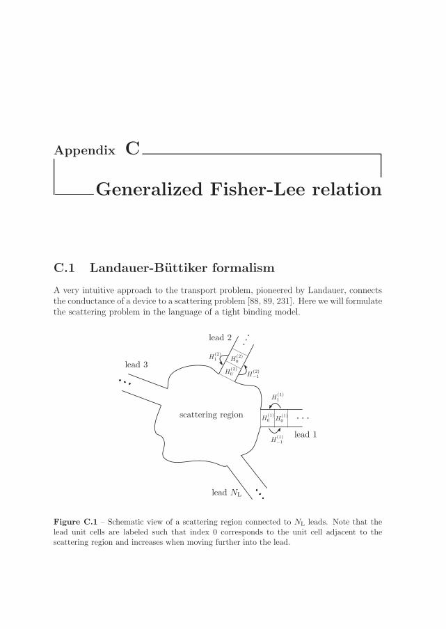
Appendix C
Generalized Fisher-Lee relation
C.1 Landauer-Buttiker formalism
A very intuitive approach to the transport problem, pioneered by Landauer, connectsthe conductance of a device to a scattering problem [88, 89, 231]. Here we will formulatethe scattering problem in the language of a tight binding model.
Figure C.1 – Schematic view of a scattering region connected to NL leads. Note that thelead unit cells are labeled such that index 0 corresponds to the unit cell adjacent to thescattering region and increases when moving further into the lead.

192 Appendix C. Generalized Fisher-Lee relation
Suppose a scattering region connected to NL leads, as depicted in Fig. C.1. As inChapter 3, we describe lead l as a semi-infinite repetition of unit cells, such that theHamiltonian of the isolated lead is given by
H(l)semi-infinite =
∞∑j=0
H(l)0 |j〉(l) 〈j|(l) +H
(l)1 |j〉(l) 〈j + 1|(l) +H
(l)−1 |j〉(l) 〈j − 1|(l) , (C.1)
where H(l)0 is the unit cell matrix and H
(l)1,−1 are the hopping matrices. Note that we
label the unit cells such that 0 denotes the unit cell adjacent to the scattering region,and the unit cell index increases as we move away from the scattering region (see
Fig. C.1). The asymptotic eigenstates ϕ(l)n for a given energy E and far away from the
scattering region are given by the eigenstates of the corresponding infinite wire. Theycan be written in the form
ϕ(l)n (j) =
1√|vn|
φ(l)n e
iknj , (C.2)
where φ(l)n is normalized to unity and obeys the equation(
E −H(l)0 −H
(l)1 eikn −H
(l)−1e
−ikn
)φ(l)
n = 0 , (C.3)
and vn is the velocity of the eigenstate, Eq. 3.19. The asymptotic eigenstates ϕ(l)n
are called the channels of lead l. As in Chapter 3, we sort the channels according totheir velocity vn. For vn > 0 we have a channel leaving the scattering region into thelead (outgoing, “<”), whereas for vn < 0 the channel enters the scattering region fromthe lead (incoming, “>”). Note that we choose the notation “>” and “<” just as inChapter 3.
A scattering-wave state Ψ(l)n for a given energy E originates from an incoming channel
ϕ(l)n,> and is scattered into outgoing channels in the different leads attached to the
scattering region. In the asymptotic region, where all evanescent waves have decayed,the scattering state can be written as
Ψ(l)n (j) =
{ϕ
(l)n,>(j) +
∑m rll,mn ϕ
(l)m,<(j) if j in lead l∑
m tl′l,mn ϕ(l′)m,<(j) if j in lead l′
. (C.4)
With the choice of wave function normalization for the channels in Eq. C.2, the trans-mission and reflection coefficients tl′l,mn and rll,mn form a unitary scattering matrix[231]. The conductance coefficients for leads l′ and l are then given by the Landauer-Buttiker formula (for further introductory reading, see Refs. [59, 60]):
Gl′l =e2
h
∑n,m
|tl′l,mn|2 . (C.5)

C.2. Generalized orthogonality relations 193
The problem of transport is thus reduced to calculating the scattering wave func-tions. However, very often it is more convenient to calculate the Green’s functioninstead of the scattering wave functions itself. We are then left with the problem toobtain the transmission coefficients from the Green’s function alone. Relations for thetransmission or reflection coefficients and the Green’s function of the system are calledFisher-Lee relations [90]. Here we will derive a generalized Fisher-Lee relation validfor any tight-binding Hamiltonian.
To this end we will closely follow Ref. [154], that derived Fisher-Lee relations forelectrons in a magnetic field. The steps there carry over to arbitrary tight-bindingHamiltonians. Note that the problem of extracting the transmission coefficients fromthe Green’s function has also been addressed in Ref. [82], utilizing the inverse matrix ofeigenvectors (U−1
< in Chapter 3). The relations derived in this chapter avoid invertingthe eigenvector matrix which can be problematic, as shown in Chapter 3. Furthermore,the expressions are more along the lines of the well-known Fisher-Lee relations forsimple systems [59, 60, 90, 231], and will provide some additional physical insight.
The derivation of the generalized Fisher-Lee relation is complicated by the fact thatthe transverse wave functions of different channels need not be orthogonal any more,as discussed in Section 3.1. If the transverse wave functions were orthogonal, thetransmission and reflection coefficients could be simply extracted from the scatteringwave function by projection. To remedy the absence of a simple orthogonality rela-tion, we derive a generalized orthogonality relation for the transverse wave functionsφn in the next section. Then, we will construct the scattering wave function fromthe Green’s function and derive expressions for the transmission and reflection coef-ficients. Finally, we emphasize the equivalence between the scattering formalism andthe non-equilibrium Green’s function formalism by showing how central results of bothformalisms are connected.
C.2 Generalized orthogonality relations
We now proceed to derive a generalized orthogonality relation for the transverse wavefunctions of propagating and decaying asymptotic eigenstates un.1 Note that theexpressions derived here are valid within a single lead l, and we will therefore drop thelead index “(l)” in this section in order to simplify notation.
By combining Eq. (3.14a) and its complex conjugate,
(E −H0)λnun =(H1λ
2n +H−1
)un and
u†n(E −H0)λ∗n =u†n
(H−1(λ
∗n)2 +H1
), (C.6)
we find that
u†n′(H1λ
2n +H−1
)unλ
∗n′ = u†n′
(H−1(λ
∗n′)
2 +H1
)unλn (C.7)
1 Remember that un denotes all eigenstates, decaying and propagating, whereas φn denotes onlypropagating eigenstates.

194 Appendix C. Generalized Fisher-Lee relation
and thusu†n′ (H1λn −H−1λ
∗n′)un (1− λnλ
∗n′) = 0 . (C.8)
This equation is trivially fulfilled if λnλ∗n′ = 1. This is the case for propagating modes
with λn = λn′ = eikn . If n = n′, the expression in the first bracket is then up to a factorthe velocity vn of the propagating mode. For n �= n′, i.e. for degenerate propagatingmodes, we have shown in Section 3.2.3, that the eigenmodes φn can be chosen such thatthey diagonalize the expression in the first bracket. In the case of decaying modes, theequation is trivially fulfilled, if λn = 1/λ∗n′, for pairs of right- (“<”) and left-decaying(“>”) modes. In all other cases, the expression in the first bracket must be zero. Insummary, we find
iu†n′ (H1λn −H−1λ∗n′) un =
⎧⎪⎨⎪⎩�vn for propagating modes with n = n′
const. for pairs of decaying modes with λn = 1/λ∗n′0 else
,
(C.9)where we have introduced a factor i to make the expression Hermitian. First, thisproves that the propagating modes φn diagonalize the velocity operator, as stated inSection 3.2.3.2 In addition, we are also provided with relations between propagatingand decaying modes.
In order to utilize these relations, we introduce the operator
K(j) =i
�(H1 |j〉 〈j + 1| −H−1 |j + 1〉 〈j|) . (C.10)
The full wave function of a decaying or propagating asymptotic state can be writtenin a compact form as ξn(j) = cunλ
jn, where c is an appropriate normalization constant
(c = 1/√|vn| for propagating modes). Note that we reserve the notation ϕn(j) for
propagating modes. Then we find the generalized orthogonality relations:
⟨ξn,<(>)
∣∣K(j)∣∣ξn′,<(>)
⟩=
{δnn′ for a propagating mode
0 else, (C.11a)
and in particular for the propagating modes:⟨ϕn,<(>)
∣∣K(j)∣∣ϕn′,<(>)
⟩= δnn′ (C.11b)⟨
ϕn,>(<)
∣∣K(j)∣∣ξn′,<(>)
⟩= 0 , (C.11c)
regardless of j.
2 Note furthermore, that if the transverse wave functions φn of the propagating modes would notdiagonalize the velocity operator, the Landauer-Buttiker formula (C.5) could also contain terms ofthe form tm1n1t
∗m2n2
with m1 �= m2 and n1 �= n2. This is an additional reason why in a numericalcalculation degenerate propagating modes must be rotated so that the velocity operator is diagonalin this basis, as described in Section 3.2.3.

C.2. Generalized orthogonality relations 195
For the purposes of implementing these operator expressions in a computer program,it is useful to rewrite them in compact matrix form. For this, note that from theexpressions for the surface Green’s function in Section 3.2.4 we obtain:
grRH−1 un,< = λn,<un,< and (C.12a)
u†n,<H1gaR = λ∗n,<u†n,< . (C.12b)
Expressions of the type grRH−1 essentially propagate a mode from one unit cell to the
other and are thus commonly called transfer matrices [97].
Using the definition Γ = i (Σr − Σa) with the lead self-energies Σr(a) = H1gr(a)R H−1,
we find
un′,<Γun,< =iun′,< (H1grRH−1 −H1g
aRH−1)un,<
=iun′,<(H1λn,< −H−1λ
∗n′,<)un,<
=
{� |vn| δnn′ for propagating modes,
0 else.(C.13)
The matrix Γ thus plays the role of a velocity or current operator within the lead.In an analogous fashion, by utilizing the expressions for ga
R, we can derive a similarexpression for modes decaying to the right and propagating in the opposite direction.
The matrix Γ is a central object that appears in many expressions of the non-equilibrium Green’s function formalism (see Section 2.5.2). In order to make connec-tions between this formalism and the scattering theory, we collect some useful identitiesfor Γ.
First, we rewrite the expression for the transfer matrix grRH−1 as
grRH−1 = U< Λ< U
−1< =
∑n
un,< λn,< u†n,< , (C.14)
where u†n,< is the n-th row of the inverse eigenvector matrix U−1< . Inserting this ex-
pression in the definition of the matrix Γ we obtain
Γ =i (H1 grRH−1 −H1 g
aRH−1)
=i(H1U< Λ< U
−1< − (U †<)−1Λ†<U
†<H−1
)=i∑
n
(H1un,< λn,< u†n,< − un,< λ
∗n,< u†n,<H−1
), (C.15)
where we utilized (grRH−1)
† = H1gaR. Now we insert unity at the appropriate places,
1 = U<U−1< =
∑m um,< u†m,< and 1 = (U †<)−1U †< =
∑m um,< u†m,<. Then we find
Γ =i∑
n
(1H1un,< λn,< u†n,< − un,< λ
∗n,< u†n,<H−1 1
)=i∑n,m
(um,< u†m,<H1un,< λn,< u†n,< − um,< λ
∗m,< u†m,<H−1un,< u†n,<
)=∑
n
φn,< �|vn,<| φ†n,< , (C.16)

196 Appendix C. Generalized Fisher-Lee relation
where we used Eq. (C.9) and |vn,<| = vn,<. Furthermore, according to Eq. (C.9)
φ†n,< = φ†n,<Γ/(�|vn,<|) (C.17)
and we obtain the final expression
Γ =∑
n
Γφn,<
1
�|vn,<|φ†n,<Γ . (C.18)
Only outgoing propagating modes φn,< contribute to the velocity/current operator Γwhich comes at no surprise, since only the propagating modes carry current. FromEq. (C.17) and the eigendecomposition expression for the transfer matrix, we immedi-ately obtain the useful relation
φ†n,<Γ grRH−1 = λn,< φ†n,<Γ (C.19)
which is the complement to Eq. (C.12a).In an analogous way, utilizing the eigenvector expression for the advanced surface
Green’s function, we can derive an expression for Γ only in terms of incoming propa-gating modes,
Γ =∑
n
Γφn,>
1
�|vn,>|φ†n,>Γ . (C.20)
Note that vn,> < 0 here. For the transfer matrices, we obtain
gaRH−1φn,> = λn,> φn,> and (C.21a)
H1grR Γφn,> = λ∗n,> Γφn,> . (C.21b)
C.3 Fisher-Lee relation
We now relate the scattering wave function Ψ(l)n to the Green’s function Gr. In order
to keep the notation simple, we assume that the Hamiltonian of the full system can bewritten in a quasi-linear form,
H =∞∑
j=−∞Hj,j |j〉 〈j|+Hj,j+1 |j〉 〈j + 1|+Hj,j−1 |j〉 〈j − 1| . (C.22)
All blocks j < 1 are supposed to correspond to lead l, |0〉 = |0〉(l) , |−1〉 = |1〉(l) , |−2〉 =
|2〉(l) , . . . , and all blocks j > L are supposed to contain all other leads, |L+ 1〉 =⊗l′ �=l |0〉
(l′) , |L+ 2〉 =⊗
l′ �=l |1〉(l′) , . . . . The Hamiltonian H can always be written
in such a form, and this form can be explicitly found by the algorithm presented inChapter 4.
We now choose a finite region of integration A containing the scattering region and asizeable part of the leads, such that the boundary ofA is in the asymptotic region of the

C.3. Fisher-Lee relation 197
Figure C.2 – The integration region A includes the scattering region and parts of the leadsup to the asymptotic region.
leads, as schematically depicted in Fig. C.2. Using Gr(E−H) = 1 and (E−H)Ψ(l)n = 0
we can write
Ψ(l)n (x) =
∑j∈A
〈x|Gr(E −H) |j〉 〈j| Ψ(l)n
⟩− 〈x|Gr |j〉 〈j| (E −H)
∣∣Ψ(l)n
⟩, for x ∈ A.
(C.23)Using the quasi-linear form of H , Eq. (C.22), and writing accordingly
∑j∈A as
∑z2
j=z1,
where z1 < 0 and z2 > L+ 1 are blocks corresponding to the boundaries of A, we findthat
Ψ(l)n (x) = 〈x|Gr |z2〉Hz2,z2+1 〈z2 + 1| Ψ(l)
n
⟩−
〈x|Gr |z2 + 1〉Hz2+1,z2 〈z2| Ψ(l)n
⟩+
〈x|Gr |z1〉Hz1,z1−1 〈z1 − 1| Ψ(l)n
⟩−
〈x|Gr |z1 − 1〉Hz1−1,z1 〈z1| Ψ(l)n
⟩. (C.24)
The sum over all lattice points within the area A has thus been reduced to a suminvolving only contributions from the surface. Hence, this can be understood as adiscrete version of Green’s theorem. Using the definition from Eq. (C.10) we finallyarrive at
Ψ(l)n (x) =
∑l′ �=l
�
i〈x|GrK(l′)(z2)
∣∣Ψ(l)n
⟩+
�
i〈x|GrK(l)(z1)
∣∣Ψ(l)n
⟩. (C.25)
The expression for the scattering wave function Ψ(l)n thus involves the operator K(l)
for which we derived generalized orthogonality relations in the previous section. Tosimplify this expression further, we consider the behavior of the Green’s function in the

198 Appendix C. Generalized Fisher-Lee relation
asymptotic region of a lead, limz→±∞ 〈x|Gr |z〉. Here, limz→±∞ should be understoodas taking z into the asymptotic region of lead l (z → −∞) and l′ �= l (z → +∞). TheGreen’s function limz→±∞ 〈x|Gr |z〉 contains only incoming waves ϕ> (for a detailed
discussion see Ref. [154]). Considering further that the scattering wave function Ψ(l)n (z)
contains incoming waves only in lead l, by virtue of the generalized orthogonalityrelations all surface terms except for the source term in lead l vanish:3
Ψ(l)n (x) = lim
z1→−∞〈x|Gr |z1〉(l)H(l)
1 〈z1 − 1|(l)∣∣Ψ(l)
n
⟩−
〈x|Gr |z1 − 1〉(l)H(l)−1 〈z1|(l)
∣∣Ψ(l)n
⟩= lim
z1→−∞
(Gr
x,z1H
(l)1
1√|vn,>|
φ(l)n,>e
−ikn,>(z1−1)−
Grx,z1+1H
(l)−1
1√|vn,>|
φ(l)n,>e
−ikn,>z1
)= lim
z1→−∞Gr
x,z1
(H1g
a,(l)R H−1 −H1g
r,(l)R H−1
) 1√|vn,>|
φ(l)n,>e
−ikn,>z1 , (C.26)
where we used Eqs. (C.21a) and (3.8). Using the definition of Γl we thus arrive finallyat
Ψ(l)n (x) = lim
z1→−∞i√|vn,>|
e−ikn,>z1 Grx,0 Γl φ
(l)n,> (C.27)
valid for any point x ∈ A. This expression is thus a viable way to calculate the fullscattering wave function in the scattering region from the Green’s function Gr.
As usual [90, 154, 231], the relation between the scattering wave function and theGreen’s function involves values of Gr in the asymptotic region, i.e. far from the scat-tering region. For numerics, this is rather inconvenient, as it implies including largeparts of the leads in the calculation, increasing computing time. It would therefore bedesirable to obtain an expression involving only the Green’s function within the firstfew layers of the lead. For this, note that from Eq. (3.8) we can write
Grz2,z1
= Grz2,z′1
(H1g
r,(l)R
)z′1−z1
(C.28)
whenever z2 is not further in lead l than z′1. In particular, we find restricting x to becontained in a block j ≥ 0
Ψ(l)n (x) = lim
z1→−∞i√|vn,>|
e−ikn,>z1 Grx,0
(H1g
r,(l)R
)−z1
Γl φ(l)n,> (C.29)
Since according to Eq. (C.21b) Γlφ(l)n,> is an eigenvector of the transfer matrix H1g
r,(l)R
with eigenvalue λ∗n,> = e−ikn,>, we finally arrive at
Ψ(l)n (x) =
i√|vn,>|
Grx,0 Γl φ
(l)n,> . (C.30)
3 When reading the formulas remember that |z1〉 = |−z1〉(l) in our notation. Therefore, additional“−”-signs appear with respect to the definition of the scattering wave-function Ψ(l)
n in Eq. (C.4)

C.4. Equivalence of scattering and NEGF formalism 199
This expression can be used directly for numerical computations.In order to calculate the transmission and reflection coefficients we do not need the
scattering wave function in the scattering region, but only in the respective leads. Inthe asymptotic region, the scattering wave function Ψ
(l)n contains only propagating
modes, as indicated by Eq. (C.4). However, as argued above, for numerical purposesit is rather inconvenient to use the asymptotic region.
Closer to the scattering region, Ψ(l)n also contains evanescent waves, decaying away in
the direction of the lead. In the previous section we have shown that φ(l′)m,> is orthogonal
to both propagating and decaying modes with respect to the current operator Γl′.Therefore, we can use this generalized orthogonality relation to project out the desiredscattering coefficients from the scattering wave function Ψ
(l)n at any point of the leads.
We first consider the case that x is in lead l′ �= l. From (φ(l′)m,>)†Γl′ Ψ
(l)n we find
tl′l,mn =i
�
1√|vm,<||vn,>|
(φ(l′)m,<)† Γl′ G
rL+1,0 Γlφ
(l)n,> . (C.31)
In the case of l′ = l, we obtain the reflection coefficients. In this case it is necessary tokeep in mind that incoming and outgoing waves need not be orthogonal with respectto Γl, and we obtain
rll,mn =1
�√|vm,<||vn,>|
(i (φ
(l)m,<)† Γl G
r0,0 Γlφ
(l)n,> − (φ
(l)m,<)† Γl φ
(l)n,>
). (C.32)
These general expressions for the transmission and reflection coefficients are very sim-ilar to the Fisher-Lee relations derived for the particular case of electrons in a two-dimensional electron gas in textbooks [59, 60]. There, in- and outgoing modes have thesame transverse wave function, φn,< = φn,> = φn, and the transverse wave functionsare eigenstates to the current operator, Γφn = �vnφn. In general, this is not the case,and one has to resort to the formulas derived here. Examples where this is the case areelectrons in a magnetic field, dealt with in Chapter 3 of this work, and zigzag graphenenanoribbons, Chapters 6 and 7.
C.4 Equivalence of scattering and non-equilibrium
Green’s function formalism
The generalized Fisher-Lee relation allows to relate central results from the non-equilibrium Green’s function (NEGF) formalism with concepts from the Landauer-Buttiker formalism based on a scattering problem.
In the NEGF formalism, Eq. (2.119), we obtained the conductance between two leadsl and l′ in linear response as
Gll′ =e2
hTr (ΓlG
r Γl′ Ga) . (C.33)

200 Appendix C. Generalized Fisher-Lee relation
Expressing the current operators Γ(l),(l′) in terms of in- and outgoing modes, Eqs. (C.18)and (C.20) we find
Gll′ =e2
hTr (ΓlG
r Γl′ Ga)
=e2
hTr(∑
n
Γlφ(l)n,<
1
�|vn,<|(φ
(l)n,<)†Γl G
r∑m
Γl′φ(l′)m,>
1
�|vm,>|(φ
(l′)m,>)†Γl′ G
a)
=e2
h
∑m,n
1
�2 |vn,<||vm,>|((φ
(l)n,<)†ΓlG
rΓl′φ(l′)m,>
)((φ
(l′)m,>)†Γl′G
aΓlφ(l)n,<
)=e2
h
∑m,n
|tll′,nm|2 , (C.34)
where we made use of the Fisher-Lee relation (C.31). Thus, the NEGF expression forthe conductance in linear response is equivalent to the Landauer-Buttiker formula.
Another important relation from the NEGF formalism is the expression for the lesserGreen’s function from the Keldysh equation, Eq. (2.95),
G< = GrΣ<Ga . (C.35)
In the case of non-interacting electrons, or for Coulomb interaction in Hartree-Fockapproximation, Σ< only contains contributions from the leads and can be written as
Σ<(E) =∑
l
iΓl f(E, μl) , (C.36)
where μl is the electrochemical potential in lead l. The contribution of a single lead lto G< is given by
G<,(l)(x,x′) = Gr iΓlf(E, μl)Ga
= f(E, μl)∑
n
i Gr Γlφ(l)n,>
1
�|vn,>|(φ
(l)n,>)†Γl G
a
∝ f(E, μl)∑
n
iΨ(l)n (x)(Ψ(l)
n (x′))∗1
�|vn,>|. (C.37)
Note that we neglected possible constant terms in the last line, in order to avoiddiscussing the appropriate normalization of the scattering wave functions. The term1/|vn,>| is up to a constant the one-dimensional density of states of the incoming
channel n in lead l [89], and we denote this density of states as D1d,(l)n (E). The full
lesser Green’s function thus reads
G<(x,x′, E) ∝∑
l
f(E, μl)∑
n
iΨ(l)n (x)(Ψ(l)
n (x′))∗D1d,(l)n (E) . (C.38)
Hence, the lesser Green’s function, and thus in particular the electron density for a givenenergy E, is composed of all scattering states, weighted with the respective density ofstates of the incoming channel and the Fermi function of the respective lead.

Appendix D
Details of the derivationof the lead Green’s function
D.1 λ(E + iη) for propagating modes
In the derivation of the general expression for the surface Green’s function of a lead itis necessary to determine which poles contribute to the contour integral in Eq. (3.12).That is, we need to determine whether the eigenvalues λn of the quadratic eigenvalueequation (
(E + iη −H0)λn −H1λ2n −H−1
)un = 0 (D.1)
are located inside or outside the unit circle. For any eigenvalue with |λn| �= 1 thiscan be done without considering the infinitesimal shift iη. However, in the case of apropagating mode un = φn, we find that the eigenvalue λn = eik and thus lies directlyon the unit circle, if we neglect the infinitesimal shift iη. Therefore, it is vital to includeiη in the calculation for this case.
Numerically, this could be done by explicitly including some small but final imaginarypart of the energy E in the calculation [102]. However, this just introduces a parameterinto the numerical calculation that might need manual adjustment in order to achieveconvergence. Therefore we will show in the following, how we can determine λn(E+ iη)for the solution including the infinitesimal shift iη from the properties of the solutionλn(E), φn(E) of the quadratic eigenvalue problem without the infinitesimal iη:(
(E −H0)λn(E)−H1λn(E)2 −H−1
)φn(E) = 0 . (D.2)
In the course of this derivation we will also gain some insight into the arguments usedin the derivation of the lead Green’s function in Refs. [59, 82, 86] and justify thesearguments mathematically.

202 Appendix D. Details of the derivation of the lead Green’s function
In order to determine the solution including the infinitesimal shift iη we use theTaylor expansion
λn(E + iη) = λn(E) +dλn
dE
∣∣∣∣E
iη +O(η2) . (D.3)
Note that a similar approaches have been used in Refs. [94, 100, 103].In order to calculate dλn
dEwe take the derivative of Eq. (D.2) with respect to the
energy: (λn(E) + (E −H0)
dλn
dE−H1 2λ(E)
dλn
dE
)φ(E)+
((E −H0)λn(E)−H1λn(E)2 −H−1
) dφn
dE= 0 . (D.4)
Using the fact that, as shown in Section 3.2.2, φ†n is also a right eigenvector of thequadratic eigenvalue problem Eq. (D.2), we can get rid of the second term of Eq. (D.4)and find
φ†n(E)
(λn(E) + (E −H0)
dλn
dE−H1 2λ(E)
dλn
dE
)φ(E) = 0 . (D.5)
Further exploiting the fact that the φn are normalized, φ†nφn = 1, we arrive at theexpression
dλn
dE
∣∣∣∣E
=λn(E)
2φ†nH1φn λn(E)− φ†n (E −H0) φn
. (D.6)
To determine whether λn(E + iη) lies inside or outside the unit circle, we need tocalculate |λn(E + iη)|. Using the Taylor expansion (D.3) we find
|λn(E + iη)| =|λn(E) +dλn
dEiη +O(η2)|
=
(λn(E) +
dλn
dEiη +O(η2)
)(λ∗n(E)−
(dλn
dE
)∗iη +O(η2)
)=|λn(E)|2 + iη
(λ∗n(E)
dλn
dE− λn(E)
(dλn
dE
)∗)+O(η2)
=1− 2 η Im
(λ∗n(E)
dλn
dE
)+O(η2) . (D.7)
Using Eq. (D.6) we find
λ∗n(E)dλn
dE=
λ∗n(E)λn(E)
2φ†nH1φn λn(E)− φ†n (E −H0)φn
=1
2φ†nH1φn λn(E)︸ ︷︷ ︸�
−φ†n (E −H0)φn︸ ︷︷ ︸�
. (D.8)

D.2. Derivation of Eq. (3.27) 203
Since for real energy E—and only for real energies we can have propagating modes—the matrix E −H0 is hermitian, term � in the equation above is real, and only term� contributes to the imaginary part. Furthermore, note that the imaginary part ofterm � is related to the velocity of the propagating mode according to Eq. (3.19).Combining this information we finally arrive at
Im
(λ∗n(E)
dλn
dE
)= −Im
(2φ†nH1φn λn(E)
)|. . .|︸︷︷︸>0
=� vn(E)
|. . .| , (D.9)
and thus|λn(E + iη)| = 1− 2�
η
|. . .|︸ ︷︷ ︸>0
vn(E) +O(η2) . (D.10)
In summary we find that for a propagating mode φn(E) λn(E + iη) lies
• inside the unit circle, if vn(E) > 0, i.e. for right-moving modes,
• inside the unit circle, if vn(E) < 0, i.e. for left-moving modes.
This criterion only fails for vn = 0, i.e. directly at a band edge. However, vn = 0 alsoimplies a diverging density of states and thus impedes a numerical calculation of theGreen’s function anyways. In such a situation it is advisable to move away a little bitfrom the band edge.
Refs. [59, 82, 86] directly invoke the concept of left- and right-going modes in orderto fulfill the boundary conditions of retarded and advanced Green’s function, i.e. in-and outgoing waves. The calculations of this section justify these assumptions mathe-matically.
D.2 Derivation of Eq. (3.27)
We shall now show how to derive Eq. (3.27). In Eq. (3.26) we have
Grj,j′ =
1
2πi
∮dz U< zj−j′ (h(z))−1 for j′ ≤ j, (D.11)
where we defined h(z) = H(E + iη, z)U<.In order to solve the contour integral of Eq. (D.11) we need to consider each com-
ponent of the inverse matrix h(z)−1 separately. The components of the inverse matrixare given by (
h(z)−1)
ij=
1
det(h(z))adj(h(z)) , (D.12)
where adj(h(z)) is the adjugate of the matrix h(z). (h(z)−1)ij is thus a rational func-tion and we need to determine the zeroes of denominator and numerator and theirmultiplicities in order to solve the contour integral.

204 Appendix D. Details of the derivation of the lead Green’s function
First, we consider the denominator. We have det(h(z)) = det(H(E+iη, z)) det(U<).det(U<) is simply a constant. Therefore we find
det(h(z)) ∝∏n
(z − λn,<)∏n
(z − λn,>) , (D.13)
as det(H(E+ iη, z)) = 0 for z = λn,</>. Note that for a rank-deficient hopping matrixH1, some of the eigenvalues are infinite. The expression above contains contains finiteeigenvalues, and det(h(z)) is a polynomial of degree N + rank(H1).
Next, we examine the numerator further. The adjugate of the matrix h(z) is given byadj(h(z))ij = (−1)i+jMji where Mji is given by the determinant of the matrix resultingfrom deleting row j and column i from h(z). Let SN\i denote the set of permutationsof the numbers {1, . . . , i− 1, i+ 1, . . . , N}. Using the Leibniz formula for determinantswe can write
adj(h(z))ij = (−1)i+j∑
σ∈SN\i
sgn(σ)
N∏n=1n �=j
h(z)nσ(n) . (D.14)
The matrix h(z) has columns that have definite zeroes at λn,<: We can write
h(z) = H(E + iη, z)U< =(H(E + iη, z)u1,<
∣∣∣ . . . ∣∣∣H(E + iη, z)uN,<
). (D.15)
Since H(E+iη, z = λn,<)un,< = 0, the entries of the matrix hij(z) = (H(E+iη, z)uj,<)i
have a zero of at least multiplicity one at λj,<. Thus we find that
adj(h(z))ij = C(z)N∏
n=1n �=i
(z − λn,<) , (D.16)
where C(z) is some polynomial.Combining the expressions for the numerator and the denominator we find(
h(z)−1)
ij=
1
z − λi,<D(z)
∏n
1
z − λn,>, (D.17)
where D(z) is some polynomial. Only the eigenvalues inside the unit circle, λn,<,contribute to the contour integral (D.11). Thus we can ignore the poles at λn,> andabsorb them in the definition of D(z). In order to solve the integral we need todistinguish two cases:
• D(λi,<) �= 0. In this case, (h(z)−1)ij has a simple pole at λi,< and we find
1
2πi
∮dz zj−j′ (h(z)−1
)ij
=1
2πi
∮dzzj−j′D(z)
z − λi,<
=(λi,<)j−j′D(λi,<)
= (λi,<)j−j′ 1
2πi
∮dz(h(z)−1
)ij. (D.18)

D.3. Summary of the numerical algorithms 205
Note that this equation also holds for λi,< = 0, when zj−j′ (h(z)−1)ij is an analyticfunction within the unit circle.
• D(λi,<) = 0. In this case, (h(z)−1)ij is an analytic function within the unit circleand
1
2πi
∮dz zj−j′ (h(z)−1
)ij
=1
2πi
∮dz(h(z)−1
)ij
= 0 . (D.19)
Hence, we can still write
1
2πi
∮dz zj−j′ (h(z)−1
)ij
= (λi,<)j−j′ 1
2πi
∮dz(h(z)−1
)ij. (D.20)
Finally, from Eqs. (D.18) and (D.20) we find
Grj,j′ =
1
2πi
∮dz U< zj−j′ (h(z))−1 =
1
2πi
∮dz U< Λj−j′
< (h(z))−1 for j′ ≤ j, (D.21)
where Λ< is a diagonal matrix with entries (Λ<)nn = λn,<. This concludes the proof ofEq. (3.27).
It should be noted that during the derivation it was assumed that j′ ≤ j. If j′ >j, zj−j′ = 1/zj′−j introduces additional poles in the contour integral. However, bysubstituting y = 1/z we an can perform an analogous calculation, but in this case onlythe eigenvalues outside the unit circle contribute.
D.3 Summary of the numerical algorithms
D.3.1 Eigendecomposition based algorithms
The results from Section 3.2 allow for the computation of the surface Green’s functionfor arbitrary tight-binding models. Here, we summarize the numerical algorithms,distinguishing the two cases of invertible and non-invertible hopping matrix H1.
Algorithm D.1. Invertible hopping matrix H1
A From H0, H1, and H−1 build up the matrix
A =
(0 1
− (H1)−1 H−1 (H1)
−1 (E −H0)
). (D.22)
B Solve the eigenproblem
A
(un
λnun
)= λn
(un
λnun
), (D.23)
and extract the 2N eigenvectors un and eigenvalues λn of the quadratic eigen-problem.

206 Appendix D. Details of the derivation of the lead Green’s function
C Identify degenerate eigenvalues of the form λ = eik and rotate the correspondingeigenvectors by diagonalizing the velocity operator.
D Build up the matrices U< and Λ< from the right-going eigenstates.
E Calculate the surface Green’s function as
grR = U< Λ< U
−1< (H−1)
−1 . (D.24)
Implementation: The eigenvalue problem can be solved numerically by the LAPACKroutine ZGEEV. LAPACK also provides standard routines for matrix multiplication andinversion [107].
Algorithm D.2. Singular hopping matrix H1
A From H0, H1, and H−1 build up the matrices
A =
(0 1
−H−1 E −H0
)and B =
(1 00 H1
)(D.25)
B Solve the generalized eigenproblem
A
(un
λnun
)= λnB
(un
λnun
), (D.26)
and extract the 2N eigenvectors un and eigenvalues λn of the quadratic eigen-problem.
C Identify degenerate eigenvalues of the form λ = eik and rotate the correspondingeigenvectors by diagonalizing the velocity operator.
D Build up the matrices U< and Λ< from the right-going eigenstates.
E Calculate the surface Green’s function as
grR =
(E −H0 −H1U< Λ< U
−1<
)−1(D.27)
Implementation: The generalized eigenproblem can be solved numerically by theLAPACK routine ZGGEV [107]. Note that the numerical algorithms in LAPACK solvethe generalized eigenvalue problem in the form
βAu = αBu , (D.28)
such that λ = α/β. In this way, even λ = ∞ is well-defined as β = 0.
D.3.2 Schur decomposition based algorithms
The results from Section 3.3 allow for a more stable calculation of the lead Green’sfunction in terms of the (generalized) Schur decomposition. We now summarize thecomputational steps, distinguishing again the cases of invertible and singular hoppingmatrices H1.

D.3. Summary of the numerical algorithms 207
The algorithms are valid as long as λn,< and λn,> do not contain the same eigen-values. Otherwise, i.e. in situations as depicted in Fig. 3.3(c), the energy E must beshifted slightly before starting the calculation.
Algorithm D.3. Invertible hopping matrix H1
A From H0, H1, and H−1 build up the matrix
A =
(0 1
− (H1)−1 H−1 (H1)
−1 (E −H0)
). (D.29)
B Calculate the Schur decomposition Q†AQ = T and extract the eigenvalues λn.
C Calculate the eigenvectors φn of A for all propagating modes, i.e. |λn| = 1
D For those propagating modes, identify degenerate eigenvalues of the form λn = λn′
and rotate the corresponding eigenvectors by diagonalizing the velocity operator.
E Classify the eigenvalues into left- and right-going using the calculated eigenvectorsφn for propagating modes.
F Reorder the Schur decomposition such that the eigenvalues λn,< appear on theleading diagonal positions of the triangular matrix T , and update Q accordingly.
G Calculate the surface Green’s function as
grR = Q21Q
−111 (H−1)
−1 . (D.30)
Implementation: This algorithm can be fully implemented with routines from LA-PACK [107]. The Schur decomposition is calculated using ZGEHRD, ZUNGHR and ZHSEQR.The eigenvectors for propagating modes are computed using inverse iteration [112] withZHSEIN. Finally, the routine ZTRSEN is applied to reorder the Schur decomposition.
Algorithm D.4. Singular hopping matrix H1
A From H0, H1, and H−1 build up the matrices
A =
(0 1
−H−1 E −H0
)and B =
(1 00 H1
)(D.31)
B Calculate the generalized Schur decomposition Q†AZ = T and Q†BZ = S, andextract the eigenvalues λn = tnn/snn. Note that only the transformation Z needsto be calculated explicitly.
C Calculate the eigenvectors φn for all propagating modes, i.e. |λn| = 1
D For those propagating modes, identify degenerate eigenvalues of the form λn = λn′
and rotate the corresponding eigenvectors by diagonalizing the velocity operator.
E Classify the eigenvalues into left- and right-going using the velocities calculatedfrom the eigenvectors φn for propagating modes.

208 Appendix D. Details of the derivation of the lead Green’s function
F Reorder the generalized Schur decomposition such that the eigenvalues λn,< ap-pear on the leading diagonal positions of the triangular matrices T and S, andupdate Z accordingly.
G Calculate the surface Green’s function as
grR =
(E −H0 −H1Z21Z
−111
)−1(D.32)
Implementation: Again, LAPACK provides all routines necessary for the compu-tation. The generalized Schur decomposition is computed using ZGGES and from thatthe eigenvectors for propagating modes using ZTGEVC. The routine ZTGSEN reorders thegeneralized Schur decomposition.

Appendix E
The Fiduccia-Mattheyses algorithm
E.1 Graphs and hypergraphs
The Fiduccia-Mattheyses algorithm was originally developed for hypergraph partition-ing [132]. A hypergraph H is an ordered pair H = (V,N ), where V is a set of vertices,and N a set of nets (also called hyperedges) between them. A net ni ∈ N is a setof vertices, i.e. ni ⊂ V. An undirected graph is a special realization of a hypergraph,where every net contains exactly two vertices. Thus, any algorithm for hypergraphpartitioning can also be applied to an undirected graph.
During the FM bisection, we have to consider the graph structure arising from theHamiltonian matrix in order to minimize the number of cut edges (min-cut), whereasfor minimizing the number of surface vertices, i.e. the number of cut nets (min-net-cut), the hypergraph structure arising from all nets net(v) as defined in Eq. (4.11),N = {net(v) | v ∈ V}, is essential. For min-net-cut-min-cut optimization, we have toconsider both structures simultaneously. A schematic representation of a graph andthe corresponding hypergraph structure is shown in Fig. E.1.
Figure E.1 – Schematic representation of (a) a simple graph and (b) the correspondinghypergraph structure imposed through all nets, N = {net(v) | v ∈ V}.

210 Appendix E. The Fiduccia-Mattheyses algorithm
E.2 Fiduccia-Mattheyses bisection
The FM algorithm is based on the concept of gain. The gain of a vertex in an existingbisection is defined as the change in weight, i.e. the number of cut edges or nets, thatoccurs when this vertex is moved to the other part. This gain can also be negative,if such a move increases the number of cut edges or nets. The basic idea of theFM algorithm is to swap vertices with the highest gain between parts, while obeyingsome balance criterion. The fact that the highest gain can be negative, helps the FMalgorithm to escape local minima. After moving, the respective vertex is locked inorder to avoid an infinite loop, where a single vertex might be swapped back and forthrepeatedly. The FM pass ends, when all (free) vertices have been moved, and the bestbisection encountered during the pass is returned as result. Further passes can thensuccessively improve on this bisection.

Appendix F
The method of finite differences
F.1 Basic ideas
The fundamental concept behind the method of finite differences go back to Newtonand his contemporaries: Replace the derivative of a function by a difference quotient.With this replacement, a differential equation is reduced to a set of algebraic equations,that can easily be solved on a computer. In fact, the method of finite differences wasalready used for a numerical solution of the Schrodinger equation before the advent ofelectronic computers [77].
The approximations needed in the method of finite differences are most convenientlyremembered from the Taylor expansion of a function f :
f(x+ h) = f(x) + f ′(x) h+O(h2)
(F.1)
and
f(x− h) = f(x)− f ′(x) h+O(h2). (F.2)
Subtracting Eq. (F.2) from Eq. (F.1), we obtain the symmetric approximation for thederivative of a function,
f ′(x) =f(x+ h)− f(x− h)
2a+O
(h2), (F.3)
whereas adding Eqs. (F.1) and (F.2), we obtain an approximation for the functionitself:
f(x) =1
2(f(x+ h) + f(x− h)) +O
(h2). (F.4)
At first glance, Eq. (F.4) may not seem very useful. However, it can be used con-veniently to bring the finite difference expressions into a symmetric form, yielding a

212 Appendix F. The method of finite differences
Figure F.1 – Grids used for the method of finite differences: (a) square grid with latticeconstant a0 in two dimensions. (b) cubic grid with lattice constant a0 in three dimensions.
Hermitian Hamiltonian. Note that Eqs. (F.3) and (F.4) are valid up to second or-der in h. It is possible to use higher-order approximation formulas (see, for example,Ref. [232]), but we will restrict ourselves to the lowest order in this work.
In the method of finite differences, functions are not evaluated in the continuum, butonly on a discrete set of grid points. The simplest grids in two and three dimensions arethe uniform square and cubic grids with lattice constant a0, shown in Fig. F.1. UsingEqs. (F.3) and (F.4) with h = a0 and h = a0/2 when appropriate, it is possible toreduce a differential equation to a closed set of linear equations involving only functionvalues on the grid points.
F.2 Example
In order to put the general ideas of the previous section into practice and to illustratethe typical steps in deriving a finite differences approximation to a Hamiltonian, weconsider one example in great detail. Another detailed example can be found in theappendix of Ref. [155].
Consider the Hamiltonian H acting on the wave function ϕ(x)
Hϕ(x) =1
2
((−i�∂x + eA(x))α(x)ϕ(x) + α(x) (−i�∂x + eA(x))ϕ(x)
)=
1
2
(−i�
(∂x(α(x)ϕ(x)) + α(x) (∂xϕ(x))
)+ 2e
(A(x)α(x)ϕ(x)
)). (F.5)
Such terms arises from the Bychkov-Rashba Hamiltonian with a position-dependentBychkov-Rashba parameter α(x) in a magnetic field with vector potential A(x) (seeEq. (F.16)). Using (F.3), the first bracket in the last line of Eq. (F.5) can be rewrittenas
∂x(α(x)ϕ(x)) + α(x) (∂xϕ(x)) ≈1
2a0
((α(x) + α(x+ a0))ϕ(x+ a0)− (α(x) + α(x− a0))ϕ(x− a0)
)(F.6)
The second bracket in the last line of Eq. (F.5) is conveniently recast into a more

F.3. Finite differences form of the Hamiltonian 213
symmetric form as
A(x)α(x)ϕ(x) =1
4
((A(x)α(x))ϕ(x) + A(x)(α(x)ϕ(x))
+ α(x)(A(x)ϕ(x)) + (A(x)α(x)ϕ(x)))
≈ 1
8
((α(x) + α(x+ a0)) (A(x) + A(x+ a0))ϕ(x+ a0)
+ (α(x) + α(x− a0)) (A(x) + A(x− a0))ϕ(x− a0)), (F.7)
where we used Eq. (F.4) on every one of the expressions in the inner brackets of thefirst line. Combining all terms, we finally arrive at
Hϕ(x) ≈ − i�
2a0
1
2(α(x) + α(x+ a0))ϕ(x+ a0)
(1 +
iea0
�
1
2(A(x) + A(x+ a0))
)+
i�
2a0
1
2(α(x) + α(x− a0))ϕ(x− a0)
(1− iea0
�
1
2(A(x) + A(x+ a0))
).
(F.8)
Introducing the notation |x〉 for a state at grid point x, we can write Hϕ(x) = 〈x|H |ϕ〉and then read off the operator H from Eq. (F.8):
H ≈∑
x
− i�
2a0
1
2(α(x) + α(x+ a0)) e
iea0�
12(A(x)+A(x+a0)) |x〉 〈x+ a0|+ h.c. , (F.9)
where h.c. denotes the Hermitian conjugate of the previous expression. In order toarrive at this expression, we have made use of the fact that all approximations madeso far are valid up to second order in a0, and hence
1 +iea0
�
1
2(A(x) + A(x+ a0)) ≈ e
iea0�
12(A(x)+A(x+a0)) . (F.10)
The operator form of H in Eq. (F.9) has the form of a tight-binding operator. Inthis particular example, the Hamiltonian consists of a “hopping term” from point x tox+ a0, i.e. hopping between neighboring grid points. The magnetic field enters in theHamiltonian in the form of a Peierls phase [233]
eiea0
�
12(A(x)+A(x+a0)) ≈ e
ie�
R x+a0x
ds·A(x) . (F.11)
Because of this formal equivalence, the discretization procedure in the method of finitedifferences is said to yield a tight-binding representation of the Hamiltonian H .
F.3 Finite differences form of the Hamiltonian
After explicitly deriving the tight-binding representation of a particular example, wewill now state the finite differences forms of several terms to the Hamiltonian encoun-tered in this work. The expressions stated here are mostly valid in two (x = (x, y))

214 Appendix F. The method of finite differences
and in three dimensions (x = x, y, z). For brevity, we will not explicitly write out coor-dinates that remain unchanged, i.e. do not contribute a hopping term. In addition, wewill not explicitly include a magnetic field. In order to include the effect of a magneticfield, every hopping term must be multiplied by the Peierls phase (as in the previousexample, see Eq. (F.11)). As a general guideline, if a Hamiltonian contains parametersthat exhibit a discontinuity, the grid should be chosen such that the discontinuity lieshalfway between two grid points [234].
Kinetic energy: The kinetic energy Hamiltonian with a position-dependent massm(x) [235] reads
Hkin =1
2p
1
m(x)p , (F.12)
where p = −i�∇. The tight-binding representation is given as
Hkin =∑x
(1
m(x− a0
2)
+1
m(x+ a0
2)
)|x〉 〈x|
−(
1
m(x+ a0
2)|x〉 〈x+ a| + h.c.
)+ analogous terms for the y and z-direction . (F.13)
In the numerical calculation it is sometimes advantageous to substitute m(x + a0
2) →
12(m(x) +m(x+ a0)) [234].
Potential energy: A potential enters the Hamiltonian as
Hpot = V (x) (F.14)
and in tight-binding representation simply reads
Hpot =∑x
V (x) |x〉 〈x| . (F.15)
Bychkov-Rashba spin-orbit coupling: The Bychkov-Rashba spin-orbit couplingHamiltonian [21, 22] with a position-dependent Bychkov-Rashba parameter α(x) reads
HBR =1
2�α(x) (σxpy − σypx) +
1
2�(σxpy − σypx)α(x) , (F.16)
where σ is the vector of Pauli matrices. Note that the Hamiltonian is symmetrizedsuch that it is Hermitian (see Ref. [153, Chap. 3]). The tight-binding representation isthen given as
HBR =∑x
−i2a0
σx 1
2(α(y) + α(y + a0)) |y〉 〈y + a|+ h.c.
+i
2a0σy 1
2(α(x) + α(x+ a0)) |x〉 〈x+ a|+ h.c. . (F.17)

F.4. Bloch’s theorem and periodic boundary conditions 215
Dresselhaus spin-orbit coupling: The Dresselhaus spin-orbit coupling Hamilto-nian [236] with a position-dependent Dresselhaus parameter γ(z) reads
HD =1
�(σxpx − σypy)
∂
∂z
(γ(z)
∂
∂z
)(F.18)
and in tight-binding representation
HD =−i2a3
0
σx∑x
γ(z +
a0
2
)|x, y, z〉 〈x+ a0, y, z + a0|
+ γ(z − a0
2
)|x, y, z〉 〈x+ a0, y, z − a0|
−(γ(z − a0
2
)+ γ(z +
a0
2
))|x, y, z〉 〈x+ a0, y, z|
i
2a30
σy∑x
γ(z +
a0
2
)|x, y, z〉 〈x, y + a0, z + a0|
+ γ(z − a0
2
)|x, y, z〉 〈x, y + a0, z − a0|
−(γ(z − a0
2
)+ γ(z +
a0
2
))|x, y, z〉 〈x, y + a0, z|
+Hermitian conjugate of the whole expression. (F.19)
Note that in contrast to the previous expressions the tight-binding representation ofthe Dresselhaus parameter includes next-nearest neighbor hopping terms. Again, itmay be useful to substitute γ(z + a0
2)→ 1
2(γ(z) + γ(z + a0)).
F.4 Bloch’s theorem and periodic boundary condi-
tions
If a tight-binding Hamiltonian has a translational symmetry in some direction, Bloch’stheorem can be used to reduce the size of the problem.
As example, consider a square grid, which is translationally invariant under a shiftof Nya0, i.e. is composed of periodically repeated supercells with Ny lattice points inthe y-direction (see Fig. F.2(a)). From Bloch’s theorem, we can write
ϕ(x, y +Nya0) = eikyNya0ϕ(x, y) , (F.20)
where ky ∈ [− πNya0
, πNya0
]. In particular, this also holds for grid points at the boundary
of the supercell. Let y1 and y2 denote the lower and upper row of grid points in thesupercell. Then
ϕ(x, y2 + a0) = eikyNya0ϕ(x, y1) . (F.21)
Within the tight-binding Hamiltonian we can then replace hopping terms at the bound-ary as
|y2〉 〈y2 + a0| → eikyNya0 |y2〉 〈y1| (F.22)

216 Appendix F. The method of finite differences
Figure F.2 – (a) A square grid consisting of a periodic repetition of supercells in the y-direction. (b) Effective structure after the application of Bloch’s theorem.
and|y1〉 〈y1 − a0| → e−ikyNya0 |y1〉 〈y2| . (F.23)
Hence, the system size has an effective width of Ny grid points in the y-direction,however with additional hopping terms from the top to the bottom of the supercelland vice versa, with a phase given by the Bloch wave vector ky.
Note that if we set ky = 0, we obtain the conventional “periodic boundary condi-tions”. Neglecting all other Bloch vectors ky is a good approximation, if Nya0 is large,i.e. ky small. If this is not the case, the desired calculation must be performed for a setof ky-values.

Appendix G
Tight-binding model for graphene
G.1 Lattice structure
Graphene is a two-dimensional realization of carbon, where the carbon atoms are ar-ranged in a honeycomb network. The honeycomb network itself is not a Bravais lattice,but can be described as a triangular (or hexagonal) lattice with a basis of two atoms[93].
The triangular lattice is generated by the primitive basis vectors
a1 =
(a0
)and a2 =
( 12a√
32a
), (G.1)
as shown in Fig. G.1(a). The primitive unit cell spanned by these vectors is a rhombuswith side length a. In the case of the honeycomb network, there are two basis atomsper unit cell at the positions
dA =
(00
)and dB =
(0
1√3a
). (G.2)
We will denote these basis atoms as atom A and B respectively. It should be emphasizedthat, although we label these basis atoms differently, within the infinitely extendedhoneycomb network, they are equivalent. The basis atoms form two triangular lattices(sublattice A and B, respectively), that are shifted with respect to each other to obtainthe honeycomb network. In this network, each atom has three nearest neighbors of theopposite kind. The distance between neighboring carbon atoms is given as aCC = a/
√3.
In the case of a triangular lattice, the reciprocal is again triangular, rotated by 90◦
with respect to the original lattice, as shown in Fig. G.1(b). The reciprocal lattice isspanned by the primitive basis vectors [93]
b1 =
( 2πa2π√3a
)and b2 =
(04π√3a
). (G.3)

218 Appendix G. Tight-binding model for graphene
Figure G.1 – (a) Honeycomb network of carbon atoms. The underlying triangular Bravaislattice is spanned by the primitive basis vectors a1 and a2, shown in blue. The primitive unitcell is a rhombus, as depicted by the red dashed lines. The two basis atoms are shown asblack (sublattice A) and white (sublattice B) dots, respectively. (b) Geometrical details of ahexagon from the honeycomb network, formed by carbon atoms (c) The reciprocal lattice isspanned by the reciprocal basis vectors b1 and b2, shown in blue. The first Brillouin zone hasa hexagonal shape. (d) Geometrical details of the first Brillouin zone, showing the reciprocallattice vectors connecting the three equivalent K ′-corners.
The first Brillouin zone is constructed as the Wigner-Seitz cell of the reciprocal lattice[93] and has the shape of a hexagon. However, a wave vector in a Bravais lattice isonly defined up to some reciprocal lattice vector. Thus, only two of the six corners inthe Brillouin zone are non-equivalent, as always three corners can be connected witha reciprocal lattice vector. These two inequivalent corners are called K-points and arelabeled K and K ′ respectively. For simplicity, we choose the wave vectors
K =
(4π3a
0
)and K′ =
(−4π
3a
0
)(G.4)
to represent the two K-points.
It should be emphasized that the hexagonal shape of the Brillouin zone, and thusthe existence of two K-points, is solely due to the underlying triangular Bravais latticestructure of the honeycomb network. The reciprocal lattice only depends on the Bravaislattice structure, not on the basis atoms per unit cell. In particular, the hexagonalshape of the Brillouin zone is not related to the hexagons formed by carbon atoms inthe honeycomb network.

G.2. Electronic structure 219
G.2 Electronic structure
G.2.1 Tight-binding model
We consider the dynamics of electrons in the graphene lattice assuming that the effectof interactions can be incorporated by a mean field (non-interacting electrons; for ajustification see e.g. [237, Chap. 5]). In this case, the single-particle Hamiltonian of thesystem is given as
H = − �2
2m∇2 + Veff(x) + Vext(x) , (G.5)
where Veff(x) incorporates both the potential arising from the ions within the graphenelattice and the effect of interaction in an approximate way, and Vext is some externalpotential. Note that in the case of an infinite graphene sheet, Veff(x) has the full sym-metry of the graphene lattice. We now intend to develop a tight-binding formulationfor this problem, as was done first by Wallace in 1947 [238].
Carbon is the sixth element in the periodic table, and has 4 valence electrons in2s22p2 configuration. In graphene (and graphite, from which graphene originates),three of the valence electrons hybridize in a 2sp2 configuration. These electrons formbonds with the neighboring carbon atoms, leading to the honeycomb arrangementof carbon atoms. The fourth electron resides in a 2pz-orbital perpendicular to thegraphene plane. The electrons that form the bonds to the neighboring carbon atomswill not contribute to transport due to their bound nature, and we can therefore treatgraphene as having one electron per carbon atom in the 2pz state.
Following the arguments above, we describe graphene in tight-binding approximationwith a single orbital per basis atom. The orbital at an atom situated at Ri + dα isgiven as
χi,α,s(x) = χ2pz,s(x−Ri − dα) (G.6)
where i denotes the (Bravais) lattice vector Ri = na1+ma2 (n,m ∈ Z), α the sublattice(α = A,B) and s the spin. χ2pz,s(x − Ri − da) is the wave function of a 2pz-orbitalcentered at atom α in the unit cell at the lattice point Ri, with spin s. The quantummechanical state corresponding to the wave function χi,α,s(x) will be denoted as |i, α, s〉.As discussed in Section 2.5.1, we assume that the states |i, α, s〉 form an orthonormalset, thus neglecting overlap between wave functions located at different atoms. Withinthis basis, the tight-binding Hamiltonian reads
H =∑
i,α,j,β,s,s′〈i, α, s|H |j, β, s′〉 |i, α, s〉 〈j, β, s′| . (G.7)
In the remainder of this chapter we will only consider systems where spin is a goodquantum number, and suppress the spin index s in the notation. In this case, spinonly enters in a twofold occupation of energy levels. When we consider spin-dependenttransport properties of graphene nanoribbons in Chapter 7, we will explicitly discusshow spin-dependent terms enter the Hamiltonian.

220 Appendix G. Tight-binding model for graphene
Figure G.2 – The nearest neighbors of an A atom are three B atoms (connections shown assolid black lines), the next-nearest neighbors are six A atoms (connections shown as dashedblack lines).
In the spin-less case, the Hamiltonian reads
H =∑
i,α,j,β
tiαjβ |i, α〉 〈j, β| , (G.8)
where tiαjβ = 〈iα|H |jβ〉. The solution has the form
|ϕ〉 =∑i,α
ϕα(i) |i, α〉 , (G.9)
where ϕα(i) is the probability amplitude of occupying the orbital state |i, α〉. In real-space, the wave function reads
ϕ(x) =∑i,α
ϕα(i)χ2pz(x−Ri − dα) . (G.10)
Thus, due to the localized nature of the atomic orbitals, |ϕα(i)|2 can be roughly inter-preted as the probability of being close to the atomic site Ri + dα.
The fact that the atomic orbitals are localized is also the reason why only a few of thematrix elements tiαjβ are nonzero. Here, we will only consider matrix elements involvingorbitals at the same site, and orbitals that are nearest or next-nearest neighbors.
The matrix elements involving only orbitals at the same atomic site can be writtenas tiαiα = ε0 + εiα, where ε0 arises from the lattice-periodic part of the Hamiltonian,− �2
2m∇2 +Veff, and εiα from Vext. Due to the lattice periodicity, ε0 is the same for every
atomic site and can thus be set to zero. For the external potential, it is useful to recastεiα into a different form:
εiα =
{Vi +Mi for α = A,
Vi −Mi for α = B.(G.11)
Here, Vi has the meaning of a potential that has the same value for both atoms in theunit cell, and Mi is a staggered potential, i.e. has opposite sign for sublattice A and

G.2. Electronic structure 221
B. Such a staggered potential can thus arise from a potential varying rapidly on theinter-atomic scale. In addition, it is expected to arise naturally by placing graphene ona suitable substrate (breaking the symmetry between A and B atoms) [31], and due toantiferromagnetic ordering in zigzag graphene nanoribbons, as discussed in Chapter 7.
We now turn to the matrix elements involving orbitals at different sites, i.e. hoppingmatrix elements. As seen from Fig. G.2, every atom of a given type is surrounded bythree nearest atoms of the opposite kind. The distance vectors from an A atom to thenearest B atoms are given by
δ1 =
(0a√3
), δ2 =
( a2
− a2√
3
), and δ3 =
( −a2
− a2√
3
), (G.12)
the distance vectors from an B atom to the closest A atoms as −δ1, −δ2, and −δ3.The next-nearest neighbors of an atom of a certain kind are given by six atoms of thesame kind, with distance vectors
δ′1 = a1, δ′2 = a2, δ
′3 = a2 − a1, δ
′4 = −a1, δ
′5 = −a2, and δ′6 = a1 − a2 . (G.13)
Since the 2pz-orbital is symmetric with respect to rotations in the plane of the graphenesheet, we can parameterize all matrix elements involving nearest and next-nearestneighbors with a single parameter t and t′, respectively.
In summary, we consider a tight-binding model for graphene in next-nearest neighborapproximation with matrix elements
tiαjβ =
⎧⎪⎪⎪⎨⎪⎪⎪⎩Vi +Mi if i = j, α = β = A
Vi −Mi if i = j, α = β = B
−t if i, α and j, β are nearest neighbors,
−t′ if i, α and j, β are next-nearest neighbors.
(G.14)
In the spirit of the Slater-Koster approach to tight-binding [239], we do not attemptto calculate the hopping matrix elements from first principles, but as parameters thatshould be adjusted to fit ab initio calculations. The numerical values of the hoppingmatrix elements employed in this work are t = 2.7 eV and t′ = 0.1t [183, 184]. Theeffects of a magnetic field can be included through the Peierls phase [233], by replacing
tiαjβ → tiαjβ × exp
(ie
�
∫ Ri+dα
Rj+dβ
ds ·A(x)
), (G.15)
where A(x) is the vector potential.Before we proceed to calculate the band structure of this tight-binding model, let us
revisit a few of the approximations made in its derivation: First, we always assumedthat Veff(x) has the full symmetry of the graphene lattice. This is not the case for afinite system, where especially atoms close to the boundary would feel a very different

222 Appendix G. Tight-binding model for graphene
effective lattice potential. In principle, this could result in quite different tight-bindingparameters close to the boundary. However, we will neglect these effects when con-sidering finite systems. This common approximation can be justified a posteriori bythe observation that the results agree favorably with other approaches, such as DFT,that include the above mentioned effects of the boundaries (For an example, see thediscussion of zigzag graphene nanoribbons in Chapter 7).
Second, the model as discussed above considers only up to next-nearest neighborhopping. Reich et al. additionally include third-nearest neighbor hopping [190] onthe grounds that the third-nearest neighbor distance is only slightly larger than thenext-nearest neighbor distance. However, third-nearest neighbor hopping introducesonly some corrections to the nearest-neighbor hopping, whereas next-nearest neighborhopping introduces terms in the Hamiltonian that have different symmetry, as discussedbelow. These terms of different symmetry play a crucial role in the discussion oftransport in graphene nanoribbons in Chapter 6. Therefore, the inclusion of next-nearest neighbors is essential, whereas third-nearest neighbor hopping only gives smallcorrections.
Finally, the tight-binding model is based on a single 2pz-orbital per atomic site. Inprinciple, it is possible to include all valence electrons on equal footing [240, 241].However, in the energy range relevant for transport, the band structures obtained fromthese extended tight-binding models are practically indistinguishable from the resultsof the much simpler single-orbital tight-binding approach employed here.
G.2.2 Band structure in tight-binding approximation
After introducing the tight-binding model for graphene, we now calculate the bandstructure for a homogeneous infinite graphene sheet, with Mi = M , i.e. a constantstaggered potential, and Vi = V0. Then, the system is invariant under lattice transla-tions,1 and Bloch’s theorem holds. For this case, we can apply standard techniques tocalculate the band structure [93, Chap. 10].
To this end, we define the tight-binding sums2
Φα(k,x) =1√N
∑Ri
eik(Ri+dα)χi,α(x) , (G.16)
1 At first glance, the staggered, and thus spatially dependent potential M seems to break translationalinvariance. However, the staggered potential changes sign only on A and B atoms within a unitcell, and exhibits the triangular lattice periodicity.
2 Note that there are different conventions in the literature on how to define a tight-binding sum for alattice with more than one basis atom. For example, the definition Φα(k,x) = 1√
N
∑Ri
eikRiχi,α(x)is also used commonly [93, 237]. However, these different definitions are equivalent, as the corre-sponding wave functions only differ by a (k-dependent) phase. Here we follow the conventions setby the original calculation of Wallace [238] and the work of Haldane [242].

G.2. Electronic structure 223
where α = A,B and N is the number of unit cells. The tight-binding sums form anorthonormal set, i.e.
〈Φα(k)| Φβ(k′)〉 = δα,βδk,k′ , (G.17)
and obey Bloch’s theorem. From the tight-binding sums, we make the ansatz
ϕ(k,x) = ϕA(k) ΦA(k,x) + ϕB(k) ΦB(k,x) (G.18)
for the eigenfunctions with Bloch vector k. Using the orthonormality of the tight-binding sums, the Schrodinger equation Hϕ(k,x) = Eϕ(k,x) turns into an eigenprob-lem involving only the coefficients ϕA,B(k):
H(k)
(ϕA(k)ϕB(k)
)=
(HAA(k) HAB(k)HBA(k) HBB(k)
)(ϕA(k)ϕB(k)
)= E(k)
(ϕA(k)ϕB(k)
). (G.19)
Here, Hαβ = 〈Φα(k)|H |Φβ(k)〉. In order to calculate the band structure E(k), we nowevaluate these matrix elements using the tight-binding model in next-nearest neighborapproximation of the preceding section. We obtain
〈ΦA(k)|H |ΦA(k)〉 =1
N
∑Ri,Rj
eik(Rj−Ri) 〈i,A|H |j,A〉
=1
N
∑Ri,Rj
eik(Rj−Ri)((V0 +M) δRi,Rj
− t′6∑
l=1
δRj−Ri,δ′l
)
= V0 +M − t′6∑
l=1
eikδ′l = V0 +M − 2t′3∑
l=1
cos(kδ′l) , (G.20)
where we used δ4 = −δ1, etc. in the last line. In the same fashion we find the matrixelement involving only the B sublattice as
〈ΦB(k)|H |ΦB(k)〉 = V0 −M − 2t′3∑
l=1
cos(kδ′l) . (G.21)
The off-diagonal matrix elements evaluate to
〈ΦA(k)|H |ΦB(k)〉 =1
N
∑Ri,Rj
eik(Rj+dB−Ri) 〈i,A|H |j,B〉
= −t3∑
l=1
eikδl = −t3∑
l=1
cos(kδl) + i sin(kδl) , (G.22)
and HBA(k) = (HAB(k))∗.The tight-binding Hamiltonian in k-space can thus be written in the form [242]
H(k) =(V0 − 2t′
3∑l=1
cos(kδ′l))1−
(t
3∑l=1
cos(kδl))σx +
(t
3∑l=1
sin(kδl))σy +Mσz ,
(G.23)

224 Appendix G. Tight-binding model for graphene
Figure G.3 – Left: Band structure of graphene in next-nearest neighbor approximation forV0 = M = 0. Right: zoom-in of the band structure close to the K-point.
where σx,y,z are the Pauli matrices. Here we can see that third-nearest neighbor hoppingwould only contribute terms of the form σx and σy, just like the nearest neighborhopping. This is due to the fact that third-nearest neighbor hopping again connectsatoms in different sublattices. In contrast, next-nearest neighbor hopping, connectingatoms of the same sublattice, introduces new terms in this Hamiltonian. In this sense,the inclusion of next-nearest neighbor hopping is more important than third-nearestneighbors.
This decomposition of the Hamiltonian in terms of Pauli matrices is just a formalparaphrase, as any 2× 2 Hermitian matrix can be written as a sum of Pauli matricesand unity. Still, since this form is reminiscent of a Hamiltonian involving spin, the two-component character of the wave function (ϕA, ϕB)t due to the sublattice structure ofgraphene is commonly referred to as pseudospin. This analogy to spin will becomeeven more apparent in the next section, when we consider a low-energy approximationto the Hamiltonian.
Having evaluated H(k) we can now turn to solving the eigenproblem in Eq. (G.19).The eigenenergies are
E±(k) = V0 − t′(
2 cos (kxa) + 4 cos
(kxa
2
)cos
(√3kya
2
))
±
√√√√M2 + t2
(3 + 2 cos (kxa) + 4 cos
(kxa
2
)cos
(√3kya
2
)). (G.24)
We first consider the case where V0 = 0 (a finite V0 simply shifts the zero of energy)and M = 0. In Fig. G.3 we show E±(k) for k in the first Brillouin zone of graphene.

G.2. Electronic structure 225
The two bands E+(k) and E−(k) are always restricted to positive and negative energies,respectively, and are called the conduction and valence band. The conduction and thevalence band touch at the six corners of the Brillouin zone for E = 0. Since the twoatoms in the unit cell each contribute one electron, the valence band is completelyfilled. Thus, the Fermi energy is given as EF = 0, and states at the Fermi energy havewave vector K and K′.
As seen from Fig. G.3, in our approximation the valence band has a larger band widththan the conduction band. This is opposite to the usual band structure calculations forgraphene, where the conduction band features a larger band width than the valenceband [35, 190, 243]. This difference is due to the neglect of overlap from our side.However, for transport we are mainly concerned with states close to the Fermi energy,where overlap has only little effect3, and we will focus on this regime in the following.
Expanding the energy bands E±(k) to linear order around the two K-points, weobtain
E±(K + q) = E±(K′ + q) ≈ �|q|vF , (G.25)
where vF =√
3ta/2� is the Fermi velocity. Thus, close to the K-points, the energyspectrum is linear, as shown in the zoom-in of Fig. G.3. In terms of band structure,the full energy cone is obtained by combining three 120◦ segments from the threeequivalent corners of the Brillouin zone. Furthermore, t′ does not enter in Eq. (G.25),as next-nearest neighbor hopping only introduces terms quadratic or higher in q [35].
A linear energy spectrum is known from massless relativistic particles where E =±�kc, and c is the speed of light. Close to the Fermi energy, the charge carriers ingraphene thus have a “relativistic” energy dispersion, however with a much smaller“effective speed of light” vF ≈ 106 m/s. Because of this analogy, the cone-like shape ofthe energy bands around theK-points is commonly called Dirac cone. States within theDirac cone at the K and K ′-point are said to be in the K and K ′-valley, respectively.
Finally, we consider the effect of a finite staggered potential. As seen from Eq. (G.24),the staggered potential opens a gap of size 2|M | at the corners of the Brillouin zone.(Fig. G.4). In this case, the spectrum close to the K-points can be approximated as
E±(K + q) = E±(K′ + q) ≈ ±√
(M/v2F)
2v4
F + (�|q|)2 v2F, (G.26)
which is analogous to the energy spectrum of a massive relativistic particle, E =±√m2
0c4 + (�k)2c2, where m0 is the rest mass of the particle. Hence, the staggered
potential introduces a “mass” M/v2F for the charge carriers in graphene.
Although the low-energy spectrum of graphene resembles relativistic energy disper-sions, one should not erroneously conclude that this is due to relativistic effects in
3 When taking into account the overlap of neighboring orbitals, the Schrodinger equation in tight-binding approximation takes the form Hϕ = ESϕ, where S is the overlap matrix. Roughly speaking,the smaller the energy E, the smaller the influence of the overlap, as E multiplies S. Thus, close toE = 0, the influence of overlap can be neglected. For example, this is reflected in Fig. 2 in Ref. [190],where the results of band structure calculations including and neglecting overlap are compared.

226 Appendix G. Tight-binding model for graphene
Figure G.4 – The staggered potential opens a gap in the band structure close to the K-points.
the motion of the valence electrons in the lattice of carbon atoms. Indeed, the start-ing point of the derivation was the non-relativistic Hamiltonian (G.5), and the linearlow-energy spectrum is solely due to the lattice structure of the honeycomb network.Nevertheless, the Bloch electrons do behave in a way analogous to relativistic particles.In fact, this analogy goes even further than just a linear energy dispersion, as shownin the next section.
G.2.3 Effective Hamiltonian
The band structure of the previous section was obtained for a system with translationalinvariance. If this translational invariance is broken by, for example, a potential, it is ingeneral not possible any more to solve the tight-binding problem analytically, and onehas to resort to numerics or approximations. Here, we will derive such an approximationvalid for slowly varying potentials and energies close to the Dirac point. This effectiveHamiltonian for graphene was first derived by McClure including a magnetic field[244] and later by DiVincenzo and Mele including an external potential [245]. Bothaccounts followed the approach by Luttinger and Kohn for deriving an effective massHamiltonian [221], and so will we below.
In contrast to the lattice-periodic part of the Hamiltonian, a general potential mayscatter Bloch electrons, connecting different Bloch vectors k and k′. Thus, we have togeneralize the ansatz of Eq. (G.18) to include a range of wave vectors:
ϕ(x) =
∫dkϕA(k) ΦA(k,x) + ϕB(k) ΦB(k,x) . (G.27)
Note that this expression is still exact, as the Φα(k,x) form a complete set within thetight-binding subspace. Assuming energies close to the Dirac point and a potential thatvaries slowly on the scale of the lattice, we can neglect scattering events between theK and K ′ point, as they are separated by a wave vector on the order of the reciprocal

G.2. Electronic structure 227
lattice. Then, the ansatz (G.27) can be reduced to contain only wave vectors close toK and K′ and we may write4
ϕ(x) =
∫dqϕA(q) ΦA(K + q,x) + ϕB(q) ΦB(K + q,x)
+ ϕ′A(q) ΦA(K′ + q,x) + ϕ′B(q) ΦB(K′ + q,x) . (G.28)
When we use the ansatz (G.28) in Eq. (G.5), we can again make use of the factthat the tight-binding sums form an orthonormal set (see Eq. (G.17)). Thus, weneed to calculate matrix elements of the form
⟨Φα(K(′) + q)
∣∣H ∣∣Φβ(K(′) + q′)⟩. Since
the lattice periodic part of the Hamiltonian does not mix different wave vectors, allcorresponding matrix elements vanish for q �= q′, and we obtain the result of theprevious section, Eq. (G.23). However, for the external potential Vext, we need toconsider also matrix elements between different Bloch vectors. Making use of thesmoothness of Vext we can neglect matrix elements between different K-points, as wasalready done in the ansatz (G.28). Then, we find for the K-point
(E −H(K + q)
)(ϕA(q)ϕB(q)
)+
∫dq′(V (q,q′) +M(q,q′) σz
)(ϕA(q′)ϕB(q′)
)= 0 , (G.29)
where we again decomposed the external potential Vext into a potential V (x) that hasthe same value on sublattice A and B, and a staggered potential M(x). V (q,q′) andM(q,q′) are defined as 〈ΦA(K + q)| V |ΦA(K + q′)〉 and 〈ΦA(K + q)|M |ΦA(K + q′)〉,respectively (These definitions only refer to sublattice A, but sublattice B is containedin the unit matrix and σz in Eq. (G.29)). The same equation holds for the K ′-point,if we substitute K′ for K.
These equations can be simplified further by means of two approximations: First,we restrict ourselves to the low-energy regime and expand H(K + q) and H(K′ + q),keeping only terms up to linear order in q. For this, we introduce the notation
Kτ =
(τ 4π
3a
0
)(G.30)
such that we can treat both the K (τ = +1) and the K ′-point (τ = −1) in a unifiedway. Then we find from Eq. (G.23)
H(Kτ + q) ≈ �vF
(0 τqx − iqy
τqx + iqy 0
)= �vF(τqxσ
x + qyσy) . (G.31)
Second, we again make use of the assumption that the potential V (x) varies smoothlyon the lattice scale, so that we can replace V (q,q′) by V (q − q′), where V (q) =
4 Effective mass theory (also called k · p-theory) also uses often an ansatz different from Eq. (G.28):ϕ(x) ∼
∫dqϕ(q) eiqxΦ(K,x). For example, this approach is used in the context of graphene in
Refs. [244, 245]. As discussed in Ref. [221, Section II,III and Appendix A], these approaches areequivalent. However, the ansatz (G.28) seems more convenient for the present purposes.

228 Appendix G. Tight-binding model for graphene
1(2π)2
∫dxe−iqxV (x) is the Fourier transformation of V (x), as discussed in Ref. [221].5
This also holds for the staggered potential M(x).With these approximations, Eq. (G.29) for the K-point reads
(E − �vF q · σ)
(ϕA(q)ϕB(q)
)+
∫dq′ (V (q− q′) +M(q− q′) σz)
(ϕA(q′)ϕB(q′)
)= 0 . (G.32)
Introducing the envelope wave functions ϕ(′)α (x) =
∫dq eiqxϕ
(′)α (q) and taking the
Fourier transformation of Eq. (G.32), we finally arrive at
(E −HK)
(ϕA(x)ϕB(x)
)= 0 , (G.33)
where HK is the effective Hamiltonian for graphene at the K-point,
HK = vF (−i�∇) · σ + V (x) +M(x) σz . (G.34)
This effective Hamiltonian is identical to the Dirac Hamiltonian in two spatial dimen-sions with an effective speed of light vF [246]. The potential V (x) plays the role of ascalar potential, whereas the staggered potential M(x) acts as a mass term.
In the previous section, we have pointed out that the low-energy dispersion ofgraphene resembles relativistic spectra. This relativistic dispersion is a consequenceof the fact that the effective low-energy Hamiltonian of graphene is the Dirac Hamil-tonian. However, the Dirac Hamiltonian leads to effects beyond just a relativisticspectrum: In particular, the two components of the wave function arising from the twosublattices A and B behave like a spinor under transformation. Hence, the notion ofpseudospin for the sublattice degree of freedom is justified. Several of the unique prop-erties of graphene are a consequence of pseudospin, such as the odd-integer quantumHall effect [32] and Klein tunneling [34].
For the K ′-point we obtain the effective Hamiltonian
HK ′ = −vF (−i�∇) · σ∗ + V (x) +M(x) σz . (G.35)
We can write the effective Hamiltonians for the K and K ′-point in a unified way bydefining
Hτ = −i�vF (τ∂xσx + ∂yσ
y) + V (x) +M(x) σz , (G.36)
so that HK = H+ and HK ′ = H−. Note that the effective Hamiltonian does notcontain any reference to the next-nearest neighbor hopping t′, as we only includedterms linear in the momentum. Since t′ only contributes starting from terms quadratic
5 There are some subtleties for the case of graphene: Graphene is a two-dimensional crystal, but thepz-orbitals and the potentials also extend into the third dimension. A two-dimensional potential isthen obtained by averaging the potential over the electron density in z-direction [245]. Here, wesimply assume that such an averaging procedure has already been performed and assume V (x) andM(x) as two-dimensional potentials.

G.3. Graphene nanoribbons 229
in q, the influence of next-nearest neighbor hopping is expected to be negligible in thelow-energy regime (with the notable exception of the graphene edge state, as discussedin Chapter 6).
Finally, we establish a connection between the envelope wave functions ϕ(′)α (x) and
the tight-binding wave function ϕα(j). From Eq. (G.28) and the definition of thetight-binding sums (G.16) we find
ϕ(x) =∑
α
∫dq∑Ri
(ei(K+q)(Ri+dα)ϕα(q) + ei(K′+q)(Ri+dα)ϕ′α(q)
)× χ2pz(x−Ri − dα)
=∑
α
∑Ri
(eiK(Ri+dα) ϕα(Ri + dα) + eiK′(Ri+dα) ϕ′α(Ri + dα)
)× χ2pz(x−Ri − dα) . (G.37)
Comparing this expression to Eq. (G.10), we can identify
ϕα(j) = eiK(Rj+dα) ϕα(Rj + dα) + eiK′(Rj+dα) ϕ′α(Rj + dα) . (G.38)
G.3 Graphene nanoribbons
G.3.1 Band structure
In this section we discuss how to understand the general features of the band structureof graphene nanoribbons from geometrical considerations and the band structure of anextended graphene sheet (for a similar discussion, see [169]).
A graphene nanoribbon (GNR) is a stripe cut out of the graphene honeycomb net-work. The boundary of the GNR depends on the direction of the cut. There aretwo basic types of GNRs: The GNR with zigzag edges (obtained by cutting e.g. in x-direction) and with armchair edges (obtained by cutting e.g. in y-direction) as shownin Figs. G.5(a) and (b), respectively. Since a GNR does not have the full translationalsymmetry of the graphene lattice, the electronic states of the GNR will in general bea linear combination of Bloch waves from the extended graphene sheet, with differentwave vectors such that they satisfy the boundary condition of the nanoribbon.
We first consider the zigzag nanoribbon. The zigzag GNR has translational symme-try in x-direction, with a unit cell of length a, as indicated in Fig. G.5(a), and thuskx ∈ [−π/a, π/a] is a good quantum number. The (bulk) states of the zigzag GNRare then a linear combination of Bloch waves with a fixed value of kx, as indicated inthe sketch of the Brillouin zone in Fig. G.5(a). In particular, the different K-pointsproject uniquely to the kx-axis, with kx = −2π
3afor the K-point and kx = +2π
3afor the
K ′-point.6 Thus, the K and K ′-points are decoupled in zigzag nanoribbons. In the
6 Note that this is not contradictory to our previous definition of K = (+ 4π3a , 0)t and K′ = (− 4π
3a , 0)t.

230 Appendix G. Tight-binding model for graphene
Figure G.5 – The general features of the band structure of (a) zigzag and (b) armchairnanoribbons can be deduced from geometrical considerations. The upper panels show thegraphene nanoribbons and the corresponding unit cells. The lower panels show the orienta-tion of the one-dimensional nanoribbon Brillouin zone within the two-dimensional grapheneBrillouin zone and the nanoribbon band structure.
low energy regime of the zigzag GNR band structure, we observe the Dirac cones atthese points (sketched in grey in the band structure of Fig. G.5(a)).
In addition to the states obtained as linear combinations of bulk Bloch waves, thezigzag GNR band structure also features states close to E = 0 for kx < −2π
3aand
kx >2π3a
. These are states located at the nanoribbon edge and cannot be expressed asa linear combination of bulk Bloch waves, and are discussed in detail in Chapter 6.
In contrast to a zigzag ribbon, the armchair ribbon has translational symmetry iny-direction, with a unit cell of length
√3a. Then, ky ∈ [− π√
3a, π√
3a] is a good quantum
number. The electronic states of the armchair nanoribbon are thus linear combinationsof bulk Bloch waves with a fixed ky. In particular, both the K and K ′-point map toky = 0. Hence, the armchair edge mixes the K and K ′-valley.
G.3.2 Boundary conditions
In order to handle finite-size graphene systems within the effective Dirac Hamilto-nian, we need to derive appropriate boundary conditions. This will be done for therepresentative examples of zigzag and armchair nanoribbons.
The one-dimensional Brillouin zone of the nanoribbon has a smaller kx-extent than the two-dimensional Brillouin zone of graphene, and kx = + 4π
3a and kx = − 2π3a are connected by a one-
dimensional reciprocal lattice vector of length 2π/a.

G.3. Graphene nanoribbons 231
Figure G.6 – Boundary conditions for (a) zigzag and (b) armchair nanoribbons: The wavefunction must vanish on the first row of missing atoms (indicated by crosses).
Since the effective Hamiltonian does not carry any reference to the next-nearestneighbor hopping, it is enough to take into account nearest neighbors when derivingthe boundary condition. At an graphene edge, we therefore demand that the wavefunction must vanish on the missing atoms that are adjacent to the edge.
In the case of the zigzag nanoribbon, Fig. G.6(a), the edge atoms are all from thesame sublattice, and so is the first row of missing atoms. Thus, the boundary conditionsare
eiKxxϕA(x, 0) + eiK′xxϕ′A(x, 0) = 0 , (G.39a)
eiKxxϕB(x,W ) + eiK′xxϕ′B(x,W ) = 0 , (G.39b)
where we used the connection between the envelope functions from the effective Hamil-tonian and the tight-binding wave function (G.38). Here, we chose a coordinate systemsuch that the first row of missing atoms is located at y = 0, and W is the distance tothe first row of missing atoms on the other edge [53] (see Fig. G.6(a)). Since Kx = −K ′
x
and Eqs. (G.39) must hold for any point x on the boundary, the envelope functions
ϕ(′)α (x) must satisfy the boundary conditions separately for the zigzag ribbon:
ϕA(x, 0) = 0 , (G.40a)
ϕ′A(x, 0) = 0 , (G.40b)
ϕB(x,W ) = 0 , (G.40c)
ϕ′B(x,W ) = 0 . (G.40d)
In the case of the armchair ribbon, both types of sublattices are present at the

232 Appendix G. Tight-binding model for graphene
boundary, and hence the boundary condition reads
ϕA(x, 0) + ϕ′A(x, 0) = 0 , (G.41a)
ϕB(x, 0) + ϕ′B(x, 0) = 0 , (G.41b)
eiKxWϕA(x,W ) + e−iKxWϕ′A(x,W ) = 0 , (G.41c)
eiKxWϕB(x,W ) + e−iKxWϕ′B(x,W ) = 0 . (G.41d)

References
[1] G. E. Moore. Cramming more components onto integrated circuits . Electronics38 (1965).
[2] A. L. Robinson. One billion transistors on a chip? . Science 223, 267–268(1984).
[3] S. Thompson, P. Packan, and M. Bohr. MOS scaling: Transistor challengesfor the 21st century . Intel Tech. J. Q3 (1998).
[4] M. Schulz. The end of the road for silicon? . Nature 399, 729–730 (1999).
[5] P. A. Packan. Pushing the limits . Science 285, 2079–2081 (1999).
[6] P. S. Peercy. The drive to miniaturization. Nature 406, 1023–1026 (2000).
[7] S. Lloyd. Ultimate physical limits to computation. Nature 406, 1047–1054(2000).
[8] V. V. Zhirnov, R. K. Cavin, and J. A. Hutchby. Limits to binary logicswitch scaling?A gedanken model . Proc. IEEE 91, 1934–1939 (2003).
[9] J. D. Meindl, Q. Chen, and J. A. Davis. Limits on silicon nanoelectronicsfor terascale integration. Science 293, 2044–2049 (2001).
[10] M. Lundstrom. Enhanced: Moore’s law forever? . Science 299, 210–211 (2003).
[11] S. A. Wolf, D. D. Awschalom, R. A. Buhrman, J. M. Daughton, S. von
Molnar, M. L. Roukes, A. Y. Chtchelkanova, and D. M. Treger.Spintronics: A spin-based electronics vision for the future. Science 294, 1488–1495 (2001).
[12] I. Zutic, J. Fabian, and S. Das Sarma. Spintronics: Fundamentals andapplications. Rev. Mod. Phys. 76, 323–410 (2004).

234 References
[13] J. Fabian, A. Matos-Abiague, C. Ertler, P. Stano, and I. Zutic. Semi-conductor spintronics. Acta Phys. Slovaca 4&5, 565–907 (2007).
[14] G. Binasch, P. Grunberg, F. Saurenbach, and W. Zinn. Enhanced mag-netoresistance in layered magnetic structures with antiferromagnetic interlayerexchange. Phys. Rev. B 39, 4828–4830 (1989).
[15] M. N. Baibich, J. M. Broto, A. Fert, F. N. Van Dau, F. Petroff,P. Eitenne, G. Creuzet, A. Friederich, and J. Chazelas. Giant mag-netoresistance of (001)Fe/(001)Cr magnetic superlattices. Phys. Rev. Lett. 61,2472–2475 (1988).
[16] M. Julliere. Tunneling between ferromagnetic films. Phys. Lett. A 54, 225–226(1975).
[17] J. S. Moodera, L. R. Kinder, T. M. Wong, and R. Meservey. Large mag-netoresistance at room temperature in ferromagnetic thin film tunnel junctions.Phys. Rev. Lett. 74, 3273–3276 (1995).
[18] T. Miyazaki and N. Tezuka. Giant magnetic tunneling effect in Fe/Al2O3/Fejunction. J. Mag. Mag. Mater. 139, L231–L234 (1995).
[19] C. Chappert, A. Fert, and F. N. Van Dau. The emergence of spin electronicsin data storage. Nat. Mater. 6, 813–823 (2007).
[20] S. Datta and B. Das. Electronic analog of the electro-optic modulator . Appl.Phys. Lett. 56, 665–667 (1990).
[21] Y. A. Bychkov and E. I. Rashba. Oscillatory effects and the magnetic sus-ceptibility of carriers in inversion layers. J. Phys. C: Solid State Phys. 17,6039–6045 (1984).
[22] Y. A. Bychkov and E. I. Rashba. Properties of a 2d electron gas with liftedspectral degeneracy . JETP Lett. 39, 78–81 (1984).
[23] J. Schliemann, J. C. Egues, and D. Loss. Nonballistic spin-field-effect tran-sistor . Phys. Rev. Lett. 90, 146801 (2003).
[24] S. Bandyopadhyay and M. Cahay. Alternate spintronic analog of the electro-optic modulator . Appl. Phys. Lett. 85, 1814–1816 (2004).
[25] M. I. D’yakonov and V. I. Perel’. Possibility of orienting electron spins.JETP Lett. 13, 467–469 (1971).
[26] J. E. Hirsch. Spin Hall effect . Phys. Rev. Lett. 83, 1834–1837 (1999).
[27] S. Murakami, N. Nagaosa, and S.-C. Zhang. Dissipationless quantum spincurrent at room temperature. Science 301, 1348–1351 (2003).

References 235
[28] J. Sinova, D. Culcer, Q. Niu, N. A. Sinitsyn, T. Jungwirth, and A. H.
MacDonald. Universal intrinsic spin Hall effect . Phys. Rev. Lett. 92, 126603(2004).
[29] K. S. Novoselov, A. K. Geim, S. V. Morozov, D. Jiang, Y. Zhang,S. V. Dubonos, I. V. Grigorieva, and A. A. Firsov. Electric field effect inatomically thin carbon films. Science 306, 666–669 (2004).
[30] N. D. Mermin. Crystalline order in two dimensions. Phys. Rev. 176, 250–254(1968).
[31] A. K. Geim and K. S. Novoselov. The rise of graphene. Nat. Mater. 6,183–191 (2007).
[32] K. S. Novoselov, A. K. Geim, S. V. Morozov, D. Jiang, M. I. Katsnel-
son, I. V. Grigorieva, S. V. Dubonos, and A. A. Firsov. Two-dimensionalgas of massless dirac fermions in graphene. Nature 438, 197–200 (2005).
[33] K. S. Novoselov, Z. Jiang, Y. Zhang, S. V. Morozov, H. L. Stormer,U. Zeitler, J. C. Maan, G. S. Boebinger, P. Kim, and A. K. Geim.Room-temperature quantum Hall effect in graphene. Science 315, 1379 (2007).
[34] M. I. Katsnelson, K. S. Novoselov, and A. K. Geim. Chiral tunnellingand the Klein paradox in graphene. Nat. Phys. 2, 620–625 (2006).
[35] A. H. Castro Neto, F. Guinea, N. M. R. Peres, K. S. Novoselov, andA. K. Geim. The electronic properties of graphene. To be published in Rev.Mod. Phys., arXiv:0709.1163v2 (2008).
[36] K. Bolotin, K. Sikes, Z. Jiang, M. Klima, G. Fudenberg, J. Hone,P. Kim, and H. Stormer. Ultrahigh electron mobility in suspended graphene.Solid State Commun. 146, 351–355 (2008).
[37] K. I. Bolotin, K. J. Sikes, J. Hone, H. L. Stormer, and P. Kim. Tem-perature dependent transport in suspended graphene. arXiv:0805.1830v1 (2008).
[38] B. Trauzettel, D. V. Bulaev, D. Loss, and G. Burkard. Spin qubits ingraphene quantum dots. Nature Phys. 3, 192–196 (2007).
[39] D. Huertas-Hernando, F. Guinea, and A. Brataas. Spin-orbit couplingin curved graphene, fullerenes, nanotubes, and nanotube caps . Phys. Rev. B 74,155426 (2006).
[40] H. Min, J. E. Hill, N. A. Sinitsyn, B. R. Sahu, L. Kleinman, and A. H.
MacDonald. Intrinsic and Rashba spin-orbit interactions in graphene sheets.Phys. Rev. B 74, 165310 (2006).

236 References
[41] D. Huertas-Hernando, F. Guinea, and A. Brataas. Spin relaxation timesin disordered graphene. Eur. Phys. J. Spec. Top. 148, 177–181 (2007).
[42] E. W. Hill, A. K. Geim, K. S. Novoselov, F. Schedin, and P. Blake.Graphene spin valve devices. IEEE Trans. Magn. 42, 2694–2696 (2006).
[43] N. Tombros, C. Jozsa, M. Popinciuc, H. T. Jonkman, and B. J. van
Wees. Electronic spin transport and spin precession in single graphene layers atroom temperature. Nature 448, 571–574 (2007).
[44] S. Cho, Y.-F. Chen, and M. S. Fuhrer. Gate-tunable graphene spin valve.Appl. Phys. Lett. 91, 123105 (2007).
[45] N. Tombros, S. Tanabe, A. Veligura, C. Jozsa, M. Popinciuc, H. T.
Jonkman, and B. J. van Wees. Anisotropic spin relaxation in graphene. Phys.Rev. Lett. 101, 046601 (2008).
[46] C. Jozsa, M. Popinciuc, N. Tombros, H. T. Jonkman, and B. J. van
Wees. Electronic spin drift in graphene field-effect transistors. Phys. Rev. Lett.100, 236603 (2008).
[47] J. Moser, A. Matos-Abiague, D. Schuh, W. Wegscheider, J. Fabian,and D. Weiss. Tunneling anisotropic magnetoresistance and spin-orbit couplingin Fe/GaAs/Au tunnel junctions. Phys. Rev. Lett. 99, 056601 (2007).
[48] M. Lobenhofer. Unpublished.
[49] D. A. Grier. Human computers: the first pioneers of the information age.Endvr. 25, 28–32 (2001).
[50] J. Wurm, A. Rycerz, I. Adagideli, M. Wimmer, K. Richter, and H. U.
Baranger. Symmetry classes in graphene quantum dots: Universal spectralstatistics, weak localization, and conductance fluctuations. arXiv:0808.1008v1(2008).
[51] M. Scheid, M. Wimmer, D. Bercioux, and K. Richter. Zeeman ratchetsfor ballistic spin currents . Phys. Status Solidi (c) 3, 4235–4238 (2006).
[52] I. Adagideli, M. Scheid, M. Wimmer, G. E. W. Bauer, and K. Richter.Extracting current-induced spins: spin boundary conditions at narrow Hall con-tacts . New J. Phys. 9, 382 (2007).
[53] J. Wurm. Quantum Transport in Graphene-Based Nanosystems . Diplomarbeit,Universitat Regensburg (2008).
[54] M. Scheid, A. Pfund, D. Bercioux, and K. Richter. Coherent spin ratch-ets: A spin-orbit based quantum ratchet mechanism for spin-polarized currentsin ballistic conductors. Phys. Rev. B 76, 195303 (2007).

References 237
[55] M. Scheid, D. Bercioux, and K. Richter. Zeeman ratchets: pure spincurrent generation in mesoscopic conductors with non-uniform magnetic fields.New J. Phys. 9, 401 (2007).
[56] V. Kruckl. Mesoskopischer Transport in zweidimensionalen Lochgasen.Diplomarbeit, Universitat Regensburg (2008).
[57] M. Wimmer. Unpublished.
[58] A. L. Fetter and J. Walecka. Quantum Theory of Many-Particle Systems(Dover, Mineola, 2003).
[59] S. Datta. Electronic Transport in Mesoscopic Transport (Cambridge UniversityPress, Cambridge, 2002).
[60] D. K. Ferry and S. M. Goodnick. Transport in Nanostructures (CambridgeUniversity Press, Cambridge, 2001).
[61] H. Haug and A.-P. Jauho. Quantum Kinetics in Transport and Optics ofSemiconductors (Springer, Berlin, Heidelberg, 1998).
[62] H. Bruus and K. Flensberg. Many-body Quantum Theory in CondensedMatter Physics: An Introduction (Oxford University Press, Oxford, 2004).
[63] J. Rammer. Quantum Field Theory of Non-equilibrium States (Cambridge Uni-versity Press, Cambridge, 2007).
[64] L. P. Kadanoff and G. Baym. Quantum Statistical Mechanics (Benjamin,New York, 1962).
[65] L. V. Keldysh. Diagram technique for nonequilibrium processes . Sov. Phys.JETP 20, 1018–1026 (1965).
[66] J. Rammer and H. Smith. Quantum field-theoretical methods in transporttheory of metals . Rev. Mod. Phys. 58, 323–359 (1986).
[67] P. Danielewicz. Quantum theory of nonequilibrium processes, I . Ann. Phys.(NY) 152, 239–304 (1984).
[68] M. Wagner. Expansions of nonequilibrium Green’s functions. Phys. Rev. B 44,6104–6117 (1991).
[69] S. Hershfield. Reformulation of steady state nonequilibrium quantum statisti-cal mechanics . Phys. Rev. Lett. 70, 2134–2137 (1993).
[70] F. Schwabl. Advanced Quantum Mechanics (Springer, Berlin, 1999).

238 References
[71] R. A. Craig. Perturbation expansion for real-time Green’s functions. J. Math.Phys. 9, 605–611 (1968).
[72] D. C. Langreth. Linear and nonlinear response theory with applications.In: Linear and Nonlinear Electron Transport, edited by J. T. Pevreese andE. Van Doren, pp. 3–32 (Plenum, New York, 1976).
[73] S. Datta. Electrical resistance: an atomistic view . Nanotech. 15, S433–S451(2004).
[74] G. D. Mahan. Many-Particle Physics (Kluwer, New York, NY, 2005).
[75] D. C. Langreth and J. W. Wilkins. Theory of spin resonance in dilutemagnetic alloys . Phys. Rev. B 6, 3189–3227 (1972).
[76] J. H. Davies, S. Hershfield, P. Hyldgaard, and J. W. Wilkins. Currentand rate equation for resonant tunneling . Phys. Rev. B 47, 4603–4618 (1993).
[77] G. E. Kimball and G. H. Shortley. The numerical solution of Schrodinger’sequation. Phys. Rev. 45, 815–820 (1934).
[78] L. Pauling and E. B. Wilson. Introduction to Quantum Mechanics (Dover,New York, 1935).
[79] D. Frustaglia, M. Hentschel, and K. Richter. Aharonov-Bohm physicswith spin. II. Spin-flip effects in two-dimensional ballistic systems . Phys. Rev. B69, 155327 (2004).
[80] P. Havu, V. Havu, M. J. Puska, and R. M. Nieminen. Nonequilibrium elec-tron transport in two-dimensional nanostructures modeled using Green’s functionsand the finite-element method . Phys. Rev. B 69, 115325 (2004).
[81] R. C. Bowen, G. Klimeck, R. K. Lake, W. R. Frensley, and T. Moise.Quantitative simulation of a resonant tunneling diode. J. Appl. Phys. 81, 3207–3213 (1997).
[82] S. Sanvito, C. J. Lambert, J. H. Jefferson, and A. M. Bratkovsky.General Green’s-function formalism for transport calculations with spd Hamil-tonians and giant magnetoresistance in Co- and Ni-based magnetic multilayers.Phys. Rev. B 59, 11936–11948 (1999).
[83] M. Luisier, A. Schenk, W. Fichtner, and G. Klimeck. Atomistic simula-tion of nanowires in the sp3d5s∗ tight-binding formalism: From boundary condi-tions to strain calculations. Phys. Rev. B 74, 205323 (2006).
[84] M. Brandbyge, J.-L. Mozos, P. Ordejon, J. Taylor, and K. Stokbro.Density-functional method for nonequilibrium electron transport . Phys. Rev. B65, 165401 (2002).

References 239
[85] A. Di Carlo, A. Pecchia, L. Latessa, T. Frauenheim, and G. Seifert.Tight-binding DFT for molecular electronics (gDFTB). In: Introducing MolecularElectronics , edited by G. Cuniberti, G. Fagas, and K. Richter, pp. 153–184(Springer, Berlin, Heidelberg, 2006).
[86] A. R. Rocha, V. M. Garcıa-Suarez, S. Bailey, C. Lambert, J. Ferrer,and S. Sanvito. Spin and molecular electronics in atomically generated orbitallandscapes. Phys. Rev. B 73, 085414 (2006).
[87] Y. Meir and N. S. Wingreen. Landauer formula for the current through aninteracting electron region. Phys. Rev. Lett. 68, 2512–2515 (1992).
[88] R. Landauer. Spatial variation of currents and fields due to localized scatterersin metallic conduction. IBM J. Res. Dev. 1, 223–231 (1957).
[89] M. Buttiker, Y. Imry, R. Landauer, and S. Pinhas. Generalized many-channel conductance formula with application to small rings . Phys. Rev. B 31,6207–6215 (1985).
[90] D. S. Fisher and P. A. Lee. Relation between conductivity and transmissionmatrix . Phys. Rev. B 23, 6851–6854 (1981).
[91] A. Laßl. Spin-dependent Transport of Interacting Electrons in Mesoscopic Sys-tems . Dissertation, Universitat Regensburg (2007).
[92] T. Usuki, M. Takatsu, R. A. Kiehl, and N. Yokoyama. Numerical analysisof electron-wave detection by a wedge-shaped point contact . Phys. Rev. B 50,7615–7625 (1994).
[93] N. W. Ashcroft and N. D. Mermin. Solid State Physics (Harcourt CollegePublishers, Orlando, FL, 1976).
[94] R. E. Allen. Green’s function and generalized phase shift for surface and in-terface problems. Phys. Rev. B 19, 917–924 (1979).
[95] R. E. Allen. Green’s functions for surface physics. Phys. Rev. B 20, 1454–1472(1979).
[96] D. H. Lee and J. D. Joannopoulos. Simple scheme for surface-band calcu-lations. I . Phys. Rev. B 23, 4988–4996 (1981).
[97] D. H. Lee and J. D. Joannopoulos. Simple scheme for surface-band calcu-lations. II. The Green’s function. Phys. Rev. B 23, 4997–5004 (1981).
[98] M. P. Lopez Sancho, J. M. Lopez Sancho, and J. Rubio. Quick iterativescheme for the calculation of transfer matrices: application to Mo (100). J. Phys.F: Met. Phys. 14, 1205–1215 (1984).

240 References
[99] M. P. Lopez Sancho, J. M. Lopez Sancho, and J. Rubio. Highly convergentschemes for the calculation of bulk and surface Green functions. J. Phys. F: Met.Phys. 15, 851–858 (1985).
[100] J. Velev and W. Butler. On the equivalence of different techniques for eval-uating the Green function for a semi-infinite system using a localized basis. J.Phys.: Condens. Matter 16, R637–R657 (2004).
[101] A. Umerski. Closed-form solutions to surface Green’s functions. Phys. Rev. B55, 5266–5275 (1997).
[102] P. S. Krstic, X.-G. Zhang, and W. H. Butler. Generalized conductanceformula for the multiband tight-binding model . Phys. Rev. B 66, 205319 (2002).
[103] A. MacKinnon. The calculation of transport properties and density of states ofdisordered solids. Z. Phys. B 59, 385–390 (1985).
[104] T. Ando. Quantum point contacts in magnetic fields . Phys. Rev. B 44, 8017–8027 (1991).
[105] P. A. Khomyakov, G. Brocks, V. Karpan, M. Zwierzycki, and P. J.
Kelly. Conductance calculations for quantum wires and interfaces: Mode match-ing and Green’s functions. Phys. Rev. B 72, 035450 (2005).
[106] F. Tisseur and K. Meerbergen. The quadratic eigenvalue problem. SIAMRev. 43, 235–286 (2001).
[107] E. Anderson, Z. Bai, C. Bischof, S. Blackford, J. Demmel, J. Don-
garra, J. Du Croz, A. Greenbaum, S. Hammarling, A. McKenney, andD. Sorensen. LAPACK Users’ Guide, 3rd edition (Society for Industrial andApplied Mathematics, Philadelphia, PA, 1999).
[108] T. B. Boykin. Generalized eigenproblem method for surface and interface states:The complex bands of GaAs and AlAs. Phys. Rev. B 54, 8107–8115 (1996).
[109] R. P. Feynman. Forces in molecules. Phys. Rev. 56, 340–343 (1939).
[110] H. Hellmann. Einfuhrung in die Quantenchemie (Deuticke, Leipzig, 1937).
[111] C. W. J. Beenakker and H. van Houten. Quantum transport in semicon-ductor nanostructures. Solid State Phys. 44, 1–228 (1991).
[112] G. H. Golub and C. F. Van Loan. Matrix Computations, 3rd edition (TheJohn Hopkins University Press, 1996).
[113] A. R. Williams, P. J. Feibelman, and N. D. Lang. Green’s-function meth-ods for electronic-structure calculations. Phys. Rev. B 26, 5433–5444 (1982).

References 241
[114] T. Usuki, M. Saito, M. Takatsu, R. A. Kiehl, and N. Yokoyama. Numer-ical analysis of ballistic-electron transport in magnetic fields by using a quantumpoint contact and a quantum wire. Phys. Rev. B 52, 8244–8255 (1995).
[115] C. J. Lambert and D. Weaire. Decimation and Anderson localization. Phys.Status Solidi (b) 101, 591–595 (1980).
[116] M. Leadbeater and C. J. Lambert. A decimation method for studying trans-port properties of disordered systems. Ann. Phys. 7, 498–502 (1998).
[117] D. Mamaluy, D. Vasileska, M. Sabathil, T. Zibold, and P. Vogl. Con-tact block reduction method for ballistic transport and carrier densities of opennanostructures . Phys. Rev. B 71, 245321 (2005).
[118] D. J. Thouless and S. Kirkpatrick. Conductivity of the disordered linearchain. J. Phys. C: Solid State Phys. 14, 235–245 (1981).
[119] P. A. Lee and D. S. Fisher. Anderson localization in two dimensions. Phys.Rev. Lett. 47, 882–885 (1981).
[120] H. U. Baranger, D. P. DiVincenzo, R. A. Jalabert, and A. D. Stone.Classical and quantum ballistic-transport anomalies in microjunctions . Phys.Rev. B 44, 10637–10675 (1991).
[121] R. Lake, G. Klimeck, R. C. Bowen, and D. Jovanovic. Single and multi-band modeling of quantum electron transport through layered semiconductor de-vices . J. Appl. Phys. 81, 7845–7869 (1997).
[122] A. Lassl, P. Schlagheck, and K. Richter. Effects of short-range interac-tions on transport through quantum point contacts: A numerical approach. Phys.Rev. B 75, 045346 (2007).
[123] P. Drouvelis, P. Schmelcher, and P. Bastian. Parallel implementation ofthe recursive Green’s function method . J. Comp. Phys. 215, 741–756 (2006).
[124] T. Kramer, E. J. Heller, and R. E. Parrott. An efficient and accuratemethod to obtain the energy-dependent Green function for general potentials. J.Phys.: Conf. Ser. 99, 012010 (2008).
[125] S. Rotter, J.-Z. Tang, L. Wirtz, J. Trost, and J. Burgdorfer. Modularrecursive Green’s function method for ballistic quantum transport. Phys. Rev. B62, 1950–1960 (2000).
[126] S. Rotter, B. Weingartner, N. Rohringer, and J. Burgdorfer. Bal-listic quantum transport at high energies and high magnetic fields . Phys. Rev. B68, 165302 (2003).

242 References
[127] N. E. Gibbs, J. William G. Poole, and P. K. Stockmeyer. An algorithmfor reducing the bandwidth and profile of a sparse matrix . SIAM J. Num. Anal.13, 236–250 (1976).
[128] E. Cuthill and J. McKee. Reducing the bandwidth of sparse symmetric ma-trices. In: Proceedings of the 1969 24th national conference, pp. 157–172 (ACM,New York, 1969).
[129] A. George. Computer implementation of the finite element method . TechnicalReport STAN-CS-71-208, Computer Sci. Dept., Stanford Univ., Stanford, CA(1971).
[130] W.-H. Liu and A. H. Sherman. Comparative analysis of the Cuthill–McKeeand the reverse Cuthill–McKee ordering algorithms for sparse matrices. SIAMJ. Num. Anal. 13, 198–213 (1976).
[131] B. Kernighan and S. Lin. An efficient heuristic procedure for partitioninggraphs. Bell Syst. Tech. J. 49, 291–308 (1970).
[132] C. M. Fiduccia and R. M. Mattheyses. A linear-time heuristic for improvingnetwork partitions. In: DAC ’82: Proceedings of the 19th conference on Designautomation, pp. 175–181 (IEEE Press, Piscataway, NJ, USA, 1982).
[133] G. Karypis and V. Kumar. Multilevel k-way hypergraph partitioning . VLSIDesign, 11, 285–300 (2000).
[134] B. Hendrickson and E. Rothberg. Improving the run time and quality ofnested dissection ordering . SIAM J. Sci. Comput. 20, 468–489 (1998).
[135] J. O’Neil and D. B. Szyld. A block ordering method for sparse matrices.SIAM J. Sci. Stat. Comput. 11, 811–823 (1990).
[136] A. Coon and M. Stadtherr. Generalized block-tridiagonal matrix orderingsfor parallel computation in process flowsheeting . Comput. Chem. Eng. 19, 787–805 (1995).
[137] K. V. Camarda and M. A. Stadtherr. Matrix ordering strategies for processengineering: graph partitioning algorithms for parallel computation. Comput.Chem. Eng. 23, 1063–1073 (1999).
[138] B. Hendrickson. Graph partitioning and parallel solvers: Has the emperorno clothes? . In: Workshop on Parallel Algorithms for Irregularly StructuredProblems , pp. 218–225 (1998).
[139] B. Hendrickson and T. G. Kolda. Partitioning rectangular and structurallyunsymmetric sparse matrices for parallel processing . SIAM J. Sci. Comput. 21,2048–2072 (2000).

References 243
[140] C. Aykanat, A. Pinar, and Umit V. Catalyurek. Permuting sparse rect-angular matrices into block-diagonal form. SIAM J. Sci. Comput. 25, 1860–1879(2004).
[141] R. Sedgewick. Algorithms in C++, 2nd edition (Addison Wesley, 1992).
[142] A. Gupta. Fast and effective algorithms for graph partitioning and sparse-matrixordering . IBM J. Res. Dev. 41, 171–184 (1997).
[143] H. D. Simon and S.-H. Teng. How good is recursive bisection? . SIAM J. Sci.Comput. 18, 1436–1445 (1997).
[144] M. R. Garey and D. S. Johnson. Computers and Intractability: A Guide tothe Theory of NP-Completeness (W. H. Freeman & Co., New York, NY, USA,1990).
[145] R. C. Whaley, A. Petitet, and J. J. Dongarra. Automated empiricaloptimization of software and the ATLAS project . Parallel Comput. 27, 3–35(2001).
[146] K. Kazymyrenko and X. Waintal. Knitting algorithm for calculating Greenfunctions in quantum systems. Phys. Rev. B 77, 115119 (2008).
[147] Z. H. Qiao and J. Wang. A variant transfer matrix method suitable for trans-port through multi-probe systems. Nanotech. 18, 435402 (2007).
[148] K. v. Klitzing, G. Dorda, and M. Pepper. New method for high-accuracydetermination of the fine-structure constant based on quantized hall resistance.Phys. Rev. Lett. 45, 494–497 (1980).
[149] C. Gould, C. Ruster, T. Jungwirth, E. Girgis, G. M. Schott, R. Gi-
raud, K. Brunner, G. Schmidt, and L. W. Molenkamp. Tunnelinganisotropic magnetoresistance: A spin-valve-like tunnel magnetoresistance usinga single magnetic layer . Phys. Rev. Lett. 93, 117203 (2004).
[150] M. Lobenhofer. TAMR-Effekt in epitaktischen Fe/GaAs-Systemen. Diplom-arbeit, Universitat Regensburg (2007).
[151] A. Matos-Abiague and J. Fabian. Spin-orbit induced anisotropy inthe tunneling magnetoresistance of magnetic tunnel junctions. arXiv:cond-mat/0702387v2 (2007).
[152] A. Matos-Abiague and J. Fabian. Anisotropic tunneling magnetoresistanceand tunneling anisotropic magnetoresistance: spin-orbit coupling in magnetictunnel junctions. arXiv:0807.3564v1 (2008).

244 References
[153] C. Cohen-Tannoudji, B. Diu, and F. Laloe. Qunatum Mechanics (JohnWiley & Sons, New York, NY, 1977).
[154] H. U. Baranger and A. D. Stone. Electrical linear-response theory in anarbitrary magnetic field: A new Fermi-surface formation. Phys. Rev. B 40,8169–8193 (1989).
[155] M. Wimmer. Spinpolarisierter Transport in Ferromagnet/Halbleiter-Tunnelsystemen. Diplomarbeit, Universitat Regensburg (2004).
[156] L. Eaves, K. W. H. Stevens, and F. W. Sheard. Tunnel currents and elec-tron tunnelling times in semiconductor heterostructure barriers in the presence ofan applied magnetic field . In: The physics and fabrication of microstructures andmicrodevices, edited by M. Kelly and C. Weisbuch, volume 13 of SpringerProceedings in Physics (Springer, Berlin, 1986).
[157] M. I. Katsnelson. Graphene: carbon in two dimensions. Mater. Today 10,20–27 (2007).
[158] M. Y. Han, B. Ozyilmaz, Y. Zhang, and P. Kim. Energy band-gap engi-neering of graphene nanoribbons. Phys. Rev. Lett. 98, 206805 (2007).
[159] Z. Chen, Y.-M. Lin, M. J. Rooks, and P. Avouris. Graphene nano-ribbonelectronics. Physica E 40, 228–232 (2007).
[160] X. Li, X. Wang, L. Zhang, S. Lee, and H. Dai. Chemically derived, ultra-smooth graphene nanoribbon semiconductors . Science 319, 1229–1232 (2008).
[161] X. Wang, Y. Ouyang, X. Li, H. Wang, J. Guo, and H. Dai. Room temper-ature all semiconducting sub-10nm graphene nanoribbon field-effect transistors.arXiv:0803.3464v1, to appear in Phys. Rev. Lett. (2008).
[162] I. Martin and Y. M. Blanter. Transport in disordered graphene nanoribbons.arXiv:0705.0532v2 (2007).
[163] F. Sols, F. Guinea, and A. H. C. Neto. Coulomb blockade in graphenenanoribbons. Phys. Rev. Lett. 99, 166803 (2007).
[164] Y.-W. Son, M. L. Cohen, and S. G. Louie. Energy gaps in graphene nanorib-bons. Phys. Rev. Lett. 97, 216803 (2006).
[165] M. Evaldsson, I. V. Zozoulenko, H. Xu, and T. Heinzel. Edge disor-der induced Anderson localization and conduction gap in graphene nanoribbons.arXiv:0805.4326v1 (2008).
[166] E. R. Mucciolo, A. H. C. Neto, and C. H. Lewenkopf. Conductance quan-tization and transport gap in disordered graphene nanoribbons. arXiv:0806.3777v1(2008).

References 245
[167] L. Tapaszto, G. Dobrik, P. Lambin, and L. P. Biro. Tailoring the atomicstructure of graphene nanoribbons by scanning tunnelling microscope lithography.Nature Nanotech. 3, 397–401 (2008).
[168] S. S. Datta, D. R. Strachan, S. M. Khamis, and A. T. C. Johnson.Crystallographic etching of few-layer graphene. Nano Lett. 8, 1912–1915 (2008).
[169] K. Nakada, M. Fujita, G. Dresselhaus, and M. S. Dresselhaus. Edgestate in graphene ribbons: Nanometer size effect and edge shape dependence.Phys. Rev. B 54, 17954–17961 (1996).
[170] M. Fujita, K. Wakabayashi, K. Nakada, and K. Kusakabe. Peculiarlocalized state at zigzag graphite edge. J. Phys. Soc. Jpn. 65, 1920–1923 (1996).
[171] A. R. Akhmerov and C. W. J. Beenakker. Boundary conditions for Diracfermions on a terminated honeycomb lattice. Phys. Rev. B 77, 085423 (2008).
[172] Y. Niimi, T. Matsui, H. Kambara, K. Tagami, M. Tsukada, andH. Fukuyama. Scanning tunneling microscopy and spectroscopy studies ofgraphite edges. App. Surf. Sci. 241, 43–48 (2005).
[173] S. Banerjee, M. Sardar, N. Gayathri, A. K. Tyagi, and B. Raj. Conduc-tivity landscape of highly oriented pyrolytic graphite surfaces containing ribbonsand edges . Phys. Rev. B 72, 075418 (2005).
[174] Y. Niimi, T. Matsui, H. Kambara, K. Tagami, M. Tsukada, andH. Fukuyama. Scanning tunneling microscopy and spectroscopy of the elec-tronic local density of states of graphite surfaces near monoatomic step edges.Phys. Rev. B 73, 085421 (2006).
[175] S. Okada and A. Oshiyama. Magnetic ordering in hexagonally bonded sheetswith first-row elements. Phys. Rev. Lett. 87, 146803 (2001).
[176] Y.-W. Son, M. L. Cohen, and S. G. Louie. Half-metallic graphene nanorib-bons. Nature 444, 347–349 (2006).
[177] F. Munoz Rojas, D. Jacob, J. Fernandez-Rossier, and J. J. Palacios.Coherent transport in graphene nanoconstrictions. Phys. Rev. B 74, 195417(2006).
[178] T. C. Li and S.-P. Lu. Quantum conductance of graphene nanoribbons withedge defects . Phys. Rev. B 77, 085408 (2008).
[179] L. P. Zarbo and B. K. Nikolic. Spatial distribution of local currents ofmassless Dirac fermions in quantum transport through graphene nanoribbons.Europhys. Lett. 80, 47001 (2007).

246 References
[180] D. Areshkin, D. Gunlycke, and C. White. Ballistic transport in graphenenanostrips in the presence of disorder: Importance of edge effects . Nano Lett. 7,204–210 (2007).
[181] K. Wakabayashi, Y. Takane, and M. Sigrist. Perfectly conducting channeland universality crossover in disordered graphene nanoribbons. Phys. Rev. Lett.99, 036601 (2007).
[182] N. M. R. Peres, F. Guinea, and A. H. C. Neto. Electronic properties ofdisordered two-dimensional carbon. Phys. Rev. B 73, 125411 (2006).
[183] K. Sasaki, S. Murakami, and R. Saito. Stabilization mechanism of edgestates in graphene. Appl. Phys. Lett. 88, 113110 (2006).
[184] D. Porezag, T. Frauenheim, T. Kohler, G. Seifert, and R. Kaschner.Construction of tight-binding-like potentials on the basis of density-functionaltheory: Application to carbon. Phys. Rev. B 51, 12947–12957 (1995).
[185] L. Brey and H. A. Fertig. Electronic states of graphene nanoribbons studiedwith the Dirac equation. Phys. Rev. B 73, 235411 (2006).
[186] M. V. Berry and R. J. Mondragon. Neutrino billards: time-reversalsymmetry-breaking without magnetic fields. Proc. R. Soc. Lond. A 412, 53–74(1987).
[187] E.-N. Foo, M. F. Thorpe, and D. Weaire. Effective surface potential methodfor calculating surface states. Surf. Sci. 57, 323–347 (1976).
[188] A. R. Akhmerov, J. H. Bardarson, A. Rycerz, and C. W. J.
Beenakker. Theory of the valley-valve effect in graphene nanoribbons. Phys.Rev. B 77, 205416 (2008).
[189] A. Rycerz, J. Tworzydlo, and C. W. J. Beenakker. Valley filter andvalley valve in graphene. Nat. Phys. 3, 172–175 (2007).
[190] S. Reich, J. Maultzsch, C. Thomsen, and P. Ordejon. Tight-bindingdescription of graphene. Phys. Rev. B 66, 035412 (2002).
[191] Y. Yao, F. Ye, X.-L. Qi, S.-C. Zhang, and Z. Fang. Spin-orbit gap ofgraphene: First-principles calculations. Phys. Rev. B 75, 041401 (2007).
[192] G. Schmidt, D. Ferrand, L. W. Molenkamp, A. T. Filip, and B. J. van
Wees. Fundamental obstacle for electrical spin injection from a ferromagneticmetal into a diffusive semiconductor . Phys. Rev. B 62, R4790–R4793 (2000).
[193] E. I. Rashba. Theory of electrical spin injection: Tunnel contacts as a solutionof the conductivity mismatch problem. Phys. Rev. B 62, R16267–R16270 (2000).

References 247
[194] A. Fert and H. Jaffres. Conditions for efficient spin injection from a ferro-magnetic metal into a semiconductor . Phys. Rev. B 64, 184420 (2001).
[195] M. Wimmer, I. Adagideli, S. Berber, D. Tomanek, and K. Richter.Spin currents in rough graphene nanoribbons: Universal fluctuations and spininjection. Phys. Rev. Lett. 100, 177207 (2008).
[196] S. Berber. Unpublished.
[197] L. Pisani, J. A. Chan, B. Montanari, and N. M. Harrison. Electronicstructure and magnetic properties of graphitic ribbons. Phys. Rev. B 75, 064418(2007).
[198] E. H. Lieb. Two theorems on the hubbard model . Phys. Rev. Lett. 62, 1201–1204(1989).
[199] E. C. Stoner. Collective electron ferromagnetism. II. Energy and specific heat .Proc. R. Soc. London. Ser. A 169, 339–371 (1939).
[200] N. D. Mermin and H. Wagner. Absence of ferromagnetism or antiferromag-netism in one- or two-dimensional isotropic Heisenberg models. Phys. Rev. Lett.17, 1133–1136 (1966).
[201] O. V. Yazyev and M. I. Katsnelson. Magnetic correlations at grapheneedges: Basis for novel spintronics devices . Phys. Rev. Lett. 100, 047209 (2008).
[202] D.-e. Jiang, B. G. Sumpter, and S. Dai. First principles study of magnetismin nanographenes. J. Chem. Phys. 127, 124703 (2007).
[203] B. Huang, F. Liu, J. Wu, B.-L. Gu, and W. Duan. Suppression of spinpolarization in graphene nanoribbons by edge defects and impurities. Phys. Rev.B 77, 153411 (2008).
[204] S. Bhowmick and V. B. Shenoy. Edge state magnetism of single layergraphene nanostructures. J. Chem. Phys. 128, 244717 (2008).
[205] O. Hod, V. Barone, and G. E. Scuseria. Half-metallic graphene nanodots: Acomprehensive first-principles theoretical study. Phys. Rev. B 77, 035411 (2008).
[206] P. W. Anderson, D. J. Thouless, E. Abrahams, and D. S. Fisher. Newmethod for a scaling theory of localization. Phys. Rev. B 22, 3519–3526 (1980).
[207] C. W. J. Beenakker. Random-matrix theory of quantum transport . Rev. Mod.Phys. 69, 731–808 (1997).
[208] O. N. Dorokhov. Transmission coefficient and the localization length of anelectron in N bound disordered chains. JETP Lett. 36, 318–321 (1982).

248 References
[209] P. A. Mello, P. Pereyra, and N. Kumar. Macroscopic approach to multi-channel disordered conductors. Ann. Phys. (N.Y.) 181, 290–317 (1988).
[210] M. E. Gertsenshtein and V. B. Vasil’ev. Waveguides with random inhomo-geneities and brownian motion in the lobachevsky plane. Theory Probab. Appl.4, 391–398 (1959).
[211] C. W. J. Beenakker and J. A. Melsen. Conductance fluctuations, weaklocalization, and shot noise for a ballistic constriction in a disordered wire. Phys.Rev. B 50, 2450–2457 (1994).
[212] J. Repp. Private communication.
[213] I. Adagideli, J. H. Bardarson, and P. Jacquod. Electrical probing of thespin conductance of mesoscopic cavities . arXiv:0808.2756v1 (2008).
[214] I. Adagideli, G. E. W. Bauer, and B. I. Halperin. Detection of current-induced spins by ferromagnetic contacts. Phys. Rev. Lett. 97, 256601 (2006).
[215] M. Johnson and R. H. Silsbee. Coupling of electronic charge and spin at aferromagnetic-paramagnetic metal interface. Phys. Rev. B 37, 5312–5325 (1988).
[216] J. Tworzyd�lo, B. Trauzettel, M. Titov, A. Rycerz, and C. W. J.
Beenakker. Sub-poissonian shot noise in graphene. Phys. Rev. Lett. 96, 246802(2006).
[217] D. Xiao, W. Yao, and Q. Niu. Valley-contrasting physics in graphene: Mag-netic moment and topological transport . Phys. Rev. Lett. 99, 236809 (2007).
[218] J. Schliemann. Spin Hall effect . Int. J. Mod. Phys. B 20, 1015–1036 (2006).
[219] B. K. Nikolic, L. P. Zarbo, and S. Souma. Mesoscopic spin Hall effect inmultiprobe ballistic spin-orbit-coupled semiconductor bridges. Phys. Rev. B 72,075361 (2005).
[220] J. H. Bardarson, I. Adagideli, and P. Jacquod. Mesoscopic spin Halleffect . Phys. Rev. Lett. 98, 196601 (2007).
[221] J. M. Luttinger and W. Kohn. Motion of electrons and holes in perturbedperiodic fields. Phys. Rev. 97, 869–883 (1955).
[222] M. Head-Gordon, P. E. Maslen, and C. A. White. A tensor formulationof many-electron theory in a nonorthogonal single-particle basis. J. Chem. Phys.108, 616–625 (1998).
[223] L. A. Ponomarenko, F. Schedin, M. I. Katsnelson, R. Yang, E. W.
Hill, K. S. Novoselov, and A. K. Geim. Chaotic Dirac billiard in graphenequantum dots . Science 320, 356–358 (2008).

References 249
[224] E. McCann, K. Kechedzhi, V. I. Fal’ko, H. Suzuura, T. Ando, andB. L. Altshuler. Weak-localization magnetoresistance and valley symmetry ingraphene. Physical Review Letters 97, 146805 (2006).
[225] S. V. Morozov, K. S. Novoselov, M. I. Katsnelson, F. Schedin, L. A.
Ponomarenko, D. Jiang, and A. K. Geim. Strong suppression of weak local-ization in graphene. Phys. Rev. Lett. 97, 016801 (2006).
[226] X. Wu, X. Li, Z. Song, C. Berger, and W. A. de Heer. Weak antilocal-ization in epitaxial graphene: Evidence for chiral electrons. Phys. Rev. Lett. 98,136801 (2007).
[227] F. V. Tikhonenko, D. W. Horsell, R. V. Gorbachev, and A. K.
Savchenko. Weak localization in graphene flakes . Phys. Rev. Lett. 100, 056802(2008).
[228] I. Adagideli. Private communication.
[229] F. Schwabl. Quantum Mechanics (Springer, Berlin, 2003).
[230] A. Cresti, R. Farchioni, G. Grosso, and G. P. Parravicini. Keldysh-Green function formalism for current profiles in mesoscopic systems. Phys. Rev.B 68, 075306 (2003).
[231] A. D. Stone and A. Szafer. What is measured when you measure a resistance?- the Landauer forumula revisited . IBM J. Res. Dev. 32, 384–413 (1988).
[232] A. Garcia. Numerical Methods for Physics (Prentice Hall, Upper Saddle River,NJ, 1999).
[233] R. Peierls. Zur Theorie des Diamagnetismus von Leitungselektronen. Z. f.Phys. A 80, 763–791 (1933).
[234] T. L. Li and K. J. Kuhn. Effects of mass discontinuity on the numericalsolutions to quantum wells using the effective mass equation. J. Comp. Phys.110, 292–300 (1994).
[235] D. J. BenDaniel and C. B. Duke. Space-charge effects on electron tunneling .Phys. Rev. 152, 683–692 (1966).
[236] G. Dresselhaus. Spin-orbit coupling effects in zinc blende structures. Phys.Rev. 100, 580–586 (1955).
[237] U. Rossler. Solid State Theory (Springer, Berlin, Heidelberg, New York, 2004).
[238] P. R. Wallace. The band theory of graphite. Phys. Rev. 71, 622–634 (1947).

250 References
[239] J. C. Slater and G. F. Koster. Simplified LCAO method for the periodicpotential problem. Phys. Rev. 94, 1498–1524 (1954).
[240] D. Finkenstadt, G. Pennington, and M. J. Mehl. From graphene tographite: A general tight-binding approach for nanoribbon carrier transport.Phys. Rev. B 76, 121405 (2007).
[241] H. Raza and E. Kan. An extended Huckel theory based atomistic model forgraphene nanoelectronics. To appear in J. Comput. Electron. (2008).
[242] F. D. M. Haldane. Model for a quantum Hall effect without Landau levels:Condensed-matter realization of the ”parity anomaly”. Phys. Rev. Lett. 61, 2015–2018 (1988).
[243] R. Saito, G. Dresselhaus, and M. S. Dresselhaus. Physical Properties ofCarbon Nanotubes (Imperial College Press, London, 1998).
[244] J. W. McClure. Diamagnetism of graphite. Phys. Rev. 104, 666–671 (1956).
[245] D. P. DiVincenzo and E. J. Mele. Self-consistent effective-mass theory forintralayer screening in graphite intercalation compounds. Phys. Rev. B 29, 1685–1694 (1984).
[246] M. E. Peskin and D. V. Schroeder. An Introduction to Quantum FieldTheory (Perseus Books, Cambridge, MA, 1995).

Acknowledgements
All’s well that ends well
William Shakespeare (1564–1616)
A dissertation is the result of many intellectual struggles over several years. I wasfortunate to be able to work in a group with an extremely enjoyable and stimulatingworking atmosphere. Now, I would like to use the opportunity to thank all the peoplethat I benefitted from in one way or the other.
Above all, I would like to express my sincere gratitude to Prof. Dr. Klaus Richterfor giving me the opportunity to work in his group. Over the course of this thesis, hehas always been willing to listen to any problem and to provide helpful suggestionsand comments. Without his guidance and patience, this thesis would not exist in thisform.
In addition, I am also greatly indebted to Dr. Inanc Adagideli who introduced me tothe fascinating physics of graphene. Discussions with him were often demanding, butalways fruitful, and his ideas were a constant source of inspiration. Thank you, Inanc!
I would also like to thank the rest of the “graphene gang”, Jurgen Wurm andDr. Adam Rycerz, for many stimulating discussions. The cooperation in this grouphas certainly been the most productive I have seen so far.
Furthermore, I would like to express my gratitude to Matthias Scheid who was alwayswilling to share his spintronics knowledge with me.
The work on the TAMR effect was inspired through a cooperation of experimentaland theoretical groups in Regensburg. In particular, I would like to thank MichaelLobenhofer for sharing his experimental data before publication, as well as Dr. AlexMatos-Abiague and Prof. Dr. Fabian for discussions about their TAMR-related work.
Many thanks also to Prof. Dr. Peter Spellucci for discussing numerical aspects oflinear algebra with me on sci.math.num-analysis.

I am very grateful to all the people who were willing to proofread drafts in variousstages of this thesis: Jurgen Wurm, Michael Hartung, Dr. Inanc Adagideli, Dr. AdamRycerz, Matthias Scheid, Viktor Kruckl and Jan Bundesmann. Any remaining mistakesare entirely within my own responsibility.
Over the past years, I was sharing a room with other colleagues. I was fortunateto meet officemates that always created a pleasant working atmosphere. My deepestthanks go to Dr. Tobias Paul, Dr. Andreas Laßl, Dr. Bernhard Rieder, Dr. Josef Kainz,Dr. Christian Lechner, Michael Hartung, Matthias Scheid, Dr. Arseni Goussev, andTimo Hartmann.
During my task as a system administrator for the chair I have worked with manyother colleagues that always have been motivated and very helpful. Special thankstherefore to Dr. Christian Lechner, Dr. Dieter Hierl, Michael Hartung, and Dr. Chris-tian Hagen. In this regard I would also like to especially mention Dr. Fritz Wunschwho always supported us in every possible way, and from whom we obtained a goodinsight into the work flow of university matters.
With respect to the whole complex systems group, I would like to thank everymember who attended and kept the “Kaffee- und Teerunde” alive.
Last, but not least in the list of people I got to know in the university, I am verygrateful to Angie Reisser, who was always helpful and encouraging—in virtually every-thing. The pleasant atmosphere in the group is to a good part her merit.
I acknowledge computing time at the Leibniz-Rechenzentrum Munchen and finan-cial support from the DFG within GRK 638 and SFB 689, and financial travel supportfrom Verein der Freunde der Universitat Regensburg.
Am Ende dieser Arbeit mochte ich noch ganz besonders meinen Eltern Christina undHerbert als auch meinem Bruder Christian fur all die Unterstutzung danken, die ichvon ihnen erhalten habe. Ganz besonders gilt mein Dank auch meiner Frau Marlies:Danke, dass Du da warst—und sein wirst.