from bandits to monte carlo tree search: the...
TRANSCRIPT

. . . . . .
. . . . . . . . . . . . . . . . . . . . . . . . . . .Introduction to bandits
. . . . . .MCTS
. . . . . . . . . . . . . . . . . . . . . . . . . . . . . . . . . . .Optimistic optimization
. . . . . . . . . . . . . . . . . . . . . . . . . . . . . . .Unknown smoothness
. . . . . . . . . . . . . . . . . . .Optimistic Planning
.
......
From Bandits to Monte Carlo Tree Search:The optimistic principle applied to
Optimization and Planning
Remi Munos
SequeL project: Sequential Learninghttp://researchers.lille.inria.fr/∼munos/
INRIA Lille - Nord Europe / Microsoft-Research NE
AAAI 2013, Bellevue, WA

. . . . . .
. . . . . . . . . . . . . . . . . . . . . . . . . . .Introduction to bandits
. . . . . .MCTS
. . . . . . . . . . . . . . . . . . . . . . . . . . . . . . . . . . .Optimistic optimization
. . . . . . . . . . . . . . . . . . . . . . . . . . . . . . .Unknown smoothness
. . . . . . . . . . . . . . . . . . .Optimistic Planning
Thanks to ...
(in alphabetic order)
Jean-Yves Audibert, Sebastien Bubeck, Lucian Busoniu, AlexandraCarpentier, Pierre-Arnaud Coquelin, Remi Coulom, Sylvain Gelly,Jean-Francois Hren, Nathaniel Korda, Odalric-Ambrym Maillard,Gilles Stoltz, Csaba Szepesvari, Olivier Teytaud, Michal Valko, andYizao Wang.
. . . . . .
. . . . . . . . . . . . . . . . . . . . . . . . . . .Introduction to bandits
. . . . . .MCTS
. . . . . . . . . . . . . . . . . . . . . . . . . . . . . . . . . . .Optimistic optimization
. . . . . . . . . . . . . . . . . . . . . . . . . . . . . . .Unknown smoothness
. . . . . . . . . . . . . . . . . . .Optimistic Planning
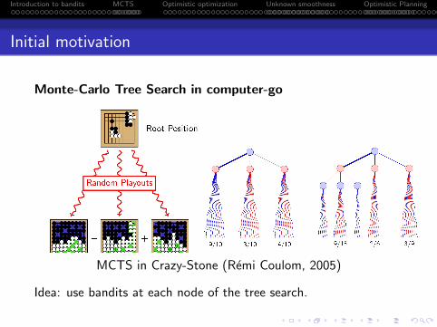
Initial motivation
Monte-Carlo Tree Search in computer-go
MCTS in Crazy-Stone (Remi Coulom, 2005)
Idea: use bandits at each node of the tree search.

. . . . . .
. . . . . . . . . . . . . . . . . . . . . . . . . . .Introduction to bandits
. . . . . .MCTS
. . . . . . . . . . . . . . . . . . . . . . . . . . . . . . . . . . .Optimistic optimization
. . . . . . . . . . . . . . . . . . . . . . . . . . . . . . .Unknown smoothness
. . . . . . . . . . . . . . . . . . .Optimistic Planning
Monte-Carlo Tree Search
Very efficient in several problems
Very inefficient in many other problems (even toy problems)
Not much theoretical guarantee...
We would like
Understand how the “optimism in the face of uncertainty”principle works in hierarchical problems
Define classes of problems for which variants of MCTS wouldbe efficient

. . . . . .
. . . . . . . . . . . . . . . . . . . . . . . . . . .Introduction to bandits
. . . . . .MCTS
. . . . . . . . . . . . . . . . . . . . . . . . . . . . . . . . . . .Optimistic optimization
. . . . . . . . . . . . . . . . . . . . . . . . . . . . . . .Unknown smoothness
. . . . . . . . . . . . . . . . . . .Optimistic Planning
Outline of this tutorial
...1 The stochastic multi-armed bandit
The K -armed bandit and UCBThe many-armed bandit
...2 Monte Carlo Tree Search
Bandits in a hierarchyComputer go and UCT
...3 Optimistic optimization with known smoothness
Deterministic rewardsStochastic rewards (X -armed bandit)
...4 Extension to unknown smoothness
...5 Optimistic planning
Deterministic dynamics,Open Loop planningMDPs with a model

. . . . . .
. . . . . . . . . . . . . . . . . . . . . . . . . . .Introduction to bandits
. . . . . .MCTS
. . . . . . . . . . . . . . . . . . . . . . . . . . . . . . . . . . .Optimistic optimization
. . . . . . . . . . . . . . . . . . . . . . . . . . . . . . .Unknown smoothness
. . . . . . . . . . . . . . . . . . .Optimistic Planning
Main message of this tutorial
The “optimism in the face of uncertainty” principle:
applies in a large class of decision making problems instochastic and deterministic environments
provides an efficient exploration of the search space byexploring the most promising areas first
provides a natural transition from global to local search
Performance depends on the “smoothness” of the functionaround the maximum w.r.t. some metric,
a measure of the quantity of near-optimal solutions,and our knowledge or not of this metric.

. . . . . .
. . . . . . . . . . . . . . . . . . . . . . . . . . .Introduction to bandits
. . . . . .MCTS
. . . . . . . . . . . . . . . . . . . . . . . . . . . . . . . . . . .Optimistic optimization
. . . . . . . . . . . . . . . . . . . . . . . . . . . . . . .Unknown smoothness
. . . . . . . . . . . . . . . . . . .Optimistic Planning
Multi-armed bandit
The multi-armed bandit problem
Setting:
Set of K arms (possible actions)
At each time t, choose an armIt ∈ 1, . . . ,K and receive a reward Xt
coming from arm It .
Goal: find an arm selection policy suchas to maximize a function of the rewards.
Exploration-exploitation tradeoff:
Exploit: act optimally according to our current beliefs
Explore: learn more about the environment
. . . . . .
. . . . . . . . . . . . . . . . . . . . . . . . . . .Introduction to bandits
. . . . . .MCTS
. . . . . . . . . . . . . . . . . . . . . . . . . . . . . . . . . . .Optimistic optimization
. . . . . . . . . . . . . . . . . . . . . . . . . . . . . . .Unknown smoothness
. . . . . . . . . . . . . . . . . . .Optimistic Planning
Multi-armed bandit
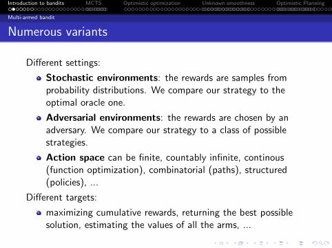
Numerous variants
Different settings:
Stochastic environments: the rewards are samples fromprobability distributions. We compare our strategy to theoptimal oracle one.
Adversarial environments: the rewards are chosen by anadversary. We compare our strategy to a class of possiblestrategies.
Action space can be finite, countably infinite, continous(function optimization), combinatorial (paths), structured(policies), ...
Different targets:
maximizing cumulative rewards, returning the best possiblesolution, estimating the values of all the arms, ...

. . . . . .
. . . . . . . . . . . . . . . . . . . . . . . . . . .Introduction to bandits
. . . . . .MCTS
. . . . . . . . . . . . . . . . . . . . . . . . . . . . . . . . . . .Optimistic optimization
. . . . . . . . . . . . . . . . . . . . . . . . . . . . . . .Unknown smoothness
. . . . . . . . . . . . . . . . . . .Optimistic Planning
Multi-armed bandit
Various applications
Clinical trials [Thompson 1933]
Ads placement on webpages
Nash equilibria (traffic or communication networks, agentsimulation, poker, ...)
Packet routing, itinerary selection, ...
Game-playing computers (Go, urban rivals, ...)
Optimization / planning given a finite numerical budget
. . . . . .
. . . . . . . . . . . . . . . . . . . . . . . . . . .Introduction to bandits
. . . . . .MCTS
. . . . . . . . . . . . . . . . . . . . . . . . . . . . . . . . . . .Optimistic optimization
. . . . . . . . . . . . . . . . . . . . . . . . . . . . . . .Unknown smoothness
. . . . . . . . . . . . . . . . . . .Optimistic Planning
Multi-armed bandit
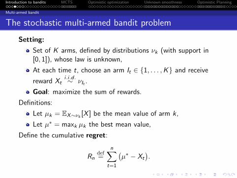
The stochastic multi-armed bandit problem
Setting:
Set of K arms, defined by distributions νk (with support in[0, 1]), whose law is unknown,
At each time t, choose an arm It ∈ 1, . . . ,K and receive
reward Xti .i .d .∼ νIt .
Goal: maximize the sum of rewards.
Definitions:
Let µk = EX∼νk [X ] be the mean value of arm k,
Let µ∗ = maxk µk the best mean value,
Define the cumulative regret:
Rndef=
n∑t=1
(µ∗ − Xt
).

. . . . . .
. . . . . . . . . . . . . . . . . . . . . . . . . . .Introduction to bandits
. . . . . .MCTS
. . . . . . . . . . . . . . . . . . . . . . . . . . . . . . . . . . .Optimistic optimization
. . . . . . . . . . . . . . . . . . . . . . . . . . . . . . .Unknown smoothness
. . . . . . . . . . . . . . . . . . .Optimistic Planning
Multi-armed bandit
The cumulative regret
The expected cumulative regret is
ERn = E[ n∑t=1
µ∗ − Xt
]= E
[E[ n∑t=1
µ∗ − Xt |It]]
= E[ n∑t=1
µ∗ − µIt
]= E
[ K∑k=1
(µ∗ − µk)n∑
t=1
1It = k]=
K∑k=1
∆kE[Tk(n)],
where ∆kdef= µ∗ − µk , and Tk(n) is the number of times arm k has
been pulled up to round n.Goal: Find an arm selection policy such as to minimize ERn.
. . . . . .
. . . . . . . . . . . . . . . . . . . . . . . . . . .Introduction to bandits
. . . . . .MCTS
. . . . . . . . . . . . . . . . . . . . . . . . . . . . . . . . . . .Optimistic optimization
. . . . . . . . . . . . . . . . . . . . . . . . . . . . . . .Unknown smoothness
. . . . . . . . . . . . . . . . . . .Optimistic Planning
Multi-armed bandit
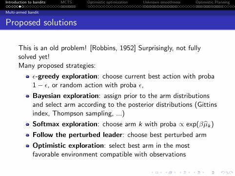
Proposed solutions
This is an old problem! [Robbins, 1952] Surprisingly, not fullysolved yet!Many proposed strategies:
ϵ-greedy exploration: choose current best action with proba1− ϵ, or random action with proba ϵ,
Bayesian exploration: assign prior to the arm distributionsand select arm according to the posterior distributions (Gittinsindex, Thompson sampling, ...)
Softmax exploration: choose arm k with proba ∝ exp(βµk)
Follow the perturbed leader: choose best perturbed arm
Optimistic exploration: select best arm in the mostfavorable environment compatible with observations

. . . . . .
. . . . . . . . . . . . . . . . . . . . . . . . . . .Introduction to bandits
. . . . . .MCTS
. . . . . . . . . . . . . . . . . . . . . . . . . . . . . . . . . . .Optimistic optimization
. . . . . . . . . . . . . . . . . . . . . . . . . . . . . . .Unknown smoothness
. . . . . . . . . . . . . . . . . . .Optimistic Planning
Multi-armed bandit
Optimism in the face of uncertainty
Follow the optimal policy in the most favorable environmentsamong all enviroments that are reasonably plausible given pastobservations
At time t, for each arm k, use past observations and someprobabilistic argument to define high-probability confidenceintervals containing the expected reward µk
The most favorable environment for arm k is thus the upperconfidence bound (UCB) on µk
Simple implementation: play the arm having the largest UCB!

. . . . . .
. . . . . . . . . . . . . . . . . . . . . . . . . . .Introduction to bandits
. . . . . .MCTS
. . . . . . . . . . . . . . . . . . . . . . . . . . . . . . . . . . .Optimistic optimization
. . . . . . . . . . . . . . . . . . . . . . . . . . . . . . .Unknown smoothness
. . . . . . . . . . . . . . . . . . .Optimistic Planning
UCB
The UCB1 algorithm [Auer, Cesa-Bianchi, Fischer, 2002]
Upper Confidence Bound algorithm: at each time t, select thearm with highest UCB:
Bk,tdef= µk,t +
√2 log(t)
Tk(t),
where:
µk,t =1
Tk (t)
∑ts=1 Xs1Is = k is the empirical mean of the
rewards received from arm k up to time t,
Tk(t) =∑t
s=1 1Is = k is the number of times arm k hasbeen pulled up to time t
Note that
Sum of an exploitation term and an exploration term.√2 log(t)Tk(t)
is a confidence interval term, so Bk,t is a UCB.

. . . . . .
. . . . . . . . . . . . . . . . . . . . . . . . . . .Introduction to bandits
. . . . . .MCTS
. . . . . . . . . . . . . . . . . . . . . . . . . . . . . . . . . . .Optimistic optimization
. . . . . . . . . . . . . . . . . . . . . . . . . . . . . . .Unknown smoothness
. . . . . . . . . . . . . . . . . . .Optimistic Planning
UCB
Intuition of the UCB algorithm
Idea:
The B-values Bk,t are h.p. UCBs on µk . Indeed we have:
P(|µk,t − µk | ≥
√2 log(t)
Tk(t)
)≤ 2
t2,
using a union bound for all possible values of Tk(t) ∈ 1, . . . , ttogether with Chernoff-Hoeffding’s inequality:
P(| 1m
m∑i=1
Yi − µ| ≥ ϵ)
≤ 2e−2mϵ2

. . . . . .
. . . . . . . . . . . . . . . . . . . . . . . . . . .Introduction to bandits
. . . . . .MCTS
. . . . . . . . . . . . . . . . . . . . . . . . . . . . . . . . . . .Optimistic optimization
. . . . . . . . . . . . . . . . . . . . . . . . . . . . . . .Unknown smoothness
. . . . . . . . . . . . . . . . . . .Optimistic Planning
UCB
Why does it make sense?
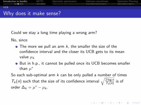
Could we stay a long time playing a wrong arm?
No, since
The more we pull an arm k , the smaller the size of theconfidence interval and the closer its UCB gets to its meanvalue µk
But in h.p., it cannot be pulled once its UCB becomes smallerthan µ∗
So each sub-optimal arm k can be only pulled a number of times
Tk(n) such that the size of its confidence interval√
2 log nTk(n)
is of
order ∆k = µ∗ − µk .
. . . . . .
. . . . . . . . . . . . . . . . . . . . . . . . . . .Introduction to bandits
. . . . . .MCTS
. . . . . . . . . . . . . . . . . . . . . . . . . . . . . . . . . . .Optimistic optimization
. . . . . . . . . . . . . . . . . . . . . . . . . . . . . . .Unknown smoothness
. . . . . . . . . . . . . . . . . . .Optimistic Planning
UCB
Why does it make sense?
Could we stay a long time playing a wrong arm?
No, since
The more we pull an arm k , the smaller the size of theconfidence interval and the closer its UCB gets to its meanvalue µk
But in h.p., it cannot be pulled once its UCB becomes smallerthan µ∗
So each sub-optimal arm k can be only pulled a number of times
Tk(n) such that the size of its confidence interval√
2 log nTk(n)
is of
order ∆k = µ∗ − µk .

. . . . . .
. . . . . . . . . . . . . . . . . . . . . . . . . . .Introduction to bandits
. . . . . .MCTS
. . . . . . . . . . . . . . . . . . . . . . . . . . . . . . . . . . .Optimistic optimization
. . . . . . . . . . . . . . . . . . . . . . . . . . . . . . .Unknown smoothness
. . . . . . . . . . . . . . . . . . .Optimistic Planning
UCB
Regret bound for UCB
.Proposition 1...
......
Each sub-optimal arm k is visited in average, at most:
ETk(n) ≤ 8log n
∆2k
+ 1 +π2
3
times (where ∆kdef= µ∗ − µk > 0).
.Theorem 1...
......
Thus the expected regret is bounded by:
ERn =∑k
E[Tk(n)]∆k ≤ 8∑
k:∆k>0
log n
∆k+ K (1 +
π2
3).

. . . . . .
. . . . . . . . . . . . . . . . . . . . . . . . . . .Introduction to bandits
. . . . . .MCTS
. . . . . . . . . . . . . . . . . . . . . . . . . . . . . . . . . . .Optimistic optimization
. . . . . . . . . . . . . . . . . . . . . . . . . . . . . . .Unknown smoothness
. . . . . . . . . . . . . . . . . . .Optimistic Planning
UCB
Intuition of the proof
Let k be a sub-optimal arm, and k∗ be an optimal arm. At time t,if arm k is selected, this means that
Bk,t ≥ Bk∗,t
µk,t +
√2 log(t)
Tk(t)≥ µk∗,t +
√2 log(t)
Tk∗(t)
µk + 2
√2 log(t)
Tk(t)≥ µ∗, with high proba
Tk(t) ≤ 8 log(t)
∆2k
Thus, if Tk(t) >8 log(t)∆2
k, then there is only a small probability that
arm k can be selected.

. . . . . .
. . . . . . . . . . . . . . . . . . . . . . . . . . .Introduction to bandits
. . . . . .MCTS
. . . . . . . . . . . . . . . . . . . . . . . . . . . . . . . . . . .Optimistic optimization
. . . . . . . . . . . . . . . . . . . . . . . . . . . . . . .Unknown smoothness
. . . . . . . . . . . . . . . . . . .Optimistic Planning
UCB
Proof of Proposition 1
Write u = 8 log(n)∆2
k+ 1. We have:
Tk(n) ≤ u +n∑
t=u+1
1It = k;Tk(t) > u
≤ u +n∑
t=u+1
[1µk,t − µk ≥
√2 log t
Tk(t)+ 1µk∗,t − µk ≤ −
√2 log t
Tk∗(t)]
Now, taking the expectation of both sides,
E[Tk(n)] ≤ u +n∑
t=u+1
2t−2
≤ 8 log(n)
∆2k
+ 1 +π2
3

. . . . . .
. . . . . . . . . . . . . . . . . . . . . . . . . . .Introduction to bandits
. . . . . .MCTS
. . . . . . . . . . . . . . . . . . . . . . . . . . . . . . . . . . .Optimistic optimization
. . . . . . . . . . . . . . . . . . . . . . . . . . . . . . .Unknown smoothness
. . . . . . . . . . . . . . . . . . .Optimistic Planning
Some variants
Better confidence bounds imply smaller regret
Chernoff-Hoeffding’s inequality 1/t-confidence bound:
EX ≤ 1
m
m∑i=1
Xi +
√log t
2m
Bernstein’s inequality:
EX ≤ 1
m
m∑i=1
Xi +
√2σ2 log t
m+
log t
3m
Empirical Bernstein’s inequality:
EX ≤ 1
m
m∑i=1
Xi +
√2σt
2 log(3t)
m+
8 log(3t)
3m
[Audibert, Munos, Szepesvari, 2007], [Maurer, Pontil, 2009]

. . . . . .
. . . . . . . . . . . . . . . . . . . . . . . . . . .Introduction to bandits
. . . . . .MCTS
. . . . . . . . . . . . . . . . . . . . . . . . . . . . . . . . . . .Optimistic optimization
. . . . . . . . . . . . . . . . . . . . . . . . . . . . . . .Unknown smoothness
. . . . . . . . . . . . . . . . . . .Optimistic Planning
Some variants
UCB-V
[Audibert, Munos, Szepesvari, 2007]
UCB using empirical variance estimate:
Bk,tdef= µk,t +
√2σk,t
2 log(1.2t)
Tk(t)+
3 log(1.2t)
Tk(t).
Then the expected regret is bounded as:
ERn ≤ 10( ∑
k:∆k>0
σ2k
∆k+ 2
)log(n).

. . . . . .
. . . . . . . . . . . . . . . . . . . . . . . . . . .Introduction to bandits
. . . . . .MCTS
. . . . . . . . . . . . . . . . . . . . . . . . . . . . . . . . . . .Optimistic optimization
. . . . . . . . . . . . . . . . . . . . . . . . . . . . . . .Unknown smoothness
. . . . . . . . . . . . . . . . . . .Optimistic Planning
Some variants
KL-UCB
[Garivier & Cappe, 2011] and [Maillard, Munos, Stoltz, 2011].For Bernoulli distributions, define the kl-UCB
Bk,tdef= sup
x ∈ [0, 1], kl(µk(t), x) ≤
log t
Tk(t)
Bk,t
kl(µk(t), x)
µk(t)
log tTk(t)
(non-asymptotic version of Sanov’s theorem)

. . . . . .
. . . . . . . . . . . . . . . . . . . . . . . . . . .Introduction to bandits
. . . . . .MCTS
. . . . . . . . . . . . . . . . . . . . . . . . . . . . . . . . . . .Optimistic optimization
. . . . . . . . . . . . . . . . . . . . . . . . . . . . . . .Unknown smoothness
. . . . . . . . . . . . . . . . . . .Optimistic Planning
Some variants
KL-UCB
The regret of KL-UCB is then bounded as
ERn =∑
k:∆k>0
∆k
kl(νk , ν∗)log n + o(log n).
This extends to several classes of distributions (one-dimensionalexponential family, finitely supported, ...)See also DMED [Honda, Takemura, 2010, 2011] and other relatedalgorithms.
Idea: Use the full empirical distribution to get a refined UCB.

. . . . . .
. . . . . . . . . . . . . . . . . . . . . . . . . . .Introduction to bandits
. . . . . .MCTS
. . . . . . . . . . . . . . . . . . . . . . . . . . . . . . . . . . .Optimistic optimization
. . . . . . . . . . . . . . . . . . . . . . . . . . . . . . .Unknown smoothness
. . . . . . . . . . . . . . . . . . .Optimistic Planning
Some variants
Lower bounds
For single-dimensional distributions [Lai, Robbins, 1985]:
lim infn→∞
ERn
log n≥
∑k:∆k>0
∆k
KL(νk , ν∗)
For larger class of distributions D [Burnetas, Katehakis, 1996]:
lim infn→∞
ERn
log n≥
∑k:∆k>0
∆k
Kinf(νk , µ∗),
where
Kinf(ν, µ)def= inf
KL(ν, ν ′) : ν ′ ∈ D and EX∼ν′ [X ] > µ
.

. . . . . .
. . . . . . . . . . . . . . . . . . . . . . . . . . .Introduction to bandits
. . . . . .MCTS
. . . . . . . . . . . . . . . . . . . . . . . . . . . . . . . . . . .Optimistic optimization
. . . . . . . . . . . . . . . . . . . . . . . . . . . . . . .Unknown smoothness
. . . . . . . . . . . . . . . . . . .Optimistic Planning
Some variants
Distribution-independent bound for UCB
Regret for UCB: ERn = O(log n∑
k =k∗1∆k
)
The smaller the gaps, the harder the problem (for large n)
For small n, the regret is trivially bounded by nmaxk ∆k
For small gaps it takes a long time to distinguish which arm is thebest..Proposition 2...
......
Distribution-independent bounds:
supDistributions
ERn ≤ 2
√2Kn
[log n + 1 +
π2
3
]
. . . . . .
. . . . . . . . . . . . . . . . . . . . . . . . . . .Introduction to bandits
. . . . . .MCTS
. . . . . . . . . . . . . . . . . . . . . . . . . . . . . . . . . . .Optimistic optimization
. . . . . . . . . . . . . . . . . . . . . . . . . . . . . . .Unknown smoothness
. . . . . . . . . . . . . . . . . . .Optimistic Planning
Some variants
Proof of the Proposition
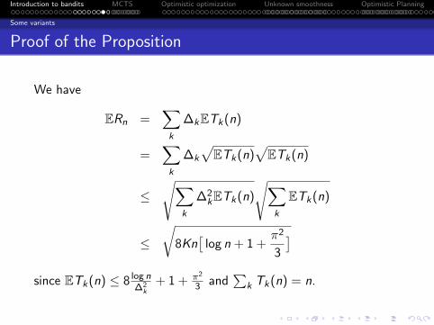
We have
ERn =∑k
∆kETk(n)
=∑k
∆k
√ETk(n)
√ETk(n)
≤√∑
k
∆2kETk(n)
√∑k
ETk(n)
≤√
8Kn[log n + 1 +
π2
3
]since ETk(n) ≤ 8 log n
∆2k+ 1 + π2
3 and∑
k Tk(n) = n.

. . . . . .
. . . . . . . . . . . . . . . . . . . . . . . . . . .Introduction to bandits
. . . . . .MCTS
. . . . . . . . . . . . . . . . . . . . . . . . . . . . . . . . . . .Optimistic optimization
. . . . . . . . . . . . . . . . . . . . . . . . . . . . . . .Unknown smoothness
. . . . . . . . . . . . . . . . . . .Optimistic Planning
Some variants
Distribution-independent bounds
We also have the lower bound [Cesa-Bianchi, Lugosi, 2006]:
infAlgo
supDistributions
ERn = Ω(√
Kn)
Notice that a refined algorithm (MOSS [Audibert, Bubeck, 2009])achieves the same order:
supDistributions
ERn = O(√
Kn).

. . . . . .
. . . . . . . . . . . . . . . . . . . . . . . . . . .Introduction to bandits
. . . . . .MCTS
. . . . . . . . . . . . . . . . . . . . . . . . . . . . . . . . . . .Optimistic optimization
. . . . . . . . . . . . . . . . . . . . . . . . . . . . . . .Unknown smoothness
. . . . . . . . . . . . . . . . . . .Optimistic Planning
Many-armed bandits
Many-armed bandits: an example
There is a countably infinite number of arms.
Unstructured set of actions: The rewards received so far do nottell us anything about the value of unobserved arms.
Example: Each day, select a restaurant:
among the ones where you have already been
because it is good (Exploitation)or not well known (Exploration)
or choose a new one randomly (Discovery)
Other examples: Marketing (ex: sending catalogues), mining forvaluable resources, ...

. . . . . .
. . . . . . . . . . . . . . . . . . . . . . . . . . .Introduction to bandits
. . . . . .MCTS
. . . . . . . . . . . . . . . . . . . . . . . . . . . . . . . . . . .Optimistic optimization
. . . . . . . . . . . . . . . . . . . . . . . . . . . . . . .Unknown smoothness
. . . . . . . . . . . . . . . . . . .Optimistic Planning
Many-armed bandits
Many-armed bandits: Assumptions
We make a (probabilistic) assumption about the mean-value of anynew arm.
Usual assumption: the distribution of the mean-reward of anew arm is known [Banks, Sundaram, 1992], [Berry, Chen,Zame, Heath, Shepp, 1997].
Much weaker assumption: Assume we know β > 0 suchthat
P(µ(new arm) > µ∗ − ϵ) = Θ(ϵβ),
β characterizes the probability of selecting near-optimal arms
Large β =⇒ small chance of pulling good arm, thus oneneeds to pull many arms. And vice-versa.

. . . . . .
. . . . . . . . . . . . . . . . . . . . . . . . . . .Introduction to bandits
. . . . . .MCTS
. . . . . . . . . . . . . . . . . . . . . . . . . . . . . . . . . . .Optimistic optimization
. . . . . . . . . . . . . . . . . . . . . . . . . . . . . . .Unknown smoothness
. . . . . . . . . . . . . . . . . . .Optimistic Planning
Many-armed bandits
UCB with Arm Increasing Rule [Wang, Audibert, Munos, 2008]
K(t) played arms Arms not played yet
UCB-AIR:
K (0) = 0. At time t + 1, pull a new arm if
K (t) <
tβ2 if β < 1 and µ∗ < 1
tβ
β+1 if β ≥ 1 or µ∗ = 1
Otherwise, apply UCB–V on the K (t) current arms, i.e., play
argmax1≤k≤K(t)
µk,t︸︷︷︸empirical rewards
+
√2Vk,tEtTk(t)
+3EtTk(t)︸ ︷︷ ︸
Confidence interval
,
with exploration sequence: c log(log t) ≤ Et ≤ log t.
. . . . . .
. . . . . . . . . . . . . . . . . . . . . . . . . . .Introduction to bandits
. . . . . .MCTS
. . . . . . . . . . . . . . . . . . . . . . . . . . . . . . . . . . .Optimistic optimization
. . . . . . . . . . . . . . . . . . . . . . . . . . . . . . .Unknown smoothness
. . . . . . . . . . . . . . . . . . .Optimistic Planning
Many-armed bandits
Regret analysis of UCB-AIR
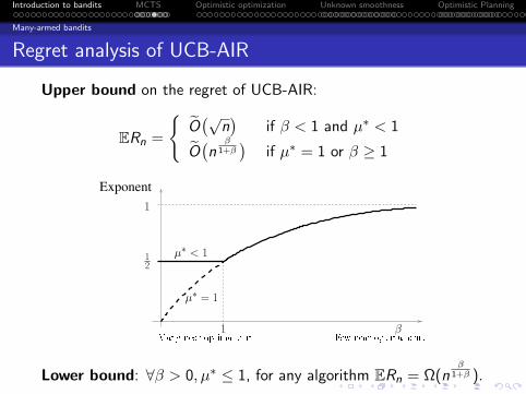
Upper bound on the regret of UCB-AIR:
ERn =
O(√
n)
if β < 1 and µ∗ < 1
O(n
β1+β
)if µ∗ = 1 or β ≥ 1
Exponent
1
1
2
µ∗ < 1
1 βMany near-optimal arms Few near-optimal arms
µ∗ = 1
Lower bound: ∀β > 0, µ∗ ≤ 1, for any algorithm ERn = Ω(nβ
1+β ).

. . . . . .
. . . . . . . . . . . . . . . . . . . . . . . . . . .Introduction to bandits
. . . . . .MCTS
. . . . . . . . . . . . . . . . . . . . . . . . . . . . . . . . . . .Optimistic optimization
. . . . . . . . . . . . . . . . . . . . . . . . . . . . . . .Unknown smoothness
. . . . . . . . . . . . . . . . . . .Optimistic Planning
Many-armed bandits
Remarks and possible extensions
Remarks
When β > 1 or µ∗ = 1 the upper and lower bounds match (upto logarithmic factor).
Exploration-Exploitation-Discovery tradeoff:
Exploitation: Pull a good armExploration: Pull an uncertain armDiscovery: Pull a new arm
The exploration sequence Et can be of order log log t (insteadof log t): discovery replaces exploration
Open question: similar performance when β is unknown?(i.e. adaptive strategy that estimates β while minimizingregret).

. . . . . .
. . . . . . . . . . . . . . . . . . . . . . . . . . .Introduction to bandits
. . . . . .MCTS
. . . . . . . . . . . . . . . . . . . . . . . . . . . . . . . . . . .Optimistic optimization
. . . . . . . . . . . . . . . . . . . . . . . . . . . . . . .Unknown smoothness
. . . . . . . . . . . . . . . . . . .Optimistic Planning
Many-armed bandits
Bandits with a structured set of actions
Optimism in the face of uncertainty extends to:
Linear bandits [Auer, 2002], [Dani, Hayes, Kakade, 2008], [Abbasi-Yadkori, 2009],
[Rusmevichientong, Tsitsiklis, 2010], [Filippi, Cappe, Garivier, Szepesvari, 2010]
Convex bandits [Zinkevich, 2003], [Flaxman, Kalai, McMahan, 2005], [Hazan, Agarwal, Kale,
2006], [Bartlett, Hazan, Rakhlin, 2007], [Shalev-Shwartz, 2007], [Abernethy, Bartlett, Rakhlin, Tewari,
2008], [Narayanan, Rakhlin, 2010]
Lipschitz bandits [Agrawal, 1995], [Kleinberg, 2004], [Auer, Ortner, Szepesvari, 2007],
[Kleinberg, Slivkins, Upfall, 2008], [Bubeck, Munos, Stoltz, Szepesvari, 2011]
Gaussian bandits [Dorard, Glowacka, Shawe-Taylor, 2009], [Grunewalder, Audibert, Opper,
Shawe-Taylor, 2010], [Srinivas, Krause, Kakade, Seeger, 2010]
Contextual bandits [Woodroofe, 1979], [Auer, 2002], [Wang, Kulkarni, Poor, 2005], [Pandey,
Agarwal, Chakrabarti, Josifovski, 2007], [Langford, Zhang, 2007], [Hazan, Megiddo, 2007], [Rigollet, Zeevi,
2010], [Chu, Li, Reyzin, Schapire, 2011], [Slivkins, 2011]
MDPs [Burnetas, Katehakis, 1997], [Jaksch, Ortner, Auer, 2010], [Bartlett, Tewari, 2009]
Combinatorial bandits [Cesa-Bianchi, Lugosi, 2009], [Audibert, Bubeck, Lugosi, 2011]

. . . . . .
. . . . . . . . . . . . . . . . . . . . . . . . . . .Introduction to bandits
. . . . . .MCTS
. . . . . . . . . . . . . . . . . . . . . . . . . . . . . . . . . . .Optimistic optimization
. . . . . . . . . . . . . . . . . . . . . . . . . . . . . . .Unknown smoothness
. . . . . . . . . . . . . . . . . . .Optimistic Planning
Bandits in a hierarchy
Bandit = tool to rapidly select the right action, given noisyestimate of their value
Serve as building block for more complex problems
Hierarchy of bandits: The reward obtained when pulling anarm is itself the return of another bandit in a hierarchy.
Illustration: Monte-Carlo Tree Search in computer-go.
. . . . . .
. . . . . . . . . . . . . . . . . . . . . . . . . . .Introduction to bandits
. . . . . .MCTS
. . . . . . . . . . . . . . . . . . . . . . . . . . . . . . . . . . .Optimistic optimization
. . . . . . . . . . . . . . . . . . . . . . . . . . . . . . .Unknown smoothness
. . . . . . . . . . . . . . . . . . .Optimistic Planning
computer go
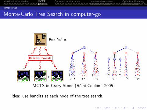
Monte-Carlo Tree Search in computer-go
MCTS in Crazy-Stone (Remi Coulom, 2005)
Idea: use bandits at each node of the tree search.

. . . . . .
. . . . . . . . . . . . . . . . . . . . . . . . . . .Introduction to bandits
. . . . . .MCTS
. . . . . . . . . . . . . . . . . . . . . . . . . . . . . . . . . . .Optimistic optimization
. . . . . . . . . . . . . . . . . . . . . . . . . . . . . . .Unknown smoothness
. . . . . . . . . . . . . . . . . . .Optimistic Planning
computer go
Hierarchical bandit algorithm
Upper Confidence Bound(UCB) algo at each node
Bj(t)def= µj(t) +
√2 log(t)
Tj(t).
Intuition:- Explore first the mostpromising branches- Average converges to max
Node i: Bi
Bj
Adaptive Multistage Sampling (AMS) algorithm [Chang, Fu,Hu, Marcus, 2005]
UCB applied to Trees (UCT) [Kocsis and Szepesvari, 2006]
. . . . . .
. . . . . . . . . . . . . . . . . . . . . . . . . . .Introduction to bandits
. . . . . .MCTS
. . . . . . . . . . . . . . . . . . . . . . . . . . . . . . . . . . .Optimistic optimization
. . . . . . . . . . . . . . . . . . . . . . . . . . . . . . .Unknown smoothness
. . . . . . . . . . . . . . . . . . .Optimistic Planning
computer go
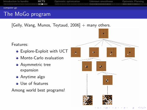
The MoGo program
[Gelly, Wang, Munos, Teytaud, 2006] + many others.
Features:
Explore-Exploit with UCT
Monte-Carlo evaluation
Asymmetric treeexpansion
Anytime algo
Use of features
Among world best programs!
. . . . . .
. . . . . . . . . . . . . . . . . . . . . . . . . . .Introduction to bandits
. . . . . .MCTS
. . . . . . . . . . . . . . . . . . . . . . . . . . . . . . . . . . .Optimistic optimization
. . . . . . . . . . . . . . . . . . . . . . . . . . . . . . .Unknown smoothness
. . . . . . . . . . . . . . . . . . .Optimistic Planning
UCT
Asymptotic analysis of UCT
[Kocsis and Szepesvari, 2006]
In a tree with finite depth, all leaves will be eventuallyexplored an infinite number of times, thus by backwardinduction, UCT is consistent and the regret is O(log n).
However, the constant can be so bad that there is notfinite-time guarantee for any reasonable n.

. . . . . .
. . . . . . . . . . . . . . . . . . . . . . . . . . .Introduction to bandits
. . . . . .MCTS
. . . . . . . . . . . . . . . . . . . . . . . . . . . . . . . . . . .Optimistic optimization
. . . . . . . . . . . . . . . . . . . . . . . . . . . . . . .Unknown smoothness
. . . . . . . . . . . . . . . . . . .Optimistic Planning
UCT
Bad example for UCT
1
D
D−1
D
D−2
D
D−3
D10
depth D
The left branches are explored exponentially more often than theright ones.

. . . . . .
. . . . . . . . . . . . . . . . . . . . . . . . . . .Introduction to bandits
. . . . . .MCTS
. . . . . . . . . . . . . . . . . . . . . . . . . . . . . . . . . . .Optimistic optimization
. . . . . . . . . . . . . . . . . . . . . . . . . . . . . . .Unknown smoothness
. . . . . . . . . . . . . . . . . . .Optimistic Planning
UCT
Finite-time analysis of UCT
The regret is disastrous: (see [Coquelin and Munos, 2007])
ERn = Ω(exp(exp(. . . exp(︸ ︷︷ ︸D times
1) . . . ))) + O(log(n)),
whereas a uniform exploration of the tree would be “only”exponential in D.
Problem: at each node, the rewards are not i.i.d.=⇒ the B-values are not UCBs.
UCT implicitely makes the assumption that the underlying functionis very smooth.Problems:
Can we recover the optimistic principle?
How should we define the smoothness of a function?

. . . . . .
. . . . . . . . . . . . . . . . . . . . . . . . . . .Introduction to bandits
. . . . . .MCTS
. . . . . . . . . . . . . . . . . . . . . . . . . . . . . . . . . . .Optimistic optimization
. . . . . . . . . . . . . . . . . . . . . . . . . . . . . . .Unknown smoothness
. . . . . . . . . . . . . . . . . . .Optimistic Planning
Illustration
Optimization of a deterministic Lipschitz function
Problem: Find online the maximum of f : X → IR, assumed to beLipschitz:
|f (x)− f (y)| ≤ ℓ(x , y).
Protocol:
For each time step t = 1, 2, . . . , n select a state xt ∈ X
Observe f (xt)
Return a state x(n)
Performance assessed in terms of the simple regret
rn = f ∗ − f (x(n)),
where f ∗ = supx∈X f (x).
. . . . . .
. . . . . . . . . . . . . . . . . . . . . . . . . . .Introduction to bandits
. . . . . .MCTS
. . . . . . . . . . . . . . . . . . . . . . . . . . . . . . . . . . .Optimistic optimization
. . . . . . . . . . . . . . . . . . . . . . . . . . . . . . .Unknown smoothness
. . . . . . . . . . . . . . . . . . .Optimistic Planning
Illustration
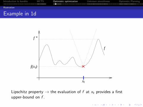
Example in 1d
f(x )t
xt
f
f *
Lipschitz property → the evaluation of f at xt provides a firstupper-bound on f .

. . . . . .
. . . . . . . . . . . . . . . . . . . . . . . . . . .Introduction to bandits
. . . . . .MCTS
. . . . . . . . . . . . . . . . . . . . . . . . . . . . . . . . . . .Optimistic optimization
. . . . . . . . . . . . . . . . . . . . . . . . . . . . . . .Unknown smoothness
. . . . . . . . . . . . . . . . . . .Optimistic Planning
Illustration
Example in 1d (continued)
New point → refined upper-bound on f .

. . . . . .
. . . . . . . . . . . . . . . . . . . . . . . . . . .Introduction to bandits
. . . . . .MCTS
. . . . . . . . . . . . . . . . . . . . . . . . . . . . . . . . . . .Optimistic optimization
. . . . . . . . . . . . . . . . . . . . . . . . . . . . . . .Unknown smoothness
. . . . . . . . . . . . . . . . . . .Optimistic Planning
Illustration
Example in 1d (continued)
Question: where should one sample the next point?Answer: select the point with highest upper bound!“Optimism in the face of (partial observation) uncertainty”

. . . . . .
. . . . . . . . . . . . . . . . . . . . . . . . . . .Introduction to bandits
. . . . . .MCTS
. . . . . . . . . . . . . . . . . . . . . . . . . . . . . . . . . . .Optimistic optimization
. . . . . . . . . . . . . . . . . . . . . . . . . . . . . . .Unknown smoothness
. . . . . . . . . . . . . . . . . . .Optimistic Planning
Illustration
Several issues
...1 Lipschitz assumption is quite strong
...2 Finding the optimum of the upper-bounding function may behard!
...3 How to handle noise?

. . . . . .
. . . . . . . . . . . . . . . . . . . . . . . . . . .Introduction to bandits
. . . . . .MCTS
. . . . . . . . . . . . . . . . . . . . . . . . . . . . . . . . . . .Optimistic optimization
. . . . . . . . . . . . . . . . . . . . . . . . . . . . . . .Unknown smoothness
. . . . . . . . . . . . . . . . . . .Optimistic Planning
DOO
Local smoothness property
Assumption: f is “locally smooth” around its max. w.r.t. ℓ...1 X is equipped with a semi-metric ℓ: ℓ is symmetric, andℓ(x , y) = 0 ⇔ x = y .
...2 For all x ∈ X ,f (x∗)− f (x) ≤ ℓ(x , x∗).

. . . . . .
. . . . . . . . . . . . . . . . . . . . . . . . . . .Introduction to bandits
. . . . . .MCTS
. . . . . . . . . . . . . . . . . . . . . . . . . . . . . . . . . . .Optimistic optimization
. . . . . . . . . . . . . . . . . . . . . . . . . . . . . . .Unknown smoothness
. . . . . . . . . . . . . . . . . . .Optimistic Planning
DOO
Local smoothness property
x∗ X
f(x∗) f
f(x∗)− ℓ(x, x∗)
For all x ∈ X ,f (x) ≥ f (x∗)− ℓ(x , x∗).

. . . . . .
. . . . . . . . . . . . . . . . . . . . . . . . . . .Introduction to bandits
. . . . . .MCTS
. . . . . . . . . . . . . . . . . . . . . . . . . . . . . . . . . . .Optimistic optimization
. . . . . . . . . . . . . . . . . . . . . . . . . . . . . . .Unknown smoothness
. . . . . . . . . . . . . . . . . . .Optimistic Planning
DOO
Local smoothness is enough!
x∗
f(x∗)
f
Optimistic principle only requires:
a true bound at the maximum
the bounds gets refined when adding more points

. . . . . .
. . . . . . . . . . . . . . . . . . . . . . . . . . .Introduction to bandits
. . . . . .MCTS
. . . . . . . . . . . . . . . . . . . . . . . . . . . . . . . . . . .Optimistic optimization
. . . . . . . . . . . . . . . . . . . . . . . . . . . . . . .Unknown smoothness
. . . . . . . . . . . . . . . . . . .Optimistic Planning
DOO
Efficient implementation
Deterministic Optimistic Optimization (DOO) builds anadaptive partitioning of the domain where cells are refinedaccording to their upper bounds.
For t = 1 to n,
Let Tt be the current partition with cells Xi
Define an upper bound for each cell:
Bi = f (xi ) + diam(Xi ),
where xi ∈ Xi and diam(Xi )def= supx,y∈Xi
ℓ(x , y)Select the cell with highest bound
It = argmaxi
Bi .
Expand It : refine the grid and evaluate f in children cells
Return x(n)def= argmaxxt1≤t≤n
f (xt)

. . . . . .
. . . . . . . . . . . . . . . . . . . . . . . . . . .Introduction to bandits
. . . . . .MCTS
. . . . . . . . . . . . . . . . . . . . . . . . . . . . . . . . . . .Optimistic optimization
. . . . . . . . . . . . . . . . . . . . . . . . . . . . . . .Unknown smoothness
. . . . . . . . . . . . . . . . . . .Optimistic Planning
DOO
Properties of DOO
At any time t, let Xi∗ be the cell containing x∗ and xi∗ ∈ Xi∗
the point where the function has been evaluated. Then
f (x∗) ≤ f (xi∗) + ℓ(x∗, xi∗) ≤ f (xi∗) + diam(Xi∗) = Bi∗
Thus any suboptimal cell Xi such that
f (xi ) + diam(Xi ) < f (x∗)
will never be expanded.
Thus finite-time performance guarantees can be obtained.
. . . . . .
. . . . . . . . . . . . . . . . . . . . . . . . . . .Introduction to bandits
. . . . . .MCTS
. . . . . . . . . . . . . . . . . . . . . . . . . . . . . . . . . . .Optimistic optimization
. . . . . . . . . . . . . . . . . . . . . . . . . . . . . . .Unknown smoothness
. . . . . . . . . . . . . . . . . . .Optimistic Planning
DOO
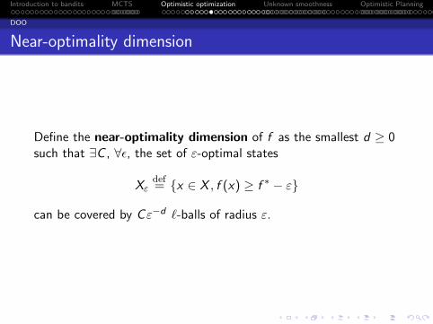
Near-optimality dimension
Define the near-optimality dimension of f as the smallest d ≥ 0such that ∃C , ∀ϵ, the set of ε-optimal states
Xεdef= x ∈ X , f (x) ≥ f ∗ − ε
can be covered by Cε−d ℓ-balls of radius ε.

. . . . . .
. . . . . . . . . . . . . . . . . . . . . . . . . . .Introduction to bandits
. . . . . .MCTS
. . . . . . . . . . . . . . . . . . . . . . . . . . . . . . . . . . .Optimistic optimization
. . . . . . . . . . . . . . . . . . . . . . . . . . . . . . .Unknown smoothness
. . . . . . . . . . . . . . . . . . .Optimistic Planning
DOO
Example 1:
Assume the function is piecewise linear at its maximum:
f (x∗)− f (x) = Θ(||x∗ − x ||).
ε
ε
Using ℓ(x , y) = ∥x − y∥, it takes O(ϵ0) balls of radius ϵ to coverXε. Thus d = 0.

. . . . . .
. . . . . . . . . . . . . . . . . . . . . . . . . . .Introduction to bandits
. . . . . .MCTS
. . . . . . . . . . . . . . . . . . . . . . . . . . . . . . . . . . .Optimistic optimization
. . . . . . . . . . . . . . . . . . . . . . . . . . . . . . .Unknown smoothness
. . . . . . . . . . . . . . . . . . .Optimistic Planning
DOO
Example 2:
Assume the function is locally quadratic around its maximum:
f (x∗)− f (x) = Θ(||x∗ − x ||2).
ε
εf
f(x∗)− ‖x− x∗‖
For ℓ(x , y) = ||x − y ||, it takes O(ϵ−D/2) balls of radius ϵ to coverXε (of size O(ϵD/2)). Thus d = D/2.

. . . . . .
. . . . . . . . . . . . . . . . . . . . . . . . . . .Introduction to bandits
. . . . . .MCTS
. . . . . . . . . . . . . . . . . . . . . . . . . . . . . . . . . . .Optimistic optimization
. . . . . . . . . . . . . . . . . . . . . . . . . . . . . . .Unknown smoothness
. . . . . . . . . . . . . . . . . . .Optimistic Planning
DOO
Example 2:
Assume the function is locally quadratic around its maximum:
f (x∗)− f (x) = Θ(||x∗ − x ||2)
ε
ε
f
f(x∗)− ‖x− x∗‖2
For ℓ(x , y) = ||x − y ||2, it takes O(ϵ0) ℓ-balls of radius ϵ to coverXε. Thus d = 0.
. . . . . .
. . . . . . . . . . . . . . . . . . . . . . . . . . .Introduction to bandits
. . . . . .MCTS
. . . . . . . . . . . . . . . . . . . . . . . . . . . . . . . . . . .Optimistic optimization
. . . . . . . . . . . . . . . . . . . . . . . . . . . . . . .Unknown smoothness
. . . . . . . . . . . . . . . . . . .Optimistic Planning
DOO
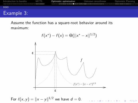
Example 3:
Assume the function has a square-root behavior around itsmaximum:
f (x∗)− f (x) = Θ(||x∗ − x ||1/2)
ε
ε
f
f(x∗)− ‖x− x∗‖1/2
For ℓ(x , y) = ∥x − y∥1/2 we have d = 0.

. . . . . .
. . . . . . . . . . . . . . . . . . . . . . . . . . .Introduction to bandits
. . . . . .MCTS
. . . . . . . . . . . . . . . . . . . . . . . . . . . . . . . . . . .Optimistic optimization
. . . . . . . . . . . . . . . . . . . . . . . . . . . . . . .Unknown smoothness
. . . . . . . . . . . . . . . . . . .Optimistic Planning
DOO
Example 4:
Assume X = [0, 1]D and f is locally equivalent to a polynomial ofdegree α > 0 around its maximum (i.e. f is α-smooth):
f (x∗)− f (x) = Θ(||x∗ − x ||α)
Consider the semi-metric ℓ(x , y) = ∥x − y∥β, for some β > 0.
If α = β, then d = 0.
If α > β, then d = D( 1β − 1α) > 0.
If α < β, then the function is not locally smooth wrt ℓ.
. . . . . .
. . . . . . . . . . . . . . . . . . . . . . . . . . .Introduction to bandits
. . . . . .MCTS
. . . . . . . . . . . . . . . . . . . . . . . . . . . . . . . . . . .Optimistic optimization
. . . . . . . . . . . . . . . . . . . . . . . . . . . . . . .Unknown smoothness
. . . . . . . . . . . . . . . . . . .Optimistic Planning
DOO
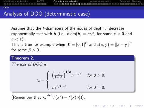
Analysis of DOO (deterministic case)
Assume that the ℓ-diameters of the nodes of depth h decreaseexponentially fast with h (i.e., diam(h) = cγh, for some c > 0 andγ < 1).This is true for example when X = [0, 1]D and ℓ(x , y) = ∥x − y∥βfor some β > 0..Theorem 2...
......
The loss of DOO is
rn =
(
C1−γd
)1/dn−1/d for d > 0,
cγn/C−1 for d = 0.
(Remember that rndef= f (x∗)− f (x(n))).
. . . . . .
. . . . . . . . . . . . . . . . . . . . . . . . . . .Introduction to bandits
. . . . . .MCTS
. . . . . . . . . . . . . . . . . . . . . . . . . . . . . . . . . . .Optimistic optimization
. . . . . . . . . . . . . . . . . . . . . . . . . . . . . . .Unknown smoothness
. . . . . . . . . . . . . . . . . . .Optimistic Planning
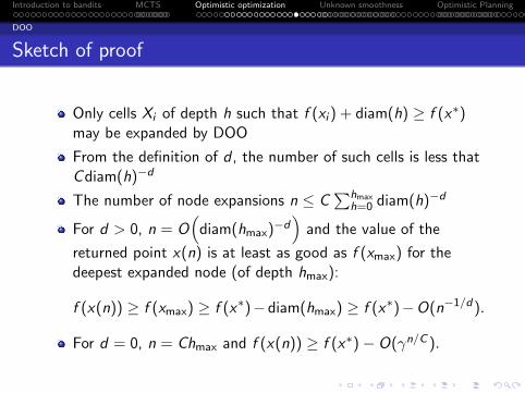
DOO
Sketch of proof
Only cells Xi of depth h such that f (xi ) + diam(h) ≥ f (x∗)may be expanded by DOO
From the definition of d , the number of such cells is less thatCdiam(h)−d
The number of node expansions n ≤ C∑hmax
h=0 diam(h)−d
For d > 0, n = O(diam(hmax)
−d)and the value of the
returned point x(n) is at least as good as f (xmax) for thedeepest expanded node (of depth hmax):
f (x(n)) ≥ f (xmax) ≥ f (x∗)−diam(hmax) ≥ f (x∗)−O(n−1/d).
For d = 0, n = Chmax and f (x(n)) ≥ f (x∗)− O(γn/C ).

. . . . . .
. . . . . . . . . . . . . . . . . . . . . . . . . . .Introduction to bandits
. . . . . .MCTS
. . . . . . . . . . . . . . . . . . . . . . . . . . . . . . . . . . .Optimistic optimization
. . . . . . . . . . . . . . . . . . . . . . . . . . . . . . .Unknown smoothness
. . . . . . . . . . . . . . . . . . .Optimistic Planning
DOO
About the local smoothness assumption
Assume f satisfies f (x∗)− f (x) = Θ(||x∗ − x ||α).
Use DOO with the semi-metric ℓ(x , y) = ∥x − y∥β:If α = β, then d = 0: the true “local smoothness” of thefunction is known, and exponential rate is achieved.
If α > β, then d = D( 1β − 1α) > 0: we under-estimate the
smoothness, which causes more exploration than needed.
If α < β: We over-estimate the true smoothness and DOOmay fail to find the global optimum.
The performance of DOO heavilly relies on our knowledge of thetrue local smoothness.

. . . . . .
. . . . . . . . . . . . . . . . . . . . . . . . . . .Introduction to bandits
. . . . . .MCTS
. . . . . . . . . . . . . . . . . . . . . . . . . . . . . . . . . . .Optimistic optimization
. . . . . . . . . . . . . . . . . . . . . . . . . . . . . . .Unknown smoothness
. . . . . . . . . . . . . . . . . . .Optimistic Planning
DOO
Experiments [1]
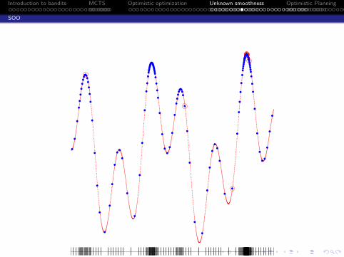
f (x) = 12(sin(13x) sin(27x) + 1) satisfies the local smoothness
assumption f (x) ≥ f (x∗)− ℓ(x , x∗) with
ℓ1(x , y) = 14|x − y | (i.e., f is globally Lipschitz),ℓ2(x , y) = 222|x − y |2 (i.e., f is locally quadratic).

. . . . . .
. . . . . . . . . . . . . . . . . . . . . . . . . . .Introduction to bandits
. . . . . .MCTS
. . . . . . . . . . . . . . . . . . . . . . . . . . . . . . . . . . .Optimistic optimization
. . . . . . . . . . . . . . . . . . . . . . . . . . . . . . .Unknown smoothness
. . . . . . . . . . . . . . . . . . .Optimistic Planning
DOO
Experiments [2]
Using ℓ1(x , y) = 14|x − y | (i.e., f is globally Lipschitz). n = 150.
The trees Tn built by DOO after n = 150 evaluations.
. . . . . .
. . . . . . . . . . . . . . . . . . . . . . . . . . .Introduction to bandits
. . . . . .MCTS
. . . . . . . . . . . . . . . . . . . . . . . . . . . . . . . . . . .Optimistic optimization
. . . . . . . . . . . . . . . . . . . . . . . . . . . . . . .Unknown smoothness
. . . . . . . . . . . . . . . . . . .Optimistic Planning
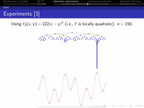
DOO
Experiments [3]
Using ℓ2(x , y) = 222|x − y |2 (i.e., f is locally quadratic). n = 150.
The trees Tn built by DOO after n = 150 evaluations.

. . . . . .
. . . . . . . . . . . . . . . . . . . . . . . . . . .Introduction to bandits
. . . . . .MCTS
. . . . . . . . . . . . . . . . . . . . . . . . . . . . . . . . . . .Optimistic optimization
. . . . . . . . . . . . . . . . . . . . . . . . . . . . . . .Unknown smoothness
. . . . . . . . . . . . . . . . . . .Optimistic Planning
DOO
Experiments [4]
n uniform grid DOO with ℓ1 (d = 1/2) DOO with ℓ2 (d = 0)
50 1.25× 10⁻² 2.53× 10⁻⁵ 1.20× 10⁻²
100 8.31× 10⁻³ 2.53× 10⁻⁵ 1.67× 10⁻⁷
150 9.72× 10⁻³ 4.93× 10⁻⁶ 4.44× 10⁻¹⁶
Loss rn for different values of n for a uniform grid and DOO withthe two semi-metric ℓ1 and ℓ2.

. . . . . .
. . . . . . . . . . . . . . . . . . . . . . . . . . .Introduction to bandits
. . . . . .MCTS
. . . . . . . . . . . . . . . . . . . . . . . . . . . . . . . . . . .Optimistic optimization
. . . . . . . . . . . . . . . . . . . . . . . . . . . . . . .Unknown smoothness
. . . . . . . . . . . . . . . . . . .Optimistic Planning
X -armed bandits
How to handle noise?
The evaluation of f at xt is perturbed by noise:
rt = f (xt) + ϵt , with E[ϵt |xt ] = 0.
f(x )t
xt
f
f *

. . . . . .
. . . . . . . . . . . . . . . . . . . . . . . . . . .Introduction to bandits
. . . . . .MCTS
. . . . . . . . . . . . . . . . . . . . . . . . . . . . . . . . . . .Optimistic optimization
. . . . . . . . . . . . . . . . . . . . . . . . . . . . . . .Unknown smoothness
. . . . . . . . . . . . . . . . . . .Optimistic Planning
X -armed bandits
Where should one sample next?
x
How to define a high probability upper bound at any state x?

. . . . . .
. . . . . . . . . . . . . . . . . . . . . . . . . . .Introduction to bandits
. . . . . .MCTS
. . . . . . . . . . . . . . . . . . . . . . . . . . . . . . . . . . .Optimistic optimization
. . . . . . . . . . . . . . . . . . . . . . . . . . . . . . .Unknown smoothness
. . . . . . . . . . . . . . . . . . .Optimistic Planning
X -armed bandits
UCB in a given cell
xt
f(xt)
rt
x
For a fixed domain Xi ∋ x containing Ti points xt ∈ Xi , we have
that∑Ti
t=1 rt − f (xt) is a Martingale. Thus by Azuma’s inequality,with 1/n-confidence,
1
Ti
Ti∑t=1
rt +
√log n
2Ti≥ 1
Ti
Ti∑t=1
f (xt).

. . . . . .
. . . . . . . . . . . . . . . . . . . . . . . . . . .Introduction to bandits
. . . . . .MCTS
. . . . . . . . . . . . . . . . . . . . . . . . . . . . . . . . . . .Optimistic optimization
. . . . . . . . . . . . . . . . . . . . . . . . . . . . . . .Unknown smoothness
. . . . . . . . . . . . . . . . . . .Optimistic Planning
X -armed bandits
UCB in a given cell
For an optimal cell Xi ∋ x∗ containing Ti points xt ∈ Xi ,
we have
1
Ti
Ti∑t=1
f (xt) ≥ f (x∗)− 1
Ti
Ti∑t=1
ℓ(xt , x∗) ≥ f (x∗)− diam(Xi ).
(where we used f (xt) ≥ f (x∗)− ℓ(xt , x∗))
Thus
1
Ti
Ti∑t=1
rt +
√log n
2Ti+ diam(Xi ) ≥ f (x∗).

. . . . . .
. . . . . . . . . . . . . . . . . . . . . . . . . . .Introduction to bandits
. . . . . .MCTS
. . . . . . . . . . . . . . . . . . . . . . . . . . . . . . . . . . .Optimistic optimization
. . . . . . . . . . . . . . . . . . . . . . . . . . . . . . .Unknown smoothness
. . . . . . . . . . . . . . . . . . .Optimistic Planning
X -armed bandits
Upper confidence bound
diam(Xi)
Upper-bound
x
√
logn
2Ti
1
Ti
∑
Ti
t=1 rt
In any cell Xi define the UCB:1
Ti
Ti∑t=1
rt +
√log n
2Ti+ diam(Xi ).
Tradeoff between size of the confidence interval and diameter.Considering several domains we can derive a tighter UCB

. . . . . .
. . . . . . . . . . . . . . . . . . . . . . . . . . .Introduction to bandits
. . . . . .MCTS
. . . . . . . . . . . . . . . . . . . . . . . . . . . . . . . . . . .Optimistic optimization
. . . . . . . . . . . . . . . . . . . . . . . . . . . . . . .Unknown smoothness
. . . . . . . . . . . . . . . . . . .Optimistic Planning
X -armed bandits
Optimistic principle for X -armed bandits
Consider a series of partitions Th of the domain in cells Xh,iiDefine a UCB for all cells of each partition
Bh,i = µh,i (t) +
√log t
2Th,i (t)+ diam(Xh,i )
Define tighter UCB function:
B(x) = minXh,i∋x
Bh,i ,
Select the point with highest UCB:
xt+1 ∈ argmaxx
B(x).
. . . . . .
. . . . . . . . . . . . . . . . . . . . . . . . . . .Introduction to bandits
. . . . . .MCTS
. . . . . . . . . . . . . . . . . . . . . . . . . . . . . . . . . . .Optimistic optimization
. . . . . . . . . . . . . . . . . . . . . . . . . . . . . . .Unknown smoothness
. . . . . . . . . . . . . . . . . . .Optimistic Planning
X -armed bandits
Hierarchical Optimistic Optimization (HOO)
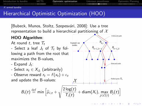
[Bubeck, Munos, Stoltz, Szepesvari, 2008]: Use a treerepresentation to build a hierarchical partitioning of XHOO Algorithm:At round t, tree Tt- Select a leaf Jt of Tt by fol-lowing a path from the root thatmaximizes the B-values,- Expand Jt :- Select xt ∈ XJt (arbitrarily)- Observe reward rt = f (xt) + ϵtand update the B-values:
h,iB
Bh+1,2i−1
Bh+1,2i
Xt
Turned−onnodes
Followed path
Selected node
Pulled point
Bi (t)def= min
[µi ,t +
√2 log(t)
Ti (t)+ diam(Xi ), max
j∈C(i)Bj(t)
]

. . . . . .
. . . . . . . . . . . . . . . . . . . . . . . . . . .Introduction to bandits
. . . . . .MCTS
. . . . . . . . . . . . . . . . . . . . . . . . . . . . . . . . . . .Optimistic optimization
. . . . . . . . . . . . . . . . . . . . . . . . . . . . . . .Unknown smoothness
. . . . . . . . . . . . . . . . . . .Optimistic Planning
X -armed bandits
Properties of HOO
HOO selects a leaf Jt such that
Jt ∈ argmaxj∈Lt
mini∈P(j)
[µi ,t +
√2 log(t)
Ti (t)+ diam(Xi )
]For any Xi ∋ x∗, Bi (t) is a h.p. UCB on f (x∗).
Thus any suboptimal node Xi such that
supx∈Xi
f (x) +
√2 log(t)
Ti (t)+ diam(Xi ) < f (x∗)
will not be selected.

. . . . . .
. . . . . . . . . . . . . . . . . . . . . . . . . . .Introduction to bandits
. . . . . .MCTS
. . . . . . . . . . . . . . . . . . . . . . . . . . . . . . . . . . .Optimistic optimization
. . . . . . . . . . . . . . . . . . . . . . . . . . . . . . .Unknown smoothness
. . . . . . . . . . . . . . . . . . .Optimistic Planning
X -armed bandits
Example in 1d
rt ∼ B(f (xt)) a Bernoulli distribution with parameter f (xt)
Resulting tree at time n = 1000 and at n = 10000.

. . . . . .
. . . . . . . . . . . . . . . . . . . . . . . . . . .Introduction to bandits
. . . . . .MCTS
. . . . . . . . . . . . . . . . . . . . . . . . . . . . . . . . . . .Optimistic optimization
. . . . . . . . . . . . . . . . . . . . . . . . . . . . . . .Unknown smoothness
. . . . . . . . . . . . . . . . . . .Optimistic Planning
X -armed bandits
Analysis of HOO
Assuming a slightly stronger assumption on f (weak Lipschitz):∀x , y ∈ X ,
f (y)− f (x) ≤ maxf ∗ − f (y), ℓ(x , y)
.Theorem 3...
......
Assume that the diameters decrease exponentially fast with theirdepth h. The loss of HOO is
rn = O([ n
log n
]− 1d+2
)(recall that for deterministic rewards rn = O(n−1/d) for d > 0)(see also the Zooming algorithm [Kleinberg, Slivkins, Upfal, 2008]).
. . . . . .
. . . . . . . . . . . . . . . . . . . . . . . . . . .Introduction to bandits
. . . . . .MCTS
. . . . . . . . . . . . . . . . . . . . . . . . . . . . . . . . . . .Optimistic optimization
. . . . . . . . . . . . . . . . . . . . . . . . . . . . . . .Unknown smoothness
. . . . . . . . . . . . . . . . . . .Optimistic Planning
X -armed bandits
Example
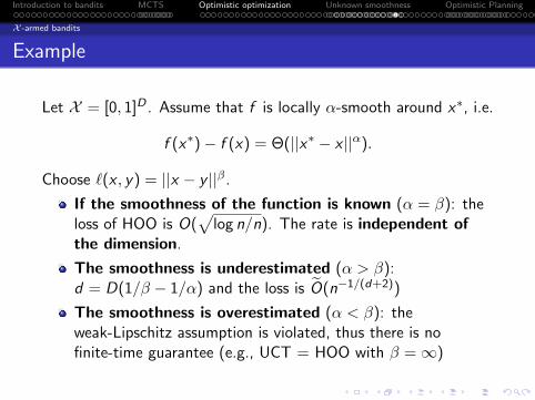
Let X = [0, 1]D . Assume that f is locally α-smooth around x∗, i.e.
f (x∗)− f (x) = Θ(||x∗ − x ||α).
Choose ℓ(x , y) = ||x − y ||β.If the smoothness of the function is known (α = β): theloss of HOO is O(
√log n/n). The rate is independent of
the dimension.
The smoothness is underestimated (α > β):d = D(1/β − 1/α) and the loss is O(n−1/(d+2))
The smoothness is overestimated (α < β): theweak-Lipschitz assumption is violated, thus there is nofinite-time guarantee (e.g., UCT = HOO with β = ∞)
. . . . . .
. . . . . . . . . . . . . . . . . . . . . . . . . . .Introduction to bandits
. . . . . .MCTS
. . . . . . . . . . . . . . . . . . . . . . . . . . . . . . . . . . .Optimistic optimization
. . . . . . . . . . . . . . . . . . . . . . . . . . . . . . .Unknown smoothness
. . . . . . . . . . . . . . . . . . .Optimistic Planning
X -armed bandits
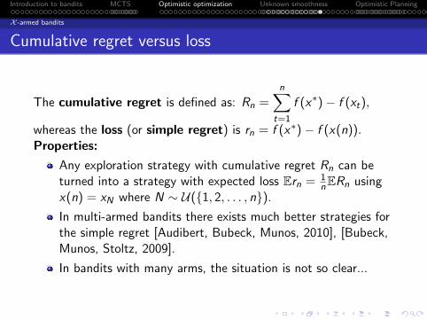
Cumulative regret versus loss
The cumulative regret is defined as: Rn =n∑
t=1
f (x∗)− f (xt),
whereas the loss (or simple regret) is rn = f (x∗)− f (x(n)).Properties:
Any exploration strategy with cumulative regret Rn can beturned into a strategy with expected loss Ern = 1
nERn usingx(n) = xN where N ∼ U(1, 2, . . . , n).In multi-armed bandits there exists much better strategies forthe simple regret [Audibert, Bubeck, Munos, 2010], [Bubeck,Munos, Stoltz, 2009].
In bandits with many arms, the situation is not so clear...

. . . . . .
. . . . . . . . . . . . . . . . . . . . . . . . . . .Introduction to bandits
. . . . . .MCTS
. . . . . . . . . . . . . . . . . . . . . . . . . . . . . . . . . . .Optimistic optimization
. . . . . . . . . . . . . . . . . . . . . . . . . . . . . . .Unknown smoothness
. . . . . . . . . . . . . . . . . . .Optimistic Planning
Assume that the smoothness is unknown
Previous algorithms heavily rely on the knowledge or the localsmoothness of the function (i.e. knowledge of the best metric).
Question: When the smoothness is unknown, is it possible toimplement the optimistic principle for function optimization?
Some approaches relies on estimating the local or globalsmoothness of the function [Bubeck, Stoltz, Yu, 2011], [Slivkins,2011], [Bull, 2013].
. . . . . .
. . . . . . . . . . . . . . . . . . . . . . . . . . .Introduction to bandits
. . . . . .MCTS
. . . . . . . . . . . . . . . . . . . . . . . . . . . . . . . . . . .Optimistic optimization
. . . . . . . . . . . . . . . . . . . . . . . . . . . . . . .Unknown smoothness
. . . . . . . . . . . . . . . . . . .Optimistic Planning
DIRECT algorithm
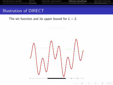
Assume f is Lipschitz but the Lipschitz constant L is unknown.
The DIRECT algorithm [Jones, Perttunen, Stuckman, 1993]expands simultaneously all nodes that may potentially contain themaximum for some value of L.
. . . . . .
. . . . . . . . . . . . . . . . . . . . . . . . . . .Introduction to bandits
. . . . . .MCTS
. . . . . . . . . . . . . . . . . . . . . . . . . . . . . . . . . . .Optimistic optimization
. . . . . . . . . . . . . . . . . . . . . . . . . . . . . . .Unknown smoothness
. . . . . . . . . . . . . . . . . . .Optimistic Planning
Illustration of DIRECT
The sin function and its upper bound for L = 2.

. . . . . .
. . . . . . . . . . . . . . . . . . . . . . . . . . .Introduction to bandits
. . . . . .MCTS
. . . . . . . . . . . . . . . . . . . . . . . . . . . . . . . . . . .Optimistic optimization
. . . . . . . . . . . . . . . . . . . . . . . . . . . . . . .Unknown smoothness
. . . . . . . . . . . . . . . . . . .Optimistic Planning
Illustration of DIRECT
The sin function and its upper bound for L = 1/2.
. . . . . .
. . . . . . . . . . . . . . . . . . . . . . . . . . .Introduction to bandits
. . . . . .MCTS
. . . . . . . . . . . . . . . . . . . . . . . . . . . . . . . . . . .Optimistic optimization
. . . . . . . . . . . . . . . . . . . . . . . . . . . . . . .Unknown smoothness
. . . . . . . . . . . . . . . . . . .Optimistic Planning
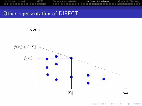
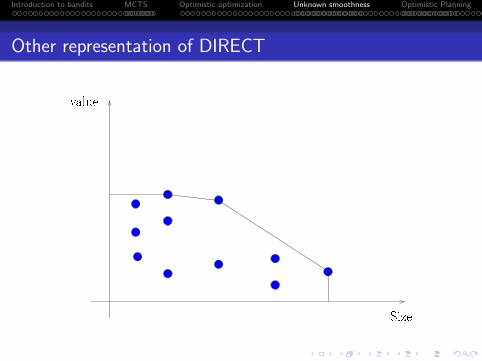
Other representation of DIRECT
Size|Xi|
f(xi) + L|Xi|
f(xi)
value
. . . . . .
. . . . . . . . . . . . . . . . . . . . . . . . . . .Introduction to bandits
. . . . . .MCTS
. . . . . . . . . . . . . . . . . . . . . . . . . . . . . . . . . . .Optimistic optimization
. . . . . . . . . . . . . . . . . . . . . . . . . . . . . . .Unknown smoothness
. . . . . . . . . . . . . . . . . . .Optimistic Planning
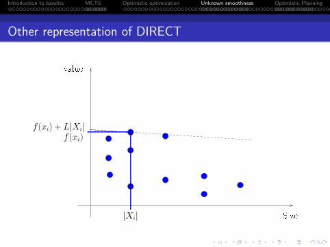
Other representation of DIRECT
Size
value
f(xi) + L|Xi|
|Xi|
f(xi)
. . . . . .
. . . . . . . . . . . . . . . . . . . . . . . . . . .Introduction to bandits
. . . . . .MCTS
. . . . . . . . . . . . . . . . . . . . . . . . . . . . . . . . . . .Optimistic optimization
. . . . . . . . . . . . . . . . . . . . . . . . . . . . . . .Unknown smoothness
. . . . . . . . . . . . . . . . . . .Optimistic Planning
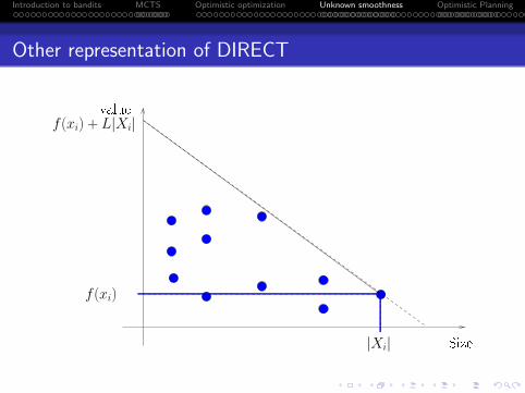
Other representation of DIRECT
Size
value
f(xi)
|Xi|
f(xi) + L|Xi|
. . . . . .
. . . . . . . . . . . . . . . . . . . . . . . . . . .Introduction to bandits
. . . . . .MCTS
. . . . . . . . . . . . . . . . . . . . . . . . . . . . . . . . . . .Optimistic optimization
. . . . . . . . . . . . . . . . . . . . . . . . . . . . . . .Unknown smoothness
. . . . . . . . . . . . . . . . . . .Optimistic Planning
Other representation of DIRECT
Size
value
. . . . . .
. . . . . . . . . . . . . . . . . . . . . . . . . . .Introduction to bandits
. . . . . .MCTS
. . . . . . . . . . . . . . . . . . . . . . . . . . . . . . . . . . .Optimistic optimization
. . . . . . . . . . . . . . . . . . . . . . . . . . . . . . .Unknown smoothness
. . . . . . . . . . . . . . . . . . .Optimistic Planning
Limitations of DIRECT
Assuming the function is globally Lipschitz is too restrictive. Wewould like to handle the general case where:
where the function is only locally smooth w.r.t. ℓ
for any semi-metric ℓ
. . . . . .
. . . . . . . . . . . . . . . . . . . . . . . . . . .Introduction to bandits
. . . . . .MCTS
. . . . . . . . . . . . . . . . . . . . . . . . . . . . . . . . . . .Optimistic optimization
. . . . . . . . . . . . . . . . . . . . . . . . . . . . . . .Unknown smoothness
. . . . . . . . . . . . . . . . . . .Optimistic Planning
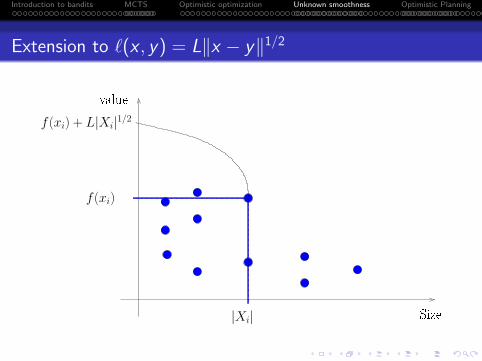
Extension to ℓ(x , y) = L∥x − y∥1/2
Size|Xi|
f(xi)
value
f(xi) + L|Xi|1/2

. . . . . .
. . . . . . . . . . . . . . . . . . . . . . . . . . .Introduction to bandits
. . . . . .MCTS
. . . . . . . . . . . . . . . . . . . . . . . . . . . . . . . . . . .Optimistic optimization
. . . . . . . . . . . . . . . . . . . . . . . . . . . . . . .Unknown smoothness
. . . . . . . . . . . . . . . . . . .Optimistic Planning
Extension to ℓ(x , y) = L∥x − y∥2
Size|Xi|
f(xi)
value
f(xi) + L|Xi|2

. . . . . .
. . . . . . . . . . . . . . . . . . . . . . . . . . .Introduction to bandits
. . . . . .MCTS
. . . . . . . . . . . . . . . . . . . . . . . . . . . . . . . . . . .Optimistic optimization
. . . . . . . . . . . . . . . . . . . . . . . . . . . . . . .Unknown smoothness
. . . . . . . . . . . . . . . . . . .Optimistic Planning
SOO
Extension to any ℓ!
Size
value

. . . . . .
. . . . . . . . . . . . . . . . . . . . . . . . . . .Introduction to bandits
. . . . . .MCTS
. . . . . . . . . . . . . . . . . . . . . . . . . . . . . . . . . . .Optimistic optimization
. . . . . . . . . . . . . . . . . . . . . . . . . . . . . . .Unknown smoothness
. . . . . . . . . . . . . . . . . . .Optimistic Planning
SOO
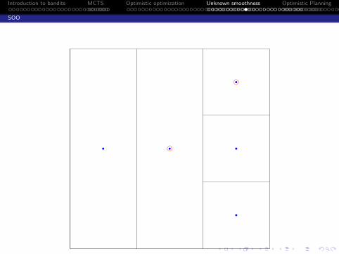
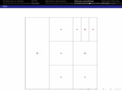
Simultaneous Optimistic Optimization (SOO)
[Munos, 2011]
Expand several leaves simultaneously
SOO expands at most one leaf per depth
SOO expands a leaf only if its value is larger that the value ofall leaves of same or lower depths.
At round t, SOO does not expand leaves with depth largerthan hmax(t)
. . . . . .
. . . . . . . . . . . . . . . . . . . . . . . . . . .Introduction to bandits
. . . . . .MCTS
. . . . . . . . . . . . . . . . . . . . . . . . . . . . . . . . . . .Optimistic optimization
. . . . . . . . . . . . . . . . . . . . . . . . . . . . . . .Unknown smoothness
. . . . . . . . . . . . . . . . . . .Optimistic Planning
SOO
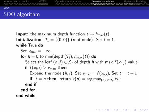
SOO algorithm
Input: the maximum depth function t 7→ hmax(t)Initialization: T1 = (0, 0) (root node). Set t = 1.while True doSet vmax = −∞.for h = 0 to min(depth(Tt), hmax(t)) do
Select the leaf (h, j) ∈ Lt of depth h with max f (xh,j) valueif f (xh,i ) > vmax then
Expand the node (h, i), Set vmax = f (xh,i ), Set t = t + 1if t = n then return x(n) = argmax(h,i)∈Tn xh,i
end ifend for
end while.

. . . . . .
. . . . . . . . . . . . . . . . . . . . . . . . . . .Introduction to bandits
. . . . . .MCTS
. . . . . . . . . . . . . . . . . . . . . . . . . . . . . . . . . . .Optimistic optimization
. . . . . . . . . . . . . . . . . . . . . . . . . . . . . . .Unknown smoothness
. . . . . . . . . . . . . . . . . . .Optimistic Planning
SOO
Performance of SOO
.Theorem 4...
......
For any semi-metric ℓ such that
f is locally smooth w.r.t. ℓ
The ℓ-diameter of cells of depth h is cγh
The near-optimality dimension of f w.r.t. ℓ is d = 0,
by choosing hmax(n) =√n, the expected loss of SOO is
rn ≤ cγ√n/C−1
In the case d > 0 a similar statement holds with Ern = O(n−1/d).

. . . . . .
. . . . . . . . . . . . . . . . . . . . . . . . . . .Introduction to bandits
. . . . . .MCTS
. . . . . . . . . . . . . . . . . . . . . . . . . . . . . . . . . . .Optimistic optimization
. . . . . . . . . . . . . . . . . . . . . . . . . . . . . . .Unknown smoothness
. . . . . . . . . . . . . . . . . . .Optimistic Planning
SOO
Performance of SOO
Remarks:
Since the algorithm does not depend on ℓ, the analysis holdsfor the best possible choice of the semi-metric ℓ satisfying theassumptions.
SOO does almost as well as DOO optimally fitted (thus“adapts” to the unknown local smoothness of f ).
. . . . . .
. . . . . . . . . . . . . . . . . . . . . . . . . . .Introduction to bandits
. . . . . .MCTS
. . . . . . . . . . . . . . . . . . . . . . . . . . . . . . . . . . .Optimistic optimization
. . . . . . . . . . . . . . . . . . . . . . . . . . . . . . .Unknown smoothness
. . . . . . . . . . . . . . . . . . .Optimistic Planning
SOO
Numerical experiments
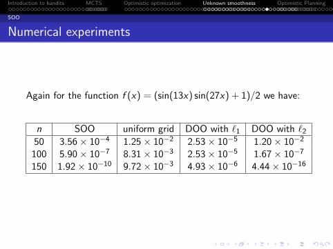
Again for the function f (x) = (sin(13x) sin(27x) + 1)/2 we have:
n SOO uniform grid DOO with ℓ1 DOO with ℓ250 3.56× 10⁻⁴ 1.25× 10⁻² 2.53× 10⁻⁵ 1.20× 10⁻²
100 5.90× 10⁻⁷ 8.31× 10⁻³ 2.53× 10⁻⁵ 1.67× 10⁻⁷
150 1.92× 10⁻¹⁰ 9.72× 10⁻³ 4.93× 10⁻⁶ 4.44× 10⁻¹⁶

. . . . . .
. . . . . . . . . . . . . . . . . . . . . . . . . . .Introduction to bandits
. . . . . .MCTS
. . . . . . . . . . . . . . . . . . . . . . . . . . . . . . . . . . .Optimistic optimization
. . . . . . . . . . . . . . . . . . . . . . . . . . . . . . .Unknown smoothness
. . . . . . . . . . . . . . . . . . .Optimistic Planning
SOO
The case d = 0 is non-trivial!
Example:
f is locally α-smooth around its maximum:
f (x∗)− f (x) = Θ(∥x∗ − x∥α),
for some α > 0.
SOO algorithm does not require the knowledge of ℓ,
Using ℓ(x , y) = ∥x − y∥α in the analysis, all assumptions aresatisfied (with γ = 3−α/D and d = 0, thus the loss of SOO isrn = O(3−
√nα/(CD)) (stretched-exponential loss),
This is almost as good as DOO optimally fitted!
(Extends to the case f (x∗)− f (x) ≈∑D
i=1 ci |x∗i − xi |αi )

. . . . . .
. . . . . . . . . . . . . . . . . . . . . . . . . . .Introduction to bandits
. . . . . .MCTS
. . . . . . . . . . . . . . . . . . . . . . . . . . . . . . . . . . .Optimistic optimization
. . . . . . . . . . . . . . . . . . . . . . . . . . . . . . .Unknown smoothness
. . . . . . . . . . . . . . . . . . .Optimistic Planning
SOO
The case d = 0
More generally, any function whose upper- and lower envelopesaround x∗ have the same shape: ∃c > 0 and η > 0, such that
min(η, cℓ(x , x∗)) ≤ f (x∗)− f (x) ≤ ℓ(x , x∗), for all x ∈ X .
has a near-optimality d = 0 (w.r.t. the metric ℓ).
x∗
f(x∗) f(x∗)− cℓ(x, x∗)
f(x∗)− ℓ(x, x∗)
f(x∗)− η
. . . . . .
. . . . . . . . . . . . . . . . . . . . . . . . . . .Introduction to bandits
. . . . . .MCTS
. . . . . . . . . . . . . . . . . . . . . . . . . . . . . . . . . . .Optimistic optimization
. . . . . . . . . . . . . . . . . . . . . . . . . . . . . . .Unknown smoothness
. . . . . . . . . . . . . . . . . . .Optimistic Planning
SOO
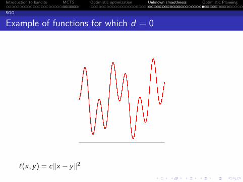
Example of functions for which d = 0
ℓ(x , y) = c∥x − y∥2

. . . . . .
. . . . . . . . . . . . . . . . . . . . . . . . . . .Introduction to bandits
. . . . . .MCTS
. . . . . . . . . . . . . . . . . . . . . . . . . . . . . . . . . . .Optimistic optimization
. . . . . . . . . . . . . . . . . . . . . . . . . . . . . . .Unknown smoothness
. . . . . . . . . . . . . . . . . . .Optimistic Planning
SOO
Example of functions with d = 0
ℓ(x , y) = c∥x − y∥1/2

. . . . . .
. . . . . . . . . . . . . . . . . . . . . . . . . . .Introduction to bandits
. . . . . .MCTS
. . . . . . . . . . . . . . . . . . . . . . . . . . . . . . . . . . .Optimistic optimization
. . . . . . . . . . . . . . . . . . . . . . . . . . . . . . .Unknown smoothness
. . . . . . . . . . . . . . . . . . .Optimistic Planning
SOO
d = 0?
ℓ(x , y) = c∥x − y∥1/2

. . . . . .
. . . . . . . . . . . . . . . . . . . . . . . . . . .Introduction to bandits
. . . . . .MCTS
. . . . . . . . . . . . . . . . . . . . . . . . . . . . . . . . . . .Optimistic optimization
. . . . . . . . . . . . . . . . . . . . . . . . . . . . . . .Unknown smoothness
. . . . . . . . . . . . . . . . . . .Optimistic Planning
SOO
d > 0
f (x) = 1−√x + (−x2 +
√x) ∗ (sin(1/x2) + 1)/2
The lower-envelope is of order 1/2 whereas the upper one is oforder 2. We deduce that d ≥ 3/2.

. . . . . .
. . . . . . . . . . . . . . . . . . . . . . . . . . .Introduction to bandits
. . . . . .MCTS
. . . . . . . . . . . . . . . . . . . . . . . . . . . . . . . . . . .Optimistic optimization
. . . . . . . . . . . . . . . . . . . . . . . . . . . . . . .Unknown smoothness
. . . . . . . . . . . . . . . . . . .Optimistic Planning
SOO
Sketch of proof
For any ℓ, defineIh = cells Xi of depth h such that f (xi ) + diam(h) ≥ f (x∗)Once the optimal cell of depth h has been expanded, it takesat most |Ih+1| cell expansions of depth h + 1 before theoptimal cell is expanded.
Thus n ≤ hmax(n)∑min(hmax(n),h∗n )
h=0 |Ih|, where h∗n is the depthof the node containing x∗.
Assuming d = 0, |Ih| ≤ C , and using hmax(n) =√n, we have√
n = C min(hmax(n), h∗n) = Ch∗n
Finally the value of the returned point x(n) is at least as goodas that of the optimal expanded node i∗n containing x∗:
f (x(n)) ≥ f (xi∗n ) ≥ f (x∗)− diam(h∗n) ≥ f (x∗)− cγ√n/C ,
where we used that the diameters are cγh.
. . . . . .
. . . . . . . . . . . . . . . . . . . . . . . . . . .Introduction to bandits
. . . . . .MCTS
. . . . . . . . . . . . . . . . . . . . . . . . . . . . . . . . . . .Optimistic optimization
. . . . . . . . . . . . . . . . . . . . . . . . . . . . . . .Unknown smoothness
. . . . . . . . . . . . . . . . . . .Optimistic Planning
SOO
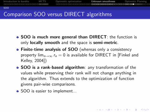
Comparison SOO versus DIRECT algorithms
SOO is much more general than DIRECT: the function isonly locally smooth and the space is semi-metric.
Finite-time analysis of SOO (whereas only a consistencyproperty limn→∞ rn = 0 is available for DIRECT in [Finkel andKelley, 2004])
SOO is a rank-based algorithm: any transformation of thevalues while preserving their rank will not change anything inthe algorithm. Thus extends to the optimization of functiongivens pair-wise comparisons.
SOO is easier to implement...

. . . . . .
. . . . . . . . . . . . . . . . . . . . . . . . . . .Introduction to bandits
. . . . . .MCTS
. . . . . . . . . . . . . . . . . . . . . . . . . . . . . . . . . . .Optimistic optimization
. . . . . . . . . . . . . . . . . . . . . . . . . . . . . . .Unknown smoothness
. . . . . . . . . . . . . . . . . . .Optimistic Planning
StoSOO
Stochastic SOO (StoSOO)
A simple way to extends SOO to the case of stochastic rewards isthe following:
Select a cell i (and sample f at xi ) according to SOO basedon the values
µi ,t + c
√log n
Tk(t),
(where µi ,t is the arerage rewards received at xi and Ti (t) isthe number of rewards received at state xi ),
Expand the cell Xi only if Ti (t) ≥ k, where k is a parameter.
Remark: This really looks like UCT, except that
several cells are selected at each round,
a cell is refined only when we received k samples.
. . . . . .
. . . . . . . . . . . . . . . . . . . . . . . . . . .Introduction to bandits
. . . . . .MCTS
. . . . . . . . . . . . . . . . . . . . . . . . . . . . . . . . . . .Optimistic optimization
. . . . . . . . . . . . . . . . . . . . . . . . . . . . . . .Unknown smoothness
. . . . . . . . . . . . . . . . . . .Optimistic Planning
StoSOO
Intuition for StoSOO
With high probability, StoSOO acts as a ϵ-pertubed version ofSOO where:
The values f (xi ) are perturbed by ϵ, where ϵ = O(√
log nk )
There are only m = n/k evaluations to the function.
Thus the loss of StoSOO is
Ern(StoSOO) = Erm(SOO) + O(
√log n
k)

. . . . . .
. . . . . . . . . . . . . . . . . . . . . . . . . . .Introduction to bandits
. . . . . .MCTS
. . . . . . . . . . . . . . . . . . . . . . . . . . . . . . . . . . .Optimistic optimization
. . . . . . . . . . . . . . . . . . . . . . . . . . . . . . .Unknown smoothness
. . . . . . . . . . . . . . . . . . .Optimistic Planning
StoSOO
Performance of StoSOO
.Theorem 5 (Valko, Carpentier, Munos, 2013)...
......
For any semi-metric ℓ such that
f is locally smooth w.r.t. ℓ
The ℓ-diameters of the cells decrease exponentially fast withtheir depth,
The near-optimality dimension of f w.r.t. ℓ is d = 0,
by choosing k = n(log n)3
, hmax(n) = (log n)3/2, the expected loss of
StoSOO is
Ern = O((log n)2√
n
).

. . . . . .
. . . . . . . . . . . . . . . . . . . . . . . . . . .Introduction to bandits
. . . . . .MCTS
. . . . . . . . . . . . . . . . . . . . . . . . . . . . . . . . . . .Optimistic optimization
. . . . . . . . . . . . . . . . . . . . . . . . . . . . . . .Unknown smoothness
. . . . . . . . . . . . . . . . . . .Optimistic Planning
StoSOO
Comments about StoSOO
In the (rather general) case d = 0, StoSOO gives a O(1/√n) loss
In comparison to HOO/Zooming:
HOO optimally fitted gives O(√
log nn
)loss
HOO with underestimation of the right smoothnessdeteriorates
HOO with overestimation of the right smoothness may notconverge.
Thus StoSOO is almost as good as HOO optimally fitted.

. . . . . .
. . . . . . . . . . . . . . . . . . . . . . . . . . .Introduction to bandits
. . . . . .MCTS
. . . . . . . . . . . . . . . . . . . . . . . . . . . . . . . . . . .Optimistic optimization
. . . . . . . . . . . . . . . . . . . . . . . . . . . . . . .Unknown smoothness
. . . . . . . . . . . . . . . . . . .Optimistic Planning
StoSOO
Range of application of DOO/HOO and SOO/StoSOO
Illustrations in Euclidean spaces [0, 1]D only.
But there are plenty of other semi-metric spaces:
Trees, graphs, combinatorial spaces, structured spaces, ...
Ex: space of policies for MDPs
We only require:
the search space X to be equipped with a semi-metric ℓ
a nested (hierarchical) partitioning of the space, such that theℓ-diameters of the cells decrease with their depth
f to satisfy a local smoothness property w.r.t. ℓ
ℓ may or may not be known.

. . . . . .
. . . . . . . . . . . . . . . . . . . . . . . . . . .Introduction to bandits
. . . . . .MCTS
. . . . . . . . . . . . . . . . . . . . . . . . . . . . . . . . . . .Optimistic optimization
. . . . . . . . . . . . . . . . . . . . . . . . . . . . . . .Unknown smoothness
. . . . . . . . . . . . . . . . . . .Optimistic Planning
Online planning in a MDP
Setting:
Assume we have a model of the MDP.
The state space is large: no way to approximate the valuefunction
Search for the best policy given an initial state, using a finitenumerical budget (number of calls to the model)
Protocol:
From current state sk , perform planning using n calls to themodel and recommend action a(n),
Play a(n), observe next state sk+1, and repeat
Loss: rndef= max
a∈AQ∗(sk , a)− Q∗(sk , a(n)).

. . . . . .
. . . . . . . . . . . . . . . . . . . . . . . . . . .Introduction to bandits
. . . . . .MCTS
. . . . . . . . . . . . . . . . . . . . . . . . . . . . . . . . . . .Optimistic optimization
. . . . . . . . . . . . . . . . . . . . . . . . . . . . . . .Unknown smoothness
. . . . . . . . . . . . . . . . . . .Optimistic Planning
Deterministic dynamics
Deterministic transitions and rewards
(infinite time horizon and discounted setting)
A policy x is an infinite path
Value f (x) =∑
s≥0 γsrs(x), where
the rewards are in [0, 1]
Metric: ℓ(x , y) = γh(x,y)
1−γ
Prop: f (x) is Lipschitz w.r.t. ℓ
→ Use optimistic search
Initial state
xy
h(x, y) = 2

. . . . . .
. . . . . . . . . . . . . . . . . . . . . . . . . . .Introduction to bandits
. . . . . .MCTS
. . . . . . . . . . . . . . . . . . . . . . . . . . . . . . . . . . .Optimistic optimization
. . . . . . . . . . . . . . . . . . . . . . . . . . . . . . .Unknown smoothness
. . . . . . . . . . . . . . . . . . .Optimistic Planning
Deterministic dynamics
OPD algorithm
Optimistic Planning in Deterministic systems:
Define the B-values:
Bidef=
d(i)∑s=0
γsrs +γd(i)+1
1− γ
We have Bi ≥ maxx∋i f (x)
For each round t = 1 to n,expand the node withhighest B-value
Observe reward, updateB-values
Optimal path
Expandednodes
Node i
Recommend the first action a(n) of the best policy.

. . . . . .
. . . . . . . . . . . . . . . . . . . . . . . . . . .Introduction to bandits
. . . . . .MCTS
. . . . . . . . . . . . . . . . . . . . . . . . . . . . . . . . . . .Optimistic optimization
. . . . . . . . . . . . . . . . . . . . . . . . . . . . . . .Unknown smoothness
. . . . . . . . . . . . . . . . . . .Optimistic Planning
Deterministic dynamics
Performance of OPD
Define β such that P(Random path is ϵ-optimal) = O(ϵβ).
Define κdef= Kγβ ∈ [1,K ]. Then κ is the branching factor of the
set of near-optimal sequences:
I =sequences of length h such that
h∑s=0
γs rs ≥ V ∗ − γh+1
1− γ
.
Property: κ relates to the near-opt. dimension d = log κlog 1/γ (the set
of ϵ-optimal paths is covered by O(ϵ−d) ℓ-balls of radius ϵ)
Loss of OPD [Hren and Munos, 2008]:
rn = O(n−1d ) = O
(n−
log 1/γlog κ
).
Performance depends on the quantity of near-optimal policies
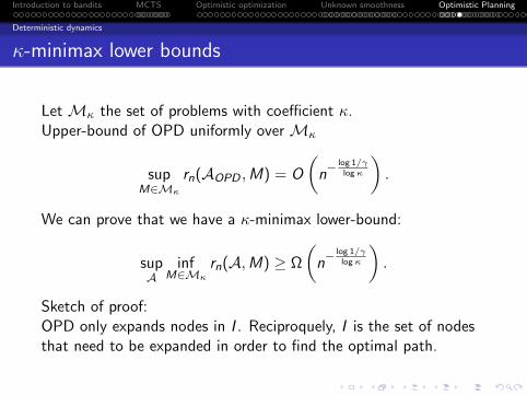
. . . . . .
. . . . . . . . . . . . . . . . . . . . . . . . . . .Introduction to bandits
. . . . . .MCTS
. . . . . . . . . . . . . . . . . . . . . . . . . . . . . . . . . . .Optimistic optimization
. . . . . . . . . . . . . . . . . . . . . . . . . . . . . . .Unknown smoothness
. . . . . . . . . . . . . . . . . . .Optimistic Planning
Deterministic dynamics
κ-minimax lower bounds
Let Mκ the set of problems with coefficient κ.Upper-bound of OPD uniformly over Mκ
supM∈Mκ
rn(AOPD ,M) = O
(n−
log 1/γlog κ
).
We can prove that we have a κ-minimax lower-bound:
supA
infM∈Mκ
rn(A,M) ≥ Ω
(n−
log 1/γlog κ
).
Sketch of proof:OPD only expands nodes in I . Reciproquely, I is the set of nodesthat need to be expanded in order to find the optimal path.
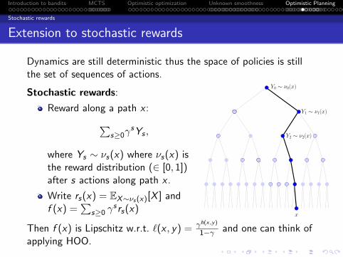
. . . . . .
. . . . . . . . . . . . . . . . . . . . . . . . . . .Introduction to bandits
. . . . . .MCTS
. . . . . . . . . . . . . . . . . . . . . . . . . . . . . . . . . . .Optimistic optimization
. . . . . . . . . . . . . . . . . . . . . . . . . . . . . . .Unknown smoothness
. . . . . . . . . . . . . . . . . . .Optimistic Planning
Stochastic rewards
Extension to stochastic rewards
Dynamics are still deterministic thus the space of policies is stillthe set of sequences of actions.
Stochastic rewards:
Reward along a path x :∑s≥0γ
sYs ,
where Ys ∼ νs(x) where νs(x) isthe reward distribution (∈ [0, 1])after s actions along path x .
Write rs(x) = EX∼νs(x)[X ] andf (x) =
∑s≥0 γ
srs(x)x
Y2 ∼ ν2(x)
Y1 ∼ ν1(x)
Y0 ∼ ν0(x)
Then f (x) is Lipschitz w.r.t. ℓ(x , y) = γh(x,y)
1−γ and one can think ofapplying HOO.
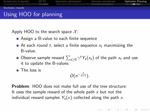
. . . . . .
. . . . . . . . . . . . . . . . . . . . . . . . . . .Introduction to bandits
. . . . . .MCTS
. . . . . . . . . . . . . . . . . . . . . . . . . . . . . . . . . . .Optimistic optimization
. . . . . . . . . . . . . . . . . . . . . . . . . . . . . . .Unknown smoothness
. . . . . . . . . . . . . . . . . . .Optimistic Planning
Stochastic rewards
Using HOO for planning
Apply HOO to the search space X :
Assign a B-value to each finite sequence
At each round t, select a finite sequence xt maximizing theB-value.
Observe sample reward∑
s≥0 γsYs(xt) of the path xt and use
it to update the B-values.
The loss isO(n−
1d+2 ).
Problem: HOO does not make full use of the tree structure:It uses the sample reward of the whole path x but not theindividual reward samples Ys(x) collected along the path x .

. . . . . .
. . . . . . . . . . . . . . . . . . . . . . . . . . .Introduction to bandits
. . . . . .MCTS
. . . . . . . . . . . . . . . . . . . . . . . . . . . . . . . . . . .Optimistic optimization
. . . . . . . . . . . . . . . . . . . . . . . . . . . . . . .Unknown smoothness
. . . . . . . . . . . . . . . . . . .Optimistic Planning
Stochastic rewards
Optimistic sampling using the tree structure
Open Loop Optimistic Planning (OLOP) [Bubeck, Munos,2010]:
At round t, play path xt (up to depth h = 12
log nlog 1/γ )
Observe sample rewards Ys(xt) of each node along the path xt
Compute empirical rewards µt(x1:s) for each node x1:s ofdepth s ≤ h
Define bound for each path x :
Bt(x) = min1≤j≤h
[ j∑s=0
γs(µt(x1:s) +
√2 log n
Tx1:s (t)
)+
γj+1
1− γ
]Select path xt+1 = argmaxx Bt(x)
This algorithm fully uses the tree structure of the rewards.

. . . . . .
. . . . . . . . . . . . . . . . . . . . . . . . . . .Introduction to bandits
. . . . . .MCTS
. . . . . . . . . . . . . . . . . . . . . . . . . . . . . . . . . . .Optimistic optimization
. . . . . . . . . . . . . . . . . . . . . . . . . . . . . . .Unknown smoothness
. . . . . . . . . . . . . . . . . . .Optimistic Planning
Stochastic rewards
Performance of OLOP
Define
β ≥ 0 such that P(Random path is ϵ-optimal) = O(ϵβ).
or κdef= Kγβ ∈ [1,K ] the branching factor of the set of
near-optimal sequences.
or the near-optimality dimension, d = log κlog 1/γ .
.Theorem 6 (Loss of OLOP)...
......
After n calls to the generative model,
Ern = f (x∗)− Ef (x(n)) =
O(n−1/d
)if d ≥ 2
O(1/
√n)
if d < 2
Much better than HOO! As good as OPD for d ≥ 2.
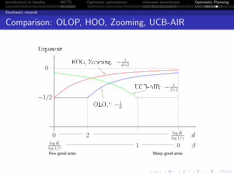
. . . . . .
. . . . . . . . . . . . . . . . . . . . . . . . . . .Introduction to bandits
. . . . . .MCTS
. . . . . . . . . . . . . . . . . . . . . . . . . . . . . . . . . . .Optimistic optimization
. . . . . . . . . . . . . . . . . . . . . . . . . . . . . . .Unknown smoothness
. . . . . . . . . . . . . . . . . . .Optimistic Planning
Stochastic rewards
Comparison: OLOP, HOO, Zooming, UCB-AIR
Many good armsFew good arms
logKlog 1/γ
logKlog 1/γ
d
β
0 2
1 0
Exponent
0HOO, Zooming:
OLOP:
UCB-AIR:
−
1d+2
−
1d
−
1β+1
−1/2
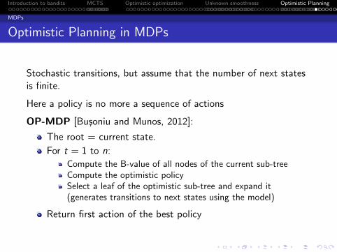
. . . . . .
. . . . . . . . . . . . . . . . . . . . . . . . . . .Introduction to bandits
. . . . . .MCTS
. . . . . . . . . . . . . . . . . . . . . . . . . . . . . . . . . . .Optimistic optimization
. . . . . . . . . . . . . . . . . . . . . . . . . . . . . . .Unknown smoothness
. . . . . . . . . . . . . . . . . . .Optimistic Planning
MDPs
Optimistic Planning in MDPs
Stochastic transitions, but assume that the number of next statesis finite.
Here a policy is no more a sequence of actions
OP-MDP [Busoniu and Munos, 2012]:
The root = current state.
For t = 1 to n:
Compute the B-value of all nodes of the current sub-treeCompute the optimistic policySelect a leaf of the optimistic sub-tree and expand it(generates transitions to next states using the model)
Return first action of the best policy

. . . . . .
. . . . . . . . . . . . . . . . . . . . . . . . . . .Introduction to bandits
. . . . . .MCTS
. . . . . . . . . . . . . . . . . . . . . . . . . . . . . . . . . . .Optimistic optimization
. . . . . . . . . . . . . . . . . . . . . . . . . . . . . . .Unknown smoothness
. . . . . . . . . . . . . . . . . . .Optimistic Planning
MDPs
Illustration of OP-MDP
B-values: upper-bounds on the optimal value function V ∗(s):
B(s) =1
1− γfor leaves
B(s) = maxa
∑s′
p(s ′|s, a)[r(s, a, s ′) + γB(s ′)
]Compute the optimistic policy π+.

. . . . . .
. . . . . . . . . . . . . . . . . . . . . . . . . . .Introduction to bandits
. . . . . .MCTS
. . . . . . . . . . . . . . . . . . . . . . . . . . . . . . . . . . .Optimistic optimization
. . . . . . . . . . . . . . . . . . . . . . . . . . . . . . .Unknown smoothness
. . . . . . . . . . . . . . . . . . .Optimistic Planning
MDPs
Optimistic Planning in MDPs
Expand leaf in π+ with largest contribution: argmaxs∈L P(s)γd(s)
1−γ ,
where P(s) is the probability to reach s when following π+.
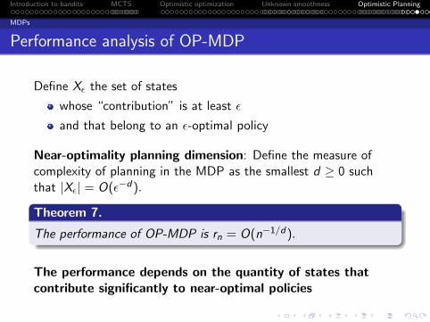
. . . . . .
. . . . . . . . . . . . . . . . . . . . . . . . . . .Introduction to bandits
. . . . . .MCTS
. . . . . . . . . . . . . . . . . . . . . . . . . . . . . . . . . . .Optimistic optimization
. . . . . . . . . . . . . . . . . . . . . . . . . . . . . . .Unknown smoothness
. . . . . . . . . . . . . . . . . . .Optimistic Planning
MDPs
Performance analysis of OP-MDP
Define Xϵ the set of states
whose “contribution” is at least ϵ
and that belong to an ϵ-optimal policy
Near-optimality planning dimension: Define the measure ofcomplexity of planning in the MDP as the smallest d ≥ 0 suchthat |Xϵ| = O(ϵ−d)..Theorem 7...
......The performance of OP-MDP is rn = O(n−1/d).
The performance depends on the quantity of states thatcontribute significantly to near-optimal policies

. . . . . .
. . . . . . . . . . . . . . . . . . . . . . . . . . .Introduction to bandits
. . . . . .MCTS
. . . . . . . . . . . . . . . . . . . . . . . . . . . . . . . . . . .Optimistic optimization
. . . . . . . . . . . . . . . . . . . . . . . . . . . . . . .Unknown smoothness
. . . . . . . . . . . . . . . . . . .Optimistic Planning
MDPs
Illustration of the performance
Reminder: rn = O(n−1/d).
Uniform rewards and probabilities d = logK+logNlog 1/γ (uniform
planning)
Structured rewards, uniform probabilities d = logNlog 1/γ (uniform
planning for a single policy)
Uniform rewards, concentrated probabilities d → logKlog 1/γ
(planning in deterministic systems)
Structured rewards, concentrated probabilities d → 0(exponential rate)
Remarks: d is small when
Structured rewards
Heterogeneous transition probabilities

. . . . . .
. . . . . . . . . . . . . . . . . . . . . . . . . . .Introduction to bandits
. . . . . .MCTS
. . . . . . . . . . . . . . . . . . . . . . . . . . . . . . . . . . .Optimistic optimization
. . . . . . . . . . . . . . . . . . . . . . . . . . . . . . .Unknown smoothness
. . . . . . . . . . . . . . . . . . .Optimistic Planning
MDPs
Towards d-minimax lower bounds
Let Md the set of MDPs with near-optimality planning dim. dUpper-bound of OP-MDP uniformly over Mβ
supM∈Md
rn(AOP−MDP ,M) ≤ O(n−1/d).
We conjecture that we have a d-minimax lower-bound:
supA
infM∈Md
Ern(A,M) ≥ Ω(n−1/d).

. . . . . .
. . . . . . . . . . . . . . . . . . . . . . . . . . .Introduction to bandits
. . . . . .MCTS
. . . . . . . . . . . . . . . . . . . . . . . . . . . . . . . . . . .Optimistic optimization
. . . . . . . . . . . . . . . . . . . . . . . . . . . . . . .Unknown smoothness
. . . . . . . . . . . . . . . . . . .Optimistic Planning
MDPs
Conclusions on optimistic planning
Perform optimistic search in policy space.
In deterministic dynamics, deterministic rewards, can be seenas a direct application of optimistic optimization
In stochastic rewards, the structure of the reward function canhelp estimation of paths given samples from other paths
In MDPs the near-optimality planning dimension is a newmeasure of the quantity of states that need to be expanded(the set of states that significantly contribute to near-optimalpolicies)
Fast rates when the MDP has structured rewards andheterogeneous transition probabilities.
Applications to Bayesian Reinforcement learning and planningin POMDPs.

. . . . . .
. . . . . . . . . . . . . . . . . . . . . . . . . . .Introduction to bandits
. . . . . .MCTS
. . . . . . . . . . . . . . . . . . . . . . . . . . . . . . . . . . .Optimistic optimization
. . . . . . . . . . . . . . . . . . . . . . . . . . . . . . .Unknown smoothness
. . . . . . . . . . . . . . . . . . .Optimistic Planning
MDPs
Possible extensions in optimistic planning
Extends OP-MDP to the case when only a generative modelof the dynamics is available
Extension to a possibly infinite number of next-states
Apply SOO / StoSOO ideas for planning: Although the value
function is Lipschitz w.r.t. the metric ℓ(x , y) = γh(x,y
1−γ , it maypossess additional smoothness around the maximum with ahigher-order semi-metric.
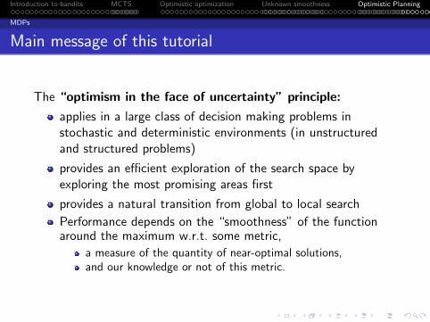
. . . . . .
. . . . . . . . . . . . . . . . . . . . . . . . . . .Introduction to bandits
. . . . . .MCTS
. . . . . . . . . . . . . . . . . . . . . . . . . . . . . . . . . . .Optimistic optimization
. . . . . . . . . . . . . . . . . . . . . . . . . . . . . . .Unknown smoothness
. . . . . . . . . . . . . . . . . . .Optimistic Planning
MDPs
Main message of this tutorial
The “optimism in the face of uncertainty” principle:
applies in a large class of decision making problems instochastic and deterministic environments (in unstructuredand structured problems)
provides an efficient exploration of the search space byexploring the most promising areas first
provides a natural transition from global to local search
Performance depends on the “smoothness” of the functionaround the maximum w.r.t. some metric,
a measure of the quantity of near-optimal solutions,and our knowledge or not of this metric.

. . . . . .
. . . . . . . . . . . . . . . . . . . . . . . . . . .Introduction to bandits
. . . . . .MCTS
. . . . . . . . . . . . . . . . . . . . . . . . . . . . . . . . . . .Optimistic optimization
. . . . . . . . . . . . . . . . . . . . . . . . . . . . . . .Unknown smoothness
. . . . . . . . . . . . . . . . . . .Optimistic Planning
MDPs
Conclusions
Thanks !!!
Slides and a review paper are available from my web page:
http://chercheurs.lille.inria.fr/∼munos/