Friction Flow in a PipeFriction Flow in a Pipe

Friction flow in a Pipe Finite Element TutorialFriction flow in a Pipe Finite Element Tutorial By Dr. Essam A. Ibrahim, Tuskegee University, Mechanical By Dr. Essam A. Ibrahim, Tuskegee University, Mechanical

Engineering Dept., Engineering Dept., emeei@tuskegee.eduemeei@tuskegee.edu Copyright 2006 Copyright 2006 Expected completion time for this tutorial: 45 minutes to 1 hourExpected completion time for this tutorial: 45 minutes to 1 hour Companion tutorial for Fluid Mechanics CourseCompanion tutorial for Fluid Mechanics Course Reference text: Fluid Mechanics, 5Reference text: Fluid Mechanics, 5thth Edition by Frank M. White Edition by Frank M. White

Table of ContentsTable of Contents

Educational Objectives Problem Description Creating the parts Assembly of the parts Solving with FloWorks Viewing the Results of the FE Analysis Comparison of Analytical to Finite Element Ana

lysis Conclusion Acknowledgment

Educational ObjectivesEducational Objectives

1. Be familiar with the basis of FE theory for three-dimensional flow analysis.

2. Understand the fundamentals of internal flow through the use of the COSMOS FloWorks finite element software.

3. Be able to construct a correct solid model using the SolidWorks CAD and perform an accurate finite element analysis using COSMOS FloWorks.

4. Learn to apply the appropriate ambient and boundary conditions and decide on the suitable size for the computational domain.

5. Know how to interpret and evaluate finite element solution quality including the process of validating the solution using the Moody Chart.

Problem Description 1Problem Description 1 Case:Case:

Ten liters per second of water at 25Ten liters per second of water at 25CC is to flow through a horizontal is to flow through a horizontal pipe 10 m long. We need to estimate the pressure drop in a cast pipe 10 m long. We need to estimate the pressure drop in a cast iron pipe of circular cross section of 10 cm diameter.iron pipe of circular cross section of 10 cm diameter.

Methods:Methods:

We use SolidWorks to design the model; COSMOS FloWorks to We use SolidWorks to design the model; COSMOS FloWorks to determine the pressure drop in the turbulent pipe flow with non-zero determine the pressure drop in the turbulent pipe flow with non-zero inner surface roughness. inner surface roughness.

Validation:Validation:Once the CFD solution is obtained, the results are to be compared Once the CFD solution is obtained, the results are to be compared with the analytic solutions using the Moody Chart. with the analytic solutions using the Moody Chart.

Problem Description 2Problem Description 2

A cast iron pipe with rough inner surfaceA cast iron pipe with rough inner surface

Volumetric Flow Rate,

Q= 10 liters/sec

Water Temperature,

T= 25C

Ambient Pressure,

P= 1.0 ATM

Inner diameter = 10 cm

Outer diameter = 12 cm

Inlet

Exit

Pipe Length,L= 10 meters

P1

P2

Pressure Drop,Pressure Drop,

PP2 2 - P- P11 = ? = ?

Steps to AnalysisSteps to Analysis

1.1. Modeling of the system with SolidWorks Modeling of the system with SolidWorks CAD suitesCAD suites

2.2. Meshing and solving the flow with Meshing and solving the flow with COSOMOS FloWorks CFD solver suitesCOSOMOS FloWorks CFD solver suites

3.3. Calculating the analytic solution and Calculating the analytic solution and validating the CFD resultsvalidating the CFD results

Modeling with SolidWorksModeling with SolidWorks

Create a new SolidWorks working window by choosing ‘a Create a new SolidWorks working window by choosing ‘a

3D representaion of a single design component’ option3D representaion of a single design component’ option

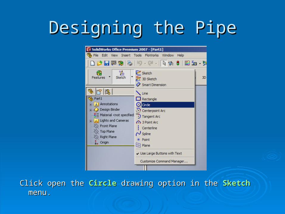
Designing the PipeDesigning the Pipe

Click open the Click open the CircleCircle drawing option in the drawing option in the SketchSketch menu. menu.

11Enter Sketch mode

x, y, z = (0, 0, 0)

50 mm

60 mm

Creating the cross section of the pipe 1Creating the cross section of the pipe 1

22 Create concentric circles for the inner and outer surfaces of the pipe

x, y, z = (0, 0, 0)

50 mm

60 mm

Creating the cross section of the pipe 2Creating the cross section of the pipe 2

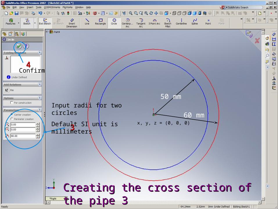
33

Input radii for two circles

Default SI unit is millimetersx, y, z = (0, 0, 0)

50 mm

60 mm

44 Confirm

Creating the cross section of the pipe 3Creating the cross section of the pipe 3

11Click FeaturesFeatures, choose ExtrudeExtrude

Use these buttons to change the view, e.g., zoom in and out, move, and pan.

Extruding circles to form a 3-D pipe 1Extruding circles to form a 3-D pipe 1

33

22

Confirm

Enter the length of the pipe.When 10.0 m is entered, it will show 100000.00mm since the default SI unit is set in millimeters.

Extruding circles to form a 3-D pipe 2Extruding circles to form a 3-D pipe 2

Creating Inlet and Exit lidsCreating Inlet and Exit lids

Once pipe is created and saved with a file extension of *.SLDPRT, Once pipe is created and saved with a file extension of *.SLDPRT, then inlet and exit lids are to be modeled in new working windows.then inlet and exit lids are to be modeled in new working windows.

These imaginary lids are needed to impose both Initial and These imaginary lids are needed to impose both Initial and Boundary Conditions for the COSMOS FloWorks to solve the flow. Boundary Conditions for the COSMOS FloWorks to solve the flow.

The Inlet and Exit lid modeling procedure is identical to that of the The Inlet and Exit lid modeling procedure is identical to that of the pipe modeling. The pipe modeling. The CircleCircle and and ExtrudeExtrude radio buttons are used to radio buttons are used to enable the modes.enable the modes.

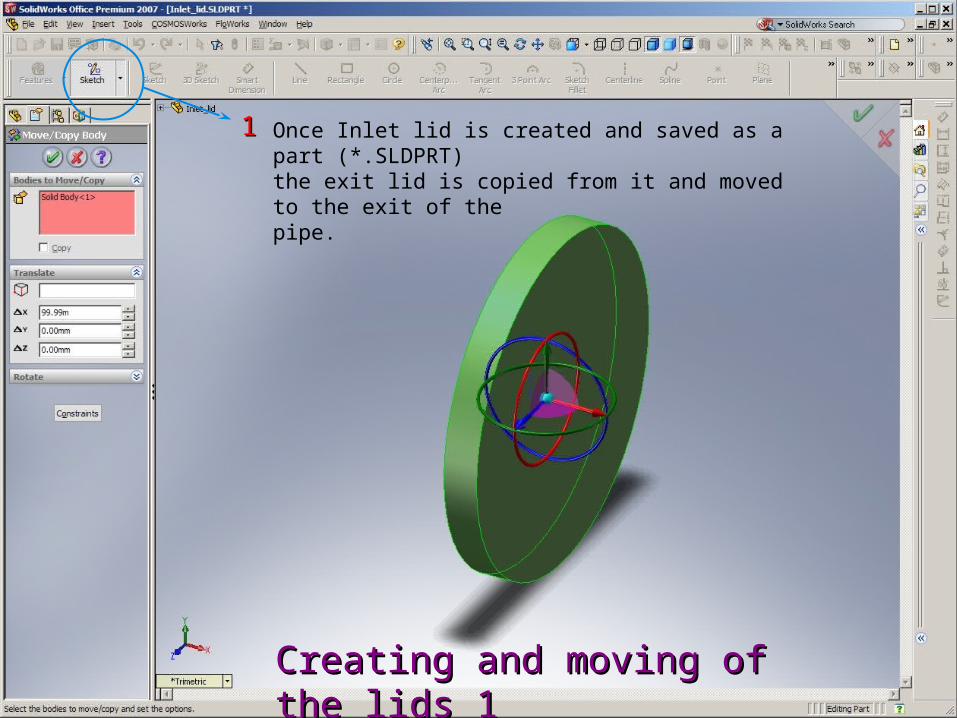
11 Once Inlet lid is created and saved as a part (*.SLDPRT)the exit lid is copied from it and moved to the exit of the pipe.

Creating and moving of the lids 1Creating and moving of the lids 1

22Select along which axis the body is to be moved.

Creating and moving of the lids 2Creating and moving of the lids 2

33

44 Confirm and save

Move/Copy of the Body function is selected fromInsert – Features –Move/Copy menu buttons.

Enter the distance the body has to translate.

Creating and moving of the lids 3Creating and moving of the lids 3

Assembly of the partsAssembly of the parts

So far three parts are modeled and saved separately: Pipe, Inlet So far three parts are modeled and saved separately: Pipe, Inlet lid, and Exit lid.lid, and Exit lid.

Next step is to assemble parts to form a complete working model Next step is to assemble parts to form a complete working model which will be used to in COSMOS FloWorks CFD Suite.which will be used to in COSMOS FloWorks CFD Suite.

Assembly of the parts are done using the Assembly of the parts are done using the Insert – PartInsert – Part menu. menu.

First open any part file and then insert parts one by one in one First open any part file and then insert parts one by one in one working window.working window.

Inserting ComponentsInserting Components Assembly of the parts can be performed by using Insert Component menu.

Selecting the biggest object first is recommended. Subsequently select all the remaining parts to the model that is being assembled.

It is very critical to verify that each part is inserted intended location.

Even If there is (are) mismatch(es) of the parts, it still can be saved as a whole assembly. This will cause errors in the COSMOS FloWorks later on.

11

Select Part sub menu in the Insert Function. Then select which part is to be inserted.

Assembly of the parts 1Assembly of the parts 1

22

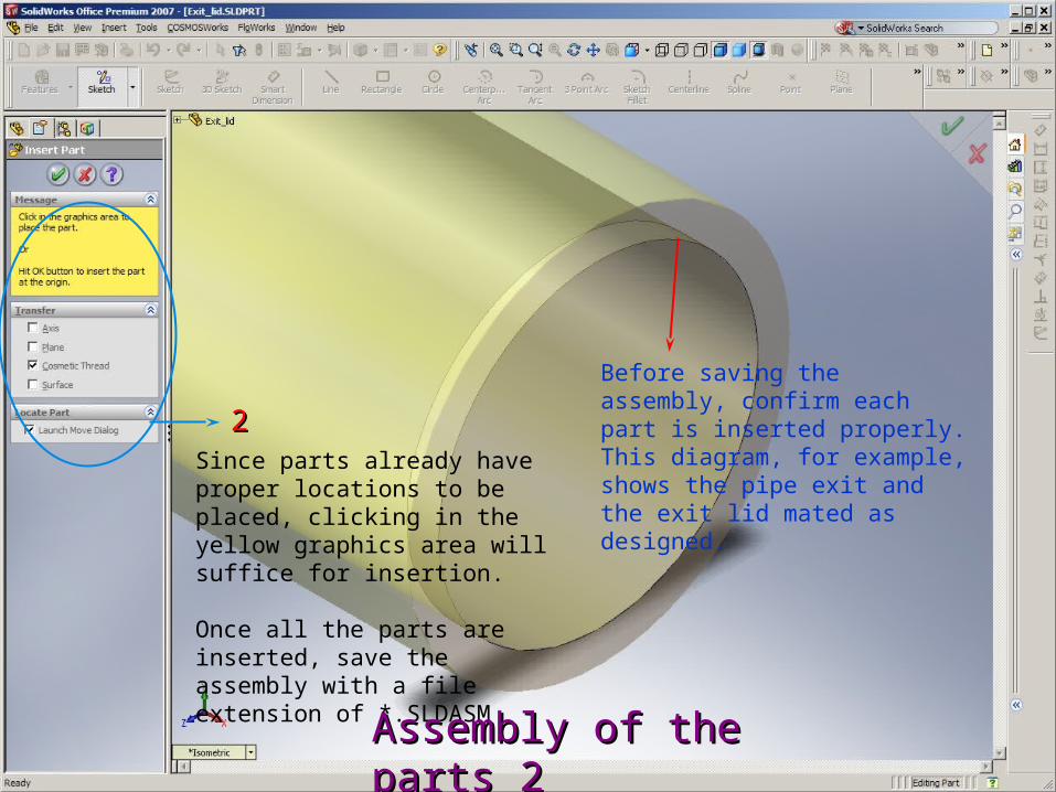
Before saving the assembly, confirm each part is inserted properly. This diagram, for example, shows the pipe exit and the exit lid mated as designed.

Since parts already have proper locations to be placed, clicking in the yellow graphics area will suffice for insertion.

Once all the parts are inserted, save the assembly with a file extension of *.SLDASM

Assembly of the parts 2Assembly of the parts 2

Solving with FloWorksSolving with FloWorks

Once the model is designed and assembled, the turbulent pipe flow Once the model is designed and assembled, the turbulent pipe flow can be solved using the COSMOS FloWorks CFD Solver suite.can be solved using the COSMOS FloWorks CFD Solver suite.

Proper assigning of the solid and liquid properties is as important as Proper assigning of the solid and liquid properties is as important as accurate inputting of Initial and Boundary conditions.accurate inputting of Initial and Boundary conditions.

Solver sequence is as follows:Solver sequence is as follows:

Project Configuration – Units – Computational Domain- Initial & Project Configuration – Units – Computational Domain- Initial & Boundary Conditions – Solve - AnalysesBoundary Conditions – Solve - Analyses

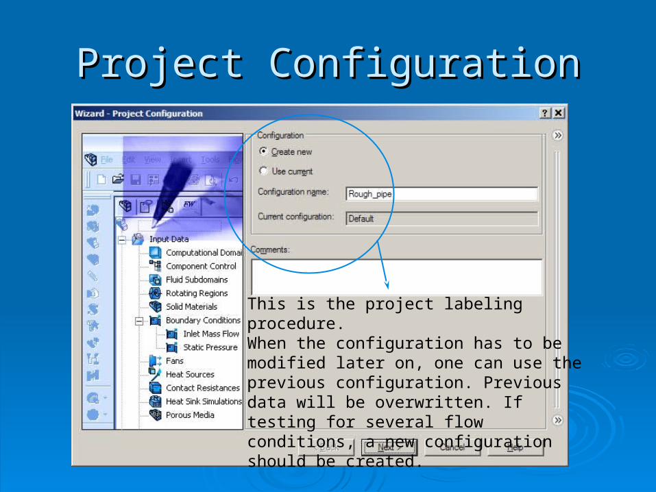
Project ConfigurationProject Configuration

This is the project labeling procedure.When the configuration has to be modified later on, one can use the previous configuration. Previous data will be overwritten. If testing for several flow conditions, a new configuration should be created.

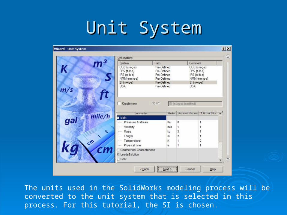
Unit SystemUnit System

The units used in the SolidWorks modeling process will be converted to the unit system that is selected in this process. For this tutorial, the SI is chosen.

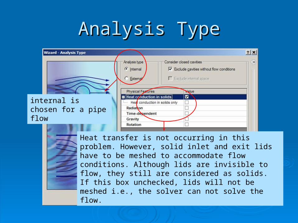
Analysis TypeAnalysis Type

internal is chosen for a pipe flow

Heat transfer is not occurring in this problem. However, solid inlet and exit lids have to be meshed to accommodate flow conditions. Although lids are invisible to flow, they still are considered as solids. If this box unchecked, lids will not be meshed i.e., the solver can not solve the flow.

Fluid PropertyFluid Property

Select Water for the working fluid

This flow has both Laminar and Turbulent region.

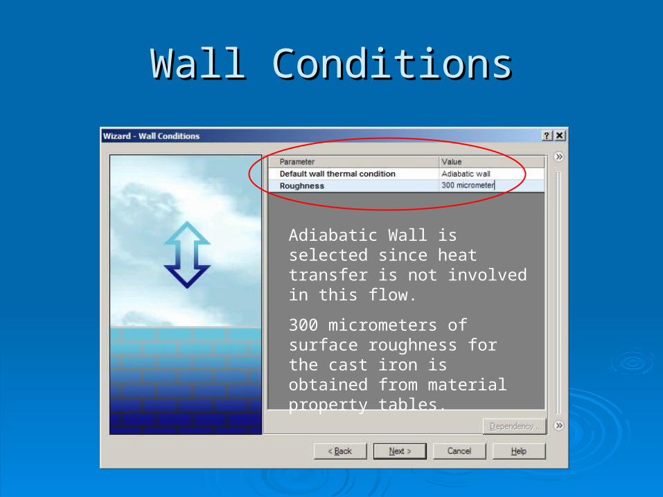
Wall ConditionsWall Conditions

Adiabatic Wall is selected since heat transfer is not involved in this flow.

300 micrometers of surface roughness for the cast iron is obtained from material property tables.

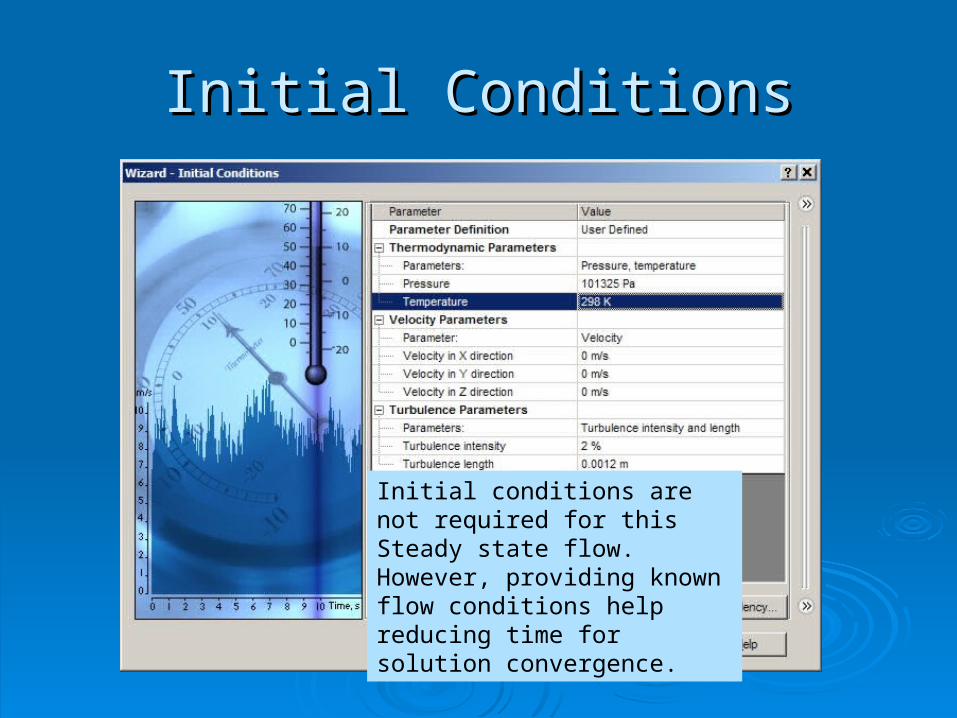
Initial ConditionsInitial Conditions

Initial conditions are not required for this Steady state flow. However, providing known flow conditions help reducing time for solution convergence.

Results and Geometry ResolutionResults and Geometry Resolution

This slide bar will control the mesh size in the solution domain. Higher number setting, i.e., finer meshes may generate better solutions but it requires more CPU time and memory space.

For the initial runs, it is recommended to set it near 3.

Symmetry ConditionSymmetry Condition

Since this model is symmetric, it is possible to “cut” the model in half or in quarter and use a symmetry boundary condition on the plane of symmetry. This procedure is not required but will significantly reduce CPU time and memory space thus more efficient analyses are possible.

Reduced Computational DomainReduced Computational Domain

Applying the symmetry condition reduces the computational domain in half.

11

Specifying the Initial Conditions 1Specifying the Initial Conditions 1

Click FloWorks, Insert, Initial Condition.

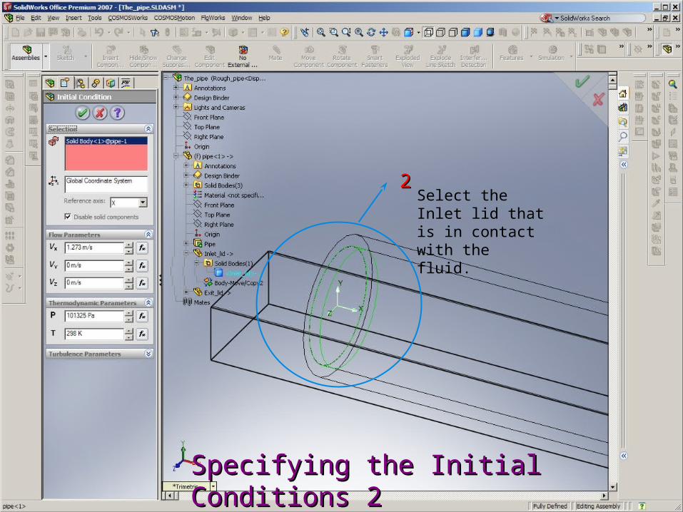
22

Specifying the Initial Conditions 2Specifying the Initial Conditions 2

Select the Inlet lid that is in contact with the fluid.

33

Specifying the Initial Conditions 3Specifying the Initial Conditions 3

Specify known properties of the flow. Inlet Velocity is calculated form inlet volumetric flow rate.

Specifying the Inlet Boundary Conditions 1Specifying the Inlet Boundary Conditions 1

11 Click FloWorks, Insert, Boundary Condition.

Specifying the Inlet Boundary Conditions 2Specifying the Inlet Boundary Conditions 2

22 Select the Inlet lid inner face that is in contact with the fluid

Specifying the Inlet Boundary Conditions 3Specifying the Inlet Boundary Conditions 3

Select, enter Inlet flow properties

33

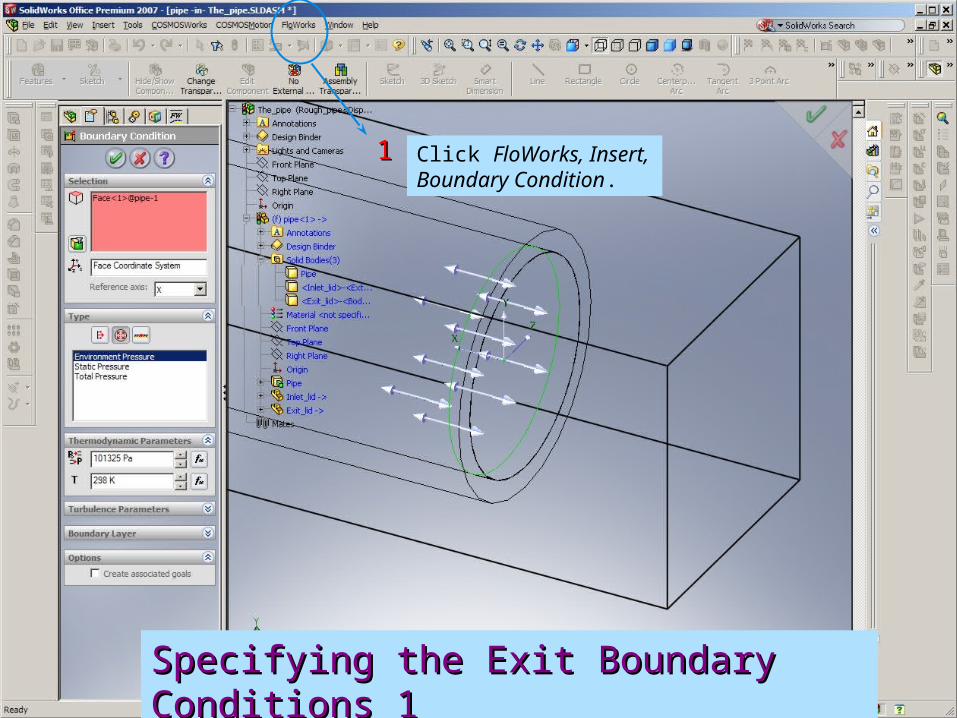
Specifying the Exit Boundary Conditions 1Specifying the Exit Boundary Conditions 1

11 Click FloWorks, Insert, Boundary Condition.

Specifying the Exit Boundary Conditions 2Specifying the Exit Boundary Conditions 2

22

Select the Exit lid inner face that is in contact with the fluid

Specifying the Exit Boundary Conditions 3Specifying the Exit Boundary Conditions 3

33

Click Pressure Openings and choose Static pressure. Enter ambient pressure and the fluid temperature

Running the CalculationRunning the Calculation

Click the FloWorks, Solve, Run. Above Run dialog box appears.

Select Run to start the iteration process

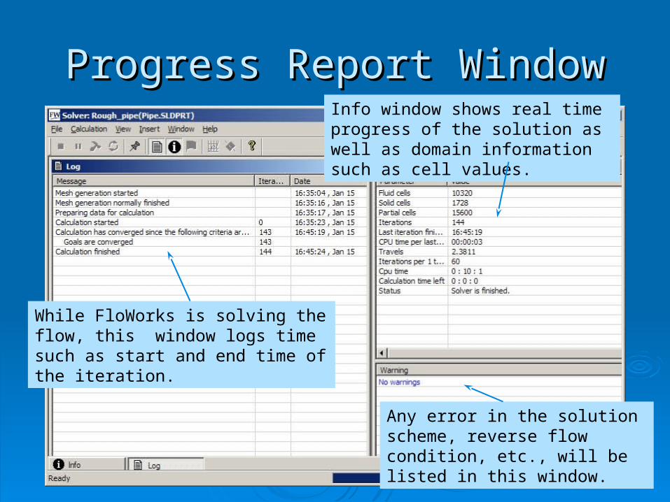
Progress Report WindowProgress Report Window

While FloWorks is solving the flow, this window logs time such as start and end time of the iteration.

Info window shows real time progress of the solution as well as domain information such as cell values.

Any error in the solution scheme, reverse flow condition, etc., will be listed in this window.

CFD Solution AnalysisCFD Solution Analysis

Once iteration is converged, data files are stored with the file extension of *. fdl in the same working folder.

The solution files can be loaded/unloaded by selecting FloWorks, Results, Load/Unload options.

Results such as pressure, velocity, temperature values are shown in both numerical data and graphics form.

Numerical data are useful to obtain local properties of the flow, e.g., pressure drop, while graphical plots show flow behavior in the entire computational domain.

Results SummaryResults Summary

Selecting FloWorks, Results, Results Summary will produce basic information about file structures, computational domain, and flow properties.

From the summary, one can quickly calculate the pressure drop between inlet and exit:

Pmax – Pmin

=103,136.13 – 101,321.38

= 1,814.75 pa

Generating PlotsGenerating Plots

Various flow properties can be shown on different types of plots

Cut plots, Flow Trajectories, Surface plots, Iso-surface plots, Particle plots are most frequently used plot formats.

Cut plot command window is shown by selecting cut plot icon on the main tool bars.

Cut plane can be diagonal, horizontal, or vertical and it can be chosen by selecting a plane in the working window.

Contours, Isolines, and Vectors can be plotted separately or in combinations on one plot.

Cut PlotsCut Plots

Pressure contour is selected to be shown on the cut plot.

Velocity vectors will also be shown on the same cut plot.

Inlet

Exit

Pressure Contour and Velocity Vector Cut PlotPressure Contour and Velocity Vector Cut Plot

Once Cut plot parameters are selected, combinations of flow properties are shown.

Velocity ProfileVelocity Profile

Velocity profiles are shown on the cut plane at the center of the pipe, where Vmin = 0.0m/s, Vmax = 1.54m/s, Vinlet = 1.273m/s.

The flow has not reached to the fully developed stage near the Inlet, while the velocity profiles are consistent along the X-axis: Fully Developed.

Due to the coarseness of the grids near pipe’s inner surface, flow in the boundary layer is not resolved.

Inlet Mid section Exit

Pressure Drop, CFDPressure Drop, CFD

The calculation of the pressure drop, the objective of this simulation, is performed by directly comparing the pressures at the Inlet and the Exit:

P

= Pressure Drop

= Pmin –Pmax

= Pexit – Pinlet

= 101,321.38 – 103,136.13 Pa

= -1,814.75 Pa

= -1.81 kPa

This result is to be compared with the analytic solution for the validation of the computational model.

Calculation of the Friction Factor Calculation of the Friction Factor ff

2 .

2inlet

P df

u L

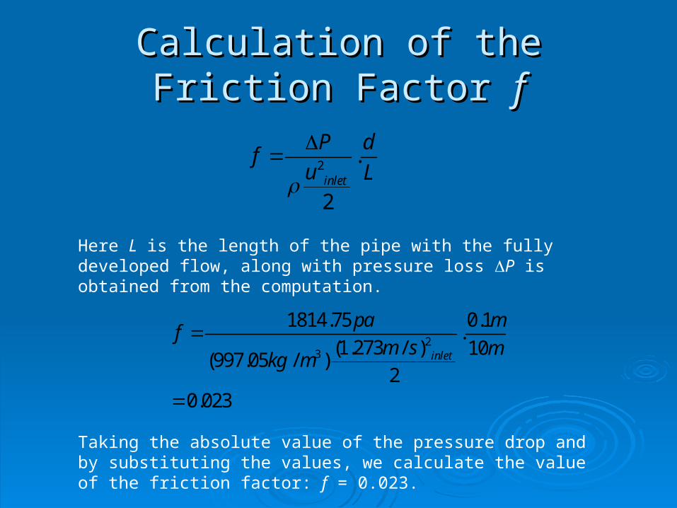
Here L is the length of the pipe with the fully developed flow, along with pressure loss P is obtained from the computation.

23

1814.75 0.1.

(1.273 / ) 10(997.05 / )

20.023

inlet

pa mf

m s mkg m

Taking the absolute value of the pressure drop and by substituting the values, we calculate the value of the friction factor: f = 0.023.

The Reynolds NumberThe Reynolds Number

3

2 2

10 10 /

( / 4)(0.10)1.273 /

m s

mV m s

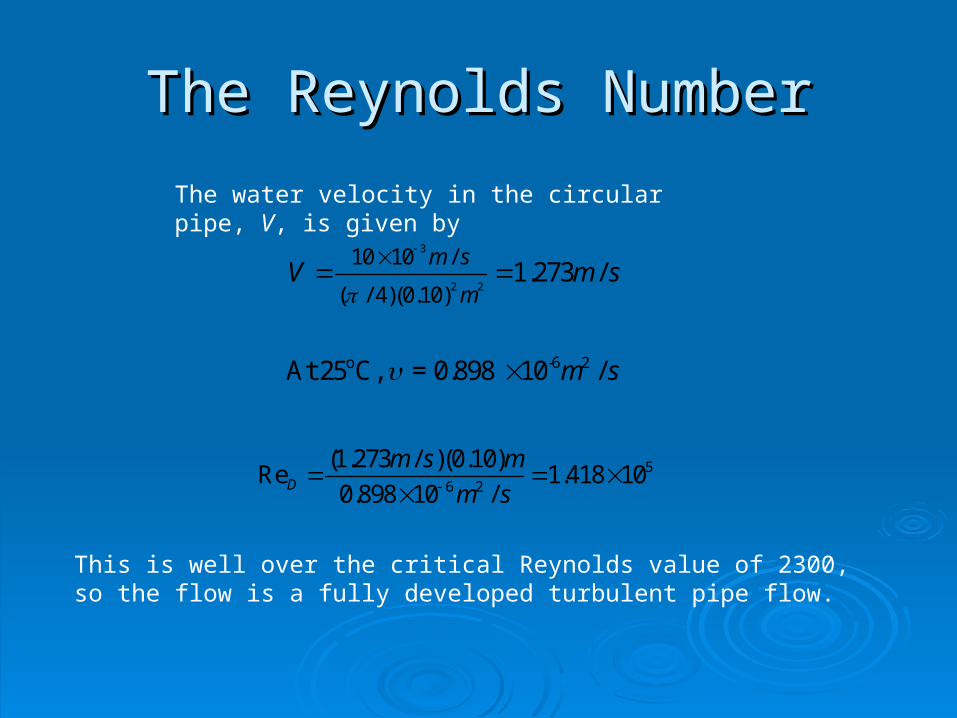
o -6 2At 25 C, = 0.898 10 /m s

56 2

(1.273 / )(0.10)Re 1.418 10

0.898 10 /D

m s m

m s

The water velocity in the circular pipe, V, is given by

This is well over the critical Reynolds value of 2300, so the flow is a fully developed turbulent pipe flow.

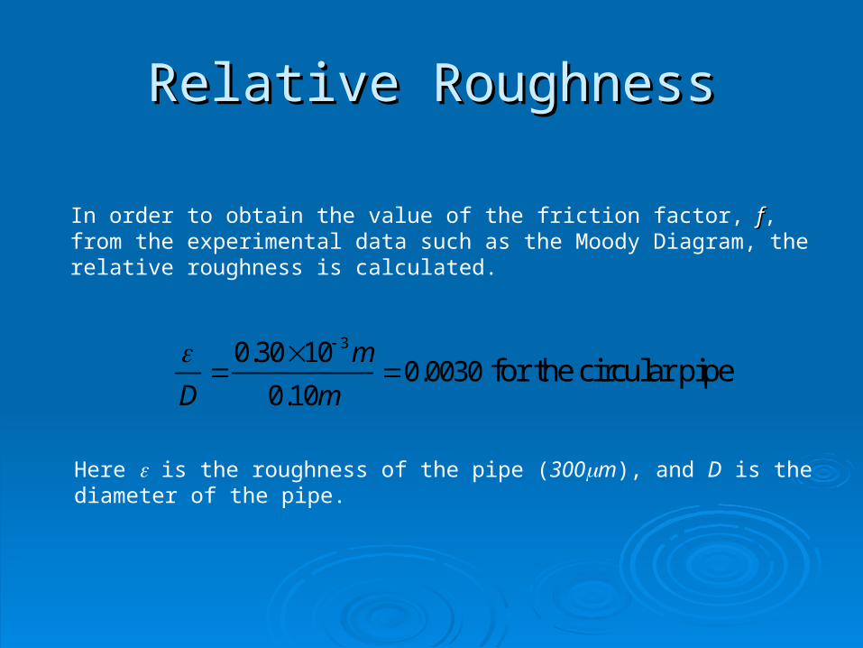
Relative RoughnessRelative Roughness

In order to obtain the value of the friction factor, ff, from the experimental data such as the Moody Diagram, the relative roughness is calculated.

30.30 100.0030

0.10 for the circular pipe

m

D m

Here is the roughness of the pipe (300m), and D is the diameter of the pipe.

Validation of the SolutionValidation of the Solution

The results are to be validated by comparing with: Existing charts such as Moody Diagrams

The moody chart relates the Friction factor for fully developed pipe flow to the Reynolds number and relative roughness of a circular pipe. The relative roughness being , the ratio of the mean height of roughness of the pipe to the pipe diameter.

In 1944, L.F. Moody plotted the Darcy-Weisbach friction factor into what is now known as the Moody DiagramMoody Diagram.

The analytical solutions

The Colebrook Colebrook and Haaland Equations Haaland Equations are implicit equations which combines experimental results of studies of laminar and turbulent flow in pipes.

They were developed in 1939 by C. F. Colebrook, in 1983 by S. E. Haaland, respectively.

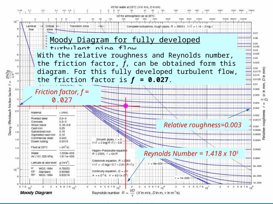
Moody Diagram for fully developed turbulent pipe flow

With the relative roughness and Reynolds number, the friction factor, ff, can be obtained form this diagram. For this fully developed turbulent flow, the friction factor is f = 0.027.

Friction factor, f = 0.027

Relative roughness=0.003

Reynolds Number = 1.418 x 105

Validation Validation using Haaland Equationusing Haaland Equation

0271.0

7.3Re

9.6log8.1

12

f

or

df d

The value of friction factor calculated from Haaland EquationHaaland Equation is in an excellent agreement with the result obtained from Moody Diagram which is based on the Colebrook EquationColebrook Equation.

Validation: Validation: Error CalculationError Calculation

expFriction Factor,

0.027

f

.100 14.8%exp comp

exp

f f

f

Results obtained from Moody Diagram and Haaland Equation:

CFD Solution:

Error:

Friction Factor,

0.023

compf

Sources of DiscrepancySources of Discrepancy

There is a 14.8% difference between Experimental and CFD solutions.

The sources of this discrepancy can be:

Coarse meshes which did not resolve turbulent boundary layers

Lack of refinement / reiteration processes

Inaccurate turbulence model and/or constants

Inlet velocity profile not being fully developed in the CFD simulation (minor)

Coarse MeshesCoarse Meshes

Above plots show the size of the grids and their placement

Inlet, mid-section, and the inclined views from left to right.

Resolution of Level 4 was chosen for the initial configuration, however, to successfully resolve the turbulent buffer and viscous sub-layers smaller grids are to be used near the surface.

To resolve this problem, the automatic mesh generating scheme must be turned off; manually assign grid size and placement for the different flow zones.

Turbulence Solver ModulesTurbulence Solver Modules

To more accurately solve the flow, different Turbulent Kinetic Energy equations and parameters should be tested.

Turbulence intrinsically has uncertainty and thus it is not possible to perfectly predict the turbulent flow as of now.

ConclusionConclusion

Using SolidWorks CAD and COSMOS FloWorks CFD solver suites, a fully developed turbulent pipe flow has been successfully modeled and solved. The roughness of the pipe surface was also accounted for during the solution process.

Although relatively large grids are used, the results obtained from analytic and CFD methods are in good agreement.

Further grid and solver refining is required to obtain better solutions.

AcknowledgmentAcknowledgment

This tutorial was developed under the NSF Grant DUE Number 053619