Friction factor estimation for turbulent flows in corrugatedpipes with rough wallsCitation for published version (APA):Pisarenco, M., Linden, van der, B. J., Tijsseling, A. S., Ory, E., & Dam, J. A. M. (2009). Friction factor estimationfor turbulent flows in corrugated pipes with rough walls. (CASA-report; Vol. 0915). Eindhoven: TechnischeUniversiteit Eindhoven.

Document status and date:Published: 01/01/2009

Document Version:Publisher’s PDF, also known as Version of Record (includes final page, issue and volume numbers)

Please check the document version of this publication:

• A submitted manuscript is the version of the article upon submission and before peer-review. There can beimportant differences between the submitted version and the official published version of record. Peopleinterested in the research are advised to contact the author for the final version of the publication, or visit theDOI to the publisher's website.• The final author version and the galley proof are versions of the publication after peer review.• The final published version features the final layout of the paper including the volume, issue and pagenumbers.Link to publication

General rightsCopyright and moral rights for the publications made accessible in the public portal are retained by the authors and/or other copyright ownersand it is a condition of accessing publications that users recognise and abide by the legal requirements associated with these rights.

• Users may download and print one copy of any publication from the public portal for the purpose of private study or research. • You may not further distribute the material or use it for any profit-making activity or commercial gain • You may freely distribute the URL identifying the publication in the public portal.

If the publication is distributed under the terms of Article 25fa of the Dutch Copyright Act, indicated by the “Taverne” license above, pleasefollow below link for the End User Agreement:www.tue.nl/taverne

Take down policyIf you believe that this document breaches copyright please contact us at:openaccess@tue.nlproviding details and we will investigate your claim.

Download date: 21. Apr. 2020

EINDHOVEN UNIVERSITY OF TECHNOLOGY

Department of Mathematics and Computer Science

CASA-Report 09-15

May 2009

Friction factor estimation for turbulent flows

in corrugated pipes with rough walls

by

M. Pisarenco, B.J. van der Linden,

A.S. Tijssseling, E. Ory, J.A.M. Dam

Centre for Analysis, Scientific computing and Applications

Department of Mathematics and Computer Science

Eindhoven University of Technology

P.O. Box 513

5600 MB Eindhoven, The Netherlands

ISSN: 0926-4507

CASA Report 2009-15

FRICTION FACTOR ESTIMATION FOR TURBULENT FLOWS IN CORRUGATEDPIPES WITH ROUGH WALLS

Maxim Pisarenco ∗

Dept. of Math. and Comp. ScienceEindhoven University of TechnologyP.O. Box 513, 5600 MB Eindhoven

The NetherlandsEmail: m.pisarenco@tue.nl

Bas van der LindenDept. of Math. and Comp. Science

Eindhoven University of TechnologyP.O. Box 513, 5600 MB Eindhoven

The NetherlandsEmail: b.j.v.d.linden@tue.nl

Arris TijsselingDept. of Math. and Comp. Science

Eindhoven University of TechnologyP.O. Box 513, 5600 MB Eindhoven

The NetherlandsEmail: a.s.tijsseling@tue.nl

Emmanuel OrySingle Buoy Moorings Inc.

P.O. Box 199, MC 98007 Monaco CedexMonaco

Email: emmanuel.ory@singlebuoy.com

Jacques DamStork Inoteq

P.O. Box 379, 1000 AJ AmsterdamThe Netherlands

Email: jacques.dam@stork.nl

ABSTRACTThe motivation of the investigation is critical pressure loss

in cryogenic flexible hoses used for LNG transport in offshoreinstallations. Our main goal is to estimate the friction factor forthe turbulent flow in this type of pipes. For this purpose, two-equation turbulence models (k− ε and k−ω) are used in thecomputations.

First, fully developed turbulent flow in a conventional pipeis considered. Simulations are performed to validate the cho-sen models, boundary conditions and computational grids. Thena new boundary condition is implemented based on the “com-bined” law of the wall. It enables us to model the effects ofroughness (and maintain the right flow behavior for moderateReynolds numbers). The implemented boundary condition is val-idated by comparison with experimental data.

Next, turbulent flow in periodically corrugated (flexible)pipes is considered. New flow phenomena (such as flow separa-tion) caused by the corrugation are pointed out and the essenceof periodically fully developed flow is explained. The frictionfactor for different values of relative roughness of the fabric isestimated by performing a set of simulations. Finally, the mainconclusion is presented: the friction factor in a flexible corru-

∗Address all correspondence to this author.

gated pipe is mostly determined by the shape and size of the steelspiral, and not by the type of the fabric which is wrapped aroundthe spiral.Keywords: flexible pipe, friction factor, roughness modeling, cor-rugated pipe, modified law of the wall.

1 INTRODUCTIONNon-metallic flexible pipe products have found wide usage

in industry. Areas of application include heating, ventilation,air-conditioning and, most importantly, connecting terminal ordelivery devices to main distribution ducts (such as transport ofLiquid Natural Gas from ships to the mainland distribution net-work).

Flexible ducts are often comprised of fabric wrapped over aspiral metal framework. Due to this construction, they respondvery well to bending, are cheaper and much easier to install thanmetal pipes. Figure 1 shows a typical flexible pipe. It is con-structed from a neoprene impregnated polyester fabric encapsu-lating a helix spring of steel wire. This tube has an excellentstrength/weight ratio and is able to withstand severe flexing. Thesteel spiral wire gives strength to the pipe, while the use of fab-ric instead of a hard material (such as metal) allows for a highdegree of flexibility.

1

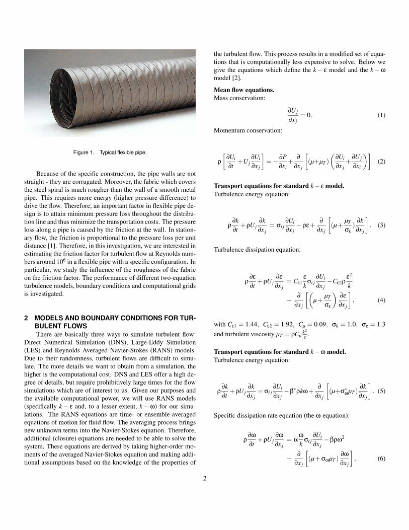
Figure 1. Typical flexible pipe.

Because of the specific construction, the pipe walls are notstraight - they are corrugated. Moreover, the fabric which coversthe steel spiral is much rougher than the wall of a smooth metalpipe. This requires more energy (higher pressure difference) todrive the flow. Therefore, an important factor in flexible pipe de-sign is to attain minimum pressure loss throughout the distribu-tion line and thus minimize the transportation costs. The pressureloss along a pipe is caused by the friction at the wall. In station-ary flow, the friction is proportional to the pressure loss per unitdistance [1]. Therefore, in this investigation, we are interested inestimating the friction factor for turbulent flow at Reynolds num-bers around 106 in a flexible pipe with a specific configuration. Inparticular, we study the influence of the roughness of the fabricon the friction factor. The performance of different two-equationturbulence models, boundary conditions and computational gridsis investigated.

2 MODELS AND BOUNDARY CONDITIONS FOR TUR-BULENT FLOWSThere are basically three ways to simulate turbulent flow:

Direct Numerical Simulation (DNS), Large-Eddy Simulation(LES) and Reynolds Averaged Navier-Stokes (RANS) models.Due to their randomness, turbulent flows are difficult to simu-late. The more details we want to obtain from a simulation, thehigher is the computational cost. DNS and LES offer a high de-gree of details, but require prohibitively large times for the flowsimulations which are of interest to us. Given our purposes andthe available computational power, we will use RANS models(specifically k− ε and, to a lesser extent, k−ω) for our simu-lations. The RANS equations are time- or ensemble-averagedequations of motion for fluid flow. The averaging process bringsnew unknown terms into the Navier-Stokes equation. Therefore,additional (closure) equations are needed to be able to solve thesystem. These equations are derived by taking higher-order mo-ments of the averaged Navier-Stokes equation and making addi-tional assumptions based on the knowledge of the properties of

the turbulent flow. This process results in a modified set of equa-tions that is computationally less expensive to solve. Below wegive the equations which define the k− ε model and the k−ω

model [2].

Mean flow equations.Mass conservation:

∂U j

∂x j= 0. (1)

Momentum conservation:

ρ

[∂Ui

∂t+U j

∂Ui

∂x j

]=− ∂P

∂xi+

∂

∂x j

[(µ+µT )

(∂Ui

∂x j+

∂U j

∂xi

)]. (2)

Transport equations for standard k− ε model.Turbulence energy equation:

ρ∂k∂t

+ρU j∂k∂x j

= σi j∂Ui

∂x j−ρε+

∂

∂x j

[(µ+

µT

σk)

∂k∂x j

]. (3)

Turbulence dissipation equation:

ρ∂ε

∂t+ρU j

∂ε

∂x j= Cε1

ε

kσi j

∂Ui

∂x j−Cε2ρ

ε2

k

+∂

∂x j

[(µ+

µT

σε

)∂ε

∂x j

], (4)

with Cε1 = 1.44, Cε2 = 1.92, Cµ = 0.09, σk = 1.0, σε = 1.3and turbulent viscosity µT = ρCµ

k2

ε.

Transport equations for standard k−ω model.Turbulence energy equation:

ρ∂k∂t

+ρU j∂k∂x j

= σi j∂Ui

∂x j−β

∗ρkω+

∂

∂x j

[(µ+σ

∗ωµT )

∂k∂x j

]. (5)

Specific dissipation rate equation (the ω-equation):

ρ∂ω

∂t+ρU j

∂ω

∂x j= α

ω

kσi j

∂Ui

∂x j−βρω

2

+∂

∂x j

[(µ+σωµT )

∂ω

∂x j

], (6)

2

with α = 59 , β = 3

40 , β∗ = 9100 , σω = 1

2 , σ∗ω = 12 and µT = ρ

kω

.The following notation was used in the Equations (1)-(6):Ui - components of the velocity vector,xi - components of the position vector,t - time,ρ - fluid density,P - pressure,µ - viscosity,µT - turbulent viscosity,k - turbulence kinetic energy,ε - turbulence dissipation,ω - rate of dissipation per unit turbulence kinetic energy,σi j - Reynolds stress tensor, σi j = µT

[∂Ui∂x j

+ ∂U j∂xi

].

These models are given as defined by Wilcox in [2]. It isworth noting here that an updated and improved k−ω model hasbeen presented in 2006 [3]. However, the earlier (standard) ver-sion of the k−ω model was the only option in the used softwarepackage.

The law of the wall. Because of the large velocity gradients aris-ing in the region near the wall, this area requires special treat-ment. Moreover, the flow in the near-wall region is no longerturbulent (at least not everywhere) so that the assumptions madewhile deriving the turbulence models are not valid.

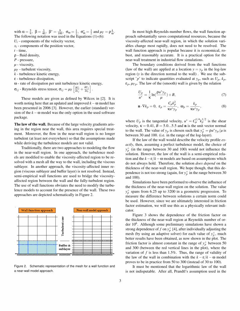
Traditionally, there are two approaches to modeling the flowin the near-wall region. In one approach, the turbulence mod-els are modified to enable the viscosity-affected region to be re-solved with a mesh all the way to the wall, including the viscoussublayer. In another approach, the viscosity-affected inner re-gion (viscous sublayer and buffer layer) is not resolved. Instead,semi-empirical wall functions are used to bridge the viscosity-affected region between the wall and the fully-turbulent region.The use of wall functions obviates the need to modify the turbu-lence models to account for the presence of the wall. These twoapproaches are depicted schematically in Figure 2.

Figure 2. Schematic representation of the mesh for a wall function anda near-wall model approach.

In most high-Reynolds-number flows, the wall function ap-proach substantially saves computational resources, because theviscosity-affected near-wall region, in which the solution vari-ables change most rapidly, does not need to be resolved. Thewall function approach is popular because it is economical, ro-bust, and reasonably accurate. It is a practical option for thenear-wall treatment in industrial flow simulations.

The boundary conditions derived from the wall functions(law of the wall) are applied at a location y = yp in the log-lawregion (y is the direction normal to the wall) . We use the sub-script ’p’ to indicate quantities evaluated at yp, such as Up, kp,εp, µT p. The law of the (smooth) wall is given by the relation

Up

u∗=

1κ

ln(ρu∗yp

µ)+B, (7)

n ·∇kp = 0, εp =Cµk2

p

κu∗yp, ωp =

kp

κu∗yp, (8)

where Up is the tangential velocity, u∗ = C1/4µ k1/2

p is the shearvelocity, κ = 0.41, B = 5.0...5.5 and n is the unit vector normalto the wall. The value of yp is chosen such that y+

p = ρu∗yp/µ isbetween 30 and 100. (i.e. in the range of the log-layer).

If the law of the wall would describe the velocity profile ex-actly, then, assuming a perfect turbulence model, the choice ofy+

p (in the range between 30 and 100) would not influence thesolution. However, the law of the wall is a semi-empirical rela-tion and the k−ε/k−ω models are based on assumptions whichdo not always hold. Therefore, the solution does depend on thethickness of the near-wall region. We hope though, that this de-pendence is not too strong (again, for y+

p in the range between 30and 100).

Simulations have been performed to observe the influence ofthe thickness of the near-wall region on the solution. The valuey+

p spans from 6.25 up to 3200 in a geometric progression. Tomeasure the difference between solutions a certain norm couldbe used. However, since we are ultimately interested in frictionfactor estimation, we will use this as a physically relevant indi-cator.

Figure 3 shows the dependence of the friction factor onthe thickness of the near-wall region at Reynolds number of or-der 106. Although some preliminary simulations have shown astrong dependence of f on y+

p [4], after individually adjusting themesh (by using an adaptive solver) for each value of y+

p , muchbetter results have been obtained, as now shown in the plot. Thefriction factor is almost constant in the range of y+

p between 50and 300 (between the red vertical lines in the plot), where thevariation of f is less than 1.5%. Thus, the range of validity ofthe law of the wall in combination with the k− ε/k−ω modelproves to be in practice from 50 to 300 (instead of 30 to 100).

It must be mentioned that the logarithmic law of the wallis not indisputable. After all, Prandtl’s assumption used in the

3

Figure 3. Dependence of the friction factor f on the thickness y+p of the

near-wall region at Reynolds numbers of order 106. Solid line - computedvalues, dotted line - experimental values (from the Moody diagram). Thek− ε model is used.

derivation of the law is based only on dimensional grounds. Thescaling in the inertial sublayer (also referred to as overlap re-gion) of turbulent wall-bounded flows has long been the sourceof controversy. Barenblatt et al [5] developed theories showingthat power laws are more suitable for describing velocity profilesin wall-bounded turbulent flows. Until recently this controversycould not be addressed because measurements did not span a suf-ficient range of Reynolds number. However, in 1997 new exper-iments conducted by Zaragola et al [6] have shown that at suffi-ciently high Reynolds numbers, the mean velocity profile in theoverlap region is found to be better represented by a log law thana power law. These results suggest a theory of complete simi-larity instead of incomplete similarity, contradicting the theoriesdeveloped by Barenblatt et al.

3 FLOW SIMULATIONS FOR SMOOTH AND ROUGHNON-CORRUGATED PIPESIn this section we evaluate the performance of two-equation

RANS models as implemented in the Finite Element PackageComsol Multiphysics [7] and validate the boundary conditionsbased on the law of the wall which will be used later for morecomplex flows. To do this, we will simulate the turbulent flowin a pipe and assess the validity of the results by comparing thefriction factor computed from the simulation to the one given bythe Moody diagram. Models used in the simulations are k− ε

(Equations (1), (2), (3), (4)) and k−ω (Equations (1), (2), (5),(6)) written in cylindrical coordinates.

Computational domain geometry. The fully devel-oped and time-averaged turbulent flow in a smooth pipe is one-dimensional and axisymmetric in its nature, the only dimensionbeing taken in the radial direction. In the following computa-tions, a 2D axisymmetric model with periodic boundary condi-tions coupling inflow and outflow will be used. See Figure 4.

Boundary conditions. The Axial Symmetry boundarycondition is prescribed at the centerline of the pipe. The otherboundary parallel to the flow coincides with the wall of the pipe.Along this boundary, the law of the wall (7) is used to prescribethe axial velocity at a certain distance from the wall.

An effective method of simulating fully developed flow on asmall computational domain is the use of periodic boundary con-ditions. Their use is explained by the fact that the fully developedflow has a constant velocity profile, which means that:

U1(r,0) = U1(r,L),U2(r,0) = U2(r,L),

k(r,0) = k(r,L), (9)ε(r,0) = ε(r,L),ω(r,0) = ω(r,L).

where L is the length of the computational domain in the axialdirection (set as L = 0.02 m).

At inflow and outflow boundaries we will prescribe constantpressures P(r,0) = Pin and P(r,L) = Pout , where Pout is taken tobe zero. We are entitled to do this because in a fully developedflow through a duct with constant shape cross-section the trans-verse velocity components vanish and it can be easily provenfrom the momentum conservation equation (2) that

∂P∂r

= 0 ⇒ P(r) = constant. (10)

Meshing and solution procedure. Although ourcomputational domain is very regular, which encourages the useof structured meshes, it was decided to use unstructured grids(based on Delaunay triangulation) for the discretization step be-cause we want to use similar grids for both corrugated and non-corrugated pipes, and only unstructured grids can be used for thelatter. The solution procedure consists of three steps:

• Solve the model on a coarse mesh.• Refine the mesh by subdivision to obtain the one shown in

Figure 4.• Solve the model on the refined mesh, using the coarse mesh

solution as an initial guess.

4

inflow

outflow

centerline wall

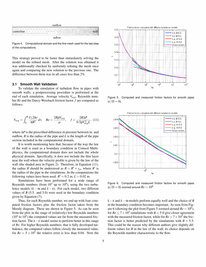
Figure 4. Computational domain and the fine mesh used for the last stepof the computations.

This strategy proved to be faster than immediately solving themodel on the refined mesh. After the solution was obtained itwas additionally checked by uniformly refining the mesh onceagain and comparing the new solution to the previous one. Thedifference between them was in all cases less than 2%.

3.1 Smooth Wall ValidationTo validate the simulation of turbulent flow in pipes with

smooth walls, a postprocessing procedure is performed at theend of each simulation. Average velocity Vavg, Reynolds num-ber Re and the Darcy-Weisbach friction factor f are computed asfollows:

Vavg =Z R

0

U12πrπR2 dr, Re =

2RρVavg

µ, f =

2R∆P0.5ρV 2

avgL, (11)

where ∆P is the prescribed difference in pressure between in- andoutflow, R is the radius of the pipe and L is the length of the pipesection included in the computational domain.

It is worth mentioning here that, because of the way the lawof the wall is used as a boundary condition in Comsol Multi-physics, the computational domain does not include the wholephysical domain. Specifically, it does not include the thin layernear the wall where the velocity profile is given by the law of thewall (the shaded area in Figure 2). Therefore, in Equation (11),the radius R should be understood as R = R′ + yp, where R′ isthe radius of the pipe in the simulations. In the computations thefollowing values have been used: R′ = 0.2 m, L = 0.02 m.

Simulations have been performed for a wide range ofReynolds numbers (from 104 up to 108), using the two turbu-lence models (k−ω and k− ε). For each model, two differentvalues of B (5.5. and 5.0) were used in the boundary conditiongiven by Equation (7).

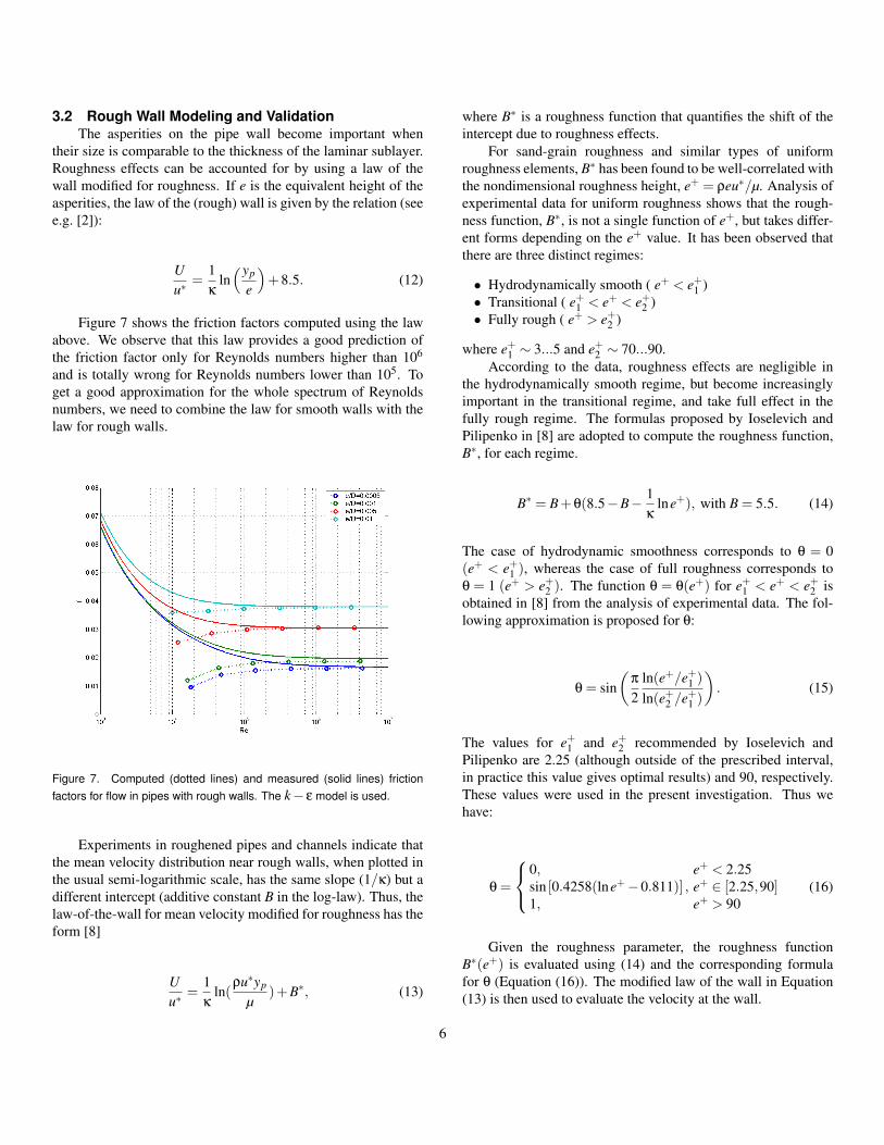
Thus, for each Reynolds number, we end up with four com-puted friction factors plus the friction factor taken from theMoody diagram. These are shown in Figure 5. As can be seenfrom the plot, in the range of (relatively) low Reynolds numbers(104 to 105) the computed values are far from the measured fric-tion factor. The k−ε model seems to perform better in this rangeof Re. For higher Reynolds numbers, that is fully developed tur-bulence, the computed values follow closely the measured value;for Re > 5× 105 the relative error is less than 0.04. Now the

Figure 5. Computed and measured friction factors for smooth pipes(e/D = 0).

Figure 6. Computed and measured friction factors for smooth pipes(e/D = 0) zoomed around Re ∼ 106.

k−ε and k−ω models perform equally well and the choice of Bin the boundary condition becomes important. As seen from Fig-ure 6 (showing the plot from Figure 5 zoomed around Re = 106),for Re≤ 7×105 simulations with B = 5.0 give closer agreementwith the measured friction factor, while for Re > 7×105 the fric-tion factor is better predicted by the simulations with B = 5.5.This could be the reason why different authors give slightly dif-ferent values for B in the law of the wall; its choice depends onthe Reynolds number characteristic to the flow.

5

3.2 Rough Wall Modeling and ValidationThe asperities on the pipe wall become important when

their size is comparable to the thickness of the laminar sublayer.Roughness effects can be accounted for by using a law of thewall modified for roughness. If e is the equivalent height of theasperities, the law of the (rough) wall is given by the relation (seee.g. [2]):

Uu∗

=1κ

ln(yp

e

)+8.5. (12)

Figure 7 shows the friction factors computed using the lawabove. We observe that this law provides a good prediction ofthe friction factor only for Reynolds numbers higher than 106

and is totally wrong for Reynolds numbers lower than 105. Toget a good approximation for the whole spectrum of Reynoldsnumbers, we need to combine the law for smooth walls with thelaw for rough walls.

Figure 7. Computed (dotted lines) and measured (solid lines) frictionfactors for flow in pipes with rough walls. The k− ε model is used.

Experiments in roughened pipes and channels indicate thatthe mean velocity distribution near rough walls, when plotted inthe usual semi-logarithmic scale, has the same slope (1/κ) but adifferent intercept (additive constant B in the log-law). Thus, thelaw-of-the-wall for mean velocity modified for roughness has theform [8]

Uu∗

=1κ

ln(ρu∗yp

µ)+B∗, (13)

where B∗ is a roughness function that quantifies the shift of theintercept due to roughness effects.

For sand-grain roughness and similar types of uniformroughness elements, B∗ has been found to be well-correlated withthe nondimensional roughness height, e+ = ρeu∗/µ. Analysis ofexperimental data for uniform roughness shows that the rough-ness function, B∗, is not a single function of e+, but takes differ-ent forms depending on the e+ value. It has been observed thatthere are three distinct regimes:

• Hydrodynamically smooth ( e+ < e+1 )

• Transitional ( e+1 < e+ < e+

2 )• Fully rough ( e+ > e+

2 )

where e+1 ∼ 3...5 and e+

2 ∼ 70...90.According to the data, roughness effects are negligible in

the hydrodynamically smooth regime, but become increasinglyimportant in the transitional regime, and take full effect in thefully rough regime. The formulas proposed by Ioselevich andPilipenko in [8] are adopted to compute the roughness function,B∗, for each regime.

B∗ = B+θ(8.5−B− 1κ

lne+), with B = 5.5. (14)

The case of hydrodynamic smoothness corresponds to θ = 0(e+ < e+

1 ), whereas the case of full roughness corresponds toθ = 1 (e+ > e+

2 ). The function θ = θ(e+) for e+1 < e+ < e+

2 isobtained in [8] from the analysis of experimental data. The fol-lowing approximation is proposed for θ:

θ = sin(

π

2ln(e+/e+

1 )ln(e+

2 /e+1 )

). (15)

The values for e+1 and e+

2 recommended by Ioselevich andPilipenko are 2.25 (although outside of the prescribed interval,in practice this value gives optimal results) and 90, respectively.These values were used in the present investigation. Thus wehave:

θ =

0, e+ < 2.25sin [0.4258(lne+−0.811)] , e+ ∈ [2.25,90]1, e+ > 90

(16)

Given the roughness parameter, the roughness functionB∗(e+) is evaluated using (14) and the corresponding formulafor θ (Equation (16)). The modified law of the wall in Equation(13) is then used to evaluate the velocity at the wall.

6

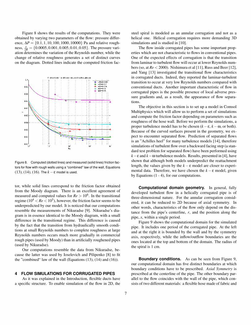
Figure 8 shows the results of the computations. They wereobtained by varying two parameters of the flow: pressure differ-ence, ∆P = {0.1,1,10,100,1000,10000} Pa and relative rough-ness, e

2R = {0.0005,0.001,0.005,0.01,0.05}. The pressure vari-ation determines the variation of the Reynolds number, while thechange of relative roughness generates a set of distinct curveson the diagram. Dotted lines indicate the computed friction fac-

Figure 8. Computed (dotted lines) and measured (solid lines) friction fac-tors for flow with rough walls using a “combined” law of the wall, Equations(13), (14), (16). The k− ε model is used.

tor, while solid lines correspond to the friction factor obtainedfrom the Moody diagram. There is an excellent agreement ofmeasured and computed values for Re > 106. In the transitionalregime (104 < Re < 105), however, the friction factor seems to beunderpredicted by our model. It is noticed that our computationsresemble the measurements of Nikuradse [9]. Nikuradse’s dia-gram is in essence identical to the Moody diagram, with a smalldifference in the transitional regime. This difference is causedby the fact that the transition from hydraulically smooth condi-tions at small Reynolds numbers to complete roughness at largeReynolds numbers occurs much more gradually in commercialrough pipes (used by Moody) than in artificially roughened pipes(used by Nikuradse).

Our computations resemble the data from Nikuradse, be-cause the latter was used by Ioselevich and Pilipenko [8] to fitthe ”combined“ law of the wall (Equations (13), (14) and (16)).

4 FLOW SIMULATIONS FOR CORRUGATED PIPESAs it was explained in the Introduction, flexible ducts have

a specific structure. To enable simulation of the flow in 2D, the

steel spiral is modeled as an annular corrugation and not as ahelical one. Helical corrugation requires more demanding 3Dsimulations and is studied in [10].

The flow inside corrugated pipes has some important prop-erties which are not characteristic to flows in conventional pipes.One of the expected effects of corrugation is that the transitionfrom laminar to turbulent flow will occur at lower Reynolds num-bers (so, at Re < 2000). Nishimura et al [11], Russ and Beer [12],and Yang [13] investigated the transitional flow characteristicsin corrugated ducts. Indeed, they reported the laminar-turbulenttransition to occur at very low Reynolds numbers compared withconventional ducts. Another important characteristic of flow incorrugated pipes is the possible presence of local adverse pres-sure gradients and, as a result, the appearance of flow separa-tions.

The objective in this section is to set up a model in ComsolMultiphysics which will allow us to perform a set of simulationsand compute the friction factor depending on parameters such asroughness of the hose wall. Before we perform the simulations, aproper turbulence model has to be chosen (k− ε, k−ω, or both).Because of the curved surfaces present in the geometry, we ex-pect to encounter separated flow. Prediction of separated flowsis an ”Achilles heel” for many turbulence models [14], thereforesimulations of turbulent flow over a backward facing step (a stan-dard test problem for separated flow) have been performed usingk−ε and k−ω turbulence models. Results, presented in [4], haveshown that although both models underpredict the reattachmentlength, the values given by the k− ε model are closer to experi-mental data. Therefore, we have chosen the k− ε model, givenby Equations (1 - 4), for our computations.

Computational domain geometry. In general, fullydeveloped turbulent flow in a helically corrugated pipe is ofthree-dimensional nature. For the annular corrugation consid-ered, it can be reduced to 2D because of axial symmetry. Inother words, characteristics of the flow only depend on the dis-tance from the pipe’s centerline, r, and the position along thepipe, x, within a single period.

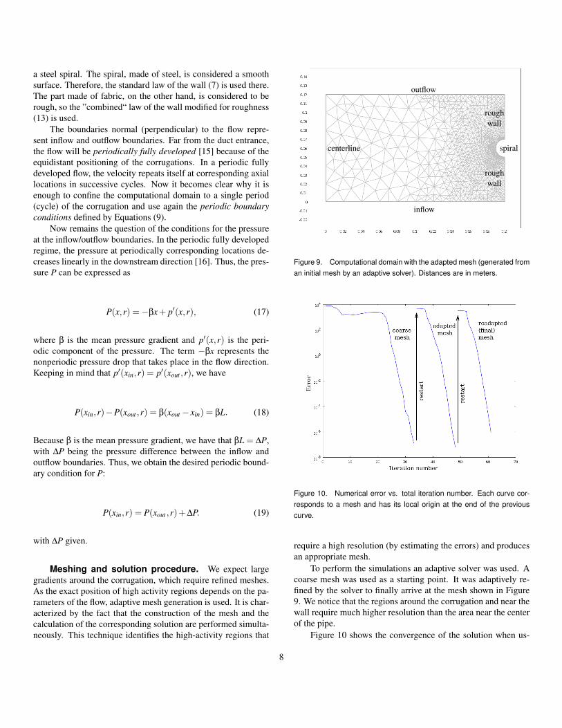
Figure 9 shows the computational domain for the simulatedpipe. It includes one period of the corrugated pipe. At the leftand at the right it is bounded by the wall and by the symmetryaxis, respectively, while the inflow/outflow boundaries are theones located at the top and bottom of the domain. The radius ofthe spiral is 1 cm.

Boundary conditions. As can be seen from Figure 9,our computational domain has five distinct boundaries at whichboundary conditions have to be prescribed. Axial Symmetry isprescribed at the centerline of the pipe. The other boundary par-allel to the flow coincides with the wall of the pipe, which con-sists of two different materials: a flexible hose made of fabric and

7

a steel spiral. The spiral, made of steel, is considered a smoothsurface. Therefore, the standard law of the wall (7) is used there.The part made of fabric, on the other hand, is considered to berough, so the ”combined“ law of the wall modified for roughness(13) is used.

The boundaries normal (perpendicular) to the flow repre-sent inflow and outflow boundaries. Far from the duct entrance,the flow will be periodically fully developed [15] because of theequidistant positioning of the corrugations. In a periodic fullydeveloped flow, the velocity repeats itself at corresponding axiallocations in successive cycles. Now it becomes clear why it isenough to confine the computational domain to a single period(cycle) of the corrugation and use again the periodic boundaryconditions defined by Equations (9).

Now remains the question of the conditions for the pressureat the inflow/outflow boundaries. In the periodic fully developedregime, the pressure at periodically corresponding locations de-creases linearly in the downstream direction [16]. Thus, the pres-sure P can be expressed as

P(x,r) =−βx+ p′(x,r), (17)

where β is the mean pressure gradient and p′(x,r) is the peri-odic component of the pressure. The term −βx represents thenonperiodic pressure drop that takes place in the flow direction.Keeping in mind that p′(xin,r) = p′(xout ,r), we have

P(xin,r)−P(xout ,r) = β(xout − xin) = βL. (18)

Because β is the mean pressure gradient, we have that βL = ∆P,with ∆P being the pressure difference between the inflow andoutflow boundaries. Thus, we obtain the desired periodic bound-ary condition for P:

P(xin,r) = P(xout ,r)+∆P. (19)

with ∆P given.

Meshing and solution procedure. We expect largegradients around the corrugation, which require refined meshes.As the exact position of high activity regions depends on the pa-rameters of the flow, adaptive mesh generation is used. It is char-acterized by the fact that the construction of the mesh and thecalculation of the corresponding solution are performed simulta-neously. This technique identifies the high-activity regions that

inflow

outflow

roughwall

roughwall

centerline spiral

Figure 9. Computational domain with the adapted mesh (generated froman initial mesh by an adaptive solver). Distances are in meters.

Figure 10. Numerical error vs. total iteration number. Each curve cor-responds to a mesh and has its local origin at the end of the previouscurve.

require a high resolution (by estimating the errors) and producesan appropriate mesh.

To perform the simulations an adaptive solver was used. Acoarse mesh was used as a starting point. It was adaptively re-fined by the solver to finally arrive at the mesh shown in Figure9. We notice that the regions around the corrugation and near thewall require much higher resolution than the area near the centerof the pipe.

Figure 10 shows the convergence of the solution when us-

8

ing the adaptive solver. First, the model is solved on the coarsemesh. Then the errors are estimated and the mesh is refined atthe locations with the larger errors. The model is solved again onthe new mesh.The process continues until the errors are smallerthan a certain threshold and the maximum number of mesh re-finements is reached (this number is 2 in our case).

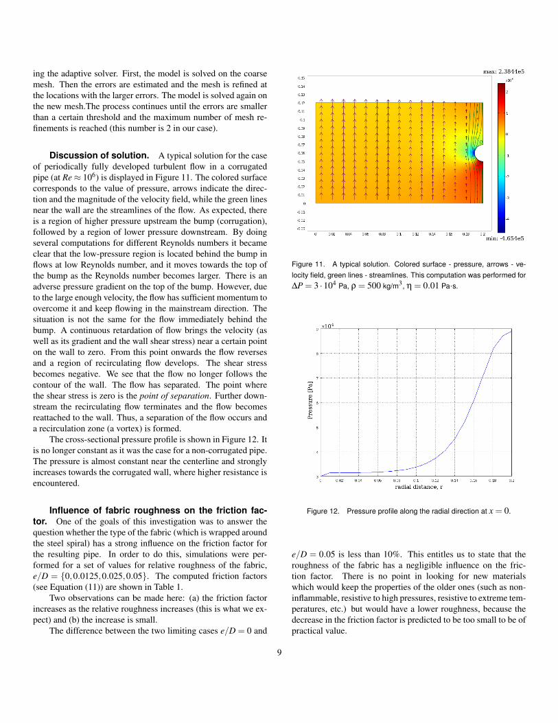
Discussion of solution. A typical solution for the caseof periodically fully developed turbulent flow in a corrugatedpipe (at Re≈ 106) is displayed in Figure 11. The colored surfacecorresponds to the value of pressure, arrows indicate the direc-tion and the magnitude of the velocity field, while the green linesnear the wall are the streamlines of the flow. As expected, thereis a region of higher pressure upstream the bump (corrugation),followed by a region of lower pressure downstream. By doingseveral computations for different Reynolds numbers it becameclear that the low-pressure region is located behind the bump inflows at low Reynolds number, and it moves towards the top ofthe bump as the Reynolds number becomes larger. There is anadverse pressure gradient on the top of the bump. However, dueto the large enough velocity, the flow has sufficient momentum toovercome it and keep flowing in the mainstream direction. Thesituation is not the same for the flow immediately behind thebump. A continuous retardation of flow brings the velocity (aswell as its gradient and the wall shear stress) near a certain pointon the wall to zero. From this point onwards the flow reversesand a region of recirculating flow develops. The shear stressbecomes negative. We see that the flow no longer follows thecontour of the wall. The flow has separated. The point wherethe shear stress is zero is the point of separation. Further down-stream the recirculating flow terminates and the flow becomesreattached to the wall. Thus, a separation of the flow occurs anda recirculation zone (a vortex) is formed.

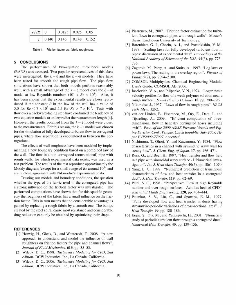
The cross-sectional pressure profile is shown in Figure 12. Itis no longer constant as it was the case for a non-corrugated pipe.The pressure is almost constant near the centerline and stronglyincreases towards the corrugated wall, where higher resistance isencountered.

Influence of fabric roughness on the friction fac-tor. One of the goals of this investigation was to answer thequestion whether the type of the fabric (which is wrapped aroundthe steel spiral) has a strong influence on the friction factor forthe resulting pipe. In order to do this, simulations were per-formed for a set of values for relative roughness of the fabric,e/D = {0,0.0125,0.025,0.05}. The computed friction factors(see Equation (11)) are shown in Table 1.

Two observations can be made here: (a) the friction factorincreases as the relative roughness increases (this is what we ex-pect) and (b) the increase is small.

The difference between the two limiting cases e/D = 0 and

Figure 11. A typical solution. Colored surface - pressure, arrows - ve-locity field, green lines - streamlines. This computation was performed for∆P = 3 ·104 Pa, ρ = 500 kg/m3, η = 0.01 Pa·s.

Figure 12. Pressure profile along the radial direction at x = 0.

e/D = 0.05 is less than 10%. This entitles us to state that theroughness of the fabric has a negligible influence on the fric-tion factor. There is no point in looking for new materialswhich would keep the properties of the older ones (such as non-inflammable, resistive to high pressures, resistive to extreme tem-peratures, etc.) but would have a lower roughness, because thedecrease in the friction factor is predicted to be too small to be ofpractical value.

9

e/2R 0 0.0125 0.025 0.05

f 0.140 0.146 0.148 0.152

Table 1. Friction factor vs. fabric roughness.

5 CONCLUSIONSThe performance of two-equation turbulence models

(RANS) was assessed. Two popular representatives of this classwere investigated: the k− ε and the k−ω models. They havebeen tested for smooth and rough pipe flow. The pipe flowsimulations have shown that both models perform reasonablywell, with a small advantage of the k− ε model over the k−ω

model at low Reynolds numbers (104 < Re < 105). Also, ithas been shown that the experimental results are closer repro-duced if the constant B in the law of the wall has a value of5.0 for Re ≤ 7× 105 and 5.5 for Re > 7× 105. Tests withflow over a backward-facing step have confirmed the tendency oftwo-equation models to underpredict the reattachment length [4].However, the results obtained from the k− ε model were closerto the measurements. For this reason, the k−ε model was chosenfor the simulation of fully developed turbulent flow in corrugatedpipes, where flow separation is encountered in between the cor-rugations.

The effects of wall roughness have been modeled by imple-menting a new boundary condition based on a combined law ofthe wall. The flow in a non-corrugated (conventional) pipe withrough walls, for which experimental data exists, was used as atest problem. The results of the test reproduce approximately theMoody diagram (except for a small range of Re around 105) andare in close agreement with Nikuradse’s experimental data.

Trusting our models and boundary conditions, the questionwhether the type of the fabric used in the corrugated pipe hasa strong influence on the friction factor was investigated. Theperformed computations have shown that for this specific geom-etry the roughness of the fabric has a small influence on the fric-tion factor. This in turn means that no considerable advantage isgained by replacing a rough fabric by a smooth one. The bumpscreated by the steel spiral cause most resistance and considerabledrag reduction can only be obtained by optimizing their shape.

REFERENCES[1] Herwig, H., Gloss, D., and Wenterodt, T., 2008. “A new

approach to understand and model the influence of wallroughness on friction factors for pipe and channel flows”.Journal of Fluid Mechanics, 613, pp. 35–53.

[2] Wilcox, D. C., 1998. Turbulence Modeling for CFD, 2ndedition. DCW Industries, Inc., La Canada, California.

[3] Wilcox, D. C., 2006. Turbulence Modeling for CFD, 3ndedition. DCW Industries, Inc., La Canada, California.

[4] Pisarenco, M., 2007. “Friction factor estimation for turbu-lent flows in corrugated pipes with rough walls”. Master’sthesis, Eindhoven University of Technology.

[5] Barenblatt, G. I., Chorin, A. J., and Prostokishin, V. M.,1997. “Scaling laws for fully developed turbulent flow inpipes: discussion of experimental data”. Proceedings of theNational Academy of Sciences of the USA, 94(3), pp. 773–776.

[6] Zagarola, M., Perry, A., and Smits, A., 1997. “Log laws orpower laws: The scaling in the overlap region”. Physics ofFluids, 9(7), pp. 2094–2100.

[7] COMSOL Multiphysics. Chemical Engineering Module,User’s Guide. COMSOL AB, 2006.

[8] Ioselevich, V. A., and Pilipenko, V. N., 1974. “Logarithmicvelocity profiles for flow of a weak polymer solution near arough surface”. Soviet Physics Doklady, 18, pp. 790–796.

[9] Nikuradse, J., 1937. “Laws of flow in rough pipes”. NACATech. Mem. 1292.

[10] van der Linden, B., Pisarenco, M., Ory, E., Dam, J., andTijsseling, A., 2009. “Efficient computation of three-dimensional flow in helically corrugated hoses includingswirl”. Proc. of the 2009 ASME Pressure Vessels and Pip-ing Division Conf., Prague, Czech Republic, July 2009, Pa-per PVP2009-77997. Accepted.

[11] Nishimura, T., Ohori, Y., and Kawamura, Y., 1984. “Flowcharacteristics in a channel with symmetric wavy wall forsteady flow”. J. Chem. Eng. of Japan, 17, pp. 466–471.

[12] Russ, G., and Beer, H., 1997. “Heat transfer and flow fieldin a pipe with sinusoidal wavy surface - I. Numerical inves-tigation”. Int. J. Heat Mass Transfer, 40(5), pp. 1061–1070.

[13] Yang, L. C., 1997. “Numerical prediction of transitionalcharacteristics of flow and heat transfer in a corrugatedduct”. J. Heat Transfer, 119, pp. 62–69.

[14] Patel, V. C., 1998. “Perspective: Flow at high Reynoldsnumber and over rough surfaces - Achilles heel of CFD”.Journal of Fluids Engineering, 120, pp. 434–444.

[15] Patankar, S. V., Liu, C., and Sparrow, E. M., 1977.“Fully developed flow and heat transfer in ducts havingstreamwise-periodic variations of cross-sectional area”. J.Heat Transfer, 99, pp. 180–186.

[16] Ergin, S., Ota, M., and Yamaguchi, H., 2001. “Numericalstudy of periodic turbulent flow through a corrugated duct”.Numerical Heat Transfer, 40, pp. 139–156.

10

PREVIOUS PUBLICATIONS IN THIS SERIES:

Number Author(s) Title Month

09-11

09-12

09-13

09-14

09-15

A.Muntean

L.M.J. Florack

J.A.W.M. Groot

C.G. Giannopapa

R.M.M. Mattheij

A.S. Tijsseling

M. Pisarenco

B.J. van der Linden

A.S. Tijssseling

E. Ory

J.A.M. Dam

Large-time behavior of

solutions to a reaction-

diffusion system with

distributed microstructure

Coarse-to-fine partitioning of

signals

Numerical optimisation of

blowing glass parison shapes

Exact computation of the

axial vibration of two coupled

liquid-filled pipes

Friction factor estimation for

turbulent flows in corrugated

pipes with rough walls

March ‘09

March ‘09

March ‘09

May ‘09

May ‘09

Ontwerp: de Tantes,

Tobias Baanders, CWI