freshman physics laboratory physics 3 course experiments - ligo

DRAFT

PHYSICS MATHEMATICS AND ASTRONOMY DIVISION

CALIFORNIA INSTITUTE OF TECHNOLOGY

Freshman Physics Laboratory

Physics 3 Course

Experiments NotesAcademic Year 2012-2013

( Minor Revision September 2012)

Virgınio de Oliveira Sannibale, Kenneth G. Libbrecht

Caltech Physics Deparment, MS 103-331200 E. California Blvd.

91125 Pasadena,CAhttp://www.ligo.caltech.edu/˜vsanni/ph3/

DRAFT

2

DRAFT

Contents

1 Data Analysis 7

2 The Maxwell Top 112.1 Introduction . . . . . . . . . . . . . . . . . . . . . . . . . . . . 112.2 Some Relevant Examples . . . . . . . . . . . . . . . . . . . . . 12

2.2.1 Angular Acceleration under a Constant Torque . . . 122.2.2 Top Suspended with a Torsional Rod . . . . . . . . . 132.2.3 Precession of the Top . . . . . . . . . . . . . . . . . . 14

2.3 Experimental setup. . . . . . . . . . . . . . . . . . . . . . . . . 162.3.1 Care and Use of the Experimental Apparatus . . . . . 16

2.4 First Laboratory Week . . . . . . . . . . . . . . . . . . . . . . 182.4.1 Indirect Measurement of the Moment of Inertia Ap-

plying a Constant Torque . . . . . . . . . . . . . . . . 182.4.2 Indirect Measurement of the Moment of Inertia Us-

ing a Torsional Pendulum . . . . . . . . . . . . . . . . 182.4.3 Propaedeutic Problems . . . . . . . . . . . . . . . . . 192.4.4 Procedure ( Top’s Moment of Inertia Measurements) 19

2.5 Second Laboratory Week . . . . . . . . . . . . . . . . . . . . . 212.5.1 Propaedeutic Problems. . . . . . . . . . . . . . . . . . 222.5.2 Procedure (Precession Period Measurement) . . . . . 23

3 The Inverted Pendulum 253.1 Introduction . . . . . . . . . . . . . . . . . . . . . . . . . . . . 253.2 Modeling the Inverted Pendulum (IP) . . . . . . . . . . . . . 26

3.2.1 The Simple Harmonic Oscillator . . . . . . . . . . . . 263.2.2 The Simple Pendulum . . . . . . . . . . . . . . . . . . 263.2.3 The Simple Inverted Pendulum . . . . . . . . . . . . . 273.2.4 A Better Model of the Inverted Pendulum . . . . . . . 29

3

DRAFT

4 CONTENTS

3.3 The Damped Harmonic Oscillator . . . . . . . . . . . . . . . 303.4 The Driven Harmonic Oscillator . . . . . . . . . . . . . . . . 313.5 The Transfer Function . . . . . . . . . . . . . . . . . . . . . . 333.6 The Inverted Pendulum Test Bench . . . . . . . . . . . . . . . 34

3.6.1 Care and Use of the Apparatus . . . . . . . . . . . . . 343.7 The Lab - First Week . . . . . . . . . . . . . . . . . . . . . . . 34

3.7.1 Pre-Lab Problems . . . . . . . . . . . . . . . . . . . . . 343.7.2 In-Lab Exercises . . . . . . . . . . . . . . . . . . . . . . 35

3.7.2.1 Getting Started . . . . . . . . . . . . . . . . . 353.7.2.2 The IP Leg . . . . . . . . . . . . . . . . . . . 363.7.2.3 Resonant Frequency versus Load . . . . . . 36

3.8 The Lab - Second Week . . . . . . . . . . . . . . . . . . . . . . 393.8.1 Pre-Lab Problems . . . . . . . . . . . . . . . . . . . . . 393.8.2 In-Lab Exercises . . . . . . . . . . . . . . . . . . . . . . 40

3.8.2.1 Inverted Pendulum Loss Angle . . . . . . . 403.8.2.2 The Transfer Function . . . . . . . . . . . . . 40

3.9 EndNote: Using Complex Functions to Solve Real Equations 41

4 Direct Current Network Theory 434.1 Electronic Networks . . . . . . . . . . . . . . . . . . . . . . . 43

4.1.1 Network Definitions . . . . . . . . . . . . . . . . . . . 434.1.2 Series and Parallel . . . . . . . . . . . . . . . . . . . . 444.1.3 Active and Passive Components . . . . . . . . . . . . 45

4.2 Kirchhoff’s Laws . . . . . . . . . . . . . . . . . . . . . . . . . 454.3 Resistors (Ohm’s Law) . . . . . . . . . . . . . . . . . . . . . . 45

4.3.1 Resistors in Series . . . . . . . . . . . . . . . . . . . . . 464.3.2 Resistors in Parallel . . . . . . . . . . . . . . . . . . . . 47

4.4 Capacitors . . . . . . . . . . . . . . . . . . . . . . . . . . . . . 484.4.1 Capacitors in Parallel . . . . . . . . . . . . . . . . . . . 484.4.2 Capacitors in Series . . . . . . . . . . . . . . . . . . . . 49

4.5 Ideal and Real Sources . . . . . . . . . . . . . . . . . . . . . . 504.5.1 Ideal Voltage Source . . . . . . . . . . . . . . . . . . . 504.5.2 Ideal Current Source . . . . . . . . . . . . . . . . . . . 50

4.6 The Semiconductor Junction (Diode) . . . . . . . . . . . . . . 514.7 Equivalent Networks . . . . . . . . . . . . . . . . . . . . . . . 53

4.7.1 Voltage Divider . . . . . . . . . . . . . . . . . . . . . . 534.7.2 Thevenin Theorem . . . . . . . . . . . . . . . . . . . . 544.7.3 Norton Theorem . . . . . . . . . . . . . . . . . . . . . 56

DRAFT

CONTENTS 5

4.8 Resistor Color Code . . . . . . . . . . . . . . . . . . . . . . . . 564.9 First Laboratory Week . . . . . . . . . . . . . . . . . . . . . . 58

4.9.1 Pre-Laboratory Problems . . . . . . . . . . . . . . . . 594.9.2 Procedure . . . . . . . . . . . . . . . . . . . . . . . . . 60

4.10 Second Laboratory Week . . . . . . . . . . . . . . . . . . . . . 624.10.1 Pre-Laboratory Problems . . . . . . . . . . . . . . . . 624.10.2 Procedure . . . . . . . . . . . . . . . . . . . . . . . . . 63

5 Alternating Current Network Theory 655.1 Symbolic Representation of a Sinusoidal Signals, Phasors . . 65

5.1.1 Derivative of a Phasor . . . . . . . . . . . . . . . . . . 675.1.2 Integral of a Phasor . . . . . . . . . . . . . . . . . . . . 67

5.2 Current Voltage Equation for Passive Ideal Components withPhasors . . . . . . . . . . . . . . . . . . . . . . . . . . . . . . . 675.2.1 The Resistor . . . . . . . . . . . . . . . . . . . . . . . . 685.2.2 The Capacitor . . . . . . . . . . . . . . . . . . . . . . . 685.2.3 The Inductor . . . . . . . . . . . . . . . . . . . . . . . 69

5.3 The Impedance and Admittance Concept. . . . . . . . . . . . 705.3.1 Impedance in Parallel and Series . . . . . . . . . . . . 715.3.2 Ohm’s Law for Sinusoidal Regime . . . . . . . . . . . 71

5.4 Two-port Network . . . . . . . . . . . . . . . . . . . . . . . . 715.4.1 The RC Low-Pass Filter . . . . . . . . . . . . . . . . . 735.4.2 The CR High-Pass Filter . . . . . . . . . . . . . . . . . 745.4.3 The LCR Series Resonant Circuit . . . . . . . . . . . . 76

5.5 First Laboratory Week . . . . . . . . . . . . . . . . . . . . . . 795.5.1 Pre-laboratory Exercises . . . . . . . . . . . . . . . . . 795.5.2 Procedure . . . . . . . . . . . . . . . . . . . . . . . . . 80

5.6 Second Laboratory Week . . . . . . . . . . . . . . . . . . . . . 825.6.1 Pre-laboratory Exercises . . . . . . . . . . . . . . . . . 825.6.2 Procedure . . . . . . . . . . . . . . . . . . . . . . . . . 83

A Measurements and Significant Figures(Draft) 87A.1 Scientific Notation . . . . . . . . . . . . . . . . . . . . . . . . . 87A.2 Significant Figures . . . . . . . . . . . . . . . . . . . . . . . . 88A.3 Significant Figures in Measurements . . . . . . . . . . . . . . 88

A.3.1 Significant Figures for Direct Measurements . . . . . 89A.3.1.1 Length Measurement Example . . . . . . . . 89

A.3.2 Significant Figures for Statistical Measurements . . . 90

DRAFT

6 CONTENTS

A.3.2.1 Electron Mass Example . . . . . . . . . . . . 91A.3.3 Significant Digits in Calculations . . . . . . . . . . . . 91

A.4 Unit Prefixes . . . . . . . . . . . . . . . . . . . . . . . . . . . . 91

B The Vernier 93B.1 Measuring with a Vernier . . . . . . . . . . . . . . . . . . . . 94B.2 Probability Density Function Using a Vernier . . . . . . . . . 95

C The Cathode Ray Tube Oscilloscope 97C.1 The Cathode Ray Tube Oscilloscope . . . . . . . . . . . . . . 97

C.1.1 The Cathode Ray Tube . . . . . . . . . . . . . . . . . . 98C.1.2 The Horizontal and Vertical Inputs . . . . . . . . . . 98C.1.3 The Time base Generator . . . . . . . . . . . . . . . . 98C.1.4 The Trigger . . . . . . . . . . . . . . . . . . . . . . . . 100

C.2 Oscilloscope Input Impedance . . . . . . . . . . . . . . . . . . 101C.3 Oscilloscope Probe . . . . . . . . . . . . . . . . . . . . . . . . 102

C.3.1 Probe Frequency Compensation . . . . . . . . . . . . 103C.4 Beam Trajectory . . . . . . . . . . . . . . . . . . . . . . . . . . 106

C.4.1 CRT Frequency Limit . . . . . . . . . . . . . . . . . . . 107

D Perturbation of an Electronic Instrument 109D.1 Current Measurement . . . . . . . . . . . . . . . . . . . . . . 109D.2 Voltage Measurement . . . . . . . . . . . . . . . . . . . . . . . 111D.3 AC Circuit Measurement Perturbation . . . . . . . . . . . . . 112

D.3.1 Example: Oscilloscope . . . . . . . . . . . . . . . . . . 112

E Data Acquisition System “Experimenter” 115E.1 Output Channel Characteristics . . . . . . . . . . . . . . . . . 116E.2 ExperTerm Program . . . . . . . . . . . . . . . . . . . . . . . 117E.3 ExperDAQ Program . . . . . . . . . . . . . . . . . . . . . . . 117

DRAFT

Chapter 1

Data Analysis

Sections 1, 3, and 4 of the notes “Vademecum for Data Analysis Begin-ners” contain the information necessary to complete test of this chapter. Itis indeed mandatory to read those sections before starting answering thequestions.

Some of the questions require the use of a computer program named“CurveFit”, which will be explained during the first laboratory class. Sheetsto make graphs will be provided during the class.

Data Analysis Questions

1. The thickness d of the base of a cylindrical can is computed by mea-suring the outside height H = (97.3 ± 0.2)mm and the inside heighth = (97 ± 1)mm. What is d and its uncertainty σd? Does the moreprecise measurement of H affect the uncertainty σd?

2. A computer program gives values for two parameters in the follow-ing form:

a = 12.37825 m/s, error on a =0.0286145 m/sb = 3.2395e-3 m, error on b = 2.7481912e-05 m

How do you report these values?

3. A distance x is measured using a ruler of length l = 300mm, whichis too short for a direct measurement. Using the ruler stepwise nine

7

DRAFT

8 CHAPTER 1. DATA ANALYSIS

times, it is found that the distance x is equal to 2654mm. If the un-certainty of each measurement is σ = 1mm, what is the uncertaintyσx on x ?

4. We have two measurements of the same quantity obtained using twodifferent techniques

p1 = (1.231 ± 0.019)kg/m2 and p2 = (1.262 ± 0.012)kg/m2 .

Do these two measurements agree?

5. Six measurements are made of the voltage difference across a resis-tor. The results are as follows:

Measurement n. 1 2 3 4 5 6Voltage Difference (V) 1.44 1.48 1.47 1.43 1.50 1.47

Compute the uncertainty of each measurement and the uncertaintyof mean using matlab commands mean and std, and report the mea-surements in the proper format, .If the resistance is measured to be R = (15.1 ± 0.1) Ω , what is the

power P = V2

R dissipated by the resistor and its uncertainty σP?

6. Let I = 12 M(R2 + r2). What is the equation for σI, if M, R and r

are measured quantities? If we require ∆I/I = 0.1%, what is therelative error for the measurements of M , R and r ? ( Suppose thatR = αr, α > 1, and ∆R = ∆r).

7. The voltage V along a transmission line is V(x) = V0 exp(−x/xa),where x is the position along the line. Find xa and its uncertainty σxa

Measuring V0 , V and x. Find the best value of V0, which minimizesσxa .

8. The angle variation θ of a wheel rotating under a constant accelera-tion, is measured at different times t. A plot of θ vs. t2 of the datais fitted with a straight line y = a + bx. Supposing that the initialangular velocity was zero, what are a and b? What is the value of σt2

for t = (1.32 ± 0.02) s? .

9. Plot the following set of data by hand on linear graph paper.

DRAFT

9

x(s) 0.5 1.0 2.5 3.5 4.5 5.0 6.0σx(s) 0.1 0.1 0.1 0.1 0.1 0.1 0.1y(cm) 21.0 28.0 41.5 55.0 61.0 70.0 77.5σy(cm) 1.0 1.0 1.0 1.5 2.0 3.0 1.0

Supposing that the best fitting curve of experimental data is a straightline y = ax + b, graphically estimate the parameters a, and b.Fit the data using an appropriate program (eg. matlab fit proce-dures), and analyze the differences plot. Try to reconcile any signifi-cant differences between the program fit parameters and your own.

10. Plot the following data by hand on both linear and semi-log graphpaper:

x(a.u.) 16 44 76 87 110y(a.u.) 0.037 0.097 0.25 0.41 0.80

(Uncertainties on the y values are 6% of the value; i.e. σy = 0.06y.)

Determine a relationship between x and y, and graphically estimatethe uncertainties in all the fit parameters.Plot and fit the data using an appropriate computer program (eg.matlab fit procedures), and compare with your previous results.

DRAFT

10 CHAPTER 1. DATA ANALYSIS

DRAFT

Chapter 2

The Maxwell Top

2.1 Introduction

In this chapter we want to study some particular cases of rigid body dy-namics, which have a rotational symmetry around one axis, the so-calledtop, or Maxwell top.1

In general, to solve the dynamics of a rigid body we must apply thesecond law of dynamics, i.e.

d~L

dt= ~τ,

where ~τ is the external torque acting on the body, and ~L is its angularmomentum. For a solid body rotating around one of its axis of symmetryz (more generally, around any of its three principal axes), with angular

velocity θ,~L is given by2

~L = I θz, (2.1)

where I is the moment of inertia around the z axis. I is

I =∫

(x2 + y2)dm,

where x and y are the coordinates of the mass dm. In this particular case,

1The study of the top general equations of motion is quite complicated and is one ofthe main topics of a classical mechanics course.

2The dot above the symbol stands for the derivative with respect to the time t. Thenumber of dots indicates the order of derivation.

11

DRAFT

12 CHAPTER 2. THE MAXWELL TOP

the second law of dynamics assumes the simpler form

I θz = ~τ.

2.2 Some Relevant Examples

In this section we will study three particular cases of the Maxwell top dy-namics, which will be used in the laboratory procedures.

2.2.1 Angular Acceleration under a Constant Torque

0θ.

O

rF

yx

z

Center of Mass

Figure 2.1: Top subject to an external force ~F which produces a torque~τ = rFz.

Let’s consider a top, whose axis of symmetry is vertical, and a force ~Fapplied tangent to the top’s surface in the horizontal plane containing the

top’s center of mass (see figure 2.1). If ~F remains constant in modulus anddirection in the reference frame rotating with the top, the second law ofdynamics assumes a very simple form, i.e.3

I θ = rF,

3we are neglecting the energy dissipation mechanisms, which are always present inany physical system.

DRAFT

2.2. SOME RELEVANT EXAMPLES 13

where r is the arm lever distance. Integrating the previous equation weget

θ(t) = θ0 + θ0t +1

2θ0t2, θ0 =

rF

I. (2.2)

where θ0 is the initial angle, θ0 the initial angular velocity, and θ0 is theangular acceleration which is also constant.

2.2.2 Top Suspended with a Torsional Rod

z

θ

Figure 2.2: Top suspended to a torsional rod.

By suspending the top with a torsional rod (see figure 2.2) we will havea restoring torque (the torsional version of the Hooke’s law) given by thelinear equation

τ = −kθ,

where θ is the angle in the horizontal plane measured from the equilibriumposition. From the second law of dynamics, we will have

I θ = −kθ,

which is the equation of an harmonic oscillator, whose general solution is

θ(t) = θ0 cos(ω0t + ϕ0), ω20 =

k

I.

DRAFT


The top will oscillate sinusoidally around the vertical axis with angularfrequency ω0. The constant ω0 is said to be the angular resonant frequencyof the torsional pendulum.

2.2.3 Precession of the Top

xy

zφ

Mg

Center of Mass

ω

u

O

h

L

CM

τ

Figure 2.3: Precession of the top. In this sketch ~τ is parallel to the y axis

and is pointing to the negative direction of the y axis. The vector ~hCM is inthe plane Oxz

Let’s suppose now that the top has its tip constrained on a horizontalplane and is rotating around its axis u at a constant angular velocity ωu(see figure 2.3).

If the rotation axis makes an angle φ with u axis, the modulus of thetorque ~τ, due to the gravity force M~g, is

τ = |~hCM × M~g| = hCMMg sin φ, (2.3)

where ~hCM is the vector pointing to the top center of mass. Because ~g isalways vertical, ~τ must always lie in the horizontal plane.

Because ωu is parallel to ~hCM at all times ~L is parallel to ~hCM also. It

follows that~L is perpendicular to ~τ at all times.

DRAFT

2.2. SOME RELEVANT EXAMPLES 15

For the second law of dynamics and because ~τ is always in the hori-

zontal plane, the variation d~L of the angular momentum must be always

in the horizontal plane. This implies that projection of~L along the vertical

axis is constant and ~L can only rotate about the vertical axis. As a conse-

quence the component of~L in the horizontal plane is constant in modulusbut not in direction.

Considering that the projection of~L in the horizontal plane is L sin φ =

const. , the variation dL of~L must be (see figure2.4)

dL = L sin φdα,

where dα is the infinitesimal angular variation in the horizontal plane.Using the second law of dynamics and the previous expression, we get

L sin φdα

dt= τ,

The derivative is indeed the angular velocity Ω of the top around the ver-tical axis. Combining the previous expression with the (2.3) we get

hCMMg = LΩ.

Substituting the (2.1) into the previous equation (θ = ω) we finally get

Ω =Mg

IωhCM, (2.4)

which shows that Ω does not depend on the angle φ. Ω is said to be theprecession angular frequency and when Ω 6= 0, the top is said to precessaround the vertical axis. It is worthwhile to notice that the angular mo-

mentum modulus |~L| is conserved.

sinL φ

sinL φ

dLαd

Figure 2.4: Projection and variation of the angular momentum in the hori-zontal plane

DRAFT


2.3 Experimental setup.

The Maxwell top is shown schematically in Fig.2.5. The top floats on an aircushion which creates a thin “air film” (less than 80µm) and considerablyreduces the frictional losses of energy. The two drive jets give the topa small torque, which can be changed acting on the adjustable exhaustvalve. The sliding mass m changes the position of the top center of massalong the top axis. Fig.2.5 also shows some details of the air circuit whichsustains the top, and creates a thin air film for friction reduction betweenthe base and the top.

Some other instruments needed for the two-week experiment are thefollowing:

• a balance to measure various masses,

• a tachometer to measure the top angular velocity about its axis,

• a ring to increase the top moment of inertia,

• a torsional rod to suspend the top,

• a quasi-frictionless pulley, and a 2g weight to apply a constant torqueto the top.

2.3.1 Care and Use of the Experimental Apparatus

The air bearing is a particularly delicate device because of the the air filmthickness. Any scratch or dirt on the air bearing surfaces can compromisethe use of the experimental apparatus.

These are the precautions that need to be taken:

• TURN THE AIR SUPPLY TO 26PSI BEFORE ANY OPERATION.

• NEVER LET THE TOP SIT ON THE AIR BEARING BASE WITHOUT AIR

FLOW.

• DO NOT SWITCH TOPS. EACH TOP WORKS PROPERLY WITH JUST ONE

BASE.

• DO NOT LET ANY OBJECT FALL DOWN INTO THE AIR BEARING CUP.

DRAFT

2.3. EXPERIMENTAL SETUP. 17

ValveExhaust

Adjustable

CompressedAir Input

Drive Jet Drive Jet

Sliding Mass

Drive jet

Spindle

Scale

Drive Jet

h0

O

h

Figure 2.5: Maxwell Top schematic vertical cross section and top viewcross section. O is the top’s pivoting point and the sketched axis is ori-ented as indicated by the arrow. This implies that h0 is negative and h ispositive.

DRAFT


• DO NOT USE CLEAR SCOTCH TAPE TO ATTACH WIRES TO TOP’S CYLIN-DER. USE SCOTCH MASKING TAPE PROVIDED BY THE LABORATORY.

• ALWAYS REMOVE THE SCOTCH TAPE FROM THE TOP’S CYLINDER

ONCE FINISHED.

• REMEMBER TO CLOSE THE AIR SUPPLY OUTPUT ONCE FINISHED.

2.4 First Laboratory Week

The purpose of the lab is to apply the two methods of measuring the mo-ment of inertia, based on the theory explained in the previous sections,and compare and analyze the results.

2.4.1 Indirect Measurement of the Moment of Inertia Ap-

plying a Constant Torque

The top’s moment of inertia I can be indirectly measured if we apply aknown constant torque rF to it, and measure the revolution time of thetop.

In fact, measuring the elapsed time for 1, 2, 3, ..., n revolutions, and fit-ting the data to the equation (2.2), we can obtain the value of the parameterθ0 and indeed I.

2.4.2 Indirect Measurement of the Moment of Inertia Us-

ing a Torsional Pendulum

Another way to make an indirect measurement of a rigid body momentof inertia I is measuring the period T of a torsional pendulum, whose bobis the rigid body itself. By adding to the bob another rigid body with theknown moment of inertia I0 and re-measuring T, it allows to compute Iwithout knowing the characteristic of the torsional rod.

In fact, the angular frequencies of the rotation about the axis of sym-metry for the two cases are

ω21 =

k

I, ω2

2 =k

I + I0,

DRAFT

2.4. FIRST LABORATORY WEEK 19

which combined together, and considering that ωi = 2π/Ti, result in

I =I0

(

T2T1

)2− 1

(2.5)

The value of I0can be obtained indirectly by the definition of momentinertia.

2.4.3 Propaedeutic Problems

1. Derive how the moment of inertia I0 for a ring of inner radius r, outerradius R, and mass M, is given by

I0 =1

2M(R2 + r2) (2.6)

2. If the ring has a mass M = (5.000 ± 0.003) kg, an outer diameterD = (200.0± 0.5) mm, and an inner diameter d = (180.0± 0.5) mm,compute I0 ,σI0

and the relative error σI0/I0.

3. The measurement of the oscillation period of a torsional pendulumwith a stopwatch, produces an error due to the experimenter’s re-action time. Assuming that this error is σ = 0.05 s, the pendulumperiod is T = 2 s, and only one measurement is performed, howmany periods must be measured to get a relative error σT/T of ± 2%,± 1%, and ± 0.1%?

4. In determining the top’s moment of inertia I with the torsional pen-dulum, it is found that the oscillation period is T1 = (1.260± 0.003) s,and with the added ring with moment of inertia I0, is T2 = (1.750 ±0.002) s. Find the uncertainty in the measurement of I. Use the val-ues of I0 and σI0

given in problem 2.

5. REMEMBER TO CLOSE THE AIR SUPPLY OUTPUT ONCE FINISHED.

2.4.4 Procedure ( Top’s Moment of Inertia Measurements)

Remember to follow the directives written in section 2.3.1 (Care and Useof the Experimental Apparatus) before starting the procedure.

DRAFT


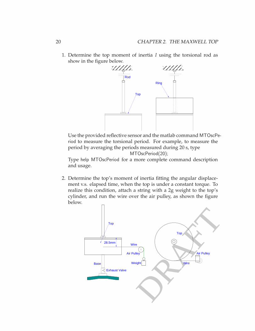
1. Determine the top moment of inertia I using the torsional rod asshow in the figure below.

Ring

Top

Rod

Use the provided reflective sensor and the matlab command MTOscPe-riod to measure the torsional period. For example, to measure theperiod by averaging the periods measured during 20 s, type

MTOscPeriod(20);Type help MTOscPeriod for a more complete command descriptionand usage.

2. Determine the top’s moment of inertia fitting the angular displace-ment v.s. elapsed time, when the top is under a constant torque. Torealize this condition, attach a string with a 2g weight to the top’scylinder, and run the wire over the air pulley, as shown the figurebelow.

Top

Base

Exhaust Valve

Weight

Air Pulley Air Pulley

Wire

Top

Wire28.5mm

DRAFT

2.5. SECOND LABORATORY WEEK 21

Adjust the exhaust valve to change the air-jets flow until the topreaches a state closest as possible to the equilibrium. Remove thestring from the top and measure the revolution periods. To keep thetorque as constant as possible, never readjust the air pressure. To ob-tain a quasi-frictionless pulley, set the air flow of the pulley in suchway the free pulley turns at very low speed. Try to keep the top asvertical as possible.Use the provided reflective sensor and the matlab command MT-CounterSave to measure the revolutions. For example, to count thetop’s revolutions for 80 s and save the time and revolutions numberinto a file called Top3Revs.Trial01.txt, type

MTCounterSave(’Top3Revs.Trial01.txt’,80);Type help MTCounterSave for a more complete command descriptionand usage.REMEMBER TO REMOVE ALL THE SCOTCH TAPE FROM THE TOP’S

RIM ONCE FINISHED.

3. Compare the two measured values of the moment of inertia I.

4. Compare the value of the angular acceleration θ0 obtained from thefit, with the value obtained from the definition of θ0 using the mo-ment of inertia I calculated in point 1.

2.5 Second Laboratory Week

The purpose of this lab is to verify that the precession angular velocity Ω

is independent of the angle φ and to study the Ω as a function of the top’scenter of mass.

If the center of the sliding mass m is placed at a distance h from thetop’s pivot, and h0 is the position of the top’s center of mass without m,the new center of mass will be located at (see Fig. 2.5)

hCM =h0M + hm

M + m(2.7)

It is important to notice that h0 is negative because it is below the pivotO, which is the origin of the reference frame chosen to compute hCM. With

DRAFT


the addition of the mass m, equation (2.4) becomes

Ω =(M + m)ghCM

Iω, (2.8)

where we have neglected the small increase in the moment of inertiaI due to the mass m. Inserting equation (2.7) into the equation (2.8), andafter some algebra, we obtain

Ω =Mg

Iωh0 +

mg

Iωh. (2.9)

which relates the precession angular velocity to the sliding mass positionh.

If we impose

h = h∗ = −h0M

m, (2.10)

the angular velocity Ω of the precession goes to zero. If the mass m isplaced at h∗, hCM is zero and the torque vanishes, and therefore the topdoes not precess.

It is important to notice that the spindle length is such that we canchange the sign of hCM.

2.5.1 Propaedeutic Problems.

1. The position of the top center of mass h0 without the sliding massm, is negative (below the pivot point). Provide a sketch depictingthe direction of the angular velocity ω and the direction of the topprecession.

2. Calculate the period of precession T for a top spinning at 5Hz (5revolutions per second, ω = 2π × 5rad/s) if m = 0.2186kg, I =4.66 · 10−2kg m2, and h = h∗ + 0.01m.

3. Given the sliding mass m = 0.2186kg with its outside diameter D =0.033m, and inside diameter d = 0.016m, calculate the sliding massmoment of inertia Im. Is the statement under equation (2.8) justified?

4. A linear fit to Ω versus h gives Ω = a + bh. What are a and b interms of m, g, I, ω and h∗? Supposing that ω is constant during

DRAFT


each measurement but different every time we change h, how can werearrange equation 2.9 to still use a straight line as fitting function ?

5. The precession period T is measured with the sliding mass removed,and for a given value of the angular velocity ω. Write the equationthat gives h0 in terms of ω, T, M, I and g.

A

BA

R B

∆2 l

6. Using two points, A and B, to align the line of sight (see figure above),a careful student determines that the uncertainty of measuring wherethe spindle passes the pointer at A is ∆l = ±2mm. If the radius ofthe precession orbit is R = 50mm, and the period is T = 60s, whatuncertainty σT does this produce in the period T? What fraction isσT of the total period T?

2.5.2 Procedure (Precession Period Measurement)

Remember to follow the directives written in section 2.3.1 (Care and Useof the Experimental Apparatus) before starting the procedure. Use thereflective sensor and the program Tachometer available form the computerdesktop to measure the revolution frequency of the top.

Setting the revolution frequency of the top at around 5Hz make thefollowing measurements:

DRAFT


1. Without the sliding mass, demonstrate that top precession period Tis independent from the angle φ for constant value of ω.

2. Using the previous measurements of the precession period T , of theangular revolution frequency ω, and of the moment of inertia I cal-culate h∗and its uncertainty . Place the sliding mass at h∗ and confirmthat the top does not precess.

3. Experimentally study the equation of the precession angular veloc-ity Ω as a function to the sliding mass position h. Be sure that youmeasure the length of the sliding mass.

4. Compare the new measurement of I obtainable from step 3 with thetwo ones of the previous week.

5. Calculate the value of h∗ obtainable from step 4 and compare it withthe previous measurement.

6. REMEMBER TO CLOSE THE AIR SUPPLY OUTPUT ONCE FINISHED.

DRAFT

Chapter 3

The Inverted Pendulum

3.1 Introduction

The purpose of this lab is to explore the dynamics of the harmonic me-chanical oscillator. To make things a bit more interesting, we will modeland study the motion of an inverted pendulum (IP), which is a special typeof tunable mechanical oscillator. As we will see below, the IP contains tworestoring forces, one positive and one negative. By adjusting the relativestrengths of these two forces, we can change the oscillation frequency ofthe pendulum over a wide range.

As usual (see section3.2), we will first make a mathematical model ofthe IP, and then you will characterize the system by measuring variousparameters in the model. Finally, you will observe the motion of the pen-dulum and see if it agrees with the model to within experimental uncer-tainties.

The IP is a fairly simple mechanical device, so you should be able toanalyze and characterize the system almost completely. At the same time,the inverted pendulum exhibits some interesting dynamics, and it demon-strates several important principles in physics. Waves and oscillators areeverywhere in physics and engineering, and one of the best ways to un-derstand oscillatory phenomenon is to carefully analyze a relatively sim-ple system like the inverted pendulum.

25

DRAFT

26 CHAPTER 3. THE INVERTED PENDULUM

3.2 Modeling the Inverted Pendulum (IP)

3.2.1 The Simple Harmonic Oscillator

We begin our discussion with the most basic harmonic oscillator – a massconnected to an ideal spring. We can write the restoring force F = −kx inthis case, where k is the spring constant. Combining this with Newton’slaw, F = ma = mx, gives x = −(k/m)x, or

x + ω20x = 0 (3.1)

with ω20 = k/m

The general solution to this equation is x(t) = A1 cos(ω0t)+ A2 sin(ω0t),where A1 and A2 are constants. (You can plug x(t) in yourself to see thatit solves the equation.) Once we specify the initial conditions x(0) andx(0), we can then calculate the constants A1 and A2. Alternatively, we canwrite the general solution as x(t) = A cos(ω0t + ϕ), where A and ϕ areconstants.

The math is simpler if we use a complex function x(t) in the equation,in which case the solution becomes x(t) = Aeiω0t, where now A is a com-plex constant. (Again, see that this solves the equation.) To get the actualmotion of the oscillator, we then can take the real part (or the imaginarypart), so x(t) = Re[x(t)]1

You should be aware that physicists and engineers have become quitecavalier with this complex notation. We often write that the harmonic os-cillator has the solution x(t) = Aeiω0t without specifying what is complexand what is real. This is lazy shorthand, and it makes sense once youbecome more familiar with the dynamics of simple harmonic motion.

The Bottom Line: Equation 3.1 gives the equation of motion for a sim-ple harmonic oscillator. The easiest way to solve this equation is using thecomplex notation, giving the solution x(t) = Aeiω0t.

3.2.2 The Simple Pendulum

The next step in our analysis is to look at a simple pendulum. Assumea mass m at the end of a massless string of a string of length ℓ. Gravity

1If you have not yet covered why this works in your other courses, see the EndNoteat the end of this chapter.

DRAFT

3.2. MODELING THE INVERTED PENDULUM (IP) 27

exerts a force mg downward on the mass. We can write this force as thevector sum of two forces: a force mg cos θ parallel to the string and a forcemg sin θ perpendicular to the string, where θ is the pendulum angle. (Youshould draw a picture and see for yourself that this is correct.) The forcealong the string is exactly countered by the tension in the string, while theperpendicular force gives us the equation of motion

Fperp = −mg sin θ (3.2)

= mℓθ

so θ + (g/ℓ) sin θ = 0

As it stands, this equation has no simple analytic solution. However wecan use sin θ ≈ θ for small θ, which gives the harmonic oscillator equation

θ + ω20θ = 0 (3.3)

where ω20 = g/ℓ (3.4)

The Bottom Line: A pendulum exhibits simple harmonic motion de-scribed by Equation 3.3, but only in the limit of small angles.

3.2.3 The Simple Inverted Pendulum

Our model for the inverted pendulum is shown in Figure 3.1. Assumingfor the moment that the pendulum leg has zero mass, then gravity exertsa force

Fperp = +Mg sin θ (3.5)

≈ Mgθ

where Fperp is the component of the gravitational force perpendicular tothe leg, and M is the mass at the end of the leg. The force is positive,so gravity tends to make the inverted pendulum tip over, as you wouldexpect.

In addition to gravity, we also have a flex joint at the bottom of the legthat is essentially a spring that tries to keep the pendulum upright. Theforce from this spring is given by Hooke’s law, which we can write

Fspring = −kx (3.6)

= −kℓθ

DRAFT


Leg

Flex Joint

l

Mass

θM θ

Mgkl

θ

Mg

Figure 3.1: Simple Inverted Pendulum.

where ℓ is the length of the leg.The equation of motion for the mass M is then

Mx = Fperp + Fspring (3.7)

Mℓθ = Mgθ − kℓθ

and rearranging gives

θ + ω20θ = 0 (3.8)

where ω20 =

k

M− g

ℓ(3.9)

If ω20 is positive, then the inverted pendulum exhibits simple harmonic

motion θ(t) = Aeiω0t. If ω20 is negative (for example, if the spring is too

weak, or the top mass is to great), then the pendulum simply falls over.The Bottom Line: A simple inverted pendulum (IP) exhibits simple

harmonic motion described by Equation 3.8. The restoring force is sup-plied by a spring at the bottom of the IP, and there is also a negative restor-ing force from gravity. The resonant frequency can be tuned by changingthe mass M on top of the pendulum.

DRAFT

3.2. MODELING THE INVERTED PENDULUM (IP) 29

3.2.4 A Better Model of the Inverted Pendulum

The simple model above is unfortunately not good enough to describe thereal inverted pendulum in the lab. We need to include a nonzero massm for the leg. In this case it is best to start with Newton’s law in angularcoordinates

Itotθ = τtot (3.10)

where I is the total moment of inertia of the pendulum about the pivotpoint and τ is the sum of all the relevant torques. The moment of inertiaof the large mass is IM = Mℓ2, while the moment of inertia of a thin rodpivoting about one end (you can look it up, or calculate it) is Ileg = mℓ2/3.Thus

Itot = Mℓ2 +

mℓ2

3(3.11)

=(

M +m

3

)

ℓ2

The torque consists of three components

τtot = τM + τleg + τspring (3.12)

= Mgℓ sin θ + mg

(

ℓ

2

)

sin θ − kℓ2θ

The first term comes from the usual expression for torque τ = r× F, whereF is the gravitational force on the mass M, and r is the distance betweenthe mass and the pivot point. The second term is similar, using r = ℓ/2for the center-of-mass of the leg. The last term derives from Fspring = −kℓθabove, converted to give a torque about the pivot point.

Using sin θ ≈ θ, this becomes

τtot ≈ Mgℓθ + mg

(

ℓ

2

)

θ − kℓ2θ (3.13)

≈[

Mgℓ+mgℓ

2− kℓ2

]

θ

and the equation of motion becomes

Itotθ = τtot (3.14)(

M +m

3

)

ℓ2θ =

[

Mgℓ+mgℓ

2− kℓ2

]

θ (3.15)

DRAFT


which is a simple harmonic oscillator with

ω20 =

kℓ2 − Mgℓ− mgℓ2

(

M + m3

)

ℓ2(3.16)

This expression gives us an oscillation frequency that better describesour real inverted pendulum. If we let m = 0, you can see that this becomes

ω20(m = 0) =

k

M− g

ℓ(3.17)

which is the angular frequency of the simple inverted pendulum describedin the previous section. If we remove the top mass entirely, so that M = 0,you can verify that

ω20(M = 0) =

3k

m− 3g

2ℓ(3.18)

The Bottom Line: The math gets a bit more complicated when the legmass m is not negligible. The resonance frequency of the IP is then givenby Equation 3.16. This reduces to Equation 3.17 when m = 0, and to Equa-tion 3.18 when M = 0.

3.3 The Damped Harmonic Oscillator

To describe our real pendulum in the lab, we will have to include dampingin the equation of motion. The major source of damping comes from theflex joint which is unable to give all the energy back during its bendingmotion. One way to account for this, is to use a complex spring constantgiven by

k = k(1 + iφ) (3.19)

where k is the normal (real) spring constant and φ (also real) is called theloss angle. Looking at a simple harmonic oscillator, the equation of motionbecomes

mx = −k(1 + iφ)x (3.20)

which we can write

x + ω2dampedx = 0 (3.21)

with ω2damped =

k(1 + iφ)

m(3.22)

DRAFT

3.4. THE DRIVEN HARMONIC OSCILLATOR 31

If the loss angle is small, φ ≪ 1, we can do a Taylor expansion to get theapproximation

ωdamped =

√

k

m(1 + iφ)1/2 (3.23)

≈√

k

m(1 + i

φ

2) (3.24)

= ω0 + iα (3.25)

with α =φω0

2(3.26)

Putting all this together, the motion of a weakly damped harmonic os-cillator becomes

x(t) = Ae−αteiωot (3.27)

which here A is a complex constant. If we take the real part, this becomes

x(t) = Ae−αt cos(ω0t + ϕ) (3.28)

This is the normal harmonic oscillator solution, but now we have the extrae−αt term that describes the exponential decay of the motion.

We often refer to the quality factor Q of an oscillator, which is defined as

Q = ωEnergy stored

Power loss(3.29)

Note that Q is a dimensionless number. For our case this becomes (thederivation is left for the reader)

Q ≈ ω0

2α=

1

φ(3.30)

The Bottom Line: We can model damping in a harmonic oscillator byintroducing a complex spring constant. Solving the equation of motionthen gives damped oscillations, given by Equations 3.27 and 3.28 whenthe damping is weak.

3.4 The Driven Harmonic Oscillator

If we drive a simple harmonic oscillator with an external oscillatory forceF0eiωt, then the equation of motion becomes

x + ω2dampedx =

F0

meiωt (3.31)

DRAFT


where ω is the angular frequency of the drive force and F0 is the forceamplitude. (As above, ωdamped = ω0 + iα.) Analyzing this shows that thesystem first exhibits a transient behavior that lasts a time of order

ttransient ≈ α−1 ≈ 2Q/ω0 (3.32)

During this time, the motion is quite complicated and depends on the ini-tial conditions and the phase of the applied force.

Because of the damping, the transient behavior eventually dies away,however, and for t ≫ ttransient the system settles into a steady-state behav-ior, where the motion is given by

x(t) = Xeiωt (3.33)

In other words, in steady-state the system oscillates with the same fre-quency as the applied force, regardless of the natural angular frequencyω0. Plugging this x(t) into the equation of motion quickly gives us

X =F0/m

ω2damped − ω2

(3.34)

Since X is a complex constant, it gives the amplitude |X| and phasearg (X) of the motion. When the damping is small (α ≪ ω0), we can writeω2

damped ≈ ω20 + 2iαω0, giving

X ≈ F0/m(

ω20 − ω2

)

+ 2iαω0(3.35)

and the amplitude of the driven oscillations becomes

|X (ω)| = F0/m√

(

ω20 − ω2

)2+ 4α2ω2

0

(3.36)

Note that the driven oscillations have the highest amplitude on resonance(ω = ω0), and the peak amplitude is highest when the damping is lowest.

The Bottom Line: Once the transient motions have died away, a har-monically driven oscillator settles into a steady-state motion exhibitingoscillation at the same frequency as the drive. The amplitude is higheston resonance (when ω = ω0) and when the damping is weak, as given byEquation 3.36.

DRAFT

3.5. THE TRANSFER FUNCTION 33

3.5 The Transfer Function

For part of this lab you will shake the base of the inverted pendulum andobserve the response. To examine this theoretically, we can look first atthe simpler case of a normal pendulum in the small-angle approximation(when doing theory, always start with the simplest case and work up). Theforce on the pendulum bob (see Equation 3.2) can be written

F = −mgx/ℓ (3.37)

where x is the horizontal position of the pendulum and ℓ is the length.If we shake the top support of the pendulum with a sinusoidal motion,xtop = Xdriveeiωt, then this becomes

F = −mg(

x − xtop

)

/ℓ (3.38)

x + ω20x = ω2

0xtop (3.39)

where ω20 = g/ℓ. With damping this becomes

x + ω2dampedx = ω2

0xtop (3.40)

= ω20Xdriveeiωt (3.41)

which is essentially the same as Equation 3.31 for a driven harmonic oscil-lator. From the discussion above, we know that this equation has a steady-state solution with x = Xeiωt. It is customary to define the transfer function

H(ω) =X

Xdrive(3.42)

which in this case is the ratio of the motion of the pendulum bob to themotion of the top support. Since H is complex, it gives the ratio of theamplitudes of the motions and their relative phase.

For the simple pendulum case, Equation 3.35 gives us (verify this foryourself)

H(ω) ≈ ω20

(

ω20 − ω2

)

+ 2iαω0(3.43)

At low frequencies (ω ≪ ω0) and small damping (α ≪ ω0), this becomesH ≈ 1, as you would expect (to see this, consider a mass on a string,

DRAFT


and shake the string as you hold it in your hand). At high frequencies(ω ≫ ω0), this becomes H(ω) ≈ −ω2

0/ω2, so the motion of the bob is 180degrees out of phase with the motion of the top support (try it).

The Bottom Line: The transfer function gives the complex ratio of twomotions, and it is often used to characterize the behavior of a driven os-cillator. Equation 3.43 shows one example for a simple pendulum. Themotion of the inverted pendulum is a bit more interesting, as you will seewhen you measure H(ω) in the lab.

3.6 The Inverted Pendulum Test Bench

3.6.1 Care and Use of the Apparatus

The Inverted Pendulum hardware is not indestructible, so please treat itwith respect. Ask your instructor if you think something is broken or oth-erwise amiss. The flex joint is particularly delicate, and bending it to largeangles can cause irreparable damage. Follow these precautions:

1. NEVER LET THE IP OSCILLATE WITHOUT THE TRAVEL LIMITER.

2. DO NOT LET THE IP LEG FALL.

3. DO NOT DISASSEMBLE THE IP WITHOUT ASSISTANCE FROM YOUR

INSTRUCTOR.

3.7 The Lab - First Week

3.7.1 Pre-Lab Problems

1. Rewrite Equation 3.16 using the “rotational stiffness” variable κ = kℓ2

for the spring constant. What are the units of k, κ?

2. Determine the length of an IP leg with a load of M = 0.383 kg, flex jointrotational stiffness κ = 2.5 Nm/rad, oscillation period T = 10 seconds,and negligible leg mass, m = 0. Compute the length of a simple pendulum

with the same oscillation frequency. Assume g = 9.81 m/s2.

3. For the IP in Problem 2, calculate the mass difference ∆M needed tochange the period from 10 seconds to 100 seconds. At what mass M∗doesthe period go to infinity?

DRAFT

3.7. THE LAB - FIRST WEEK 35

VelocitySensor

VelocitySensor

ShakerTable

DamperPlate

LevelingScrew

Actuator Platform

Leg

ActuatorShim Stock

Disks

Flex Joint Base

Travel Limiter

Connector

Coil

Permanent Magnet

Figure 3.2: Inverted pendulum test bench .

4. For the IP in Problem 2, if the loss angle is φ = 10−2, how long does ittake for the motion to damp down to 1% of its starting amplitude?

3.7.2 In-Lab Exercises

3.7.2.1 Getting Started

Please read down to the end of this section before beginning your work.Once you begin in the lab, record all your data and other notes in yournotebook as you proceed. Print out relevant graphs and tape them intoyour notebook as well.

DRAFT


Step 1. All the measurements this week are done with the actuator plat-form locked in place. Use the attached thumb screws to lock the platform(see your instructor if you are not sure about this). If the platform is se-curely locked, it should not rattle if you shake it gently.

Load device

l

Arrow shaftFlex joint

Figure 3.3: IP leg with the flex joint and the load device.

3.7.2.2 The IP Leg

When adding mass to the top of the leg, add weights symmetrically onthe load device (see Figure 3.3). This ensures that the center-of-mass ofthe added weight is always positioned at the same distance from the pivotpoint (i.e., this ensures that ℓ stays constant as you change M).

Step 2. Using the spare leg in the lab, measure the length ℓ and massm of the leg, including measurement uncertainties (error bars). Measure ℓ

from the center of the flex joint to the center-of-mass of the added weight.Note that you cannot actually measure ℓ very well because of the largesize of the flex joint. Use common sense to estimate an uncertainty in ℓ,based on the length of the flex joint and how accurately the load mass canbe placed. Note that your measurement of m does not include the massof the magnet assembly on the IP, which you can take to be Mmagent = 6grams.

3.7.2.3 Resonant Frequency versus Load

Step 3. With no mass on the top of the leg (M = 0), measure the oscillationperiod P = 1/2πω1 (with an error bar) of the IP using the Matlab data-acquisition function IPRingDown. Use Equation 3.16 to estimate k based

DRAFT

3.7. THE LAB - FIRST WEEK 37

on your frequency measurement. Use your direct measurements of m andℓ. Assuming that the theory in Equation 3.16 is exact, use standard errorpropagation methods to estimate an error bar for k from the errors in theother quantities.

Step 4. Make additional measurements of P for different values of Mstarting with the largest mass you will plan to use. Add washers sym-metrically about the center-of-mass (see Figure 3.3). Note that you mayhave to level the IP as you add more mass using the three leveling thumbscrews; ask your instructor if you need help. As the top mass M increases,the IP is more likely to tip over, so the leveling of the apparatus is quiteimportant.

For each measurement of P, measure M using the scale in the lab. Takeat least 5-7 data points with error bars. Note that the errors in the mea-surement of P are larger for larger P.

Step 5. Use Equation 3.16 to compute a theoretical curve to add toyour data plot. One way to accomplish this is by creating a short Matlabprogram (a ”.m file” or script file). Here is an example (ask your instructorif you need help on how to edit and save your own program in Matlab):

DRAFT


% Dec 2, 2012

% IP PeriodVersusMass.m

% Sample program to plot IP data with theory

% replace ? with values%

clear; %clear all variables

%% Measurements

m = ?; % kg, measured shaft mass

l = ?; % m, measured shaft length

M Magnet = 0.010; % kg, extra mass from magnet assembly

M measured = [? ? ? ? ? ]+M Magnet; % kg, measured added mass

T measured = [? ? ? ? ? ]; % s, measured period

%% Constants

g = 9.81; % m/sˆ2, gravitational constant

%%Guess for k

k = input(’Enter educated guess for k: ’);

%% Compute the theoretical curve

M = 0.01:.001:0.35; %kg, mass vector for theoretical curve

w0 = sqrt( ( k*lˆ2 - M*g*l - m*g*l/2 ) ./ ((M + m/3)*lˆ2) ); % rad/s

T = 2*pi./w0; %s, theoretical oscillation period

close all; % close all figures

%% Plot Theoretical data in semilog scale

semilogy(M,T,’b’)

hold(’on’) %hold the current so new plot can be added

%% Plot experimental data

plot(M measured,T measured,’o’)

xlabel(’Added mass M, [kg]’)

ylabel(’IP period T , [s]’)

axis(’tight’)

grid(’on’)

hold(’off’)

Try putting in different values of k to see how the theory changes. Youshould get a nice fit using your calculated value of k, although a differ-ent value may fit better. The real IP is not exactly the same as depicted in

DRAFT

3.8. THE LAB - SECOND WEEK 39

theory, so there will be some systematic discrepancies, and some parame-ter estimation (IP length for example) can have systematic errors. Plot thedata with theory for your best subjective estimate of k, and add the plot toyour notebook.

Step 6. Create a difference plot of your experimental data points andthe theoretical curve to re-estimate k ( hint: copy and modify the Matlabprogram you already wrote and use the PlotBoxesLinLin command to plotyour experimental data points.)

Step 7. From observing how well the theory fits the data for differentguesses for k, estimate your best-fit k along with an error bar (hint: use thedifference plot). How does this compare with your estimate of k in Step 6and 3?

3.8 The Lab - Second Week

3.8.1 Pre-Lab Problems

1. Using matlab or your prefered tool, plot the amplitude response of adriven harmonic oscillator, given by Equation 3.36. Assume a resonancefrequency ω0 = 2π Hz, F0/m = 1, and plot the amplitude as a function ofangular frequency ω . Make three plots (preferably all on a single graph)using Q = 1, 10, and 100. Plot all three on a linear-linear plot, then plot allthree again on a log-log plot. Note that the response shows a power-lawbehavior (x ∼ ω−2) at high frequencies, and this appears as a straight linein the log-log plots. Consult the matlab plot script examples posted on theph3 web pages.

2. Let ∆ω be the FWHM (full-width at half-maximum) width of |A(ω)|2,

i.e. when ω = ω0 ± ∆ω/2, then |A (ω0 ± ∆ω/2)|2 = |A (ω0)|2 /2. In thelimit of high Q, find Q as function of ω0 and ∆ω. (Hint: use Equation 3.36

and find an approximate formula for |A (ω)|2 by imposing ω = ω0 + ε,and neglecting terms of the order ε3 and higher .

3. In the lab we will measure X(ν) and Xdrive(ν), the velocities of thependulum bob and support platform. Show that H(ν) = X(ν)/Xdrive(ν) =X(ν)/Xdrive(ν).

DRAFT


3.8.2 In-Lab Exercises

3.8.2.1 Inverted Pendulum Loss Angle

Step 1. With the actuator platform locked (same as last week), use IPRing-Down to observe the motion of the inverted pendulum with no addedmass and no added damping. Put a plot of the IP motion xIP(t) in yournotebook, and estimate the loss angle φ from the time it takes the motionto damp away. Now add the aluminum damper plate to the top of theIP assembly (ask your instructor). As the pendulum swings, the dampingmagnet induces a current in the aluminum plate, which heats the plateand extracts energy from the IP motion. With the aluminum plate in place(about 6 mm from the magnet), again plot xIP(t) and estimate φ from afit. Unscrew the magnet holder tube a bit so the magnet is quite close tothe plate, and again plot xIP(t) and estimate φ. For each case, how long isttransient – the time needed for a driven system to reach steady-state motion(see Equation 3.32)?

3.8.2.2 The Transfer Function

The rest of the lab is done with the actuator platform unlocked; ask yourinstructor if you need help with this. Drive the motion of the platformusing a sinusoidal voltage from the signal generator. Be sure to set the”sweep” button to EXT (which turns off the sweep feature of the signalgenerator). With a high signal amplitude you should be able to see theplatform oscillating, and you can see the frequency change as you changethe frequency of the drive voltage. MAKE SURE THAT THE MOTION OF THE

PLATFORM IS SINUSOIDAL.With no added mass on the IP, use the Matlab program IPTransmissibility

to measure the motion of the platform xplat f orm(t) and the motion of thetop mass xIP(t). Use the ’t’ command to view both motions as a functionof time. If both do not show simple sinusoidal oscillations, turn down thedrive amplitude. The program IPTransmissibility will collect data for you asyou change the drive frequency, and it will compare xIP(t) and xplat f orm(t)to give you the amplitude and phase of the transfer function as a functionof frequency.

Step 2. Collect data at a sufficient number of drive frequencies to mapout the transfer function H(ν) as a function of frequency. Put a plot ofH(ν) in your notebook, and qualitatively explain the features of H(ν)

DRAFT

3.9. ENDNOTE: USING COMPLEX FUNCTIONS TO SOLVE REAL EQUATIONS41

(both amplitude and phase), given the above discussion of a driven har-monic oscillator.

Step 3. Now add mass to the IP so the resonant frequency is between0.5 and 1 Hz (use your data from last week to see what M is needed). Placethe damper plate about 3 mm from the damping magnet. Starting at lowfrequencies, use IPTransmissibility to again map out H(ν). Again, use the’t’ command to make sure the motions are sinusoidal. Above the reso-nance frequency of the IP, you will need to turn up the drive amplitudeso the signal-to-noise in the measurements remains adequate. Be sure tocontinue your measurements to at least 10 Hz. Put a plot of H(ν) in yournotebook, and again qualitatively explain the features of H(ν) (both am-plitude and phase). [Hint: an understanding of the ”center of percussion”of a bar will be useful for explaining the high-frequency behavior.]

3.9 EndNote: Using Complex Functions to Solve

Real Equations

Physicists and engineers often use complex functions to solve real equa-tions, with the understanding that you take the real part at the end. Whydoes this work? And why do we even do this? We can demonstratewith the simple harmonic oscillator. Start with the equation of motionx + ω2

0x = 0, and let us solve this using a complex function: x = α + iβ,where α(t) and β(t) are real functions. If you plug this in, you will see thatx + ω2

0x = 0 becomes

(

α + iβ)

+ ω20 (α + iβ) = 0 (3.44)

(

α + ω20α)

+ i(

β + ω20β)

= 0

Since a complex number equals zero only if both the real and imaginaryparts equal zero, we see that x + ω2

0x = 0 implies that both α + ω20α = 0

and β+ ω20β = 0. In other words, both the real and imaginary parts of x(t)

satisfy the original equation.So we have a procedure: try using a complex function to solve the

original equation. If this works, then taking the real part of the solutiongives a real function that also solves the same differential equation. (If indoubt, then verify directly that the real part solves the equation.)

DRAFT


Why do we go to the trouble of using complex functions to solve a realequation? Because differential equations are often easier to solve when weassume complex functions (it seems counter-intuitive, but it’s true). Thefunction eiω0t is a simple exponential, and the derivative of an exponentialis another exponential – that makes things simple. In contrast, cosines andsines are more difficult to work with.

In the case of the simple harmonic oscillator, the solution x(t) = Aeiωt

has a natural interpretation. The length and angle of the A vector (in thecomplex plane) give the amplitude and phase of the oscillations.

You should note, however, that this only works for linear equations. Ifour equation were x + ω2

0x + γx2 = 0, for example, then using complexfunctions would not have the same benefits. In fact there is no simple so-lution to this equation, complex or otherwise. This equation describes anonlinear oscillator, and nonlinear oscillators exhibit a fascinating dynam-ics with interesting behaviors that people still study to this day.

DRAFT

Chapter 4

Direct Current Network Theory

4.1 Electronic Networks

An electronic network or circuit is a set of electronic components/devicesconnected together to modify and transmit/transfer energy/information.This information is generally called electric signal or simply signal. Tographically represent a network, we use a set of coded symbols with termi-nals for devices and lines for connections. These lines propagate the signalamong the devices without changing it. Devices change the propagationof the electric signals instead.

Quantities defining this propagation are the voltages V across the de-vices and currents I flowing through them.

Solving an electronic network means determine the currents or thevoltages on each point of it.

To make the understanding of network basic theorems easier, somemore or less intuitive definitions must be stated.

4.1.1 Network Definitions

A network node is a point where more than two network lines connect.A network loop, or mesh, is any closed network line. To determine a mesh

it is sufficient to start from any point of the circuit and come back runningthrough the network to the same point without passing through a samepoint.

Figure 4.1 shows a generic portion of a network with 4 visible nodes,

43

DRAFT

44 CHAPTER 4. DIRECT CURRENT NETWORK THEORY

Figure 4.1: Generic representation of a network

and 3 visible meshes. The empty boxes are the electronic components ofthe network. The electronic components are points of the network.

4.1.2 Series and Parallel

Let’s consider the two different connection topologies shown in figure 4.2,the parallel and the series connections.

A set of components is said to be in series if the current flowing throughthem and anywhere in the circuit is the same .

A set of components is said to be in parallel if the voltage differencebetween them is the same.

B

A

A B

Figure 4.2: Considering the points A, and B, the components of the leftcircuit are in parallel, and those ones in the right circuit are in series.

DRAFT

4.2. KIRCHHOFF’S LAWS 45

A B

I

R

V

Figure 4.3: Resistor symbol

4.1.3 Active and Passive Components

Circuit components can be divided into two categories: active and passivecomponents. Active components are those devices that feed energy intothe network. Voltage and current sources are active components. Ampli-fiers are also considered active components.

Passive components are those components that do not feed energy tothe network. Resistors, capacitors, inductors are typical passive compo-nents.

In general, both active and passive components dissipate energy.

4.2 Kirchhoff’s Laws

In this section the two Kirchhoff’s laws, which are fundamental for thesolution of an electronic circuit are stated here.Kirchhoff’s Voltage Law (KVL):The algebraic sum of the voltage differ-ence vk around a mesh must be equal to zero at all times, i.e.

∑k

v(t) = 0

Kirchhoff’s Current Law(KCL):The algebraic sum of the currents ik enter-ing and leaving a node must be equal to zero at all times, i.e.

∑k

ik(t) = 0.

4.3 Resistors (Ohm’s Law)

It is experimentally known that if we apply a voltage V across a metal (aconductor), we will measure an electric current I flowing through it. V

DRAFT


results to be proportional to I by a constant R, named electric resistance ofthe conductor. In other terms we have

V

I= R, (4.1)

which is called Ohm’s law. The unit for the resistance is the “Ohm” whosesymbol is the Greek letter Ω. It follows from Ohm’s law that [Ω] = [V/A]=“Voltper Ampere”.

In a metallic conductor, R is proportional to the conductor length l andinversely proportional to the cross-section s, i.e.

R = ρl

s.

ρ is the conductor resistivity and it depends on the metal and its impu-rities. A device which follows Ohm’s Law is said to be a resistor and itssymbol is shown in figure 4.3.

The power P dissipated by the resistor with resistance R is

P = VI, ⇒ P =V2

R= RI2.

Let’s define some properties of the resistance of conductors.

4.3.1 Resistors in Series

R1 R2

V1 V2 Vn

Vtot

Rtot

I I I

Rn

Figure 4.4: Resistor in series

The resistance Rtot of a set of resistor R1,R2, . . . , Rn, connected in series(see figure 4.4), is equal to the sum of the resistances

DRAFT

4.3. RESISTORS (OHM’S LAW) 47

Rtot =n

∑k=1

Rk.

The previous formula is easy to demonstrate. Connecting the resistorseries to a voltage source V, and applying the (4.1) to each resistors wehave

V1 = R1 I, V2 = R2 I, ... Vn = Rn I,

where I is the current flowing through each resistor. Because of the KVL,the voltage difference V must be the sum of all the voltages differences,i.e.

V =n

∑k=1

Rk I =

(

n

∑k=1

Rk

)

I.

4.3.2 Resistors in Parallel

The inverse of the resistance Rtot of a set of resistor R1,R2, . . . , Rn, con-nected in parallel (see figure 4.5), is equal to the sum of the inverse of theresistances

1

Rtot=

n

∑k=1

1

Rk.

This law can be easily derived using (4.1) and the definition of compo-nents in parallel.

V RnR1 R2 Rtot1 2 nI I I

totI

Figure 4.5: Resistors in parallel.

DRAFT


A B

I

V

C

Figure 4.6: Capacitor symbol.

4.4 Capacitors

Let’s study another typical component of an electronic circuit, the capac-itor. A capacitor is a system of two conductors which goes under fullinduction when a voltage difference is applied to the conductors. Eachconductor will be charged with the same amount of charge Q with op-posite sign. The ratio between the voltage difference V between the twoconductors and the charge Q

C =Q

V(4.2)

is constant and is said to be the capacitance C of the capacitor. The capac-itance depends on the geometry of the conductors and on the interposeddielectric. The units for the capacitance is the “Faraday” whose symbol isthe letter F. It follows that [F] = [C/V]=“Coulomb per Volt”.

4.4.1 Capacitors in Parallel

A parallel of capacitors C1, C2, ..., Cn is a capacitor whose capacitance Ctot

is the sum of all the capacitances, i.e.

Ctot =n

∑k=1

Ck. (4.3)

The previous formula is easy to demonstrate. In fact, the total inducedcharge Qtot on the capacitors side at the same potential is equal to the sumof all charges of those sides, i.e.

Qtot =n

∑k=1

Qk.

Considering that the voltage difference V across each capacitor must besame, and dividing by V we obtain the (4.3).

DRAFT

4.4. CAPACITORS 49

V C1 C2 totnC C

Figure 4.7: Capacitors in parallel.

4.4.2 Capacitors in Series

A series of capacitors C1, C2, ..., Cnis a capacitor with capacitance Ctot sat-isfying the following equation

1

Ctot=

n

∑k=1

1

Ck.

The demonstration of the previous equation is left as exercise (hint: inthis case the induced charges are equal and not the voltage differencesacross the capacitors).

V1 V2 Vn

Vtot

C2C1

Ctot

Cn

Figure 4.8: Capacitors in series.

DRAFT


4.5 Ideal and Real Sources

4.5.1 Ideal Voltage Source

An ideal voltage source is a source able to deliver a given Voltage differ-ence Vs between its leads independently of the load R attached to it (seefigure 4.9). It follows from Ohm’s law that a voltage source is able to pro-duce any current I to keep constant the voltage difference Vs across theload R. The symbol for the ideal voltage source is shown in figure 4.9.

Quite often, a real voltage source exhibits a linear dependency on theresistive load R. It can be represented using an ideal voltage source Vs inseries with a resistor Rs called input resistance of the source. ApplyingOhm’s law, it can be easily shown that the voltage and current throughthe load R are

V =R

R + RsVs, I =

Vs

R + Rs.

If we assume

R ≫ Rs, ⇒ V ≃ Vs, I ≃ Vs

R.

Under the previous condition, the real voltage source approximates theideal case.

sV sV

+

−

VRI

V

I

Figure 4.9: Ideal voltage source.

4.5.2 Ideal Current Source

An ideal current source is a source able to deliver a given current Is whichdoes not depend on the load R attached to it (see figure 4.10). It followsfrom Ohm’s law that an ideal current source is able to produce any voltage

DRAFT

4.6. THE SEMICONDUCTOR JUNCTION (DIODE) 51

difference V across the load R to keep Is constant. The symbol for the idealcurrent source is shown in figure 4.10.

A real current source exhibits a dependency on the resistive load R,which can be represented using an ideal current source Is in parallel witha resistor Rs. Applying Ohm’s law and the KCL, it can be easily shownthat the voltage and current through the load R are

I =Rs

R + RsIs, V =

RsR

Rs + RIs.

If we suppose

Rs ≫ R, ⇒ I ≃ Is, V ≃ RIs ≫ 0

Under the previous condition, the real current source approximates theideal case.

sVIs

Is

VRI

V

I

Figure 4.10: Ideal current source.

4.6 The Semiconductor Junction (Diode)

The semiconductor junction or semiconductor diode is a device which presentsa non-linear behavior due to its peculiar conduction mechanism substan-tially different from the conduction in a metal.

If ID and VD are the current and the voltage difference across the junc-tion, we will have

ID(VD) = I0(e−qVDηkBT − 1), (4.4)

where kB = 1.3807 · 10−23J/K is the Boltzmann constant, T the absolutetemperature, q = −1.60219 · 10−19C the electron charge, and η a dimen-sionless parameter, which depends on the diode type. I0 is the reversesaturation current.

DRAFT


Instead of following Ohm’s law, the semiconductor junction follows anexponential curve (the diode I-V Characteristic). Deviations from this laware negligible depending on the current magnitude and the diode charac-teristics.

Figure 4.11 shows the standard symbol for a semiconductor diode andthe I-V characteristic. The break-down voltage Vb reported in the samefigure is the reverse voltage which essentially shorts circuit the junction.This behavior is not accounted by the equation (4.4).

Vb

Von

ID

I0DV

DV

A

B

ID

0

Figure 4.11: Diode characteristic (continuous curve), simplified diodecharacteristic (dashed curve), and diode standard symbol.

A simplified model of the junction diode is that one of a perfect switch,i.e.

ID(V) =

∞ V ≥ Von

0 V < Von,

where Von is the diode turn-on voltage, which depends on the junction typeand on the current magnitude. For current up to ID ∼ 100mA, silicondiodes have Von ≃ 0.6V, and germanium diodes have Von ≃ 0.3V .

For voltages greater than Von, the diode is a short circuit (current is notlimited by the diode) and is said to be forward biased. For smaller values itis an open circuit (current across the diode is zero ) and is reverse biased.

DRAFT

4.7. EQUIVALENT NETWORKS 53

ComplexCircuit

ComplexCircuit

V2

VTot

R1

R2

V2

VTot

I

A

B

C

A

B

C

Figure 4.12: Simplest and complex voltage divider circuit.

4.7 Equivalent Networks

Quite often, the analysis of a network becomes easier by replacing part ofit with an equivalent and simpler network or dividing it into simpler sub-networks. For example, the voltage divider is an equation easy to remem-ber that allows to divide a complex circuit in two parts simplifying thesearch of the solution. Thevenin and Norton theorems, give us two meth-ods to calculate equivalent simple circuits, which behave like the originalcircuit seen from two points of it. These techniques briefly explained inthis section, will be used also in some of the next experiments.

4.7.1 Voltage Divider

The voltage divider equation is applicable every time we have a circuitwhich can be re-conducted in a series of two simple or complex compo-nents. The simplest case is the one shown in figure 4.12. Applying Ohm’slaw, we have

VTot = (R1 + R2)I

V2 = R2 I

and indeed

V2 =R2

R1 + R2VTot,

which is the equation of the voltage divider. The equation still holds if wereplace the resistance seen from the points A, B for R1and B,C for R2.

DRAFT


4.7.2 Thevenin Theorem

Thevenin theorem allows to find an equivalent circuit of a network seenfrom two points A and B using the series of an ideal voltage source ofvoltage VTh and a resistor with resistance RTh.

RL RLV

R

Th

Th

Black Box

+

−

B

A

B

A

Figure 4.13: Thevenin equivalent circuit illustration.

The equivalence means that if we place a load RL between A and Bin the original circuit (see figure 4.13) and measure the voltage VL and thecurrent IL across the load, we will obtain exactly the same VL and IL if RLisplaced in the equivalent circuit. This must be true for any load we connectto the points A and B .

The previous statement and the linearity of the circuit can be used tofind VTh and RTh. In fact, if we consider RL = ∞ (open circuit, OC), wewill have

VTh = VOC .

The Voltage VTh is just the voltage difference between the two leads Aand B.

For RL = 0 (short circuit, SC) we must have

ISC =VTh

RTh=

VOC

RTh.

and therefore

RTh =VOC

ISC.

The last expression says that the Thevenin resistance is the resistanceseen from the points A and B of the original circuit.

If the circuit is known the Thevenin parameter can be calculated inthe case of the terminals A and B open. In fact, VTh is just the voltage

DRAFT

4.7. EQUIVALENT NETWORKS 55

Vs+

−V0

R1

RTh

VTh

R2

R0R0

V0

+

−

A

B

A

B

+

−+

−

Figure 4.14: Thevenin equivalent circuit example

across A and B of a known circuit. Replacing the ideal voltage sourceswith short circuits (their resistance is zero) and ideal current sources withopen circuits ( their resistance is infinite) we can calculate the resistanceRTh seen from terminals A and B.

Example:

We want to find the Thevenin circuit of the network enclosed into the grayrectangle of figure 4.14. To find RTh, and VTh we have to disconnect thecircuit in the points A and B. In this case voltage difference between thesetwo points, thanks to the voltage divider equation, is

VTh =R1

R1 + R2Vs.

Short circuiting Vs we will have R1 in parallel with R2. The Theveninresistance RTh will be indeed

RTh =R1R2

R1 + R2.

Considering the previous results, we can finally state Thevenin theo-rem as follows:

Any circuit seen from two points can be replaced by a series of an ideal voltagesource of voltage VTh and a resistor of resistance RTh. VTh is the voltage difference

DRAFT


between the two point of the original circuit. RTh is the resistance seen from thesetwo points, short-circuiting all the ideal voltages generators and open-circuitingall the ideal current generators.

RLRNoBlack Box RL I No

Figure 4.15: Norton equivalent circuit illustration.

4.7.3 Norton Theorem

Any kind of active network seen from two points A and B can by replaced by anideal current generator INo in parallel with a resistance RNo. The current INo

correspond to the short-circuit current of the two points A and B. The ResistanceRNo is the Thevenin resistance RNo = RTh .

The proof of this theorem is left as exercise.

4.8 Resistor Color Code

Nominal values of resistances are coded using colors bands around theresistors (see figure below). The bands identify digits and the exponentin base ten for the resistance value and the tolerance as explained in thefollowing table:

Band 1 2 3 4 5Number (Tolerance band)

3 Bands Digit Digit Exponent Always 20%4 Bands Digit Digit Exponent Tolerance5 Bands Digit Digit Exponent Tolerance Tolerance after

1000 hours

DRAFT

4.8. RESISTOR COLOR CODE 57

3 Band resistors have no band for the tolerance because it is assumed tobe 20% of the nominal values.The fifth band is not an industry standard,but quite often it means the tolerance after 1000 hours of continuous use.

A B C D

R = AB · 10C, ∆R = R · D

The bands are counted from left right. The following table reports thecoding of the values using colors and a mnemonic sentence to rememberthe color code table.

Color Exponent Tolerance(%) Tolerance (%) 5th Band

Big Black 0 20Bart Brown 1 1 1%Rides Red 2 2 0.1%Over Orange 3 0.01%Your Yellow 4 0.001%Grave Green 5Blasting Blue 6Violent Violet 7Guns Gray 8Wildly. White 9Go Gold -1 5Shoot (him?) Silver -2 10

For example, the nominal resistance of a 4 band resistor having thesequence brown, black, orange and gold is

Rnom. = 10kΩ

⇒ Rnom. = (10.0 ± 0.5)kΩ

∆Rnom. = 5%10kΩ

Resistor size (volume) is related to the power dissipation capability. Typi-cal used values are 1/4W 1/2W, 1W.

DRAFT



Sections 1, 2, 3, 5, and 7 of this chapter are required to complete the firstlaboratory week. A particular attention deserves the Thevenin equivalentcircuit, which is the main topic of the experiment.

To experimentally study the basics of electronic networks, which is thescope of this laboratory week, we will use the following instruments:

• a digital multimeter (DMM) to measure voltage differences, currents,resistances

• a data acquisition system (DAQ),

• a voltage source.

Whenever you work with electronic circuits as a beginner (all ph3 studentsare considered beginners it doesn’t matter which personal skills they al-ready have), some extra precautions must be taken to avoid injuries. Theseare the main ones:

• NEVER CONNECT INSTRUMENT PROBES OR LEADS TO THE POWER

LINE OR TO AN OUTLET.

• DO NOT TRY TO FIX/IMPROVE AN INSTRUMENT BY YOURSELF.

• DO NOT POWER UP AN INSTRUMENT WHICH IS NOT WORKING OR

DISASSEMBLED.

• DO NOT TOUCH A DISASSEMBLED OR PARTIALLY DISASSEMBLED IN-STRUMENT EVEN IF IT IS NOT POWERED.

• WEAR PROTECTIVE GOGGLES EVERY TIME YOU USE A SOLDERING

IRON.

• TO AVOID EXPLOSIONS, NEVER USE A SOLDERING IRON ON A POW-ERED CIRCUIT AND BATTERIES.

• PLACE A FAN TO DISPERSE SOLDER VAPORS FOR LONG PERIOD OF

SOLDERING WORK.

DRAFT


4.9.1 Pre-Laboratory Problems

1. Find the current I in the circuit shown below and confirm the twoKirchhoff’s Laws

I

1k= Ω1R

2k= Ω2R

1k= Ω3R

7k= Ω4R0V =15.5V+

−

2. Find the equivalent Thevenin circuit for the following circuit respectto the point A and B :

0R =1.0kΩ

2R =4.7kΩ3R =2.2kΩI

+

1R =1.5kΩ0V =5V

A

B

3. A voltage generator with voltage V0 = 10V and internal resistanceR0 = 10Ω can deliver a maximum current I0 = 50mA. Using a seriesof 4 resistors, we want to produce the voltage differences V1 = 9V,V2 = 5V and V3 = 3V measured from the negative pole of the gen-erator and using the maximum deliverable current. Calculate theresistances of the 4 resistors.

4. A DAQ system uses a 10bit Analog to Digital Converter (ADC) witha dynamic range from 0V to 5.115V. What is the resolution ∆V and

DRAFT


the statistical uncertainty σV of the ADC? Assume that the convertedvoltage follows the uniform statistical distribution.

4.9.2 Procedure

To assemble your circuit, you will use a so called solder-less breadboardwhich allows to connect electronic components by just plugging their leadsinto the holes of the board. The electrical connections of the solder-lessboard are show below:

5 10 15 20 25 30 35 40 45 50 55 60

E

CBA

D

XW

YZ

J

H

F

I

G

Read completely the procedure before starting the circuit assembly,and taking measurements to avoid repeating parts of the procedure.

Ohm’s and Kirchhoff’s Laws

Set up the circuit shown below, using the nominal values of the resistors

1R =1.5kΩ

0R =1.0kΩ

2R =4.7kΩ3R =2.2kΩ

V

I

+

B

A

C

D

A

A

A

2

1

0

DRAFT


Using a DMM or the DAQ system, do the following points:

1. Measure the resistances R0, R1, R2, R3, and the resistance Rtot seenthe from the points C and D. Verify the resistance series and parallellaws for Rtot. No error analysis is required.

2. Verify Kirchhoff’s voltage law for a loop containing the voltage source.No error analysis is required.

3. Verify Kirchhoff’s current law for one of the nodes.No error analysisis required.

4. Using the DAQ system, the matlab program P9111GUISweepVoltage1,and varying the voltage V, verify Ohm’s law for the resistor R1. Ob-tain the value of R1 fitting all the collected of data-points (hint: com-pute the current flowing through R1 using R0 ).

5. Connect a resistive load with resistance RL “ad libitum” between Aand B, and measure the voltage difference across it.

Thevenin Equivalent Circuit

Using the previous circuit do the following points:

1. Using a proper connection of the resistors of your circuit, build theThevenin equivalent circuit seen from terminals A and B.

2. Verify the equivalence with the previous circuit by connecting thesame resistive load RL you used before.

Ideal Voltage Source

Using the available voltage source do the following points:

1. Determine the internal resistance of the source.

2. Find for which interval of the resistive load, the voltage source isideal within 5% (i.e. the maximum voltage difference across the load5% of voltage difference with no load).

1A way to avoid typing the entire matlab command is to type “P9”, and the tab keyonce or twice to get the list of all the command starting with “P9”

DRAFT



Sections 4, and 6 of this chapter are required to complete the first labora-tory week.

Depending on the application, semiconductor diodes can have quitedifferent parameters. Silicon diodes used in the laboratory typically haveη ≃ 2 for currents below ∼ 100mA, breakdown voltage Vb ≃ −50V, andreverse saturation current I0 ∼ 10µA.

4.10.1 Pre-Laboratory Problems

1. Consider the RC circuit made of the series of a capacitor with capaci-tance C and a resistor of resistance R. Demonstrate that voltage V(t)across capacitor, which is discharged through the resistor satisfiesthe following equation

V(t) = V0e−t/τ, τ = RC,

where V0 is the initial voltage.

+

−V0

C

R

V(t)

2. Choose the values of R and C, with R ≪ 1MΩ to get the time con-stant to be τ = 1s. Prove that τ has the dimension of a time (hint:use eq.(4.2) and (4.1)).

3. With τ = 1µs determine the time t∗ for the voltage V(t) to becomeless than 1% of the initial value V0. Supposing that the sampling rateof a data acquisition system is 1000 samples/s, what is the minimumvalue of τ necessary to measure a variation of 1% of V(t)?

4. In semi-conductor materials like germanium and silicon the numberof charge carriers n, strongly depends on the absolute temperature T,

DRAFT


i.e. n(T) = n0e−Eg/kbT, where kb = 8.6 · 10−5eV/K is the Boltzmannconstant and Eg is the gap from the conduction band and the valenceband. Given Eg = 0.67eV for germanium, calculate the ratio of n atbody temp to n at room temp. If R ∝ 1/n, what is the ratio of the Rat the two temperatures? Repeat for silicon where Eg = 1.1eV.

4.10.2 Procedure

RC Circuit Time Constant

1. Determine the time constant τ of the RC circuit using the followingset-up, the data acquisition system and the matlab program P9111GUIDAQ

+

−C0

A0

Switch

+5V

R

Choose R and C such that τ is about 1 s . The uncertainty on the timeis considered negligible compared to the uncertainty on the voltage.

2. Redo the time constant τ measurement for a charging capacitor .

3. Compare the values of τ obtained with the RC value obtained mea-suring directly the resistance and the capacitor.

Semiconductor Diodes

Build the following circuit, choosing the value of the resistor to limit themaximum current to ∼ 5mA, and answer the next points:

DRAFT


‘

+

−V

R

A

A1

0

1. Determine the polarity and the turn on voltage of a germanium diodeand a silicon diode .

2. Determine the Boltzmann constant in eV (electron-volt) units mea-suring the V-I characteristic of a silicon diode with the matlab pro-gram P9111GUISweepVoltage. Assume the parameter ηsi = 2.0 ± 0.1for the silicon diode.

3. Assuming the previous measured value of the Boltzmann constantdetermine the parameter ηge of a germanium diode.

4. Calculate the value of ηge for the germanium diode considering the

standard value of k ≃ 1.381 · 10−23J/K, and then compare it with theprevious measured value of ηge.

DRAFT

Chapter 5

Alternating Current NetworkTheory

In this chapter we will study the properties of electronic networks propa-gating sinusoidal currents (alternate currents/AC). In this case, voltage orcurrent sources produce sinusoidal waves whose frequency can be ideallychanged from 0 to ∞. The AC analysis of such circuits is valid once thenetwork is at the steady state, i.e. when the transient behavior (such asthat produced by closing or opening switches) is extinguished.

In general, if we have a sinusoidal signal (voltage, or current) appliedto a circuit having at least one input and one output, we will expect achange in amplitude and phase at the output. The determination of thesequantities for quite simple circuits can be very complex. It is indeed im-portant to develop a convenient representation of sinusoidal signals tosimplify the analysis of circuits in the AC regime.

5.1 Symbolic Representation of a Sinusoidal Sig-

nals, Phasors

A sinusoidal quantity (a sinusoidal current or voltage for example) ,

A(t) = A0 sin(ωt + ϕ),

is completely characterized by the amplitude A0, the angular frequency ω,and the initial phase ϕ. The phase ϕ corresponds to a given time shift t∗ ofthe sinusoid (ωt∗ = ϕ ⇒ t∗ = ϕ/ω).

65

DRAFT

66 CHAPTER 5. ALTERNATING CURRENT NETWORK THEORY

t0

ϕ/ω*

0 x

ϕ

ϕ+ωA(t)

A(0)

jy

A

t

T= 2π/ω

t =

0A

A(t)

Figure 5.1: Sinusoidal quantity A(t) and its phasor representation ~A at theinitial time t = 0 and at time t.

We can indeed associate to A(t) an applied vector ~A of the complex

plane with modulus |~A| = A0 ≥ 0, rotating counter-clock wise aroundthe origin O, with angular frequency ω, and initial angle ϕ (see figure 5.1).This vector is called phasor.

The complex representation of the phasor is indeed1

~A = A0ej(ωt+ϕ), j =√−1,

or

~A = x + jy,

x = A0 cos(ωt + ϕ)y = A0 sin(ωt + ϕ)

Extracting the real and the imaginary part of the phasor, we can easilycompute its amplitude A0 and phase ϕ, i.e.

|~A| =√

ℜ[~A]2 +ℑ[~A]2 ϕ = arg[

~A]

= arctan

(

ℑ[~A]

ℜ[~A]

)

, (t = 0)

and reconstruct the real sinusoidal quantity. It is worthwhile to notice thatin general, amplitude A0 and phase ϕ are functions of the frequency.

The convenience of this representation will be evident, once we con-sider the operation of derivation and integration of a phasor.

1To avoid confusion with the symbol of the electric current i, it is convenient to usethe symbol j for the imaginary unit.

DRAFT

5.2. CURRENT VOLTAGE EQUATION FOR PASSIVE IDEAL COMPONENTS WITH PHASORS67

sV

+

−

Is

Ideal Voltage Generator Ideal Current Generator

Figure 5.2: Ideal voltage and current generators symbols.

5.1.1 Derivative of a Phasor

Computing the derivative of a phasor ~A, we get

d~A

dt= jωA0ej(ωt+ϕ) = jω ~A,

i.e. the derivative of a phasor is equal to the phasor times jω.

5.1.2 Integral of a Phasor

The integral of a phasor ~A is

∫ t

t0

~Adt′ =1

jω

[

A0ej(ωt+ϕ) − A0ej(ωt0+ϕ)]

=1

jω~A + const.,

i.e. the integral of a phasor is equal to the phasor divided by jω plus aconstant. For the AC regime we can assume the constant to be equal tozero without loss of generality.

Symbols for ideal sinusoidal voltage and current generators are shownin figure 5.2.

5.2 Current Voltage Equation for Passive Ideal

Components with Phasors

Let’s rewrite the I-V characteristic for the passive ideal components usingthe phasor notation. For sake of simplicity, we remove the arrow above the

DRAFT


phasor symbol. To avoid ambiguity, we will use upper case letters to indi-cate phasors, and lower case letters to indicate a generic time dependentsignal.

5.2.1 The Resistor

For time dependent signals, Ohm’s law for a resistor with resistance R is

v(t) = Ri(t).

V VI

t=0

jω

I R

Introducing the phasor I = I0ejωt (see figure above), we get

v(t) = RI0ejωt,

and in the phasor notationV = R I.

Note that in this case, the frequency and time dependence is implicitlycontained in the phasor current I.

5.2.2 The Capacitor

The variation of the voltage difference dv across a capacitor with capaci-tance C, and due to the amount of charge dQ, is

dv =dQ

C.

If the variation happens in a time dt, and considering that

i(t) =dQ

dt,

DRAFT

5.2. CURRENT VOLTAGE EQUATION FOR PASSIVE IDEAL COMPONENTS WITH PHASORS69

we will have

dv(t)

dt=

1

Ci(t), ⇒ v(t) =

1

C

∫ t

0i(t′)dt′ + v(0).

C V

V

I

t=0jω

I


v(t) =1

C

∫ t

0I0ejωt′dt′ + v(0),

Using the phasor notation and supposing that for t = 0 the capacitor isdischarged, we finally get

V =1

jωCI, , v(0) = 0.

5.2.3 The Inductor

The induced voltage v(t) of an inductor with inductance L, is

v(t) = Ldi(t)

dt.

VLI

Vt=0

jω

I

DRAFT



v(t) = Ld

dtI0ejωt,

and in the phasor notation

V = jωL I.

5.3 The Impedance and Admittance Concept.

Let’s consider a generic circuit with a port, whose voltage difference and

current are respectively the phasors V = V0ej(ωt+ϕ), and I = I0ej(ωt+ψ).The ratio Z between the voltage difference and the current

Z(ω) =V

I=

V0

I0ej(ϕ−ψ).

is said to be the impedance of the circuit.

The inverse

Y(ω) =1

Z(ω)

is called the admittance of the circuit.

For example, considering the results of the previous subsection, theimpedance for a resistor, a capacitor, and an inductor are respectively

ZR = R, ZC(ω) =1

jωC, ZL(ω) = jωL,

and the admittances are

YR =1

R, YC(ω) = jωC, YL(ω) =

1

jωL.

In general, the impedance and the admittance of a circuit port is a com-plex function, which depends on the angular frequency ω. Quite oftenthey are graphically represented by plotting their magnitude and phase .

DRAFT

5.4. TWO-PORT NETWORK 71

5.3.1 Impedance in Parallel and Series

It can be easily demonstrated that the same laws for the total resistance ofa series or a parallel of resistors hold for the impedance

Ztot = Z1 + Z2 + ... + ZN , (impedances in series)

1

Ztot=

1

Z1+

1

Z1+ ... +

1

ZN, (impedances in parallel)

5.3.2 Ohm’s Law for Sinusoidal Regime

Thanks to the impedance concept, we can generalize Ohm’s law and writethe fundamental equation (Ohm’s law for sinusoidal regime)

V(ω) = Z(ω)I(ω).

5.4 Two-port Network

IoutIinVin VoutωH( )

−

+

−

+

Figure 5.3: Two-port network circuit representation. The Voltage differ-ence signs and current directions are conventional.

A linear circuit with one input and one output is called a two-port net-work (see figure 5.3).

To characterize the behavior of a two-port network, we can study theresponse of the output Vo as a function of the angular frequency ω of asinusoidal input Vi.

In general, we can write

Vo(ω) = H(ω)Vi(ω), or H(ω) =Vo(ω)

Vi(ω),

DRAFT


Vout

R

CVin

I

Figure 5.4: RC low-pass filter circuit.

where the complex function H(ω) is called the transfer function of the two-port network. The transfer function contains the information of how theamplitude and the phase of the input changes when it reaches the out-put. Knowing the transfer function of a two-port network, we characterizecompletely the circuit2. The definition of H(ω) suggests the way of mea-suring the transfer function. In fact, exciting the input with a sinusoidalwave we can measure the amplitude and the phase lead or lag respect tothe input of the output signal.

To graphically represent H(ω), it is common practice to plot the mag-nitude |H(ω)| in a double logarithmic scale, and the phase arg [H(ω)] ina semi-logarithmic scale for the angular frequency.

It is important to notice that it is not necessary to have an ideal sinu-soidal generator to make the transfer function measurement. In fact, if theinput amplitude changes with the frequency the ratio between the outputwill not change. The same is true for the phase, i.e. if the input phasechanges the difference with the output phase cannot change.

Let’s study three common two port networks, the RC low-pass filter,the RC high-pass filter and the LCR series resonant circuit.

2A much deeper understanding of the transfer function , requires the concept of theFourier transform and the Laplace transform.

DRAFT


Frequency (rad/sec)

Pha

se (

deg)

Mag

nitu

de (

abs)

10−1

100

108

109

1010

−90

−45

0

Figure 5.5: RC low-pass filter circuit transfer function.

5.4.1 The RC Low-Pass Filter

Figure 5.4 shows the RC low-pass filter circuit. The input and the outputvoltage differences are respectively3

Vin = Zin I =

(

R +1

jωC

)

I,

Vout = Zout I =1

jωCI,

and the transfer function is indeed

H(ω) =Vout

Vin=

1

1 + jτω, τ = RC.

or

H(ω) =1

1 + jω/ω0, ω0 =

1

RC.

3Vout as function of Vin can be directly calculated using the voltage divider equation.

DRAFT


Computing the magnitude and phase of H(ω), we obtain

|H(ω)| =1√

1 + τ2ω2

arg(H(ω)) = − arctan

(

ω

ω0

)

Figure 5.5 shows the magnitude and phase of H(ω). The parameterτ and ω0 are called respectively the time constant and the angular cut-offfrequency of the circuit. The cut-off frequency is the frequency where the

output Vout is attenuated by a factor 1/√

2.It is worthwhile to analyze the qualitative behavior of the capacitor

voltage difference Vout at very low frequency and at very high frequency.For very low frequency the capacitor is an open circuit and Vout is es-

sentially equal to Vin. for high frequency the capacitor acts like a shortcircuit and Vout goes to zero.

The capacitor produces also a delay as shown in the phase plot. At verylow frequency the Vout follows Vin (they have the same phase). The outputVout loses phase (ωt = ϕ ⇒ t = ϕ/ω) when the frequency increasesthe frequency Vout starts lagging due to the negative phase ,ϕ, and thenreaches a maximum delay due to a phase shift of −π/2.

5.4.2 The CR High-Pass Filter

Figure 5.6 shows the CR high-pass filter circuit. The input and the outputvoltage differences are respectively

Vin = Zin I =

(

R +1

jωC

)

I,

Vout = Zout I = RI,

and indeed the transfer function is

H(ω) =Vout

Vin=

jωτ

1 + jτω, τ = RC.

or

H(ω) =jω/ω0

1 + jω/ω0, ω0 =

1

RC.

DRAFT


IVin VoutRC

I

Figure 5.6: CR high pass filter circuit


|H(ω)| =τω√

1 + τ2ω2,

arg(H(ω)) = arctan(ω0

ω

)

Figure 5.7 shows the magnitude and phase of H(ω). The definitions inthe previous subsection for τ, and ω0 hold for the RC high-pass filter.

Frequency (rad/sec)

Pha

se (

deg)

Mag

nitu

de (

abs)

100

100

101

102

0

45

90

Figure 5.7: CR high pass filter circuit transfer function.

DRAFT


R

Vout

L

CVin

Figure 5.8: LCR series resonant circuit.

5.4.3 The LCR Series Resonant Circuit

Figure 5.8 shows the LCR series circuit. Considering the voltage differenceacross the capacitor as the circuit output, we will have

Vin =

(

R + jωL +1

jωC

)

I,

Vout =1

jωCI ,

and the transfer function will be

HC(ω) =1

jωRC − ω2LC + 1.


|HC(ω)| =1

√

(1 − ω2LC)2 + (ωRC)2

arg [HC(ω)] = arctan

(

ωRC

ω2LC − 1

)

For sake of simplicity It is convenient to define the two following quan-tities

ω20 =

1

LC, Q =

1

R

√

L

C.

DRAFT


The parameter Q is called the quality factor of the circuit. Consideringthe previous definitions, and after some algebra HC(ω) can be rewrittenas

HC(ω) =ω2

0

−ω2 + jω ω0Q + ω2

0

. (5.1)

The magnitude has an absolute maximum for

ω2C = ω2

0

(

1 − 1

2Q2

)

, (angular resonant frequency)

and the maximum is

|HC(ωC)| =Q

√

1 − 14Q2

, if Q ≫ 1 ⇒ ωC ≃ ω0, |HC(ωC)| ≃ Q

Far from resonance the approximate behavior of |HC(ω)| is

ω ≪ ωC ⇒ |HC(ω)| ≃ 1

ω ≫ ωC ⇒ |HC(ω)| ≃ ω20

ω2

Figure 5.9 shows the magnitude and phase of HC(ω).

DRAFT


Bode Diagram

Frequency (rad/sec)

Pha

se (

deg)

Mag

nitu

de (

abs)

10−2

10−1

100

101

102

104

105

106

−180

−135

−90

−45

0

Figure 5.9: Transfer Function HC(ω)of the LCR series resonant circuit .

DRAFT



5.5.1 Pre-laboratory Exercises

1. Calculate the total impedance of a series of a resistor with a capacitorand for a parallel of a resistor with a capacitor. Do your results con-firm the statement that capacitors behave as a short circuit at highfrequencies and as an open circuit at low frequencies ?

2. Calculate the magnitude of the total impedance for a series of a re-sistor with a capacitor having R = 10 kΩ, C = 2.5 nF, and v = 20kHz. Calculate the same quantity for a parallel of a resistor with acapacitor having R = 10 MΩ, C = 30 pF, and v = 20 kHz.

3. The circuit shown below includes the impedance of the input chan-nel of the CRT oscilloscope, and Vs is indeed the real voltage mea-sured by the instrument.

StageOscilloscope Input

CVin VC Vs

R

I

Cs Rs

Z

Find the voltage Vs(ω) , and the angular cut-off frequency ω0 of thetransfer function Vs/Vin, i.e. the value of ω for which |Vs/Vin| is

1/√

2 of its DC value . It is convenient to compute the impedance Zhighlighted in the box first and then use the voltage divider equationto write Vs (ω).Show that for ω = 0 the Vs(ω) formula simplifies and becomes theresistive voltage divider equation.Demonstrate that the conditions to neglect the input impedance ofthe oscilloscope are the following :

C ≫ Cs, R ≪ Rs

4. Considering the previous circuit, calculate the value of R to obtainVin ≃ Vs with a fractional systematic error of 1%, if ω = 0 rad/s andRs = 1MΩ.

DRAFT


5. Read the first two sections of the oscilloscope notes (see appendix C).

6. Considering the figure below (a “snapshot” of an oscilloscope dis-play), determine the peak to peak amplitude, the DC offset, the fre-quency of the two sinusoidal curves, and the phase shift betweenthe two curves (channels horizontal axis position is indicated by anarrow and the channel name on the right of the figure).

Horizontal Sensitivity [1 ms/div], 1div= distance between thick lines

Ver

tical

Sen

sitiv

ity [

50 m

V/d

iv],

1di

v =

dis

tanc

e be

twee

n th

ick

lines

CH1

CH2

CH1

CH2

5.5.2 Procedure

Read carefully the text before starting the laboratory measurements.Note that instead of the angular frequency ω, this procedure reports

the frequency ν (ω = 2πν), which is more often used in laboratory mea-surements.

“BNC” cables and wires terminated with “banana” connectors are avail-able to connect circuits to the available instruments.

DRAFT


BNC4 cables, a diffused type of radio frequency (RF) coaxial cable, havean intrinsic capacitance due to their geometry as shown in the figure below

C0

A

B

C

D

A C

DB

They have typical linear density capacitance ∆C/∆l ∼ 100 pF/m. Sin-gle wires have usually smaller capacitance than BNC cables. Unfortu-nately, their capacitance strongly depends on how they are positioned onerespect to the others.

• Build a RC low-pass filter or a CR high-pass filter with a cut-off fre-quency ν0 between 1 kHz and 100 kHz, using values for R and C,which makes the input impedance of the oscilloscope Zs negligiblecompared to the impedance of your circuit.

• Using the oscilloscope, experimentally find |H(ν0)| and arg [H(ν0)](at the cut-off frequency ν0), and compare them with the theoreticaldata using the measured values of R and C.

• Plot the transfer function H(ν) of your circuit by measuring |H(ν)|,and arg [H(ν)]. Measure at least 10 data points in a frequency rangeone decade above and below your cut-off frequency. Then, fit theexperimental data with the proper theoretical curves. Use the appro-priate fitting functions (FitLowPass1stOrderMag, FitLowPass1stOrderPhase,FitHighPass1stOrderMag, FitHighPass1stOrderPhase.)

• Build a RC low-pass filter using a capacitance C comparable withthe input capacitance Cs of the oscilloscope or with the coaxial BNCcable capacitance CBNC you are using. Check if the perturbation in-duced by the instrument at the cut-off frequency ν0 can be explainedby the added capacitances Cs and CBNC.

4“BNC” seems to stand for Bayonet Neill Concelman (named after Amphenol engi-neer Carl Concelman). Other sources claim that the acronym means British Navy Con-nector. What is certain is that the BNC connector was developed in the late 1940’s as aminiature version of the type C connector (what does the “C” stand for ?)

DRAFT



5.6.1 Pre-laboratory Exercises

1. Considering an inductor made of a solenoid with large inductance(L ∼ 10mH), resistance RL = 80Ω, wire diameter d = 100µm, andresistivity of ρ ≃ 16nΩ · m (copper), determine the length l of thecoil wire.

2. Demonstrate that the magnitude of the LCR series transfer functionHC(ω) has a maximum for ω = ωC and the maximum is equal to thequality factor Q, (Q ≫ 1).

3. Determine the capacitance C for a LCR series circuit to have a res-onant frequency νC = 5 kHz if L = 10 mH, and R = 15Ω. Then,calculate the quality factor of the LCR series circuit.

4. Determine the total impedance Z(ν) of the LCR series circuit. Us-ing the components values of problem 3, plot from 100 Hz to 50 kHzmagnitude and phase of Z using logarithmic scales. Use the imag-inary unit ”1i” to compute the impedance Z and functions abs andangle to extract its magnitude and phase. Consult the matlab scriptexamples posted on the ph3 web pages.

5. Using a better model of the inductor below and a capacitance valueCp = 10 nF

Inductor

RL

Cp

L

determine the total impedance Z(ν) of the LCR series circuit , andredo the logarithmic plot of the magnitude and phase of the totalcircuit impedance Z.

DRAFT


5.6.2 Procedure

Inductor

FunctionGenerator sR RL

Vs VC

A0 A1

L

Vs

+

−C

• Construct a LCR series resonant circuit shown above with a resonantfrequency νC between 5 kHz to 10 kHz using a 10 mH inductor. Notethat the resistance Rs is the internal resistance of the function gen-erator, and the resistance RL is the resistance of the inductor. Usepolyester capacitors to make the circuit. Ask your instructor for theright type of capacitors.

• To verify that the circuit is properly working, use the oscilloscopeand vary the frequency to find νC.

• Measure the magnitude and phase of the transfer function HC(ν) us-ing the data acquisition program P9111GUISweepSineTF. Connect thedata acquisition inputs A0 and A1 to measure the LCR circuit inputand the output respectively (see previous figure).Fit the magnitude and phase of HC to determine the frequency ν0

and the quality factor Q . To associate an uncertainty to the fit pa-rameters, measure and fit the transfer function 5 times. To automatethe analysis, use a matlab script with a ”for loop”. Ask your instruc-tor about the script if you need help.

• Using the past measured values of RL, L, and C, calculate ν0 and Qand compare them with the values obtained from the fit.

• To verify how well the inductor and the capacitor behave as idealcomponents, measure their total series impedanceZ (ν) = V(ν)/I(ν)using the data acquisition program P9111GUISweepSineTF and the

DRAFT


circuit below. Chose a new capacitance value to lower νC down toto about 1 kHz.

FunctionGenerator

Inductor

sR

Vs

A0

RL

VC

A1

Vs

+

−

L

C

R

To measure the current, place a 1 kΩ resistor in series with the induc-tor and the capacitor between the inductor and the function genera-tor as shown in the figure above. Connect the data acquisition inputsA0 and A1 to measure the voltage across the entire components seriesand across the inductor and capacitor series.

• Fit the magnitude |Z(ν)| of the impedance Z(ν) to your experimen-tal data. Use the following script to fit your experimental data andnote down any discrepancies. The script assumes that the vector fcontains the frequency and the vector Zm contains the impedancecalculated from the measured values.RL = ?; % Ohms, Inductor’s resistance

L = ?; % H, Inductor’s inductance

C = ?; % F, Capacitor’s capacitance

S.sf = ’abs(RL + 1./(1i*w*C) + 1i*w*L)’;% fitting function

S.ParName = ’RL’, ’L’, ’C’;S.Variable = ’w’, ’|Z|’;S.x = 2*pi*f;

S.y = abs(Zm);

S.p = [ RL, L, C]; % Initial parameters values

S.PlotType = ’loglog’;

S = FitCurve(S);

• To improve the agreement with the experimental data, consider thebetter model of the inductor introduced in the pre-lab problems.Modify the previous script to account for the better inductor model

DRAFT


(different fit function and an extra parameter Cp, with an extra initialvalue) and fit the data to the new theoretical curve of |Z(ν)|. Use10 nF for the initial value of the capacitance Cp.

• Does the better inductor’s model improve the agreement with theexperimental data or there are still some discrepancies?

DRAFT


DRAFT

Appendix A

Measurements and SignificantFigures(Draft)

The purpose of this appendix is to explain how to properly report a mea-surement and its uncertainty based on the number of significant figuresof the uncertainty. This is a very important task to perform because mea-surements are meaningless without their associated uncertainty.

The significant figures (or significant digits) of a number are the digitsnecessary to specify our knowledge of that number’s precision, and there-fore they must be carefully chosen to accurately represent that precision.Let’s familiarize with first some concepts about numbers representation.

A.1 Scientific Notation

A number n written in scientific notation has the form

n = ±x.xxx · 10±yyy

where x, y, and z are an arbitrary number of digits.

±x.xxx is the mantissa±yyy is the exponent

The mantissa is always written with exactly one non-zero digit to theleft of the decimal point. For example,

n = 12.345 ⇒ n = 1.2345 · 10−1.

87

DRAFT

88APPENDIX A. MEASUREMENTS AND SIGNIFICANT FIGURES(DRAFT)

A.2 Significant Figures

Definition: The digits in the mantissa of a number expressed in scientific nota-tion are called significant figures or significant digits. A zero is always signifi-cant.

To determine the number of significant figures, rewrite the numberin scientific notation and count the digits in the mantissa. Let’s considersome examples.

Scientific # Significant

Number Notation Figures

134.00 ⇒ 1.3400 · 102 50.01023 ⇒ 1.023 · 10−2 42.3E-4 ⇒ 2.3 · 10−4 21.2009 ⇒ 1.2009 · 100 5

−0.03201450 ⇒ −3.201450 · 102 7

20, 150⇒???⇒???

2.015 · 104

2.0150 · 10445

The last example is ambiguous because trailing zeros in integer num-bers may or may not be significant. Using scientific notation removes thisambiguity.

A.3 Significant Figures in Measurements

Scientific measurements should be reported according to the guidelines ofthe Bureau International des Poids et Mesures (BIPM).1 These guidelinesmay be summarized as follows.

• Every measurement should include its uncertainty and its units.

• A value and its uncertainty should have the same units, exponent,and number of significant figures.

• Scientific notation and SI units and prefixes should be used.

1http://www.bipm.org/en/home/

DRAFT

A.3. SIGNIFICANT FIGURES IN MEASUREMENTS 89

• Units are symbols, not abbreviations, and do not need punctuationmarks. The official symbol for each unit should be used. (e.g., “3 sec-onds” is written “3 s” rather than “3 s.,” “3 sec.,” or “3 sec”)

For example, to report c, the speed of light in a vacuum, with its uncer-tainty we could choose one of the following equivalent options:

c = (2.99792± 0.00030) · 108 m/s (extended notation),c = (0.299 792± 0.000 030)Gm/s (extended notation with unit prefix),c = 2.99792(30) · 108 m/s (concise notation).

A.3.1 Significant Figures for Direct Measurements

Let’s consider the case of a single measurement made directly with an in-strument. In this case, the measurement value and its uncertainty musteach have enough digits to account for the instrument resolution. Instru-ment resolution is the maximum error that the instrument gives underthe specified conditions, (e.g., measurement range, temperature, humid-ity, pressure, etc.). A statistical analysis and a better characterizattion ofthe instrument to reduce systematic errors can provide a smaller error es-timation.

A.3.1.1 Length Measurement Example

Suppose we use a caliper to measure the outside diameter of a cylinder.The caliper manufacturer has specified a resolution ∆x = 0.05 mm for thecaliper. The manufacturer’s quoted resolution is usually the maximumerror for the instrument when used properly. If a single measurementgives 12.15 mm, three proper ways to report the measurement are

x = (12.15 ± 0.05)mm ,

x = (1.215 ± 0.005) · 10−2 m ,

and if you really like it

x = 1.215(5) · 10−2 m .

If we trust the quoted instrument resolution, it would be misleadingto report a measurement as 12.12 mm. This would imply a measurementprecision better than the instrument resolution.

DRAFT


Remember that the goal is to accurately estimate the measurement un-certainty. The quoted instrument resolution assumes proper measurementtechnique. If we are not careful, we may introduce errors that exceed theinstrument’s quoted accuracy.

A.3.2 Significant Figures for Statistical Measurements

A statistical measurement is made of at least three numbers: the observedmeasured value, the uncertainty, and the confidence level. The confidencelevel is the probability, usually in percent, associated to the interval givenby the observable value and the uncertainty. In other words, the confi-dence level is the probability of a new measurement to lie inside thementioned interval. If the confidence level for a statistical measurementis omitted, it is standard to assume the 1σ interval of 68.3%.2

Statistical measurements should be reported in extended or concise no-tation as follows.

X = (x.xxx xxx ± y.yyy yyy) units [zz.zz% Confidence],

X = x.xxx xxx (yyy) units [zz.zz% Confidence].

Sometimes the uncertainty interval is asymmetric:

X =(

x.xxx xxx±y.yyy yyyw.www www

)

units [zz.zz% Confidence],

X = x.xxx xxx(yyy

www

)

units [zz.zz% Confidence].

How many significant figures should be quoted when reporting a sta-tistical uncertainty? For a direct measurement, there was a clear upperbound from the instrument resolution. For a statistical measurement, thereis no such generally-applicable standard. The number of significant fig-ures in a reported result should be chosen to effectively convey the value

268.3% is the probability that a single measurement from a normal distribution lieswithin one standard deviation of the mean.

DRAFT

A.4. UNIT PREFIXES 91

and its precision to the reader. Thus, the number should be large enoughto accurately reflect the precision, but not so large as to overwhelm thereader with an endless string of digits.3

A.3.2.1 Electron Mass Example

For example, the standard value for the electron’s mass is the statisticalcombination of a number of measurements. We therefore report its valueas a statistical measurement:

me = (0.510 998 910± 0.000 000 013) MeV,

me = 0.510 998 910 (13) MeV.

In this case, no confidence interval has been specified. We thereforeassume the confidence level to be 68.3%, the 1σ interval.

A.3.3 Significant Digits in Calculations

The above discussion concerns reporting a measurement result. When per-forming a calculation, do not follow these guidelines for intermediate results—keep as many digits as is practical to avoid rounding errors. At the end,round the final answer to a reasonable number of significant figures forpresentation.

A.4 Unit Prefixes

In addition to units, the International System of Units (SI, from the French”Systeme International”) specifies a set of standard prefixes that modifythe magnitude of a unit.4 The standard prefixes are listed in Table A.1 By

3There are varying rules of thumb for choosing an appropriate number of significantfigures based on the uncertainty of the measurement. Experimenters who find them-selves horrified by the gruesome sight of too many digits in the uncertainty should betolerant because such “horrific” practice does not seem to inhibit scientific progress.

4Detailed information about the SI, including prefixes as well as units, can be obtainedfrom the BIPM website at http://www.bipm.org/en/si/si_brochure/.

DRAFT


Magnitude Symbol Name Magnitude Symbol Name

10−24 y yocto 10+1 da deca

10−21 z zepto 10+2 h hecto

10−18 a atto 10+3 k kilo

10−15 f femto 10+6 M mega

10−12 p pico 10+9 G giga

10−9 n nano 10+12 T tera

10−6 µ micro 10+15 P peta

10−3 m milli 10+18 E exa

10−2 c centi 10+21 Z zetta

10−1 d deci 10+24 Y yotta

Table A.1: SI Prefixes

using a prefix, the exponent used to report a measurement in scientific no-tation can be modified but the number of significant figures is unchanged.For example,

l = 0.00021m = 2.1 · 10−4m = 2.1 · 10−1mm = 2.1 · 102µm .

Although one should generally use standard SI units and prefixes, thereare exceptions. In some contexts, non-standard units are more convenientfor historical or pragmatic reasons. For example, astronomers customar-ily measure certain distances in parsecs.5 An astronomer working withdistances to nearby stars would be well-advised to use this non-standardunit. When deciding between an SI and a non-standard unit, one shouldchoose the option that most clearly communicates a result to the intendedaudience.

5A parsec, or parallax-second, is the distance from the Sun to a star that has a parallaxof 1 arc second from the Sun. In other words, if we build a right triangle with the Sunon its right angle vertex, the Earth and the start each one on the other vertices, and theangle of the star’s vertex is 1 arc second, then the distance star Sun is 1 parsec. Thedistance Earth Sun is 1 AU ( Astronomical Unit) which is the estimated average EarthSun distance. One parsec is approximately 3.086 · 1016 m.

DRAFT

Appendix B

The Vernier

The vernier1 is a device that acts like a “mechanical scale magnifier”. It al-lows to read fractions 1/n of the main scale divisions using the maximumpossible resolution given by the tecnology used to manufacture the scale.

The vernier is essentially a pair of adjacent linear scales (see figure B.2)with one scale, the auxiliary scale, sliding parallel along the other scale,the main scale.

10 1u 20 300

10 2 3 4

1/4u 3/4u2/4u 4/4u

Figure B.1: Example of a vernier with k = 5, n = 4,and δx = 1/4units. The two

scales are aligned and the 4-th auxiliary division is aligned to the kn − 1 = 19-th

division of the main scale.

Each auxiliary scale division is k − 1/n shorter than k divisions of themain scale. This means that if we align the first auxiliary scale divisionto the k-th division of the main scale, the distance x between the originof the two scales will be x = 1/n units. If we align the second division

1Pierre Vernier XVII sec. mathematician and scientist inventor of the so called verniercaliper.

93

DRAFT

94 APPENDIX B. THE VERNIER

43210

10 20 300

x=8+3/4u=8.75u

Figure B.2: Example of a vernier measurement with k = 5, n = 4 ⇒ ∆x =

1/4units.

then x = 2/n units. In general, aligning the m-th division of the auxiliaryscale to the m times k-th division of the main scale, will make the distancebetween the origin of the two scales equal to x = m/n.

B.1 Measuring with a Vernier

If we perform a measurement of a distance x (see figure B.2) and we have

• the auxiliary scale zero after the N-th division of the main scale and

• the m-th auxiliary scale division is the division aligned to one of themain scale divisions, then we will have

x =(

N +m

n

)

units .

Because we cannot identify an interval were the measurement lies in,the read error δx to assign to x is

δx =1

nunits .

In the example of figure B.2, we have

N = 8m = 3n = 4

⇒ x =

(

8 +3

4

)

= 8.75 = (8.8 ± 0.3) units .

The 1/n factor and the units should be printed out on the vernier.

DRAFT

B.2. PROBABILITY DENSITY FUNCTION USING A VERNIER 95

The resolution limit of a vernier, depends on the accuracy2 of inscribingboth scales. If we have more than one coincident marks, the instrumentclaimed resolution is illusory.

Calipers are one of the most common instruments that uses a vernier.

B.2 Probability Density Function Using a Vernier

Let’s suppose that we use an instrument with a vernier to measure a dis-tance x. In this case, we cannot assume that x follows a uniform PDF aswe did for measurements performed using single linear scales. In fact,because we look for the best aligned divisions pair to perform the mea-surement, we cannot identify an interval were the measurements lies in. Ifwe could, it means that the vernier is not properly designed or manufac-tured. In other words, the instrument is practically unusable at least withthe resolution claimed by the manufacturer.

2The vernier resolution depends mainly on the technology used to manufacture thetwo scales and the length of the main scale. In fact, the range limits the instrument reso-lution because it is hard to keep a given accuracy for an arbitrary length of the scale.

DRAFT

96 APPENDIX B. THE VERNIER

DRAFT

Appendix C

The Cathode Ray TubeOscilloscope

Every time we need to analyze or measure an electronic signal in the timedomain we will probably use some type of oscilloscope. The oscilloscopeis therefore one of the most useful tools used in a laboratory. Practically, itis an indispensable instrument for measuring, designing, manufacturing,or repairing electronic equipment.

Quite often, one can still find old Cathode Ray Tube (CRT) oscillo-scopes even in modern laboratory, mainly because of the inadequacy ofstate of the art digital oscilloscope scopes to represent very fast signals. Itis therefore worthwhile to study this device and understand how a CRTworks and also its limitations.

C.1 The Cathode Ray Tube Oscilloscope

The cathode ray tube oscilloscope is essentially an analog1 instrument that isable to measure time varying electric signals. It is made of the followingfunctional parts (see figure C.1):

• the cathode ray tube (CRT),

• the trigger,

1Hybrid instruments combining the characteristics of digital and analog oscilloscopes,with a CRT, are also commercially available.

97

DRAFT

98 APPENDIX C. THE CATHODE RAY TUBE OSCILLOSCOPE

• the horizontal input,

• the vertical input,

• time base generator.

Let’s study in more detail each component of the oscilloscope.

C.1.1 The Cathode Ray Tube

The CRT is a vacuum envelope hosting a device called an electron gun ,capable of producing an electron beam, whose transverse position can bemodulated by two electric signals (see figures C.1 and C.7).

When the electron gun cathode is heated by wire resistance becauseof the Joule effect it emits electrons . The increasing voltage differencesbetween a set of shaped anodes and the cathode accelerates electrons to aterminal velocity v0 creating the so called electron beam.

The beam then goes through two orthogonally mounted pairs of metal-lic plates. Applying voltage difference to those plates Vx and Vy, the beamis deflected along two orthogonal directions (x and y ) perpendicular toits direction z. The deflected electrons will hit a plane screen perpendicu-lar to the beam and coated with florescent layer. The electrons interactionwith this layer generates photons, making the beam position visible on thescreen.

C.1.2 The Horizontal and Vertical Inputs

The vertical and horizontal plates are independently driven by a variablegain amplifier to adapt the signals vx(t), and vy(t) to the screen range. ADC offset can be added to each input to position the signals on the screen.These two channels used to drive the signals to the plates signals are calledhorizontal and vertical inputs of the oscilloscope.

In this configuration the oscilloscope is an x-y plotter.

C.1.3 The Time base Generator

If we apply a sawtooth signal Vx(t) = αt to the horizontal input, the hori-zontal screen axis will be proportional to time t. In this case a signal vy(t)

DRAFT

C.1. THE CATHODE RAY TUBE OSCILLOSCOPE 99

RampGenerator

CATODE RAY TUBE (CRT)

Line(60Hz)

External

Internal

s/div

TIME BASE GENERATORTRIGGER

Source Level

V/div

Preamplifier Amplifier

INPUT CHANNEL

Figure C.1: Sketch of the functional parts of the analog oscilloscope,preamplifier, amplifier, trigger, time base generator, and CRT.

DRAFT


applied to the vertical input, will depict on the oscilloscope screen the sig-nal time evolution.

The internal ramp signal is generated by the instrument with an am-plification stage that allows changes in the gain factor α and the intervalof time shown on the screen. This amplification stage and the ramp gen-erator are called the time base generator.

In this configuration, the horizontal input is used as a second indepen-dent vertical input, allowing the plot of the time evolution of two signals.

Visualization of signal time evolution is the most common use of anoscilloscope.

v (t)y

Sawtoothsignal

t

t

t

T T

Trigger

Signal

Figure C.2: Periodic Signal triggering. The second trigger is ignored be-cause the ramp is still of the sawtooth signal is still increasing to its maxi-mum αT.

C.1.4 The Trigger

To study a periodic signal v(t) with the oscilloscope, it is necessary to syn-chronize the horizontal ramp Vx = αt with the signal to obtain a steadyplot of the periodic signal. The trigger is the electronic circuit which pro-vides this function. Let’s qualitatively explain its behavior.

The trigger circuit compares v(t) with a constant value and producesa pulse every time the two values are equal and the signal has a given

DRAFT

C.2. OSCILLOSCOPE INPUT IMPEDANCE 101

−

+Cs Rs

C

AmplifierHigh Voltage

Deflection Plates

Pre−Amplifier

AC

GND

DCInput

Figure C.3: Oscilloscope input impedance representation using ideal com-ponents (gray box). Input channel coupling is also shown.

slope. The first pulse triggers the start of the sawtooth signal of period2 T, which will linearly increase until it reaches the value V = αT, and thenis reset to zero. During this time, the pulses are ignored and the signalv(t) is plotted for a duration time T. After this time, the next pulse thattriggers the sawtooth signal will happen for the same previous value andslope sign of v(t), and the same portion of the signal will be re-plotted onthe screen.

C.2 Oscilloscope Input Impedance

A good approximation of the input impedance of the oscilloscope is shownin the circuit of figure C.3. The different input coupling modes ( DC ACGND ) are also represented in the circuit.

The amplifying stage is modeled using an ideal amplifier (infinite in-put impedance) with a resistor and a capacitor in parallel to the amplifierinput.

The switch allows to ground the amplifier input and indeed to verti-cally set the origin of the input signal (GND position), to directly couplethe input signal (DC position), or to mainly remove the DC component ofthe input signal (AC position).

2In general, the sawtooth signal period T and the period of v(t) are not equal.

DRAFT


C.3 Oscilloscope Probe

An oscilloscope probe is a device specifically designed to minimize the ca-pacitive load and maximize the resistive load added when the instrumentis connected to the circuit. The price to pay is an attenuation of the signalthat reaches the oscilloscope input3.

Let’s analyze the behavior of a passive probe. Figure C.4 shows theequivalent circuit of a passive probe and of the input stage of an oscillo-scope. The capacitance of the probe cable can be considered included inCs.

Cp

Rp

CableCoaxial

Cs

Vs

Rs

Oscilloscope Input Stage

Rp

Rs

Vi

Cp

Cs

Vs

Probe

Probe Tip

GND Clip

BA

Figure C.4: Oscilloscope input stage and passive probe schematics.Theequivalent circuit made of ideal components for the probe shielded cableis not shown.

Considering the voltage divider equation, we have

H(jω) =Vs

Vi=

Zs

Zp + Zs, (C.1)

where1

Zs= jωCs +

1

Rs,

1

Zp= jωCp +

1

Rp,

and then

Zs =Rs

jωτs + 1, Zp =

Rp

jωτp + 1.

3Active probes can partially avoid this problems by amplifying the signal.

DRAFT

C.3. OSCILLOSCOPE PROBE 103

Defining the following parameters

τp = CpRp, α =Rs

Rs + Rp, β =

Cp

Cs + Cp,

and after some tedious algebra, equation (C.1) becomes

H(jω) = α1 + jωτp

1 + jω αβ τp

,

which is the transfer function from the probe input to the oscilloscope be-fore the ideal amplification stage.

The DC and high frequency gain of the transfer function H(jω) arerespectively

H(0) = α, H(∞) = β.

The numerator and denominator of H(jω) are respectively equal tozero, (the zeros and poles of H) when

ω = ωz = j1

τp, ω = ωp = j

β

α

1

τp.

Figure C.5 shows the qualitative behavior of H for αβ > 1.

C.3.1 Probe Frequency Compensation

By tuning the variable capacitor Cp of the probe, we can have three possi-ble cases

α

β< 1 ⇒ over-compensation

α

β= 1 ⇒ compensation

α

β> 1 ⇒ under-compensation

if α < β the transfer function attenuates more at frequencies above ωz,and the input signal Vi is distorted.

if α = β the transfer function is constant and the input signal Viwill beundistorted and attenuated by a factor α.

DRAFT


Frequency

Pha

seM

agni

tude

ω ω2

β

1

α

Figure C.5: Qualitative transfer function from the under compensatedprobe input to the oscilloscope before the ideal amplification stage. Asusual, the oscilloscope input is described having an impedance Rs||Cs.

if α > β the transfer function attenuates more at frequencies below ωp

and the input signal Viis distorted.The ideal case is indeed the compensated case, because we will have

increased the oscilloscope input impedance by a factor α without distort-ing the signal.

The probe compensation can be tuned using a signal able to show aclear distortion when it is filtered. A square wave signal is very usefulin this case because it shows a quite different distortion if the probe isunder or over compensated. Figure C.6 sketches the expected square wavedistortion for the two uncompensated cases.

It is important to notice that if

α

β= 1, ⇒ Rs

Rp=

Cp

Cs,

and this condition implies that:

• the voltage difference V1 across Rs is equal the voltage difference V2

across Cs, i.e V1 = V2

DRAFT

C.3. OSCILLOSCOPE PROBE 105

• the voltage difference V3 across Rp is equal the voltage difference V4

across Cp , i.e. V3 = V4

• and therefore V1 + V2 = V3 + V4.

This means that no current is flowing through the branch AB when theprobe is compensated, and we can consider just the resistive branch of thecircuit to calculate Vs. Applying the voltage divider equation, we finallyget

Vs =Rs

Rs + RVi

The capacitance of the oscilloscope does not affect the oscilloscope in-put anymore, and the oscilloscope+probe input impedance Ri becomesgreater, i.e.

Ri = Rs + Rp.

t t

VV

Figure C.6: Compensation of a passive probe using a square wave. Leftfigure shows an over compensated probe, where the low frequency con-tent of the signal is attenuated. Right figure shows the under compensatedcase, where the high frequency content is attenuated.

DRAFT


yV

0v

yE

d D

0V x

h z

eθ

Figure C.7: CRT tube schematics. The electron enters into the electric fieldand makes a parabolic trajectory. After passing the electric field region itwill have a vertical offset and deflection angle θ.

C.4 Beam Trajectory

Let’s consider the electron motion through one pair of plates.The electron terminal velocity v0 coming out from the gun can be easily

calculated considering that its initial potential energy is entirely convertedinto kinetic energy, i.e

1

2µv2

0 = eV0, ⇒ v0 =

√

2eV0

µ,

where µ is the electron mass, e the electron charge, and V0 the voltageapplied to the last anode.

If we apply a voltage Vy to the plates whose distance is h, the electronswill feel a force Fy = eEy due to an electric field

|Ey| =Vy

h.

The equation of dynamics of the electron inside the plates is

µz = 0, ⇒ z = v0,

µy = e|Ey|.

DRAFT

C.4. BEAM TRAJECTORY 107

Supposing that Vy is constant, the solution of the equation of motionwill be

z(t) =

√

2eV0

µt,

y(t) =1

2

eVy

µht2.

Removing the dependency on the time t, we will obtain the electronbeam trajectory , i.e.

y =1

4h

Vy

V0z2,

which is a parabolic trajectory.Considering that the electron is transversely accelerated until z = d,

the total angular deflection θ will be

tan θ =

(

∂y

∂z

)

z=d

=1

2

d

h

Vy

V0.

and displacement Y on the screen is

Y(Vy) = y(z = d) + tan θD,

i.e.,

Y(Vy) =1

2

d

h

1

V0(

d

2+ D)Vy.

Y is indeed proportional to the voltage applied to the plates through arather complicated proportional factor.

The geometrical and electrical parameters of this proportional factorplay a fundamental role in the resolution of the instrument. In fact, thesmaller the distance h between the plates, or the smaller the gun voltagedrop V0, the larger is the displacement Y. Moreover, Y increases quadrati-cally with the electron beam distance d.

C.4.1 CRT Frequency Limit

The electron transit time through the plates determine the maximum fre-quency that a CRT can plot. In fact, if the transit time τ is much smaller

DRAFT


than the period T of the wave form V(t), we have

V(t) ≃ constant, if τ ≪ T,

and the signal is not distorted.The transit time is

τ =d

v0= d

√

µ

2eV0.

Supposing that

V0 = 1kVd = 20mmµc2 ≃ 0.5MeVe = 1eV

⇒ τ ≃ 1ns

DRAFT

Appendix D

Perturbation of an ElectronicInstrument

Every time we make a measurement, we always have to perturb the sys-tem we want to measure. This perturbation will produce systematic andrandom errors that can potentially compromise the measurement accuracyand precision. Here, we will consider only the case of voltage and currentmeasurements, and in particular we will discuss the case of constant cur-rent and voltage measurements made on a generic electronic circuit andevaluate the systematic error introduced by the instrument. Then, we willextend the results to the more general case of AC circuits.

D.1 Current Measurement

Let’s consider a generic circuit with two terminals A and B representedon the left side of Figure D.1, and let’s suppose we need to measure theDC current flowing through A and B when the leads are connected. Todetermine the perturbation introduced by the instrument, we will use theThevenin equivalent representation as shown on the right of Figure D.1.

Considering the Thenvenin equivalent circuit, the current flowing with-out and with the instrument is

109

DRAFT

110APPENDIX D. PERTURBATION OF AN ELECTRONIC INSTRUMENT

r

I’

Vs

R

I

IA

+

−

B

A

B

Figure D.1: General circuit (left ), and equivalent Thevenin circuit (right) with the in-

strument (amperometer).

I =V

R,

I ′ =V

R + r,

and therefore

I ′ =1

1 +r

R

I .

We can conclude that the smaller the ratio r/R the more accurate themeasurement will be, and therefore a good amperometer should have animpedance as small as possible.

The currents difference is

∆I = I − I ′ =r

R + r

V

R.

Writing the relative systematic error, we will finally obtain

∆I

I=

r

R + r=

r

R

1

1 +r

R

≃ r

R

(

1 − r

R

)

≃ r

R

In words, the relative systematic current perturbation to the circuit goes withthe ratio of the instrument resistance and the resistance seen from the terminals Aand B.

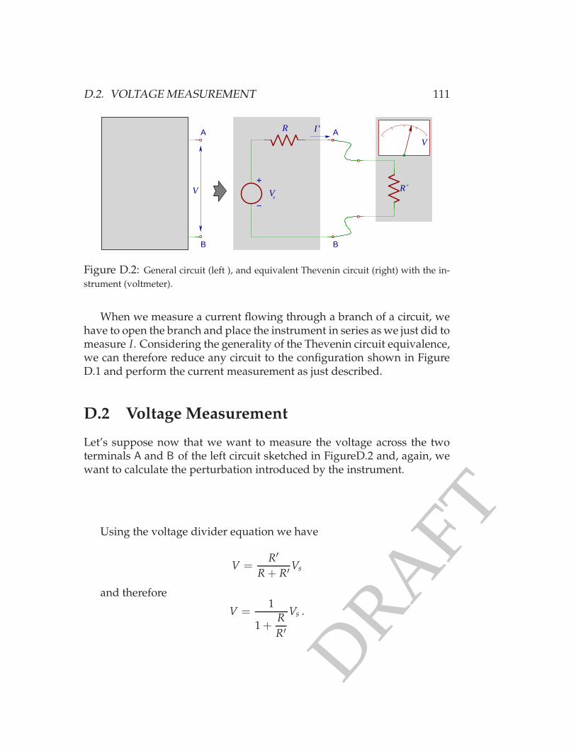
DRAFT

D.2. VOLTAGE MEASUREMENT 111

R´

I’

Vs

RA

B

V

VA

+

−

B

Figure D.2: General circuit (left ), and equivalent Thevenin circuit (right) with the in-

strument (voltmeter).

When we measure a current flowing through a branch of a circuit, wehave to open the branch and place the instrument in series as we just did tomeasure I. Considering the generality of the Thevenin circuit equivalence,we can therefore reduce any circuit to the configuration shown in FigureD.1 and perform the current measurement as just described.

D.2 Voltage Measurement

Let’s suppose now that we want to measure the voltage across the twoterminals A and B of the left circuit sketched in FigureD.2 and, again, wewant to calculate the perturbation introduced by the instrument.

Using the voltage divider equation we have

V =R′

R + R′Vs

and therefore

V =1

1 +R

R′

Vs .

DRAFT


We can conclude that the smaller the ratio R/R′ the more accurate themeasurement will be. A good voltmeter should have an input impedanceas large as possible.

Computing the relative uncertainty

∆V = Vs − V =R

R + R′Vs

∆V

Vs=

R

R + R′ =R

R′1

1 +R

R′

≃ R

R′

(

1 − R

R′

)

≃ R

R′

In words, the relative voltage perturbation to the circuit goes with the ratio of theresistance seen from the terminals A and B and of the instrument resistance.

The same consideration made for current measurements holds for volt-age measurements. We can always reduce any circuit to the configura-tion shown in FigureD.2 and perform the voltage measurement as just de-scribed.

D.3 AC Circuit Measurement Perturbation

It is straightforward to extend the previous results to the more general caseof circuits in the AC regime. In fact, it suffices to replace resistances withthe magnitude of a generic impedance.

For current measurements, we will have

|z||Z| ≪ 1 ⇒ |∆I|

|I| =|z|

|Z + z| ≃|z||Z| .

For voltage measurements, we will have

|Z||Z′| ≪ 1 ⇒ |∆V|

|V| =|Z|

|Z′ + Z| ≃|Z||Z′| .

D.3.1 Example: Oscilloscope

For the oscilloscope, we will have

Z′ = Rs +1

jωCs

DRAFT

D.3. AC CIRCUIT MEASUREMENT PERTURBATION 113

Supposing that

Z = R +1

jωC,

we will have

|∆V||V| ≃

∣

∣

∣

∣

∣

∣

∣

∣

R +1

jωC

Rs +1

jωCs

∣

∣

∣

∣

∣

∣

∣

∣

and therefore if

R ≪ Rs

C ≫ Cs

the oscilloscope voltage measurement will have a small systematic error.

DRAFT


DRAFT

Appendix E

Data Acquisition System“Experimenter”

The “Experimenter” device is a very simple data acquisition system (DAQ)which allows to acquire several channels with a low data rate. This are itsmain characteristics:

• maximum sampling frequency νs = 100samples/s

• Timer resolution ∆T = 2ms

• Input channels Characteristics

– Number : 4

– Number of bits: n = 10

– range : unipolar from 0V to 5.115V ⇒ ∆Vi = 5.115V

– resolution δVi = ∆Vi/2n = 5mV

• Output Channels Characteristics

– Number: 2

– Number of bits: n = 8

– type : unipolar

– range from 0 to 5V, ⇒ ∆Vo = 5V

– resolution: δVo = ∆Vo/2n ≃ 20mV (not linear)

– maximum current output: 1mA

115

DRAFT

116 APPENDIX E. DATA ACQUISITION SYSTEM “EXPERIMENTER”

0 50 100 150 200 250

0.5

1

1.5

2

2.5

3

3.5

4

4.5

DAC Input value (#)

DA

C O

utpu

t (V

)

Figure E.1: Output channel characteristics

E.1 Output Channel Characteristics

The output channel control is implemented using the so called pulse withmodulation (PWM) technique . Essentially, a PWM voltage source worksby changing the time that the pulse is on (the duty cycle), and sending thepulse to a low pass filter.

The non linearity of the output channel is clearly shown in the plotshown in figure E.1. The reason of such non-linearity comes from the waythat PWM is implemented.

DRAFT

E.2. EXPERTERM PROGRAM 117

E.2 ExperTerm Program

The “ExperTerm” is a terminal interface to communicate via RS232 port tothe DAQ. This is the list of the available commands:

• a ch0 [ch1] ... print ADC sampled value of channel ch0 ch1 ... Exam-ple: a 1

• A ch0 [ch1] ... continuously print ADC sampled values of channelch0 ch1 ... until a ctrl c is pressed. Example: A 1 0 3

• e ch val set voltage source ”ch” to ”val”. Example: e 0 124

• h print this help screen q quit program

E.3 ExperDAQ Program

The “ExperDAQ” is a command line program for continuous data acquisi-tion with the Experimenter. It allows to specify the acquisition parameters(input channels, number of samples, sampling frequency ) to change in-ternal relay status, and to set one voltage source. The following text is theprogram usage help:

usage: ExperDAQ [-v] [-p Port,BaudRate,Parity,Bits,StopBit] [-o Chan-nel,A,B,N] [-r] ChannelList Samples SamplingRate Averages FileName

Parameters between square brackets are optional.

• -v verbose mode.

• -p serial port configuration example: -p 1,9600,0,8,1

• -o Channel,A,B,N source output settings. Trailing spaces are not al-lowed

– Channel: 0 or 1

– A: initial value from 0 to 255

– B: final value from 0 to 255

– N: number of step to go from A to B. The step is done every1/SampleFrequency

DRAFT

118 APPENDIX E. DATA ACQUISITION SYSTEM “EXPERIMENTER”

• -r change relay status before data acquisition and restore previousstatus after the acquisition

• ChannelList: list of channels to acquire from 0 to 7. Values are sepa-rated with a comma. Trailing spaces are not allowed. Example: 3,0,1

• Samples number: samples to acquire

• SamplingRate: samples per seconds to acquire from 1 to 20

• Averages: number of averages. 0 for no averages. The data used tocompute the average are collected at the SamplingRate

• FileName: filename containing the acquired data. First column isthe time. The other columns are the channels values specified in theChannelList

Example:

ExperDAQ -r -o0,0,255,20 0,1,2 20 10 0 data.txt

The previous example does the following: change relay status duringthe acquisition, sweep the voltage source 0 from 0 to 255, acquires 20 sam-ples of ADC channels 0,1,2 with a sampling rate of 10sample/s, does notperform averages, and finally saves the data into the file data.txt.

freshman physics laboratory physics 3 course experiments - ligo

Documents