frequency scan–based mitigation approach of …
TRANSCRIPT

Frequency Scan–Based Mitigation Approach of SubsynchronousControl Interaction in Type-3 Wind Turbines
Faris M. Alatar
Thesis submitted to the Faculty of the
Virginia Polytechnic Institute and State University
in partial fulfillment of the requirements for the degree of
Master of Science
in
Electrical Engineering
Ali Mehrizi-Sani, Chair
Chen-Ching Liu
Vassilis Kekatos
July 26, 2021
Blacksburg, Virginia
Keywords: Frequency Scan, Resonance, Subsynchronous Control Interaction, Type-3 Wind
Turbines, Series Compensation, Wind Farm
Copyright 2021, Faris M. Alatar

Frequency Scan–Based Mitigation Approach of SubsynchronousControl Interaction in Type-3 Wind Turbines
Faris M. Alatar
ABSTRACT
Subsynchronous oscillations (SSO) were an issue that occurred in the past with conven-
tional generators and were studied extensively throughout the years. However, with the rise
of inverter-based resources, a new form of SSO emerged under the name subsynchronous
control interaction (SSCI). More specifically, a resonance case occurs between Type-3 wind
turbines and series compensation that can damage equipment within the wind farm and
disrupt power generation. This work explores the types of SSCI and the various analy-
sis methods as well as mitigation of SSCI. The work expands on the concept of frequency
scan to be able to use it in an on-line setting with its output data used to mitigate SSCI
through the modification of wind turbine parameters. Multiple frequency scans are con-
ducted using PSCAD/EMTDC software to build a lookup table and harmonic injection is
used in a parallel configuration to obtain the impedance of the system. Once the impedance
of the system is obtained then the value of the parameters is adjusted using the look-up
table. Harmonic injection is optimized through phase shifts to ensure minimal disruption
of the steady-state operating point and is conducted using Python programming language
with PSCAD Automation Library. Simulation results demonstrate the effectiveness of this
approach by ensuring oscillations do not grow exponentially in comparison to the regular
operation of the wind farm.

Frequency Scan–Based Mitigation Approach of SubsynchronousControl Interaction in Type-3 Wind Turbines
Faris M. Alatar
GENERAL AUDIENCE ABSTRACT
Due to climate change concern and the depletion of fossil fuel resources, electrical power
generation is shifting towards renewables such as solar and wind energy. Wind energy can
be obtained using wind turbines that transform wind energy into electrical energy, these
wind turbines come in four different types. Type-3 wind turbines are the most commonly
used in the industry which use a special configuration of the classical induction generator.
These wind turbines are typically installed in a distant location which makes it more difficult
to transfer energy from its location to populated areas, hence, series capacitors can be used
to increase the amount of transferred energy. However, these series capacitors can create a
phenomenon called subsynchronous control interaction (SSCI) with Type-3 wind turbines.
In this phenomenon, energy is exchanged back and forth between the series capacitors and
the wind turbines causing the current to grow exponentially which leads to interruptions
in service and damage to major equipments within the wind turbine. This work explores
SSCI, the tools to study it, and the currently available mitigation methods. It also presents
a method to identify the cases where SSCI can happen and mitigates it using adjustable
parameters.

Dedication
To my dear wife, Raja’.
iv

Acknowledgments
I would like to first thank my supervisor, Dr. Ali Mehrizi-Sani, for the enormous amount of
support that he has provided throughout this period. Even though we never had the chance
to meet personally, this was never an obstacle to his continuous support. Thanks go out for
his support whenever I felt desperate, his guidance whenever I was lost, and his continuous
and meticulous attention to detail.
A special thanks goes to Dr. Chen-Ching Liu and Dr. Vassilis Kekatos for the courses they
taught me. I will forever be grateful for the knowledge I gained from those courses. I am
also grateful to Dr. Virgilio Centeno, working as a GTA with Dr. Centeno for two semesters
was an amazing experience. I am thankful for him offering me the chance to teach.
I am grateful for having the opportunity to intern in Hitachi ABB Power Grids for a year.
A special thanks goes to my former boss, John Daniel, and colleagues, Jason, Eden, and
Adam, I learned so much from each one. Sidhaarth and Rahul for the gatherings and walks.
Ardavan and Yousef for the occasional hangouts. Ethan for the insight into college life. My
Jordanian friends for the trips and hangouts. I am also proud to be a Fulbrighter, thank
you Fulbright for the scholarship.
Finally, no words can describe my gratitude to my wife and family. Raja’, thank you for
everything, literally everything. Mom and Dad, thank you for providing me with the oppor-
tunities that led me here. Zain, thank you for your texts. Laith, thank you for your calls.
And to my friends Tillawi, Ala’a, Tafeeli, Amer, Jaber, Bashar, and Ibrahim, thank you for
sticking around.
A thesis during a pandemic, it wouldn’t have been possible if it weren’t for all of you.
Thanks everyone.
v

Contents
List of Figures ix
List of Tables xvi
1 Introduction 1
1.1 Background . . . . . . . . . . . . . . . . . . . . . . . . . . . . . . . . . . . . 1
1.2 Wind Energy . . . . . . . . . . . . . . . . . . . . . . . . . . . . . . . . . . . 2
1.3 Integration of Wind Energy . . . . . . . . . . . . . . . . . . . . . . . . . . . 4
1.4 Subsynchronous Oscillations (SSO) . . . . . . . . . . . . . . . . . . . . . . . 6
1.4.1 Subsynchronous Resonance (SSR) . . . . . . . . . . . . . . . . . . . . 7
1.4.2 Subsynchronous Torsional Interaction (SSTI) . . . . . . . . . . . . . 10
1.4.3 Subsynchronous Control Interaction (SSCI) . . . . . . . . . . . . . . 10
1.5 Thesis Outline . . . . . . . . . . . . . . . . . . . . . . . . . . . . . . . . . . 10
2 Subsynchronous Control Interaction (SSCI) 12
2.1 History of SSCI . . . . . . . . . . . . . . . . . . . . . . . . . . . . . . . . . . 12
2.2 Types of SSCI . . . . . . . . . . . . . . . . . . . . . . . . . . . . . . . . . . . 15
2.2.1 Series Capacitance . . . . . . . . . . . . . . . . . . . . . . . . . . . . 15
2.2.2 Weak Grid . . . . . . . . . . . . . . . . . . . . . . . . . . . . . . . . 15
vi

2.3 SSCI Features . . . . . . . . . . . . . . . . . . . . . . . . . . . . . . . . . . . 16
2.4 SSCI Analysis Methods . . . . . . . . . . . . . . . . . . . . . . . . . . . . . 18
2.4.1 Eigenvalue Analysis . . . . . . . . . . . . . . . . . . . . . . . . . . . 18
2.4.2 EMT Simulation Programs . . . . . . . . . . . . . . . . . . . . . . . 19
2.4.3 Impedance Modeling . . . . . . . . . . . . . . . . . . . . . . . . . . . 20
2.4.4 Frequency Scan . . . . . . . . . . . . . . . . . . . . . . . . . . . . . . 22
2.5 Mitigation of SSCI . . . . . . . . . . . . . . . . . . . . . . . . . . . . . . . . 23
2.5.1 System Planning Stage . . . . . . . . . . . . . . . . . . . . . . . . . . 24
2.5.2 Operation Stage . . . . . . . . . . . . . . . . . . . . . . . . . . . . . 24
2.5.3 Active Damping Control . . . . . . . . . . . . . . . . . . . . . . . . . 25
2.6 SSCI Protection . . . . . . . . . . . . . . . . . . . . . . . . . . . . . . . . . . 26
3 Frequency Scan for SSCI 27
3.1 Concept of Frequency Scans . . . . . . . . . . . . . . . . . . . . . . . . . . . 27
3.2 Studied System . . . . . . . . . . . . . . . . . . . . . . . . . . . . . . . . . . 29
3.3 Single Frequency Injection . . . . . . . . . . . . . . . . . . . . . . . . . . . . 30
3.4 Effect of Parameter Change on Impedance . . . . . . . . . . . . . . . . . . . 35
3.5 Effect of Online Turbines on Impedance . . . . . . . . . . . . . . . . . . . . 45
3.6 Effect of Power Order on Impedance . . . . . . . . . . . . . . . . . . . . . . 47
3.7 Multifrequency Injection . . . . . . . . . . . . . . . . . . . . . . . . . . . . . 48
vii

3.8 Verification of Multifrequency Injection Setup . . . . . . . . . . . . . . . . . 52
4 Frequency Scan Based Mitigation Approach of SSCI 56
4.1 Parallel Multifrequency Injection Scan . . . . . . . . . . . . . . . . . . . . . 56
4.2 Mitigation of SSCI Approach . . . . . . . . . . . . . . . . . . . . . . . . . . 60
4.3 Simulated Example of Mitigation Approach . . . . . . . . . . . . . . . . . . 62
4.3.1 Output Power Exceeds 1.050 pu . . . . . . . . . . . . . . . . . . . . . 62
4.3.2 Output Power Exceeds 1.025 pu . . . . . . . . . . . . . . . . . . . . . 63
4.3.3 Access to External Signal . . . . . . . . . . . . . . . . . . . . . . . . 64
4.3.4 Discussion . . . . . . . . . . . . . . . . . . . . . . . . . . . . . . . . . 65
5 Contributions and Future Work 67
Bibliography 68
Appendices 79
Appendix A System Scan Results 80
A.1 Variation of q-axis Proportional Gain . . . . . . . . . . . . . . . . . . . . . . 80
A.2 Variation of d-axis Proportional Gain . . . . . . . . . . . . . . . . . . . . . . 91
A.3 Variation of dq-axis Proportional Gain . . . . . . . . . . . . . . . . . . . . . 101
A.4 Variation of Online Turbines . . . . . . . . . . . . . . . . . . . . . . . . . . . 112
A.5 Variation of Power Order . . . . . . . . . . . . . . . . . . . . . . . . . . . . . 115
viii

List of Figures
1.1 Total installed renewable energy from 2011–2020. . . . . . . . . . . . . . . . 2
1.2 Wind turbine types. . . . . . . . . . . . . . . . . . . . . . . . . . . . . . . . 5
1.3 Classification of SSO. . . . . . . . . . . . . . . . . . . . . . . . . . . . . . . . 7
1.4 Equivalent circuit of DFIG. . . . . . . . . . . . . . . . . . . . . . . . . . . . 9
2.1 Current waveforms recorded in the Minnesota incident - Figure from Refer-
ence [25]. . . . . . . . . . . . . . . . . . . . . . . . . . . . . . . . . . . . . . 13
2.2 Weak grid SSCI demonstration. . . . . . . . . . . . . . . . . . . . . . . . . . 16
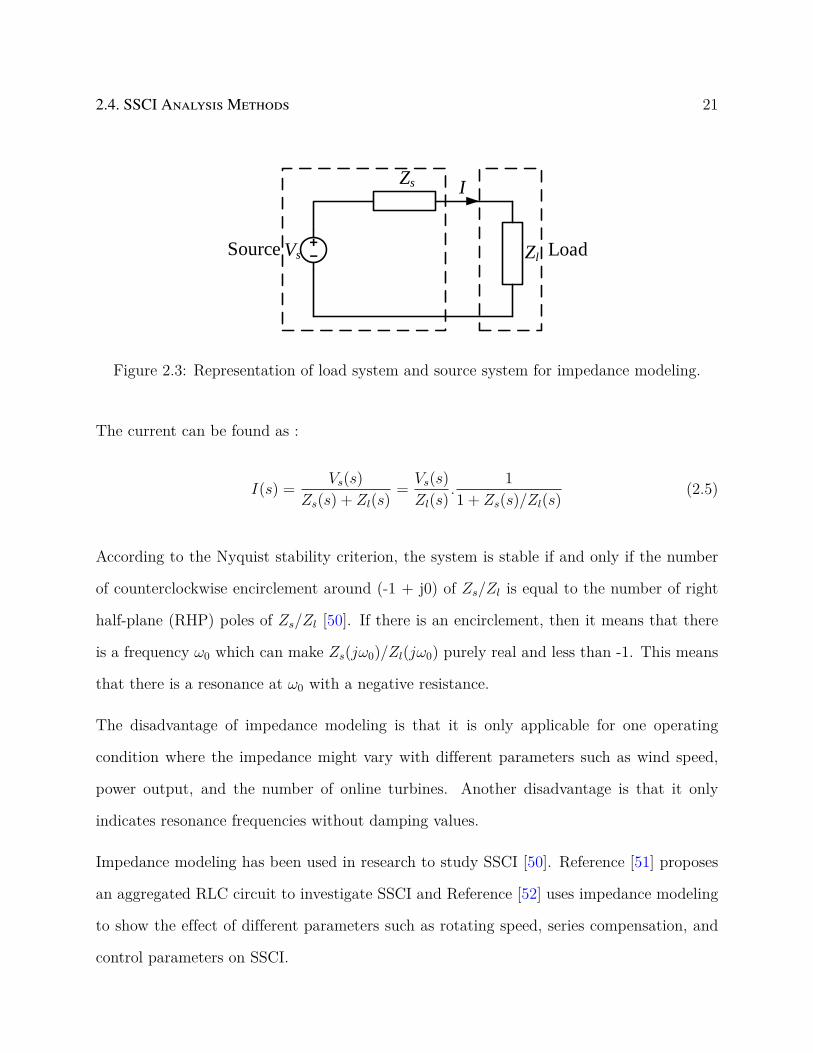
2.3 Representation of load system and source system for impedance modeling. . 21
3.1 Illustration of frequency scan system split. . . . . . . . . . . . . . . . . . . . 28
3.2 Modified IEEE second benchmark model. . . . . . . . . . . . . . . . . . . . 29
3.3 Frequency scan setup for WF side - single frequency injection. . . . . . . . . 31
3.4 Frequency scan setup for grid side - single frequency injection. . . . . . . . . 31
3.5 Frequency scan of WF side at 100% power order and 100% of online turbines. 32
3.6 Frequency scan of grid side before and after outage of line 2. . . . . . . . . . 33
3.7 System scan results before and after outage of line 2. . . . . . . . . . . . . . 34
3.8 DFIG block diagram, two back-to-back converters connect the rotor to the
grid, and the stator is directly connected to the grid. . . . . . . . . . . . . . 35
ix

3.9 RSC control loops: stator real power (top loop), and stator reactive power
(bottom loop). . . . . . . . . . . . . . . . . . . . . . . . . . . . . . . . . . . 36
3.10 GSC control loops: DC bus voltage (top loop), and grid-side reactive power
(bottom loop). . . . . . . . . . . . . . . . . . . . . . . . . . . . . . . . . . . 36
3.11 Frequency scan results for q-axis proportional gain variations (KpQ value in
legend). . . . . . . . . . . . . . . . . . . . . . . . . . . . . . . . . . . . . . . 37
3.12 Frequency scan results for d-axis proportional gain variations (Kpd value in
legend). . . . . . . . . . . . . . . . . . . . . . . . . . . . . . . . . . . . . . . 39
3.13 Frequency scan results for dq-axis proportional gains variations (Kpdq value
in legend). . . . . . . . . . . . . . . . . . . . . . . . . . . . . . . . . . . . . . 41
3.14 Γ-model induction generator model. . . . . . . . . . . . . . . . . . . . . . . . 41
3.15 System scan comparison between 2 Kpdq values. . . . . . . . . . . . . . . . . 44
3.16 Frequency scan results for various online turbines. . . . . . . . . . . . . . . . 45
3.17 Frequency scan results for various power orders. . . . . . . . . . . . . . . . . 46
3.18 Typical IGBT characteristic curve - Figure from Reference [80]. . . . . . . . 48
3.19 Multifrequency injection signal from 1 Hz to 60 Hz with δ = [0]n×1. . . . . . 53
3.20 Multifrequency injection signal from 1 Hz to 60 Hz with quadratic phase shift. 53
3.21 Multifrequency injection signal from 1 Hz to 60 Hz with Schroeder equation. 54
3.22 Multifrequency injection signal from 1 Hz to 60 Hz with optimized phases. . 54
3.23 Comparison between single frequency and multifrequency injections. . . . . . 55
4.1 Parallel scan setup in PSCAD/EMTDC. . . . . . . . . . . . . . . . . . . . . 56
x

4.2 Components of parallel scan box. . . . . . . . . . . . . . . . . . . . . . . . . 57
4.3 System impedance using parallel scan. . . . . . . . . . . . . . . . . . . . . . 58
4.4 Parallel scan impact on steady-state operation. . . . . . . . . . . . . . . . . 59
4.5 Flowchart of SSCI mitigation approach. . . . . . . . . . . . . . . . . . . . . 61
4.6 RMS voltage, real power, and reactive power waveforms for when output
power exceeds 1.050 pu. (black-dashed line is when line #2 trips, yellow-
dashed line is when SSCI is detected, and yellow straight line is when a stable
operating point is found). . . . . . . . . . . . . . . . . . . . . . . . . . . . . 63
4.7 RMS voltage, real power, and reactive power waveforms when output power
exceeds 1.025 pu. (black-dashed line is when line #2 trips, yellow-dashed line
is when SSCI is detected, and yellow straight line is when a stable operating
point is found). . . . . . . . . . . . . . . . . . . . . . . . . . . . . . . . . . . 64
4.8 RMS voltage, real power, and reactive power waveforms with access to ex-
ternal signal. (black-dashed line is when line #2 trips, yellow-dashed line is
when SSCI is detected, and yellow straight line is when a stable operating
point is found). . . . . . . . . . . . . . . . . . . . . . . . . . . . . . . . . . . 65
4.9 Comparison between no mitigation operation and the three mitigation ap-
proaches. . . . . . . . . . . . . . . . . . . . . . . . . . . . . . . . . . . . . . 66
A.1 System scan for Kpd = 2.00 and Kpq = 0.50. . . . . . . . . . . . . . . . . . . 81
A.2 System scan for Kpd = 2.00 and Kpq = 1.00. . . . . . . . . . . . . . . . . . . 81
A.3 System scan for Kpd = 2.00 and Kpq = 1.50. . . . . . . . . . . . . . . . . . . 82
A.4 System scan for Kpd = 2.00 and Kpq = 2.00. . . . . . . . . . . . . . . . . . . 82
xi

A.5 System scan for Kpd = 2.00 and Kpq = 2.50. . . . . . . . . . . . . . . . . . . 83
A.6 System scan for Kpd = 2.00 and Kpq = 3.00. . . . . . . . . . . . . . . . . . . 83
A.7 System scan for Kpd = 2.00 and Kpq = 3.50. . . . . . . . . . . . . . . . . . . 84
A.8 System scan for Kpd = 2.00 and Kpq = 4.00. . . . . . . . . . . . . . . . . . . 84
A.9 System scan for Kpd = 2.00 and Kpq = 4.50. . . . . . . . . . . . . . . . . . . 85
A.10 System scan for Kpd = 2.00 and Kpq = 5.00. . . . . . . . . . . . . . . . . . . 85
A.11 System scan for Kpd = 2.00 and Kpq = 5.50. . . . . . . . . . . . . . . . . . . 86
A.12 System scan for Kpd = 2.00 and Kpq = 6.00. . . . . . . . . . . . . . . . . . . 86
A.13 System scan for Kpd = 2.00 and Kpq = 6.50. . . . . . . . . . . . . . . . . . . 87
A.14 System scan for Kpd = 2.00 and Kpq = 7.00. . . . . . . . . . . . . . . . . . . 87
A.15 System scan for Kpd = 2.00 and Kpq = 7.50. . . . . . . . . . . . . . . . . . . 88
A.16 System scan for Kpd = 2.00 and Kpq = 8.00. . . . . . . . . . . . . . . . . . . 88
A.17 System scan for Kpd = 2.00 and Kpq = 8.50. . . . . . . . . . . . . . . . . . . 89
A.18 System scan for Kpd = 2.00 and Kpq = 9.00. . . . . . . . . . . . . . . . . . . 89
A.19 System scan for Kpd = 2.00 and Kpq = 9.50. . . . . . . . . . . . . . . . . . . 90
A.20 System scan for Kpd = 2.00 and Kpq = 10.00. . . . . . . . . . . . . . . . . . . 90
A.21 System scan for Kpd = 0.50 and Kpq = 2.00. . . . . . . . . . . . . . . . . . . 91
A.22 System scan for Kpd = 1.00 and Kpq = 2.00. . . . . . . . . . . . . . . . . . . 92
A.23 System scan for Kpd = 1.50 and Kpq = 2.00. . . . . . . . . . . . . . . . . . . 92
A.24 System scan for Kpd = 2.50 and Kpq = 2.00. . . . . . . . . . . . . . . . . . . 93
xii

A.25 System scan for Kpd = 3.00 and Kpq = 2.00. . . . . . . . . . . . . . . . . . . 93
A.26 System scan for Kpd = 3.50 and Kpq = 2.00. . . . . . . . . . . . . . . . . . . 94
A.27 System scan for Kpd = 4.00 and Kpq = 2.00. . . . . . . . . . . . . . . . . . . 94
A.28 System scan for Kpd = 4.50 and Kpq = 2.00. . . . . . . . . . . . . . . . . . . 95
A.29 System scan for Kpd = 5.00 and Kpq = 2.00. . . . . . . . . . . . . . . . . . . 95
A.30 System scan for Kpd = 5.50 and Kpq = 2.00. . . . . . . . . . . . . . . . . . . 96
A.31 System scan for Kpd = 6.00 and Kpq = 2.00. . . . . . . . . . . . . . . . . . . 96
A.32 System scan for Kpd = 6.50 and Kpq = 2.00. . . . . . . . . . . . . . . . . . . 97
A.33 System scan for Kpd = 7.00 and Kpq = 2.00. . . . . . . . . . . . . . . . . . . 97
A.34 System scan for Kpd = 7.50 and Kpq = 2.00. . . . . . . . . . . . . . . . . . . 98
A.35 System scan for Kpd = 8.00 and Kpq = 2.00. . . . . . . . . . . . . . . . . . . 98
A.36 System scan for Kpd = 8.50 and Kpq = 2.00 . . . . . . . . . . . . . . . . . . 99
A.37 System scan for Kpd = 9.00 and Kpq = 2.00. . . . . . . . . . . . . . . . . . . 99
A.38 System scan for Kpd = 9.50 and Kpq = 2.00. . . . . . . . . . . . . . . . . . . 100
A.39 System scan for Kpd = 10.00 and Kpq = 2.00. . . . . . . . . . . . . . . . . . . 100
A.40 System scan for Kpd = 0.50 and Kpq = 0.50. . . . . . . . . . . . . . . . . . . 102
A.41 System scan for Kpd = 1.00 and Kpq = 1.00. . . . . . . . . . . . . . . . . . . 102
A.42 System scan for Kpd = 1.50 and Kpq = 1.50. . . . . . . . . . . . . . . . . . . 103
A.43 System scan for Kpd = 2.50 and Kpq = 2.50. . . . . . . . . . . . . . . . . . . 103
A.44 System scan for Kpd = 3.00 and Kpq = 3.00. . . . . . . . . . . . . . . . . . . 104
xiii

A.45 System scan for Kpd = 3.50 and Kpq = 3.50. . . . . . . . . . . . . . . . . . . 104
A.46 System scan for Kpd = 4.00 and Kpq = 4.00. . . . . . . . . . . . . . . . . . . 105
A.47 System scan for Kpd = 4.50 and Kpq = 4.50. . . . . . . . . . . . . . . . . . . 105
A.48 System scan for Kpd = 5.00 and Kpq = 5.00. . . . . . . . . . . . . . . . . . . 106
A.49 System scan for Kpd = 5.50 and Kpq = 5.50. . . . . . . . . . . . . . . . . . . 106
A.50 System scan for Kpd = 6.00 and Kpq = 6.00. . . . . . . . . . . . . . . . . . . 107
A.51 System scan for Kpd = 6.50 and Kpq = 6.50. . . . . . . . . . . . . . . . . . . 107
A.52 System scan for Kpd = 7.00 and Kpq = 7.00. . . . . . . . . . . . . . . . . . . 108
A.53 System scan for Kpd = 7.50 and Kpq = 7.50. . . . . . . . . . . . . . . . . . . 108
A.54 System scan for Kpd = 8.00 and Kpq = 8.00. . . . . . . . . . . . . . . . . . . 109
A.55 System scan for Kpd = 8.50 and Kpq = 8.50. . . . . . . . . . . . . . . . . . . 109
A.56 System scan for Kpd = 9.00 and Kpq = 9.00. . . . . . . . . . . . . . . . . . . 110
A.57 System scan for Kpd = 9.50 and Kpq = 9.50. . . . . . . . . . . . . . . . . . . 110
A.58 System scan for Kpd = 10.00 and Kpq = 10.00. . . . . . . . . . . . . . . . . . 111
A.59 System scan for 100% online turbines. . . . . . . . . . . . . . . . . . . . . . 112
A.60 System scan for 50% online turbines. . . . . . . . . . . . . . . . . . . . . . . 113
A.61 System scan for 25% online turbines. . . . . . . . . . . . . . . . . . . . . . . 113
A.62 System scan for 10% online turbines. . . . . . . . . . . . . . . . . . . . . . . 114
A.63 System scan for 100% power order. . . . . . . . . . . . . . . . . . . . . . . . 115
A.64 System scan for 50% power order. . . . . . . . . . . . . . . . . . . . . . . . . 116
xiv

A.65 System scan for 25% power order. . . . . . . . . . . . . . . . . . . . . . . . . 116
A.66 System scan for 10% power order. . . . . . . . . . . . . . . . . . . . . . . . . 117
xv

List of Tables
1.1 Frequencies of currents in stator and rotor of the DFIG . . . . . . . . . . . . 9
2.1 List of previous SSCI incidents . . . . . . . . . . . . . . . . . . . . . . . . . 14
2.2 SSCI analysis methods summary . . . . . . . . . . . . . . . . . . . . . . . . 23
3.1 Line parameters for modified IEEE second benchmark model . . . . . . . . . 29
3.2 Crossover frequency and resistance values for q-axis proportional gain variations 38
3.3 Crossover frequency and resistance values for d-axis proportional gain variations 40
3.4 Crossover frequency and resistance values for dq-axis proportional gains vari-
ations . . . . . . . . . . . . . . . . . . . . . . . . . . . . . . . . . . . . . . . 42
3.5 Crossover frequency and resistance values for various online turbines . . . . . 46
3.6 Crossover frequency and resistance values for various power orders . . . . . . 47
3.7 Peak values of multifrequency injection . . . . . . . . . . . . . . . . . . . . . 51
3.8 Crossover frequency and resistance values for single frequency and multifre-
quency injections . . . . . . . . . . . . . . . . . . . . . . . . . . . . . . . . . 52
4.1 Comparison between the three mitigation approaches . . . . . . . . . . . . . 66
xvi

List of Abbreviations
DFIG Doubly-Fed Induction Generator
DFR Digital Fault Recorder
FACTS Flexible AC Transmission System
GSC Grid Side Converter
HVDC High Voltage DC
IBR Inverter-Based Resource
IGE Induction Generator Effect
PSS Power System Stabilizer
RSC Rotor Side Converter
SSCI Subsynchronous Control Interaction
SSO Subsynchronous Oscillation
SSR Subsynchronous Resonance
SSTI Subsynchronous Torsional Interaction
SVC Static VAR Compensator
TA Torque Amplification
TI Torsional Interaction
xvii

VSC Voltage-Sourced Converter
WF Wind Farm
WPP Wind Power Plant
WT Wind Turbine
xviii

Chapter 1
Introduction
1.1 Background
Throughout history, power systems have been experiencing increased stress due to the in-
creased dependency on electricity in multiple sectors, global economic growth and increased
populations. As more and more sectors rely on electricity for their operation, such as trans-
portation, space heating, and some industrial processes, ensuring a continuous supply of
electrical power becomes a more challenging task and one of critical importance [1]. Several
events in history, such as the Northeast blackout of 2003, and the 2019 GB blackout, have
showed the enormous financial losses, and the disruption of services to customers that can
occur due to faults and errors in electrical power systems [2].
Power systems have long been operated in a traditional and conventional way, where the
dominating power generation was done by non-renewable energy sources such as coal, natural
gas, and oil. Driven by climate concerns, decreasing costs, and the depletion of fossil fuels,
power generation is shifting towards using renewable energy sources in an accelerating pace.
The usage of renewable energy has been increasing throughout the last decade as shown in
Figure 1.1 where the net addition of renewable energy in 2020 exceeded that in 2019 by 50%
[3].
As more and more sectors increasingly rely on electricity, this figure is only expected to
1

2 CHAPTER 1. INTRODUCTION
increase. According to the International Energy Agency (IEA), an additional 22,101 TWh
is expected to be generated from renewable sources by 2040 while non-renewable energy
production is expected to drop by a value of 9,664 TWh in the same period [4].
Figure 1.1: Total installed renewable energy from 2011–2020.
1.2 Wind Energy
One of the most prominent sources of renewable energy is wind energy. This is because of the
massive production potential that wind can offer. Wind energy has been used throughout
human civilization in mills, sailing, and pumping. Wind energy has proven to be one of the
most viable choices for clean energy production and has been utilized in power generation
through the use of wind turbine (WT), where the basic working principle is to convert wind
energy into mechanical energy and in turn into electrical energy that can be utilized.
WTs can assist in power generation without affecting the climate. This is due to not pro-
ducing greenhouse gas emissions, and using little land area in comparison to other renewable

1.2. WIND ENERGY 3
energy sources. In addition to this, the cost of WTs has been declining due to increasing
capacity factors where larger towers with bigger blades are being developed and installed [5].
WTs have developed throughout history, and the technology used in them has advanced.
They were first used to cover local energy demands but then started to get connected to the
electrical grid. WTs are mainly divided into fixed-speed turbines, and variable speed turbines
- where the variable speed operation is made possible due to the usage of power electronic
components. Variable speed operated WTs have several advantages over fixed-speed. Some
of which include a better utilization of wind energy, less mechanical stress, along with better
control capabilities.
WTs have drastically changed during the past 30 years and can now be categorized into four
main types according to the AC generator and converter types used in them, as shown in
Figure 1.2:
1. Type-1 WT - use squirrel cage induction generators (SCIG) operating at a fixed speed
that need complex considerations in the development of mechanical parts with limited
control capabilities. A capacitor bank is needed to compensate for the reactive power
demand from the SCIG [6].
2. Type-2 WT - use wound rotor induction generators (WRIG) with adjustable rotor
resistance control for better control capabilities. The main disadvantage of this type is
that the limited controllability comes at the expense of efficiency due to energy being
wasted in the rotor resistance along with the capacitor bank requirement for reactive
power compensation.
3. Type-3 WT - use doubly-fed induction generators (DFIG), this type can provide its
own reactive power. The power converters used in this type only need to handle 30%
of the rated turbine power.

4 CHAPTER 1. INTRODUCTION
4. Type-4 WT - use permanent magnet synchronous generators (PMSG) with full power
converters, this type can provide its own reactive power as well. An advantage of this
type is that the gearbox can be eliminated thus reducing the overall mechanical stress.
The disadvantage of this type is that the power converters need to be able to handle
the full rated turbine power.
The first two types of turbines were used in the first stages of wind turbine installations.
However, recently, most installed WTs are either Type-3 or Type-4 WTs [7]. According to
the Global Wind Energy Council (GWEC), the global wind energy market is expected to
grow on average by 4% each year in the next five years [8].
1.3 Integration of Wind Energy
WTs did not leave a serious impact on the power grid system at their early stages, where
wind fluctuations were directly transferred into the grid, and they lacked reactive and active
powers’ controllability. However, as more WTs got installed and wind penetration increased
in the grid, these previously neglected issues became more noticeable and needed to be
addressed. This has been made possible mostly due to the advancement in power electronics
that has allowed for WTs to become an active power generation unit instead of an unregulated
power source. Nevertheless, the integration of WTs into the electrical grid comes with issues
that can be mainly categorized into two main types; operational issues and dynamic issues
[9].
Operational issues are related to the fact that wind energy is not dispatchable, thus creating
the complexity of having to rely on an intermittent power source due to the nature of wind
energy. In [10], a two stage stochastic programming was proven to be effective to overcome
the uncertainty with real time decisions.

1.3. INTEGRATION OF WIND ENERGY 5
Gear
Box
Induction
Generator
PFC
Capacitors
Turbine
Transformers
Collector
Bus
Grid
Gear
Box
Induction
Generator
PFC
Capacitors
Turbine
Transformers
Collector
Bus
Grid
Gear
Box
DFIGTurbine
Transformers
Collector
Bus
Grid
PMSGTurbine
Transformers
Collector
Bus
Grid
(a) Type-1 Wind Turbine
(b) Type-2 Wind Turbine
(c) Type-3 Wind Turbine
(d) Type-4 Wind Turbine
Variable
Resistor
RSC GSC
PWM Converter
Figure 1.2: Wind turbine types.

6 CHAPTER 1. INTRODUCTION
Dynamic issues, however, are short in the nature of their time-scale. These issues are mostly
related to fault handling, inter-area oscillations, resonances (both electrical and electrome-
chanical) and interactions.
Typically, wind farms are installed in locations that are far away from load centers. There-
fore, the power generated must be transferred to load centers through either new or existing
transmission lines [11]. New transmission lines require a significant investment, therefore,
a better utilization of already existing transmission lines is almost always desired. Series
compensation allows for this enhanced utilization by reducing the total inductive reactance
of the line, and it also improves the stability and contrallibility in the grid, resulting in
increasing the total available transfer capability of the existing line [12]. That said, series
compensation does give rise to one type of dynamic issues called subsynchronous oscillations
(SSO).
1.4 Subsynchronous Oscillations (SSO)
SSO are oscillations that have a frequency below the fundamental frequency [13], and can
damage components in the power system, as well as disrupting the operation of the power
system. SSO can be classified into three main types, as depicted in Figure 1.3:
1. Subsynchronous Resonance (SSR)
(a) Induction Generator Effect (IGE)
(b) Torsional Interaction (TI)
2. Subsynchronous Torsional Interactional (SSTI)
3. Subsynchronous Control Interaction (SSCI)

1.4. SUBSYNCHRONOUS OSCILLATIONS (SSO) 7
Sub-Synchronous Oscillations (SSO)
Sub-Synchronous Resonance (SSR)
Induction Generator Effect (IGE)
Torsional Interaction (TI)
Sub-Synchronous Torsional Interaction
(SSTI)
Sub-Synchronous Control Interaction
(SSCI)
Figure 1.3: Classification of SSO.
1.4.1 Subsynchronous Resonance (SSR)
SSR is ”an electric power system condition where the electric network exchanges energy with
a turbine generator at one or more of the natural frequencies of the combined system below
its synchronous frequency” as defined by IEEE [14]. This includes both natural modes of
oscillation due to inherent system characteristics, and forced modes of oscillation that are
driven by a particular device or control system.
The first paper to ever discuss the possibility of an interaction between turbine generators
and series compensation was published in 1937 [15]. However, it only got the full attention
of researchers when the first case of SSR occurred at the Mohave coal-fired power plant back
in 1970 and 1971 which resulted in fractures of the shafts of the turbine generator [16]. It
8 CHAPTER 1. INTRODUCTION
was initially reported to be a mechanical failure but it was later identified correctly after the
second incident to be a case of SSR and was addressed in a paper in 1973 [17].
Induction Generator Effect (IGE)
IGE is a purely electrical phenomenon that involves the interaction between the series-
compensated line and the negative damping in DFIG at the resonance frequency.
The resonance frequency of a series compensated line is
fssr = fs
√Xc
XL
= fs√k (1.1)
where
fs is the synchronous frequency of the system
Xc is the series capacitor reactance
XL is the transmission line inductive reactance
k is the percentage of series compensation for the transmission line.
At fssr, the slip will be:
sssr =fssr − frfssr
(1.2)
where
fr is the electrical frequency of the rotor.
At fssr, which is typically below fr, the slip will be negative. The steady-state equivalent
circuit of DFIG using a classical induction machine representation is shown in Figure 1.4.
Having a negative slip results in a negative Rr which can overcome the positive resistance in
the remainder of the system (transmission line and stator resistance), resulting in a negative

1.4. SUBSYNCHRONOUS OSCILLATIONS (SSO) 9
system damping at fssr [18].
Figure 1.4: Equivalent circuit of DFIG.
The frequencies of currents in the stator and rotor are listed in Table 1.1 [9].
Table 1.1: Frequencies of currents in stator and rotor of the DFIG
Stator Current Rotor Electrical Frequency Rotor Current
Is1 → fs fr Ir1 → fs − frIs2 → fssr fr Ir2 → fssr − fr
Torsional Interaction (TI)
TI is the interplay between the mechanical system and electrical system represented by
the turbine-generator and the series-compensated line, respectively [19]. In this case, the
generator rotor oscillations grow undamped when the induced subsynchronous frequency
matches one of the natural oscillatory modes of the turbine generator shaft [20]. TI is more
likely to take place in conventional plants with low inertia and is not a typical risk in WTs.

10 CHAPTER 1. INTRODUCTION
1.4.2 Subsynchronous Torsional Interaction (SSTI)
SSTI is another known problem where the mechanical mass of a synchronous generator
resonates with the negative damping of a nearby power electronic controller and can cause
damage to generators. It is a device-dependent interaction which requires the presence of
power electronic controllers such as those found in FACTS, SVC, PSS, and HVDC links that
typically respond quickly to power variations where these controllers can exhibit negative
damping at subsynchronous frequencies [21]. The first SSTI incident involved an HVDC line
in Square Butte that connects North Dakota and Minnesota [22].
1.4.3 Subsynchronous Control Interaction (SSCI)
SSCI is a device-dependent type of SSO that is caused by an interaction between inverter-
based resources (IBR), and either series compensation or weak grid conditions. Typically,
any SSO that involves Type-3 and Type-4 WTs is categorized as a SSCI case. SSCI will be
further explained and discussed in Chapter 2.
1.5 Thesis Outline
The thesis is outlined as the following:
• Chapter 1 provides a background for renewable energy, wind energy, the integration
of WTs, and an introduction to SSR.
• Chapter 2 describes the SSCI phenomenon, study approaches, and mitigation methods.
• Chapter 3 describes the frequency scan study approach, and presents a different ap-
proach to frequency scans.
1.5. THESIS OUTLINE 11
• Chapter 4 presents a mitigation approach to prevent SSCI using on-line frequency
scan, and parameter modification of DFIG or wind farms.
• Chapter 5 is the conclusion and future work related to this thesis.

Chapter 2
Subsynchronous Control Interaction
(SSCI)
2.1 History of SSCI
The first incident of subsynchronous oscillations (SSO) related to wind turbines (WTs) oc-
curred back in 2007 in Minnesota [23] following an installation of 60% series compensation
on a 34 kV transmission line. Prior to installing the series compensation, SSO susceptibil-
ity studies were conducted as usual to assess the risk of SSO with the nearby conventional
generators. Transfer trip schemes were installed as a cautionary measure despite the studies
showing no significant risk of SSO. It was assumed at that time that Type-3 WT will be
immune to these oscillations due to their partial isolation with the usage of power electronics
[24].
However, three days after the installation of the series compensation, and after a normal
scheduled system outage for nearby breakers, the wind farm (WF) was left in a radial con-
nection with the series capacitor resulting in undamped current oscillations which damaged
components within some of the WTs.
Through the analysis following the event using the waveform traces collected by the digi-
12

2.1. HISTORY OF SSCI 13
tal fault recorders (DFR)1, it was identified that one frequency component (9.44 Hz) had
negative damping and four other frequency components (38.85 Hz, 59.86 Hz, 60.32 Hz, and
62.83 Hz) had damping of less than 1% [25]. The magnitude of the phase current peak
increased ten folds within 0.3 s as shown in Figure 2.1.
Figure 2.1: Current waveforms recorded in the Minnesota incident - Figure from Reference[25].
The frequencies of the oscillations did not coincide with any of the modal frequencies of
the nearby combustion turbine generators shafts nor with the Eigen frequencies of the WTs
structures.
The first subsynchronous control interaction (SSCI) incident to cause severe damage was
witnessed within the Electric Reliability Council of Texas (ERCOT) grid in 2009 [26] that1Even though the radial connection remained for almost five minutes, only the first second was captured
by the DFRs.

14 CHAPTER 2. SUBSYNCHRONOUS CONTROL INTERACTION (SSCI)
involved Type-3 WTs, and resulted in 20-30 Hz oscillations [27]. In 2011, 4 Hz oscillations
were observed in Type-4 WTs in Texas following a transmission outage [28]. Another incident
in Texas that also involved Type-3 WTs occurred in 2017 in three different events with the
same frequency range of oscillations between 20-30 Hz [29].
Throughout the years 2012 to 2016, multiple SSCI incidents were also witnessed in Xinjiang
as well as in northern regions of China that included both Type-3 and Type-4 WTs. After
this incident, multiple incidents occurred within the ERCOT grid and China grid [30]. These
incidents occurred frequently; for example, 58 SSCI events were detected within a one-year
span in Northern China. As well as that, some of these incidents involved a significantly
lower percentage of series compensation in comparison to the Minnesota and Texas incidents.
The last incident related to SSCI up to date occurred in 2019 in Great Britain (GB) when
an undamped electric resonance between an off-shore WF that consists of Type-4 WTs along
with weak grid conditions resulted in a voltage drop that led to the disconnection of Hornsea
offshore WF that ended up in an enormous blackout in Great Britain grid [31]. Table 2.1
summarizes the list of incidents related to SSCI.
Table 2.1: List of previous SSCI incidents
Year(s) Location WT Type Interaction With
2007 Minnesota Type-3 Series compensation2009 Texas Type-3 Series compensation2011 Texas Type-4 Weak grid
2012-2016 Northern China Type-3 Series compensation2014-2015 Xinjiang, China Type-4 Weak grid
2017 Texas Type-3 Series compensation2019 UK Type-4 Weak grid

2.2. TYPES OF SSCI 15
2.2 Types of SSCI
SSCI can be divided into two main types [32] depending on the WT type:
1. SSCI with series capacitance
2. SSCI with weak grid
2.2.1 Series Capacitance
This type of SSCI occurs in Type-3 WT where an interaction occurs between the voltage-
sourced converters (VSCs) in the WT and the series capacitor. The mechanism of this
SSCI is nearly identical to IGE, which was previously explained in 1.4.1, where the overall
resistance is negative at the resonance frequency resulting in undamped oscillations. A radial
connection between a series-compensated line and a WF significantly increases the risk of
SSCI due to the reduction in system inductive impedance thus effectively increasing the
system capacitive impedance.
2.2.2 Weak Grid
This type of SSCI occurs in Type-4 WT which mainly happens in VSCs that are connected
to weak grid conditions. An instability loop is introduced due to the coupling between the
POI voltage and the WT power output. A simple system, for illustration purposes, is shown
in Figure 2.2. The connected WT is modeled in dq-frame aligned with the POI voltage

16 CHAPTER 2. SUBSYNCHRONOUS CONTROL INTERACTION (SSCI)
(d-axis voltage aligned to the POI voltage). Therefore,
∆V = ∆vd
= −X∆iq −X√(
V∞Xid
)2
− 1
∆id(2.1)
The output power is defined as
P = V id ∴ ∆P = id∆V + V∆id (2.2)
Figure 2.2: Weak grid SSCI demonstration.
The instability is introduced as whenever the power order increases, id increases. However,
that also reduces the value of the POI voltage which effectively reduces the power output of
the WT [33].
2.3 SSCI Features
According to the definition in [19], SSCI can be listed under the category of Device Depen-
dent Subsynchronous Oscillations (DDSO) where SSCI has distinctive features which makes
it different than other SSO cases. The first difference is that subsynchronous resonance (SSR)
does not include power electronic converters unlike SSCI and subsynchronous torsional inter-
action (SSTI) where power electronic converters actively participate in the oscillations. The

2.3. SSCI FEATURES 17
involvement of power electronic converters makes it difficult to use approaches previously
used in SSR in SSCI cases.
In addition to this, SSR is usually associated with conventional steam turbine generators
(STGs) unlike SSCI which is associated with wind turbine generators (WTGs). The differ-
ences between WTGs and STGs are vast, such as power generation capacity (WTGs range
in a few megawatts unlike STGs which can exceed hundreds of megawatts), and the number
of generators in a WF is significantly larger than the number of generators in a conventional
power plant. This makes it very difficult to model the entire WF for SSCI analysis, and thus
these generators in a WF must be aggregated [34].
The third difference is that SSR and SSTI typically involve mechanical shaft dynamics
whereas SSCI is an electrical phenomenon that does not include any torsional oscillations
[35]. The last and fourth difference is that oscillations due to SSR and SSTI happen at a
fixed frequency unlike SSCI where they vary with different parameters such as wind speed,
number of WTs in service, grid stiffness, and control parameters of the WTs.

18 CHAPTER 2. SUBSYNCHRONOUS CONTROL INTERACTION (SSCI)
2.4 SSCI Analysis Methods
Four main methods and tools can be used to study and investigate the risk of SSCI in wind
farms. Each provide their own advantages and come with their own disadvantages.
2.4.1 Eigenvalue Analysis
Eigenvalue analysis is a powerful method to study SSCI where the complete system must be
linearized at a steady-state operating point in the form of:
x = Ax+Bu (2.3)
where the eigenvalues of the system can be obtained by solving:
det[λI −A] = 0 (2.4)
The obtained eigenvalues contains all frequencies of oscillations along with their respective
damping values. Eigenvalue analysis can also be used to study participation factors for each
component, as well as residue analysis for controller design. MATLAB is one of the most
commonly used softwares to conduct this analysis.
However, eigenvalue analysis requires high-order mathematical models which can make the
modeling process complex, and it also requires significant computational time and effort to
use taking into account the physical non-linearities, and the presence of switching devices
[36]. As well as this, manufacturers of WTs typically provide black-box models for their WTs
due to intellectual property rights which makes the usage of eigenvalue analysis impossible
to conduct without gaining access to the WT internal system [34].

2.4. SSCI ANALYSIS METHODS 19
Eigenvalue analysis is used extensively in research work in order to investigate SSCI. Refer-
ences [9] and [37] say that eigenvalue analysis is used to study SSCI in Type-3 WTs connected
to series compensation, and the participation factors of different parameters including the
percentage of series compensation and wind speed. It also did a feasibility test of using
eigenvalue analysis to identify and select proper mitigation signals for SSCI.
Grid connected Type-3 WTs were modeled extensively, and their behavior was studied in
Reference [38]. The first IEEE benchmark model for subsynchronous resonance studies was
modified in Reference [39] to connect 100 MW of Type-3 WTs to study SSCI using eigenvalue
analysis.
2.4.2 EMT Simulation Programs
Electromagnetic transient (EMT) programs use models which include sufficient detail in
order to simulate the dynamics of the system including power electronic converters, and
their control systems in the time domain unlike traditional transient stability programs
which are based in the frequency domain using phasors that will not be able to simulate
subsynchronous frequencies’ dynamics.
EMT programs require detailed models of the system components including the WT and its
control. These models are typically provided by the wind manufacturer in a black-box. One
of the advantages of EMT programs is that once the system has been modeled, then the
system can be used for small signal and large signal analysis. It can also serve as a validation
check for results obtained using other methods.
The disadvantage of EMT programs is that they are computationally expensive due to the
small time-steps required for switching devices. As well as this, they do not indicate the
potential risks that can arise in the future.

20 CHAPTER 2. SUBSYNCHRONOUS CONTROL INTERACTION (SSCI)
EMT programs can be software-based or hardware-based. PSCAD/EMTDC and MAT-
LAB/Simulink are the most commonly used software-based EMT programs where multiple
papers studied SSCI using them [36, 40, 41, 42, 43], while RTDS and OPAL-RT are the
most commonly used hardware-based EMT programs, and have been used in research as
well [44, 45, 46]. The configuration for hardware-based simulations is controller hardware in
the loop (CHIL) in order to simulate SSCI using physical WT controllers. The work in this
thesis will use PSCAD as the software-based EMT program in addition to frequency scans.
2.4.3 Impedance Modeling
Impedance modeling is a small signal modeling method which describes the system with
an input-output relationship (voltage and current) in the frequency domain. Once the
impedance model has been calculated, the Nyquist stability criterion can be used to de-
termine the stability of the system. It was first introduced back in 1976 [47] and has been
used extensively in black-box systems [48].
Depending on the components in the system, the impedance can be obtained either through
the analytical method, or through the measurement method. In the analytical method, the
components and the parameters of the components must be known, where the impedance is
calculated by applying the linearization theory where if there is a current disturbance at the
terminal then the resulting voltage is measured in order to obtain the impedance value [49].
This can either be done in the dq rotating domain or the abc stationary domain is applied
and the voltage response is measured to obtain the impedance value.
The WT system is divided into two segments; the source system and the load system where
each have their own impedance as shown in Figure 2.3.
2.4. SSCI ANALYSIS METHODS 21
Zs
ZlVs
I
Source Load
Figure 2.3: Representation of load system and source system for impedance modeling.
The current can be found as :
I(s) =Vs(s)
Zs(s) + Zl(s)=Vs(s)
Zl(s).
1
1 + Zs(s)/Zl(s)(2.5)
According to the Nyquist stability criterion, the system is stable if and only if the number
of counterclockwise encirclement around (-1 + j0) of Zs/Zl is equal to the number of right
half-plane (RHP) poles of Zs/Zl [50]. If there is an encirclement, then it means that there
is a frequency ω0 which can make Zs(jω0)/Zl(jω0) purely real and less than -1. This means
that there is a resonance at ω0 with a negative resistance.
The disadvantage of impedance modeling is that it is only applicable for one operating
condition where the impedance might vary with different parameters such as wind speed,
power output, and the number of online turbines. Another disadvantage is that it only
indicates resonance frequencies without damping values.
Impedance modeling has been used in research to study SSCI [50]. Reference [51] proposes
an aggregated RLC circuit to investigate SSCI and Reference [52] uses impedance modeling
to show the effect of different parameters such as rotating speed, series compensation, and
control parameters on SSCI.

22 CHAPTER 2. SUBSYNCHRONOUS CONTROL INTERACTION (SSCI)
2.4.4 Frequency Scan
Frequency scan is one of the most commonly used tools to investigate SSCI, more specifically
it is widely used in dealing with black-box models. Ideally, a frequency scan works by mea-
suring the impedance of the system from the stator windings. However, the more common
approach is to scan the entire WF and the system separately to obtain their impedances.
Once these impedances are found, then they are lumped into one impedance Zsys(f) where
it is then divided into resistance (real part) Rsys(f), and reactance Xsys(f) (imaginary part)
[53].
The resistance Rsys(f) and reactance Xsys(f) are then plotted against frequency f , and
resonance frequencies are identified in the reactance plot, if the resistance is negative then
the system is unstable, otherwise, the system is considered stable.
The advantage of this method is the ability for it to be used with black-box models, since
it mainly works on measuring the output related to a certain input without having to know
the exact configuration, parameters or topology of the WTs.
The disadvantage of frequency scans is that they are only applicable for one operating con-
dition where the impedance values vary with wind speed, series compensation, and different
parameters of WT controllers. Another disadvantage is that they can only be used to identify
the resonance frequencies without damping values.
Reference [51] proposed a method for identifying the damping values using frequency scans
using aggregated RLC circuit. Reference [54] used the frequency scan method but based it
on the slope of resistance and reactance curves instead of looking for resonance frequencies
and negative resistances.
The work in this thesis will also use frequency scans and will be further explained in Chapter

2.5. MITIGATION OF SSCI 23
Table 2.2: SSCI analysis methods summary
Method Advantages Disadvantages
Eigenvalue AnalysisIdentifies oscillatory frequencies withdamping values
Requires high-order mathematicalmodels
Can be used for participation factorand residue analysis
Linearized at a certain operating point
EMT ProgramsUsed to perform small and large-signalstudies
Computationally expensive due tosmall time-steps
can validate results from other analysismethods
Does not reveal potential risks
Impedance ModelingCan be used for participation factorand sensitivity analysis
Only valid for one operating point
Oscillation path can be found Does not give damping values for os-cillatory frequencies
Frequency ScanCan be used to deal with black-boxmodels
Only valid for one operating point
Identifies oscillatory frequencies Does not give damping values for os-cillatory frequencies
3. Table 2.2 summarizes the SSCI analysis methods with their advantages and disadvantages.
2.5 Mitigation of SSCI
Multiple methods have been suggested in research to mitigate SSCI in WTs. These methods
vary depending on the stage of implementation where they can be implemented in the system
planning stage, operation stage, or in the active damping control stage [35].

24 CHAPTER 2. SUBSYNCHRONOUS CONTROL INTERACTION (SSCI)
2.5.1 System Planning Stage
Reference [55] shows that increasing the series compensation percentage increases the risk.
Therefore, reducing the series compensation percentage serves as a method to mitigate SSCI
risk. The downside for this method is that it reduces the power transfer capabilities of the
transmission line significantly which defies the purpose of installing series compensation from
the beginning.
SSCI can also occur in Type-4 WT with weak grids as discussed in subsection 2.2.2. Reference
[56] addresses the weak grid instability by improving the short circuit ratio of the grid through
the installation of VSC HVDC lines. Another method that can improve the stability of
the grid will be the deployment of FACTS controllers, where these controllers can provide
damping for SSCI, as well as increase the power transfer capabilities of the transmission
line [57]. Reference [58] proposes a damping control algorithm using static synchronous
compensators (STATCOM) and static synchronous series compensators (SSSC). Both of
those methods, however, are very expensive.
Reference [59] studied the SSCI event that occurred in Hami, China, and concluded that
Type-4 WTs provide damping when added in a Type-3 WF. However, this method is rather
impractical in the industry and further complicates the process of modeling the WF.
2.5.2 Operation Stage
After the 2009 ERCOT incident, Reference [60] proposed a method to prevent SSCI by
bypassing the series capacitor once subsynchronous currents are detected. Reference [61]
developed an algorithm that detects oscillations once subsynchronous currents exceed certain
pre-defined reference values. This method is inexpensive but does require a communication
signal to the series capacitor.

2.5. MITIGATION OF SSCI 25
Another method is through the selective switching of WTs, since the number of online
turbines affects the risk of SSCI [30]. Reference [61] proposes a decision-making process
to determine which WTs should be disconnected, however, this proposed method requires
extensive communication and a metering system in order to be utilized.
2.5.3 Active Damping Control
Mitigation of SSCI using auxiliary controllers has been studied extensively in research. Using
FACTS controllers was presented in Reference [58]. Reference [62] studied the addition of an
auxiliary controller and determining which control signal should be used. It also studied the
optimal placement of the auxiliary controller and concluded that placing the controller in
the rotor-side converter (RSC) yields better results than placing it in the grid-side converter
(GSC).
Reference [63] proposed an adaptive supplementary controller based on the multiple-model
adaptive control (MMAC) to mitigate SSCI. The aim of the controller is to move the un-
stable modes to the left-hand plane, thus stabilizing the system by reducing the controller
gain values. Reference [42] proposes a linear-quadratic regulator (LQR) controller using a
full-state observer while Reference [64] proposes an observer-based controller using optimal
quadratic technique.
The main problem with auxiliary controllers is the choice of the control signal to be used.
Reference [65] proposes a simple proportional controller to mitigate SSCI. However, it uses
the speed of the turbine as an input signal which can be extremely difficult to obtain due to
the disparity in the location of WTs.

26 CHAPTER 2. SUBSYNCHRONOUS CONTROL INTERACTION (SSCI)
2.6 SSCI Protection
SSCI can have dire consequences if proper measures are not taken and these can range
between:
• Loss of power generation: due to the undamped oscillations, voltage values can rise
significantly in a short period of time as it has been observed in previous incidents
which can trigger the over-voltage protection in the WTs leading to the tripping of
these generation units. The loss of these generation units, depending on their capacity,
can lead to a complete blackout as was observed in the 2019 Great Britain blackout
[31].
• Equipment damage: high voltage values can be reached before the protection scheme
related to them will activate resulting in damage to connected equipment. This was
observed in the ERCOT case where several crowbar circuits were damaged as a result
of the undamped oscillations [66].
• Power quality issues: subsynchronous harmonics increase the total harmonic distortion
(THD) and degrade the power quality which can reduce the operating lifetime of the
equipment and impact its operation [67].
The protection against SSCI should always be installed on the generator side to prevent po-
tential damage from occurring due to SSCI [68]. Reference [69] proposes a subsynchronous
frequency detection as well as a tripping relay that can be used to protect generators. Pro-
tection schemes should also consider the potential damage to series capacitors and crowbar
circuits.

Chapter 3
Frequency Scan for SSCI
3.1 Concept of Frequency Scans
Frequency scan is the most prominent method for studying subsynchronous control inter-
action (SSCI) when it comes to dealing with black-box models due to them having an
input-output relationship. Black-box models are typically provided by wind turbine (WT)
manufacturers to protect their intellectual property. Frequency scan works on the concept
of harmonic injection where a current/voltage harmonic is superimposed as an input at a
certain frequency, and the output related to that input is measured to obtain the impedance
value.
The harmonic injection can either be at a single frequency or at a combination of multiple
frequencies, where injecting frequencies individually will yield the most accurate results due
to the possibility of harmonic injection distortion in a multi-frequency injection [70]. Using
the frequency scan method to study SSCI, the system will be split into two separate systems
i.e. grid side and wind farm (WF) side and the frequency scan will take place at the point
of interconnection (POI) as illustrated in Figure 3.1.
The frequency range in SSCI is less than in the fundamental frequency (60 Hz), so the
27

28 CHAPTER 3. FREQUENCY SCAN FOR SSCI
Grid Wind Farm
ZWF(f)Zgrid(f)
POI
Figure 3.1: Illustration of frequency scan system split.
frequency range will be from 1 Hz to 60 Hz. The impedances of both sides will be:
Zgrid(f) = Rgrid(f) + j ∗Xgrid(f) (3.1)
ZWF(f) = RWF(f) + j ∗XWF(f) (3.2)
Once those impedance values are calculated, then the entire system resistance and reactance
can be obtained using:
Rsystem(f) = Rgrid(f) +RWF(f) (3.3)
Xsystem(f) = Xgrid(f) +XWF(f) (3.4)
The frequency value where there might be a risk of SSCI (fSSCI) is defined as:
Xsystem(fSSCI) = 0 & d
dfXsystem(fSSCI) > 0 (3.5)
The risk is confirmed if the resistance at this frequency (fSSCI) is:
Rsystem(fSSCI) < 0 (3.6)
Frequency scan will be used as a method to study SSCI along with PSCAD/EMTDC program
in this work.

3.2. STUDIED SYSTEM 29
Figure 3.2: Modified IEEE second benchmark model.
3.2 Studied System
IEEE second benchmark model [71] has been modified to connect a WF with 100 aggregated
Type-3 WTs each rated at 2 MW as shown in Figure 3.2 where the Type-3 turbine model is
the generic model provided by PSCAD/EMTDC. The lines’ parameters are listed in Table
3.1 where line 1’s capacitive reactance can be varied between 10% to 90% of the inductive
reactance to represent the series compensation percentage. Line 2 will be tripped at a
certain time to simulate the radial connection between series compensation and Type-3 WF
to investigate SSCI.
Table 3.1: Line parameters for modified IEEE second benchmark model
Line # Positive Sequence Zero SequenceElement Value Element Value
Line #1Resistance 1.9573 Ω Resistance 5.8719 ΩInductance 0.0561 H Inductance 0.1683 HCapacitance 10%-90% Capacitance 10%-90%
Line #2 Resistance 1.77215 Ω Resistance 5.31645 ΩInductance 0.05185 H Inductance 0.1555 H
Ideally, wind farms should be modeled explicitly where each wind turbine is modeled sepa-
rately to better understand the dynamics of individual turbines [72]. However, this process
is complex and requires huge computational effort and time. Therefore, wind farms can be
modeled with a single equivalent wind-turbine to represent an aggregated model [73].

30 CHAPTER 3. FREQUENCY SCAN FOR SSCI
The process of aggregation is typically done through the equivalencing of the collector system,
a process similar to distribution system modeling [74]. Multiple wind turbines exist within a
single wind farm with an interconnection between them depending on the wind farm layout
and terrain, the equivalency can be through the equivalence of the complete circuit (EOCC)
or the equivalence of major lines (EOML) [75] where the equivalent X, R, and B values can
be calculated. This will include dividing the wind farm into smaller groups of wind turbines
with similar attributes. The equivalent values should match the load flow and impedance
losses results from the detailed model.
If wind farms were to be modeled in details to better understand the dynamics of an in-
dividual turbine [76] and how each turbine contributes to the wind farm dynamics, then a
deaggregation process needs to take place. Deaggregation is to model each turbine sepa-
rately by splitting each group of wind turbines into individual wind turbines, and then to
model the system connecting them, i.e., the collector system. The collector system consists
of wires between wind turbines and transformers that connect the wind turbines to the grid.
The deaggregation will depend on the actual layout of the wind farm where the length and
properties of the wires need to be modeled. Moreover, each transformer in the wind farm
needs to be modeled in accordance with the datasheet of that transformer.
3.3 Single Frequency Injection
The first approach that can be followed is to inject each frequency separately, the setup for
single frequency injection was done using PSCAD/EMTDC as shown in Figure 3.3 for the
WF side and in Figure 3.4 for the grid side.
The steps to conducting the frequency scan are as follows:

3.3. SINGLE FREQUENCY INJECTION 31
Figure 3.3: Frequency scan setup for WF side - single frequency injection.
1. Bring the scanned WF/grid to a steady-state condition.
2. Inject three-phase positive sequence voltage with a single frequency finj. The frequency
is calculated based on the run number. The voltage value should not be large enough
to disrupt the steady-state and not small enough not to cause a response.
3. Measure the current Imultimeter(t) and voltage Vmultimeter(t) at the terminal of the scanned
WF/grid.
4. Calculate the fast Fourier transform (FFT) of the measured current Imultimeter(t) and
voltage Vmultimeter(t) in time domain to obtain the current Imultimeter(f) and voltage
Vmultimeter(f) values in the frequency domain.
Figure 3.4: Frequency scan setup for grid side - single frequency injection.

32 CHAPTER 3. FREQUENCY SCAN FOR SSCI
5 10 15 20 25 30 35 40 45 50 55 60-400
-200
0
200
400
600
Res
ista
nce
[Ohm
s]
5 10 15 20 25 30 35 40 45 50 55 60Frequency [Hz]
-1000
-800
-600
-400
-200
0
Rea
ctan
ce [
Ohm
s]
Figure 3.5: Frequency scan of WF side at 100% power order and 100% of online turbines.
5. Calculate the impedance at the injected harmonic frequency Z(finj) using
Z(finj) =Vmultimeter(finj)
Imultimeter(finj)(3.7)
6. Repeat steps 1-5 for another frequency. The range of frequency to be scanned for SSCI
is from 1 Hz to 60 Hz.
Once the frequency scan for the WF side and the grid side has been done, the impedances
can be combined to identify the potential risks of SSCI. The results of the WF frequency
scans operating at 100% power while 100% of the turbines are online are shown in Figure
3.5 and the frequency scan of the grid side for the IEEE second benchmark model before
outage of the line is shown in Figure 3.6. The top plot shows the resistance values while the

3.3. SINGLE FREQUENCY INJECTION 33
5 10 15 20 25 30 35 40 45 50 55 60-2
0
2
4
6
8R
esis
tanc
e [O
hms] After Outage
Before Outage
5 10 15 20 25 30 35 40 45 50 55 60Frequency [Hz]
-150
-100
-50
0
50
Rea
ctan
ce [
Ohm
s]
After OutageBefore Outage
Figure 3.6: Frequency scan of grid side before and after outage of line 2.
bottom plot shows the reactance values.

34 CHAPTER 3. FREQUENCY SCAN FOR SSCI
Combining the results of both sides (WF and grid) can indicate the risk of SSCI. Figure 3.7
compares the frequency scan results before and after the outage. Frequencies that satisfy
Equation 3.5 are circled in the reactance plots and resistances that satisfy Equation 3.6 are
plotted in yellow in the resistance plots. As it can be seen, there is no risk in the case before
outage since no negative resistance coincides with a crossover frequency, unlike the case after
outage where there is a risk of SSCI at 14 Hz.
10 20 30 40 50 60-400
-200
0
200
400
600
Res
ista
nce
[Ohm
s]
Before Outage
10 20 30 40 50 60-400
-200
0
200
400
600
After Outage
10 20 30 40 50 60Frequency [Hz]
-1000
-800
-600
-400
-200
0
Rea
ctan
ce [
Ohm
s]
10 20 30 40 50 60Frequency [Hz]
-1000
-800
-600
-400
-200
0
Figure 3.7: System scan results before and after outage of line 2.

3.4. EFFECT OF PARAMETER CHANGE ON IMPEDANCE 35
3.4 Effect of Parameter Change on Impedance
DFIG
RSC GSC
Ps
Pr
PWTG
VDC
Figure 3.8: DFIG block diagram, two back-to-back converters connect the rotor to the grid,and the stator is directly connected to the grid.
Type-3 WTs are based on the doubly-fed induction generator configuration (DFIG) where
the stator is directly connected to the grid and the rotor is connected to the grid through
back-to-back voltage-sourced converters (VSCs) as shown in Figure 3.8. These converters can
supply the rotor with variable frequency and voltage three-phase voltages. This configuration
allows for complete control of real power and reactive power.
The grid-side converter (GSC) is responsible for maintaining the DC link voltage and the
voltage magnitude at the POI. The rotor-side converter (RSC) is responsible for both active
power and reactive power [77] through the control of the stator reactive power Qs and the
electromagnetic torque Tem provided by the DFIG. The RSC is composed of PI controllers
as shown in Figure 3.9 where the outer control loop regulates reactive power and torque by
setting the reference currents in the dq domain. The inner control loop controls the rotor
voltages through the reference and actual current values.
References [18, 43, 62, 78] show that the RSC controller has a higher impact on SSCI than

36 CHAPTER 3. FREQUENCY SCAN FOR SSCI
PI
Ps
Ps*
+
−Idr−
Idr*
+ VdrPI
PI
Qs
Qs*
+
−Iqr−
Iqr*
+ VqrPI
Figure 3.9: RSC control loops: stator real power (top loop), and stator reactive power(bottom loop).
PI
VDC
VDC*
+
−Idg−
Idg*
+ Vdg
PI
PI
Qg
Qg*
+
−Iqg−
Iqg*
+ Vqg
PI
Figure 3.10: GSC control loops: DC bus voltage (top loop), and grid-side reactive power(bottom loop).

3.4. EFFECT OF PARAMETER CHANGE ON IMPEDANCE 37
5 10 15 20 25 30 35 40 45 50 55 60-400
-200
0
200
400
600
Res
ista
nce
[Ohm
s]
15 20 25 30-40
-20
0
5 10 15 20 25 30 35 40 45 50 55 60Frequency [Hz]
-1000
-800
-600
-400
-200
0
Rea
ctan
ce [
Ohm
s]
1.02.03.04.0
5.06.07.08.0
9.010.0
15 20 25-10
-5
0
5
Figure 3.11: Frequency scan results for q-axis proportional gain variations (KpQ value inlegend).
the GSC controller as well as that the proportional gain in the inner control loop has the
greater influence on impedance. Three different attempts to change the impedance have
been conducted, in the first attempt only the proportional gain of the q-axis has been varied
as shown in Figure 3.11.
Table 3.2 lists the crossover frequency and the magnitude of the resistance at that crossover
frequency while varying the q-axis proportional gain. As the gain increases, so does the
negative resistance, which increases the magnitude of the oscillations if SSCI was to occur
without any distinguishable difference in the crossover frequency. However, setting the q-axis
proportional gain to 0.5 introduced a new crossover frequency at 28.40 Hz which was not

38 CHAPTER 3. FREQUENCY SCAN FOR SSCI
observed in other values.
Table 3.2: Crossover frequency and resistance values for q-axis proportional gain variations
Kpq Crossover Frequency [Hz] Resistance at Crossover [Ω]
0.50 13.3/28.40 −0.5754/− 2.17211.00 14.0 −3.48171.50 14.3 −5.70902.00 14.4 −7.00722.50 14.3 −7.65403.00 14.2 −8.12453.50 14.2 −8.86674.00 14.1 −8.98764.50 14.0 −9.22215.00 14.1 −9.48155.50 14.1 −9.78456.00 14.0 −9.95936.50 13.8 −9.83997.00 13.8 −10.12837.50 13.8 −10.13598.00 13.7 −10.08128.50 13.6 −10.17999.00 13.6 −10.29539.50 13.6 −10.511610.00 13.5 −10.1654

3.4. EFFECT OF PARAMETER CHANGE ON IMPEDANCE 39
5 10 15 20 25 30 35 40 45 50 55 60-400
-200
0
200
400
600
Res
ista
nce
[Ohm
s]
20 25 30
-40
-20
5 10 15 20 25 30 35 40 45 50 55 60Frequency [Hz]
-1500
-1000
-500
0
Rea
ctan
ce [
Ohm
s]
1.02.03.04.0
5.06.07.08.0
9.010.0
20 25 30-20
-10
0
10
Figure 3.12: Frequency scan results for d-axis proportional gain variations (Kpd value inlegend).
In the second attempt only the proportional gain of the d-axis has been varied as shown in
Figure 3.12 and the crossover frequency along with the magnitude of the resistance is listed
in Table 3.3. Similar to q-axis proportional gain, increasing the d-axis proportional gain
increases the magnitude of the negative resistance without any distinguishable difference in
the crossover frequency. The magnitude of the resistances in the d-axis variations is slightly
higher than the q-axis variations.

40 CHAPTER 3. FREQUENCY SCAN FOR SSCI
Table 3.3: Crossover frequency and resistance values for d-axis proportional gain variations
Kpd Crossover Frequency [Hz] Resistance at Crossover [Ω]
0.50 13.0 −3.64601.00 13.7 −4.99671.50 14.2 −6.38392.00 14.4 −7.00722.50 14.3 −7.29863.00 14.2 −7.50283.50 14.4 −7.75134.00 14.1 −7.68164.50 14.0 −7.71055.00 13.9 −7.80915.50 13.9 −7.61796.00 13.9 −7.89696.50 14.1 −8.09417.00 14.1 −8.11257.50 14.3 −8.39448.00 14.2 −8.45948.50 14.4 −8.54439.00 14.1 −8.62969.50 14.3 −8.697310.00 14.2 −8.7607
As for the third attempt, both proportional gains (dq-axis) have been varied as shown in
Figure 3.13 and the crossover frequency along with the magnitude of the resistance at the
crossover frequency are listed in Table 3.4. Similar to both d-axis and q-axis variations,
the magnitude of the resistance increases by increasing both proportional gains. However,
setting both gains at 0.5 eliminates the risk of SSCI as there is no negative resistance at any
negative-to-positive crossover frequency.

3.4. EFFECT OF PARAMETER CHANGE ON IMPEDANCE 41
5 10 15 20 25 30 35 40 45 50 55 60-400
-200
0
200
400
600
Res
ista
nce
[Ohm
s]
15 20 25 30-60
-40
-20
0
5 10 15 20 25 30 35 40 45 50 55 60Frequency [Hz]
-1000
-800
-600
-400
-200
0
Rea
ctan
ce [
Ohm
s]
1.02.03.04.0
5.06.07.08.0
9.010.0
20 25 30-10
-5
0
5
Figure 3.13: Frequency scan results for dq-axis proportional gains variations (Kpdq value inlegend).
Combining the impedances of the WF and the system with proportional gains equal to 0.5
and 0.5 can mitigate the risk of SSCI as shown in Figure 3.15. The remaining system scans
for all variations of q-axis, d-axis and dq-axis proportional gains are listed in Appendix A.
Figure 3.14: Γ-model induction generator model.
The physical interpretation behind the increased magnitude of the resistance at crossover

42 CHAPTER 3. FREQUENCY SCAN FOR SSCI
Table 3.4: Crossover frequency and resistance values for dq-axis proportional gains variations
Kpdq Crossover Frequency [Hz] Resistance at Crossover [Ω]
0.50 —– —–1.00 13.7 −2.04101.50 14.2 −4.97092.00 14.4 −7.00722.50 14.4 −8.29883.00 14.2 −8.86723.50 14.1 −9.53854.00 14.2 −10.19774.50 14.1 −10.61775.00 14.0 −10.67355.50 13.9 −10.96396.00 14.0 −11.39606.50 14.1 −11.62037.00 13.9 −11.42177.50 13.9 −11.81368.00 14.1 −12.27168.50 13.9 −12.17859.00 14.0 −12.33179.50 14.0 −12.585810.00 13.9 −12.3194
frequencies can be explained using the Γ-model of the induction generator [79] as shown in
Figure 3.14 which means that the rotor voltage is equal to
VR = −RR¯IR − jωsrLRIR + ¯ψs + jωsrψs (3.8)
where V = Vd + jVq and ωsr = ωstator − ωrotor, after splitting into dq components and
accounting for cross-coupling effect,
LRIdR = −VdR −RRIdR
LRIqR = −VqR −RRIqR
(3.9)

3.4. EFFECT OF PARAMETER CHANGE ON IMPEDANCE 43
which yields the following equation,
LRIR = −VR −RRIR (3.10)
Equation 3.10 gives the relationship between the rotor voltage and rotor current without
considering the inner current control loop as was previously depicted in Figure 3.9. Taking
the inner current control into consideration, the voltage equation becomes
VR(s) =
(KpD/Q +
KiD/Q
s
)IR(s)−
(KpD/Q +
KiD/Q
s
)I∗R(s) (3.11)
The first term in Equation 3.11 can be considered as the RSC impedance while the second
term is a voltage source and as it can be seen the proportional gain goes into the real part
(resistance). The equivalent impedance from the stator will be seen divided by the slip and
since SSCI is below synchronous frequencies then the slip will be negative.
This means that the negative internal resistance increases with the proportional gain which
can increase the risk of having an entirely negative resistance.

44 CHAPTER 3. FREQUENCY SCAN FOR SSCI
10 20 30 40 50 60-500
0
500
1000
Res
ista
nce
[Ohm
s]
KpDQ = 2.00
10 20 30 40 50 60-500
0
500
1000KpDQ = 0.50
10 20 30 40 50 60Frequency [Hz]
-1000
-800
-600
-400
-200
0
Rea
ctan
ce [
Ohm
s]
10 20 30 40 50 60Frequency [Hz]
-1000
-800
-600
-400
-200
0
Figure 3.15: System scan comparison between 2 Kpdq values.

3.5. EFFECT OF ONLINE TURBINES ON IMPEDANCE 45
5 10 15 20 25 30 35 40 45 50 55 60-15000
-10000
-5000
0
5000
Res
ista
nce
[Ohm
s]
T100T50
T25T10
20 25 30
-500
0
500
5 10 15 20 25 30 35 40 45 50 55 60Frequency [Hz]
-15000
-10000
-5000
0
5000
Rea
ctan
ce [
Ohm
s]
T100T50
T25T10
20 25 30
-200
0
200
Figure 3.16: Frequency scan results for various online turbines.
3.5 Effect of Online Turbines on Impedance
Another frequency scan was conducted while varying the number of online turbines to observe
the effect on the impedance. Due to the typical nature of black-box models in WTs, the
operator might only have the option to modify the number of online turbines. In this setup,
the number of turbines are varied between 100%, 50%, 25%, and 10%. The difference in the
impedance is shown in Figure 3.16.
Table 3.5 lists the crossover frequency and the magnitude of the resistance at that crossover
frequency. As it can be seen, reducing the number of online turbines significantly reduces
the crossover frequency and increases the magnitude of negative resistance more significantly

46 CHAPTER 3. FREQUENCY SCAN FOR SSCI
Table 3.5: Crossover frequency and resistance values for various online turbines
Online Turbines Crossover Frequency [Hz] Resistance at Crossover [Ω]
100% 14.4 −7.007250% 11.8/43.8 −10.3954/− 402.612025% 9.5 −14.712210% 6.4 −16.2921
at higher frequencies thus increasing the risk of SSCI. The complete system scan results for
the various number of online turbines are listed in Appendix A.
5 10 15 20 25 30 35 40 45 50 55 60-1
0
1
2
3
Res
ista
nce
[Ohm
s]
104
P100P50
P25P10
20 25 30
-30
-20
-10
5 10 15 20 25 30 35 40 45 50 55 60Frequency [Hz]
-20000
-15000
-10000
-5000
0
Rea
ctan
ce [
Ohm
s]
P100P50
P25P10
20 25 30-10
0
10
Figure 3.17: Frequency scan results for various power orders.

3.6. EFFECT OF POWER ORDER ON IMPEDANCE 47
3.6 Effect of Power Order on Impedance
Frequency scan was also conducted while varying the power order of the WF in order to
observe the effect on the impedance. This was done by multiplying the power reference
order with 100%, 50%, 25%, and 10%, where this power reference was sent to the RSC since
the RSC controller is responsible for the real power output of the WT. The difference in
the impedance is shown in Figure 3.17. The difference in the impedance is almost negligible
compared to the variations in number of online turbines in the lower frequency range and
becomes significant as frequency increases.
Table 3.6: Crossover frequency and resistance values for various power orders
Power Order Crossover Frequency [Hz] Resistance at Crossover [Ω]
100% 14.4 −7.007250% 14.3 −6.962925% 14.3 −7.081010% 14.3 −7.1230
Table 3.6 lists the crossover frequency with the magnitude of the resistance at that crossover
frequency. As it can be seen, changing the power order has no effect on the crossover
frequency.

48 CHAPTER 3. FREQUENCY SCAN FOR SSCI
3.7 Multifrequency Injection
A linear system must satisfy two conditions: homogeneity and additivity, i.e., if a linear
system T gets an input f(t) that produces an output g(t), then it must satisfy:
T (αf1(t) + βf2(t)) = αg1(t) + βg2(t) (3.12)
These conditions allow for the use of superposition where the response caused by multiple
inputs is the sum of responses caused by each input individually.
Frequency scans are ideally conducted in a single frequency injection setup to avoid any
harmonic injection distortion especially with nonlinear components [70]. The main reason
why harmonic injection distortion is a major issue with nonlinear components is the disrup-
tion of its operating region. Figure 3.18 shows a typical characteristic curve for an IGBT, a
component commonly used in voltage-sourced converter (VSC) [80].
Figure 3.18: Typical IGBT characteristic curve - Figure from Reference [80].

3.7. MULTIFREQUENCY INJECTION 49
Once the voltage value exceeds a certain limit, then either the IGBT goes into breakdown
region or the response becomes nonlinear which is undesired. Therefore, when subjecting the
WF to harmonic injection, the amplitude must not be large enough to disrupt the operating
region of the IGBTs, hence why the ideal setup for frequency scans is a single frequency
injection where the amplitude is not too high that the ratio between voltage and current
remains intact and the impedance value can be obtained for that frequency.
However, single frequency injection is significantly time consuming and is not applicable as
an on-line tool since it only handles one frequency at a time. If multifrequency injection is
to be used, then the injected voltage will be:
Vinjected(δ) = Anmax∑
n=nmin
sin(2πfnt+ δn) (3.13)
where A is the amplitude of the injected harmonic
fn is the injected harmonic frequency
δn is the phase shift of the injected harmonic at fn
nmin, nmax is the lowest/highest frequency of interest.
Using the multifrequency injection for a frequency range from 1 Hz to 60 Hz with δ = [0]n×1
and A = 0.7 kV yields the voltage signal shown in Figure 3.19.
Even though the amplitude was set at 0.7 kV, the peak value exceeded 30 kV resulting in a
large spike that can disrupt the operating region. Changing the phase angle of each frequency
results in lower spikes thus less disruption of the steady-state operation. Reference [70] uses
50 CHAPTER 3. FREQUENCY SCAN FOR SSCI
a quadratic phase shift where the multifrequency injected voltage becomes:
Vinjected(δ) = A
nmax∑n=nmin
sin(2πfnt+ δn) (3.14)
where
δn =π
180n2 (3.15)
Using eqns 3.14 and 3.15, the resulting voltage signal is shown in Figure 3.20 where the peak
has been reduced to around 11 kV.
References [81, 82] propose the usage of Schroeder equation as a way of minimizing the peak
value in the injected signal where it becomes:
Vinjected(δ) = Anmax∑
n=nmin
sin(2πfnt+ δn) (3.16)
where
δn =(n− nmin)× (n− nmin + 1)
nmax − nmin + 1× 360 (3.17)
Using eqns 3.16 and 3.17, the resulting voltage signal is shown in Figure 3.21, where the
peak has been reduced to around 8 kV.

3.7. MULTIFREQUENCY INJECTION 51
An optimization problem can be defined to reduce the peak of the injected signal by optimiz-
ing the phase angles of each frequency where the formulation for the optimization problem
will be:minimize
δmax |Vinjected(δ)|
subject to f1n = −δn ≤ 0
f2n = δn − 360 ≤ 0
(3.18)
The constraints are there to ensure that only positive phase shifts that are less than or
equal to 360 due to PSCAD/EMTDC requirements. These constraints can be relaxed since
the sinusoidal function is a periodic function. Reference [83] approached the optimization
problem using the crest factor as a parameter that yields the same results since the RMS
value is fixed for the combination of the sinusoidal function.
Using the results of optimization in eqn 3.18, the resulting voltage signal is shown in Figure
3.22, where the peak is around 8 kV.
Table 3.7 lists the peak values of each method of the four methods.
Table 3.7: Peak values of multifrequency injection
Method Peak Value [kV]
[δ]n×1 = 0 30.6848Quadratic Phase Shift 11.1948Schroeder Equation 8.1726Optimization Problem 7.6655

52 CHAPTER 3. FREQUENCY SCAN FOR SSCI
3.8 Verification of Multifrequency Injection Setup
Multifrequency injection frequency scan was conducted and the results of the multifrequency
were compared to the single frequency injection frequency scan. In this verification case, the
comparison was done on the default case for the WF where the power order is set at 100%
and the number of online turbines is also at 100%. The WF frequency scan comparison is
shown in Figure 3.23.
The multifrequency injection results seem to differ from single frequency injection results as
the frequency increases. However, for the lower frequencies, which are the typical frequencies
of a SSCI, the results are almost identical. Table 3.8 compares the crossover frequency and
magnitude of resistance at the crossover frequency between multifrequency injection, and
single frequency injection.
Table 3.8: Crossover frequency and resistance values for single frequency and multifrequencyinjections
Method Crossover Frequency [Hz] Resistance at Crossover [Ω]
Single Frequency Injection 14.4 −7.0072Multifrequency Injection 14.3 −6.8447
The comparison shows that the multifrequency injection is capable of identifying the crossover
frequency with high accuracy while saving time. The multifrequency injection can also be
used as an on-line method to identify SSCI risks and mitigate them if applicable which will
be discussed and demonstrated in Chapter 4.

3.8. VERIFICATION OF MULTIFREQUENCY INJECTION SETUP 53
Figure 3.19: Multifrequency injection signal from 1 Hz to 60 Hz with δ = [0]n×1.
Figure 3.20: Multifrequency injection signal from 1 Hz to 60 Hz with quadratic phase shift.

54 CHAPTER 3. FREQUENCY SCAN FOR SSCI
Figure 3.21: Multifrequency injection signal from 1 Hz to 60 Hz with Schroeder equation.
Figure 3.22: Multifrequency injection signal from 1 Hz to 60 Hz with optimized phases.
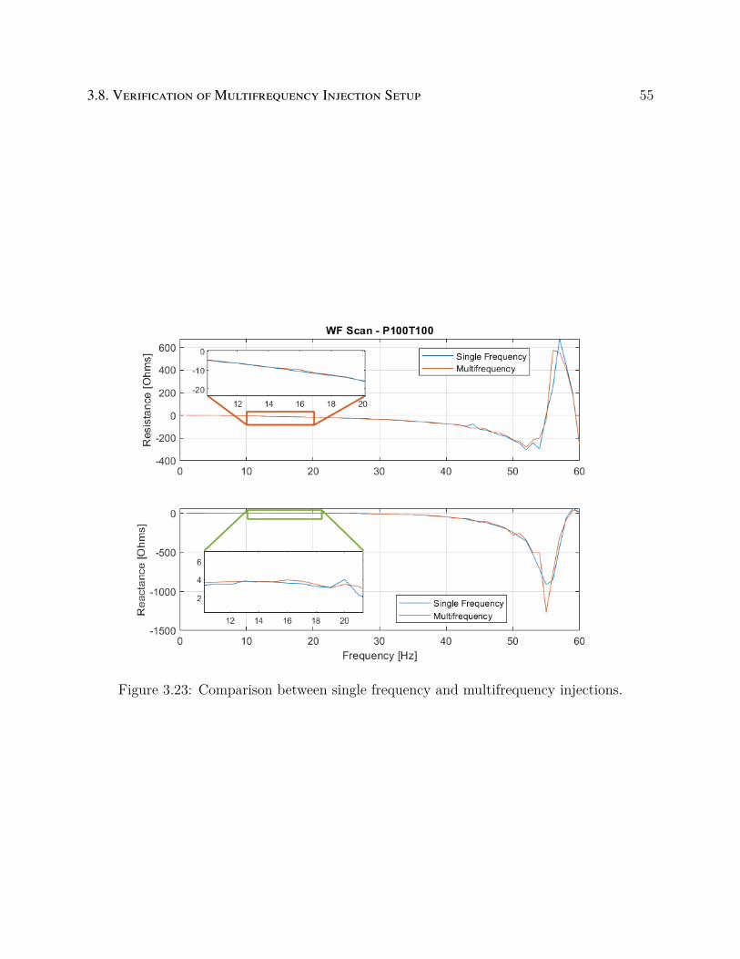
3.8. VERIFICATION OF MULTIFREQUENCY INJECTION SETUP 55
Figure 3.23: Comparison between single frequency and multifrequency injections.

Chapter 4
Frequency Scan Based Mitigation
Approach of SSCI
4.1 Parallel Multifrequency Injection Scan
Using the multifrequency injection method described in Section 3.7, the studied system has
been modified to adjust for a parallel scan configuration, as shown in Figure 4.1.
Figure 4.1: Parallel scan setup in PSCAD/EMTDC.
Where the parallel scan box consists of three main parts, the first being the harmonic
generation part which has three harmonic injection blocks, each for a single phase, the
harmonic injection part with three single phase current sources that take their output from
their respective harmonic injection block and the parallel scan enabler that scans the entire
system as shown in Figure 4.2. The harmonic generation blocks takes the magnitudes and
phase angles from a .txt file that is generated using Python to match the optimized injection
56

4.1. PARALLEL MULTIFREQUENCY INJECTION SCAN 57
Figure 4.2: Components of parallel scan box.
signal.
Using the scan multimeter that is highlighted in red in Figure 4.1, and by having all of the
WF impedances obtained in Chapter 3 in a look-up table, the system impedance can be
calculated as follows:
Zscan =ZWF × Zgrid
ZWF + Zgrid(4.1)
∴ Zgrid =Zscan × ZWF
ZWF − Zscan(4.2)
The results of using eqn 4.2 is shown in Figure 4.3 which was done using MATLAB post
processing of the scan current and voltage and also by using PSCAD/EMTDC FFT blocks in
comparison to the theoretical values. PSCAD values are the closest to match the theoretical
values.

58 CHAPTER 4. FREQUENCY SCAN BASED MITIGATION APPROACH OF SSCI
0 10 20 30 40 50 60-5
0
5
10
Res
ista
nce
[Ohm
s]
0 10 20 30 40 50 60Frequency [Hz]
-5
0
5
10
Rea
ctan
ce [
Ohm
s]
MATLABPSCADTheoretical
Figure 4.3: System impedance using parallel scan.
The amplitude of the current injection must be low enough to ensure that the parallel scan
does not interfere with the steady state operating point, therefore the amplitude was chosen
to be 1% of the steady state current value which amounts to 0.002 kA in this case. The
disruption caused due to this injection is minimal and is shown in Figure 4.4.

4.1. PARALLEL MULTIFREQUENCY INJECTION SCAN 59
Figure 4.4: Parallel scan impact on steady-state operation.
The parallel scan was enabled at time = 4 s, depicted with the black dashed line in Figure
4.4. The disruption in the output power is less than 1% with almost negligible effect on the
RMS voltage.

60 CHAPTER 4. FREQUENCY SCAN BASED MITIGATION APPROACH OF SSCI
4.2 Mitigation of SSCI Approach
The approach to mitigate SSCI using the on-line frequency scan goes as the following:
1. Once SSCI is detected, the proportional gains of the dq-axis is reduced to very low
values to prevent oscillations from growing exponentially.
2. Parallel scan is enabled to identify grid impedance.
3. Grid impedance is combined with WF impedance to obtain the overall system impedance.
4. External or internal parameters are changed to mitigate the risk of SSCI.
In the simulated system in PSCAD, the following takes place:
1. The system is started with Line #2 in service.
2. It takes 3 seconds for the WF to stabilize and reach steady-state.
3. At time = 5 s, Line #2 trips.
4. Proportional gains are reduced.
5. Parallel scan is enabled.
6. Parallel scan results are processed.
7. Parameters are changed to mitigate SSCI.
The following flowchart depicts the methodology.

4.2. MITIGATION OF SSCI APPROACH 61
Steady-State
Detection of SSCI
Immediate Change of Parameters
Parallel Scan
Change of Parameters
Mitigation of SSCI Turn off WF
Steady-State
yes
no
Figure 4.5: Flowchart of SSCI mitigation approach.
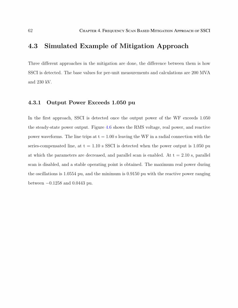
62 CHAPTER 4. FREQUENCY SCAN BASED MITIGATION APPROACH OF SSCI
4.3 Simulated Example of Mitigation Approach
Three different approaches in the mitigation are done, the difference between them is how
SSCI is detected. The base values for per-unit measurements and calculations are 200 MVA
and 230 kV.
4.3.1 Output Power Exceeds 1.050 pu
In the first approach, SSCI is detected once the output power of the WF exceeds 1.050
the steady-state power output. Figure 4.6 shows the RMS voltage, real power, and reactive
power waveforms. The line trips at t = 1.00 s leaving the WF in a radial connection with the
series-compensated line, at t = 1.10 s SSCI is detected when the power output is 1.050 pu
at which the parameters are decreased, and parallel scan is enabled. At t = 2.10 s, parallel
scan is disabled, and a stable operating point is obtained. The maximum real power during
the oscillations is 1.0554 pu, and the minimum is 0.9150 pu with the reactive power ranging
between −0.1258 and 0.0443 pu.

4.3. SIMULATED EXAMPLE OF MITIGATION APPROACH 63
Figure 4.6: RMS voltage, real power, and reactive power waveforms for when output powerexceeds 1.050 pu. (black-dashed line is when line #2 trips, yellow-dashed line is when SSCIis detected, and yellow straight line is when a stable operating point is found).
4.3.2 Output Power Exceeds 1.025 pu
In the second approach, SSCI is detected once the output power of the WF exceeds 1.025
the steady-state power output. Figure 4.7 shows the RMS voltage, real power, and reactive
power waveforms. The line trips at t = 1.00 s, leaving the WF in a radial connection with
the series-compensated line, at t = 1.06 s SSCI is detected when the power output is 1.025 pu
at which the parameters are decreased, and parallel scan is enabled. At t = 2.06 s, parallel
scan is disabled, and a stable operating point is obtained. The maximum real power during
the oscillations is 1.0487 pu, and the minimum is 0.9467 pu with the reactive power ranging
between −0.0798 and 0.0191 pu.

64 CHAPTER 4. FREQUENCY SCAN BASED MITIGATION APPROACH OF SSCI
Figure 4.7: RMS voltage, real power, and reactive power waveforms when output powerexceeds 1.025 pu. (black-dashed line is when line #2 trips, yellow-dashed line is when SSCIis detected, and yellow straight line is when a stable operating point is found).
4.3.3 Access to External Signal
In the third approach, it is assumed that the WF has access to the tripping signal of the
CB associated with Line #2. Figure 4.8 shows the RMS voltage, real power, and reactive
power waveforms. The line trips at t = 1.00 s, leaving the WF in a radial connection with
the series-compensated line, at t = 1.00 s, SSCI is detected when the CB is open at which
the parameters are decreased, and parallel scan is enabled. At t = 2.00 s, parallel scan is
disabled, and a stable operating point is obtained. The maximum real power during the
oscillations is 1.0464 pu and the minimum is 0.9536 pu with the reactive power ranging
between −0.0447 and −0.0126 pu.
The normal operation without any mitigation approach yields an undamped oscillation that

4.3. SIMULATED EXAMPLE OF MITIGATION APPROACH 65
Figure 4.8: RMS voltage, real power, and reactive power waveforms with access to externalsignal. (black-dashed line is when line #2 trips, yellow-dashed line is when SSCI is detected,and yellow straight line is when a stable operating point is found).
grows to 4.29 pu before the rotor stops spinning due to growing subsynchronous currents.
Figure 4.9 shows the real power output in the normal operation without any migitation in
comparison to three mitigation approaches. Oscillations grow to 2.5 pu in 0.5 s without any
mitigation.
4.3.4 Discussion
SSCI is mitigated in all of the three approaches; (i) output power exceeds 1.050 pu, (ii)
output power exceeds 1.025 pu, and (iii) access to external signal. Real power oscillation
is the most significant in the first approach (output power exceeds 1.050 pu), and the least
significant in the third approach (access to external signal). Once a stable operating point
is obtained, in all of the previously mentioned approaches, the real power oscillation is less

66 CHAPTER 4. FREQUENCY SCAN BASED MITIGATION APPROACH OF SSCI
Figure 4.9: Comparison between no mitigation operation and the three mitigation ap-proaches.
than 0.70%. Reactive power oscillations are minimized and the RMS voltage ranges between
0.998 pu and 1.002 pu. In the normal operation without any mitigation approach, the output
power grows to 2 pu in less than 0.30 s. This can either lead to excessive damage in WTs or
to the disconnection of the WF, both of these scenarios lead to an undesired disruption of
service.
Table 4.1: Comparison between the three mitigation approaches
Approach Real Power Range [pu] Reactive Power Range[pu]
Output power exceeds 1.050 pu 0.9150 to 1.0554 −0.1258 to 0.0443Output power exceeds 1.025 pu 0.9467 to 1.0487 −0.0798 to 0.0191Access to external signal 0.9536 to 1.0464 −0.0447 to −0.0126

Chapter 5
Contributions and Future Work
The contributions of this thesis are as follows:
• Discussing the various types of SSOs including SSR, SSTI, TI, and IGE.
• Explaining SSCI and the mechanism of interaction between series compensation and
Type-3 wind turbines.
• Comparing different methods of frequency scans and proposing an optimization prob-
lem to reduce peak voltage.
• Usage of on-line parallel harmonic injection, along with frequency scan to mitigate
SSCI.
Whereas in the future, this work can be built on in any one of the following ways:
• Investigating the effect of other parameters and their influence on the impedance of
the WF.
• Modifying the GSC controller to inject harmonics instead of using a parallel scan
approach.
• Obtaining the impedance of the WF without having to use a look-up table through
parametric equations.
67

Bibliography
[1] H. Haes Alhelou, M. E. Hamedani-Golshan, T. C. Njenda, and P. Siano, “A survey on
power system blackout and cascading events: Research motivations and challenges,”
Energies, vol. 12, no. 4, p. 682, 2019.
[2] Y.-K. Wu, S. M. Chang, and Y.-L. Hu, “Literature review of power system blackouts,”
Energy Procedia, vol. 141, pp. 428–431, 2017.
[3] T. I. R. E. A. (IRENA), “Renewable Capacity Statistics 2021,” The International Re-
newable Energy Agency (IRENA), Abu Dhabi, Tech. Rep.
[4] IEA, “World Energy Outlook 2020,” IEA, Paris, Tech. Rep., 2020. [Online]. Available:
https://www.iea.org/reports/world-energy-outlook-2020
[5] P. Sadorsky, “Wind energy for sustainable development: Driving factors and future
outlook,” Journal of Cleaner Production, vol. 289, p. 125779, 2021.
[6] H. Abu-Rub, M. Malinowski, and K. Al-Haddad, Power electronics for renewable energy
systems, transportation and industrial applications. John Wiley & Sons, 2014.
[7] E. Muljadi, Y. C. Zhang, V. Gevorgian, and D. Kosterev, “Understanding dynamic
model validation of a wind turbine generator and a wind power plant,” in 2016 IEEE
Energy Conversion Congress and Exposition (ECCE). IEEE, 2016, pp. 1–5.
[8] “Global Wind Report 2021,” Mar. 2021. [Online]. Available: https://gwec.net/
global-wind-report-2021/
[9] L. Fan, R. Kavasseri, Z. L. Miao, and C. Zhu, “Modeling of dfig-based wind farms for ssr
analysis,” IEEE Transactions on Power Delivery, vol. 25, no. 4, pp. 2073–2082, 2010.
68

BIBLIOGRAPHY 69
[10] J. Garcia-Gonzalez, R. M. R. de la Muela, L. M. Santos, and A. M. Gonzalez, “Stochas-
tic joint optimization of wind generation and pumped-storage units in an electricity
market,” IEEE Transactions on Power Systems, vol. 23, no. 2, pp. 460–468, 2008.
[11] V. Virulkar and G. Gotmare, “Sub-synchronous resonance in series compensated wind
farm: A review,” Renewable and Sustainable Energy Reviews, vol. 55, pp. 1010–1029,
2016.
[12] R. K. Varma and A. Moharana, “Ssr in double-cage induction generator-based wind
farm connected to series-compensated transmission line,” IEEE transactions on power
systems, vol. 28, no. 3, pp. 2573–2583, 2013.
[13] I. S. R. W. Group et al., “Terms, definitions and symbols for subsynchronous oscil-
lations,” IEEE Transactions on Power Apparatus and Systems, vol. 104, no. 6, pp.
1326–1334, 1985.
[14] ——, “Proposed terms and definitions for subsynchronous oscillations,” IEEE Transac-
tions on Power Apparatus and Systems, vol. 99, no. 2, pp. 506–511, 1980.
[15] J. Butler and C. Concordia, “Analysis of series capacitor application problems,” Elec-
trical Engineering, vol. 56, no. 8, pp. 975–988, 1937.
[16] D. Walker, C. Bowler, R. Jackson, and D. Hodges, “Results of subsynchronous resonance
test at mohave,” IEEE Transactions on Power Apparatus and Systems, vol. 94, no. 5,
pp. 1878–1889, 1975.
[17] J. W. Ballance and S. Goldberg, “Subsynchronous resonance in series compensated
transmission lines,” IEEE Transactions on Power Apparatus and Systems, no. 5, pp.
1649–1658, 1973.

70 BIBLIOGRAPHY
[18] J. Daniel, W. Wong, G. Ingeström, and J. Sjöberg, “Subsynchronous phenomena and
wind turbine generators,” in PES T&D 2012. IEEE, 2012, pp. 1–6.
[19] “Reader’s guide to subsynchronous resonance,” IEEE Transactions on Power Systems,
vol. 7, no. 1, pp. 150–157, 1992.
[20] R. N. Damas, Y. Son, M. Yoon, S.-Y. Kim, and S. Choi, “Subsynchronous Oscillation
and Advanced Analysis: A Review,” IEEE Access, vol. 8, pp. 224 020–224 032, 2020.
[21] A. E. Leon and J. A. Solsona, “Sub-Synchronous Interaction Damping Control for DFIG
Wind Turbines,” IEEE Transactions on Power Systems, vol. 30, no. 1, pp. 419–428, Jan.
2015.
[22] M. Bahrman, E. Larsen, R. Piwko, and H. Patel, “Experience with hvdc-turbine-
generator torsional interaction at square butte,” IEEE Transactions on Power Apparatus
and Systems, no. 3, pp. 966–975, 1980.
[23] A. Mulawarman and P. Mysore, “Detection of undamped sub-synchronous oscillations
of wind generators with series compensated lines,” in Minnesota Power Systems Con-
ference, 2011.
[24] H. Ma, P. Brogan, K. Jensen, and R. Nelson, “Sub-synchronous control interaction
studies between full-converter wind turbines and series-compensated ac transmission
lines,” in 2012 IEEE Power and Energy Society General Meeting. IEEE, 2012, pp. 1–5.
[25] J. R. Ramamurthy and L. J. Bohmann, “Wind Plant Interaction in a 345-kV Series-
compensated Power System—Electromagnetic Transient Program Modeling and Event
Analysis,” Electric Power Components and Systems, vol. 44, no. 15, pp. 1745–1756,
2016.

BIBLIOGRAPHY 71
[26] G. Irwin, “Sub-synchronous interactions with wind turbines,” in Technical Conference-
CREZ System Design and Operation, 2010.
[27] W. Wong and J. Daniel, ABB presentation on CREZ Reactive Study-ERCOT RPG
Meeting. March, 2010.
[28] S.-H. Huang, J. Schmall, J. Conto, J. Adams, Y. Zhang, and C. Carter, “Voltage control
challenges on weak grids with high penetration of wind generation: ERCOT experience,”
in 2012 IEEE Power and Energy Society General Meeting, Jul. 2012, pp. 1–7.
[29] S. Huang and Y. Gong, “South Texas SSR,” in Proc. ERCOT Rel. Oper Meeting, 2018.
[30] X. Xie, X. Zhang, H. Liu, H. Liu, Y. Li, and C. Zhang, “Characteristic Analysis of
Subsynchronous Resonance in Practical Wind Farms Connected to Series-Compensated
Transmissions,” IEEE Transactions on Energy Conversion, vol. 32, no. 3, pp. 1117–
1126, Sep. 2017.
[31] H. Jiang, S. Ma, R. Song, and Z. Xiang, “Analysis on subsynchronous oscillation stabil-
ity for large scale offshore wind integration,” Energy Reports, vol. 6, pp. 189–195, Dec.
2020.
[32] Analytic Methods for Power Systems Committee (AMPS), “Wind Energy Systems
Sub-synchronous Oscillations: Events and Modeling,” IEEE Power & Energy Society,
Tech. Rep. TR-80, Jul. 2020. [Online]. Available: https://resourcecenter.ieee-pes.org/
publications/technical-reports/PES_TP_TR80_AMPS_WSSO_070920.html
[33] L. Fan and Z. Miao, “An Explanation of Oscillations Due to Wind Power Plants Weak
Grid Interconnection,” IEEE Transactions on Sustainable Energy, vol. 9, no. 1, pp.
488–490, 2018.

72 BIBLIOGRAPHY
[34] J. Shair, X. Xie, W. Liu, X. Li, and H. Li, “Modeling and stability analysis methods
for investigating subsynchronous control interaction in large-scale wind power systems,”
Renewable and Sustainable Energy Reviews, vol. 135, p. 110420, 2021.
[35] J. Shair, X. Xie, and G. Yan, “Mitigating subsynchronous control interaction in wind
power systems: Existing techniques and open challenges,” Renewable and Sustainable
Energy Reviews, vol. 108, pp. 330–346, 2019.
[36] L. Wang, X. Xie, Q. Jiang, H. Liu, Y. Li, and H. Liu, “Investigation of SSR in Practical
DFIG-Based Wind Farms Connected to a Series-Compensated Power System,” IEEE
Transactions on Power Systems, vol. 30, no. 5, pp. 2772–2779, Sep. 2015.
[37] L. Fan, C. Zhu, Z. Miao, and M. Hu, “Modal Analysis of a DFIG-Based Wind Farm
Interfaced With a Series Compensated Network,” IEEE Transactions on Energy Con-
version, vol. 26, no. 4, pp. 1010–1020, 2011.
[38] F. Mei and B. Pal, “Modelling and small-signal analysis of a grid connected doubly-fed
induction generator,” in IEEE Power Engineering Society General Meeting, 2005. San
Francisco, CA, USA: IEEE, 2005, pp. 1503–1510.
[39] H. A. Mohammadpour and E. Santi, “Sub-synchronous resonance analysis in DFIG-
based wind farms: Definitions and problem identification — Part I,” in 2014
IEEE Energy Conversion Congress and Exposition (ECCE). Pittsburgh, PA, USA:
IEEE, 2014, pp. 812–819.
[40] B. Badrzadeh, M. Sahni, Y. Zhou, D. Muthumuni, and A. Gole, “General Methodology
for Analysis of Sub-Synchronous Interaction in Wind Power Plants,” IEEE Transactions
on Power Systems, vol. 28, no. 2, pp. 1858–1869, 2013.

BIBLIOGRAPHY 73
[41] M. Sahni, D. Muthumuni, B. Badrzadeh, A. Gole, and A. Kulkarni, “Advanced screen-
ing techniques for Sub-Synchronous Interaction in wind farms,” in PES T&D 2012.
Orlando, FL, USA: IEEE, 2012, pp. 1–9.
[42] M. Ghafouri, U. Karaagac, H. Karimi, S. Jensen, J. Mahseredjian, and S. O. Faried,
“An LQR Controller for Damping of Subsynchronous Interaction in DFIG-Based Wind
Farms,” IEEE Transactions on Power Systems, vol. 32, no. 6, pp. 4934–4942, 2017.
[43] H. A. Mohammadpour and E. Santi, “SSR Damping Controller Design and Optimal
Placement in Rotor-Side and Grid-Side Converters of Series-Compensated DFIG-Based
Wind Farm,” IEEE Transactions on Sustainable Energy, vol. 6, no. 2, pp. 388–399,
2015.
[44] X. Zhang, X. Xie, H. Liu, and Y. Li, “Robust subsynchronous damping control to sta-
bilise SSR in series‐compensated wind power systems,” IET Generation, Transmission
& Distribution, vol. 13, no. 3, pp. 337–344, 2019.
[45] J. Shair, X. Xie, Y. Li, and V. Terzija, “Hardware-in-the-Loop and Field Validation
of a Rotor-Side Subsynchronous Damping Controller for a Series Compensated DFIG
System,” IEEE Transactions on Power Delivery, vol. 36, no. 2, pp. 698–709, 2021.
[46] X. Zhang, X. Xie, J. Shair, H. Liu, Y. Li, and Y. Li, “A Grid-Side Subsynchronous
Damping Controller to Mitigate Unstable SSCI and Its Hardware-in-the-loop Tests,”
IEEE Transactions on Sustainable Energy, vol. 11, no. 3, pp. 1548–1558, 2020.
[47] R. D. Middlebrook, “Improved-accuracy phase angle measurement,” International Jour-
nal of Electronics, vol. 40, no. 1, pp. 1–4, 1976.
[48] Jian Sun, “Small-Signal Methods for AC Distributed Power Systems–A Review,” IEEE
Transactions on Power Electronics, vol. 24, no. 11, pp. 2545–2554, Nov. 2009.

74 BIBLIOGRAPHY
[49] L. Harnefors, M. Bongiorno, and S. Lundberg, “Input-Admittance Calculation and
Shaping for Controlled Voltage-Source Converters,” IEEE Transactions on Industrial
Electronics, vol. 54, no. 6, pp. 3323–3334, 2007.
[50] L. Fan and Z. Miao, “Nyquist-Stability-Criterion-Based SSR Explanation for Type-3
Wind Generators,” IEEE Transactions on Energy Conversion, vol. 27, no. 3, pp. 807–
809, 2012.
[51] H. Liu, X. Xie, C. Zhang, Y. Li, H. Liu, and Y. Hu, “Quantitative SSR Analysis of
Series-Compensated DFIG-Based Wind Farms Using Aggregated RLC Circuit Model,”
IEEE Transactions on Power Systems, vol. 32, no. 1, pp. 474–483, 2017.
[52] Z. Miao, “Impedance-Model-Based SSR Analysis for Type 3 Wind Generator and Series-
Compensated Network,” IEEE Transactions on Energy Conversion, vol. 27, no. 4, pp.
984–991, 2012.
[53] P. M. Anderson, B. L. Agrawal, and J. E. Van Ness, Subsynchronous resonance in power
systems. John Wiley & Sons, 1999, vol. 9.
[54] H. Liu, X. Xie, and W. Liu, “An oscillatory stability criterion based on the unified dq-
frame impedance network model for power systems with high-penetration renewables,”
IEEE Transactions on Power Systems, vol. 33, no. 3, pp. 3472–3485, 2018.
[55] C. Zhu, M. Hu, and Z. Wu, “Parameters impact on the performance of a double-fed
induction generator-based wind turbine for subsynchronous resonance control,” IET
Renewable Power Generation, vol. 6, no. 2, pp. 92–98, 2012.
[56] L. Zhang, L. Harnefors, and H.-P. Nee, “Interconnection of two very weak ac systems
by vsc-hvdc links using power-synchronization control,” IEEE transactions on power
systems, vol. 26, no. 1, pp. 344–355, 2010.

BIBLIOGRAPHY 75
[57] R. K. Varma, S. Auddy, and Y. Semsedini, “Mitigation of subsynchronous resonance in
a series-compensated wind farm using facts controllers,” IEEE transactions on power
delivery, vol. 23, no. 3, pp. 1645–1654, 2008.
[58] M. S. El-Moursi, “Mitigating subsynchronous resonance and damping power system
oscillation in a series compensated wind park using a novel static synchronous series
compensator control algorithm,” Wind Energy, vol. 15, no. 3, pp. 363–377, 2012.
[59] Z. An, C. Shen, Z. Zheng, F. Liu, X. Chang, and W. Wei, “Scenario-based analysis
and probability assessment of sub-synchronous oscillation caused by wind farms with
direct-driven wind generators,” Journal of Modern Power Systems and Clean Energy,
vol. 7, no. 2, pp. 243–253, 2019.
[60] W. Lasher, C. Carter, J. Daniel, D. Martin, W. Wong, and R. Koessler, “Analysis of
reactive compensation design for the competitive renewable energy zones transmission
plan in texas,” 2010.
[61] X. Xie, W. Liu, H. Liu, Y. Du, and Y. Li, “A system-wide protection against unstable
ssci in series-compensated wind power systems,” IEEE Transactions on Power Delivery,
vol. 33, no. 6, pp. 3095–3104, 2018.
[62] L. Fan and Z. Miao, “Mitigating ssr using dfig-based wind generation,” IEEE Transac-
tions on Sustainable Energy, vol. 3, no. 3, pp. 349–358, 2012.
[63] H. Ghaffarzdeh and A. Mehrizi-Sani, “Mitigation of subsynchronous resonance induced
by a type iii wind system,” IEEE Transactions on Sustainable Energy, vol. 11, no. 3,
pp. 1717–1727, 2019.
[64] H. A. Mohammadpour, A. Ghaderi, H. Mohammadpour, and E. Santi, “Ssr damping

76 BIBLIOGRAPHY
in wind farms using observed-state feedback control of dfig converters,” Electric Power
Systems Research, vol. 123, pp. 57–66, 2015.
[65] P.-H. Huang, M. S. El Moursi, W. Xiao, and J. L. Kirtley, “Subsynchronous resonance
mitigation for series-compensated dfig-based wind farm by using two-degree-of-freedom
control strategy,” IEEE Transactions on Power Systems, vol. 30, no. 3, pp. 1442–1454,
2014.
[66] J. Adams, C. Carter, and S.-H. Huang, “Ercot experience with sub-synchronous control
interaction and proposed remediation,” in PES T&D 2012. IEEE, 2012, pp. 1–5.
[67] A. Testa and R. Langella, “Power system subharmonics,” in IEEE Power Engineering
Society General Meeting, 2005. IEEE, 2005, pp. 1922–1927.
[68] D. Kidd and P. Hassink, “Transmission operator perspective of sub-synchronous inter-
action,” in PES T&D 2012. IEEE, 2012, pp. 1–3.
[69] L. C. Gross et al., “Sub-synchronous grid conditions: New event new problem and new
solutions,” in Proc. Western Protective Relay Conf, vol. 2010, 2010, pp. 1–19.
[70] X. Jiang and A. Gole, “A frequency scanning method for the identification of harmonic
instabilities in hvdc systems,” IEEE Transactions on Power Delivery, vol. 10, no. 4, pp.
1875–1881, 1995.
[71] “Second benchmark model for computer simulation of subsynchronous resonance,” IEEE
Transactions on Power Apparatus and Systems, vol. PAS-104, no. 5, pp. 1057–1066,
1985.
[72] A. Miller, E. Muljadi, and D. Zinger, “A variable speed wind turbine power control,”
IEEE Transactions on Energy Conversion, vol. 12, no. 2, pp. 181–186, 1997.

BIBLIOGRAPHY 77
[73] A. Shafiu, O. Anaya-Lara, G. Bathurst, and N. Jenkins, “Aggregated wind turbine
models for power system dynamic studies,” Wind Engineering, vol. 30, no. 3, pp. 171–
185, 2006.
[74] W. H. Kersting, Distribution system modeling and analysis, fourth edition ed. Boca
Raton: CRC Press, Taylor & Francis Group, CRC Press is an imprint of the Taylor &
Francis Group, an informa business, 2018.
[75] E. Muljadi, C. Butterfield, A. Ellis, J. Mechenbier, J. Hochheimer, R. Young, N. Miller,
R. Delmerico, R. Zavadil, and J. Smith, “Equivalencing the collector system of a large
wind power plant,” in 2006 IEEE Power Engineering Society General Meeting, 2006,
pp. 9 pp.–.
[76] E. Muljadi, S. Pasupulati, A. Ellis, and D. Kosterov, “Method of equivalencing for a
large wind power plant with multiple turbine representation,” in 2008 IEEE power and
energy society general meeting-conversion and delivery of electrical energy in the 21st
century. IEEE, 2008, pp. 1–9.
[77] G. Abad, J. Lopez, M. Rodriguez, L. Marroyo, and G. Iwanski, Doubly fed induction
machine: modeling and control for wind energy generation. John Wiley & Sons, 2011,
vol. 85.
[78] K. Gu, F. Wu, and X.-P. Zhang, “Sub-synchronous interactions in power systems with
wind turbines: a review,” IET Renewable Power Generation, vol. 13, no. 1, pp. 4–15,
2019.
[79] G. R. Slemon, “Modelling of induction machines for electric drives,” IEEE Transactions
on Industry Applications, vol. 25, no. 6, pp. 1126–1131, 1989.

78 BIBLIOGRAPHY
[80] O. Semiconductor, “Reading ON semiconductor IGBT datasheets,” https://www.
onsemi.com/pub/Collateral/AND9068-D.PDF, accessed: 2021-05-31.
[81] A. Kulkarni, M. Das, and A. Gole, “Frequency scanning analysis of statcom-network
interactions,” in 2016 IEEE 6th International Conference on Power Systems (ICPS).
IEEE, 2016, pp. 1–6.
[82] R. Pintelon and J. Schoukens, System identification: a frequency domain approach.
John Wiley & Sons, 2012.
[83] I. B. M. Matsuo, F. Salehi, L. Zhao, Y. Zhou, and W.-J. Lee, “Optimized frequency
scanning of nonlinear devices applied to subsynchronous resonance screening,” IEEE
Transactions on Industry Applications, vol. 56, no. 3, pp. 2281–2291, 2020.

Appendices
79

Appendix A
System Scan Results
The full results for the system scan will be listed in this appendix.
A.1 Variation of q-axis Proportional Gain
In this section, system scan results under various proportional gains for the q-axis inner
control loop will be listed in Figures A.1 - A.20.
80

A.1. VARIATION OF Q-AXIS PROPORTIONAL GAIN 81
Figure A.1: System scan for Kpd = 2.00 and Kpq = 0.50.
Figure A.2: System scan for Kpd = 2.00 and Kpq = 1.00.

82 APPENDIX A. SYSTEM SCAN RESULTS
Figure A.3: System scan for Kpd = 2.00 and Kpq = 1.50.
Figure A.4: System scan for Kpd = 2.00 and Kpq = 2.00.

A.1. VARIATION OF Q-AXIS PROPORTIONAL GAIN 83
Figure A.5: System scan for Kpd = 2.00 and Kpq = 2.50.
Figure A.6: System scan for Kpd = 2.00 and Kpq = 3.00.

84 APPENDIX A. SYSTEM SCAN RESULTS
Figure A.7: System scan for Kpd = 2.00 and Kpq = 3.50.
Figure A.8: System scan for Kpd = 2.00 and Kpq = 4.00.

A.1. VARIATION OF Q-AXIS PROPORTIONAL GAIN 85
Figure A.9: System scan for Kpd = 2.00 and Kpq = 4.50.
Figure A.10: System scan for Kpd = 2.00 and Kpq = 5.00.
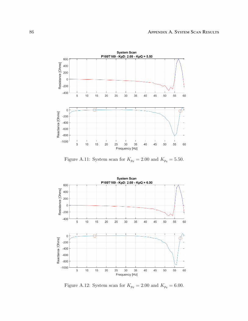
86 APPENDIX A. SYSTEM SCAN RESULTS
Figure A.11: System scan for Kpd = 2.00 and Kpq = 5.50.
Figure A.12: System scan for Kpd = 2.00 and Kpq = 6.00.
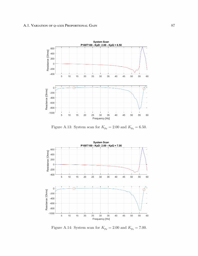
A.1. VARIATION OF Q-AXIS PROPORTIONAL GAIN 87
Figure A.13: System scan for Kpd = 2.00 and Kpq = 6.50.
Figure A.14: System scan for Kpd = 2.00 and Kpq = 7.00.

88 APPENDIX A. SYSTEM SCAN RESULTS
Figure A.15: System scan for Kpd = 2.00 and Kpq = 7.50.
Figure A.16: System scan for Kpd = 2.00 and Kpq = 8.00.

A.1. VARIATION OF Q-AXIS PROPORTIONAL GAIN 89
Figure A.17: System scan for Kpd = 2.00 and Kpq = 8.50.
Figure A.18: System scan for Kpd = 2.00 and Kpq = 9.00.

90 APPENDIX A. SYSTEM SCAN RESULTS
Figure A.19: System scan for Kpd = 2.00 and Kpq = 9.50.
Figure A.20: System scan for Kpd = 2.00 and Kpq = 10.00.

A.2. VARIATION OF D-AXIS PROPORTIONAL GAIN 91
Figure A.21: System scan for Kpd = 0.50 and Kpq = 2.00.
A.2 Variation of d-axis Proportional Gain
In this section, system scan results under various proportional gains for the d-axis inner
control loop will be listed in Figures A.21 - A.39.

92 APPENDIX A. SYSTEM SCAN RESULTS
Figure A.22: System scan for Kpd = 1.00 and Kpq = 2.00.
Figure A.23: System scan for Kpd = 1.50 and Kpq = 2.00.

A.2. VARIATION OF D-AXIS PROPORTIONAL GAIN 93
Figure A.24: System scan for Kpd = 2.50 and Kpq = 2.00.
Figure A.25: System scan for Kpd = 3.00 and Kpq = 2.00.

94 APPENDIX A. SYSTEM SCAN RESULTS
Figure A.26: System scan for Kpd = 3.50 and Kpq = 2.00.
Figure A.27: System scan for Kpd = 4.00 and Kpq = 2.00.

A.2. VARIATION OF D-AXIS PROPORTIONAL GAIN 95
Figure A.28: System scan for Kpd = 4.50 and Kpq = 2.00.
Figure A.29: System scan for Kpd = 5.00 and Kpq = 2.00.
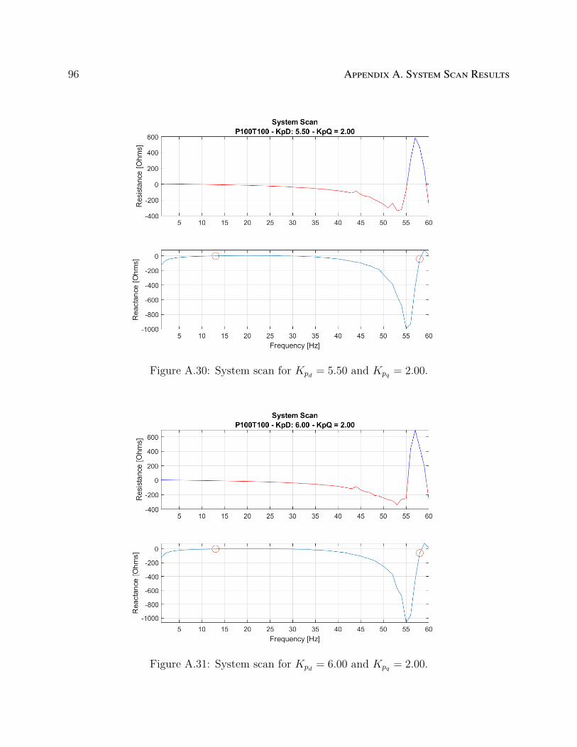
96 APPENDIX A. SYSTEM SCAN RESULTS
Figure A.30: System scan for Kpd = 5.50 and Kpq = 2.00.
Figure A.31: System scan for Kpd = 6.00 and Kpq = 2.00.

A.2. VARIATION OF D-AXIS PROPORTIONAL GAIN 97
Figure A.32: System scan for Kpd = 6.50 and Kpq = 2.00.
Figure A.33: System scan for Kpd = 7.00 and Kpq = 2.00.

98 APPENDIX A. SYSTEM SCAN RESULTS
Figure A.34: System scan for Kpd = 7.50 and Kpq = 2.00.
Figure A.35: System scan for Kpd = 8.00 and Kpq = 2.00.

A.2. VARIATION OF D-AXIS PROPORTIONAL GAIN 99
Figure A.36: System scan for Kpd = 8.50 and Kpq = 2.00
Figure A.37: System scan for Kpd = 9.00 and Kpq = 2.00.

100 APPENDIX A. SYSTEM SCAN RESULTS
Figure A.38: System scan for Kpd = 9.50 and Kpq = 2.00.
Figure A.39: System scan for Kpd = 10.00 and Kpq = 2.00.
A.3. VARIATION OF dq-AXIS PROPORTIONAL GAIN 101
A.3 Variation of dq-axis Proportional Gain
In this section, system scan results under various proportional gains for the dq-axis inner
control loops will be listed in Figures A.40 - A.58.

102 APPENDIX A. SYSTEM SCAN RESULTS
Figure A.40: System scan for Kpd = 0.50 and Kpq = 0.50.
Figure A.41: System scan for Kpd = 1.00 and Kpq = 1.00.

A.3. VARIATION OF dq-AXIS PROPORTIONAL GAIN 103
Figure A.42: System scan for Kpd = 1.50 and Kpq = 1.50.
Figure A.43: System scan for Kpd = 2.50 and Kpq = 2.50.

104 APPENDIX A. SYSTEM SCAN RESULTS
Figure A.44: System scan for Kpd = 3.00 and Kpq = 3.00.
Figure A.45: System scan for Kpd = 3.50 and Kpq = 3.50.
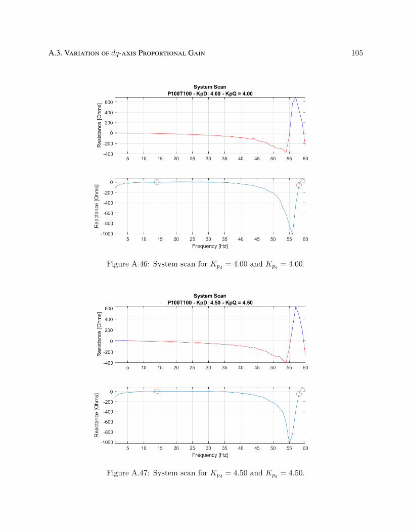
A.3. VARIATION OF dq-AXIS PROPORTIONAL GAIN 105
Figure A.46: System scan for Kpd = 4.00 and Kpq = 4.00.
Figure A.47: System scan for Kpd = 4.50 and Kpq = 4.50.

106 APPENDIX A. SYSTEM SCAN RESULTS
Figure A.48: System scan for Kpd = 5.00 and Kpq = 5.00.
Figure A.49: System scan for Kpd = 5.50 and Kpq = 5.50.

A.3. VARIATION OF dq-AXIS PROPORTIONAL GAIN 107
Figure A.50: System scan for Kpd = 6.00 and Kpq = 6.00.
Figure A.51: System scan for Kpd = 6.50 and Kpq = 6.50.

108 APPENDIX A. SYSTEM SCAN RESULTS
Figure A.52: System scan for Kpd = 7.00 and Kpq = 7.00.
Figure A.53: System scan for Kpd = 7.50 and Kpq = 7.50.

A.3. VARIATION OF dq-AXIS PROPORTIONAL GAIN 109
Figure A.54: System scan for Kpd = 8.00 and Kpq = 8.00.
Figure A.55: System scan for Kpd = 8.50 and Kpq = 8.50.

110 APPENDIX A. SYSTEM SCAN RESULTS
Figure A.56: System scan for Kpd = 9.00 and Kpq = 9.00.
Figure A.57: System scan for Kpd = 9.50 and Kpq = 9.50.

A.3. VARIATION OF dq-AXIS PROPORTIONAL GAIN 111
Figure A.58: System scan for Kpd = 10.00 and Kpq = 10.00.

112 APPENDIX A. SYSTEM SCAN RESULTS
A.4 Variation of Online Turbines
In this section, system scan results under various number of online turbines will be listed in
Figures A.59 - A.62.
Figure A.59: System scan for 100% online turbines.

A.4. VARIATION OF ONLINE TURBINES 113
Figure A.60: System scan for 50% online turbines.
Figure A.61: System scan for 25% online turbines.

114 APPENDIX A. SYSTEM SCAN RESULTS
Figure A.62: System scan for 10% online turbines.
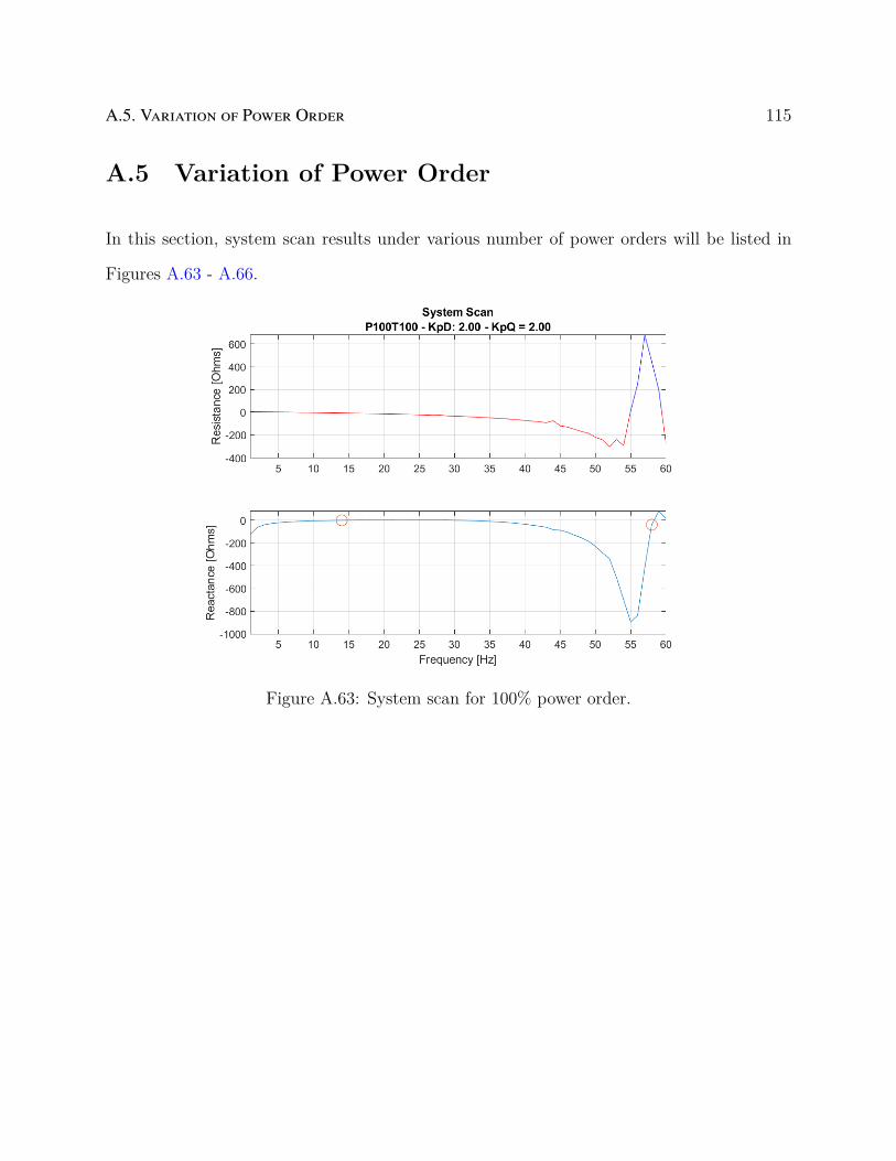
A.5. VARIATION OF POWER ORDER 115
A.5 Variation of Power Order
In this section, system scan results under various number of power orders will be listed in
Figures A.63 - A.66.
Figure A.63: System scan for 100% power order.

116 APPENDIX A. SYSTEM SCAN RESULTS
Figure A.64: System scan for 50% power order.
Figure A.65: System scan for 25% power order.

A.5. VARIATION OF POWER ORDER 117
Figure A.66: System scan for 10% power order.