Frequency Estimation forSingle-Carrier and OFDM Signals inCommunication and Radar Systems

Vom Fachbereich Elektrotechnik und Informatik derUniversitat Siegen

zur Erlangung des akademischen Grades

Doktor der Ingenieurwissenschaften(Dr.-Ing.)

genehmigte Dissertation

von

M.Sc. Pakorn Ubolkosold

1. Gutachter: Prof. Dr.-Ing. habil. O. Loffeld2. Gutachter: Prof. Dr. techn. Dr. h.c. B. Hofmann-Wellenhof

Vorsitzender: Prof. Dr.-Ing. H. Roth

Tag der mundlichen Prufung: 15.04.2009

Contents

1 Introduction 1

2 Transmission Schemes 42.1 Single-Carrier Transmission . . . . . . . . . . . . . . . . . . . 5

2.1.1 Basic principle . . . . . . . . . . . . . . . . . . . . . . 52.1.2 Stochastic time-variant channel . . . . . . . . . . . . . 102.1.3 Doppler frequency . . . . . . . . . . . . . . . . . . . . 122.1.4 Effect of CFO . . . . . . . . . . . . . . . . . . . . . . . 14

2.2 Multiple-Carrier Transmission . . . . . . . . . . . . . . . . . . 162.2.1 OFDM signal . . . . . . . . . . . . . . . . . . . . . . . 172.2.2 FFT implementation . . . . . . . . . . . . . . . . . . . 182.2.3 Cyclic extension . . . . . . . . . . . . . . . . . . . . . . 192.2.4 Generalized representation . . . . . . . . . . . . . . . . 192.2.5 Effect of CFO . . . . . . . . . . . . . . . . . . . . . . 25

2.3 Receive Diversity . . . . . . . . . . . . . . . . . . . . . . . . . 272.3.1 Signal model . . . . . . . . . . . . . . . . . . . . . . . 282.3.2 Selection combining . . . . . . . . . . . . . . . . . . . . 292.3.3 Maximum ratio combining . . . . . . . . . . . . . . . . 302.3.4 Equal gain combining . . . . . . . . . . . . . . . . . . . 32

2.4 Summary . . . . . . . . . . . . . . . . . . . . . . . . . . . . . 33

3 Frequency Offset Estimation: Single-Carrier Case 343.1 Constant Envelope . . . . . . . . . . . . . . . . . . . . . . . . 34

3.1.1 Maximum likelihood estimator . . . . . . . . . . . . . . 353.1.2 Approximated maximum likelihood estimators . . . . . 373.1.3 Proposed estimators . . . . . . . . . . . . . . . . . . . 39

3.2 Time-Varying Envelope . . . . . . . . . . . . . . . . . . . . . . 50

i

3.2.1 Proposed estimator for complex-valued envelope . . . . 533.2.2 Proposed EKF for real-valued envelope . . . . . . . . . 59

3.3 Simulation Results . . . . . . . . . . . . . . . . . . . . . . . . 643.3.1 Non-fading channel . . . . . . . . . . . . . . . . . . . . 643.3.2 Fading channel . . . . . . . . . . . . . . . . . . . . . . 68

3.4 Summary . . . . . . . . . . . . . . . . . . . . . . . . . . . . . 72

4 Frequency Offset Estimation: OFDM Case 754.1 OFDM Signal Model . . . . . . . . . . . . . . . . . . . . . . . 764.2 Estimators with Repetitive Structure . . . . . . . . . . . . . . 78

4.2.1 Moose estimator . . . . . . . . . . . . . . . . . . . . . 784.2.2 Schmidl and Cox estimator . . . . . . . . . . . . . . . 794.2.3 Morelli and Mengali estimator . . . . . . . . . . . . . . 814.2.4 Proposed nonlinear least-squares estimator . . . . . . . 83

4.3 Enhancement with Multiple Antennas . . . . . . . . . . . . . . 864.3.1 Correlation sum observation . . . . . . . . . . . . . . . 86

4.4 Simulation Results . . . . . . . . . . . . . . . . . . . . . . . . 884.4.1 SISO-OFDM . . . . . . . . . . . . . . . . . . . . . . . 884.4.2 SIMO-OFDM . . . . . . . . . . . . . . . . . . . . . . . 90

4.5 Summary . . . . . . . . . . . . . . . . . . . . . . . . . . . . . 95

5 Frequency Estimation: Radar and Array Processing 965.1 Doppler Centroid Estimation: SAR . . . . . . . . . . . . . . . 965.2 DOA Estimation: Array Processing . . . . . . . . . . . . . . . 985.3 DOA Tracker: GPS/INS Integration . . . . . . . . . . . . . . 103

5.3.1 Signal model . . . . . . . . . . . . . . . . . . . . . . . 1045.3.2 GPS DOA tracking via extended Kalman filter . . . . . 1065.3.3 GPS/INS integration for DOA tracking . . . . . . . . . 1085.3.4 Simulation results . . . . . . . . . . . . . . . . . . . . . 109

5.4 Summary . . . . . . . . . . . . . . . . . . . . . . . . . . . . . 111

6 Conclusions and Future Works 1126.1 Conclusions . . . . . . . . . . . . . . . . . . . . . . . . . . . . 1126.2 Future Works . . . . . . . . . . . . . . . . . . . . . . . . . . . 114

A Derivations 115A.1 Constant Envelope . . . . . . . . . . . . . . . . . . . . . . . . 115

A.1.1 Cramer-Rao lower bound . . . . . . . . . . . . . . . . . 115A.1.2 Maximum likelihood estimator . . . . . . . . . . . . . . 117

ii

A.1.3 Closed-form quadratic interpolation . . . . . . . . . . . 119A.1.4 Statistically equivalent of a complex white Gaussian

noise . . . . . . . . . . . . . . . . . . . . . . . . . . . . 120A.1.5 Complex noise to phase noise transformation . . . . . . 122A.1.6 Tretter estimator . . . . . . . . . . . . . . . . . . . . . 123A.1.7 Kay estimator . . . . . . . . . . . . . . . . . . . . . . . 124A.1.8 Fitz estimator . . . . . . . . . . . . . . . . . . . . . . . 126A.1.9 Mengali estimator . . . . . . . . . . . . . . . . . . . . . 128A.1.10 Variance of correlation-based estimators . . . . . . . . 131

A.2 Complex-Valued Envelope . . . . . . . . . . . . . . . . . . . . 136A.2.1 Generalized Cramer-Rao lower bound . . . . . . . . . . 136A.2.2 Estimates of Correlation Sequence . . . . . . . . . . . . 140

B Kalman Filters 143B.1 Linear Kalman filter . . . . . . . . . . . . . . . . . . . . . . . 144

B.1.1 State space model . . . . . . . . . . . . . . . . . . . . . 144B.1.2 Recursive Bayes estimation . . . . . . . . . . . . . . . 144B.1.3 Linear Kalman filter algorithm . . . . . . . . . . . . . 145

B.2 Nonlinear Kalman filters . . . . . . . . . . . . . . . . . . . . . 146B.2.1 Linearized Kalman Filter . . . . . . . . . . . . . . . . . 147B.2.2 Extended Kalman filter . . . . . . . . . . . . . . . . . . 148

B.3 Unscented Kalman Filter . . . . . . . . . . . . . . . . . . . . . 149B.3.1 Unscented transformation . . . . . . . . . . . . . . . . 150B.3.2 Unscented Kalman filter algorithm . . . . . . . . . . . 151B.3.3 Advantages over EKF . . . . . . . . . . . . . . . . . . 152

C Some Useful Identities 154C.1 Sums of Powers . . . . . . . . . . . . . . . . . . . . . . . . . . 154C.2 Trigonometry . . . . . . . . . . . . . . . . . . . . . . . . . . . 155

Bibliography 163

iii

List of Figures

2.1 Digital transmission over a bandpass channel with AWGN. . . 82.2 Receiver models for AWGN and linear distorting channels. . . 92.3 Channel model for the Rayleigh fading channel . . . . . . . . . 112.4 Equivalent lowpass domain OFDM transmission (SISO case). . 212.5 Equivalent lowpass domain OFDM reception with CFO. . . . 272.6 Receive antenna diversity. . . . . . . . . . . . . . . . . . . . . 28

3.1 A typical periodogram and its peak’s vicinity points . . . . . . 363.2 Producing new observation sequence by segmenting and adding. 403.3 Efficiencies of M&M, transformed proposed approximated ML,

modified Fitz . . . . . . . . . . . . . . . . . . . . . . . . . . . 503.4 Four correlation models of the multiplicative noise . . . . . . . 523.5 Accumulative information about ν at SNR = 10 dB, N = 100. 633.6 Frequency estimates in fast fading real-valued amplitude. . . . 643.7 Frequency estimates in slow fading real-valued amplitude. . . . 653.8 Estimation ranges of different CFO estimators . . . . . . . . . 663.9 MSE versus SNR of different CFO estimators for single carrier 673.10 Performance comparisons of Mengali, transformed proposed . 683.11 MSE versus SNR of the ANLS, MMAWGN, SNLS and SL . . . 693.12 Estimation range of the ANLS, MMAWGN, SL, and SNLS . . . 703.13 MSE versus SNR of the ANLS and MMAWGN . . . . . . . . . 703.14 MSE versus correlation lag in fast and moderate fading . . . . 713.15 Estimation ranges of SL, SNLS, ANLS estimators . . . . . . . 723.16 MSE versus SNR of ANLS and SL estimators . . . . . . . . . 73

4.1 Three classical OFDM pilot structures . . . . . . . . . . . . . 774.2 Frequency domain of the transmitted and received pilot symbol. 814.3 Configuration of CFO estimation with multiple receive antennas. 874.4 Average estimate E{ν} vs. ν . . . . . . . . . . . . . . . . . . 894.5 MSE vs. SNR of the ANLS, SNLS, M&M estimators . . . . . 90

iv

4.6 Average estimate E{ν} vs. ν . . . . . . . . . . . . . . . . . . 914.7 MSE vs. SNR of ANLS estimator . . . . . . . . . . . . . . . . 924.8 MSE vs. SNR of ANLS estimator . . . . . . . . . . . . . . . . 924.9 MSE vs. SNR of ANLS, SNLS, SAV, UAV estimators . . . . . 934.10 MSE vs. SNR of ANLS and UAV estimators . . . . . . . . . . 944.11 MSE vs. SNR of ANLS, SNLS, SAV estimators . . . . . . . . 94

5.1 Basic geometry of a uniform linear array (ULA) . . . . . . . . 995.2 A simple GPS/INS integration architecture for DOA tracking. 1045.3 GPS/INS integration scheme. . . . . . . . . . . . . . . . . . . 1095.4 DOA tracking via GPS/INS integration. . . . . . . . . . . . . 110

v

List of Tables

3.1 Complexity of different versions of NLS estimators. . . . . . . 593.2 Features of different CFO estimators for flat fading channels. . 74

vi

Acknowledgments

I would like to take this opportunity to express my greatest thanks to all ofyou who have supported me in various ways. It is a great pleasure for meto express my sincere gratitude to Prof. Dr.-Ing. habil. Otmar Loffeld, whosupervised this work with discretion. During the last three years, I have beennourished with his broad knowledge of applied estimation theory, inspired byhis brilliant insights, and guided by his scientific rigorousness. At the sametime, he endowed me with maximal freedom for developing ideas. I am alsoindebted to him for the helps with various non-scientific matters, to whichhe has never been indifferent. Above all, I enjoyed a lot working with him.

I am grateful to the thesis committee: Prof. Dipl.-Ing. Dr. techn. Dr. h.c.Bernhard Hofmann-Wellenhof and Prof. Dr.-Ing. Hubert Roth, for their care-ful reading of the manuscript. I thank to Dr.-Ing. Stefan Knedlik for hiscontinuous encouragement and for letting me involved in a project “Attitudeand Position Determination (AtPos) for Bistatic SAR Experiments” fundedby the German Research Foundation (DFG). I thank Dr. Iyad Abuhadrousfor the intuitive discussion on the integration of GPS and INS sensors. Iwould like to thank all AtPos team members for sharing with me valuableideas during regular AtPos meetings.

I would like to thank to all colleagues in the Center for Sensor Systems(ZESS) and members of International Postgraduate Programme (IPP). Manythanks to M.Sc. Gustave F. Tchere and M.Sc. Miao Zhang for numerous dis-cussions on both scientific and non-scientific matters and their friendly helpswith various problems. I thank to M.Sc. Amaya Medrano-Ortiz for organizingmany interesting social events. I thank to Arne Stadermann for his supportwith computer related matters. I am grateful to Renate Szabo, Ira Dexling,and Silvia Niet-Wunram for their excellent administrative services.

Finally, I dedicate this thesis to my parents, whose love is more than Ican describe.

vii

Abstract

Estimating the frequency of a signal embedded in additive white Gaussiannoise is one of the classical problems in signal processing. It is of fundamen-tal importance in various applications such as in communications, Dopplerradar, synthetic aperture radar (SAR), array processing, radio frequencyidentification (RFID), resonance sensor, etc.

The requirement on the performance of the frequency estimator varieswith the application. The performance is often defined using four indexes:i). estimation accuracy, ii). estimation range, iii). estimation threshold,and iv). implementation complexity. These indexes may be in contrast witheach other. For example, achieving a low threshold usually implies a highcomplexity. Likewise, good estimation accuracy is often obtained at the priceof a narrow estimation range. The estimation becomes even more difficultin the presence of fading-induced multiplicative noise which is considered tobe the general case of the frequency estimation problem. There have beena lot of efforts in deriving the estimator for the general case, however, ageneralized estimator that fulfills all indexes can be hardly obtained.

Focusing on communications and radar applications, this thesis proposesa new generalized closed-form frequency estimator that compromises all per-formance indexes. The derivation of the proposed estimator relies on the non-linear least-squares principle in conjunction with the well known summation-by-parts formula. In addition to this, several modified frequency estimatorssuitable for non-fading or very slow fading scenarios, are also introduced inthis thesis.

viii

Kurzfassung

Eine der klassischen Problemstellungen in der Signalverarbeitung ist dieSchatzung der Frequenz eines Signals, das von weißem Rauschen additivuberlagert ist. Diese bedeutende Aufgabe stellt sich in vielen verschiede-nen Anwendungsbereichen wie der Kommunikationstechnik, beim Doppler-Radar, beim Radar mit synthetischer Apertur (SAR), beim Array Processing,bei Radio-Frequency-IDentification (RFID), bei Resonanz-Sensoren usw.

Die Anforderungen bezuglich der Leistungsfahigkeit des Frequenzschatzershangen von der Anwendung ab. Die Leistungsfahigkeit ist dabei oft unterBerucksichtigung der folgenden 4 Punkte definiert: i) Genauigkeit, Richtigkeitder Schatzung, ii) Arbeitsbereich (estimation range), iii) Grenzwerte derSchatzung (im Vergleich zu einer theoretisch moglichen Schwelle) und iv)Komplexitat der Implementierung. Diese Anforderungen konnen nicht un-abhangig voneinander betrachtet werden und stehen sich teilweise gegenuber.Beispielsweise erfordert die Erzielung von Ergebnissen nahe an der theo-retisch moglichen Schwelle eine hohe Komplexitat. Ebenso kann ein Schatz-ergebnis von hoher Genauigkeit oftmals nur fur einen stark eingeschranktenArbeitsbereich erzielt werden. Die Frequenzschatzung ist im Falle von durchFading hervorgerufenem multiplikativem Rauschen noch herausfordernder.Es handelt sich dann um den allgemeinen Fall der Frequenzschatzung. Bisherhat man bereits viel Arbeit in die Ableitung eines Schatzers fr diesen allge-meinen Fall investiert. Ein Schatzer, der optimal bezuglich aller oben genan-nten Kriterien ist, durfte allerdings nur schwer zu finden sein.

In dieser Dissertation wird mit Blick auf Kommunikationstechnik undRadaranwendungen ein verallgemeinerter, in geschlossener Form vorliegen-der, Frequenzschatzer eingefuhrt, der alle genannten Kriterien der Leistungs-fahigkeit berucksichtigt. Die Herleitung des Schatzers beruht auf dem Prinzipder kleinsten Fehlerquadrate fur den nichtlinearen Fall in Verbindung mit derAbelschen partiellen Summation. Zudem werden verschiedene modifizierteFrequenzschatzer vorgestellt, die sich fur Falle in denen kein Fading oder nursehr geringes Fading auftritt, eignen.

ix

List of Abbreviations

ACF Auto Correlation FunctionANLS Approximated Nonlinear Least SquaresAWGN Additive White Gaussian NoiseBER Bit Error RateBLUE Best Linear Unbiased EstimatorCFO Carrier Frequency OffsetCMF Channel Match FilterCP Cyclic PrefixCSI Channel State InformationCRLB Cramer Rao Lower BoundDAB Digital Audio BroadcastDFE Decision Feedback EqualizerDFT Discrete Fourier TransformDOA Direction of ArrivalDVB Digital Video BroadcastEGC Equal Gain CombiningEKF Extended Kalman FilterFFT Fast Fourier TransformFIM Fisher Information MatrixGPS Global Positioning SystemGRV Gaussian Random VariableGSM Global System for Mobile CommunicationsICI Inter Carrier InterferenceIFFT Inverse Fast Fourier Transformi.i.d. Independent Identically DistributedINS Inertial Navigation SystemISI Inter Symbol InterferenceKF Kalman FilterLKF Linearized Kalman FilterLOS Line of Sight

x

MIMO Multiple Input Multiple OutputML Maximum LikelihoodMLE Maximum Likelihood EstimatorMPSK M-ary Phase Shift KeyingMRC Maximum Ratio CombiningMSE Mean Squared ErrorNLS Nonlinear Least SquaresNSC Null SubcarrierOFDM Orthogonal Frequency Division MultiplexingPAPR Maximum Ratio CombiningPSD Power Spectral DensityPSK Phase Shift KeyingPN PseudonoiseQAM Quadrature Amplitude modulationQPSK Quadrature Phase Shift KeyingRF Radio FrequencyRFID Radio Frequency IdentificationSAR Synthetic Aperture RadarSAV Simple AverageSC Selection CombiningSCA Schmidl and Cox AlgorithmSNLS Simplified Nonlinear Least SquaresSNR Signal to Noise RatioSIMO Single Input Multiple OutputSISO Single Input Single OutputUAV Unweighted AverageUMTS Universal Mobile Telecommunications SystemUKF Unscented Kalman FilterULA Uniform Linear ArrayVA Viterbi AlgorithmWLAN Wireless Local Area NetworkZF Zero Forcing

xi

Chapter 1

Introduction

The subject of this thesis is frequency estimation of signals embedded inadditive white Gaussian noise for communication and radar related applica-tions. These two applications may at the first glance seem rather different inthe goals they wish to accomplish. Communication systems transmit infor-mation from one place to another, while radar systems are sensing devices.Despite this difference of purpose, their similarities for certain aspects aregreater, and that is the reason they can be studied together in a unifiedmanner. Radar shares many common properties and technologies with com-munication systems. Both systems use signals for transmission, so signaltheory becomes the common background. Both must convert this signal toelectromagnetic waves by using devices that operate in the same manner.The waves travel through media that are similar in both cases. On the re-ceiving side, both systems must receive a signal, usually contaminated bynoise, and the information that it carries must be extracted.

The estimation of the frequency of a signal embedded in additive whiteGaussian noise is one of the classical problems in signal processing. Frequencyestimation has been continuously explored for decades and still increasinglygained attention in the recent years. One reason for this is that the problem isrelatively easy to understand, but difficult to solve. Another reason, certainly,is the large number of applications that involves frequency estimation, e.g., incommunications, the frequency offset due to mismatch between the receivedsignal carrier and the local oscillator frequencies, shall be estimated andcompensated for; in Doppler radar, the Doppler frequency that contains theinformation about the range/velocity of the target is of interest; in arrayprocessing, the spatial frequency that is related to the direction of the arrival

1

of the source is to be determined; in radio frequency identification (RFID)systems, the frequency modulation is used in the communications link; andin resonance sensor systems, the output signal is given by the frequencydisplacement from a nominal frequency, etc.

The requirement on the performance of the frequency estimator varieswith the application. The performance is often defined using four indexes:estimation accuracy, estimation range, estimation threshold, and implemen-tation complexity. These indexes are often in contrast with each other. Forexample, achieving a low threshold usually implies a high complexity. Like-wise, good estimation accuracy is generally obtained at the price of a narrowestimation range.

The fast evolving in the field of digital wireless communications, hasopened up several new challenges in frequency estimation (carrier frequencyoffset estimation). Signal models that have been used as the air-interfacefor each phase of the evolution are basically different e.g., GSM uses single-carrier signals, UMTS uses spread-spectrum signals, and next generationUMTS uses multiple-carrier OFDM signals. Therefore, new techniques andalgorithms have been developed to provide optimal performance. Most ofthe existing accurate frequency estimators require either high computationalcomplexity, additional phase unwrapping, or information about the propa-gation channel. These requirements make most of them unattractive.

This thesis focuses on the frequency estimation problems in wireless com-munication and radar systems. The first part of this thesis is devoted to thedevelopment of carrier frequency offset (CFO) estimators that can fulfill thefour performance indexes mentioned above. The CFO estimators are devel-oped based upon the application in wireless communications. Later, it willbe also shown that the developed concepts are applicable for the radar re-lated areas such as Doppler centroid estimation in Synthetic Aperture Radar(SAR) and Direction-Of-Arrival (DOA) estimation in array processing.

The organization of this thesis is as follows:

• Chapter 2 describes the basic principle of signal transmission schemesused in communication and radar systems. This includes single-carrierand multiple-carrier signals. Single-carrier signals are often used inradar and narrowband communications applications, while multiple-carrier signals, i.e., orthogonal frequency division multiplexing (OFDM),are employed in modern wireless communication systems. The effectof carrier frequency synchronization errors of both type of signals arealso formulated. Antenna diversity combining techniques that can beused to reduce the effect of multipath fading are introduced at the endof this chapter.

2

• Chapter 3 addresses the problem of CFO estimation for single-carriersignals. The classical state of the art methods are first described withthe detailed derivations given in the appendix. CFO estimation forconstant and time-varying envelope models of the signals are treatedseparately. In the constant envelope case, four new estimators havebeen proposed. The first one has an improved threshold as well aslower computational complexity as compared to Kay estimator. Thesecond estimator extends the estimation range of Fitz estimator to it’smaximum without any additional phase unwrapping algorithm. Thethird is an approximated maximum likelihood estimator based on theabsolute phase of the correlation estimates. The fourth is obtained byapplying the weight transformation formula to the third estimator asdone for the second estimator. For the time-varying envelope case, twonew estimators have been proposed. The first estimator relies on thenonlinear least squares principle in conjunction with the summation-by-parts formula which is simple and does not require the knowledge ofthe form of the fading correlation as required for most of the existingestimators. The second estimator is designed to track time-varyingCFO which is based on the Kalman filter. The contributions to thischapter can be found in [1–5].

• Chapter 4 deals with the CFO problem for OFDM signals. The stateof the art techniques of time-domain (pre-FFT) CFO estimation arebriefly discussed. In this chapter, a new CFO estimator for single-input single-output (SISO) OFDM, which is based on the nonlinearleast squares estimation concept in conjunction with the summation-by-part formula, is developed. The proposed estimator has been ex-tended to the case of single-input multiple-output (SIMO) in order toresolve the error-floor of the estimation variance in the SISO case. Thecontributions to this chapter can be found in [6].

• Chapter 5 formulates the problem of frequency estimation in the con-text of Doppler centroid estimation in SAR system and DOA estimationin array processing. Moreover, a new integrated GPS/INS for DOA es-timation is also proposed. The contribution to this chapter can befound in [7].

• In Chapter 6 conclusions are provided which summarize the majorresults obtained in this thesis and outline possible future research workin this field.

3

Chapter 2

Transmission Schemes

Digital bandpass modulation techniques can be broadly classified into twocategories. The first is single-carrier modulation, where data is transmittedby using a single radio frequency carrier. The other is multi-carrier modula-tion, where data is transmitted by simultaneously modulating multiple RFcarriers. The transmission of high data rates generally implies a small symbolduration Ts. Due to multipath propagation in the radio channel, distortionsare observed in the received signal, which appear as inter-symbol-interference(ISI) of the successive modulation symbols. This situation is technically verycritical when the maximum delay τmax is very large, compared to the symbolduration Ts. In this case, the ISI affects many adjacent transmitted symbols.The radio channel properties resulting from multipath propagation result ina frequency-selective behavior of the channel transfer function.

For the demodulation of the received signal, the impulse response of thechannel has to be measured and the signal must be equalized. The complexityof such a time-domain equalizer is at least proportional to the maximumpropagation delay, i = τmax

Ts∝ Equalizer complexity. A narrowband channel

corresponds to a high symbol duration Ts ≫ τmax. Small ISI are generatedthat affect only fractions of adjacent symbols. These distortions can becompensated by a simple equalizer. In GSM, a maximum delay of τmax =20µs is expected. With a symbol duration of Ts = 4µs, the processing costin an equalizer can be implemented by i = 5 coefficients. For high datarate systems, a broadband channel with small symbol duration Ts ≪ τmaxis needed. Thus, ISI span many symbols. As a result, the time-domainequalizer becomes complex or is even not realizable. As an example, in DigitalAudio Broadcasting (DAB) the maximum delay is typically τmax = 50µs

4

and the symbol duration (for single-carrier system) would be Ts = 0.5µs,consequently an equalizer with 100 coefficients would be required.

From this description, the concept of multi-carrier modulation in partic-ular orthogonal frequency division multiplexing (OFDM) is derived. In thefrequency domain, a broadband channel is divided into many parallel nar-rowband subchannels. Each subchannel will then be seen as a frequency flat-fading rather than frequency selective-fading channel which significantly sim-plifies the channel equalizer. In the time domain, the symbol duration of eachsubchannel is increased and subsequently the ISI problem is reduced. OFDM,however, suffers from RF impairments such as the high sensitivity of the car-rier frequency offset and high peak-to-average power ratio (PAPR). Thesedisadvantages play a less important role in the single-carrier case. Moreover,investigations also suggest that single-carrier systems with properly designedfrequency-domain equalizer have similar performance, efficiency, and low sig-nal processing complexity advantages as OFDM.

This chapter introduces the fundamentals of single- and multi-carriermodulations in wireless communications. The carrier frequency offset (CFO)in both systems is also described. The receiving antenna diversity techniqueswhich can be used to reduce the effect of multipath fading in the receivedsignal are introduced.

2.1 Single-Carrier Transmission

In this section, the conventional baseband single-carrier transmission is de-scribed. The complete transmission block diagram can be seen in Fig. 2.1.

2.1.1 Basic principle

The equivalent lowpass transmitted signal sT (t) has the following description

sT (t) =∞∑

k=−∞x(k) · eT (t− kTs), x(k) ∈ Ax ⊂ C, eT (t) ∈ C (2.1)

where Ax ∈ {Ai = ej(2πMi+ϕM), i = 0, . . . ,M − 1} for any ϕM ∈ R, is the

transmitted symbol alphabet, taken for example from the M-PSK constel-lation, and eT (t) is the basic waveform (e.g., rectangular or raised cosine

5

shape). The bandpass transmitted signal can be obtained by lowpass-to-bandpass (LP-BP) transform

s(t) = Re{sT (t)ej2πf0t

}= Re

{ ∞∑

k=−∞x(k) · eT (t− kTs)e

j2πf0t

}(2.2)

where f0 is the carrier frequency. If x(k) = |x(k)|ejψ(k) with |x(k)| =√

2

where ψ(k) is the phase of the transmitted symbol, and eT (t) = rect(

tTs

)is

the rectangular basic waveform1, the transmitted signal s(t) can be rewrittenas

s(t) =√

2∑

k

cos(2πf0t+ ψ(k))rect

(t− kTsTs

). (2.3)

The received signal, g(t) = s(t) ∗ hc(t) + n(t), is converted into the equiva-lent lowpass domain in the first part of the receiver, the bandpass-to-lowpass(BP-LP) transform, to obtain the general complex-valued signal in the low-pass domain, gT (t). The operator ∗ denotes the convolution. The channelimpulse response, hc(t), is assumed now to be time-invariant, and n(t) is theadditive white Gaussian noise. The mathematical expression for this BP-LPtransform is

gT (t) =(g(t)e−j2πf0t

)∗ 2hLP (t) (2.4)

where hLP (t) is the impulse response of the ideal lowpass filter. The channelimpulse response in the equivalent lowpass domain, hcT (t), is introduced withthe relation

hc(t) = Re{hcT (t)ej2πf0t

}. (2.5)

The following relation in the lowpass domain, equivalent to (2.4), can beobtained by

gT (t) =1

2sT (t) ∗ hcT (t) + nT (t). (2.6)

1rect(t) =

0, if |t| > 1/21

2, if |t| = 1

2

1, if |t| < 1/2.

6

The relation between n(t) and nT (t) is similar as for hc(t) and hcT (t). Bysubstituting (2.1) into (2.6), the following expression is obtained as

gT (t) =1

2

∞∑

k=−∞x(k) · eT (t− kTs) ∗ hcT (t) + nT (t)

=1

2

∞∑

k=−∞x(k) · hT (t− kTs) + nT (t)

(2.7)

where hT (t) , 12eT (t) ∗ hcT (t) can be considered as the impulse response of

a transmission system, in the equivalent lowpass domain which includes alsoinfluence of the channel. It is referred to as channel impulse response.

The first term in (2.7) can be considered as virtual transmitted signalthat is obtained in a transmission with linear modulation with hT (t) as basicwaveform. A straightforward approach on the receiver side consists of usinga correlation filter for hT (t) at the input of the receiver, a so-called channelmatch filter (CMF), h∗T (−t) where (·)∗ is the complex conjugate operator.The CMF corresponds to the matched filter for the basic waveform, eT (t)in an AWGN channel. For AWGN channel hcT (t) = δT (t), using matchedfilter of the basic waveform, e∗T (−t) followed by two-dimensional decisiondevice is known to be optimum. However, in general hT (t) does not fulfillthe first Nyquist criterion since hcT (t) differs from δT (t) and consequentlythe ISI appears. Therefore, in this case, the CMF followed by an appropriateequalizer is the suboptimal solution (see Fig. 2.2).

The sampling values x0(t) at the output of the CMF become

x0(k) = yT (t)|t=kTs=

1

2gT (t) ∗ h∗T (−t)|t=kTs

=1

2

[ ∞∑

l=−∞x(l)hT (t− l · Ts) + nT (t)

]∗ h∗T (−t)|t=kTs

=∞∑

l=−∞x(l)ϕhT hT

((k − l) · Ts) + nTe(k)

(2.8)

where ϕhThT(τ) = h∗T (−t) ∗ hT (t)|t=τ =

∫∞−∞ h∗T (t)hT (t + τ)dt, is the auto-

correlation function (ACF) of the channel impulse response hT (t), and nTe(k) =12nT (t) ∗ h∗T (−t)|t=kTs

is the filtered noise.

7

Re

BP

x

x* ( )Th t 2 ( )LPh t

( ) ( )sk

x k t k T

( )Tg t

( )Ts t

02j f te

02j f te

( )g t

( )s t( )Te t

Equalizer andDecision Device

LP-BP Transformation

BP-LP Transformation

sk T

ˆ( )x k ( )x k

( )n t

( )ch t

Adaptation

Figure 2.1: Digital transmission over a bandpass channel with AWGN.

According to the Wiener-Lee theorem it applies

ϕhThT(t) =

1

2ϕeT eT

(t) ∗ ϕhcT hcT(t). (2.9)

For the ideal channel with nT (t) = 0, we have

ϕhcT hcT(t) = K · 2 · δT (t), K ∈ R, K 6= 0. (2.10)

Eq. (2.8) reduces to

x0(k) =∞∑

l=−∞K · x(l)ϕeT eT

((k − l)Ts). (2.11)

If eT (t) fulfills the first Nyquist criterion, that is

ϕeT eT(kTs) =

{1, for k = 0;0, otherwise.

(2.12)

8

* ( )Te t Two-dimensionalDecision Device

st kT

Matchedfilter

The mostprobable

transmittedsymbol

( )Tg t ( )Ty t 0 ( )x k ˆ( )x k

a) Receiver model for AWGN channel

* ( )Th t Equalizer/Decision Device

st kT

Channel matchedfilter

The mostprobable

transmittedsymbol

(the optimalequalization/

decision)

( )Tg t ( )Ty t 0 ( )x k ˆ( )x k

b) Receiver model for linear distorting channel

Figure 2.2: Receiver models for AWGN and linear distorting channels.

Then we would obtainx0(k) = K · x(k). (2.13)

By this way, a simple symbol-by-symbol decision would be possible. However,in general, the channel is not ideal. This means that (2.12) does not hold.This causes ISI in the received signal, in other words x0(k) depends not onlyon x(k), but also the previous and later symbols.

Eq. (2.8) can be rewritten as

x0(k) =∞∑

l=−∞ϕhThT

(lTs) · x(k − l) + nTe(k). (2.14)

By defining r(k) , ϕhT hT(kTs), (2.14) becomes

x0(k) =∞∑

l=−∞r(l) · x(k − l) + nTe(k)

= r(k) ∗ x(k) + nTe(k)

(2.15)

where r(k) can be interpreted as the impulse response of a discrete-time filter.From (2.15) a simple method for digital transmission over a linearly distortingchannel is obtained. In general, r(k) has a finite length, and therefore (2.15)

9

can be rewritten as

x0(k) = r(0) · x(k)︸ ︷︷ ︸desired present symbol

+−1∑

l=−Lr(l) · x(k − l)

︸ ︷︷ ︸ISI from future symbols

+L∑

l=1

r(l) · x(k − l)

︸ ︷︷ ︸ISI from previous symbols

+nTe(k).

(2.16)The subsequent equalizer aims to minimize (or eliminate if possible) ISI withsuitable algorithms. To achieve this there exist different optimal (e.g., Viterbialgorithm or VA) and suboptimal (e.g., Decision Feedback Equalizer or DFE)solutions, see [8] for more details on equalizers.

2.1.2 Stochastic time-variant channel

This subsection considers a special case of the stochastic time-variant chan-nel, known as Rayleigh fading channel. The model of such channel is given inFig. 2.3. The complex additive white Gaussian noise, nT (t), is defined as inthe previous section. The multiplicative noise, a(t) = |a(t)|ejϕa(t), is a real-ization of a complex zero-mean Gaussian process (in the equivalent lowpassdomain). The absolute value |a(t)| has a Rayleigh probability distributionfunction. The multiplicative noise can be seen as a stochastic amplitude andphase modulation. The time-variant impulse response of the channel can bewritten as

hcT (τ, t) = δT (τ) · a(t) = 2hLP (τ) · a(t). (2.17)

The time-variant transfer function is obtained by applying Fourier trans-formation w.r.t. τ

HcT (f, t) =

∫ ∞

−∞hcT (τ, t)ej2πfτdτ = 2a(t). (2.18)

10

Multiplicative noise Additive noise

( )a t ( )Tn t

( )Tg t( )Ts t

Figure 2.3: Channel model for the Rayleigh fading channel in the equivalentlowpass domain.

The received signal, gT (t), can be written as

gT (t) =1

2sT (t) ∗ hcT (τ, t)

=1

2

∫ ∞

−∞hcT (τ, t) · sT (t− τ)dτ

= sT (t) · a(t) = sT (t) · |a(t)|ejϕa(t)

=∑

k

x(k)eT (t− kTs) · |a(t)|ejϕa(t).

(2.19)

Typically, the time variation of a(t) is slow compared to the symbol du-ration Ts. It can be assumed that a(t) is constant for (at least) one symbolduration. With this assumption the received signal reduces to

gT (t) ≈∑

k

x(k) · |a(k)| · ejϕa(k) · eT (t− kTs)

≈∑

k

xa(k) · eT (t− kTs)(2.20)

where xa(k) = x(k) · |a(k)| ·ejϕa(k), |a(k)| = |a(t = kTs)|, and ϕa(k) = ϕa(t =kTs).

The output of the matched filter is

yT (t) ≈∑

k

xa(k) · ϕeT eT(t− kTs). (2.21)

11

After the sampling device, the received symbol x0(k) is

x0(k) = yT (t)|t=kTs≈∑

l

xa(l) · ϕeT eT((k − l)Ts). (2.22)

If the first Nyquist criterion is fulfilled, then

x0(k) = Ee · xa(k) = Ee · |a(k)| · x(k) · ejϕa(k). (2.23)

In Rayleigh fading channels, the transmitted symbol, x(k), is corrupted notonly by the additive noise, nT (t), but also by the multiplicative noise, a(k).

2.1.3 Doppler frequency

The frequency shift caused by the relative motion between the transmitterand the receiver is known as Doppler frequency. The Doppler frequencydepends on the speed of the mobile station and the angle of the receivedsignal. The frequency shift will be maximum when the receiver moves directlytowards or away from the transmitter.

The occurrence of the Doppler frequency can be described with a model ofa real-valued signal with a single fixed carrier frequency f0 of the transmittedsignal. To simplify the analysis, it is assumed that there exists only a di-rect line-of-sight (LOS) between transmitter and receiver without multipathpropagation. The bandpass transmitted signal may be defined as

s(t) = Re{sT (t)ej2πf0t} (2.24)

where sT (t) =∑

n cng(t− nT ) is the equivalent lowpass or baseband signal.The signal delay τ changes systematically with time due to the motion of themobile station. A linear motion with time is assumed so that the distanceR(t) and hence the signal delay τ(t) between transmitter and receiver can beexpressed as

R(t) = R0 − vr · t (2.25)

where R0 is the initial distance between transmitter and receiver at timet = 0, which varies linearly and continuously with time. A linear motionmodel is sufficient for a short period consideration. The radial velocity isdenoted by vr. Because of the relative motion, the signal delay τ(t) changes

12

continuously

τ(t) =R(t)

c=

(R0 − vr · t)c

. (2.26)

Consequently, the received bandpass signal (noiseless) is

g(t) = s(t− τ(t))

= Re{sT (t− τ(t))ej2πf0(t−τ(t))

}

= Re

{sT (t− τ(t))e

j2πf0(t− (R0−vr ·t)

c

)}

= Re{sT (t− τ(t))ej(2πf0t− 2πf0R0

c+

2πf0vr ·t

c )}

= Re{sT (t− τ(t))ej(2π(f0+f0

vrc

)t− 2πf0R0c )

}.

(2.27)

It can be observed that the received signal frequency is increased as com-pared to the transmitted signal frequency if the mobile station moves to-wards transmitter and is decreased if the mobile station moves away fromthe transmitter.

The Doppler frequency is defined as the frequency difference between thetransmitted and the received signals

fD = f0 −(f0 + f0

vrc

)= −f0

vrc

= −f0v · cos(α)

c. (2.28)

The absolute velocity v of the mobile station and the angle α of the arrivalsignal determine the radial velocity as vr = v ·cos(α). The baseband receivedsignal gT (t) can be derived directly from the above equation. The basebandtransmitted signal sT (t) is delayed by τ(t) and in the case of moving mobilestation, a phase shift is additionally observed in the received signal constel-lation diagram. The direction of rotation and the velocity are determinedby the Doppler frequency fD. The initial phase offset φ = 2πf0R0

cis depen-

dent upon the distance R0 between transmitter and receiver at time t = 0and has no impact on further analysis. The baseband received signal can beexpressed as

gT (t) = sT (t− τ(t)) · e−j(2πfDt+φ). (2.29)

The received signal gT (t) is shifted in frequency with respect to (w.r.t.) the

13

transmitted signal, but its envelope remains constant

|gT (t)| = |sT (t− τ(t))| = const. (2.30)

Thus, the demodulation process in the receiver is disturbed by a frequencyshift due to the relative motion, even such ideal conditions are assumed.

2.1.4 Effect of CFO

Assume that there exists LOS with no multipath propagation and perfecttime synchronization2, the received signal at the matched filter input is

gT (t) =∑

k

x(k)eT (t− kTs)ej(ωDt+φ) + nT (t) (2.31)

where φ is the initial phase offset, and fD = ωD/2π is CFO normalized tosymbol rate 1/Ts. Before sampling, the matched filter output is

yT (t) = gT (t) ∗ e∗T (−t) =

∫gT (λ)e∗T (λ− t)dλ

= ejφ∑

l

x(l)

∫eT (λ− lTs)e

∗T (λ− t)ejωDλdλ+ nTe(t)

= ejφ∑

l

x(l)ejωDlTs

∫eT (ζ)e∗T (ζ − (t− lTs))e

jωDζdζ + nTe(t).

(2.32)

Assuming Nyquist pulses, we have

ϕeT eT(t)|t=kTs

= eT (t) ∗ e∗T (−t)|t=kTs=

{1, k = 00, k 6= 0.

(2.33)

2Indeed, excellent timing information can be normally derived even with frequencyerrors on the order of 10 − 20% of the symbol rate.

14

where nTe(t) = nT (t) ∗ e∗T (−t) is the filtered noise waveform. The signalsampled at the output of the matched filter is then

x0(k) = yT (t = kTs)

= ejφ∑

l

x(l)ejωDlTs

∫eT (ζ)e∗T (ζ − (k − l)Ts)e

jωDζdζ + nTe(k).

(2.34)

The noise samples in (2.34) are independent complex Gaussian random vari-ables. The typical assumption to simplify (2.34) is that fD is small enough sothat the complex exponential term inside the integral can be simply equatedto one. Eq. (2.34), for l = k, becomes

x0(k) = x(k)ej(ωDkTs+φ) + nTe(k) (2.35)

which is an often used signal model for frequency estimation problem. Forlarge frequency offsets, the complex exponential term inside the integral in(2.34) induces ISI. This can be shown by expanding ejωDζ in Taylor series as

ejωDζ =∞∑

m=0

(jωDζ)m

m!= 1 + jωDζ −

1

2ω2Dζ

2 + . . . (2.36)

and by defining

pm(τ) =

∫ζmg(ζ)g∗(ζ − τ)dζ. (2.37)

Eq. (2.34) can then be rewritten as

x0(k) = ejφejωDkTs

∑

l

x(k − l)hl(ωD) + nTe(k) (2.38)

where

hl(ωD) = e−jωDlTs

∞∑

m=0

(jωD)m

m!pm(lTs) (2.39)

is the ISI coefficient. Eq. (2.38) and (2.39) show explicitly the frequencyoffset dependent ISI. Note that frequency offset causes ISI even if a Nyquistbasic waveform is assumed.

15

2.2 Multiple-Carrier Transmission

This section is concerned with a particular type of multi-carrier modulation,known as orthogonal frequency multiplexing (OFDM). OFDM has gainedpopularity in a number of applications including digital audio/video broad-casting (DAB/DVB), high-speed digital subscriber line (DSL) modems orwireless local area network (WLAN). It is also used in the new generationmobile communication systems like Long Term Evolution (LTE) and World-wide Inter-operability for Microwave Access (WiMAX). High data-rate isdesired in many applications. However, as the symbol duration reduces withthe increase of data-rate, the systems using single-carrier modulation sufferfrom more severe ISI caused by the dispersive fading of wireless channels,thereby needing more complex equalizers. OFDM modulation divides theentire frequency selective fading channel into many narrow band flat fadingsubchannels in which high-bit-rate data are transmitted in parallel and donot undergo ISI due to the long symbol duration. The subcarriers have theminimum frequency separation required to maintain orthogonality of theircorresponding time domain waveforms, with the signal spectrum correspond-ing to the different subcarriers overlap in frequency. Hence the availablebandwidth is used very efficiently. If knowledge of the channel is available atthe transmitter, then the OFDM transmitter can adapt its signaling strategyto match the channel. Due to the fact that OFDM uses a large collectionof narrowly spaced subchannels, these adaptive strategies can approach theideal water pouring3 capacity of a frequency-selective channel. In practicethis is achieved by using adaptive bit loading techniques, where differentsized signal constellations are transmitted on subcarriers.

Although OFDM has become widely used recently, the concept dates backsome 40 years. Chang’s work [9] published in 1966 shows that multi-carriermodulation can solve the multipath problem without reducing data rate. Hiswork is generally considered as the first official publication on multi-carriermodulation. Some early work was Holsinger’s 1964 MIT dissertation [10]and some of Gallager’s early work on waterfalling [11]. In 1971, Weinsteinand Ebert [12] show that multi-carrier modulation can be accomplished us-ing DFT. Cimini at Bell Labs identifies many of the key issues in OFDMtransmission and does proof-of-concept design [13].

3Water pouring or water filling is a power loading technique, which allocates morepower on the subcarriers with high SNR and less power on the subcarrier with low SNR.

16

2.2.1 OFDM signal

In OFDM, data are transmitted blockwise. A sequence of complex data sym-bols is split into blocks and allocated to different subcarriers. Let {xi,k}N−1

k=0

be the complex symbols belonging to the i-th OFDM block, the i-th blockof the OFDM signal can be expressed as

si(t) =1√N

N−1∑

k=0

xi,kej2πfkt =

1√N

N−1∑

k=0

xi,kϕk(t), 0 ≤ t ≤ Ts (2.40)

where fk = fo + k∆f , 1√N

is the normalizing factor, and

ϕk(t) =

{ej2πfkt if 0 ≤ t ≤ Ts0 otherwise

(2.41)

for k = 0, 1, · · · , N − 1. Ts and ∆f are the symbol duration and subcarrierspacing of OFDM, respectively. For simplicity, the index i can be omitted.Despite the spectrum of the OFDM subcarriers overlap, they do not interfereafter demodulated since they are orthogonal with each other, so that xk canbe extracted independently of each other in the receiver. The orthogonalitycondition yields

〈ϕk(t), ϕl(t)〉 =1

Ts

∫ Ts

0

ϕk(t)ϕ∗l (t)dt

=1

Ts

∫ Ts

0

ej2π(fk−fl)tdt =1

Ts

∫ Ts

0

ej2π(k−f)∆ftdt

=1

j2π(k − l)∆fTs

[ej2π(k−l)∆ft]Ts

t=0

=1

j2π(k − l)

[ej2π(k−l) − 1

]

=sin[π(k − l)]

π(k − l)ejπ(k−l) = δ(k − l)

(2.42)

where δ(·) is the discrete delta function.Eq. (2.42) shows that {ϕk(t)}N−1

k=0 is a set of orthogonal functions. Using

17

this property, the OFDM signal can be demodulated by

√N〈s(t), ϕk(t)〉 =

√N

Ts

∫ Ts

0

s(t)ϕ∗k(t)dt

=

√N

Ts

∫ Ts

0

(1√N

N−1∑

l=0

xlϕl(t)

)ϕ∗k(t)dt

=N−1∑

l=0

xlδ(l − k) = xk.

(2.43)

By dividing the total bandwidth into narrow subbands, the symbol durationis now N times larger than the original symbol duration. Therefore, thecondition that Ts ≫ τmax is fulfilled as in a narrowband channel. The ISI isthus reduced considerably.

2.2.2 FFT implementation

From (2.43), an integral is used for demodulation of OFDM signals. Here wedescribe the relationship between OFDM and DFT, which can be efficientlyimplemented by low complexity fast Fourier transform (FFT). Recall theOFDM signal model

s(t) =1√N

N−1∑

k=0

xkej2πfkt. (2.44)

The sampling space of an OFDM signal of bandwidth B is

∆t =1

B=

1

N∆f. (2.45)

The discrete-time transmit signal, sn , s(n∆t) for 0 ≤ n ≤ N − 1, is

sn =1√N

N−1∑

k=0

xkej2πn∆tk∆f (2.46)

18

which is known as the DFT of the sequence xk if ∆t∆f = 1N

. Hence, theIFFT of the data block is

sn =1√N

N−1∑

k=0

xk exp

{j2πnk

N

}, n = 0, 1, · · · , N − 1 (2.47)

yielding the time-domain sequence sn. For the same reason, the receiver canbe also implemented using FFT.

2.2.3 Cyclic extension

To mitigate the effects of ISI caused by channel delay spread, each block ofN-IFFT coefficients is typically preceded by a cyclic prefix (CP) or a guardinterval consisting of Ng samples, such that the length of the CP is at leastequal to the channel length Nh in samples, where µ = Th

TsN , Th is the length

of (continuous) channel, and Ts is the duration of a OFDM block. The cyclicprefix is simply a repetition of the last Ng IFFT coefficients. Alternatively, acyclic suffix can be appended to the end of the block of N IFFT coefficients,that is a repetition of the first Ng IFFT coefficients. The guard interval oflength Ng is an overhead that results in a power and bandwidth penalty, sinceit consists of redundant symbols. However, the guard interval is useful forimplementing time and frequency synchronization functions in the receiver,since it contains repeated symbols at a known sample spacing. The timeduration of an OFDM symbol is N + Ng times larger than the modulatedsymbol in a single-carrier system.

2.2.4 Generalized representation

Let xi,k = xk(i) represent the complex data symbols belonging to the i-thOFDM symbol block. Eq. (2.47) can be rewritten as

sn(i) =1√N

Nu−1∑

k=0

xk(i) exp

{j2πnk

N

}, n = 0, 1, · · · , N − 1 (2.48)

where Nu ≤ N are now the used subcarriers, N is the IFFT size, and xk(i)is the k-th subcarrier of the i-th OFDM symbol. If Nu < N , the residualN − Nu subcarriers referred to as null or virtual subcarriers are filled with

19

zeros. The column vectors of sn(i) and xn(i) are defined as

x(i) = [x0(i), x1(i), · · · , xNu−1(i)]T

s(i) = [s0(i), s1(i), · · · , sNu−1(i), · · · sN−1(i)]T

(2.49)

and the IFFT matrix is

W =1√N

1 1 · · · 1

1 ej2πN · · · ej

2πN

(Nu−1)

......

. . ....

1 ej2πN

(N−1) · · · ej2πN

(N−1)(Nu−1)

N×Nu

(2.50)

the i-th OFDM block can be written in a more compact form as

s(i) = Wx(i). (2.51)

A cyclic prefix (CP) is preceded after the IFFT modulation and its lengthNg is assumed to be longer than the maximum delay spread of the channelto completely avoid the ISI. This can be expressed as

scp(i) = [sN−Ng(i), · · · , sN−1(i)︸ ︷︷ ︸cyclic prefix

, s0(i), · · · , sN−1(i)]T (2.52)

this operation can be realized by a matrix-vector multiplication

scp(i) = Gs(i) (2.53)

where G has the form of

G =

(0Ng×(N−Ng) INg×Ng

IN×N

)(2.54)

where 0 denotes a matrix with all zero entries, and I denotes the identitymatrix. After parallel to serial conversion, the Dirac-sampled time-domaintransmit symbols are filtered by he transmit filter hT (t), which is a bandlim-

20

IFFTadd

cyclicprefixser.

par.

par.

ser.

hT(t)

( )ix ( )is cp ( )is

( )s t( )siN k T

kx

Transmitter

(a)

hK(t)

( )n t

( )g t( )s t

Channel

(b)

FFTremove

cyclicprefixser.

par.

cp ( )iy

( )g t

( )iy ( )ix( )siN k T

hR(t)

( )y t

DET

ˆ ( )ix

par.

ser. ˆkx

Receiver

(c)

Figure 2.4: Equivalent lowpass domain OFDM transmission (SISO case).

ited low-pass filter with cutoff frequency of fg = 12∆t

. ∆t = Ts

N+Ng, which

denotes also the single symbol duration T . The resulting signal s(t) can bewritten as

s(t) =∞∑

i=0

Ns−1∑

k=0

sk(i)hT (t− (iNs + k)T ) (2.55)

s(t) is then up-converted and transmitted over the time-invariant frequency-selective channel with impulse response hK(t). In Fig. 2.4, hK(t) representsthe impulse response of the lowpass equivalence of the physical channel whichis generally complex-valued. The output of the physical channel is corruptedby additive white Gaussian noise (AWGN) with two side power spectral den-sity (PSD), N0

2. For high frequency radio channel, bandpass filtering is ap-

plied at the receiver before down-conversion. The noise is therefore bandpasswhite Gaussian. Letting n(t) denote the equivalent lowpass complex-valued

21

noise with a PSD [8] of

Φnn(f) =

{N0, for |f | ≤ 1

2B

0, for |f | > 12B

(2.56)

and its autocorrelation function is

φnn(τ) = N0sin(πBτ)

πτ= N0B

sin(πBτ)

πBτ= N0Bsinc(πBτ) (2.57)

where B indicates the bandwidth of the bandpass filter, and sinc(x) ,sin(x)x

.The limiting form of φnn(τ) as B approaches infinity is φnn(τ) = N0δ(τ).The variance of n(t) is defined as σ2

n = φnn(0) = N0B.Assuming that the receiver is perfectly synchronized with the transmitter,

the down-converted received signal g(t) at the input of the receiver can beexpressed as

g(t) = s(t) ∗ hK(t) + n(t)

=

∫ ∞

−∞hK(τ)s(t− τ)dτ + n(t)

(2.58)

which is then filtered by the receiver filter hR(t) and sampled at t = (iNs +k)T . It is assumed that hR(t) is an ideal lowpass filter having cutoff frequencyfg = 1

2T. The discrete-time equivalent lowpass channel impulse response from

the concatenation of hT (t), hK(t), and hR(t) is

hl , h(l · T ) = hT (t) ∗ hK(t) ∗ hR(t)|t=l·T (2.59)

the time index i is ignored since the channel is assumed to be time-invariant.

We denote the channel with a vector h =[h0 h1 · · · hL−1

]T. If L > 1,

the channel is time dispersive and thus frequency selective. Consequently,the received time-domain discrete-time symbol yk(i) is obtained as

yk(i) =L−1∑

l=0

hlsk,l(i) + n′k(i) (2.60)

22

where n′k(i) = hR(t)∗n(t)|t=(iNs+k)T . Assume that B ≥ 1

2T. Since hR(t) is an

ideal lowpass filter, n′k(i) is therefore a complex-valued white Gaussian ran-

dom variable with variance σ2n = N0B. The received symbol vector after se-

rial to parallel conversion is denoted by y(i) =[y0(i) y1(i) · · · yN+Ng−1(i)

]T.

Eq. (2.60) can also be formulated as a matrix-vector convolution

y(i) =∞∑

j=−∞H(j)s(i− j) + n′(i) (2.61)

where H(i) is (N +Ng)× (N +Ng) matrix. If the length of h is not greaterthan N + 1, the sequence of H(i) matrices consist of nonzero matrices fori = 0 and i = 1:

H(0) =

h0 0 · · · 0 · · · 0... h0

...

hL−1...

. . . 0...

0 hL−1 h0...

. . . . . . . . . 00 · · · 0 hL−1 · · · h0

(2.62)

and

H(1) =

0 · · · 0 hL−1 · · · h1...

... 0. . .

...

0 · · · 0... hL−1

0 · · · 0 0 · · · 0...

. . ....

...0 · · · 0 0 · · · 0

. (2.63)

At the receiver, after the removal of the cyclic prefix for y(i) and FFT de-modulation, the frequency-domain received symbol vector x(i) is given by

x(i) = WHGry(i) + n(i) (2.64)

withGr =

(0N×Ng

IN×N)

(2.65)

and n(i) = WHGrn′(i), where (·)H is the conjugate transpose (or Hermitian

23

transpose) operator. The noise sample nk(i) ∈ n(i) are also complex-valuedwhite Gaussian random variables with variance σ2

n. WH denotes the normal-

ized Fourier matrix with WHmn = 1√

Ne−j

2πN

(m−1)(n−1) and WHW = W−1W =

I, where I is the identity matrix. Substituting (2.51), (2.53) and (2.60) in(2.64) yields

x(i) = WHGrH(i)GW ∗ x(i) + n(i). (2.66)

If L is not greater than Ng − 1, then GrH(1)G yields a zero matrix and

GrH(0)G =

h0 0 · · · 0 hL−1 · · · h1

h1 h0...

. . ....

... h1. . . 0 hL−1

hL−1...

. . . h0. . . 0

0 hL−1 h1. . . 0

......

. . .... h0 0

0 · · · 0 hL−1 · · · h1 h0

(2.67)

is circular. According to the properties of a circular matrix, every circularmatrix can be diagonalized by the Fourier matrix W

GrH(0)G = WHWH (2.68)

where

H =√N · diag

{W · [h0, h1, · · · , hL−1,01×N−L−1]

T}

= diag {[H0, H1, · · · , HN−1]}(2.69)

is a diagonal matrix. Clearly, the elements on the diagonal of H are thediscrete channel transfer functions over N subcarriers. Hence,

WHGrH(i)GW = H. (2.70)

Accordingly, (2.66) reduces to

x(i) = WHGrH(i)GW · δ(i) ∗ x(i) + n(i) = Hx(i) + n(i). (2.71)

24

The diagonal channel transfer function matrix implies that each subcar-rier undergoes frequency flat-fading. Data detection can be therefore, realizedby a bank of adaptive one-tap equalizers to combat the phase and amplitudedistortions resulting from fading. In such a case, the equalization matrix G

is also a diagonal matrix with the weighting factors of these equalizers on themain diagonal. This can be seen in the case of the simple zero forcing (ZF)equalizer. The symbol-by-symbol ZF equalizer applies the inverted channelcoefficients

gm =H∗m

|Hm|2. (2.72)

The ZF equalizer totally recovers the desired symbols, excepted for the casewhere |Hm| = 0. The covariance matrix of the equalized noise n has the form

Cnn = σ2n ·

1|H0|2 0

1|H1|2

. . .

0 1|HN−1|2

(2.73)

and therefore the output SNR of the ZF is given by

SNR = |Hm|2σ2x

σ2n

. (2.74)

Since H is a diagonal matrix, no noise enhancement occurs in this case.However, it can be observed that the SNR is subcarrier dependent, providedthat the channel is frequency selective. Note that the energy loss due to theinsertion of the cyclic prefix has not been included in the SNR. As this energyloss is a constant factor and will be reflected as horizontal shift of the BERcurve.

2.2.5 Effect of CFO

The CFO can be several times larger than the subcarrier spacing. It isusually divided into an integer part and a fractional part. If the CFO isan integer n multiple of subcarrier spacing ∆f , then the received frequencydomain subcarriers are shifted by n subcarrier positions. The subcarriers arestill mutually orthogonal but the received data symbols, which were mapped

25

to the OFDM spectrum are now in the wrong position in the demodulatedspectrum, resulting in a BER of 0.5. If the CFO is a fraction of the subcarrierspacing, then energy is spilling over between the subcarriers, resulting in lossin their mutual orthogonality. The ICI is then observed which deterioratesthe BER of the system. The impact of ICI on the system performance of anOFDM system can be evaluated by investigating the spectrum of the OFDMsymbol (see [14]).

For simplicity, the analysis of the effect of CFO will be carried out inthe absence of the multipath fading and the additive noise. Consider thetransmitted OFDM signal

sn =1√N

N−1∑

k=0

xkej 2πnk

N , n = 0, 1, . . . , N − 1.

where xk is the transmitted symbol over the k-th subcarrier. If there is amultiplicative time-varying distortion, γn , γ(nT ) = ej

2πυnTN , that is caused

by frequency offset, the noiseless received signal is

rn = ej2πǫn

N︸ ︷︷ ︸γn

·sn, with ǫ , υT (2.75)

where a CFO ǫ is a fractional of the subcarrier spacing.Taking DFT to obtain the OFDM symbol on the m-th subcarrier, gives

xm =N−1∑

k=0

rk ·1√Ne−j

2πkmN

=1

N

N−1∑

k=0

ej2πǫk

N

N−1∑

l=0

xlej 2πkl

N e−j2πkm

N

=ejπǫ(

N−1N )

N

sin(πǫ)

sin(πǫN

) · xm +1

N

N−1∑

l=0, l 6=mxl

N−1∑

k=0

ej2πk(l−m+ǫ)

N

︸ ︷︷ ︸ICI

= I0(ǫ) · xm +N−1∑

l=0, l 6=mxlIl−m(ǫ)

︸ ︷︷ ︸ICI

(2.76)

26

hK(t)

( )n t

( )s t

Channel

FFTremove

cyclicprefixser.

par.

cp ( )iy

( )g t

( )iy ( )ix

( )siN k T

hR(t)

( )y t

DET

ˆ ( )ix

par.

ser. ˆkx

Receiver

exp{ 2 }j t

Figure 2.5: Equivalent lowpass domain OFDM reception with CFO.

where

Ip(ǫ) ,1

N

N−1∑

k=0

ej2πk(ǫ+p)

N = ej(π(N−1

N )(ǫ+p)) sin (π(ǫ+ p))

N · sin(πN

(ǫ+ p))

where p , l −m. It can be seen that a fractional CFO (|ǫ| < 0.5) causes areduction in signal amplitude and ICI.

2.3 Receive Diversity

Diversity combining devotes the entire resources of the array to service a sin-gle user (see Fig. 2.6). Specifically, diversity schemes enhance reliability byminimizing the channel fluctuations due to fading. The main idea in diver-sity4 is that different antennas receive different versions of the same signal.The probability that all these copies being in a deep fad is small. Theseschemes therefore make most sense when the fading is independent from el-ement to element and are limited use (beyond increasing SNR) if perfectlycorrelated (such as in LOS conditions). Independent fading would arise in adense urban environment where several multipath components add up verydifferently at each element. Diversity combining is specifically targeted tocounteract small scale fading. It is therefore suitable for the assumptions thathave been made in this thesis that the received signal experiences Rayleighslow flat-fading. The physical model assumes the fading to be independentfrom one element to the next. Each element, therefore, acts as an indepen-dent sample of the random fading process (e.g., Rayleigh), i.e., each elementof the array receives an independent copy of the transmitted signal. Themain of receive antenna diversity is to combine these independent samples

4Diversity arises in various forms - space, angle, frequency, time, polarization diversity.

27

front end

front end

front end

*0w

*1w

*1rNw

( )y t

0 ( )x t

1( )x t

1( )rNx t

Figure 2.6: Receive antenna diversity.

to achieve the desired goal of increasing the SNR and reducing the BER.Diversity works because given N elements in the receiving antenna array wereceive N independent copies of the same signal. It is assumed here that thereceived signal copies must be uncorrelated5 or weakly-correlated (i.e., corre-lation coefficient ρ ≤ 0.5). The models developed in the following subsectionsare for single user.

2.3.1 Signal model

Consider a single-user system wherein the received signal is a sum of thedesired signal and noise

x(t) = h(t)u(t) + n(t) (2.77)

where u(t) is the unit power signal transmitted, h(t) represents the channel(including the signal power) and n(t) is the noise vector. The power in the

5For Gaussian fading (Rayleigh fading is complex Gaussian) uncorrelated fading impliesindependent fading.

28

signal over a single symbol period, Ts, at element n, is

Pn =1

Ts

∫ Ts

0

|hn(t)|2|u(t)|2dt = |hn(t)|21

Ts

∫ Ts

0

|u(t)|2dt ≃ |hn(t)|2 (2.78)

where, if the channel is assumed to be slow fading, the term |hn(t)|2 remainsconstant over a symbol period (hn(t) ≃ hn) and can be brought out of theintegral and u(t) is assumed to have unit power. Setting E{|nn(t)|2} = σ2,the instantaneous SNR is obtained as

γn =|hn|2σ2

. (2.79)

The instantaneous SNR is a random variable with a specific realization giventhe channel realization hn.

For Rayleigh fading, hn = |hn|ej∡hn , where ∡hn is uniform in [0, 2π) and|hn| has a Rayleigh pdf, implying |hn(t)|2 (and γn) has an exponential pdf

|hn| ∼2|hn|P0

e|hn|2/P0

γn ∼ 1

Γe−γn/Γ

Γ = E{γn} =E{|hn|2}

σ2=P0

σ2.

(2.80)

The instantaneous SNR of each antenna element is an exponentially dis-tributed random variable. Γ represents the average SNR at each element.This is also the SNR of a single antenna, i.e., the SNR if there were no array,Γ will therefore serve as a baseline for the improvement in SNR.

2.3.2 Selection combining

Selection combining (SC) is the simplest diversity technique. It is easy toimplement because all that is needed is a side monitoring station and anantenna switch at the receiver. However, it is not an optimal diversity tech-nique since it does not use all of the possible branches simultaneously. Theselection combining selects the signal from the element that has greatest SNR

29

for further processing. The weights in SC is then

wk =

{1, γk = maxn{γn}0, otherwise

(2.81)

Since the element chosen is the one with the maximum SNR, the outputSNR of the selection diversity scheme is γ = maxn{γn}. Such scheme wouldneed only a measurement of signal power, phases and variable gains arenot required. The average output SNR is obtained as (see also [15] for theanalysis of E{γ} and the corresponding BER)

E{γ} ≈ Γ

(C + lnNr +

1

2Nr

)(2.82)

where the final approximation is valid for relatively large value of receiveantennas, Nr, and C is Euler’s constant. The improvement in SNR over thatof a single element is of order of lnNr.

2.3.3 Maximum ratio combining

Maximum ratio combining (MRC) uses each of the Nr branches in a co-phased and weighted manner such that the highest achievable SNR is avail-able in the receiver at all time. MRC obtains the weighting vector w thatmaximizes the SNR of the output signal y(t), i.e., MRC uses linear coher-ent combining of branch signals with such weights so that the ouput SNR ismaximized.

Writing a snapshot of the received signal at the array elements as a vectorx(t), and the output of MRC as a scalar y(t) which may be expressed as

y(t) = wHx(t)

= wHh(t)s(t) + wHn(t)(2.83)

where h(t) = [h0(t), h1(t), · · · , hNr−1(t)]T and n(t) = [n0(t), n1(t), · · · , nNr−1(t)]

T .Since the signal s(t) has unit average power, the instantaneous output

SNR is

γ =|wHh|2

E{|wHn|2} . (2.84)

30

The noise power in the denominator is given by

Pn = E{|wHn|2} = E{|wHnnHw|} = wHE{nnH}w = σ2nw

HIw

= σ2nw

Hw = σ2n‖w‖2.

(2.85)

Since constants do not matter, one could scale w such that ‖w‖ = 1. TheSNR is therefore given by γ = |wHh|2/σ2

n. By using Cauchy-Schwarz in-equality, γ is maximized if w is linearly proportional to h, i.e.,

w , h,

⇒ γ =|hHh|2σ2nh

Hh=

hHh

σ2n

=Nr−1∑

n=0

γn.

(2.86)

The best that a diversity combiner can do, is to choose the weights to beequal to the fading of each element. In some sense this answer is expectedsince the solution is effectively the matched filter for fading signal. We knowthat the matched filter is optimal in the single user case.

The expected value of the output SNR is therefore N times the averageSNR at each element, i.e.,

E{γ} = NrΓ (2.87)

which indicates that on average, the SNR improves by a factor of Nr. Thisis significantly better than the factor of lnNr improvement in the case ofselection diversity case. The BER improvement analysis for MRC can befound in [15].

Note that in order to perform MRC, the receiver has to know the fadingor has to have access to the channel state information (CSI). This is usuallyachieved by sending known symbols (pilot) through the channel and mea-suring the channel’s response. Clearly, such a procedure does not allow forhaving perfect CSI, but rather approximate CSI which results in suboptimalsolutions, in practice.

31

2.3.4 Equal gain combining

In certain cases, it is not convenient to provide for the variable weightingcapability required for true maximum ratio combining. In such cases, thebranch weights are all set to unity but the signals from all branches areco-phased to provide equal gain combing (EGC) diversity. This allows thereceiver to exploit signals that are simultaneously received on each branch.The possibility of producing an acceptable signal from a number of unac-ceptable inputs is still retained, and performance is only marginally inferiorto MRC and superior to SC.

In equal gain combining, each signal branch weighted with the same fac-tor, irrespective of the signal amplitude

wn = exp{j∡hn}⇒ w∗

nhn = |hn|

⇒ wHh =Nr−1∑

n=0

|hn|.(2.88)

The noise and instantaneous SNR are given by

Pn = wHwσ2n = Nrσ

2n

γ =

(∑Nr−1n=0 |hn|

)2

Nrσ2n

.(2.89)

The average output SNR is obtained as (see also [15] for the analysis of E{γ}and the corresponding BER)

E{γ} = Γ[1 + (Nr − 1)

π

4

]. (2.90)

Despite being much simpler to implement than MRC, the EGC results in animprovement in SNR that is comparable to that of the optimal MRC. TheSNR of both combiners increases linearly with Nr.

32

2.4 Summary

In this chapter, the basic principle of single-carrier transmission is introduced.Doppler shift caused by relative motion, the effect of carrier frequency offsetcaused by the non-synchronized oscillators between transmitter and receiver,and fading-induced multiplicative noise are described. The analysis of CFOeffect shows that for large CFO errors, the inter-symbol-interference (ISI) isinduced. As a result, the simple and most frequently used signal model isinsufficient.

In the second part of this chapter, the concept of OFDM which is knownto be more sensitive to the frequency synchronization than the single-carrierone, is introduced. The matrix notation is also used to describe the system ina more compact way. The effect of CFO of the demodulated OFDM signalis presented. The inter-carrier-interference (ICI) induced by CFO appearsafter the signal demodulation.

Finally, three receiving diversity techniques, which can be used to reducethe effect of multipath fading in the received signal, are introduced.

33

Chapter 3

Frequency Offset Estimation:

Single-Carrier Case

Estimation of the frequency of a single sinusoid embedded in additive whiteGaussian noise is one of the classical problems in signal processing. It isof fundamental importance in many applications, i.e., wireless communica-tions, radar/sonar, measurements, and geophysical exploration, among oth-ers. Two signal models, namely constant envelope and time-varying envelope,are often used in the frequency estimation problem. The latter is seen as themore general case of the former. However, treating the constant envelopeseparately has provided significant insights into the problem, moreover manytechniques including the analytical methods developed for the constant en-velope case could be efficiently extended to the time-varying envelope model.

3.1 Constant Envelope

In communications context, the constant envelope model is often used in thedata-aided approach carrier frequency offset (CFO) estimation problem. Thechannel is assumed to be a time-invariant AWGN channel with perfect timesynchronization. The discrete time constant envelope signal model is oftendefined as

y(k) = a exp{j2πf0k} + n(k), 0 ≤ k ≤ N − 1 (3.1)

34

where a = |a| exp{jφ} is a constant complex envelope, f0 = F0T is thenormalized frequency to be estimated, n(k) = nI(k) + jnQ(k) is a zero-meancomplex-valued white Gaussian process with variance σ2. The SNR is definedas |a|2/σ2. Note that |a|, φ, f0 are deterministic, but unknown.

The theoretical Cramer-Rao lower bound (CRLB) for the estimation vari-ance is derived in the Appendix A, and is given as

CRLB(f0) =6 · SNR−1

(2π)2N(N2 − 1). (3.2)

3.1.1 Maximum likelihood estimator

It is well known that in most applications, excellent estimates of sought fre-quencies are easily obtained by peak-picking the periodogram of the data, ie.,the magnitude square of the discrete-time Fourier transform, [16]. Besidesthe fact that the periodogram is an excellent frequency estimator, it can beefficiently implemented using the fast Fourier transform (FFT) of the obser-vation followed by a search, or interpolation, for the spectral maxima. TheMaximum Likelihood Estimator (MLE) for f0 has the form of (see AppendixA.1.2)

f0 = arg maxf0

1

N

∣∣∣∣∣

N−1∑

k=0

y(k) exp{−j2πf0k}∣∣∣∣∣

2

= arg maxf0

Py(f0)

(3.3)

where Py(·) is known as the periodogram of y(k), f0 is the tentative value off0. The MLE produces the estimate of f0 which is consistent and asymptot-ically efficient (as N → ∞, its variance equals to the CRLB) [17].

In practice, (3.3) can be realized by means of Fast Fourier Transform(FFT) followed by a search for spectral maxima. The frequency variable issampled f0 , n

N, n = 0, · · · , N−1. If N is a power of 2, the N -point radix-2

FFT implementation can be directly used. The computation of the N -pointradix-2 FFT requires about 1

2N log2N flops (1 flop = 1 complex multiplica-

tion plus 1 complex addition). If not, the length may be increased by meansof zeros padding until the length is a power of 2. Zero padding provides abetter representation of the continuous-frequency estimated spectrum whenthe frequency sampling is too sparse. Applying the FFT to the data sequence

35

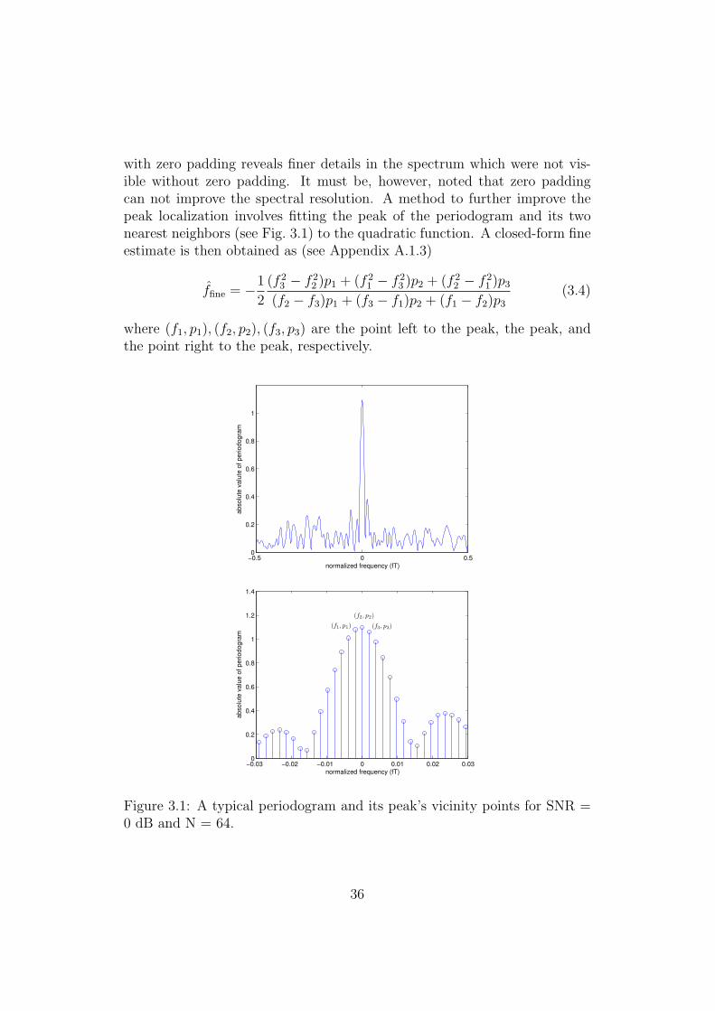
with zero padding reveals finer details in the spectrum which were not vis-ible without zero padding. It must be, however, noted that zero paddingcan not improve the spectral resolution. A method to further improve thepeak localization involves fitting the peak of the periodogram and its twonearest neighbors (see Fig. 3.1) to the quadratic function. A closed-form fineestimate is then obtained as (see Appendix A.1.3)

ffine = −1

2

(f 23 − f 2

2 )p1 + (f 21 − f 2

3 )p2 + (f 22 − f 2

1 )p3

(f2 − f3)p1 + (f3 − f1)p2 + (f1 − f2)p3

(3.4)

where (f1, p1), (f2, p2), (f3, p3) are the point left to the peak, the peak, andthe point right to the peak, respectively.

−0.5 0 0.50

0.2

0.4

0.6

0.8

1

normalized frequency (fT)

ab

so

lute

va

lute

of

pe

rio

do

gra

m

−0.03 −0.02 −0.01 0 0.01 0.02 0.030

0.2

0.4

0.6

0.8

1

1.2

1.4

normalized frequency (fT)

ab

so

lute

va

lue

of

pe

rio

do

gra

m

(f1, p1)

(f2, p2)

(f3, p3)

Figure 3.1: A typical periodogram and its peak’s vicinity points for SNR =0 dB and N = 64.

36

3.1.2 Approximated maximum likelihood estimators

The MLE is known to provide the optimal estimate of f0, however, it isprohibited from several applications because of it’s high computational re-quirement. In the past years, there are many significant contributions inapproximated MLE which yield simpler form of estimators. The approxi-mated maximum likelihood estimators presented here represent the state-of-the-art in frequency estimation. The main ideas and useful derivations foreach estimator are therefore summarized in Appendix A.

Tretter estimator

Tretter [18] proposed an approach that provides the significant insightfulresult that frequency and phase estimation can be equivalently seen as thelinear regression of the phase data. Tretter first proved that for a sufficientlyhigh SNR, the complex noise, n(k), can be transformed to the phase noise,vQ(k), with the variance reduced by factor of 2 (see Appendix A.1.5)

arg {y(k)} ≈ [2πkf0 + φ+ vQ(k)]π−π (3.5)

where y(k) is the received signal defined in (3.1) with arg{x} representingthe angle of x, vQ(k) is a real-valued zero-mean white Gaussian noise withvariance σ2

n/(2|a|2), and [x]π−π is the modulo-2π operation.He further suggested estimating f0 and φ by linear regression on the signal

phase. Tretter estimator has the form of (see Appendix A.1.6)

f0 =12

2πN(N2 − 1)

N−1∑

k=0

[k − (N − 1)

2

]arg {y(k)} . (3.6)

Note that a phase unwrapping procedure is needed for arg {y(k)}.A simple one-dimension phase unwrapping procedure based on Itoh’s

analysis [19] is summarized in the following steps. This procedure unwrapsthe phase in the array ψ(i) ∈ (−π, π] for 0 ≤ i < M − 1. In this caseψ(i) , arg{y(i)}.

• Compute phase differences: D(i) = ψ(i+1)−ψ(i) for i = 0, . . . ,M−2.

• Compute the wrapped phase differences: ∆wp(i) = arctan{ sinD(i)cosD(i)

} fori = 0, . . . ,M − 2.

• Initialize the first unwrapped value: φ(0) = ψ(0).

37

• Unwrap by summing the wrapped phase differences: φ(i) = φ(i− 1) +∆wp(i− 1) for i = 1, . . . ,M − 1.

Kay estimator

The only difficulty with Tretter estimator is that the phase needs to beunwrapped in computing f0 and φ. This phase unwrapping, besides addingto the computation, may prove to be difficult at lower SNR’s. To avoid phaseunwrapping, Kay [20] derived an estimator based on the phase differencesbetween two consecutive samples. The phase differences take the form of

∆ϕ(k) = arg {y(k)y∗(k − 1)}≈ 2πf0 + vQ(k) − vQ(k − 1)

(3.7)

provided that |2πf0| < π and vQ(k) is sufficiently small. It is clear from (3.7)that the problem now is to estimate the mean f0 of a colored Gaussian noiseThe maximum-likelihood estimate of f0 is found as (see Appendix A.1.7)

f0 =1

2π

N−1∑

k=1

6k(N − k)

N(N2 − 1)∆ϕ(k). (3.8)

The estimation variance of Kay estimator is shown to attain the CRLB athigh SNR. Kay also suggested to interchange the summation and the argu-ment operations in (3.8), however resulting in an inferior alternative to hisoriginal one. The analysis of this comment from Kay has been carried outin [21]. The generalized Kay estimator with arbitrary lag greater than one,is derived in [22].

Fitz estimator

A promising approach for single frequency estimation relying on calculatingor approximating the autocorrelation of the received signal, is known to pro-vide a good threshold. This concept was first introduced by Fitz [23] [24]and later improved by Luise and Reggiannini (L&R estimator) [25]. Fitz

38

estimator has the form of (see Appendix A.1.8)

f0 =1

2π

L∑

m=1

6m

N(N + 1)(2N + 1)arg {r(m)} . (3.9)

where r(m) is the estimated autocorrelation of the samples, y(k), defined as

r(m) =1

N −m

N−1∑

k=m

y(k)y∗(k −m), 1 ≤ m ≤ L (3.10)

where L is the design parameter not greater than N2. Note that the estimation

range of Fitz estimator is limited to |f0| ≤ 12L

. To enlarge the range, phaseunwrapping algorithm such as the one presented previously can be used. Theoptimal value of L is found to be ∼ 17N/20.

Mengali estimator

Though Fitz estimator is accurate (the estimation variance attains the CRLB)even at low SNR, it suffers from the relatively small estimation range. Men-gali and Morelli [26] derived an estimator based on the phase differences ofsample correlations which is conceptually similar to Kay’s approach. Theestimation range of the Mengali estimator is about ±50% of the symbol rateat high SNR. Mengali estimator has the form of (see Appendix A.1.9)

f0 =3

2π

L∑

m=1

(N −m)(N −m+ 1) − L(N − L)

L(4L2 − 6LN + 3N2 − 1)∆ϕ(m) (3.11)

where ∆ϕ(m) = arg {r(m)r∗(m− 1)} and r(m) is similar to (3.10). Theestimation variance of Mengali estimator attains the CRLB when L = N/2.

3.1.3 Proposed estimators

In comparing the estimators, the following four performance figures are fre-quently referred to: Accuracy : estimation error variance, Estimation range:unambiguous estimation region, Threshold : the SNR below which large es-timation errors begin to occur, and Implementation complexity : number of

39

operations.These figures are usually contradicting each other. For example, achiev-

ing a low threshold implies a high complexity. Likewise, good estimationaccuracy is often paid at the price of a narrow estimation range. So a tradeoff is called for between various options which can only be made by carefullyspecifying the actual operation conditions.

Modified Kay estimator

To reduce the threshold of Kay estimator, an estimator based on averagingnoise over samples is developed [1]. The idea is to equally divide the observa-tion vector y = [y(0), · · · , y(N − 1)]T into segments, each segment containsM samples. The samples within the same segment are added together toproduce a new sample z(k) which can be expressed as (see Fig. 3.2)

z(k) =1

M

M−1∑

m=0

y(kM +m), 0 ≤ k ≤ P − 1 (3.12)

where P = NM

, and y(k) is defined as in (3.1).

M

N

M M M M

(0)z ( 1)z P(1)z

M

( 2)z P

1

M

1

M

1

M

1

M

1

M

Figure 3.2: Producing new observation sequence by segmenting and adding.

40

Substituting (3.1) into (3.12), one obtains

z(k) =|a|M

M−1∑

m=0

exp{j[2πf0(kM +m) + φ]} + n(kM +m)

= exp{j[2πf0kM + φ]} · |a|M

M−1∑

m=0

exp{j2πf0m} +|a|M

M−1∑

m=0

n(kM +m)

= exp{j2πf0kM + φ} ·(|a|M

M−1∑

m=0

exp{j2πf0m} + v(k)

)

(3.13)

where

v(k) = − exp{j[2πf0kM + φ]}|a|M

M−1∑

m=0

n(kM +m) (3.14)

are independent zero mean couple Gaussian random variables with variance

σ2v = 1

Mσ2

n

|a|2 = (SNR)−1

M.

To simplify the derivation, f0 is assumed to be sufficiently small so thatexp{j2πf0m} ≈ 1. As a result, (3.13) becomes

z(k) = exp{j[2πf0kM + φ]}(|a| + v(k)) (3.15)

as shown in [18] for high SNRs, the complex noise v(k) can be transformedinto the phase noise

z(k) = |a| exp{j[2πf0kM + φ+ vQ(k)]} (3.16)

where vQ(k) is the imaginary part of v(k) with σ2vQ

= σ2v

2.

We define the angular frequency offset as ω∆ = 2π∆f and the instan-taneous phase of z(k) as ϕ(k) , arg{z(k)} = [ω∆k + φ + vQ(k)]π−π. Toestimate the frequency offset, as suggested in [20], the phase differences of

41

two consecutive samples are considered

∆(k) = arg{z(k)z∗(k − 1)}, 1 ≤ k ≤ P − 1

= [ϕ(k) − ϕ(k − 1)]π−π= ω∆M + vQ(k) − vQ(k − 1) − 2πm(k)

(3.17)

where m(k) is an integer representing the modulo operation. For high SNR,m(k) = 0 but for small SNR, m(k) 6= 0 which leads to an ambiguity in theestimation of ∆f . However, by adding up the samples, the noise variance in(3.17) reduces by factor of 1

Mas compared to the original approach without

adding. The reduced noise variance makes the estimation of ∆f possible inthe lower SNR regions since the chances that m(k) 6= 0 decrease.

In (3.17), ∆f and ∆(k) are related in a linear fashion and the problemis to estimate a constant, ω∆, from noisy observations, ∆(k). By perform-ing the maximum-likelihood estimation over ∆(k), the maximum-likelihoodestimator is found by minimizing the log-likelihood function

J = (∆ − ω∆M l)TC−1(∆ − ω∆M l) (3.18)

where ∆ = [∆(1),∆(2), · · · ,∆(P − 1)]T , l = [1, 1, · · · , 1]T , and C is (P −1)×(P−1) covariance matrix of ∆(k). The solution is obtained by d

dω∆J = 0

which results in

ω∆ =1

M

lTC−1∆

lTC−1l. (3.19)

The covariance matrix C is found to be

C =(SNR)−1

2M

2 −1 0 0 · · · 0−1 2 −1 0 · · · 0· · · · · · · · · · · · · · · · · ·0 0 · · · 0 −1 2

. (3.20)

The inverse of (3.20) with the (i, j) element is given by

[C−1

]ij

=2M

(SNR)−1

[min(i, j) − ij

P

], i ≥ 1, j ≤ P − 1 (3.21)

42

where min(i, j) denotes the minimum between i and j.Performing some algebra based on (3.21), a closed-form estimator can be

obtained. The explicit form of C−1 is

C−1 =2M

(SNR)−1·

1 − 1P

1 − 2P

1 − 3P

· · · 1 − 1(P−1)P

1 − 2P

2 − 4P

2 − 6P

· · · 2 − 2(P−1)P

1 − 3P

2 − 6P

3 − 9P

· · · 3 − 3(P−1)P

... · · · · · · · · · ...

1 − 1(P−1)P

2 − 2(P−1)P

3 − 3(P−1)P

· · · (P − 1) − (P−1)2

P

.

(3.22)

First, lTC−1l is calculated as follows:

lTC−1 =2M

(SNR)−1· [1s− 0, 2s− 1, 3s− 3, 4s− 6, · · · ] (3.23)

where s =∑P−1

i=1

(1 − i

P

)= (P−1)

2. The result yields

lTC−1l =2M

(SNR)−1

P−1∑

k=1

(sk − k

2(k − 1)

)

=2M

(SNR)−1

((s+

1

2

) P−1∑

k=1

k − 1

2

P−1∑

k=1

k2

)

=2M

(SNR)−1· P (P 2 − 1)

12.

(3.24)

Using (3.23), lTC−1∆ can then be calculated

lTC−1∆ =2M

(SNR)−1

P−1∑

k=1

(sk − k

2(k − 1)

)∆(k)

=2M

(SNR)−1· 1

2

P−1∑

k=1

k(P − k)∆(k).

(3.25)

43

Substituting (3.24) and (3.25) into (3.19), results in a closed-form estimator

ω∆ =1

M· lTC−1∆

lTC−1l

=1

M·P−1∑

k=1

6k(P − k)

P (P 2 − 1)∆(k).

(3.26)

The corresponding estimation variance is

var(ω∆) =1

M2· 1

lTC−1l

=1

M2· 6

P (P 2 − 1)· (SNR)−1

M

=6

N(N2 −M2)· (SNR)−1.

(3.27)

If M = 1, the estimation variance attains the CRLB and the proposed esti-mator is identical to the original Kay estimator.

Improved Fitz estimator

Fitz frequency estimator [23,24] relies on the estimated sample autocorrela-tion and is known to provide efficient estimates even at low SNR. However, itsuffers from the narrow estimation range mainly caused by the phase ambigu-ities of the estimated sample autocorrelation. Kay [20] showed that the esti-mation range of an estimator which is based only on the phase of the receivedsignal can be extended if the phase difference, arg{y(m)y∗(m − 1)}, is ex-ploited, instead of the single phase, arg{y(k)}. Mengali and Morelli [26] usedthe same concept, but with the autocorrelation estimates, arg{r(m)r∗(m −1)}, of the received signal sample rather than the received signal itself. Theweighting function for such a phase difference based estimator is derivedusing maximum likelihood estimation.

To explain the benefit of using the phase difference of the estimated cor-relation, the noiseless condition is assumed. The phase of r(m) then reads

φ(m) = arg{r(m)} = [2πf0m]π−π (3.28)

44

where [x]π−π means that x is confined within the interval (−π, π]. As m variesfrom 1 to N −1, eq. (3.28) establishes a linear relation between f0 and r(m),only when f0 lies within the interval about ± 1

2N. If f0 lies outside the interval,

eq. (3.28) becomes a highly nonlinear function and introduces ambiguities.On the other hand, the phase difference of one lag reads

∆φ(m) = arg{r(m)r∗(m− 1)} = [2πf0]π−π . (3.29)

Eq. (3.29) is independent from m which means that, as long as f0 lies within±1

2, φ(m) keeps equal to 2πf0 for 1 ≤ m ≤ N − 1. Clearly, (3.29) relates

f0 and φ(m) in a linear fashion and the problem is to estimate a constant,f0, from the noisy measurements, φ(m). It can be seen that the estimationrange is enlarged roughly by a factor of N using phase differences as theobservations.

The objective is to transform Fitz estimator (3.9) of the form

f0 =1

2π

L∑

m=1

wm arg{r(m)} (3.30)

into the the estimator of the following form

f0 =1

2π

L∑

m=1

wm arg{r(m)r∗(m− 1)}. (3.31)

The direct derivation as considered by Mengali and Morelli is promising,but it can be lengthy. Alternatively, the well known summation-by-partsformula can be used for this purpose [6, 7]. This method assumes that theweighting function wm is not a constant and w0 = 0. Consider the followingsummation-by-parts formula

L∑

m=0

∆bmam = bLaL − b−1a0 −L∑

m=1

bm−1∆am (3.32)

where ∆bm = bm − bm−1 and ∆am = am − am−1. Inspecting (3.32), and the

45

summation terms in (3.30) and (3.31) yields

L∑

m=1

wm︸︷︷︸∆bm

· arg{r(m)}︸ ︷︷ ︸am

= bL arg{r(L)} −L∑

m=1

bm−1∆φ(m)

=L∑

m=1

(bL − bm−1)︸ ︷︷ ︸wm

∆φ(m)

(3.33)

where ∆b0 = 0, b−1 = 0, ∆φ(m) = arg{r(m)r∗(m − 1)}, arg{r(N − 1)} =∑N−1m=1 ∆φ(m). Since b−1 = 0 and ∆b0 = 0, one obtains

bm =m∑

k=1

∆bk. (3.34)

Inserting (3.34) into (3.33), the new weighting function wm can be calculatedfrom wm by

wm =L∑

k=1

∆bk −m−1∑

k=1

∆bk (3.35)

where ∆bk = {wm}m=k. Therefore, given wm and r(m), one can transform(3.30) to the new estimator, having the form of (3.31):

f0 =1

2π

L∑

m=1

[L∑

k=1

wk −m−1∑

k=1

wk

]∆φ(m)

=1

2π

L∑

m=1

[L−m+1∑

k=1

wL+m−1

]

︸ ︷︷ ︸wm

∆φ(m)(3.36)

The expression (3.36) can be used to transform a given estimator with theform of (3.30) to an estimator of the form (3.31).

46

The transformed Fitz estimator with the extended estimation range is

f0 =1

2π

L∑

m=1

3N(N + 1) −m(m− 1)

N(N + 1)(2N + 1)︸ ︷︷ ︸wm

arg {r(m)r∗(m− 1)} . (3.37)

Note that by comparing wm in (3.37) with wm in (3.9) it can be noticed that

wm = wm − wm+1 (3.38)

as a result, for a given wm, one can also reversely obtain wm.

Approximated ML estimators

Two correlation-based estimators are derived in this subsection. First, theabsolute phase-based estimator is derived, then the weight transformationformula (3.36) is used to transform the weighting function of the proposedabsolute phase based into differential phase based estimator.

An approximated ML estimator may be derived from a periodogram ofthe form

J(ωo) =N−1∑

n=0

N−1∑

m=0

y(n)y∗(m)e−jωo(n−m). (3.39)

The derivative of (3.39) with respect to ωo equated to zero may be rearrangedin the following form

Im

{N−1∑

m=1

m(N −m)|r(m)|ej(ϕ(m)−ωom)

}= 0. (3.40)

By assuming that the accurate phase estimates of r(m) are available, and

47

|r(m)| is a constant, (3.40) reduces to

ωo =

∑Lm=1m(N −m)|r(m)|φ(m)∑L

m=1m2(N −m)|r(m)|

=L∑

m=1

12m(N −m)

L(L+ 1)(4LN + 2N − 3L2 − 3L)︸ ︷︷ ︸wm

φ(m)(3.41)

where L < N is a design parameter.To extend the estimation range of (3.41), eq. (3.36) is then applied to wm

in (3.41) resulting in the following transformed weighting function

wm =12∑L−m+1

k=1 (k +m− 1)(N − k −m+ 1)

L(L+ 1)(4LN + 2N − 3L2 − 3L)

= 2L(L+ 1)(3N − 2L− 1) −m(m− 1)(3N − 2m+ 1)

L(L+ 1)(4LN + 2N − 3L2 − 3L).

(3.42)

Estimation variance of correlation-based estimators

Absolute phase The absolute phase based estimator reads

ωo =L∑

m=1

wmφ(m)

≈ ωo

L∑

m=1

mwm +L∑

m=1

wmγI(m)

(3.43)

where wm is the weighting function. This class of estimators is unbiasedwhen

∑Lm=1mwm = 1 and ωo ∈ [− π

L, πL). Thus, its estimation range is

approximately ±π/L. Outside this range, (3.43) becomes highly nonlinearand awkward to handle. To transform the nonlinearity into a linear equationover the entire range an additional phase unwrapping procedure is needed,however this would be difficult at low SNR.

48

The estimation variance, var(ωo) , E {(ωo − ωo)2}, of (3.43) reads

var(ωo) =L∑

m=1

L∑

n=1

wmwnE {γI(m)γI(n)}︸ ︷︷ ︸µ(m,n)

(3.44)

where

µ(m,n) =min(m,n,N −m,N − n)

SNR(N −m)(N − n)+

δm,n

2SNR2(N − n). (3.45)

The exact expression of γI(m) and the derivation of (3.45) can be foundin Appendix A.1.10.

Differential phase The differential phase-based estimator reads

ωo =L∑

m=1

wm∆φ(m)

≈ ωo

L∑

m=1

wm +L∑

m=1

wm(γI(m) − γI(m− 1))

(3.46)

where wm is the weighting function. This class of estimators is unbiasedwhen

∑Lm=1 wm = 1 and ωo lies within [−π, π). Thus, its estimation range

is about ±π or L times larger than that of (3.43) without additional phaseunwrapping algorithm.

The estimation variance of (3.46) is

var(ωo) =L∑

m=1

L∑

n=1

wmwnE {[γI(m) − γI(m− 1)][γI(n) − γI(n− 1)]}︸ ︷︷ ︸ρ(m,n)

(3.47)

where ρ(m,n) = µ(m,n) + µ(m− 1, n− 1) − µ(m− 1, n) − µ(m,n− 1).

49

Efficiency at high SNR The statistical efficiency at high SNR is

eff , limSNR→∞

var(ωo)

CRLB≥ 1. (3.48)

Substituting (3.44) and (3.47) in (3.48) yield the efficiency measures whichdepend on L and N . The minimization of the (3.48) with respect to L seemsnot to be analytically tractable. Thus the numerical minimization is carriedout to find the optimum values of L that minimize (3.48).

As a result of the numerical minimization of (3.48) for differential phasebased estimators, the efficiencies at high SNR of Mengali and Morelli, trans-formed proposed approximated ML, and modified Fitz estimators are shownin Fig. 3.3. The corresponding optimal number of lags of these estimatorsare also identified. It is found that the optimal number of lags (Mopt) forM&M is N/2, for modified Fitz is 0.86N , and for proposed approximatedML estimator is N − 1. It shall be noted that for complexity reason, the lagvalues in the vicinity of the second optimum (local optimum) may be usedwhich will significantly reduce the implementation cost.

15 20 25 30 35 40 45 50 55 601

1.05

1.1

1.15

1.2

1.25

1.3

M

Effic

iency a

t hig

h S

NR

MM

Proposed approx ML

Modified FitzN=64, SNR = infinity

MM efficiency = 1Proposed Approx ML = 1Modified Fitz = 1.01

Mopt

=32

Mopt

=63

Mopt

=55

30 40 50 60 70 80 90 100 110 1201

1.05

1.1

1.15

1.2

1.25

1.3

M

Effic

iency a

t hig

h S

NR

MM

Proposed appox ML

Modified Fitz

Mopt

=110Mopt

=64

Mopt

=127

N=128, SNR = infnity

MM efficiency = 1Proposed approx ML = 1Modified Fitz = 1.01

Figure 3.3: Efficiencies at high SNR of M&M, transformed proposed approx-imated ML, modified Fitz estimators for N=64, and 128.

3.2 Time-Varying Envelope

The traditional methods used in analysis and development of frequency es-timators employ an additive white Gaussian noise (AWGN) model with the

50

signal. However, the additive noise model is not a sufficiently realistic rep-resentative in most of the practical applications. In practice, the receivedsignal is likely to exhibit fading behavior caused by time-varying multipathpropagation or the amplifier’s nonlinearity. This fading characteristic canbe observed in the form of random time-varying envelope (also known asthe multiplicative noise). For radar applications, a real-valued time-varyingenvelope is frequently defined [27–29]. In wireless communications, on theother hand, the complex-valued time-varying envelope is usually consideredwhich can be subdivided into two categories i.e., frequency flat fading [30–34]and frequency selective fading [35–38]. In this thesis, the only frequency flatfading case is considered. An example of such a flat fading is in global satel-lite communication systems employing low and medium earth orbit satellites.In these systems, the Doppler shift of the carrier frequency varies randomlyand should be estimated and compensated for.

A general complex sinusoid that has been corrupted by fading and addi-tive noise may be modeled as

y(k) = a(k) exp{j[2πνk + θ]} + n(k), 0 ≤ k ≤ N − 1 (3.49)

where the multiplicative noise a(k) = |a(k)| exp{jφ(k)} is, in general, definedas a complex-valued Gaussian process, circular symmetric around its meanµ exp{jϕ} with µ ≥ 0 and ϕ ∈ [−π, π). ν is the normalized frequencyoffset to be estimated. The correlation function of the multiplicative noise,ra(m) = E{a(k)a∗(k − m)}, is parameterized by a real-valued1 parametervector α = [α0, · · · , αM−1]

T . Let σ2a , ra(0). Additive noise n(k) is a zero-

mean circular complex white Gaussian process with variance σ2n. a(k) and

n(k) are mutually independent. The SNR is defined as σ2a/σ

2n.

The correlation of the multiplicative noise, ra(m), is often modelled bythe following functions (see Fig. 3.4):

• Jakes model: ra(m) = σ2aJ0(2πBDT |m|)

• Sinc model: ra(m) = σ2asinc(2πBDT |m|)

• Exponential model: ra(m) = σ2a exp{−2πBDT |m|}

• Gaussian model: ra(m) = σ2a exp{−2π(BDT )2m2/4}

1This assumption has been made implicitly by many authors to ensure a consistentfrequency estimate via the correlation-based estimation approach. Otherwise, the phaseof ra(m) has to be estimated prior to the frequency estimation.

51

where BD is the Doppler bandwidth, T is the sampling time, J0(·) is the 0-thorder Bessel function of the first kind, and BDT is the normalized Dopplerspread2. For mobile cellular communications [30,31,39,40], it is customary tofollow Jakes and Sinc models. In Doppler-radar and ionospheric communica-tions [34,41], the correlation function with Exponential and Gaussian shapesare often assumed. However, it is widely recognized that the actual spec-trum of ra(m) has little impact on the overall system performance. The soleinfluential parameter is the Doppler spread, BD. The correlation functionof the multiplicative noise reflects the variability of the channel over time.This second-order statistic generally depends on the propagation geometry,velocity of the platform, and the antenna characteristics.

0 20 40 60 80 100−0.5

0

0.5

1

correlation lag ’m’

Jakes, r a

(m)

BD

T=0.1

BD

T=0.01

BD

T=0.001

0 20 40 60 80 100

−0.2

0

0.2

0.4

0.6

0.8

1

correlation lag ’m’

Sin

c, r a

(m)

BD

T=0.1

BD

T=0.01

BD

T=0.001

0 20 40 60 80 1000

0.1

0.2

0.3

0.4

0.5

0.6

0.7

0.8

0.9

1

correlation lag ’m’

Expnential, r

a(m

)

BD

T=0.1

BD

T=0.01

BD

T=0.001

0 20 40 60 80 1000

0.1

0.2

0.3

0.4

0.5

0.6

0.7

0.8

0.9

1

correlation lag ’m’

Gaussia

n, r a

(m)

BD

T=0.1

BD

T= 0.01

BD

T=0.001

Figure 3.4: Four correlation models of the multiplicative noise with slow(BDT = 0.001), intermediate (BDT = 0.01), and fast fading (BDT = 0.1).

As (3.49) represents a general signal model for CFO estimation problemin single-carrier systems, three special cases can be categorized as follows:

2Typical values for practical systems [33] range from BDT = 0.001 (very slow fading)to BDT = 0.1 (very fast fading).

52

Rayleigh fading: the amplitude of the fading process will have a Rayleighdistribution if µ = 0 and σ2

a 6= 0.

Rician fading: the amplitude of the fading process will have a Rician (dom-inant+Rayleigh) distribution if µ 6= 0 and σ2

a 6= 0.

Non-fading: or the classical constant-amplitude with only additive Gaus-sian noise (discussed in the previous section) is obtained when µ 6= 0and σ2

a = 0.

The theoretical Cramer-Rao lower bound (CRLB) is derived in the AppendixA.2.1 and is given as the corresponding diagonal element of the inverse ofthe Fisher information matrix (FIM), J−1

ωo,ωo. The CRLB is then

CRLB(ωo) = J−1ωo,ωo

(3.50)

where ωo = 2πν. The Jωo,ωois found to be

Jωo,ωo= 2µ21TDR−1D1 + 2tr{R−1DRD − D2} (3.51)

where tr is the matrix trace, R = Ra + σ2nI, 1 is a (N × 1) vector of one,

Ra(i, j) = ra(|i− j|) with i, j = 1, · · · , N , and D = diag{0, · · · , N − 1}. Forthe correlated Rayleigh channel µ = 0, and Jωo,ωo

= 2tr{R−1DRD − D2}.For high SNR or σ2

n → 0,

Jσ2n→0

ωo,ωo= 2tr{R−1

a DRaD − D2} (3.52)

is a constant which leads to the so called error floor effect.

3.2.1 Proposed estimator for complex-valued envelope

The CFO estimators proposed in the past [30–32,34] are associated with oneor more of the following limitations/drawbacks: 1). Require a priori knowl-edge on the form of the fading correlation [30, 31], 2). High computationalcomplexity [32], and 3). Short estimation range [34].

Kuo and Fitz [30] proposed to estimate the normalized (angular) fre-quency as

ωo = αT θ (3.53)

53

where θ = [θ(1), . . . , θ(M)]T , and θ(m) = m−1 arg{r(m)}, r(m) is the m-thlag correlation estimate defined in (3.56). The optimal weight vector, α, ischosen to minimize the variance of (3.53) and is given by

α =C−1θ (BDT, SNR)1

1TC−1θ (BDT, SNR)1

(3.54)

where Cθ(BDT, SNR) = E{(θ − θ)(θ − θ)T}, and 1 = [1, . . . , 1]T . It shallbe noted that Cθ(BDT, SNR) depends on BDT and SNR. This covariancematrix of phase estimation errors is assumed to be known in the work ofKuo and Fitz in [30] which is seldom available in practical situations. More-over, phase unwrapping is required which may be delicate in small samplesor in low SNR environments. To circumvent these problems, [31] proposeda similar scheme based on the difference between the phases of the correla-tion, arg{r(m)r∗(m − 1)}. Additionally, the covariance matrix of the phaseestimation errors was estimated in [31] prior to performing weighted linearregression. However, this covariance matrix estimate strongly relies on anassumed form for the correlation of the fading process. Therefore methodsin [30, 31] are sensitive to mismodeling of the fading correlation. A low-complexity CFO estimator, which does not assume nor estimate the channelparameter, was proposed in [34]. Its estimation range is, however, limited.The nonlinear least-squares estimator proposed in [32], is robust to the lack ofinformation on the form of the correlation of the fading process and is able tooperate at the maximum estimation range but at the price of computationalcomplexity.

The complexity of the estimator proposed in [32] can be reduced, butat the cost of a decreased estimation range [3]. However, It will be shownin the following sections that by using the summation-by-parts formula thecomputational complexity can be reduced without shortening the estimationrange.

Observation model

The true correlation sequence corresponding to the data model (3.49) is

r(m) = E{y(k)y∗(k −m)}= ra(m)ej2πmν + σ2

nδ(m).(3.55)

54

The estimated correlation sequence can be calculated by two standard ways,the first is

r1(m) =1

N −m

N−1∑

k=m

y(k)y∗(k −m), m = 0, 1, . . . ,M − 1 (3.56)

and the second is

r2(m) =1

N

N−1∑

k=m

y(k)y∗(k −m) (3.57)

where the former is known as the unbiased estimate of r(m) since E{r1(m)} =r(m), and the latter is known as the biased estimate of r(m), since E{r2(m)} =(1 − |m|/N) · r(m). The statistical properties of these two approaches aregiven in Appendix A.2.2.

Correlation-based nonlinear least-squares estimator

The NLS estimates of σ2n, d(m) , ra(m), and ν are obtained by solving the

following minimization problem

{σ2n, d, ν} = arg min

σ2n,d,ν

1

M

M∑

m=0

|r(m) − d(m)ej2πmν − σ2nδ(m)|2

︸ ︷︷ ︸J(σ2

n,ν,d)

. (3.58)

where r(m) can be chosen from either (3.56) or (3.57), d(m) , ra(m), andd = [d(0), · · · , d(M)]T . Setting the derivative of the criterion J(σ2

n, ν,d)w.r.t. σ2

n to zero, we obtain

σ2n = r(0) − d(0). (3.59)

Substitute this solution into J(σ2n, ν,d), yields the reduced criterion

{d, ν} = arg mind, ν

1

M

M∑

m=1

|r(m) − d(m)ej2πmν |2

︸ ︷︷ ︸J(ν,d)

. (3.60)

55

Since (3.56) is a consistent estimate of (3.55), it follows that J∞(ν,d) ,

limN→∞ J(ν,d) achieves a global minimum at the true parameters [32, 34].Consequently, ν is a consistent estimate of ν whatever form of d(m). It willbe shown that the criterion in (3.60) can be concentrated w.r.t. d so as toleave one-dimensional search over ν only. Using the fact that d(m) ∈ R,J(ν,d) can be rewritten as

M∑

m=1

{|r(m)|2 − 2d(m)Re

{r(m)e−j2πmν

}+ d2(m)

}. (3.61)

Taking the derivative of (3.61) w.r.t. d and equating the result to zero, yields

d(m) = Re{r(m)e−j2πmν

}(3.62)

where the estimate of the frequency offset has yet to be determined. Inserting(3.62) into (3.61), the NLS estimate of the parameter ν is obtained as

νNLS = arg maxν

Re

{M∑

m=1

r2(m)e−j4πmν

}(3.63)

which can be efficiently realized by means of Fast Fourier Transform (FFT)with zero padding. This can be done by O(Nf log2Nf ) operations, whereNf is the Fourier bins. A better localization of the peak can be obtained byusing the quadratic interpolation as introduced in (3.4).

However, a much simpler form of (3.63) is obtained by assuming theavailability of the phase of the correlation estimate, φm = arg{r(m)}. TheNLS criterion (3.63) can be rewritten as

M∑

m=1

|r(m)|2 cos(2φm − 4πmν). (3.64)

Setting the derivative of (3.64) w.r.t. ν to zero, we obtain

M∑

m=1

m|r(m)|2 sin(2φm − 4πmν) = 0. (3.65)

56

Under the small error approximation, i.e., sin(2φm−4πmν) ≃ (2φm−4πmν),the simplified NLS (SNLS) estimator is obtained as

νSNLS =1

2π

∑Mm=1m|r(m)|2φm∑Mm=1m

2|r(m)|2

=M∑

m=1

αmφm

(3.66)

where αm is the weighting function of the absolute phase-based estimator.Note that without an additional phase unwrapping algorithm, e.g., [19],

the estimation range of the SNLS is limited to about ±1/2M the symbolrate.

Weight transformation formula

Using Am =∑m

k=0 αk, φM =∑M

m=1(φm − φm−1), and A−1 = 0, the relation-ship between the absolute phase based and phase difference based estimatorsis derived as

M∑

m=0

αmφm =M∑

m=0

(Am − Am−1)φm

=M∑

m=0

Amφm −M−1∑

m=−1

Amφm+1

=AMφM − A−1φ−1 +M−1∑

m=0

Am(φm − φm+1)

=AMφM −M∑

m=1

Am−1(φm − φm−1)

=M∑

m=1

(AM − Am−1)(φm − φm−1)

=M∑

m=1

(M∑

k=1

αk −m−1∑

k=1

αk

)

︸ ︷︷ ︸βm

∆φm.

(3.67)

57

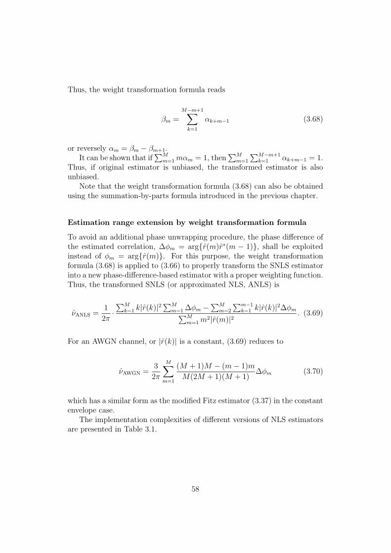
Thus, the weight transformation formula reads

βm =M−m+1∑

k=1

αk+m−1 (3.68)

or reversely αm = βm − βm+1.It can be shown that if

∑Mm=1mαm = 1, then

∑Mm=1

∑M−m+1k=1 αk+m−1 = 1.

Thus, if original estimator is unbiased, the transformed estimator is alsounbiased.

Note that the weight transformation formula (3.68) can also be obtainedusing the summation-by-parts formula introduced in the previous chapter.

Estimation range extension by weight transformation formula

To avoid an additional phase unwrapping procedure, the phase difference ofthe estimated correlation, ∆φm = arg{r(m)r∗(m − 1)}, shall be exploitedinstead of φm = arg{r(m)}. For this purpose, the weight transformationformula (3.68) is applied to (3.66) to properly transform the SNLS estimatorinto a new phase-difference-based estimator with a proper weighting function.Thus, the transformed SNLS (or approximated NLS, ANLS) is

νANLS =1

2π·∑M

k=1 k|r(k)|2∑M

m=1 ∆φm −∑Mm=2

∑m−1k=1 k|r(k)|2∆φm∑M

m=1m2|r(m)|2

. (3.69)

For an AWGN channel, or |r(k)| is a constant, (3.69) reduces to

νAWGN =3

2π

M∑

m=1

(M + 1)M − (m− 1)m

M(2M + 1)(M + 1)∆φm (3.70)

which has a similar form as the modified Fitz estimator (3.37) in the constantenvelope case.

The implementation complexities of different versions of NLS estimatorsare presented in Table 3.1.

58

Estimators Number of complex multiplications

FFT-based NLS Nf log2Nf + M(2N−M−1)2

SNLS M(2N−M−1)2

+ Phase unwrapping

ANLS M(2N−M−1)2

+ (M − 2)

AWGN M(2N−M−1)2

+ (M − 2)

Table 3.1: Complexity of different versions of NLS estimators.

3.2.2 Proposed EKF for real-valued envelope

As a special case of the complex-valued envelope, the real-valued envelope isalso frequently used in radar applications, e.g., [27–29]. The signal envelope,a(t), is real-valued and can be modelled as random (multiplicative noise) ordeterministic but time varying. If the batch processing is considered, goodexamples can be found in [27, 42]. This model has been applied to a realapplication in estimating particle’s velocity in the vicinity of an aircraft bymeans of a laser velocimeter [43, 44]. In the following, a recursive frequencytracker known as Kalman filter, is proposed. The signal envelope is assumedto be real-valued and deterministic. Since the frequency to be estimatedis governed by the nonlinear complex exponential function, therefore theextended Kalman filter (EKF) shall be formulated [4, 45].

Extended Kalman filter

In this subsection, the system state and observation models are formulated.The Kalman filtering algorithm is given. The stochastic observability andthe alternative of the Kalman filter are briefly discussed.

System state model

The continuous system state is defined by

x(t) = [a(t) a(t) ψ(t) ψ(t)]T (3.71)

where ψ(t) is the instantaneous phase of y(k) with ψ(t) as its derivative. a(t)is the derivative of a(t).

The discrete system state is obtained by letting xk = x(t)|t=kT

xk = [x1,a(k) x2,a(k) x1,p(k) x2,p(k)]T . (3.72)

59

The difference equations of the time-varying amplitude are defined as

x1,a(k + 1) = x1,a(k) + x2,a(k)

x2,a(k + 1) = x2,a(k) + wa(k).(3.73)

The time-varying instantaneous phase can also be modelled in the same way

x1,p(k + 1) = x1,p(k) + 2π · x2,p(k)

x2,p(k + 1) = x2,p(k) + wp(k).(3.74)

The corresponding discrete time state-space model can then be expressed as

xk+1 =

1 1 0 00 1 0 00 0 1 2π0 0 0 1

· xk +

0wa(k)

0wp(k)

= A · xk + wk

(3.75)

where A is the state transition matrix, E{wk} = 0 and E{wkwTj } = Q(k) ·

δ(k, j).

Observation model

We define the first two elements of the observation vector from the inphaseand quadrature component of (3.49)

yI(k) = a(k) cos (2πνk + θ) + vI(k)

yQ(k) = a(k) sin (2πνk + θ) + vQ(k).(3.76)

We introduce a further observation, yp(k) = arg{r(k)}, which can be approx-imated at high SNR [18] as

yp(k) ≈ 2πνk + ϕk + vp(k)|mod2π (3.77)

vI(k), vQ(k) and vp(k) are regarded as the components of a vectorial zeromean white Gaussian measurement noise vector vk with diagonal covariance

60

matrix R(k) = E{vkvTk } = σ2diag{1, 1, 1E{a2(k)}}. Summarizing we have a

vectorial nonlinear observation model

yk = h(xk) + vk

yI(k)yQ(k)yp(k)

=

a(k) cos(ψ(k))a(k) sin(ψ(k))

ψ(k)

+

vI(k)vQ(k)vp(k)

(3.78)

where ψ(k) = 2πνk+ θ, xk is the state vector, h(·) is the nonlinear mappingbetween yk and xk.

Note that on the first sight yp(k) appears redundant, as one might arguethat any deterministic combination of the existing measurements does notprovide any new (innovating) information. This would be true if we weredealing with linear models but for this nonlinear case, the linearizations ig-nore the information that would be present if higher order approximationsof the nonlinear observation model were used. Hence the additional formula-tion of a nonlinear relationship will provide a different aspect of informationcontained in the other observations and thus make the filter operation morestable. Therefore, we can expect to improve the observability by introducingsuch an additional observation [46].

Kalman filtering algorithm

Once having found the state and observation model, the Kalman filter isreadily formulated [46, 47]. The specific points of interest arise from thegiven nonlinear observation model. A simple but effective solution is theextended linearized Kalman filter which linearizes the nonlinear observationmapping around the prediction estimate, x−

k . The filtering algorithm is

• Initialization

x+0 = E{x0} = x0

P+(0) = E{(x0 − x0)(x0 − x0)T} = P(0)

• Prediction

x−k+1 = Ax+

k+1

P−(k + 1) = AP+(k)AT + Q

61

• Correction

K(k + 1) = P−(k + 1)HT (k + 1)

·[H(k + 1)P−(k + 1)HT (k + 1) + R]−1

resk+1 = yk+1 − h(x−k+1)

Do while |resk+1| > π :

{res3,k+1 = res3,k+1 − sing(res3,k+1) · 2π}x+k+1 = x−

k+1 + K(k + 1) · resk+1

P+(k + 1) = [I − K(k + 1)H(k + 1)]P−(k + 1)

The linearized observation matrix (Jacobian matrix) is given by

H(k) =∂

∂xkh(xk)|xk=x

−

k=

∂yI(k)∂x1,a

∂yI(k)∂x2,a

∂yI(k)∂x1,p

∂yI(k)∂x2,p

∂yQ(k)

∂x1,a

∂yQ(k)

∂x2,a

∂yQ(k)

∂x1,p

∂yQ(k)

∂x2,p

∂yp(k)

∂x1,a

∂yp(k)

∂x2,a

∂yp(k)

∂x1,p

∂yp(k)

∂x2,p

xk=x−

k

.(3.79)

Stochastic observability

It is useful to consider stochastic observability of the modeling since it isclosely related to the stability of the filter. Stochastic observability can beproven by considering Fisher’s Information [47] defined as

F(k, k − L+ 1) =k∑

i=k−L+1

AT (i, k)HT (i)R−1H(i)A(i, k). (3.80)

The parameter is said to be stochastically observable if the diagonal elementof (3.80) increases monotonically. It is numerically shown in Fig. 3.5 thatthe EKF in which the instantaneous phase is incorporated as an additionalmeasurement, acquires more information than the one without incorporating.

62

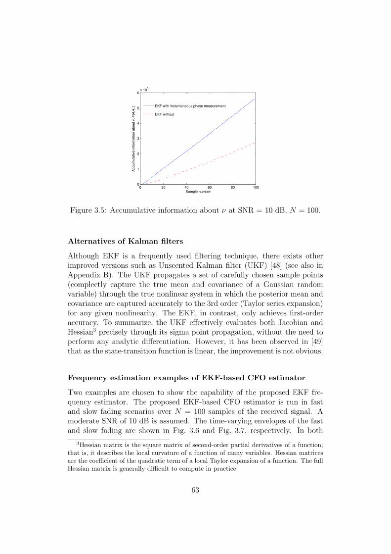
0 20 40 60 80 1000

1

2

3

4

5

6x 10

5

Sample number

Accu

mu

lative

in

form

atio

n a

bo

ut

ν,

F(4

,4,:

) EKF with instantaneous phase measurement

EKF without

Figure 3.5: Accumulative information about ν at SNR = 10 dB, N = 100.

Alternatives of Kalman filters

Although EKF is a frequently used filtering technique, there exists otherimproved versions such as Unscented Kalman filter (UKF) [48] (see also inAppendix B). The UKF propagates a set of carefully chosen sample points(complectly capture the true mean and covariance of a Gaussian randomvariable) through the true nonlinear system in which the posterior mean andcovariance are captured accurately to the 3rd order (Taylor series expansion)for any given nonlinearity. The EKF, in contrast, only achieves first-orderaccuracy. To summarize, the UKF effectively evaluates both Jacobian andHessian3 precisely through its sigma point propagation, without the need toperform any analytic differentiation. However, it has been observed in [49]that as the state-transition function is linear, the improvement is not obvious.

Frequency estimation examples of EKF-based CFO estimator

Two examples are chosen to show the capability of the proposed EKF fre-quency estimator. The proposed EKF-based CFO estimator is run in fastand slow fading scenarios over N = 100 samples of the received signal. Amoderate SNR of 10 dB is assumed. The time-varying envelopes of the fastand slow fading are shown in Fig. 3.6 and Fig. 3.7, respectively. In both

3Hessian matrix is the square matrix of second-order partial derivatives of a function;that is, it describes the local curvature of a function of many variables. Hessian matricesare the coefficient of the quadratic term of a local Taylor expansion of a function. The fullHessian matrix is generally difficult to compute in practice.

63

cases, the phase can be successfully unwrapped via EKF algorithm. Thecorresponding frequency estimates in fast and slow fading are also presentedin Fig. 3.6 and Fig. 3.7. However, the main attraction of EKF-based estima-tor is that it can be easily extended to track time-varying frequencies whichwould be relatively difficult in the case of batch processing.

10 20 30 40 50 60 70 80 90 1000

0.1

0.2

0.3

0.4

0.5

0.6

0.7

0.8

0.9

1

Iteration number, (k)

fast

fad

ing

, a

(k)

10 20 30 40 50 60 70 80 90 100−10

0

10

20

30

40

50

60

70

Iteration number, (k)

Ph

ase

, (r

ad

)

Actual phase

EKF Unwrapped phase

Wrapped phase

fast fadingSNR = 10 dB

10 20 30 40 50 60 70 80 90 1000.05

0.1

0.15

0.2

0.25

0.3

Iteration number (sample)

Fre

qu

en

cy e

stim

ate

s

Actual frequency

Estimated frequency

fast time−varying amplitude,SNR = 10 dB

10 20 30 40 50 60 70 80 90 10010

−7

10−6

10−5

10−4

10−3

10−2

10−1

100

Iteration number (sample)

Ab

so

lute

va

lue

s o

f d

iffe

ren

ce

s b

etw

ee

n a

ctu

al a

nd

estim

ate

d

fast time−varying amplitude,SNR = 10 dB

Figure 3.6: Frequency estimates in fast fading real-valued amplitude.

3.3 Simulation Results

3.3.1 Non-fading channel

In the non-fading channels, the estimation ranges and the mean-squares er-ror (MSE) of the ML, Kay, Modified Kay, Fitz, Modified Fitz, proposedapproximated ML, and Mengali estimators are shown. The advantages anddisadvantages of these estimators can be seen from the simulation results

64

10 20 30 40 50 60 70 80 90 1000.955

0.96

0.965

0.97

0.975

0.98

0.985

0.99

0.995

1

Iteration number, (k)

fast

fad

ing

, a

(k)

0 20 40 60 80 100−10

0

10

20

30

40

50

60

70

Iteration number, (k)

Ph

ase

, (r

ad

)

Actual phase

EKF Unwrapped phase

Wrapped phase

slow fadingSNR = 10 dB

10 20 30 40 50 60 70 80 90 1000.08

0.1

0.12

0.14

0.16

0.18

0.2

Iteration number (sample)

Fre

qu

en

cy e

stim

ate

s

Actual frequency

Estimated frequency

Slow time−varying amplitude,SNR = 10 dB

10 20 30 40 50 60 70 80 90 10010

−7

10−6

10−5

10−4

10−3

10−2

10−1

100

Iteration number (sample)

Ab

so

lute

va

lue

s o

f d

iffe

ren

ce

s b

etw

ee

n a

ctu

al a

nd

estim

ate

d

Slow time−varying amplitude,SNR = 10 dB

Figure 3.7: Frequency estimates in slow fading real-valued amplitude.

presented in Fig. 3.8 and Fig. 3.9. The data model of (3.1) with N = 128 isused in all simulations.

Although the ML estimator is attractive as it attains the CRLB even ata very low SNR and has the maximum estimation range of ±0.5 the symbolrate, it’s complexity is prohibitive. This can be observed in Fig. 3.9 that therequired number of Fourier bin (Nf ) followed by the interpolation isNf = 512for ML estimator to attain the CRLB. Without at additional interpolationmethod, the ML estimator requires at least Nf = 220 = 1048576.

Kay estimator is much simpler than the ML estimator and has also themaximum estimation range of about ±0.5 the symbol rate but its threshold ismuch higher than that of the ML estimator. This problem has been reducedby the modified Kay estimator in which the threshold can be improved as thelength of the segment is increased. The accuracy of the modified Kay esti-mator reduces, but insignificantly. Moreover, the complexity of the modifiedKay estimator reduces as the size of the segment increases.

Fitz estimator (with the optimal lag of N/2) attains the CRLB even atSNR as low as zero dB. However, it’s estimation range with the optimal lag

65

−0.4 −0.2 0 0.2 0.4 0.6

−0.4

−0.2

0

0.2

0.4

0.6

Normalized frequency offset (fT)

Mean o

f th

e fre

quency e

stim

ate

s

SNR = 20 dB

SNR = 15 dB

SNR = 10 dB

Ideal

ML estimator

−0.4 −0.2 0 0.2 0.4 0.6

−0.4

−0.2

0

0.2

0.4

0.6

Normalized frequency offset (fT)

Mean o

f th

e fre

quency e

stim

ate

s

SRN = 20 dB

SNR = 15 dB

SNR = 10 dB

Ideal

Kay estimator

−0.4 −0.2 0 0.2 0.4 0.6

−0.4

−0.2

0

0.2

0.4

0.6

Normalized frequency offset (fT)

Mean o

f th

e fre

quency e

stim

ate

s

M = 1 (Kay)

M = 2

M = 4

M = 8

Ideal

Modified Kay estimator

−0.4 −0.2 0 0.2 0.4 0.6

−0.4

−0.2

0

0.2

0.4

0.6

Normalized frequency offset (fT)

Mean o

f th

e fre

quency e

stim

ate

s

L = 8

L = 4

L = 2

Ideal

Fitz estimator

−0.4 −0.2 0 0.2 0.4 0.6

−0.4

−0.2

0

0.2

0.4

0.6

Normalized frequency offset (fT)

Mean o

f th

e fre

quency e

stim

ate

s

L = 8

L = 4

L = 2

Ideal

Modified Fitz estimator

−0.4 −0.2 0 0.2 0.4 0.6

−0.4

−0.2

0

0.2

0.4

0.6

Normalized frequency offset (fT)

Mean o

f th

e fre

quency e

stim

ate

s

L = 8

L = 4

L = 2

Ideal

Mengali estimator

Figure 3.8: Estimation ranges of different CFO estimators for single carriersignal with constant amplitude, with N = 128, SNR = 20 dB.

(L = N/2) is very small and limited to about 1/2L = 1/N . To solve the phaseambiguity problem directly, an additional phase unwrapping algorithm [19]is required.

With the use of the summation-by-parts formula, the modified Fitz es-timator is able to maintain a similar accuracy as Fitz estimator, but theestimation range is extended to about ±0.5 the symbol rate. The accuracy

66

0 5 10 15 2010

−9

10−8

10−7

10−6

10−5

SNR (dB)

MS

E

CRLB

Nf=2

9 + interp

Nf=2

12 without interp

Nf=2

13 without interp

Nf=2

20 without interp

ML estimator

f0 = 0.0

−5 0 5 10 15 2010

−10

10−9

10−8

10−7

10−6

10−5

10−4

10−3

SNR (dB)

MS

E

M = 1 (Kay)

M = 2

M = 4

M = 8

CRLB

Kay and Modified Kay estimators

f0 = 0.0

−5 0 5 10 15 2010

−10

10−9

10−8

10−7

10−6

10−5

10−4

10−3

SNR (dB)

MS

E

L = 4

L = 8

L = 16

L = 32

L = 64

CRLB

f0 = 0.0

Fitz estimator

−5 0 5 10 15 2010

−10

10−9

10−8

10−7

10−6

10−5

SNR (dB)

MS

E

CRLB

Fitz, Lopt

= N/2 = 64

Modified Fitz, Lopt

= N/2 = 64

Fitz and Modified Fitz estimators

f0 = 0.0

−5 0 5 10 15 2010

−10

10−9

10−8

10−7

10−6

10−5

10−4

10−3

SNR (dB)

MS

E

L = 4

L = 8

L = 16

L = 32

L = 64

CRLB

Mengali estimator

f0 = 0.0

−5 0 5 10 15 2010

−10

10−9

10−8

10−7

10−6

10−5

SNR (dB)

MS

E

CRLB

Modified Fitz, Lopt

= 64

Mengali, Lopt

= 64

Modified Fitz vs. Mengali estimators

f0 = 0.0

Figure 3.9: MSE versus SNR of different CFO estimators for single carriersignal with constant amplitude, with N = 128, f0 = 0.0.

and the estimation range of the modified Fitz are comparable to the Men-gali estimator, however the derivation of the modified Fitz is somewhat lesscomplicated than the Mengali estimator.

Fig. 3.10 (left) compares the ratio between the estimation variance andthe CRLB of Mengali, modified Fitz, transformed proposed estimators versusSNR, with N = 64, M = Mopt, and ωo = 0.1 × 2π. It can be seen that the

67

efficiency of Mengali is better than that of the modified Fitz at high SNRbut worse in lower SNR regions. The transformed proposed approximatedML estimator performs better than Mengali, and modified Fitz estimatorsespecially at moderate/low SNRs.

Fig. 3.10 (right) compares the MSEs of the transformed proposed approx-imated ML and Mengali estimators versus SNRs with N = 64, M = 4, 8, 16,and ωo = 0.1 × 2π. This is to show the performances when the complexityis more important and the accuracy can be relaxed. In all cases, the trans-formed proposed approximated ML performs better than Mengali estimatorat moderate/low SNRs.

2 4 6 8 10 12 14 16 18 200.99

1

1.01

1.02

1.03

1.04

1.05

1.06

1.07

1.08

SNR(dB)

Var(ω

o)

CRLB

Transformed proposed

Mengali & Morelli

Modified Fitz

ideal

N = 64, M = Mopt , ωo = 0.1 × 2π

0 5 10 15 2010

−9

10−8

10−7

10−6

10−5

10−4

SNR (dB)

MSE

CRLB

M&M (M=4)

trans. proposed (M=4)

M&M (M=8)

trans. proposed (M=8)

M&M (M=16)

trans. proposed (M=16)

N = 64, ωo = 0.1 × 2π

Figure 3.10: Performance comparisons of Mengali, transformed proposedapproximated ML, modified Fitz estimators.

3.3.2 Fading channel

For simulation purposes, a reliable and widely accepted autoregressive-basedmethod proposed in [40] is used to generate the realizations of the complex-valued multiplicative noise, a(k), for any arbitrarily given autocorrelationmodel, ra(m), (e.g., Jakes, Sinc, Exponential, or Gaussian models).

The data sequence of length N = 128 were generated according to (3.49)with the correlation of the multiplicative noise that obeys an exponential-shaped correlation, i.e., ra(m) = σ2

a exp{−2π|m|BDT}. The performance ofthe proposed estimator is compared to an efficient estimator proposed in [50][41] which is known as the Single-Lag (SL) estimator and given as νSL =arg{r(mopt)}/mopt, for mopt 6= 1 the ambiguities of the frequency estimatesare introduced and if not resolved the estimation range is limited to about±1/2mopt. We also compare our proposed ANLS estimator with the well

68

known CFO estimator introduced by Mengali and Morelli [26] (MMAWGN)which was originally designed to be optimum for the AWGN channel. Themean-square-error (MSE) is obtained by 20000 Monte Carlo trials. In allsimulations, the performances between ANLS and SNLS are similar, but theestimation range of SNLS is limited to ±1/2M the symbol rate while ANLScan operate at the maximum possible range of about ±0.5 the symbol rate.

Fig. 3.11 shows that in the non-fading channels the performances of theproposed ANLS and MMAWGN estimators using M = 127 attain the CRLBeven at SNR as low as zero dB, while the SL estimator, with the optimal lagof mopt = 2N/3 (see [50] [41]) is only close to the CRLB. Moreover with the

0 5 10 15 2010

−10

10−9

10−8

10−7

10−6

SNR (dB)

MS

E

SNLS

SL

ANLS

MMAWGN

CRLB

ν = 0, BDT = 0

M = 64, mopt = 85

Figure 3.11: MSE versus SNR of the ANLS, MMAWGN, SNLS and SL es-timators for ν = 0, BDT = 0 (non-fading channel) with the optimal lagvalues.

optimal lag, the estimation range of SL estimator is limited to only about±1/2M the symbol rate as can be seen in Fig. 3.12. On the other hand, theestimation ranges of ANLS and MMAWGN are shown to be independent ofthe lag number and covers about ±0.5 the symbol rate.

Fig. 3.13 compares the proposed ANLS and MMAWGN estimators in aslow fading channel (BDT = 0.0001). The lag values (M) are set to 16 and32 for both estimators. For both lag values, the proposed ANLS estimatorperforms better than the MMAWGN estimator, especially in the low SNRregion. However, their performances in the AWGN channel are similar ascan be seen in Fig. 3.11.

69

−0.5 0 0.5

−0.4

−0.2

0

0.2

0.4

0.6

Normalized frequency offset

avera

ge fre

quency e

stim

ate

s

−0.02 −0.01 0 0.01 0.02−0.02

−0.015

−0.01

−0.005

0

0.005

0.01

0.015

0.02

Normalized frequency offset

CRLB

SNLS

SL

CRLB

ANLS,MM

AWGN

BDT = 0 BDT = 0

Figure 3.12: Estimation range of the ANLS, MMAWGN, SL, and SNLS esti-mators for BDT = 0 (non-fading), with SNR = 10 dB.

−5 0 5 10 15 2010

−7

10−6

10−5

10−4

SNR (dB)

MS

E

ANLS, M=16

MMAWGN

, M=16

ANLS, M=32

MMAWGN

, M=32

CRLB

CRLB

ν = 0, BDT = 0.0001

M = 32

M = 16

Figure 3.13: MSE versus SNR of the ANLS and MMAWGN estimators forν = 0, BDT = 0.0001 (slow fading channel) for lag values of M = 16 and 32.

Fig. 3.14 shows the optimal choice of the correlation lag for the SL, SNLS,

70

and ANLS estimators in fast and moderate fading. In moderate fading, thesame optimal lag of 5 is observed for SL, SNLS, and ANLS. In fast fading,the optimal lag for SL is 2 and for SNLS and ANLS is 3. It is seen thatthe proposed ANLS estimator is less sensitive to the wrong choice of the lagnumbers than the SL estimator.

2 4 6 8

10−4.7

10−4.6

correlation lag

MS

E

2 4 6 8

10−5.58

10−5.55

10−5.52

10−5.49

10−5.46

10−5.43

correlation lag

SL

SNLS

ANLS

SL

SNLS

ANLS

BDT = 0.01 BDT = 0.001

Figure 3.14: MSE versus correlation lag in fast (BDT = 0.01) and moderatefading (BDT = 0.001), with SNR = 10 dB, ν = 0.01, N = 128.

Fig. 3.15 shows the estimation ranges of the SL, SNLS, ANLS estimatorsin moderate fading, however, we observed the same results also in fast fading.It is confirmed again that the estimation range of the proposed ANLS isindependent of number of lag and covers the maximum possible range ofabout 50% the symbol rate, which is not achievable for SL, and SNLS withoutapplying the additional phase unwrapping procedure.

Fig. 3.16 shows the performances of the SL, SNLS, and ANLS estimatorsin moderate and fast fading. The performances of ANLS and SNLS areslightly better than that of the SL for both scenarios. All attain the CRLBat high SNR. It can be observed that the estimation variance does not vanishas σ2

n → 0. This behavior is known as the error floor effect which can beexplained by (3.52). As the exponential model for the autocorrelation of themultiplicative noise is adopted, the closed-form expression of CRLB at high

71

−0.4 −0.2 0 0.2 0.4 0.6

−0.4

−0.2

0

0.2

0.4

0.6

Normalized frequency offset

Avera

ged fre

quency e

stim

ate

s

Ideal

SNLS

SL

ANLS

BDT = 0.001

Figure 3.15: Estimation ranges of SL, SNLS, ANLS estimators for BDT =0.001 with M = 5, SNR = 10 dB, N = 128.

SNR [34] can be expressed as

CRLB(ωo)σ2n→0 =

1 − exp{−2πBDT}2(N − 1) exp{−4πBDT}

. (3.81)

Thus the potential accuracy of frequency estimation decreases with increasingDoppler spread.

3.4 Summary

For constant amplitude case, the modified Kay estimator is shown to be sim-pler and more robust than the original Kay estimator. The modified Fitzestimator uses the well known summation-by-parts formula (weight transfor-mation formula) to overcome the phase ambiguity problem in Fitz estimator.At low SNRs, the performance of the modified Fitz estimator is slightly bet-ter than that of the Mengali estimator but worse at higher SNR regions.However, the modified Fitz estimator was derived with somewhat less effortthan Mengali estimator. The proposed approximated ML estimator is trans-

72

−5 0 5 10 15 2010

−6

10−5

10−4

10−3

SNR (dB)

MS

E

ANLS, BD

T=0.01, M=3

SL, BD

T=0.01, mopt

=2

ANLS, BD

T=0.001, M=5

SL, BD

T=0.001, mopt

=5

CRLB

CRLB

ν = 0.005

Figure 3.16: MSE versus SNR of ANLS and SL estimators for BDT = 0.01and BDT = 0.001 with the optimal lag values.

formed using the weight transformation formula to obtain its phase differenceversion. The performance of the transformed proposed approximated ML es-timator with optimal lag is better than that of Mengali estimator. Evenusing the same lags for low complexity, the transformed proposed approxi-mated ML estimator exhibits better performance at intermediate/low SNRs.

For time-varying amplitude especially in the case of complex multiplica-tive noise, a new closed-form correlation-based frequency estimator for signalswith fading-induced multiplicative noise is presented. It is shown that theproposed estimator can operate at the maximum estimation range of about±0.5 the symbol rate without sacrificing its accuracy and does not rely onany assumed form of the fading correlation as needed for most of the existingestimators. The features of the proposed ANLS estimator, as compared tothe previously proposed estimators, are summarized in Table 3.2.

For real-valued time-varying amplitude, the extended Kalman filter-basedrecursive CFO estimator is proposed which can be easily extended for fre-quency tracking problems.

73

Estimator Corr. form Doppler spread Unwrapping Complexity

K&F [30] required assumed required highM&M [31] required estimated not needed high

SL [50] not needed not needed required lowBS [32] not needed not needed not needed highANLS not needed not needed not needed low

Table 3.2: Features of different CFO estimators for flat fading channels.

74

Chapter 4

Frequency Offset Estimation:

OFDM Case

OFDM systems are known to be very sensitive to the carrier frequency syn-chronization errors which lead to ICI and severely degrade the overall sys-tem performance [14]. Frequency offset estimation for OFDM systems maybe classified as time-domain (pre-FFT) or frequency domain (post-FFT) ap-proaches. The latter are usually used to estimate the integer part (coarsesynchronization) of the carrier frequency offset after the fractional part hasbeen identified and corrected. Time-domain methods are used to estimatethe fractional part (fine synchronization), although some of these techniquescan also estimate the integer part, this thesis focuses on the time-domainmethods.

In literature on synchronization and channel estimation, it is typical toclassify algorithms as pilot-based (or data-aided), blind, and semiblind meth-ods. In pilot-based methods, a known pilot symbol is transmitted and chan-nel parameters are estimated given the channel model and the known input.In blind techniques, the input is unknown, but some statistical propertiessuch as independent and identically distributed (iid) inputs, may be known.The semiblind algorithms refer both to those that use both pilots and sta-tistical properties of the unknown data and those that exploit additionalfeatures (such as finite alphabet) of the unknown symbol stream.

Some CFO estimation methods are classified as being data aided, al-though they do not use the known pilot block. This is the case for someestimation methods that are based on structuring the OFDM symbol as a

75

repetition of L ≥ 2 identical slots [51–53]. These methods, in fact, belongto Null Subcarrier (NSC)-based techniques [54] since a repetitive of L ≥ 2identical slots can be generated by nulling all subcarriers whose frequenciesare not multiples of L∆f . In [55], two identical OFDM symbols were used toestimate CFO. Even though this method is not NSC based, it can be mathe-matically described as such by considering the two symbols as a double-sizeOFDM symbol (i.e., 2M subcarriers) generated by setting the subcarrierswith odd frequencies to zeros. These repetitive slots-based techniques re-quire the number of NSCs to be larger than or equal to half the total numberof subcarriers. Since the number of training zeros is large, these methods havebeen called data-aided, although no data are transmitted on those carriers.

In this chapter, the correlation-based with repetitive slots techniques forfine CFO estimation are discussed. In OFDM systems, pilots blocks areusually transmitted prior to the information frame. For instance, the IEEE802.11 standard for WLANs employs series of identical slots in time do-main as a preamble. Moose’s [55], Schmidl and Cox’s [51], and Morelli andMengali’s [52] estimators as well as numerous variants rely on repetitive pi-lot structure (see Fig. 4.1). These estimators are either limited in theirestimation range or difficult to derive. The proposed estimator makes useof the nonlinear least-squares principle in conjunction with the well knownsummation-by-parts formula to obtain a new simple estimator with the max-imum possible estimation range. With single receive and transmit antennapair, the estimation variance exhibits the error floor effect which can be re-duced by employing the receive antenna diversity concept.

4.1 OFDM Signal Model

As defined in the previous chapters, an OFDM signal is generated by takingthe inverse FFT (IFFT) of a block of complex symbols {cn} belonging to aQAM or PSK constellation. The useful part of each block lasts T seconds andis preceded by a cyclic prefix, longer than the length of the channel impulseresponse, in order to avoid intersymbol interference (ISI). At the receiver,the baseband output of the matched filter after sampled at Ts = T/N whereN is the size of the IFFT, may be expressed as

y(k) = ej2πνk/Ns(k) + n(k) (4.1)

76

Figure 4.1: Three classical OFDM pilot structures proposed for frequency es-timation, a). Moose’s pilot structure, b). Schmidl and Cox’s pilot structure,and c). Morelli and Mengali’s pilot structure.

where s(k) is the signal component, n(k) is a zero-mean complex white Gaus-sian noise process with variance σ2

n = E{|n(k)|2}, and ν is the frequency offsetnormalized to 1/T . Also assuming 2Nu+1 modulated subcarriers, the signalcomponent is in the form

s(k) =1√T

Nu∑

n=−Nu

cnHnej2πfnkTs , 0 ≤ k ≤ N − 1 (4.2)

where cn is the pilot symbol, fn is the frequency of the nth subcarrier andHn is the complex channel response at f = fn. The signal-to-noise ratio isdefined as SNR , σ2

s/σ2n with σ2

s , E{|s(k)|2}.

77

4.2 Estimators with Repetitive Structure

4.2.1 Moose estimator

The seminal work by Moose [55] proposed to use two identical OFDM sym-bols without guard interval in between to perform CFO estimation. Mooseestimator was originally derived in the frequency domain as

νMoose =1

2πarg

{∑

n∈KY ∗

1,nY2,n

}(4.3)

where K is the index of the used subcarriers, Y1,n and Y2,n are the FFToutputs of the first and second N samples, respectively. It can be shownthat Eq. (4.3) is equivalent to

νMoose =1

2πarg

{N−1∑

k=0

y∗(k)y(k +N)

}. (4.4)

When there is no timing offset,

y∗(k)y(k +N) =[s(k)∗e−j

2πνkN + n∗(k)

] [s(k +N)ej

2πν(k+N)N + n(k +N)

]

= |s(k)|2ej 2πνN + η(k)

(4.5)

where

η(k) = s(k)∗n(k +N)e−j2πνk

N + s(k +N)n(k)∗ej2πν(k+N)

N + n(k)∗n(k +N)

is the noise term.Eq. (4.4) resolves the normalized CFO without any ambiguity in the range

±1/2, i.e., half of the subcarrier spacing of the repeated symbol. Otherwise,ambiguities are encountered by the arg{·} exceeds ±π. A straightforwardsolution to enlarge the estimation range is to use the shorter OFDM symbols,this is because the subcarrier distance is increased and thus the estimationrange is extended. However, shortening the symbol interval results in the

78

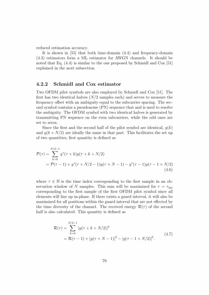
reduced estimation accuracy.It is shown in [55] that both time-domain (4.4) and frequency-domain

(4.3) estimators form a ML estimator for AWGN channels. It should benoted that Eq. (4.4) is similar to the one proposed by Schmidl and Cox [51]explained in the next subsection.

4.2.2 Schmidl and Cox estimator

Two OFDM pilot symbols are also employed by Schmidl and Cox [51]. Thefirst has two identical halves (N/2 samples each) and serves to measure thefrequency offset with an ambiguity equal to the subcarrier spacing. The sec-ond symbol contains a pseudonoise (PN) sequence that and is used to resolvethe ambiguity. The OFDM symbol with two identical halves is generated bytransmitting PN sequence on the even subcarriers, while the odd ones areset to zeros.

Since the first and the second half of the pilot symbol are identical, y(k)and y(k +N/2) are ideally the same in that part. This facilitates the set upof two quantities, first quantity is defined as

P(τ) =

N/2−1∑

k=0

y∗(τ + k)y(τ + k +N/2)

= P(τ − 1) + y∗(τ +N/2 − 1)y(τ +N − 1) − y∗(τ − 1)y(τ − 1 +N/2)

(4.6)

where τ ∈ N is the time index corresponding to the first sample in an ob-servation window of N samples. This sum will be maximized for τ = τopt

corresponding to the first sample of the first OFDM pilot symbol since allelements will line up in-phase. If there exists a guard interval, it will also bemaximized for all positions within the guard interval that are not effected bythe time diversity of the channel. The received energy R(τ) of the secondhalf is also calculated. This quantity is defined as

R(τ) =

N/2−1∑

k=0

|y(τ + k +N/2)|2

= R(τ − 1) + |y(τ +N − 1)|2 − |y(τ − 1 +N/2)|2 .(4.7)

79

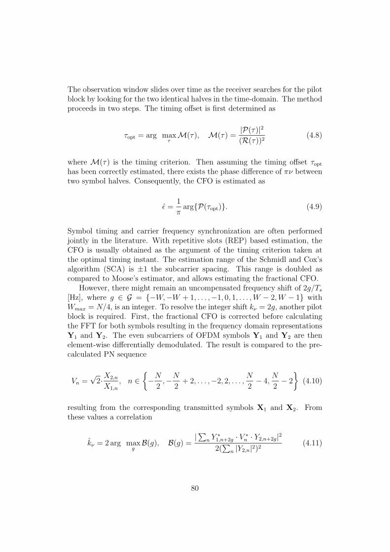
The observation window slides over time as the receiver searches for the pilotblock by looking for the two identical halves in the time-domain. The methodproceeds in two steps. The timing offset is first determined as

τopt = arg maxτ

M(τ), M(τ) =|P(τ)|2(R(τ))2

(4.8)

where M(τ) is the timing criterion. Then assuming the timing offset τopt

has been correctly estimated, there exists the phase difference of πν betweentwo symbol halves. Consequently, the CFO is estimated as

ǫ =1

πarg{P(τopt)}. (4.9)

Symbol timing and carrier frequency synchronization are often performedjointly in the literature. With repetitive slots (REP) based estimation, theCFO is usually obtained as the argument of the timing criterion taken atthe optimal timing instant. The estimation range of the Schmidl and Cox’salgorithm (SCA) is ±1 the subcarrier spacing. This range is doubled ascompared to Moose’s estimator, and allows estimating the fractional CFO.

However, there might remain an uncompensated frequency shift of 2g/Ts[Hz], where g ∈ G = {−W,−W + 1, . . . ,−1, 0, 1, . . . ,W − 2,W − 1} withWmax = N/4, is an integer. To resolve the integer shift kν = 2g, another pilotblock is required. First, the fractional CFO is corrected before calculatingthe FFT for both symbols resulting in the frequency domain representationsY1 and Y2. The even subcarriers of OFDM symbols Y1 and Y2 are thenelement-wise differentially demodulated. The result is compared to the pre-calculated PN sequence

Vn =√

2·X2,n

X1,n

, n ∈{−N

2,−N

2+ 2, . . . ,−2, 2, . . . ,

N

2− 4,

N

2− 2

}(4.10)

resulting from the corresponding transmitted symbols X1 and X2. Fromthese values a correlation

kν = 2 arg maxg

B(g), B(g) =|∑n Y

∗1,n+2g · V ∗

n · Y2,n+2g|22(∑

n |Y2,n|2)2(4.11)

80

that also partially eliminates possible influences from transmission channel, iscalculated. The g that maximizes B(g) delivers the integer frequency offset,so that the total estimated frequency offset is kν + ǫ.

4.2.3 Morelli and Mengali estimator

Morelli and Mengali [52] proposed an extension of Schmidl and Cox algo-rithm (SCA) with a pilot symbol composed of L > 2 identical parts in thetime domain. They are generated by transmitting a pilot sequence on the fre-quency multiples of L/T and setting zeros for the remaining frequencies (seeFig. 4.2). In the sequel, it is referred to as M&M estimator. The main ben-efit over the conventional SCA is an increase of the estimation range whichbecomes ±L/2 the subcarrier spacing. The M&M exploits the correlation

0 50 100 150 200 2500

0.2

0.4

0.6

0.8

1

1.2

subcarrier index

absolu

te v

alu

e o

f th

e p

ilot spectr

um

Transmitted pilot symbol

Received pilot with freq. offset

ν L/T

Figure 4.2: Frequency domain of the transmitted and received pilot symbol.

81

between identical slots of the pilot symbol defined as

r(m) =1

N −mM

N−1∑

k=mM

y(k)y∗(k −mM), 0 ≤ m ≤ P − 1 (4.12)

where M = N/L is the length in sampling interval of each section of thetraining block and P ∈ N is a design parameter. Substituting (4.1) into(4.12) yields

r(m) = ej2πmν/Ld(m) + γ(m) (4.13)

where d(m) , 1N−mM

∑N−1k=mM |s(k)|2 is the real-valued random envelope, and

γ(m) is the noise term defined in [52].By considering the phase differences of the correlation estimate

ϕ(m) = arg{r(m)r∗(m− 1)}, 1 ≤ m ≤ P − 1

≈ 2πν/L+ γI(m) − γI(m− 1)(4.14)

where γI(m) is the imaginary part of γ(m), the best linear unbias estimator(BLUE) of the CFO can be expressed as

νM&M =L

2π

P−1∑

m=1

ωM&M(m)ϕ(m) (4.15)

where the weighting function ωM&M(m) is given by

ωM&M(m) = 3(L−m)(L−m+ 1) − P (L− P )

P (4P 2 − 6PL+ 3L2 − 1). (4.16)

The direct derivation of ωM&M(m) using BLUE principle can be found in [35].The weighting function (4.16) is channel independent. Thus the M&M is theBLUE for any channel. It is shown in [52] that the variance of the M&Mestimator achieves its minimum when P = L/2. It is interesting to noticethat M&M estimator reduces to SCA for L = 2 and P = 1. The M&Mestimates have slightly lower variance than those of SCA. The price to bepaid is an increase in computational complexity, as P angles have to becomputed instead of one for the SCA.

82

4.2.4 Proposed nonlinear least-squares estimator

In the derivation of the proposed NLS estimator, we adopt the pilot symbolhaving a repetitive structure similar to that proposed in [52]. While [52] ap-plies the BLUE concept to the phase differences of the estimated correlationsamples, we use a different approach [6] that relies on the NLS principle inconjunction with the summation-by-parts formula. As a result, we obtaintwo new estimators, the first is the general form for fading channels and theother is its special case for AWGN channel.

Derivation of the generalized NLS estimator

The NLS estimates of {d(m)}P−1m=0 and ν are obtained by solving the following

minimization problem

{d, ν} = arg mind, ν

1

P

P−1∑

m=0

|r(m) − d(m)ej2πmν/L|2. (4.17)

Let

r = [r(0), · · · , r(P − 1)]T

d = [d(0), · · · , d(P − 1)]T

W = diag(1, ej2πν/L, · · · , ej2π(P−1)ν/L

)(4.18)

so that the inner term of (4.17) can be formulated as

J(d, ν) =1

P‖r − Wd‖2 (4.19)

where ‖z‖2 , zHz. Taking the derivative of J(d, ν) with respect to d, yields

∂

∂dJ(d, ν) =

1

P

(−Wr∗ − WHr + 2d

)(4.20)

where (·)T and (·)H denote transpose and complex conjugate transpose, re-spectively. Hence, for any given value of ν, the vector d that minimizes∂∂dJ(d, ν) is d = 1

2{Wr∗ + WHr}, where (·)∗ denotes complex conjugate.

83

Substituting d into J(d, ν), we need to minimize

J(ν) =1

P‖r − 1

2W2r∗ − 1

2r‖2

=1

2PrHr − 1

2PRe{rTW2∗r}

(4.21)

or, equivalently, to maximize the last term of (4.21). Hence, the NLS estimateof the parameter ν can be expressed as

νNLS = arg maxν

Re

{P−1∑

m=0

r2(m)e−j4πmν/L

}(4.22)

which can be efficiently realized by means of Fast Fourier Transform (FFT)with zero padding. This can be done by O(Nf log2Nf ) operations, where Nf

is the number of Fourier bins.

Simplified NLS estimator

A simpler form of (4.22) is obtained by assuming the availability of the phaseof the estimated correlation samples. Let φm = arg{r(m)} denotes the phaseof the correlation estimate. The NLS criterion (4.22) can then be rewrittenas

P−1∑

m=0

|r(m)|2 cos(2φm − 4πmν/L). (4.23)

Setting the derivative of this criterion with respect to ν to zero, we obtain∑P−1m=0m|r(m)|2 sin(2φm − 4πmν/L) = 0. Under the small error approxima-

tion, i.e., sin(2φm−4πmν/L) ≃ (2φm−4πmν/L), the simplified NLS (SNLS)estimator is obtained as

νSNLS =L

2π

∑P−1m=1m|r(m)|2φm∑P−1m=1m

2|r(m)|2. (4.24)

Note that without applying a proper phase unwrapping algorithm, the esti-mation range of the SNLS is limited to ±L/2P .

84

Approximated NLS estimator using summation-by-parts

To make the SNLS independent of any phase unwrapping procedure, thephase increments of the estimated correlation, ∆φm = arg{r(m)r∗(m− 1)},shall be exploited instead of φm. For this purpose, the summation-by-partsformula is proposed. Consider the well known summation-by-parts formula

P−1∑

m=0

∆bmam = bP−1aP−1 − b−1a0 −P−1∑

m=1

bm−1∆am (4.25)

where ∆bm = bm − bm−1 and ∆am = am − am−1. Inspecting (4.25), and thenominator term in (4.24) yields

P−1∑

m=1

m|r(m)|2︸ ︷︷ ︸∆bm

· arg{r(m)}︸ ︷︷ ︸am

= bP−1 arg{r(P − 1)} −P−1∑

m=1

bm−1∆φm

=P−1∑

m=1

(bP−1 − bm−1)∆φm

(4.26)

where ∆b0 = 0, b−1 = 0, arg{r(P − 1)} =∑P−1

m=1 ∆φm. Since b−1 = 0 and∆b0 = 0, one obtains:

bm =m∑

k=1

∆bk =m∑

k=1

k|r(k)|2. (4.27)

Inserting (4.27) into (4.26), and then into (4.24), yields

νANLS =L

2π·∑P−1

k=1 k|r(k)|2∑P−1

m=1 ∆φm −∑P−1m=2

∑m−1k=1 k|r(k)|2∆φm∑P−1

m=1m2|r(m)|2

. (4.28)

Eq. (4.28) can be seen as an approximated version of the NLS (ANLS), whichdoes not require any phase unwrapping procedure as needed for the SNLS.

85

Interesting enough, for the AWGN channel, (4.28) reduces to

νAWGN =3L

2π

P−1∑

m=1

(P − 1)P − (m− 1)m

P (2P − 1)(P − 1)∆φm. (4.29)

Remark I : For the AWGN channel case, the SNLS estimator (4.24) isequivalent to the well known estimator proposed by Fitz [24] and if thesummation-by-parts formula is applied to it, the resulting estimator yields asimilar form as (4.29).

Remark II : Although the ANLS estimator (4.28) is derived based on asingle pilot symbol with L identical parts, the ANLS (with few modifications)can also be used in the case where the multiple identical pilot symbols areemployed.

4.3 Enhancement with Multiple Antennas

Recently, CFO estimation with multiple antennas has increasingly gainedattention since the spatial diversity can be exploited in order to enhancethe estimation performance [56–59]. The diversity combining techniquesfor the time-domain CFO problem (pre-FFT) have been explored in [56]for single-input multiple-output (SIMO) systems using the repeated OFDMsymbols [55]. To utilize the information from all branches, [56] proposed toperform a nonlinear operation before summing up all the signals (see Fig.4.3). This method was also used in the work of [57] and [58]. The accuracyof the CFO estimators using such a combining technique can be consider-ably enhanced. However, these estimators rely on the absolute phase ofthe correlation sum, φm = arg {rs(m)}, and not on the phase difference,∆φm = arg {rs(m)r∗s(m− 1)}, thus they have a limited estimation range.This range can be simply widened using shorter symbols but at the costof reduced estimation accuracy. In this section, it will be shown that theperformance of the ANLS estimator derived in the previous section can beenhanced with antenna diversity combining strategy proposed by [56].

4.3.1 Correlation sum observation

The estimated correlation of the i-th receive antenna is calculated as in (4.12).As the observation, the sum of ri(m) from all receive antennas can be ex-

86

~

1

Nr

~

Correlator

# 1

Correlator

# Nr

CFO

estimator

Tx oscillator Rx oscillator

OFDM

baseband

OFDM

basebandrs(m)

r1(m)

rNr(m)

Tx antenna

Rx antennasNonlinear operation

Figure 4.3: Configuration of CFO estimation with multiple receive antennas.

pressed asNr∑

i=1

ri(m)

︸ ︷︷ ︸rs(m)

= ej2πmν

L

Nr∑

i=1

di(m)

︸ ︷︷ ︸ds(m)

+Nr∑

i=1

γi(m)

︸ ︷︷ ︸γs(m)

(4.30)

where Nr is the number of receive antennas, and rs(m) = |rs(m)|ej arg{rs(m)}

is the sum of the estimated correlation. Without considering the probabilitydensity functions of ds(m) and γs(m), two simple and straightforward esti-mators can be obtained either by performing the simple average (SAV) onφm = arg{rs(m)}

νSAV =L

2πP

P−1∑

m=1

arg{rs(m)}m

(4.31)

or applying the unweighted average (UAV) on ∆φm = arg{rs(m)r∗s(m− 1)}

νUAV =L

2π(P − 1)

P−1∑

m=1

arg{rs(m)r∗s(m− 1)}. (4.32)

The SAV estimator has an estimation range limited to ±L/2P . This rangecan be extended by increasing L (or reducing M), but at the cost of thereduced accuracy. On the other hand, if the UAV is used the range can beenlarged. However, there is no guarantee regarding its estimation accuracysince the ∆φm are not properly weighted.

87

The ANLS (4.28) and AWGN (4.29) estimators derived in the previoussection, can be used in this context (see [6]) by simply replacing the |r(m)|with |rs(m)| and the arg{r(m)r∗m− 1} with arg{rs(m)r∗sm− 1}.

4.4 Simulation Results

We evaluate the proposed estimator in the frequency-selective channels andassume that time synchronization is perfectly achieved. The simulationsare divided into two parts. The first set of simulations are carried out forOFDM with single transmit and single receive antenna in both quasi-static(static over one OFDM symbol) and time-varying channels. The second setof simulations is performed for single transmit and multiple receive antennas.In both set of simulations, the following common conditions are used:

1. Only one single OFDM pilot symbol, with repetitive slots (L > 2), isused.

2. The pilot symbols are taken from a QPSK complex constellation.

3. The useful part of an OFDM symbol contains 256 samples (N=256).

4. A cyclic prefix of 30 samples is used (chosen to be longer than thechannel impulse response).

5. A channel bandwidth of 5 MHz and a carrier frequency of 1 GHz areassumed. The sampling interval Ts = T/N is 0.2 µs.

4.4.1 SISO-OFDM

The frequency-selective channels for SISO-OFDM are set up such that thechannel has 15 paths, with path delays of 0, 1, 2, . . . , 14 samples. The am-plitude Ai of the i-th path varies independently of the others according toa Rayleigh distribution with exponential power delay profile, i.e., E{A2

i } =exp{−i/5}. The phase of each path is uniformly distributed on the interval[0, 2π).

Fig. 4.4 illustrates the average estimate E{ν} of different estimators asa function of the true offset ν for SNR = 20 dB. The parameters P = 16and L = 15 are used. The ideal curve is given as a reference. The channelis static (BDT = 0). It can be seen that the estimation range of the ANLSis about ±L/2 the subcarrier spacing which is similar to that of the M&M

88

and NLS estimators. On the other hand, without phase unwrapping, theestimation range of SNLS is limited to ±1. Similar results are obtained withtime-varying channel BDT = 0.01.

−8 −6 −4 −2 0 2 4 6 8−10

−8

−6

−4

−2

0

2

4

6

8

10

ν

Avera

ge e

stim

ate

SNLS

ANLS

M&M

ideal

Figure 4.4: Average estimate E{ν} vs. ν of the ANLS, SNLS, M&M esti-mators, SISO case, with L = 16, P = 15, SNR = 20 dB.

Fig. 4.5 shows the mean square estimation error (MSE) as a function ofSNR. The carrier frequency offset is set to ν = 0.01 such that it falls withinthe estimation range of SNLS which is limited to only ±L/2P . L varies from8, 16, and 32. The design parameter P is set to P = L/2 and P = L− 1 foreach value of L. The CRLB for SISO case is given as

CRLB(ν) =1

2π2

3 · SNR−1

N(1 − 1/N2)(4.33)

for comparison. It can be seen that with the static channels the performancesof the ANLS and M&M estimators are similar and close to the CRLB. Theperformance of both estimators increase as P and L increase. In time-varyingscenarios, the curves exhibit floors due to the coherence loss between thesegments of the pilot symbol. The performances tend to become worse as mincreases. This implies that optimal value of m should be decreased with theDoppler spread of the fading channel.

89

−5 0 5 10 1510

−6

10−5

10−4

10−3

SNR (dB)

MS

E

CRB

SNLS

ANLS

M&M

BDT=0.025

BDT=0

L = 8P = 4

−5 0 5 10 1510

−6

10−5

10−4

10−3

SNR (dB)

MS

E

CRB

SNLS

ANLS

M&M

BDT = 0

BDT = 0.025

L = 8P = 7

−5 0 5 10 1510

−6

10−5

10−4

10−3

SNR (dB)

MS

E CRB

SNLS

ANLS

M&M

BDT = 0.025

BDT = 0L = 16P = 8

−5 0 5 10 1510

−6

10−5

10−4

10−3

10−2

SNR (dB)

MS

E

CRB

SNLS

ANLS

M&M

BDT = 0.025

BDT = 0

L = 16P = 15

−5 0 5 10 1510

−7

10−6

10−5

10−4

10−3

10−2

10−1

SNE (dB)

MS

E

CRB

SNLS

ANLS

M&M

L = 32P = 16

BDT = 0.025

BDT = 0

−5 0 5 10 1510

−7

10−6

10−5

10−4

10−3

10−2

10−1

100

SNR (dB)

MS

E

CRB

SNLS

ANLS

M&M

BDT=0.025

BDT = 0L = 32P = 31

Figure 4.5: MSE vs. SNR of the ANLS, SNLS, M&M estimators, L = 16and 32, with P = L/2 and L−1, for ν = 0.01.

4.4.2 SIMO-OFDM

Fig. 4.6 illustrates the average estimate E{ν} of different estimators as afunction of the true offset ν for SNR = 20 dB and BDT = 0 (static channel).The ideal curve is given as a reference. It is confirmed that the estimationranges of those approaches which exploit the phase difference (ANLS, AWGN,

90

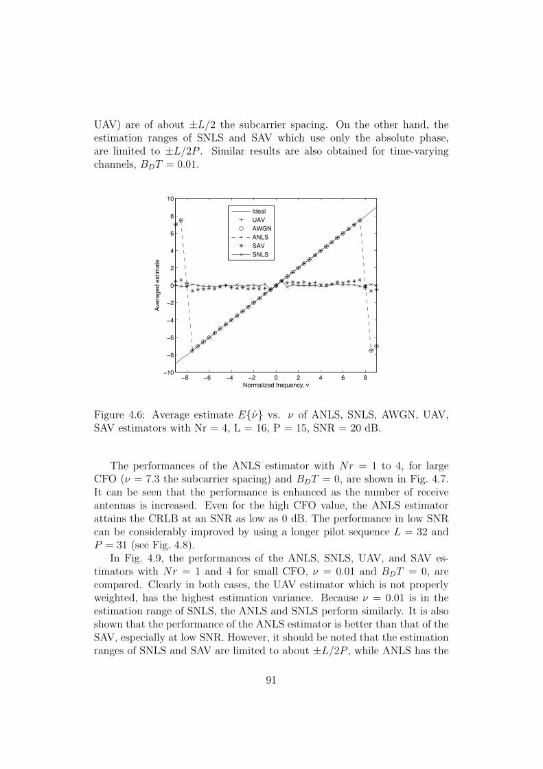
UAV) are of about ±L/2 the subcarrier spacing. On the other hand, theestimation ranges of SNLS and SAV which use only the absolute phase,are limited to ±L/2P . Similar results are also obtained for time-varyingchannels, BDT = 0.01.

−8 −6 −4 −2 0 2 4 6 8−10

−8

−6

−4

−2

0

2

4

6

8

10

Normalized frequency, ν

Avera

ged e

stim

ate

Ideal

UAV

AWGN

ANLS

SAV

SNLS

Figure 4.6: Average estimate E{ν} vs. ν of ANLS, SNLS, AWGN, UAV,SAV estimators with Nr = 4, L = 16, P = 15, SNR = 20 dB.

The performances of the ANLS estimator with Nr = 1 to 4, for largeCFO (ν = 7.3 the subcarrier spacing) and BDT = 0, are shown in Fig. 4.7.It can be seen that the performance is enhanced as the number of receiveantennas is increased. Even for the high CFO value, the ANLS estimatorattains the CRLB at an SNR as low as 0 dB. The performance in low SNRcan be considerably improved by using a longer pilot sequence L = 32 andP = 31 (see Fig. 4.8).

In Fig. 4.9, the performances of the ANLS, SNLS, UAV, and SAV es-timators with Nr = 1 and 4 for small CFO, ν = 0.01 and BDT = 0, arecompared. Clearly in both cases, the UAV estimator which is not properlyweighted, has the highest estimation variance. Because ν = 0.01 is in theestimation range of SNLS, the ANLS and SNLS perform similarly. It is alsoshown that the performance of the ANLS estimator is better than that of theSAV, especially at low SNR. However, it should be noted that the estimationranges of SNLS and SAV are limited to about ±L/2P , while ANLS has the

91

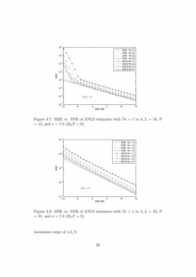
−10 −5 0 5 10 1510

−7

10−6

10−5

10−4

10−3

10−2

10−1

100

SNR (dB)

MS

E

CRB Nr=1

CRB Nr=2

CRB Nr=3

CRB Nr=4

ANLS Nr=1

ANLS Nr=2

ANLS Nr=3

ANLS Nr=4

BDT = 0

Figure 4.7: MSE vs. SNR of ANLS estimator with Nr = 1 to 4, L = 16, P= 15, and ν = 7.3 (BDT = 0).

−10 −5 0 5 10 1510

−7

10−6

10−5

10−4

10−3

SNR (dB)

MS

E

CRB Nr = 1

CRB Nr = 2

CRB Nr = 3

CRB Nr = 4

ANLS Nr = 1

ANLS Nr = 2

ANLS Nr = 3

ANLS Nr = 4

BDT = 0

Figure 4.8: MSE vs. SNR of ANLS estimator with Nr = 1 to 4, L = 32, P= 31, and ν = 7.3 (BDT = 0).

maximum range of ±L/2.

92

−10 −5 0 5 10 1510

−7

10−6

10−5

10−4

10−3

10−2

SNR (dB)

MS

E

ANLS Nr=1

SNLS Nr=1

SAV Nr=1

UAV Nr=1

CRB Nr=1

ANLS Nr=4

SNLS Nr=4

SAV Nr=4

UAV Nr=4

CRB Nr=4Nr = 1

Nr = 4BDT = 0

Figure 4.9: MSE vs. SNR of ANLS, SNLS, SAV, UAV estimators with Nr= 1 and 4, and ν = 0.01 (BDT = 0).

Fig. 4.10 shows the error floor effect caused by the Doppler spread of theANLS and UAV estimators withNr = 1 and 4 for ν = 7.3. It can be observedthat the error floor effect reduces as the number of receive antennas increases.However, the unweighted UAV still performs poorer than the proposed ANLSestimator. For Nr = 4, the estimation variance of the ANLS estimator isalready close to the CRLB.

Fig. 4.11 compares the performances of the ANLS, SNLS, and SAV esti-mators in time-varying channel for small CFO, ν = 0.01. Since |ν| < L/2P ,it can be seen that the performances of the ANLS and SNLS are similar andbetter than that of the SAV estimator especially at low SNR. Similar to thelarge CFO case (see Fig. 4.10), the error floor effect reduces as the numberof receive antennas increases.

93

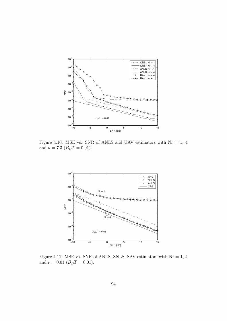
−10 −5 0 5 10 1510

−7

10−6

10−5

10−4

10−3

10−2

10−1

100

101

SNR (dB)

MS

ECRB Nr = 1

CRB Nr = 4

ANLS Nr =1

ANLS Nr = 4

UAV Nr = 4

UAV Nr = 1

BDT = 0.01

Figure 4.10: MSE vs. SNR of ANLS and UAV estimators with Nr = 1, 4and ν = 7.3 (BDT = 0.01).

−10 −5 0 5 10 1510

−7

10−6

10−5

10−4

10−3

10−2

SNR (dB)

MS

E

SAV

SNLS

ANLS

CRB

BDT = 0.01

Nr = 1

Nr = 4

Figure 4.11: MSE vs. SNR of ANLS, SNLS, SAV estimators with Nr = 1, 4and ν = 0.01 (BDT = 0.01).

94

4.5 Summary

The classical CFO estimators for OFDM signals have been discussed. Theproposed estimator, which relies on the nonlinear least-squares principle inconjunction with the summation-by-parts formula, has shown to be muchsimpler to derive (as compared to M&M estimator) and has the maximumpossible estimation range of about ±L/2 without an additional phase un-wrapping algorithm which is needed for most of the classical estimators. Theestimation variance of the proposed estimator however suffers from the errorfloor effect caused mainly by Doppler spread. This effect can be reduced byintroducing the receive antenna diversity concept.

95

Chapter 5

Frequency Estimation: Radar

and Array Processing

This chapter relates the problem of frequency estimation in the syntheticaperture radar (SAR) and array processing contexts to the problem of car-rier frequency offset estimation introduced in the previous chapters. It willbe seen that the signal models for Doppler centroid estimation in SAR andthe direction-of-arrival (DOA) estimation in array processing applicationsare similar to that of the classical one, hence most of the already existing in-cluding the proposed frequency estimation algorithms can be applied. A newconcept of the integrated GPS/INS for DOA estimation is also introduced inthis chapter.

5.1 Doppler Centroid Estimation: SAR

Estimation of the Doppler frequency is a fundamental operation in radardata processing. Weather radar and moving-target indication radar exploitthe Doppler shift of each radar return to measure the velocity of scatterers.In the image formation algorithm for SAR, two-dimensional matched filter-ing (the range compression and azimuth compression) is the fundamentaloperation. This can be done either by two one-dimensional processing steps,Range-Doppler approach, or implementing a truly two-dimensional process-ing step usually implemented in frequency domain, where the matched fil-

96

tering performs the azimuth compression as well as the range migration cor-rection.

For the range-Doppler approach, during the azimuth compression therange compressed data is correlated with the replica of the azimuth chirp,which depends on the phase history of the SAR sensor relative to the terrainbeing imaged during the interval of observation. The phase history can beapproximated by a truncated Taylor series expansion which contains the firstand second order derivatives of phase at the center of the synthetic aperture.For many applications, especially when the SAR carrier platform exhibitstime varying attitude errors, the first order derivative, known as Dopplercentroid frequency, fDC must be estimated from the measurement data.

The Doppler centroid can also be seen as a measure of the effective an-tenna squint angle. It is used to adjust the bandpass characteristic of theazimuth compression filter to the location of the signal spectrum. An in-accurate Doppler centroid not only affects resolution and the signal-to-noiseratio, but also allows aliased azimuth frequency components to fall within thepassband of the compression filter, and thus reduces the signal-to-ambiguityratio [60,61].

The Doppler centroid (the Doppler shift of a target positioned in theantenna boresight direction) is an important parameter in relation to azimuth(along track) SAR processing. For an airborne radar where the antenna ispointed perpendicular to the flight line, the Doppler centroid is ideally zero.However, if the antenna is off-set in angle (squinted), which might be dueto desired or undesired yaw or if a satellite SAR orbiting a rotating earth isconsidered, then fDC will be different from zero [62].

In principle, it is possible to calculate the Doppler centroid from orbit andattitude data, but measurement uncertainties on these parameters (primar-ily attitude) will limit the accuracy. These errors will eventually degrade theperformance of the processing, especially w.r.t. signal-to-noise ratio, side-lobe, and ambiguity levels. Alternatively, Doppler centroid can be estimatedfrom the received complex echo data. This has been done in the along-trackdimension [61–63]. The time domain correlation-based Doppler centroid esti-mator has been used by Madsen [62] which was originally applied to spectralestimation in other field [64]. In [65, 66], various type of Kalman filters andsmoothers were used to improve the Doppler centroid estimates which canbe determined by correlation-based techniques.

If the azimuth data y(k) = y(kT ) is a stochastic process, its correlationfunction of two samples separated by m-lag is given by

ry(m) = E{y(k)y∗(k −m)} (5.1)

97

and the power spectrum is given by

Sy(f) = F{ry(m)} =∞∑

m=−∞r(m)e−j2πmTf (5.2)

or

ry(m) = F−1{Sy(f)} = T

∫ 1/2T

−1/2T

S(f)ej2πmTfdf. (5.3)

If the azimuth power spectrum is shifted by fDC , we have

S(f) = Sy(f − fDC). (5.4)

For frequency domain approaches, this shift is estimated directly in the az-imuth frequency domain from an estimated azimuth power spectrum. How-ever, for the time domain interpretation the corresponding correlation func-tion can be written as

r(m) = ej2πmTfDC · ry(m). (5.5)

This result is the basis of the time-domain estimation of the Doppler centroid.It is seen that the phase of the correlation function is directly related tothe Doppler centroid. Therefore, one can by estimation of the correlationfunction r(m), arrive at an estimate of the Doppler centroid, which can becalculated using either unbiased (3.56) or biased (3.57) form of the correlationestimates. Madsen used azimuth window size of m = 1 as the primaryDoppler centroid estimator.

Notice that (5.5) has a similar form as (3.55), and hence the nonlinearleast-squares concept (4.17)-(4.24) followed by the summation-by-parts for-mula can be again directly applied. This yields an estimator of a similarform as (3.69). The CRLB can be obtained in the same way as derived inthe Appendix (A.2.1).

5.2 DOA Estimation: Array Processing

Consider the array ofM identical sensors uniformly spaced on a line, depictedin Fig. 5.1. Such an array is commonly referred as a uniform linear array

98

far-field planar

wavefronts

d

2d

3d

( 1)M d

0

2

3

( 1)M

DO

A e

stim

atio

n a

nd s

patia

l pro

cessin

g

1( )x t

4 ( )x t

2 ( )x t

3( )x t

( )Mx t

( )y t

sind

c

Figure 5.1: Basic geometry of a uniform linear array (ULA) of a single source.

(ULA). Let d denote the distance between two consecutive sensors, and let θdenotes the direction of arrival (DOA) of the narrowband signal illuminatingthe array, as measured with respect to the normal line of sensors. Then underthe planar wave hypothesis (far-field), no angular spread, and the assumptionthat the first sensor in the array is chosen as the reference point, the array’soutput vector may be written as

x(t) = a(θ)s(t) + n(t) (5.6)

where x(t) = [x1(t), · · · , xM(t)]T , a(θ) = [1, e−jωcτ2 , · · · , e−jωcτM ]T , and n(t) =[n1(t), · · · , nM(t)]T . The delay of the wavefront to the m-th sensor is

τm = (m− 1)d sin θ

c, for θ ∈

[−π

2,π

2

](5.7)

where c is the speed of light, and m is the sensor’s index. Inserting (5.7) intoa(θ) results in

a(θ) =[1, e−jωcd sin θ/c, · · · , e−j(M−1)ωcd sin θ/c

]T. (5.8)

The restriction of θ to lie in the interval [−π/2, π/2] is a limitation of ULAs:two sources at locations symmetric with respect to the array line yield iden-

99

tical sets of delays and hence cannot be distinguished from another. Inpractice, this ambiguity is eliminated by using sensors that only pass signalswhose DOAs are in [−π/2, π/2] .

Let λ denote the signal wavelength

λ = c/fc, fc = ωc/2π. (5.9)

By defining

fs = fcd sin θ

c=d sin θ

λ(5.10)

and

ωs = 2πfs = ωcd sin θ

c(5.11)

yields

a(θ) =[1, e−jωs , · · · , e−j(M−1)ωs

]T(5.12)

where ωs is known as the spatial frequency. Note that a(θ) is a Vandermondevector which is completely analogous with the vector made from the uniformsamples of the sinusoidal signal {e−jωst}. The vector a(θ) can be uniquelydefined (i.e., there is no spatial aliasing) if and only if ωs is constrained as

|ωs| ≤ π or |fs| ≤1

2⇔ d| sin θ| ≤ λ

2. (5.13)

This condition is satisfied if d ≤ λ/2, which implies that the spatial samplingperiod d should be smaller than half of the signal wavelength.

The extension of (5.6) to the case of multiple sources is straightforward.Since the sensors in the array were assumed to be linear elements, a directapplication of the superposition principle leads to the following model of thearray

x(t) = As(t) + n(t)

= [a(θ1), · · · , a(θK)]

s1(t)

...sK(t)

+ n(t)

(5.14)

where θk is the DOA of the k-th source, and sk(t) is the signal correspondingto the k-th source.

100

Eq. (5.6) and (5.14) are similar to the models used in the non-fadingsinusoidal signal cases, therefore most of the (temporal) frequency estimationmethods for sinusoidal signals can be used for the DOA estimation problem.

In practice, estimating the DOA in the presence of local scattering is morecomplicated. This is often seen in wireless mobile communications since thesources may appear to be spatially distributed due to local scattering aroundthe mobile unit. Local scattering at the source causes signals from a singlesource to arrive via different paths and at different angles. The point sourceis now said to exhibit angular spread. Angular spread manifests itself vialoss of spatial coherence of the signal across the receiver array. Hence, thisscenario is also referred to as imperfect spatial coherence [67]. Imperfectspatial coherence is also encountered in sonar systems when the propagationmedium is randomly inhomogeneous [67].

Model formulation

In this section, a single scattered source model for DOA estimation problem isdeveloped. The earlier works for single scattered source can be found in [68–70] and [71] for multiple scattered sources. In order to obtain a proper model,it is assumed that the delay spread caused by the multipath propagation issmall compared to the inverse bandwidth of the signal so that the narrowbandassumption still holds even in the presence of scattering. The noise freenarrowband signal arriving at the m-th sensor of an M -element ULA can bewritten as

xm(t) =s(t)√L(t)

L(t)∑

i=1

gi(t) exp {−j2π∆(m− 1) sin(θ + φi(t))} (5.15)

where L(t) is the number of scattered rays, ∆ is the sensor spacing in wave-lengths, θ is the angle to be estimated, gi(t) is the complex amplitude ofthe i-th arrival, and φi(t) is its angular spread. If the angular spread issmall (the scattering occurs near the source and the array is in the far-field),sin(θ + φi(t)) ≈ sin(θ) + cos(θ)φi(t). Hence, the noisy array output can beapproximated by

xm(t) = s(t)um(t) exp {−j2π∆(m− 1) sin θ} + nm(t) (5.16)

101

where nm(t) is the additive noise at the k-th sensor, and um(t) models theperturbations due to the spatial scattering, and is given by

um(t) = µ+∑

n

gn(t) exp{j2π∆(m− 1) cos(θ)φn(t)} (5.17)

where µ denotes the complex gain of the dominant path (at the nominalangle), if it is exist. The following assumptions are made in order to obtaina proper model

AS1) The amplitudes, gn(t), and the angular deviation, φn(t), are iid inboth n and t, i.e., spatially and temporally white, zero-mean and mutuallyindependent.

AS2) The angular deviations are stationary and symmetrically distributedaround zero.

AS3) The narrowband signal s(t) is deterministic and unknown.AS4) Additive noise is temporally and spatially iid, zero-mean complex

Gaussian and circular.Under assumptions AS1)-AS2) and assuming that the number of rays,

L(t), is large, [u1(t), · · · , uM(t)] can be modeled (using central limit theorem)as a Gaussian M -variate process. The spatial correlation is given by

Ru(k, l) = E{uk(t)u∗l (t)} = |µ|2 + σ2gRφ(k, l) (5.18)

where σ2g is the power of the scattered paths and

Rφ(k, l) = E{exp(j2π∆(k − l) cos(θ)φ)}. (5.19)

The covariance of the array outputs is stationary in space but not in time(since s(t) is not assumed to be a constant modulus), and is given by

Rx(k, l; t) = E{xk(t)x∗l (t)}= |s(t)|2[|µ|2 + σ2

gRφ(k, l)]ejωo(k−l) + σ2

nδ(k − l)(5.20)

where ωo = 2π∆ sin θ is the nominal frequency, and σ2n is the variance of the

additive noise. Under AS2), Rφ(k, l) is real-valued.

102

For a Rayleigh channel (µ = 0), the correlation model reduces to

Rx(k, l; t) = |s(t)|2σ2gRφ(k, l)e

jωo(k−l) + σ2nδ(k − l). (5.21)

If φ is uniformly distributed, then Rφ(k, l) = sinc(2π∆(k − l) cos θ), if φ hasGaussian distribution, then Rφ(k, l) = exp(−[2π∆(k − l) cos(θ)σφ]

2/2).The averaged (over N the snapshots) spatial correlation matrix is esti-

mated as

Rx(k, l) =1

N

N∑

t=1

xk(t)x∗l (t), k, l = 1, . . . ,M. (5.22)

Using the following statistic yields

r(m) =1

M −m

M−m∑

k=1

Rx(k +m, k), m = 0, . . . ,M − 1. (5.23)

These correlation coefficients are thus obtained after applying the so-calledredundancy averaging technique to the covariance matrix estimate. It hasbeen shown in [71] that r(m) converges in mean-square to

r(m) = P · ru(m)︸ ︷︷ ︸d(m)

ejωom + σ2nδ(m) (5.24)

where P = 1N

∑Nt=1 |s(t)|2, and ru(m) , ru(k, l).

Notice that (5.24) has a similar form as (3.55), and hence the nonlinearleast-squares concept (4.17)-(4.24) followed by the summation-by-parts for-mula can be again directly applied. This yields an estimator of a similarform as (3.69). The CRLB can be obtained in the same way as derived inthe Appendix (A.2.1).

5.3 DOA Tracker: GPS/INS Integration

In this section, a new concept for DOA tracking via GPS/INS integration isintroduced. Typically, algorithms for tracking of the DOA for a particularsatellite shall properly handle the interferences from other satellites, whichcan be complicated. Ignoring these interferences will lead to a significant

103

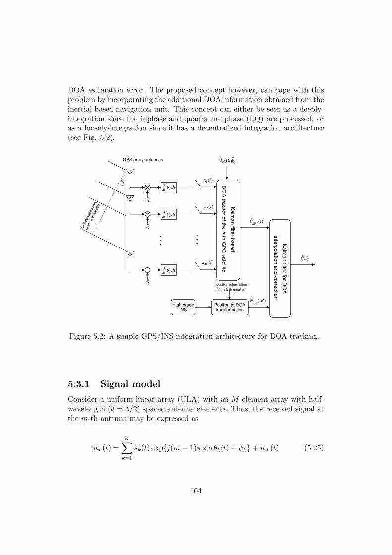
DOA estimation error. The proposed concept however, can cope with thisproblem by incorporating the additional DOA information obtained from theinertial-based navigation unit. This concept can either be seen as a deeply-integration since the inphase and quadrature phase (I,Q) are processed, oras a loosely-integration since it has a decentralized integration architecture(see Fig. 5.2).

1

2

M

0( )

Tdt

*kc

0( )

Tdt

0( )

Tdt

*kc

*kc

1( )x i

2 ( )x i

( )Mx i

Kalm

an filte

r based

DO

A tra

cke

r of th

ek-th

GP

S s

ate

llite

Kalm

an filte

r for D

OA

inte

rpola

tion a

nd c

orre

ctio

n

ˆ ˆ( ),k kd i

ˆ ( )gps i

High gradeINS

GPS array antennas

Position to DOAtransformation

ˆ ( )ins iR

ˆ( )i

position information

of the k-th satellite

k

far-

field

wave

fronts

ofth

ek-

thsa

telli

te

Figure 5.2: A simple GPS/INS integration architecture for DOA tracking.

5.3.1 Signal model

Consider a uniform linear array (ULA) with an M -element array with half-wavelength (d = λ/2) spaced antenna elements. Thus, the received signal atthe m-th antenna may be expressed as

ym(t) =K∑

k=1

sk(t) exp{j(m− 1)π sin θk(t) + φk} + nm(t) (5.25)

104

where K is the number of sources (satellites), θk(t) is the azimuthal DOAof the k-th sources, φk is the carrier phase which is uniformly distributed in[0, 2π], sk(t) =

∑∞i=−∞ dk(i)ck(t−iT−τk), dk(t) is the transmitted data, ck(t)

denotes the spreading sequence waveform, nk(t) is the additive white Gaus-sian noise, τ and T are the time delay and the symbol interval, respectively.The received signal may be written in a vector form as

y(t) = A(θ(t))S(t) + n(t) (5.26)

where

• y(t) = [y1(t), y2(t), · · · , yM(t)]T is an M × 1 vector of the receivedsignals at time t.

• θ(t) = [θ1(t), θ2(t), · · · , θK ]T is the source DOA parameter vector.

• A(θ(t)) is the array response matrix which is determined by the DOAof signals. The k-th column of A(θ(t)) is defined as the array re-sponse vector associated with the k-th source and is given by a(θk(t)) =[1, e−jπ sin θk(t), · · · , e−jπ(M−1) sin θk(t)]T .

• S(t) = diag[s1(t)ejφ1 , s2(t)e

jφ2 , · · · , sK(t)ejφK ].

• n(t) = [n1(t), n2(t), · · · , nM(t)]T is an M × 1 additive noise vector,which is assumed to be spatially and temporally white Gaussian.

The received signals are despread by the users’ own spreading sequencesfor each of the antenna elements. Therefore, the k-th users’ despread andsampled array vector signal, xk(i) may be expressed as

yk(i) = dk(i)a(θk(i))ejφk +

K∑

l=1, l 6=kψkldl(i)a(θl(i))e

jφl + nk(i) (5.27)

where the cross-correlation of the spread sequence, ψkl may be defined asψkl ,

∫ T0ck(t)cl(t)dt when the time delay of all users are zero and nk(i) is

the despread noise signal vector whose covariance matrix is σ2nI. The outputs

are then multiplied by a conjugate of the transmitted data estimate d∗k(i) and

carrier phase estimate e−jφk to remove the effect of dk(i) and φk. With the

assumption that d∗k(i) = dk(i) and φk = φk, yk(i)d∗k(i)e

−jφk can be written

105

as

yk(i) = yk(i)d∗k(i)e

−jφk

= a(θk(i)) + d∗k(i)e−jφk

K∑

l=1, l 6=kψkldl(i)a(θl(i))e

jφl + d∗k(i)e−jφknk(i)

= a(θk(i)) + αk(i) + nk(i)

(5.28)

where αk(i) is a vector containing the interference of the despread signal ofthe k-th satellite, and nk(i) represents the noise vector with the unchangedstatistical properties (see Appendix A.1.4).

5.3.2 GPS DOA tracking via extended Kalman filter

In order to track the DOA of the k-th satellite, θk(i), an extended Kalmanfilter (EKF) is used. The Kalman filtering algorithm is readily formulated inAppendix B.

State space model

For simplicity, the index k indicating the satellite number is omitted. Theθ(i) is modeled as a random walk process.

xi+1 = Axi + wi[θgps(i+ 1)

θgps(i+ 1)

]=

[1 10 1

] [θgps(i)

θgps(i)

]+

[0

wθgps(i)

].

(5.29)

Observation model

The cross-correlation (interference) term, αk(i), contributed to the despreadsignal is ignored and only the measurement noise is considered. A simple

106

observation model can be written as

yi = h(xi) + vi

Re{y1(i)}Re{y2(i)}

...Re{yM(i)}Im{y1(i)}Im{y2(i)}

...Im{yM(i)}

=

cos(0)cos(−1π sin θgps(i))

...cos(−(M − 1)π sin θgps(i))

sin(0)sin(−1π sin θgps(i))

...sin(−(M − 1) sin θgps(i))

+

Re{n1(i)}Re{n2(i)}

...Re{nM(i)}Im{n1(i)}Im{n2(i)}

...Im{nM(i)}

(5.30)

where Re{ym(i)} and Im{ym(i)} are respectively the real and imaginary partof ym(i) at the m-th antenna. Re{nm(i)} and Im{nm(i)} are respectively thereal and imaginary part of nm(i) at the m-th antenna. h(·) is the nonlinearmapping between yi and xi.

The EKF requires the linearized observation matrix (Jacobian matrix)which can be obtained by

H(i) =∂

∂xih(xi)|xi=x

−

i

=

0 0

1π cos θ−gps(i) sin(−1π sin θ−gps(i)) 0...

...

(M − 1)π cos θ−gps(i) sin(−(M − 1)π sin θ−gps(i)) 00 0

−1π cos θ−gps(i) cos(−1π sin θ−gps(i)) 0...

...

−(M − 1)π cos θ−gps(i) cos(−(M − 1)π sin θ−gps(i)) 0

.

(5.31)

The linearized observation model is then

yi = H(i)xi + vi. (5.32)

Since the cross-correlation matrix is unknown and ignored, therefore, one can

107

expect bias errors embedded in the output estimates, θ(i).

5.3.3 GPS/INS integration for DOA tracking

The outputs from the array-GPS DOA tracker, θgps(i), will be fused with

the DOA estimates obtained from the INS unit, θins(iR), via an additionalKalman filter. This approach may be comparable to the well known loosely-coupled GPS/INS integration [72,73]. Assuming that the INS provides accu-rate position estimates for a sufficiently long period of time and the satellites’positions are available to the INS so that the INS can use this information totransform its position into the DOA. The array-GPS DOA tracker outputsthe DOA estimates at a much higher rate than that of the INS (∼ 100− 200Hz), therefore, the integration filter (Kalman filter) will complete the wholeiteration (prediction and correction loops) only when the DOA from INS isavailable otherwise it will only run in the prediction loop. The outputs ofthe array-GPS DOA tracker are erroneous since the cross-correlations are notconsidered. However, by fusing the erroneous estimates with the DOA froma high grade INS unit, the error can be significantly reduced.

The state space model is defined as

xi+1 = Axi + wi[∆θ(i+ 1)

∆θ(i+ 1)

]=

[1 10 1

] [∆θ(i)

∆θ(i)

]+

[0

w∆θ(i)

].

(5.33)

Since the difference between the reliable DOA obtained from INS and DOAestimates obtained from the array-GPS, is used as the measurement. Thesimple linear observation model can be obtained as

yi = Hxi + vi[θins(i) − θgps(i)

]=[

1 0] [ ∆θ(i)

∆θ(i)

]+[v(i)

].

(5.34)

The integrated DOA estimate, θ(i), is obtained by (see also Fig. 5.3)

θ(i) = θgps(i) + ∆θ(i). (5.35)

108

Integration

FilterINS-DOA

Array-GPS

DOA tracker

-

+

ˆ( )i( )ins i

( )gps i ˆ( )i

Figure 5.3: GPS/INS integration scheme.

5.3.4 Simulation results

For simulation purpose, the direction-of-arrivals of the GPS signals are gen-erated randomly following the sinusoidal functions. The PN-sequences areused to generate the transmitted and received GPS signals. The followingassumptions are also assumed in the simulations.

• 8 GPS linear array antennas are used.

• The data bits are known and can be removed from the received signal.

• Maximum of 12 GPS satellites are seen by all antennas.

• The array-GPS outputs DOA estimates 100 times faster than INS.

• High quality INS is available.

• Calibration and synchronization are assumed to be perfect.

Fig. 5.4 shows the DOA tracking ability of the array-GPS based DOA trackerwith and without INS aiding. It can be seen that if the cross-correlation orinterference term is ignored and not compensated for, the DOA estimationerror is large. However, by using the proposed GPS/INS integration conceptfor DOA tracking, this error can be significantly reduced. The quality of theINS will of course play an important roll in reducing the estimation error.

109

0 2000 4000 6000 8000 10000−0.02

0

0.02

0.04

0.06

0.08

0.1

0.12

0.14

Iteration

DO

A e

stim

ate

s o

f th

e k

th s

ate

llite

(ra

d)

Non−integrated GPSDOA estimates

Integrated GPS/INSDOA estimates

True DOA

GPS output rate

INS output rate= 100

0 2000 4000 6000 8000 10000−0.04

−0.03

−0.02

−0.01

0

0.01

0.02

0.03

0.04

0.05

Iteration

DO

A e

stim

ation e

rror

of th

e k

th s

ate

llite

(ra

d)

Non−integrated GPSDOA estimation error

Integrated GPS/INSDOA estimation error

GPS output rate

INS output rate= 100

Figure 5.4: DOA tracking via GPS/INS integration.

110

5.4 Summary

This chapter shows that the problem of frequency estimation can also be seenfrom SAR (Doppler centroid estimation) and array processing (direction-of-arrival estimation) point of view. The formulations of the problem in bothcases present finally similar expression as obtained from the carrier frequencyoffset estimation problem in communication systems.

The integrated GPS/INS DOA estimation problem is also considered inthis chapter. It is shown that an additional DOA information can be used toreduce the GPS-alone DOA estimation errors caused by the uncompensatedcross-correlation of GPS signals arriving from other directions.

111

Chapter 6

Conclusions and Future Works

6.1 Conclusions

The performance of communication systems for both single-carrier and multi-carrier (i.e., OFDM) transmission schemes, depend on the signal quality seenby the receiver. The ideal signal integrity is only obtained when the systemimpairment such as CFO is eliminated from the system. On the other hand,the performance of Doppler radar systems depend on how accurately andprecisely the Doppler frequency is extracted from the echo’s signal. Theserequirements demand properly designed frequency estimation algorithms. Inthis thesis, issues related to frequency estimation are addressed. In particu-lar, after introduction of the single-carrier, multi-carrier OFDM systems, andthe analysis of the effects of CFO errors, new data-aided frequency estimationalgorithms have been derived and analyzed. It has been shown in the laterchapter that these proposed algorithms can be easily extended to use in theDoppler radar and array processing applications. The main contributions ofthis thesis include:

Single-carrier case

• Closed-form quadratic interpolation function for the frequency estima-tion using periodogram has been derived. It significantly reduces theamount of zero-padding required by the FFT-periodogram in order toattain the CRLB.

112

• The modified Kay’s estimator, which solves the problem of high thresh-old behavior in the original Kay’s estimator, has been proposed. Thiscomes at the price of a narrower estimation range, however, for a givenestimation range the modified Kay’s estimator can provide a muchlower threshold than the original one.

• The summation-by-parts formula (weight transformation formula) isapplied to extend the estimation range of the original Fitz’s estima-tor which leads to the modified Fitz’s estimator. The original Fitz’sestimator has a very narrow estimation range when operated in theoptimal mode. This problem is usually overcome by applying a properphase unwrapping algorithm, however at the price of high computa-tional complexity.

• An approximated maximum likelihood frequency estimator based onthe absolute phase information of the autocorrelation estimates, is pro-posed. The weight transformation formula is applied to the proposedestimator resulting in the transformed proposed estimator which has asimilar performance as the original one but with the estimation rangeextended to the maximum. The performance of the transformed pro-posed estimator is also shown to be better than that of the well knownM&M estimator.

• By using the nonlinear least-squares principle in conjunction with thesummation-by-parts formula, a new closed-form frequency estimatorwhich can be used to estimate the frequency of signals with fading-induced multiplicative noise has been derived. The estimator requiresneither phase unwrapping algorithm nor additional information aboutthe channel as needed for most of the existing estimators.

• Designed a Kalman filter for frequency estimation of signals with real-valued time-varying amplitude. It can be easily extended for frequencytracking problem.

OFDM case

• The nonlinear least-squares estimator derived for the single-carrier casehas been applied to multi-carrier OFDM signal. The improvement canbe obtained using multiple receive antennas. The error floor effect ofthe estimation variance introduced by the non-delta function of thechannel correlation function can be reduced by using an array of un-correlated receive antennas.

113

Array processing

• The integrated GPS/INS DOA tracker has been proposed. By using theadditional DOA information obtained from INS, the DOA estimationerrors of the GPS-alone tracker can be reduced.

6.2 Future Works

In this work, the problem of frequency estimation in communication andradar related applications has been addressed. Several improved frequencyestimators including a novel closed-form NLS-based frequency estimator havebeen proposed. For future works, a closed-form estimator for the MIMO casemay be derived in the same manner as in the case of SISO and SIMO. Theperformance analysis of these estimators could also be carried out. More-over, for frequency tracking purposes, various types of Kalman filters andsmoothers can be applied on the correlation estimates of the received sig-nals.

Since the proposed NLS-based estimator can also be applied to the Dopplercentroid estimation problem in SAR applications, therefore a justification ofthe proposed estimator by the real SAR data could be of interest.

114

Appendix A

Derivations

A.1 Constant Envelope

A.1.1 Cramer-Rao lower bound

The complex Gaussian pdf is defined as

p(x; ξ) =1

πN det(Cx(ξ))exp

[−(x − µ(ξ))HC−1

x (ξ)(x − µ(ξ))]

(A.1)

where the parameter vector ξ is to be estimated based on the complex datax = [x[0], x[1], . . . , x[N−1]]T and may have components that are real and/orcomplex. However, in this thesis only the real-valued case is considered.

The Cramer-Rao lower bound (CRLB) for a complex Gaussian pdf isobtained from the inverse of the Fisher information matrix defined as (seeeq.(15.52) in [74])

[I(ξ)]ij = tr

{C−1x (ξ)

∂Cx(ξ)

∂ξiC−1x (ξ)

∂Cx(ξ)

∂ξj

}+2Re

{∂µH(ξ)

∂ξiC−1x (ξ)

∂µ(ξ)

∂ξj

}

(A.2)for i, j = 1, 2, . . . , p. The derivatives are defined as the matrix or vector ofpartial derivatives, where we differentiate each complex element g = gR+ jgI

115

as∂g

∂ξi=∂gR∂ξi

+ j∂gI∂ξi

.

The equality condition for the CRLB to be efficient is,

∂ ln p(x; ξ)

∂ξ= I(ξ)(g(x) − ξ)

where ξ = g(x) is the efficient estimate of ξ.Consider the signal model defined in (3.1)

y(k) = a exp{j2πf0k} + n(k), 0 ≤ k ≤ N − 1 (A.3)

where a = a exp{jφ} is a constant complex envelope, f0 = F0T is the nor-malized frequency to be estimated, n(k) = nI(k) + jnQ(k) is a zero-meancomplex-valued white Gaussian process with variance σ2. The SNR is de-fined as a2/σ2. Note that a, φ, f0 are deterministic but unknown.

From (A.2), we have

[I(ξ)]ij = 2Re

{∂µH(ξ)

∂ξi

1

σ2I∂µ(ξ)

∂ξj

}

=2

σ2Re

{N−1∑

k=0

∂s∗(k)

∂ξi

∂s(k)

∂ξj

} (A.4)

where s(k) = a exp{j2πf0k} = a exp{j(2πf0k + φ)}. The partial derivativesare now

∂s(k)

∂a= exp{j(2πf0k + φ)}

∂s(k)

∂f0

= j2πka exp{j(2πf0k + φ)}

∂s(k)

∂φ= ja exp{j(2πf0k + φ)}

(A.5)

116

so that

I(ξ) =2

σ2

N 0 0

0 a2∑N−1

k=0 (2πk)2 a2∑N−1

k=0 2πk

0 a2∑N−1

k=0 2πk Na2

. (A.6)

After inversion we have

CRLB(a) ≥ σ2

2N

CRLB(f0) ≥6σ2

(2π)2a2N(N2 − 1)=

6SNR−1

(2π)2N(N2 − 1)

CRLB(φ) ≥ σ2(2N − 1)

a2N(N + 1)=

(2N − 1)SNR−1

N(N + 1).

(A.7)

A.1.2 Maximum likelihood estimator

The Maximum Likelihood Estimator (MLE) can be derived by maximizing

p(y;x) =1

πN det(C)exp

{−[y − h(x)]HC−1[y − h(x)]

}

=1

πN det(σ2I)exp

{− 1

σ2[y − ae]H [y − ae]

} (A.8)

or equivalently, we must minimize the log-likelihood function

J(a, f0) = [y − ae]H [y − ae]

= yHy − yHea− aHeHy + aHeHea(A.9)

where

y = [y(0), y(1), · · · , y(N − 1)]T

e = [1, exp{j2πf0}, · · · , exp{j2πf0(N − 1)}]T .

117

Minimizing (A.9) with respect to a, provided that f0 is fixed, can be seen asa complex linear least-squares problem. The derivative of (A.9) is

∂J

∂a= 0 −

(eHy

)∗ − 0 +(eHea

)∗

= −[eH(y − ea)]∗.(A.10)

Setting it to zero and solving for a produces

a =eHy

eHe=

1

N

N−1∑

k=0

y(k) exp{−j2πf0k}. (A.11)

Substitute this back into J yields

J(a, f0) = yH(y − ea)

= yHy − yHeeHy

eHe

= yHy − |eHy|2eHe

.

(A.12)

To minimize J over f0 one needs to maximize |eHy|2eHe

. The MLE for f0 reads

f0 = arg maxf0

1

N

∣∣∣∣∣

N−1∑

k=0

y(k) exp{−j2πf0k}∣∣∣∣∣

2

(A.13)

where f0 is the tentative value of f0. The MLE produces the estimate off0 which is consistent and asymptotically efficient (as N → ∞, its varianceequals to the CRLB) [17]. The corresponding MLE of |a| and φ are foundfrom

ˆa = |a| =

∣∣∣∣∣1

N

N−1∑

k=0

y(k) exp{−j2πf0k}∣∣∣∣∣ (A.14)

118

φ = arctanIm{

ˆa}

Re{

ˆa} = arctan

Im{∑N−1

k=0 y(k) exp{−j2πf0k}}

Re{∑N−1

k=0 y(k) exp{−j2πf0k}} . (A.15)

A.1.3 Closed-form quadratic interpolation

It is assumed that the periodogram is approximately quadratic in the vicinityof the peak, and thus can be written as

p(f) = c1f2 + c2f + c3. (A.16)

Taking the peak (f2, p2) obtained from the coarse search and its left (f1, p1)and right (f3, p3) nearest neighbors, the three coefficients can be found usingthe following algebra

c1c2c3

=

f 2

1 f1 1f 2

2 f2 1f 2

3 f3 1

−1

p1

p2

P3

(A.17)

where pi ≡ p(fi). In order to obtain closed-forms for c1, c2, c3, (A.17) isrewritten as

c1c2c3

=1

f 21 (f2 − f3) − f1(f 2

2 − f 23 ) + (f 2

2 f3 − f2f 23 )

·

f2 − f3 f3 − f1 f1 − f2

f3 − f2 f 21 − f 2

3 f 22 − f 2

1

f 22 f3 − f2f

23 f1f

23 − f 2

1 f3 f 21 f2 − f1f

22

p1

p2

p3

.

(A.18)

119

The closed-forms for c1, c2, c3 are then found to be

c1 =(f2 − f3)p1 + (f3 − f1)p2 + (f1 − f2)p3

f 21 (f2 − f3) − f1(f 2

2 − f 23 ) + (f 2

2 f3 − f2f 23 )

c2 =(f 2

3 − f 22 )p1 + (f 2

1 − f 23 )p2 + (f 2

2 − f 21 )p3

f 21 (f2 − f3) − f1(f 2

2 − f 23 ) + (f 2

2 f3 − f2f 23 )

c3 =f2f3(f2 − f3)p1 + f3f1(f3 − f1)p2 + f1f2(f1 − f2)p3

f 21 (f2 − f3) − f1(f 2

2 − f 23 ) + (f 2

2 f3 − f2f 23 )

.

(A.19)

The estimated frequency is the frequency that maximizes (A.16) and can befound by taking the derivative of (A.16) and setting to zero, or

f = − c22c1

= −1

2

(f 23 − f 2

2 )p1 + (f 21 − f 2

3 )p2 + (f 22 − f 2

1 )p3

(f2 − f3)p1 + (f3 − f1)p2 + (f1 − f2)p3

. (A.20)

A.1.4 Statistically equivalent of a complex white Gaus-

sian noise

Let v(k) = n(k) · exp{jθ(k)} be a product of a complex white Gaussiannoise, n(k), and a complex exponential function, exp{jθ(k)}. The statisticalproperties of v(k) will be shown to be equivalent to that of n(k). The quantityv(k) may be written as

v(k) = [nI(k) + jnQ(k)] · [cos(θ(k)) + j sin(θ(k))]

where n(k) = nI(k) + jnQ(k) with E{nI(k)} = E{nQ(k)} = 0, E{n2I(k)} =

E{n2Q(k)} = σ2

n

2, and E{nI(k)nQ(k + m)} = 0. In order to show that n(k)

and v(k) are statistically equivalent, we start with

vI(k) = nI(k) cos(θ(k)) + nQ(k) sin(θ(k))

vQ(k) = −nI(k) sin(θ(k)) + nQ(k) cos(θ(k)).

The means of vI(k) and vQ(k) are clearly zeros.

120

The correlation of vI(k) is

E{vI(k)vI(k +m)} = E{nI(k)nI(k +m)} cos(θ(k)) cos(θ(k +m))

+ E{nQ(k)nQ(k +m)} sin(θ(k)) sin(θ(k +m))

where

E{nI(k)nI(k +m)} =σ2n

2δ(m)

E{nQ(k)nQ(k +m)} =σ2n

2δ(m).

From the relation cos(a− b) = cos(a) cos(b) + sin(a) sin(b), we have

E{vI(k)vI(k +m)} =σ2n

2δ(m) cos(θ(k) − θ(k +m))

=

{E{v2

I (k)} = σ2n

2, for m = 0 → δ(m) = 1, cos(·) = 1;

E{vI(k)vI(k +m)} = σ2n

2δ(m) = 0, for τ 6= 0 → δ(m 6= 0) = 0.

The correlation of vQ(k) can be obtained similarly

E{vQ(k)vQ(k +m)} = E{nI(k)nI(k +m)} sin(θ(k)) sin(θ(k +m))

+ E{nQ(k)nQ(k +m)} cos(θ(k)) cos(θ(k +m))

=σ2n

2δ(m) cos(θ(k) − θ(k +m))

=σ2n

2δ(m).

The cross-correlation, E{vI(k)vQ(k +m)}, is

E{vI(k)vQ(k +m)} = − E{nI(k)nI(k +m)} cos(θ(k)) sin(θ(k +m))

+ E{nQ(k)nQ(k +m)} sin(θ(k)) cos(θ(k +m))

=σ2n

2δ(m) sin(θ(k) − θ(k +m))

= 0, ∀m.

121

This proofs that the first and second order statistics of n(k) and v(k) areequivalent.

A.1.5 Complex noise to phase noise transformation

The observed signal may be expressed as

y(k) = |a| exp{j(ωok + φ)} + n(k)

= |a|[1 + v(k)] exp{j(ωok + φ)} (A.21)

where ωo = 2πfo, and

v(k) =1

|a|n(k) exp{−j(ωok + φ)} (A.22)

is a complex white noise sequence with

var{v(k)} =σ2n

|a|2 =1

SNR. (A.23)

Let v(k) = vI(k) + jvQ(k), we have

1 + v(k) = |1 + v(k)| · exp{arg{1 + v(k)}}

=√

[1 + vI(k)]2 + v2Q(k) · exp

{j tan−1 vQ(k)

1 + vI(k)

}.

(A.24)

For high SNR or |a|2σ2

n≫ 1,

1 + v(k) ≈ exp{j tan−1 vQ(k)} ≈ exp{jvQ(k)} (A.25)

therefore, y(k) can be written as

y(k) = |a| exp{j(ωok + φ+ vQ(k))}. (A.26)

122

The additive noise has been transformed into an equivalent phase noise vQ(k)with

var{vQ(k)} =1

2var{v(k)} =

1

2

σ2n

|a|2 . (A.27)

Note that this approximation holds true only for high SNR assumption.

A.1.6 Tretter estimator

For high SNR, Tretter showed that (3.1) can be approximated as

y(k) ≈ |a| exp{j(2πf0k + φ+ vQ(k))} (A.28)

where vQ(k) is the equivalent phase noise with variance 12σ2

n

|a|2 and is defined

in Appendix A.1.5. The phase of y(k) is given by

arg{y(k)} ≈ [2πf0k + φ+ vQ(k)]π−π (A.29)

where [x]π−π is the value of x reduced to the interval [−π, π). This equationrelates f0 and φ to arg{y(k)}. Unfortunately, (A.29) is highly nonlinear andawkward to handel. Therefore, phase unwrapping procedure [19] is neededbut this would be difficult at low SNR. Assume that phase unwrapping issuccessfully applied, the unwrapped phase function

unwrap [arg{y(k)}] = ϕ(k) = 2πf0k + φ+ vQ(k) (A.30)

is a linear function. The parameters f0 and φ can be estimated by means ofleast-squares or linear regression. In the case of Gaussian noise, least-squaresestimates are equivalent to maximum likelihood estimates. The minimizationcriterion is the square error

J =N−1∑

k=0

[ϕ(k) − 2πf0k − φ

]2. (A.31)

123

The explicit least-squares solution of f0 is evaluated in [18] and obtained as

f0 =12

2πN(N2 − 1)

N−1∑

k=0

k arg {y(k)} − 6

2πN(N + 1)

N−1∑

k=0

arg {y(k)}

=12

2πN(N2 − 1)

N−1∑

k=0

[k − (N − 1)

2

]arg {y(k)}

=1

2π

N−1∑

k=0

6(2k −N + 1)

N(N2 − 1)arg {y(k)} .

(A.32)

It is also shown in [18] that f0 is unbias and the variance achieves the CRLB.

A.1.7 Kay estimator

To avoid phase unwrapping, Kay [20] derived an estimator based on the phasedifferences between two consecutive samples. The phase differences take theform of

∆ϕ(k) = arg {y(k)y∗(k − 1)}= [2πf0 + vQ(k) − vQ(k − 1)]π−π

(A.33)

provided that |2πf0| < π and vQ(k) is sufficiently small, (A.33) can be ap-proximated as

∆ϕ(k) ≈ 2πf0 + vQ(k) − vQ(k − 1). (A.34)

It is clear from (A.34) that the problem now is to estimate the mean f0 ofa colored Gaussian noise process. The maximum-likelihood estimate of f0 isfound by minimizing

J = (∆ − 2πf01)TC−1(∆ − 2πf01) (A.35)

where ∆ = [∆ϕ(1),∆ϕ(2), · · · ,∆ϕ(N − 1)]T , 1 = [1, 1, · · · , 1]T , and C isthe (N − 1) × (N − 1) covariance matrix of ∆ϕ(k), and can be explicitly

124

expressed as

C =σ2

2|a|2

2 −1 0 0 · · · 0−1 2 −1 0 · · · 0· · · · · · · · · · · · · · · · · ·0 0 · · · 0 −1 2

. (A.36)

The solution to this problem is well known and given by

f0 =1

2π

1TC−1∆

1TC−11. (A.37)

The estimation variance is

var(f0) =1

1TC−11. (A.38)

The inverse C−1 with the (i, j) element is well known [75] and given by

[C−1]ij =2|a|2σ2

[min(i, j) − i · j

N

]1 ≤ i, j ≤ N − 1. (A.39)

After some algebra, using (A.37) and (A.39), one obtains

f0 =1

2π

N−1∑

k=1

6k(N − k)

N(N2 − 1)︸ ︷︷ ︸wk

∆ϕ(k) (A.40)

where wk is Kay’s weighting function. The estimation variance of Kay esti-mator is shown to be identical to the CRLB.

125

A.1.8 Fitz estimator

The equivalent likelihood function or the periodogram is given as

P (f0) ,

∣∣∣∣∣

N−1∑

k=0

y(k) exp{−j2πf0k}∣∣∣∣∣

2

=N−1∑

k=1

N−1∑

n=1

y(k)y∗(n) exp{−j2πf0(k − n)}.(A.41)

Taking the derivative of (A.41) with respect to f0 and equating it to zeroyields

N−1∑

k=1

N−1∑

n=1

(k − n)y(k)y∗(n) exp{−j2πf0(k − n)} = 0 (A.42)

after rearranging and grouping terms

Im

{N−1∑

m=1

m(N −m)r(m) exp{−j2πf0m}}

= 0 (A.43)

where r(m) is the estimated autocorrelation of the samples, y(k), defined as

r(m) =1

N −m

N−1∑

k=m

y(k)y∗(k −m). (A.44)

The term in braces in (A.43) can be seen as the Fourier transformation ofthe estimated autocorrelation, r(m), weighted by the parabolic windowingfunction w(m) = m(N −m). This weighting function accounts for the factthat, in the vicinity of m = 0, r(m) bears intrinsically little or no informa-tion on the frequency offset because it is derived from closely spaced signalsamples. On the other hand, when m ≈ N , r(m) becomes a poor estimate ofthe autocorrelation of y(k), since the number of terms in the summation in(A.44) building up such an estimate is small. The estimated autocorrelationcan be expressed as

r(m) = A exp {j2πf0m} + γ(m). (A.45)

126

where γ(m) = γI(m) + jγQ(m).

In combination with the phase increments concept of Kay’s approach, thismodel was considered and used to derive the estimator in [26]. Since arg{E{r(m)}} =2πf0m. For large N (e.g. small noise in (A.45))

Im {r(m) exp{−j2πf0m}} ≈ A sin (arg {r(m)} − 2πf0m)

≈ A (arg {r(m)} − 2πf0m) ,(A.46)

then (A.43) is heuristically approximated for large N as

N−1∑

m=1

m (arg {r(m)} − 2πf0m) = 0 (A.47)

wherearg {r(m)} = [2πf0m+ γI(m)]2π. (A.48)

After some algebra, (A.47) reduces to

f0 =1

2π

N−1∑

m=1

6m

N(N − 1)(2N − 1)arg {r(m)} . (A.49)

If the summation in (A.49) is truncated at values less than N , a more prac-tical estimator has the form

f0 =1

2π

∑Lm=1m arg {r(m)}∑L

m=1m2

. (A.50)

Note that as m varies from 1 to L, eq. (A.48) will only establish a lin-ear relation between f0 and arg {r(m)}, if f0 lies within the interval ± 1

2L.

Otherwise, eq. (A.48) becomes highly nonlinear and introduces ambiguities.Hence, phase unwrapping is required. The estimation range of Fitz estimatoris, therefore, |f0| ≤ 1

2L.

127

A.1.9 Mengali estimator

In deriving Mengali estimator, one shall start with the general signal model

y(k) = a(k) · exp{j2πkf0} + n(k), k = 0, 1, . . . , N − 1

= exp{j2πkf0} · [a(k) + n(k)](A.51)

where n(k) = n(k) exp{−j2πkf0}.The estimated autocorrelation can be written as

r(m) =1

N −m

N−1∑

k=m

y(k)y∗(k −m), m = 0, 1, . . . , L

= σ2a exp {j2πf0m}[1 + γ(m)]

(A.52)

where L is a design parameter less than N − 1, σ2a = 1

N

∑N−1k=0 |a(k)|2, and

γ(m) = γR(m) + jγI(m)

=1

σ2a(N −m)

N−1∑

k=m

[a(k)n∗(k −m) + a∗(k)n(k) + n(k)n∗(k −m)]

≈ 1

σ2a(N −m)

N−1∑

k=m

[a(k)n∗(k −m) + a∗(k)n(k)]

(A.53)

where γR(m) and γI(m) are real and imaginary part of γ(m). For SNR ≫ 1,the amplitude of n(k) is less than unity with high probability and the termn(k)n∗(k −m) can be neglected.

Using phase difference, (A.52), (A.53), and Tretter and Kay approaches[18] [20], one obtains

∆(m) = arg {r(m)r∗(m− 1)} ≈ 2πf0 + γI(m) − γI(m− 1) (A.54)

provided that |2πf0| < π and the γI(m) are sufficient small. Clearly, (A.54)relates f0 to ∆(m) in a linear fashion. The maximum likelihood estimate off0 is found by

f0 =1

2π

1TC−1∆

1TC−11(A.55)

128

where

Cm,l = E {[γI(m) − γI(m− 1)][γI(l) − γI(l − 1)]}= ρ(m, l) + ρ(m− 1, l − 1) − ρ(m− 1, l) − ρ(m, l − 1)

(A.56)

whereρ(m, l) = E {γI(m)γI(l)} . (A.57)

Inserting (A.53) into (A.57), yields

ρ(m, l) =(SNR)−1

(N −m)(N − l)·[N−max(m, l)−(N−m−l)u(N−m−l)] (A.58)

where u(n) is the unit-step function 1. From (A.58) and (A.56), it can beobserved that C is singular for L > N/2. In fact, the angles, ∆(m), withm > N/2 are linearly dependent on those with 1 ≤ m ≤ N/2. This meansthat the information borne by ∆ is contained in its first N/2 components.For this reason, it is meaningful to assume 1 ≤ L ≤ N/2.

For 1 ≤ L ≤ N/2, (A.58) reduces to

ρ(m, l) =(SNR)−1

(N −m)(N − l)min(m, l). (A.59)

Following [26] and using (A.59) and (A.56), the element-wise closed-formexpression of C−1 is

[C−1]ij =

{(L−N) × SNR, i 6= j(L−N + (N − i)(N − i+ 1)) × SNR, i = j

(A.60)

1The unit-step function is defined as: u(n) =

{1, n ≥ 00, n < 0

129

or in a matrix form

C−1 = SNR·

L+N2 − 2N L−N L−N · · · L−NL−N L+N2 − 4N + 2 L−N · · · L−NL−N L−N L+N2 − 6N + 6 · · · L−N

......

.... . .

...L−N L−N L−N · · ·

L×L

.

First explicitly computing 1TC−11, one obtains

1TC−11 = (a+ b) · SNR (A.61)

where

a =L∑

m=1

L+N2 − 2mN +m(m− 1)

= L2 + LN2 − 2NL∑

m=1

m+L∑

m=1

m2 −L∑

m=1

m

= (2L3 + 6L2 − 2L− 6L2N + 6LN2 − 6LN)/6

andb = L(L− 1)(L−N) = L3 − L2 − LN2 + LN

therefore,

1TC−11 =L

3(4L2 − 6LN + 3N2 − 1) · SNR. (A.62)

Next 1TC−1∆ is computed as

1TC−1∆ =L∑

m=1

[L+N2 −m(2N + 1) +m2 + (L−N)(L− 1)

]· ∆(m)

=L∑

m=1

[(N −m)(N −m+ 1) − L(N − L)] · ∆(m).

(A.63)

130

Then Mengali’s estimator reads as follows

f0 =1

2π

L∑

m=1

3 [(N −m)(N −m+ 1) − L(N − L)]

L(4L2 − 6LN + 3N2 − 1)· ∆(m). (A.64)

Its estimation variance can be obtained as

var(f0) =1

1TC−11=

3 · SNR−1

L(4L2 − 6LN + 3N2 − 1). (A.65)

For L = N/2, the estimation variance is equivalent to the CRLB.

A.1.10 Variance of correlation-based estimators

Recall the signal model of a constant amplitude

y(n) = aejωon + v(n), n = 0, . . . , N − 1 (A.66)

where a = |a|ejφ is a constant complex-valued amplitude, ωo ∈ [−π, π) isthe (angular) frequency to be estimated, and v(n) is a zero-mean complex-valued circular white Gaussian noise with variance σ2

v . The signal-to-noiseratio (SNR) is defined as |a|2/σ2

n. The Cramer-Rao Lower Bound (CRLB) isCRLB(ωo) = 6/(SNR ·N(N2 − 1)).

The theoretical correlation sequence of (A.66) is given by

r(m) = E{y(n)y∗(n−m)} = |a|2ejωom + σ2vδm,0 (A.67)

where E{·} denotes the expectation, δm,0 is the Kronecker delta, and (·)∗denotes the complex conjugate.

The consistent and unbiased estimate of r(m) [76] is

r(m) =1

N −m

N−1∑

n=m

y(n)y∗(n−m), m = 0, 1, . . . ,M (A.68)

where M is a design parameter not greater than N .

131

To associate r(m) with ωo, (A.66) is re-written in the form

y(n) = ejωon[a+ v(n)] (A.69)

where v(n) = v(n)e−jωon, v(n) and v(n) have the same statistical character-istics. Inserting (A.69) into (A.68) yields

r(m) = |a|2ejωom[1 + γ(m)] (A.70)

with

γ(m) =1

(N −m)

N−1∑

n=m

[v∗(n−m)

a∗+v(n)

a+v(n)v∗(n−m)

|a|2]

= K

N−1∑

n=m

[eR(n) + eR(n−m) + eR(n)eR(n−m) + eI(n)eI(n−m)]

+ jKN−1∑

n=m

[eI(n) − eI(n−m) + eI(n)eR(n−m) − eR(n)eI(n−m)]

= γR(m) + jγI(m)

(A.71)

where K = 1/(N −m), e(n) = a−1v(n) = eR(n) + jeI(n), and γR(m) andγI(m) are zero-mean independent, identically distributed, real Gaussian ran-dom variables.

By using the additive noise to phase noise conversion [18], the correlationestimate is approximated, at high SNR, as

r(m) ≈ σ2aej(ωom+γI(m)) (A.72)

where

γI(m) = K

N−1∑

n=m

[eI(n) − eI(n−m) + eI(n)eR(n−m) − eR(n)eI(n−m)]︸ ︷︷ ︸g(n)

.

(A.73)

132

From (A.72), one can relate ωo to r(m) either by using the absolute phase

ϕ(m) = arg{r(m)}≈ [ωom+ γI(m)]π−π

(A.74)

or the phase difference

∆ϕ(m) = arg{r(m)r∗(m− 1)}≈ [ωo + γI(m) − γI(m− 1)]π−π

(A.75)

where arg{·} is the complex argument, and [x]π−π ∈ [−π, π). Equation (A.74)and (A.75) indicate that ϕ(m) and ∆ϕ(m) consist of deterministic compo-nents (linearly proportional to ωo) and zero-mean random processes. Thus,the sets {ϕ(m)} and {∆ϕ(m)} can be used to derive the estimators of ωo.

Absolute phase based estimator

The general form of the absolute phase based estimator reads

ωo =M∑

m=1

α(m)ϕ(m)

≈ ωo

M∑

m=1

mα(m) +M∑

m=1

α(m)γI(m)

(A.76)

where α(m) is the weighting function. This class of estimators is unbiasedwhen

∑Mm=1mα(m) = 1 and ωo ∈ [− π

M, πM

). Thus, its estimation range isapproximately ±π/M . Outside this range, (A.76) becomes highly nonlinearand awkward to handle. To transform the nonlinearity into a linear equationover the entire range an additional phase unwrapping procedure is needed,however this would be difficult at low SNR.

The estimation variance, var(ωo) , E {(ωo − E{ωo})2}, of (A.76) for

133

SNR ≫ 1 reads

var(ωo) =M∑

m=1

M∑

n=1

α(m)α(n)E {γI(m)γI(n)}︸ ︷︷ ︸µ(m,n)

≈M∑

m=1

M∑

n=1

α(m)α(n) min(m,n,N −m,N − n)

SNR(N −m)(N − n).

(A.77)

where

µ(m,n) = E {γI(m)γI(n)}

=1

(N −m)

1

(N − n)

M∑

k=m

M∑

l=n

E {g(k)g(l)}(A.78)

with

E {g(k)g(l)} = E{ [eI(k) − eI(k −m) + eI(k)eR(k −m) − eR(k)eI(k −m)]

· [eI(l) − eI(l −m) + eI(l)eR(l −m) − eR(l)eI(l −m)]}

=1

2SNR(δk−m,l−n + δk−m,l + δk,l−n + δk,l)

+1

4SNR2 (δk,lδk−m,l−n − δk,l−nδl,k−m − δk,l−nδl,k−m + δk,lδk−m,l−n)

=1

2SNR(δk−m,l−n + δk−m,l + δk,l−n + δk,l) +

1

2SNR2 (δk,lδk−m,l−n).

(A.79)

134

Inserting (A.79) into (A.78) yields

µ(m,n) =1

2(N −m)(N − n)×

1

SNR

M∑

k=m

M∑

l=n

(δk−m,l−n + δk−m,l + δk,l−n + δk,l)

︸ ︷︷ ︸2min(m,n,N−m,N−n)

+1

SNR2

M∑

k=m

M∑

l=n

(δk,lδk−m,l−n)

︸ ︷︷ ︸(N−m)δm,n

=SNR−1

2(N −m)(N − n)

{2 min(m,n,N −m,N − n) +

1

SNR(N −m)δm,n

}

≈ min(m,n,N −m,N − n)

SNR(N −m)(N − n), for SNR ≫ 1

=min(m,n)

SNR(N −m)(N − n), if M ≤ N/2.

(A.80)

Phase difference based estimator

The general form of estimators derived from (A.75) can be written as

ωo =M∑

m=1

β(m)∆ϕ(m)

≈ ωo

M∑

m=1

β(m) +M∑

m=1

β(m)(γI(m) − γI(m− 1))

(A.81)

where β(m) is the weighting function. This class of estimators is unbiasedwhen

∑Mm=1 β(m) = 1 and ωo lies within [−π, π). Thus, its estimation range

is about ±π or M times larger than that of (A.76) without the need of phaseunwrapping algorithm.

The estimation variance of (A.81) is

var(ωo) =M∑

m=1

M∑

n=1

β(m)β(n)×

E {[γI(m) − γI(m− 1)][γI(n) − γI(n− 1)]}︸ ︷︷ ︸ρ(m,n)

(A.82)

135

where ρ(m,n) = µ(m,n) + µ(m− 1, n− 1) − µ(m− 1, n) − µ(m,n− 1).

A.2 Complex-Valued Envelope

A.2.1 Generalized Cramer-Rao lower bound

In the Rician case, the unknown parameter vector is

θ = [ωo, φ, µ,αT , σ2

v ]T .

In the Rayleigh case, µ = 0, the parameter vector reduces to

θ = [ωo,αT , σ2

v ]T .

The covariance matrix of any unbiased estimate cannot be lower than theCRLB which is given as the inverse of the Fisher information matrix (FIM)

E{

(θ − θ)(θ − θ)T}≥ CRLB(θ) = J−1

θ,θ

where A ≥ B means that the matrix A−B is positive semi-definite.For a finite-sample, the fading envelope and observed data vector may be

defined as

a = [a(0), . . . , a(N − 1)]T , y = [y(0), . . . , y(N − 1)]T .

The vector y is Gaussian with mean

my = µejϕΓ1

where 1 is a (N × 1) vector of one, and

Γ = diag{ejωon, n = 0, . . . , N − 1}.

136

Let y = y − my; since y is zero-mean and complex Gaussian, its statisticsare completely characterized by the two correlation matrices

Ry , E{yyH}; Uy , E{yyT}.

Since a(k) and n(k) are mutually independent, these matrices are givenby

Ry = ΓRaΓH + σ2

nI, Uy = ΓUaΓH + σ2

nI

where Ra = E{aaH}, Ua = E{aaT}, and I is the (N × N) identity matrix.under the assumption that a(k) is circular around its mean so that Ua van-ishes, and the matrix Uy consists of then identically zeros. This implies thaty is circularly symmetric.

Finite-sample CRLB

The FIM elements can be expressed as [74] (see also [34])

Jθi,θj= tr

{R−1y

∂Ry

∂θiR−1y

∂Ry

∂θj

}+ 2Re

{∂mH

y

∂θiR−1y

∂my

∂θj

}

= JR(θi, θj) + Jm(θi, θj)

(A.83)

where Re{u} is the real part of u, and tr{·} is the trace operator.The partial derivatives of my and Ry are given by

∂my

∂ωo= j2µejϕDΓ1

∂my

∂µ= ejϕΓ1

∂my

∂ϕ= jµejϕΓ1

∂Ry

∂ωo= j2[DΓRaΓ

H − ΓRaΓHD]

∂Ry

∂σ2n

= I

∂Ry

∂αl=∂Ra

∂αlΓH , l = 1, . . . , p

(A.84)

137

where D = diag{0, 1, . . . , N − 1}. Note that Ra is not a function of µ andϕ, and similarly my is not a function of α and σ2

n.

Computation of Jωo,ωo: Using (A.84), Jm(ωo, ωo) can be written as

Jm(ωo, ωo) = 2µ21TDΓHR−1y ΓD1

= 2µ21TD(Ra + σ2nI)

−1D1

since ΓHΓ = I. Let R = Ra + σ2nI, using (A.84) yields

JR(ωo, ωo) = tr{ΓR−1ΓH(jΓDRaΓH − jΓRaDΓH)

·ΓR−1ΓH(jΓDRaΓH − jΓRaDΓH)}.

Since RaR−1 = R−1Ra and tr(AB) = tr(BA), we obtain

JR(ωo, ωo) = 2tr{R−1DRD} − 2tr{D2}.

Computation of Jωo,α: Since my is independent of α, Jm(ωo, αl) = 0,and Jωo,αl

= JR(ωo, αl), l = 1, . . . , p. Using (A.84), we have

Jωo,αl= jtr

{R−1DRaR

−1∂Ra

∂αl

}− jtr

{R−1RaDR−1∂Ra

∂αl

}, l = 1, . . . , p.

Since the trance operator is commutative, RaR−1 = R−1Ra, and D is real-

valued, we obtain

Jωo,αl= −2Im

{tr

{D∂Ra

∂αlR−1

}}, l = 1, . . . , p.

The derivation of the other FIM entries is straightforward and, hence omitted.

138

However, the results are summarized as follows

Jωo,ωo= 2µ21TDR−1D1 + 2tr{R−1DRD − D2}

Jωo,ϕ = 2µ2Re{1TR−1D1

}

Jωo,αl= −2Im

{tr

{D∂Ra

∂αlR−1

}}, l = 1, . . . , p

Jϕ,ϕ = 2µ21TR−11

Jµ,µ = 21TR−11

Jαk,αl= tr

{R−1∂Ra

∂αkR−1∂Ra

∂αl

}, k, l = 1, . . . , p

Jαk,σ2n

= tr

{R−1∂Ra

∂αkR−1

}, k = 1, . . . , p

Jσ2n,σ

2n

= tr{R−2

}

where R = Ra + σ2nI, D = diag{0, . . . , N − 1}, and Im{u} is the imaginary

part of u. The other elements are zeros.

Large-sample FIM

For large N , the first term of Jωo,ωois given by

Jm(ωo, ωo) = 2µ21TDR−1D1 ≈ 2µ2N3/3

Sa(0) + σ2n

(A.85)

where Sa(ω) is the Power Spectral Density (PSD) of a(k). Since y(k) isGaussian and circular around its mean, the first term of the FIM expressionin (A.83) is given bz Whittle’s formula for large N

tr

{R−1y

∂Ry

∂θiR−1y

∂Ry

∂θj

}≈ N

1

2π

∫ π

−π

∂Sy(ω)

∂θi

∂Sy(ω)

∂θj

S2y(ω)

dω

where Sy(ω) = Sa(ω − ωo) + σ2n is the PSD of y(k). Therefore, for large N ,

we have that

Jωo,ωo=

2µ2N3/3

Sa(0) + σ2n

+N

2π

∫ π

−π

(S ′a(ω)

Sa(ω) + σ2n

)2

dω

139

where S ′a(ω) = dSa(ω)

dω. The other FIM entries are obtained similarly.

A.2.2 Estimates of Correlation Sequence

For a given finite record of a random signal x(k), this sequence may berepresented by

v(k) =

{x(k) for 1 ≤ k ≤ N0 otherwise.

(A.86)

Consider an estimate of the correlation sequence as

r(m) =1

Nc(m) (A.87)

where, since c(−m) = c∗(m)

c(m) =N∑

k=1

v∗(k)v(k +m)

=

{ ∑N−|m|k=1 x∗(k)x(k + |m|), |m| ≤ N

0 otherwise

=

{ ∑Nk=1+|m| x(k)x

∗(k − |m|), |m| ≤ N

0 otherwise

(A.88)

corresponding to the aperiodic correlation of a rectangularly windowed seg-ment of x(k).

To determine the properties of this estimate of the correlation sequence,the mean and variance of the random variable r(m) are considered. Fromthe above equations, it follows that

E{r(m)} =1

N

N∑

k=1+|m|E{x(k)x∗(k − |m|)}

=1

N

N∑

k=1+|m|r(m)

(A.89)

140

and since r(m) does not depend on k for a stationary random process, then

E{r(m)} =

{N−|m|N

r(m), |m| ≤ N0, otherwise.

(A.90)

From (A.90), it can be seen that r(m) is a biased estimate of r(m), sinceE{r(m)} 6= r(m), but the bias is small if |m| ≪ N . It can be directly seenthat an unbiased estimator of the correlation sequence for |m| ≤ N − 1 is

r(m) =1

N − |m|c(m) (A.91)

i.e., the estimator is unbiased if we divide by the number of nonzero termsin the sum of lagged products rather than by the total number of samples inthe data record.

The variance of the correlation function estimates is difficult to derive,even if using simplifying assumptions. However, approximate formulas for thevariance of both biased and unbiased correlation estimates can be found in[77] and are given here without proof. The variance of the unbiased estimateis

var{r(m)} ≈ N

(N − |m|)2

∞∑

k=−∞(r2(m) + r(k +m)r(k −m)) (A.92)

and the variance of the biased estimate is

var{r(m)} ≈ 1

N

∞∑

k=−∞(r2(m) + r(k +m)r(k −m)). (A.93)

It can be seen that the variance of r(m) for larger lags does not increaseas much as the variance of r(m). The mean of both types of correlationestimators are asymptotically unbiased (for fixed lags) but it was suggested inseveral references that for many practical applications the biased correlationestimator is more desirable because of the following reasons:

• For most stationary signals, the correlation function decays ratherrapidly, so that r(m) is quite small for larger lags m. Comparing thedefinitions (A.87) and (A.91), it can be seen that r(m) will be smaller

141

for large m (provided that N is reasonably large), whereas r(m) maytake large and erratic values for large m, as it is obtained by averagingonly few products in such a case (in particular, only one product form = N−1). This observation implies that the biased estimator r(m) islikely to be a more accurate estimator of r(m), than r(m), for mediumand large values of m (compared to N). For small values of m, the twoestimators can be expected to behave in a similar manner.

• The biased correlation sequence {r(m), m = 0,±1,±2, . . . } is guar-anteed to be positive semidefinite, while this is not the case for r(m).This condition is particularly important for spectral estimation. Thenon positive definiteness of a correlation sequence may lead to a nega-tive spectral estimates which is undesirable in most applications.

142

Appendix B

Kalman Filters

The Kalman filter in its various forms has become a fundamental tool foranalyzing and solving broad class of estimation problems. It was originallyderived for linear systems. The Kalman filter was developed by RudolphKalman [78] in 1960, although Peter Swerling developed a similar algorithmin 1958. The filter is named after Kalman because he published his resultsin a more prestigious journal and his work was more general and complete.The standard Kalman filter is limited to linear systems. Most of the real-world systems are nonlinear in which linear Kalman filters cannot be directlyapplied. However, early 1960s after the discovery of the Kalman filter, thefirst attempt to extend the linear Kalman filter to the nonlinear problems wassuccessfully carried out at NASA during feasibility studies for circumlinearnavigation and control of the Apollo space capsule. The Kalman filter is alsoreferred to as the Kalman-Bucy filter because of Richard Bucy’s early workon the topic, conducted jointly with Kalman. The roots of the Kalman filtercan be traced all the way back to the 18-year old Karl Gauss’s method ofleast squares in 1795.

This section summarizes the use of the linear Kalman filter and its exten-sions. To derive the Kalman filter, there is more than one way, each whichits own criteria of optimality. The derivation of the Kalman filter basedon the recursive Bayes estimation is one of the most classical ways. TheBayesian approach attempts to construct the posterior probability functionof the state based on all available information, including the sequence ofmeasurements. Since the probability density function contains all availablestatistical information, it may be regarded as the complete solution to theestimation problem.

143

B.1 Linear Kalman filter

B.1.1 State space model

The state evolves according to the following discrete-time stochastic model

xk = fk−1(xk−1,vk−1)

= Fk−1xk−1 + vk−1

(B.1)

where fk−1 is a known function (≡ Fk−1 if linear) of the state xk−1 and vk−1 isregarded as a process noise sequence. The recursive filter estimates xk fromthe measurements zk which are related to the state via the measurementequations

yk = hk(xk,wk)

= Hkxk + wk

(B.2)

where hk is a known function (≡ Hk if linear) and wk is a measurementnoise. Random sequences vk−1 and wk are mutually independent zero-meanwhite Gaussian, with covariances Qk−1 and Rk, respectively.

B.1.2 Recursive Bayes estimation

The recursive Bayes estimation considers the problem of estimating the statexk of a system using observations yk of the systems, where the state evolvesin the presence of noise and the observation are made sequentially in thepresence of noise. The development of the recursive Bayes estimation isbased upon the assumptions that the state sequence xk is a Markov randomprocess of order one, that is

p(xk|xk−1, · · · ,x0) = p(xk|xk−1) (B.3)

and the observation yk depends upon xk and possibly also on random noisethat is independent1 from sample to sample, but conditionally independentof prior observations, given xk; that is xk is a Markov random process of

1Not necessary, also correlated noise can be handled by introducing form filters ex-pressed in state space and then including that noise state in the overall augmented state

144

order one, that is

p(yk|xk,yk−1, · · · ,y0) = p(yk|xk). (B.4)

Using Bayes theorem and the above assumptions results in two useful recur-sive equations. They are known as the predict and update equations of aprobability density function. The update equation is

p(xk|Υk)︸ ︷︷ ︸posterior

=p(yk|xk)p(yk|Υk−1)

p(xk|Υk−1)︸ ︷︷ ︸prior

(B.5)

where Υk = yk,yk−1, · · · ,y0. The computation of (B.5) requires findingp(xk|Υk−1) which can be obtained from the prediction equation below

p(xk|Υk−1) =

∫p(xk|xk−1)p(xk−1|Υk−1)dxk−1. (B.6)

In going from one stage to the next, the conditional p(xk|Υk−1) becomes theprior to the next stage. To preserve the computational structure from onestage to the next, it is expedient to have the conditional density be the sametype as the prior density.

The recurrence relations (B.5) and (B.6) form the basis for the optimalBayesian solutions. Knowledge of posterior density p(xk|Υk) enables one tocompute an optimal state estimate with respect to any criterion. For ex-ample, the minimum mean-square error (MMSE) estimate is the conditionalmean of xk, while the maximum a posteriori (MAP) estimate is the maximumof p(xk|Υk).

B.1.3 Linear Kalman filter algorithm

Deriving the Kalman filter from the Bayesian point of view [46] [47] which isa natural outgrowth of the results in the above sections, yields the followingsteps

Initialization:

x−0 = E{x0}

P−0 = E{(x0 − x0)(x0 − x0)

T}

145

Time propagation (Prediction):

x−k+1 = Fkx

+k + uk

P−k+1 = FkP

+k FT

k + Qk

Measurement update (Correction):

Kk+1 = P−k+1H

Tk+1[Rk+1 + Hk+1P

−k+1H

Tk+1]

−1

x+k+1 = x−

k+1 + Kk+1[yk+1 − Hk+1x−k+1]

P+k+1 = [I − Kk+1Hk+1]P

−k+1

The equivalent form of x+k+1 and P+

k+1 can be written as

x+k+1 = P+

k+1(P−k+1)

−1x−k+1 + P+

k+1HTk+1(Rk+1)

−1yk+1

P+k+1 =

[(P−

k+1)−1 + HT

k+1(Rk+1)−1Hk+1

]−1.

The above equations are useful for the initialization of the state vector andstate error covariance matrix when the a priori information is not available.Let k = 0 and since there is information on (P−

1 )−1 = 0

P+1 =

[HT

1 (R1)−1H1

]−1

x+1 = P+

1 HT1 (R1)

−1y1.

For initialization purpose x+0 , x+

1 and P+0 , P+

1 .

B.2 Nonlinear Kalman filters

The key element to nonlinear Kalman filtering is the expansion of the non-linear terms of the system equation using a Taylor series expansion arounda nominal point x. A Taylor series expansion of a nonlinear function can bewritten as

f(x) = f(x) + f ′(x)(x− x) + f ′′(x)(x− x)2

2!+ f ′′′(x)

(x− x)3

3!+ · · · (B.7)

146

Linearizing a function means expanding it in a first-order Taylor series aroundsome nominal point. In other words, the first-order approximation of a func-tion f(x) is f(x) ≈ f(x) + f ′(x)(x− x). The first-order approximation holdsas long as (x− x) is small enough.

The nominal values may be derived from a predetermined trajectory orfrom a prediction of the actual trajectory. The first method significantly re-duces the computational requirements for real-time applications since mostof the influential matrices can be pre-computed prior to the mission. Thismethod is known as linearized Kalman filter (LKF). On the other hand, usingpredicted state is typically closer to the actual state than using a predeter-mined state as the nominal state. This method is referred to as extendedKalman filter (EKF).

B.2.1 Linearized Kalman Filter

The idea of the linearized Kalman filter is to start with the nonlinear systemand then find a linear system whose states represent the deviations from anominal state (or trajectory) of the nonlinear system. The nominal trajectoryrefers to some predetermined dynamics of the system and must be known inadvance. For some systems we might know a nominal trajectory ahead oftime (for example, an aircraft flight with a predetermined flight plan, or arobot arm moving in a manufacturing environment). The actual trajectorymay differ from the nominal trajectory due to mismodeling, disturbances,and other unforseen effects. Nevertheless, the actual trajectory should beclose to the nominal trajectory so that the Taylor series approximation isreasonably accurate. The Taylor series linearization of the nonlinear systemand measurement equations are

xk+1 = f(xk,uk) + wk

≈ f(xk,uk) + f ′(xk,uk)δxk + wk

yk = h(xk) + vk

≈ h(xk) + h′(xk)δxk + vk

147

The deviations from the nominal trajectory can be written as

δxk+1 = xk+1 − f(xk,uk)

= xk+1 − xk+1

δyk = yk − h(xk)

= yk − yk , zk

Combining the above equations with the previous equations results in thefollowing state space equations that are linear functions of δx, δy

δxk+1 = f ′(xk,uk)δxk + wk

δyk = h(xk)δxk + vk(B.8)

Two important points need to be considered when using linearized Kalmanfilter:

• After the Kalman filter is used to estimate δx, the nominal state vectorx must be added to the state estimate of δx. This is because δx = x−x.

• If the true state x gets too far away from the nominal state x, then thelinearized Kalman filter will not provide good results. This is becausethe Taylor approximation is inaccurate if the nominal and the truestates are too far apart.

B.2.2 Extended Kalman filter

For many applications, the knowledge about the nominal trajectory is notavailable prior to the mission. It is therefore reasonable to use the predictedstate for the linearized process equations and the corrected state for thelinearized measurement equations. The EKF algorithm is summarized below

Initialization:

x−0 = E{x0}

P−0 = E{(x0 − x0)(x0 − x0)

T}

148

Time propagation (Prediction):

x−k+1 = f(x+

k ,uk)

P−k+1 = ΦkP

+k ΦT

k + Qk

Measurement update (Correction):

Kk+1 = P−k+1H

Tk+1[Rk+1 + Hk+1P

−k+1H

Tk+1]

−1

x+k+1 = x−

k+1 + Kk+1[yk+1 − h(x−k+1)]

P+k+1 = [I − Kk+1Hk+1]P

−k+1

Definitions:

Φk =∂

∂xkf(xk)|xk=x

+k

= f ′(x+k )

Hk =∂

∂xkh(xk)|xk=x

−

k= h′(x−

k )

Typically, the estimated state (under good observability conditions) is closerto the actual state than a predefined nominal trajectory. Hence, the EKFusually produces a better performance than the LKF.

B.3 Unscented Kalman Filter

In the EKF the state distribution is approximated by a Gaussian randomvariable (GRV) which is propagated analytically through the first-order lin-earization of the nonlinear system. As such the EKF can be viewed as pro-viding first-order approximations to the optimal terms (the second-order ver-sions exist but with prohibitive complexity). These approximations, however,can introduce large errors in the true posterior mean and covariance of thetransformed random variable, which leads to sub-optimal performance andsometimes divergence of the filter.

The Unscented Kalman filter (UKF), developed by Julier and Uhlman[79], addresses the approximation issues of the EKF. The state distributionis again represented by a GRV, but is now specified using a minimal set ofcarefully chosen sample points. These sample points completely capture the

149

true mean and covariance of the GRV, and when propagated through the truenonlinear system, captures the posterior mean and covariance accurately tothe 3rd order (Taylor series expansion) for any nonlinearity. The Unscentedtransformation (UT) is, therefore, the core element to the UKF.

B.3.1 Unscented transformation

The Unscented transformation (UT) is a method for calculating the statisticsof a random variable which undergoes a nonlinear transformation. Considerpropagating a random variable x (dimension L) through a nonlinear function,y = g(x). Assume x has mean x and covariance Px. To calculate thestatistics of y, we form the matrix X of 2L + 1 sigma vectors Xi (withcorresponding weights Wi), according to the following:

X0 = x

Xi = x +(√

(L+ λ)Px

)

ii = 1, . . . , L

Xi = x −(√

(L+ λ)Px

)

i−Li = L+ 1, . . . , 2L

Wm0 =

λ

L+ λ

W c0 =

λ

L+ λ+ (1 − α2 + β)

Wmi = W c

i =1

2(L+ λ)i = 1, . . . , 2L

(B.9)

where λ = α2(L + κ) − L is a scaling parameter. α determines the spreadof the sigma points around x and is usually set to a small positive value(e.g., 0.001). κ is a secondary scaling parameter whic is usually set to 0,and β is used to incorporate prior knowledge of the distribution of x (for

Gaussian distributions, β = 2 is optimal).(√

(L+ λ)Px

)

iis the ith row

of the matrix square root. These sigma vectors are propagated through thenonlinear function,

Yi = h(Xi), i = 0, . . . , 2L (B.10)

150

and the mean and covariance for y are approximated using a weighted samplemean and covariance of the posterior sigma points

y =2L∑

i=0

Wmi Yi

Py =2L∑

i=0

W ci [Yi − y][Yi − y]T

(B.11)

Note that this method differs substantially from general Monte-Carlo meth-ods such as particle filters which require orders of magnitude more samplepoints in an attempt to propagate an accurate (possibly non-Gaussian) dis-tribution of the state. The deceptively simple approach taken with the UTresults in approximations that accurate to the third order for Gaussian inputsfor all nonlinearities. For non-Gaussian inputs, approximations are accurateto at least second-order, with accuracy of third and higher order momentsdetermined by the choice of α and β (see [80] for more detail of the UT).

B.3.2 Unscented Kalman filter algorithm

Initialization:

x0 = E{x0}P0 = E{(x0 − x0)(x0 − x0)

T}

Calculating sigma points:

Xk−1 =[xk−1 xk−1 +

√(L+ λ)Pk−1 xk−1 −

√(L+ λ)Pk−1

]

151

Time update (Prediction):

X k|k−1 = f (X k−1,uk−1)

x−k =

2L∑

i=0

Wmi Xi,k|k−1

P−k =

2L∑

i=0

W ci [Xi,k|k−1 − x−

k ][Xi,k|k−1 − x−k ]T + Rv

Yk|k−1 = h (X k−1)

y−k =

2L∑

i=0

Wmi Yi,k|k−1

Measurement update (Correction):

Pykyk=

2L∑

i=0

W ci [Yi,k|k−1 − y−

k ][Yi,k|k−1 − y−k ]T + Rn

Pxkyk=

2L∑

i=0

W ci [Xi,k|k−1 − x−

k ][Yi,k|k−1 − y−k ]T

Kk = PxkykP−1

ykyk

xk = x−k + Kk(yk − yk)

Pk = P−k − KkPykyk

KTk

where Rv is process noise covariance matrix, and Rn is measurement noisecovariance matrix.

B.3.3 Advantages over EKF

It is known that the advantages of the UKF over the EKF will not be obvi-ous as the state-transition function is linear [49]. However, for the nonlinearobservation, the EKF effectively builds up an approximation to the expectedHessian by taking outer products of the gradient. The UKF, however, mayprovide a more accurate estimate through direct approximation of the expec-tation of the Hessian. Another distinct advantage of the UKF occurs wheneither the architecture or the error matric is such that differentiation withrespect to the parameters is not easily derived as necessary for EKF. The

152

UKF effectively evaluates both the Jacobian and Hessian precisely throughits sigma point propagation, without the need to perform any analytic dif-ferentiation.

153

Appendix C

Some Useful Identities

C.1 Sums of Powers

N∑

n=1

n =1

2N(N + 1)

N∑

n=1

n2 =1

6N(N + 1)(2N + 1)

N∑

n=1

n3 =1

4N2(N + 1)2

N∑

n=1

n4 =1

30N(N + 1)(2N + 1)(3N2 + 3N − 1)

N∑

n=1

n5 =1

12N2(N + 1)2(2N2 + 2N − 1)

N∑

n=1

n6 =1

42N(N + 1)(2N + 1)(3N4 + 6N3 − 3N + 1)

N∑

n=1

n7 =1

24N2(N + 1)2(3N4 + 6N3 −N2 − 4N + 2)

(C.1)

154

C.2 Trigonometry

cos x cos y =1

2cos(x+ y) +

1

2cos(x− y)

sin x sin y = −1

2cos(x+ y) +

1

2cos(x− y)

sin x cos y =1

2sin(x+ y) +

1

2sin(x− y)

cos x sin y =1

2sin(x+ y) − 1

2sin(x− y)

sin(x± y) = sin x cos y ± cos x sin y

cos(x± y) = cosx cos y ± sin x sin y

cos2 x =1

2(1 + cos 2x)

sin2 x =1

2(1 − cos 2x)

sin x cos x =1

2sin 2x

sin x+ sin y = 2 sinx+ y

2cos

x− y

2

sin x− sin y = 2 cosx+ y

2sin

x− y

2

cos x+ cos y = 2 cosx+ y

2cos

x− y

2

cosx− cos y = −2 sinx+ y

2sin

x− y

2

sin x =ejx − e−jx

2j

cos x =ejx + e−jx

2

(C.2)

155

Bibliography

[1] P. Ubolkosold, O. Loffeld, S. Knedlik, and F. G. Tchere, “A robustfrequency offset estimator for single carrier signals,” in Proceedings ofIEEE Sarnoff Symposium, Princeton, USA, Mar. 2006.

[2] P. Ubolkosold, F. G. Tchere, S. Knedlik, and O. Loffeld, “Nonlinearleast-squares frequency offset estimator and its simplified versions forflat-fading channels,” in Proceedings of IEEE International Symposiumon Communications and Information Technologies (ISCIT), Bangkok,Thailand, Oct. 2006.

[3] ——, “Simple carrier frequency offset estimators for flat-fading chan-nels,” in Proceedings of IEEE International Conferene on Communica-tions (ICC), Glasgow, Scotland, June 2007.

[4] ——, “Nonlinear frequency offset estimators for single sinusoidal signalswith time-varying envelope,” in Proceedings of IASTED Wireless andOptical Commuications (WOC), Monreal, Canada, June 2007.

[5] ——, “A new closed-form frequency estimator in the presence of fading-induced multiplicative noise,” in Proceedings of IEEE Vehicular Tech-nology Conference (VTC), Singapore, May 2008.

[6] ——, “An improved frequency offset estimator for SIMO-OFDM withmaximum estimation range,” in Proceedings of IEEE Vehicular Tech-nology Conference (VTC), Singapore, May 2008.

[7] P. Ubolkosold, S. Knedlik, and O. Loffeld, “A method to extend the esti-mation range of the exisitng time-domain Doppler centroid estimators,”IEEE Geosci. Remote Sensing Lett., vol. 2, pp. 185–188, Apr. 2008.

[8] J. G. Proakis, Digital communications. McGraw-Hill, 2001.

156

[9] R. W. Chang, “Synthesis of band-limited orthogonal signals for multi-channel data transmission,” Bell Systems Technical Journal, vol. 45, pp.1775–1796, Dec. 1966.

[10] J. L. Holsinger, “Digital communication over fixed time-continuouschannels with memory, with special application to telephone channels,”Ph.D. dissertation, Massachusetts Institute of Technology, Cambridge,1964.

[11] R. G. Gallager, Information theory and reliable communications. Wiley,1968.

[12] S. B. Weinstein and P. M. Ebert, “Data transmission by frequency di-vision multiplexing using the discrete Fourier transform,” IEEE Trans.Commun., vol. 19, pp. 628–634, Oct. 1971.

[13] L. J. Cimini, “Analysis and simulation of a digital mobile channel usingorthogonal frequency division multiplexing,” IEEE Trans. Commun.,vol. 33, pp. 665–675, Jul. 1985.

[14] T. Pollet, M. Van Bladel, and M. Moeneclaey, “BER sensitivity ofOFDM systems to carrier frequency offset and Wiener phase noise,”IEEE Trans. Commun., vol. 43, pp. 191–199, Apr. 1995.

[15] R. Janaswamy, Radiowave propagation and smart antennas for wirelesscommunications. Kluwer Academic Publishers, 2000.

[16] D. C. Rife and R. R. Boorstyn, “Single-tone parameter estimation fromdiscrete-time observations,” IEEE Trans. Inform. Theory, vol. 20, pp.591–598, Sept. 1974.

[17] H. L. Van Trees, Detection, estimation and modulation theory. JohnWiley & Sons, 1968.

[18] S. Tretter, “Estimating the frequency of a noisy sinusoid by linear re-gression,” IEEE Trans. Inform. Theory, vol. 31, pp. 832–835, Dec. 1985.

[19] K. Itoh, “Analysis of the phase unwrapping problem,” in Applied Optics,1982, p. 2470.

[20] S. Kay, “A fast and accurate single frequency estimator,” IEEE Trans.Acoust., Speech, Signal Processing, vol. 37, pp. 1987–1990, Dec. 1989.

157

[21] V. Clarkson, P. J. Kootsookos, and B. G. Quinn, “Analysis of the vari-ance threshold of Kay’s weighted linear predictor frequency estimator,”IEEE Trans. Signal Processing, vol. 42, pp. 2370–2379, Sep. 1994.

[22] E. Rosnes and A. Vahlin, “Frequency estimator of a single complexsinusoidal using a generalized Kay estimator,” IEEE Trans. Commun.,vol. 54, no. 3, pp. 407–415, Mar. 2006.

[23] M. P. Fitz, “Planar filtered techniques for burst mode carrier synchro-nization,” in Proceedings of IEEE Global Telecommunications Confer-ence (Globecom), Phoenix, Arizona, USA, Dec. 1991.

[24] ——, “Further results in the fast estimation of a single frequency,” IEEETrans. Commun., vol. 42, pp. 862–864, Feb.-Apr. 1994.

[25] M. Luis and R. Reggiannini, “Carrier frequency recovery in all-digitalmodems for burst-mode transmissions,” IEEE Trans. Commun., vol. 43,pp. 1169–1178, Feb.-Apr. 1995.

[26] U. Mengali and M. Morelli, “Data-aided frequency estimation of burstdigital transmission,” IEEE Trans. Commun., vol. 45, pp. 23–25, Jan.1997.

[27] O. Besson, M. Ghogho, and A. Swami, “Parameter estimation for ran-dom amplitude chirp signals,” IEEE Trans. Signal Processing, vol. 47,pp. 3208–3219, Dec. 1999.

[28] O. Loffeld, “Phase unwrapping for SAR interferometry - A data fusionapproach by Kalman filtering,” in Proceedings of IEEE InternationalGeoscience and Remote Sensing Symposium (IGARSS), Hamburg, Ger-many, 1999.

[29] ——, “Demodulation of noisy phase or frequency modulated signals withKalman filters,” in Proceedings of IEEE International Conference on Ac-coustics, Speach and Signal Processing (ICASSP), Adelaide, Australia,1994.

[30] W. Kuo and M. P. Fitz, “Frequency offset compensation of pilot symbolassisted modulation in frequency flat fading channels,” IEEE Trans.Commun., vol. 45, pp. 1412–1416, Nov. 1997.

[31] M. Morelli, U. Mengali, and G. M. Vitetta, “Further results in carrierfrequency estimation for transmissions over flat fading channels,” IEEECommun. Lett., vol. 2, pp. 327–330, Dec. 1998.

158

[32] O. Besson and P. Stoica, “On frequency offset estimation for flat-fadingchannels,” IEEE Commun. Lett., vol. 5, pp. 402–404, Oct. 2001.

[33] F. Gini, M. Luise, and R. Reggiannini, “Cramer-Rao bounds in para-metric estimation of fading radiotransmission channels,” IEEE Trans.Commun., vol. 46, pp. 1390–1398, Oct. 1998.

[34] M. Ghogho, A. Swami, and T. Durrani, “Frequency estimation in thepresence of Doppler spread,” IEEE Trans. Signal Processing, vol. 49,pp. 777–789, Apr. 2001.

[35] M. Morelli and U. Mengali, “Carrier-frequency estimation for trans-missions over selective channels,” IEEE Trans. Commun., vol. 48, pp.1580–1589, Sep. 2000.

[36] H. Viswanathan and R. Krishnamoorthy, “A frequency offset estima-tion technique for frequency-selective fading channels,” IEEE Commun.Lett., vol. 5, pp. 166–168, Apr. 2001.

[37] E. Jeong, G. Choi, and H. Lee, “Data-aided frequency estimation fprPSK signaling in frequency-selective fading,” IEEE Trans. Commun.,vol. 19, pp. 1408–1419, Jul. 2001.

[38] V. Baronkin, Y. Zakharov, and T. Tozer, “Frequency estimation inslowly fading multipath channels,” IEEE Trans. Commun., vol. 50, pp.1848–1859, Apr. 2002.

[39] R. H. Clarke and W. L. Khoo, “3-D mobile radio channel statistics,”IEEE Trans. Veh. Technol., vol. 46, pp. 798–799, May 1997.

[40] K. E. Baddour and N. C. Beaulieu, “Autoregressive models for fadingchannel simulation,” in Proceedings of IEEE Global TelecommunicationsConference (Globecom), San Antonio, USA, Nov. 2001.

[41] Z. Wang and A. Abeysekera, “Performance of correlation-based fre-quency estimation methods in the presence of multiplicative noise,”IEEE Trans. Veh. Technol., vol. 55, pp. 1281–1290, Jul. 2006.

[42] O. Besson and P. Stoica, “Sinusoidal signals with random amplitude:least-squares estimation and their statistical analysis,” IEEE Trans. Sig-nal Processing, vol. 473, pp. 2733–2744, Nov. 1995.

[43] O. Besson and F. Galtier, “Estimating particles velocity from laser mea-surements: maximum liklihood and Cramer-Rao bounds,” IEEE Trans.Signal Processing, vol. 44, pp. 3056–3068, Dec. 1996.

159

[44] F. Galtier, “Frequency estimation of laser signals with time-varying am-plitude from phase measurements,” in Proceedings of IEEE InternationalConference on Accoustics, Speach and Signal Processing (ICASSP), Mu-nich, Germany, 1997.

[45] P. Ubolkosold, S. Knedlik, and O. Loffeld, “Estimation of oscillatorsphase offset, frequency offset, and rate of change for bistatic interfero-metric SAR,” in Proceedings of European Conference on Synthetic Aper-ture Radar (EUSAR), Dresden, Germany, Apr. 2006.

[46] O. Loffeld, Estimationstheorie I,II. Oldenbourg-Verlag, 1999.

[47] P. S. Maybeck, Stochastic models, estimation and control: volume I.Academic Press, INC, 1979.

[48] S. J. Julier, J. K. Uhlmann, and H. Durrant-Whyte, “A new approachfor filtering nonlinear systems,” in Proceedings of the American ControlConference, 1995, pp. 1628–1632.

[49] E. A. Wan and R. Merwe, “The unscented Kalman filter for nonlinearestimation,” in Proceedings of IEEE 2000 Adaptive Systems for SignalProcessing, Communications and Control Symposium (ASSPCC), 2000,pp. 153–158.

[50] S. Abeysekera, “Performance of pulse-pair method of Doppler estima-tion,” IEEE Trans. Aerosp. Electron. Syst., vol. 34, pp. 520–531, Apr.1998.

[51] T. M. Schmidl and D. C. Cox, “Robust frequency and timing synchro-nization for OFDM,” IEEE Trans. Commun., vol. 45, pp. 1613–1621,Dec. 1997.

[52] M. Morelli and U. Mengali, “An improved frequency offset estimatorfor OFDM applications,” IEEE Commun. Lett., vol. 3, pp. 75–77, Mar.1999.

[53] H. K. Song, Y. H. You, J. H. Paik, and Y. S. Cho, “Frequency offsetsynchronization and channel estimation for OFDM-based transmission,”IEEE Commun. Lett., vol. 4, pp. 95–97, Mar. 2000.

[54] M. Ghogho, A. Swami, and G. B. Giannakis, “Optimized null-subcarrierselection for CFO estimation in OFDM over frequency-selective fadingchannels,” Proceedings of IEEE Globecom (Globecom), Nov. 2001.

160

[55] P. H. Moose, “A technique for orthogonal frequency division multiplex-ing frequency offset correction,” IEEE Trans. Commun., vol. 42, pp.2908–2914, Oct. 1994.

[56] A. Czylwik, “Synchronization for systems with antenna diversity,” inProceedings of IEEE Vehicular Technology Conference (VTC), vol. 2,1999, pp. 728–732.

[57] T. Schenk and A. Van Zelst, “Frequency synchronization for MIMOOFDM wireless LAN systems,” in Proceedings of IEEE Vehicular Tech-nology Conference (VTC), 2003, pp. 509–513.

[58] A. Van Zelst and T. Schenk, “Implementation of a MIMO OFDM-basedwireless LAN system,” IEEE Trans. Signal Processing, vol. 52, pp. 484–494, Feb. 2004.

[59] ——, “Low-complexity nonlinear least squares carrier offset estimatorfor OFDM: identifiability, diversity, and performance,” IEEE Trans. Sig-nal Processing, vol. 52, pp. 2441–2452, Sep. 2004.

[60] F. K. Li and W. T. K. Johnson, “Ambiguities in spaceborne syntheticaperture radar systems,” IEEE Trans. Aerosp. Electron. Syst., vol. 19,pp. 389–397, May 1983.

[61] F. K. Li, D. N. Held, J. C. Curlander, and C. Wu, “Doppler parame-ter estimation for spaceborne synthetic-aperture radars,” IEEE Trans.Geosci. Remote Sensing, vol. 1, pp. 47–56, Jan. 1985.

[62] S. N. Madsen, “Estimating the Doppler centroid of SAR data,” IEEETrans. Aerosp. Electron. Syst., vol. 25, pp. 134–140, Mar. 1989.

[63] M. Y. Jin, “Optimal Doppler centroid estimation for SAR data froma quasi-homogeneous source,” IEEE Trans. Geosci. Remote Sensing,vol. 6, pp. 1022–1025, Nov. 1986.

[64] K. Kristoffersen, “Time-domain estimation on the center frequency andspread of Doppler spectra in diagonostic ultrasound,” IEEE Trans. Ul-trason., Ferroelect., Freq. Contr., vol. 35, pp. 685–700, Nov. 1988.

[65] O. Loffeld, “Doppler centroid estimation with Kalman filters,” in Pro-ceedings of IEEE International Geosciences and Remote Sensing Sym-posium (IGARSS), Washington, USA, May 1990.

161

[66] ——, “Estimating time varying Doppler centroids with Kalman filters,”in Proceedings of IEEE International Geosciences and Remote SensingSymposium (IGARSS), Helsinki, Finland, May 1991.

[67] A. Paulraj and T. Kailath, “Direction-of-arrival estimation by eigen-structure methods with imperfect spatial coherence of wave fronts,” J.Acoust. Soc. Amer., vol. 83, pp. 1034–1040, Mar. 1988.

[68] O. Besson and P. Stoica, “Decoupled estimation of DOA and angularspread for a spatially distributed source,” IEEE Trans. Signal Process-ing, vol. 48, pp. 1872–1882, Jul. 2000.

[69] O. Besson, F. Vincent, P. Stoica, and B. A. Gershman, “Approximatemaximum likelihood estimators for array processing in multiplicativenoise environments,” IEEE Trans. Signal Processing, vol. 48, pp. 2506–2518, Sep. 2000.

[70] A. Swami and M. Ghogho, “Estimating of direction of arrival in the pres-ence of angular spread and Rician fading,” in Proceedings of Conferenceon Information Sciences and Systems, Princeton, NJ, Mar. 2000.

[71] M. Ghogho, O. Besson, and A. Swami, “Estimation of directions ofarrival of multiple scattered sources,” IEEE Trans. Signal Processing,vol. 49, pp. 2467–2480, Nov. 2001.

[72] B. Hofmann-Wellenhof, K. Legat, and M. Wieser, Navigation: principlesof positioning and guidance. SpringerWienNewYork, 2003.

[73] P. Ubolkosold, S. Knedlik, and O. Loffeld, “Constrained-trajectorybased GPS/INS integration for reliable position and attitude determi-nation,” in Proceedings of IEEE International Geosciences and RemoteSensing Symposium (IGARSS), Barcelona, Spain, June 2007.

[74] S. Kay, Fundamentals of statistical signal processing: estimation theory.Prentice Hall, 1993.

[75] M. Marcus, Basic theorems in matrix theory. National Bureau of Stan-dards, Appl. Math Series, 1960.

[76] P. Stoica and R. Moses, Introduction to spectral analysis. Prentice Hall,1997.

[77] G. M. Jenkins and D. G. Watts, Spectral Analysis and Its Applications.Holden-Day, 1968.

162

[78] R. E. Kalman, “A new approach to linear filtering and prediction prob-lems,” Journal of Basic Engineering, pp. 35–45, Mar. 1960.

[79] S. J. Julier and J. K. Uhlmann, “A new extension of the Kalman fil-ter to nonlinear systems,” in Proceedings of International Symposiumon Aerospace/Defence Sensing, Simulation and Controls (AeroSense),1997, pp. 182–193.

[80] ——, “The scaled unscented transformation,” in Proceedings of Ameri-can Control Conference (ACC), 2002, pp. 4555–4559.

163