freeform, direct-write assembly of thermoplastics …
TRANSCRIPT

FREEFORM, DIRECT-WRITE ASSEMBLY OF THERMOPLASTICS AND
GLASSES: THEORY, PRACTICE, AND APPLICATIONS
BY
MATTHEW K. GELBER
DISSERTATION
Submitted in partial fulfillment of the requirements
for the degree of Doctor of Philosophy in Bioengineering
in the Graduate College of the
University of Illinois at Urbana-Champaign, 2017
Urbana, Illinois
Doctoral Committee:
Professor Rohit Bhargava, Chair
Professor Kris Kilian
Assistant Professor Gregory H. Underhill
Professor Scott R. White

ii
ABSTRACT
Additive manufacturing has received considerable attention in recent years for
applications ranging from tissue engineering to architecture. Conventional approaches
deposit material layer by layer, so that the final structure is a discretized approximation of
the design along at least one dimension. There is a subset of additive manufacturing,
broadly termed direct-write assembly, in which material is deposited through a translating
nozzle onto a curved surface, across spanning gaps, into a fluid reservoir, or in free space.
The latter approach, referred to here as freeform assembly, is particularly well-suited to
fabricating sparse, free-standing frames comprising a network of connected filaments.
These structures can be used as sacrificial molds, enabling the construction of networks
of cylindrical channels in diverse media, which have applications in tissue engineering,
microfluidics, and functional materials. The challenge is developing a freeform assembly
process that can produce high-fidelity, topologically complex sacrificial molds that can
be removed under biocompatible conditions. This problem is solved here using
amorphous isomalt, a common pharmaceutical excipient, which is extruded above its
glass transition temperature and solidifies by rapid cooling. The material properties and
processing requirements for isomalt are discussed first. The physics of extrusion through
a translating, heated nozzle, including heat transfer and fluid dynamics, are considered
theoretically, and the shape of the extruded beams as well as the forces caused by the
viscous flow are characterized experimentally. The problem of translating a design into a
sequence of assembly steps is formalized and it is proved that deciding the existence of a
feasible sequence is NP-complete. A graph-search approach to finding an optimal
sequence, which maximizes the frame fidelity and minimizes the probably of assembly
failure, is developed, implemented and validated by printing designs comprising
thousands of beams. The freeform assembly process is applied to create a highly efficient
helical micromixer in a material that is refractive-index-matched to water, enabling
complete imaging with multiphoton microscopy. Freeform assembly also is shown to be
a viable method for making polymeric medical devices, including polylactide stents and
polycarbonate urethane elastomeric surgical mesh. Finally, a protocol is proposed for
using an isomalt sacrificial mold to create a tissue-engineered model of the kidney
proximal tubule.

iii
ACKNOWLEDGEMENTS
Thanks first to those in the trenches who made my projects work: Matthew Kole, Greg
Hurst, and Namjung Kim.
Thanks to my advisor and committee for demanding of me rigor and direction.
Thanks to my many teammates, fellow coaches, and student players. You know the real
reason I went to graduate school.
Thanks to the Roy J. Carver Charitable Trust, Arnold and Mabel Beckman Foundation,
NSF I-Corps Site program, and the Illinois and American taxpayers.
Thanks most obviously to my family and dogs.

iv
Contents
Chapter 1: Motivation and Prior Art ................................................................................... 1
Chapter 2: Materials Selection and Processing ................................................................... 7
Properties of sugar alcohols ............................................................................................ 7
Controlling pyrolysis and crystallization ........................................................................ 9
Chapter 3: Melt Extrusion through a Translating Die ...................................................... 14
Introduction ................................................................................................................... 14
Heat Transfer Model ..................................................................................................... 15
Flow Model ................................................................................................................... 22
Experimental Characterization of Beam Shape and Force............................................ 32
Chapter 4: Freeform Assembly Planning .......................................................................... 43
AND/OR Constraints .................................................................................................... 43
State-Space Planning ..................................................................................................... 50
Freeform Process Constraints........................................................................................ 52
Computational Complexity ........................................................................................... 54
Planning Algorithm ....................................................................................................... 62
Algorithm Performance and Physical Validation.......................................................... 72
Discussion ..................................................................................................................... 79
Conclusion ..................................................................................................................... 81
Methods ......................................................................................................................... 82
Acknowledgements ....................................................................................................... 83
Chapter 5: Mixing in Helical Microchannels Fabricated via Freeform Assembly ........... 84
Introduction ................................................................................................................... 84
Results ........................................................................................................................... 87
Discussion ..................................................................................................................... 95

v
Conclusion ..................................................................................................................... 97
Methods ......................................................................................................................... 97
Acknowledgements ..................................................................................................... 101
Chapter 6: Preliminary Results on Biomedical Applications of Freeform Assembly .... 102
Additive Manufacturing of Elastomeric Surgical Meshes with Spatially Heterogeneous
Mechanical Properties for Pelvic Organ Prolapse....................................................... 102
On-demand Fabrication of Resorbable Polymer Stents .............................................. 115
Towards a culture model of the kidney proximal tubule ............................................ 118
References ....................................................................................................................... 125

1
Chapter 1: Motivation and Prior Art
Figure 1- 4-chambered Voronoi approximation of the human heart fabricated via freeform assembly
using the sugar alcohol isomalt.
Additive manufacturing can realize complex, heterogeneous parts, which has created
interest in its application to biofabrication and microfluidics. In most forms of additive
manufacturing, material is deposited, polymerized, or sintered in a series of layers. This
approach is robust and straightforward to implement, but for some physiological or
microfluidic structures, with features on the μm scale, greater speed and fidelity can be
achieved by depositing material in a “freeform” fashion, along paths that are not
constrained to a supporting surface. The material can be deposited into a supporting
reservoir, or, if it can be made to rapidly stiffen after extrusion, in free space
Historically, processes in which material is deposited through a nozzle, with2-5 or
without6-12 a supporting reservoir, have been called direct-write assembly, direct-ink
writing, or omnidirectional printing. I use the term “freeform” to refer to processes in

2
which the nozzle path is a 3D vector, and the resulting part is a freestanding, connected
framework of straight or curved filaments. These parts have interesting applications not
only in tissue engineering and microfluidics, but in medical devices, vascularized
functional materials and soft robots. This thesis will focus on the engineering science
behind freeform assembly of μm-scale filaments using carbohydrate glass, but many of
the same principles apply to freeform assembly using different materials at different
length scales.
Gap-spanning filaments in the context of layer-by-layer assembly were reported in the
academic literature at least as early as 2002.6 In 2009, Ahn et al. reported
omnidirectional printing of spanning silver electrode wires using a shear-thinning
nanoparticle ink.13 Though this may be the first report of omnidirectional unsupported
printing, the wires were connected only to the substrate, and not to each other. The
ability to print a connected network of non-planar filaments was demonstrated by Wu,
Deconinck, and Lewis in 201114. In this work a shear-thinning fugitive ink was extruded
into a photocurable gel reservoir by a nozzle translated along 3D paths. The reservoir
was cured and the ink removed, leaving a 3D network of branched, circular cross-section
channels. Pluronic, a block copolymer of polypropylene and polyethylene, was used for
both the reservoir and the ink. These Pluronic gels were engineered to exhibit a low yield
stress but a high plateau stress, minimizing the stirring caused by the nozzle as it was
dragged through the reservoir. However, Pluronic is not ideal as a tissue engineering
platform, and later work by the Lewis lab used layer-by-layer deposition to template
vascular networks with more conventional hydrogels15,16 The stirring problem inherent in
fugitive ink deposition can be mitigated by using a shear thinning reservoir made of
microscale gel particles. Bhattacharjee et. al used polyacrylic acid gel microparticles as a
supporting medium for hydrogels, silicones, colloids and cells17; Hinton et. al used
gelatin microparticles to support printed hydrogels with embedded cells.18 Though the
constructs in those reports were constructed layer-by-layer, the granular gels would likely
enable the omnidirectional print paths demonstrated by Wu.

3
It is also possible to implement freeform 3D printing without a supporting reservoir. In
this case the material must stiffen rapidly and also fuse to previously deposited material
in as well as to the printing substrate. Mechanisms that permit rapid stiffening include
cooling of the extruded filament below its freezing or glass transition temperature19-22,
heat23 or light induced24,25 polymerization, sintering26, and solvent evaporation27,28. Of
these, the only mechanisms for which newly deposited material can clearly be seen to
fuse to existing material are cooling and light-induced polymerization. The constraints
inherent in each mechanism are discussed in chapter 4.
Freeform assembly without a supporting reservoir introduces additional engineering
challenges, but also offers some advantages. One advantage is that the problem of stirring
the reservoir is eliminated. Another advantage is that the extruder can be heated and the
filament can be made to stiffen by cooling in air. The temperature gradient required to
cool an extruded filament is difficult to maintain with a fluid reservoir but easy to
maintain in air. This enables patterning of very stiff materials, notably thermoplastics and
glasses, which can be used to make structural frame elements. For example, freeform
assembly is being used to make frame elements for architectural applications.20,21,29
Another kind of structural frame element is a stent, and freeform assembly can be used to
make stents and similar structural implants using a minimum amount of material while
producing virtually no scrap. A third advantage of freeform assembly is that the, in the
absence of a supporting reservoir, it is particularly straightforward to cast parts in variety
of materials. By curing a matrix around a sacrificial template created with freeform
assembly, then removing the template, it is possible to create complex, curved, branching
channel networks in a variety of media. These channels can be used to deliver healing
agents through polymeric materials and facilitate heat transport in composites. This is
also an attractive route to creating 3D microfluidic devices, which is demonstrated in
chapter 5, and as a means to create channels networks in hydrogels for tissue engineering.
Many physiological structures consist of networks of round channels: the alveoli of the
lungs, the secretory ducts of the breast and prostate, and vasculature. Vasculature is of
considerable interest because the largest dimension of an engineered tissue construct is

4
limited by oxygen transport. The maximum distance of a cell from the nearest blood
vessel depends on the cell density and metabolic oxygen demand. In natural rat
myocardium, for example the distance between capillaries is less than 20 micrometers.30
However, engineered tissue, seeded at a low cell density, can be oxygenated with a
somewhat coarser vascular network. For example, fibroblasts seeded at 50K cell/mL
maintain 90% viability 1 mm away from the nearest vascular channel.16 If a tissue is to
be bioprinted, then for relatively small constructs with low oxygen demand, printing and
perfusion can take place serially; the cells will survive without perfusion until printing is
complete. For printers in which cell-laden inks are dispensed from an unstirred syringe,
this appears to be at least 2 hours.15 However, for large or dense networks, layer-by-layer
printing of cells, or even fugitive ink deposition into a cell-laden reservoir, can take a
prohibitively long time.
The time required to print a tissue construct is a function of the resolution and the
printing speed. Suppose that we wish to pattern, via fugitive ink deposition, a vascular
network to perfuse a cube of side length l. If we use a regular cubic lattice with side
length x, the total length of the filaments and minimum distance traveled by the nozzle is
3l3/x2. For large, densely vascularized constructs, this creates a mechanical problem. For
example, for (l,x) = (5 cm, 100 μm), a single nozzle would have to travel at an average
speed of 1 m/s in order to finish in 2 hours. This requires very powerful motors in order
to stop and start the motion, and makes precisely synchronizing the material flow to the
translation of the nozzle difficult. The problem is exacerbated if one wishes to pattern
additional features in addition to the vasculature. Thus, simultaneous printing of vascular
networks and live cells using single-nozzle extrusion requires some means of extending
the printing window before hypoxia occurs. This can be accomplished by concurrent
printing and perfusion of the construct31, use of oxygen-generating materials32, or the use
of a matrix with enhanced oxygen solubility33. Alternatively, one can use a free-standing
sacrificial mold to template the vasculature, cast a cell-laden hydrogel, and quickly
remove the sacrificial mold to rapidly perfuse the construct. If the sacrificial mold is

5
acellular, there is no time constraint on the printing process itself, and intricate networks
can be templated as slowly as necessary to attain the desired precision.
This sacrificial molding approach was demonstrated by Bellan et al., first in 2009 with
sacrificial sugar structures melt-spun with a cotton candy machine34,35, then with
sacrificial shellac fibers that were melt-spun as well as extruded from a hot glue gun.36
Miller demonstrated a more controlled process in 2012, using a modified 3D printer to
extrude and draw fibers of a sugar-based glass to create a 2-layer lattice, which was then
back-filled with several different cell-laden hydrogels.37 In 2014 Bertassoni et al. used a
similar printing process with sacrificial agarose gel fibers, which were removed via
melting38. In 2014 and 2016 Kolesky et al. printed both fugitive and cell laden hydrogel
inks layerwise, back-filled the scaffold with different cell-laden hydrogels, then liquefied
and removed the fugitive ink to leave a vascularized, heterogeneous tissue construct15,16.
Mohanty reported in 2015 the use of conventional FDM to print the water-soluble
polymer polyvinyl alcohol, which could be removed from a cast gel via dissolution.39 In
all of these cases, the sacrificial template permitted rapid vascularization. However, the
geometry of the template was limited to 2D, wood-pile type features. Hydrogel
Figure 2– Characteristics of different freeform assembly combined with sacrificial molding approaches

6
sacrificial materials are not stiff enough to support long spans or cantilevered filaments,
which would be required to make blind channels. Shear-thinning wax inks, used as
sacrificial materials for acellular microfluidics since at least 20037, suffer from the same
limitation, and generally liquefy at higher temperatures than those tolerated by live cells.
Sugar and polymer based sacrificial materials, in contrast, are stiff enough to support true
freeform printing. Citing his own work with drawn sugar fibers, Miller noted in a 2016
review that “the technique is not as successful at freeform printing in all three
dimensions.”40 As is obvious from Figure 1, this was an overly pessimistic assessment of
the technique’s potential. In fact, a glass based on the sugar alcohol isomalt is highly
amenable to processing via freeform 3D printing. As illustrated in Figure 2–
Characteristics of different freeform assembly combined with sacrificial molding
approaches, isomalt fills an important niche in freeform assembly: isomalt can be
patterned in complex geometries, cast in diverse matrix materials, and removed with
water. This enables the fabrication of highly complex microchannel networks in a variety
of media, including hydrogels, with applications in functional materials, microfluidics,
and tissue engineering. This thesis provides a comprehensive treatment of the
engineering science behind freeform assembly using isomalt and explores some of its
applications.

7
Chapter 2: Materials Selection and Processing
Properties of sugar alcohols
Initial work on sacrificial molding using a carbohydrate glass template for sacrificial
molding employed glasses composed primarily of sucrose.34,37 These glasses are
biocompatible and have low melt viscosity, enabling the fabrication of very fine
filaments at moderate extrusion pressures. Molten filaments of carbohydrate glass also
fuse to previously deposited, solid filaments, enabling the fabrication of branched
networks. However, sucrose and other reducing sugars have a tendency to brown and to
crystallize if held at the high temperatures required for extrusion. A better material
would retain the rheological properties of the sucrose-based glasses while offering better
processing stability. Although shellac36 and polyvinyl alcohol39 have been shown to be
viable materials as well, shellac is not heat-stable, a polyvinyl alcohol is relatively
viscous and is susceptible hydrolysis when held at extrusion temperatures. A promising
solution is selection of a glass-forming sugar alcohol. Sugar alcohols possess similar
properties to sugars, except that they resist browning up to higher temperatures.
Table 1 - Properties of sugar alcohols41
Material Glass Transition (°C)
Crystalline Melting Point (°C)
Crystalline Form Carbons
Maltotriitol 80-89 181-184 anhydrous 18
Isomalt 63.6 145-150 hydrate 12
Maltitol 39-48 145-150 anhydrous 12
Lactitol 48 146 hydrate 12
Mannitol 4.8 166-168 anhydrous 6
Sorbitol -9 95 anhydrous 6
xylitol -29 94 anhydrous 5
Erythritol -42 121 anhydrous 4
In order to solidify upon extrusion, the sugar alcohol must have a glass transition
temperature above room temperature. Higher glass transition temperatures will result in
faster cooling and better print fidelity. This is discussed more extensively in chapter 3. As
seen in Table 1, this requirement for the glass transition temperature limits the choices of
commonly available sugar alcohols to maltotriitol, isomalt, maltitol, and lactitol.

8
Although maltotriitol has the highest glass transition, there is another consideration that
precludes its use: crystallization.
A glassy sugar alcohol held above its glass transition but below its crystalline melting
point will revert over time to solid crystals, clogging the nozzle. The crystallization
process is accelerated by shear, which, in an extrusion process, is unavoidable.
Crystallization can be prevented by holding the material above its crystalline melting
point; however, for the sugar alcohols with a glass transition temperature higher than
room temperature, this is hot enough to induce pyrolysis. A solution to this problem is to
select a material that crystallizes only as a hydrate. If the material is completely dried,
and the extruder is sealed to isolate it from water vapor, then the material will be locked
into its glassy form. This eliminates maltotriitol, which can exist as an anhydrous crystal,
and will thus crystallize at processing temperatures regardless of water content. The next
logical choice is isomalt, which has a high glass transition and crystallizes only as the
dihydrate. In fact, low-moisture isomalt is commonly used to make lozenges because it
has exactly the processing characteristics – heat stability, low viscosity, and resistance to
crystallization – sought here. Therefore the material used for most of this work is the
amorphous form of isomalt.
Isomalt is composed of two components, one comprising glucose and mannitol, the other
glucose and sorbitol, as shown in Figure 3.
Figure 3 - Isomalt structure

9
The rheological characteristics of isomalt make it ideal for extrusion through small
nozzles. Figure 4 is provided by Beneo-Palatinit GmbH.
Although the water content required to prevent crystallization is lower even than the 1%
shown in the curve above, it is clear that isomalt has a very low melt viscosity at
temperatures well below its crystalline melting point. The importance of this property is
discussed in the following section.
Controlling pyrolysis and crystallization In any melt extrusion process, one must consider the effect of sustained heat on the
rheological properties of the extruded material over time. In the case of polymer
processing, thermal degradation can be a problem, and is commonly mitigated by
thoroughly drying the polymer and reducing the dwell time in the hottest part of the
extruder. In the case of sugars and sugar alcohols, thermal degradation can be completely
avoided by extruding the amorphous form at relatively low temperatures. For example,
for amorphous isomalt, high flow can be achieved with processing temperatures around
Figure 4 - Viscosity of isomalt as a function of water content and temperature

10
100 °C, where pyrolysis is negligible. Thus there is no practical upper limit on the
extruder dwell time.
The melting point of these crystals is typically much greater than both the glass transition
temperature of the amorphous form and the extrusion processing temperature. For
example, isomalt crystals melt at 145-150 °C, at which point pyrolysis proceeds at a non-
negligible rate. It is therefore impractical to hold the extruder at temperatures above the
crystalline melting point, and other means must be found to prevent or retard
crystallization in the nozzle.
Sugars and sugar alcohols may crystallize as one or more of the anhydrous, monohydrate,
or dihydrate forms. Isomalt crystallizes as a dihydrate. As such, it is possible to decrease
the crystallization rate by removing as much water as possible from the melt. This is
commonly done in the preparation of high-boiled lozenges. Prepared according to the
manufacturer’s guidelines, amorphous isomalt lozenges with a water content of less than
about 2% will resist crystallization at room temperature indefinitely. However, in order
to prevent crystallization in a high-temperature, high-shear process, somewhat more
aggressive drying is required.
Organic chemists have devised several means of removing water from their solvents.
Some of these involve solid dehydrating agents that chemically react with water and are
subsequently filtered. The main problem with this approach is that isomalt is sufficiently
viscous, even at high temperatures, that filtering it through even a large-pore filter would
require considerable pressure. A better approach is to use purely physical methods of
drying. The most common physical means of drying for organic solvents is rotary
evaporation. Rotary evaporators spread the liquid in a thin film, increasing the interfacial
area between the liquid and vapor phases, and continuously removing water vapor with
applied vacuum. This would likely be an effective approach for drying isomalt, and was
not attempted simply because an alternative approach, given below, proved more
convenient.

11
In addition to evaporation from the liquid-vapor interface, bubbles of water vapor can be
formed in the bulk or at the interface between the liquid and its container. There is,
however, a practical lower limit to the moisture content that can be achieved in this
manner. Though the complete separation of water vapor from a solvent may be
thermodynamically favorable, it is kinetically limited by the energy barrier required for a
bubble to form, detach from the nucleating surface, and break through the surface of the
liquid to be evacuated. Though classical nucleation theory models the boiling of a pure
liquid, the same principles apply to the boiling of a gas (in this case, water vapor)
dissolved in a different liquid (isomalt). A detailed analysis is given by Blander and
Katz,42 who provide the following equation for the free energy of a bubble attached to a
surface:
Figure 5 - Free energy of a bubble
The first two terms are positive and grow as r2, where r is a characteristic linear
dimension of the bubble. The second two terms are negative and grow in magnitude as r3.
Thus there is a critical dimension r* at which ∆𝐺∗ is maximal. The relationship between
∆𝐺∗and the rate of bubble formation is shown below.

12
Figure 6 - Critical radius of a bubble
It would appear from these kinetic considerations that the most effective drying protocol
for isomalt would involve high vacuum in addition to a low-energy surface to allow
growth of nucleated bubbles. Because surface evaporation remains an important drying
mechanism, the melt ought to be stirred as well, so that the transport of water molecules
to the liquid-vapor interface is not diffusion-limited. Practically speaking, this can be
done as follows:
1) Place 50g dry isomalt dye (if desired), and a 3” PTFE stir bar in a 250 mL
vacuum flask. Immerse the flask in a temperature controlled oil bath with a
magnetic stirrer.
2) Apply vacuum using a rotary vane pump. Rotary vane pumps commonly reach
pressures of 10-20 μm of mercury.
3) Heat rapidly to 100°C stirring at 60 RPM. Ramp at 120°C/hr to 150 °C and hold
until bubbles are no longer visible on the stir bar. This will take about 2 hours.
4) Pour the melt into an aluminum mold to rapidly quench the isomalt.
The water content of samples processed as described above was tested by Beneo-Palatinit
using Karl-Fischer titration and found to be 0.13%. Dry isomalt should be stored under
nitrogen in sealed container with desiccant, or underneath oil to prevent reabsorption of
vapor from the atmosphere.
Additives There are at least 2 reasons to combine isomalt with another material. The first reason is
that isomalt is optically clear, and adding dye can aid in visualization of the construct

13
itself as well as dissolution. Dyes that were successfully incorporated into isomalt
include Allura red AC, riboflavin, and fluorescein. However, dyes were observed to
increase the frequency of clogs in the nozzle. This may be due to nucleation of isomalt
crystals or aggregation of the dye itself. It is recommended that, whenever possible, neat
isomalt be used instead of dyed isomalt.
The second reason for which a material might be added is to serve as a polymerization or
cross-linking agent. Salts of magnesium and calcium, both biocompatible ionic
crosslinking agents, were found to be thoroughly insoluble in isomalt. Irgacure 2159, a
common photoinitiator, is not heat-stable and cannot be incorporated into isomalt
processed as described above. However, riboflavin, which can serve as a photoinitiator
in the presence of a co-initiator such as arginine,43 is sufficiently heat stable to be
incorporated into isomalt and will fluoresce as well.

14
Chapter 3: Melt Extrusion through a Translating
Die
Introduction
In freeform assembly, the shape of an extruded filament is dependent on a number of
processing parameters and material properties. Although finding a set of processing
parameters that works can be done by trial and error, it is helpful to develop some
theoretical understanding of how heat transfer and the forces due to pressure, gravity,
surface tension, and viscous coupling determine the shape of the filament. Ideally, the
axis of each filament would coincide exactly with the nozzle path. However, because the
filaments do not attain infinite stiffness instantly upon passing the plane of the nozzle
orifice, this is generally not the case. We shall refer to these filaments as “beams”, in
analogy to the beams in a frame structure. This section discusses how speed, pressure,
and temperature determine the shape of the beams and the net force on the assembly due
to the fluid acceleration.
Previous work on direct-write assembly of shear-thinning inks1,44 has addressed the shape
evolution of spanning beams over the course of several hours. The metric of interest in
these studies was the time-dependent deflection in the middle of a simply supported
beam. For these shear-thinning inks, which have a glass transition temperature well
above room temperature, this deflection is viscoelastic. Creep deformation continues over
the course of the experiment and presumably never stops. For isomalt, which has a glass
transition temperature much higher than room temperature, creep deformation at long
timescales is negligible. However, viscous deformation at short timescales, while the
filament is still at a temperature higher than its glass transition temperature, is very
important. Ideally, the axis of an extruded beam would coincide exactly with the path
taken by the center of the nozzle orifice. In practice, however, the axis of the beam lies
some distance away from this point. For the printer used here, the nozzle points straight
down, and the error between the nozzle orifice position and the beam axis position is also
straight down. Though one might assume that this error is due to the beams’ self-weight,

15
the directions of the force due to the extrusion pressure and the initial momentum of the
molten beam coincide with the direction of gravitational force. Although this error is
actually easier to measure than it is to model, a brief analysis helps gain some physical
insight into how the printing parameters affect the shape of the beam.
There is a considerable body of theoretical work concerning deformation of viscous
threads.45 A very similar problem to melt extrusion through a translating die is the so-
called fluid mechanical sewing machine, in which a viscous fluid is deposited on to a
translating belt.46 The evolution of this shape in which the fluid mechanical properties
are constant with time can be modeled analytically.47 For a printing process with a molten
material, however, the viscosity of a given fluid element changes as the element cools. In
principle, given the full temperature profile and the temperature dependence of the
viscosity, the shape and forces within the viscous, cooling catenary could be calculated
exactly. Though these quantities are straightforward to measure directly, having some
idea of temperature distribution within the beam and its effect on the internal stresses is
helpful in choosing which range of printing parameters to explore. We thus begin with an
analytical model of heat transfer from a translating die.
Heat Transfer Model The viscosity of isomalt varies exponentially with temperature above its glass transition.
Below its glass transition, isomalt behaves as an elastic solid. Above its glass transition,
isomalt behaves as a viscous liquid. Understanding the temperature distribution within
the beam gives insight into the spatial variation of the beam’s mechanical properties,
which is essential for understanding forces and predicting beam diameter and shape.
The heat transfer model can be greatly simplified if we can assume that the temperature
gradient is purely axial, and is uniform radially (i.e., radial lumped capacitance).This
approximation is justified for small Biot numbers. The Biot number is given by
𝐵𝑖 = 𝐷ℎ
𝑘
Where D is the diameter, h the coefficient of natural convection, and k the thermal
conductivity. Diameters are on the order of 0.1 to 1 mm for this process. The thermal

16
conductivity of isomalt can be estimated using the thermal conductivity of the glassy
form of glycerol, a better-characterized sugar alcohol, which is 0.25 W/mK.48 In order to
determine h, we begin by computing the Grashof number for horizontal cylinders,
𝐺𝑟 =𝑔𝛽(T − 𝑇𝑎)𝐷
3
𝜈2
Where 𝑇𝑎 is the ambient temperature and T the surface temperature, 𝛽 the coefficient of
thermal expansion and 𝜈 the kinematic viscosity. Using 𝛽 = 2.725 × 10⁻³𝐾−1, 𝜈 =
22.8 × 10⁻⁶ 𝑚2/𝑠, 100 < 𝐷 < 1000 𝜇𝑚 and 𝑇 = 80 °C we find that 0.0031 < 𝐺𝑟 <
3.0. The Prandtl number for air is about 0.7. The Rayleigh number, the product of the
Prandtl and Grashof numbers is then bounded by 0.0022 < 𝑅𝑎 < 2.1. In order to
determine the average convection coefficient coefficient, ℎ̅, we use the following
correlation for a horizontal cylinder49
𝑁𝑢𝐷 =ℎ̅𝐷
𝑘𝑎𝑖𝑟= 𝐶𝑅𝑎𝑛
Using 𝑘𝑎𝑖𝑟 = 0.0313 W/(mK) and {𝐶, 𝑛} = {0.675, 0.058} for 𝑅𝑎 < 10−2 and {𝐶, 𝑛} =
{1.02, 0.148} for 10−2 < 𝑅𝑎 < 102, we find that 0.47 < 𝑁𝑢𝐷 < 1.1 and 36 < ℎ̅ < 150,
where the smaller value corresponds to the larger diameter. The Biot number can be
expressed in terms of the Nusselt number as follows.
𝐵𝑖 = 𝑁𝑢𝐷𝑘𝑎𝑖𝑟𝑘
Finally, we find that, using a thermal conductivity of 0.25 W/m, 0.059 < 𝐵𝑖 < 0.14.
This suggests that the lumped capacitance approximation is acceptable below a diameter
of 1 mm.
Given that the Biot number is small, the temperature distribution with the beam can be
modeled as a semi-infinite rod or pin fin, with a temperature boundary condition at
infinity and a temperature boundary condition at the nozzle orifice. As the material is
extruded, it cools via conduction and convection. This is shown in Figure 7. The
temperature distribution for a semi-infinite rod is given by

17
𝑇 = 𝑇𝑎 + (𝑇0 − 𝑇𝑎)𝑒−𝑚𝑠
Where
𝑚 = √4ℎ
𝑘𝐷
and h is the coefficient of natural convection, k is the thermal conductivity, and D is the
diameter. If s is the distance along the neutral axis of the extruded beam, it is helpful to
know at what value of s, s0, the material has reached its glass transition temperature. For
s> s0, the beam behaves as an elastic solid. For s< s0, the beam behaves as a viscous
liquid. s0 is also an upper bound on the error between the path traced by the nozzle
orifice and the neutral axis of the beam.
Solving for s0,
𝑠0 = √𝑘𝐷
4ℎln (
𝑇0 − 𝑇𝑎𝑇𝑔 − 𝑇𝑎
)
This corresponds to the case where there is no flow out of the nozzle. When there is flow,
the effect is to increase the rate of heat transfer into the filament from the nozzle; in
addition to conduction from the tip, there is now convection. We start with the stationary
convection-diffusion equation:
Figure 7-Heat transfer diagram
18
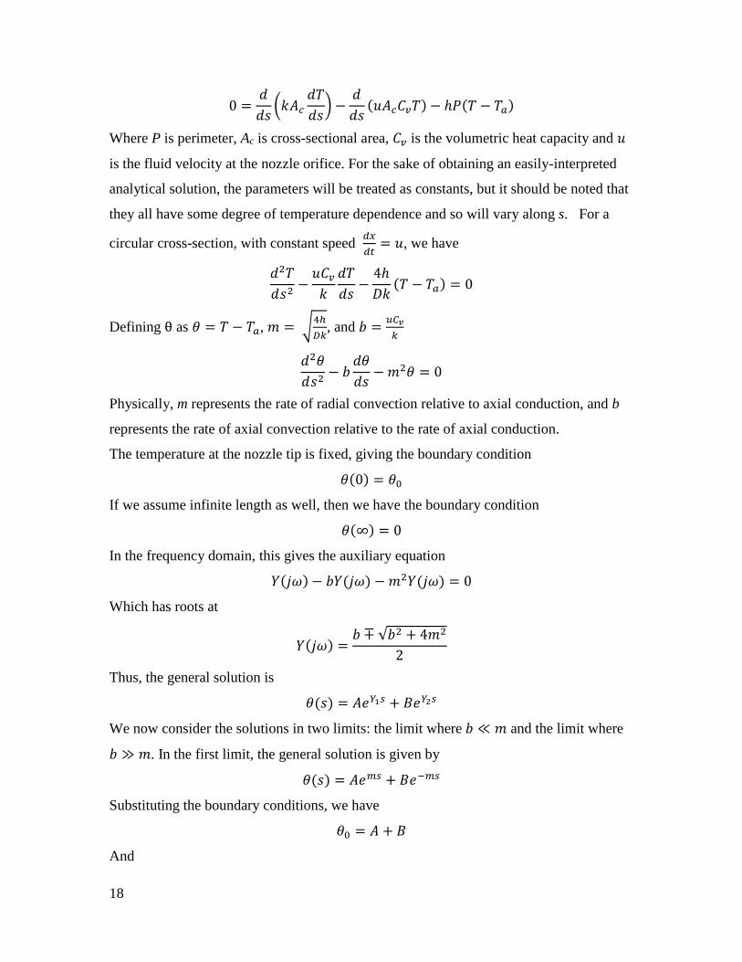
0 =𝑑
𝑑𝑠(𝑘𝐴𝑐
𝑑𝑇
𝑑𝑠) −
𝑑
𝑑𝑠(𝑢𝐴𝑐𝐶𝑣𝑇) − ℎ𝑃(𝑇 − 𝑇𝑎)
Where P is perimeter, Ac is cross-sectional area, 𝐶𝑣 is the volumetric heat capacity and 𝑢
is the fluid velocity at the nozzle orifice. For the sake of obtaining an easily-interpreted
analytical solution, the parameters will be treated as constants, but it should be noted that
they all have some degree of temperature dependence and so will vary along s. For a
circular cross-section, with constant speed 𝑑𝑥
𝑑𝑡= 𝑢, we have
𝑑2𝑇
𝑑𝑠2−𝑢𝐶𝑣𝑘
𝑑𝑇
𝑑𝑠−4ℎ
𝐷𝑘(𝑇 − 𝑇𝑎) = 0
Defining θ as 𝜃 = 𝑇 − 𝑇𝑎, 𝑚 = √4ℎ
𝐷𝑘, and 𝑏 =
𝑢𝐶𝑣
𝑘
𝑑2𝜃
𝑑𝑠2− 𝑏
𝑑𝜃
𝑑𝑠− 𝑚2𝜃 = 0
Physically, m represents the rate of radial convection relative to axial conduction, and b
represents the rate of axial convection relative to the rate of axial conduction.
The temperature at the nozzle tip is fixed, giving the boundary condition
𝜃(0) = 𝜃0
If we assume infinite length as well, then we have the boundary condition
𝜃(∞) = 0
In the frequency domain, this gives the auxiliary equation
𝑌(𝑗𝜔) − 𝑏𝑌(𝑗𝜔) − 𝑚2𝑌(𝑗𝜔) = 0
Which has roots at
𝑌(𝑗𝜔) =𝑏 ∓ √𝑏2 + 4𝑚2
2
Thus, the general solution is
𝜃(𝑠) = 𝐴𝑒𝑌1𝑠 + 𝐵𝑒𝑌2𝑠
We now consider the solutions in two limits: the limit where 𝑏 ≪ 𝑚 and the limit where
𝑏 ≫ 𝑚. In the first limit, the general solution is given by
𝜃(𝑠) = 𝐴𝑒𝑚𝑠 + 𝐵𝑒−𝑚𝑠
Substituting the boundary conditions, we have
𝜃0 = 𝐴 + 𝐵
And

19
lim𝑠→∞
𝐴𝑒𝑚𝑠 + 𝐵𝑒−𝑚𝑠 = 0
This gives
𝜃(𝑠) = 𝜃0𝑒−𝑚2𝑠
𝑠0 = (1
𝑚) ln
𝜃𝑔
𝜃0
𝑠0 = (√𝐷𝑘
ℎ) ln
𝜃𝑔
𝜃0
Physically, this represents the molten length of the filament in the limit of zero
convective heat transfer – in other words, when there is no flow. As expected, this is
identical to the steady-state distribution in a pin fin as given above.
In the limit where 𝑏 ≫ 𝑚, we have
𝜃(𝑠) = 𝐴𝑒(0)𝑠 + 𝐵𝑒𝑏𝑠
In this limit it is impossible to satisfy the boundary condition at infinity. In order to
satisfy the boundary condition at infinity, one root must be positive. We therefore have
𝜃(𝑠) = 𝜃0𝑒−(−𝑏+√𝑏2+4𝑚2
2)𝑠
Where m must be greater than zero. Solving for s such that 𝜃(𝑠) = 𝜃𝑔, the glass transition
temperature, we have
𝑠0 = (2
√𝑏2 + 4𝑚2 − 𝑏) ln
𝜃𝑔
𝜃0
𝑠0 =
(
2
𝑏 (√(1 + (2𝑚𝑏)2
− 1))
ln(
𝑇0 − 𝑇𝑎𝑇𝑔 − 𝑇𝑎
)
The effect of increasing 𝑏 =𝑆𝐶𝑣
𝑘 can be inferred by taking the partial derivative with
respect to this quantity:
𝜕𝑠0𝜕𝑏
=
2 ln (𝑇0 − 𝑇𝑎𝑇𝑔 − 𝑇𝑎
)
√𝑏2 + 4𝑚2(√𝑏2 + 4𝑚2 − 𝑏)

20
This quantity is always positive, indicating that increasing the nozzle speed or the heat
capacity of the material relative to its thermal conductivity will increase the error in the
position of the beam axis.
The effect of increasing 𝑚 = √4ℎ
𝐷𝑘 can be tested in the same way:
𝜕𝑠0𝜕𝑚
= −
2𝑚 ln (𝑇0 − 𝑇𝑎𝑇𝑔 − 𝑇𝑎
)
√𝑏2 + 4𝑚2(√𝑏2 + 4𝑚2 − 𝑏)2
This quantity is always negative, indicating that increasing the convection coefficient
relative to the diameter or thermal conductivity will increase the error in the position of
the beam axis.
The temperature profiles for the parameters given above are shown in Figure 8 for beams
of 100 μm and 1 mm in diameter. The distance at which the beam reaches its glass
transition is an upper bound on the error between the nozzle path and the beam axis. It is
obvious that error can be minimized simply by extruding beams at a slower speed. This is
acceptable for relatively small designs, but for designs comprising thousands of beams,
there is some value to reducing the print time by maximizing the feedrate. This can be
done by increasing h, decreasing 𝑇𝑎, or decreasing 𝑇0.

21
Figure 8 - Simulated beam temperature profiles.
Cv = 4 × 10⁶ J/(m3K), h = 36 W/(m2K) (1 mm beam), 150 W/(m2K) (100 𝛍𝐦 beam), k = 0.25 W/(m*K)

22
It is possible to increase h by adding a cooling fan, and h may be increased and 𝑇𝑎
decreased by refrigerating the printer itself. Neither of these options were seriously
attempted, but they might prove worthwhile if there is a pressing need for very high
throughput freeform 3D printing. Though 𝑇0, the extrusion temperature, is already a free
parameter, it cannot be decreased below 𝑇𝑔, because the material no longer flows below
𝑇𝑔. Additionally, the nozzle must transfer sufficient heat to the joint to fuse the filament,
and this requires a minimum difference between 𝑇𝑔 and 𝑇0. Error can also be decreased
by choosing or designing a material with a low 𝐶𝑣 or a high 𝑇𝑔 relative to 𝑇𝑎. This is
essentially the approach taken here, where isomalt is selected due to its high 𝑇𝑔 relative to
the other sugar alcohols.
Flow Model
Contributing Forces The foregoing analysis does not consider the shape of the beam. The distance at which
the beam reaches its glass transition temperature according to the 1D model is an upper
bound on y(s). In fact, the error for thin beams, on the order of 100 μm, is observed to be
much less than this bound. This is because the shape of the curve is dependent not only
on the length of the molten region, but on the relative strength of gravitational force,
viscous force, and surface tension. We begin with a free body diagram of a beam
extruded from a nozzle that is oriented down and translating left to right, shown in Figure
9. As for the heat transfer model, let s be the vector coinciding with the beam axis. At
any point in the beam, there will be a force parallel to s, T(s), a force perpendicular to s,
N(s), and a moment, M(s). The contributing forces for T(s), N(s), and M(s) are due to
surface tension, viscous force, pressure, and gravity. We begin by considering the relative
importance of each of these forces, beginning with surface tension. For a filament of
diameter D, the axial force due to surface tension is simply
𝑇𝑠 = 𝜋𝐷𝛾
The surface tension of glycerol, 6.3 mN/m, can reasonably be expected to be within an
order of magnitude of the surface tension of molten isomalt. Surface tension also
decreases with temperature, but, for sugar alcohols, this decrease is relatively small. The
temperature dependence of surface tension can be modeled as50

23
𝛾 = (𝜌
𝑀)23⁄
(𝑇𝑐 − 𝑇)
Where 𝜌 is the density, M the molar mass, and 𝑇𝑐 the critical temperature. The critical
temperature of glycerol is 850° K. Thus, the difference in surface tension between
extrusion temperatures (less than 400° K) and room temperature (290° K) would be
expected to be about 25%.
Gravitational force is easily computed using the density of amorphous isomalt, measured
using liquid displacement as 1.5 g/mL. Viscous forces can be estimated using the flow
and feed rates as well as the viscosity of isomalt at different temperatures and water
contents provided by the manufacturer. However, the water content of isomalt processed
according to the protocol in chapter 3 was measured by the manufacturer to be 0.13%,
well below the value typically achieved in processing for pharmaceutical formulations.
Figure 9- Free body diagram for a translating nozzle

24
Because there is no existing data for the viscosity of isomalt with this water content, and
because the temperature at the nozzle tip is not known exactly, an experiment was carried
out to estimate the viscosity of isomalt at typical processing parameters. The lower melt
zone on the extruder, corresponding to the wide section of the nozzle, was set to 130°C.
Isomalt was processed as described in chapter 3 and extruded at several pressures through
a nozzle with a 110 μm inner diameter.
For laminar flow through a tapered nozzle, the viscosity can be estimated using the
lubrication approximation.
𝜇 =𝜋𝑃𝐷4
128𝑄𝐿(
3𝜆3
1 + 𝜆 + 𝜆2)
Where
𝜆 =𝐷0𝐷𝐿
In this case 𝐷0, the diameter at the nozzle inlet, is 4.5 mm, and 𝐷𝐿, the diameter at the
nozzle outlet, is 0.11 mm. L is 9 mm. Using these values and the slope of the pressure-
flowrate graph, the dynamic viscosity is estimated to be 8×10⁶ centpoise. Because the
Figure 10- Isomalt flow rate as a function of pressure

25
temperature is much higher at the nozzle inlet than the nozzle outlet due to the inlet being
closer to the heat source, this is a lower bound on the viscosity at the nozzle outlet.
Given an estimate for the viscosity and surface tension, it is possible to determine the
relative importance of inertial, viscous, gravitational, and surface forces. The associated
non-dimensional numbers are summarized in Table 2.
Table 2 - Dimensionless Numbers For Melt-Extruded Isomalt
𝜇 (cP) 10 7
L (μm) 10 3 10 2
u (mm/s) 1
𝜎(mN/m) 63
𝜌(mg/mL) 1.5
Reynolds Number inertial force
viscous force 𝑅𝑒 =
𝜌𝑢𝐿
𝜇 1.5 × 10 -8 1.5 × 10 -7
Bond Number gravitational force
surface tension 𝐵𝑜 =
𝜌𝑔𝐿2
𝜎 9.3 × 10 -3 9.3 × 10 -1
Capillary Number viscous force
surface tension 𝐶𝑎 =
𝜇𝑢
𝜎 1.6 × 10 2
Galileo Number gravitational force
viscous force 𝐺𝑎 =
𝑔𝐿3𝜌2
𝜇2 1.5 × 10 -10 1.5 × 10 -7
This analysis indicates that viscous forces are much stronger than the other forces
considered. Surprisingly, gravity is dominated not only by viscosity, but by surface
tension as well. This suggests that the vertical error between the nozzle orifice path and
the extruded beam axis is not due to sagging, but rather is a consequence of the nozzle
orifice pointing down. One would then predict that changing the nozzle orientation
would result in the same error perpendicular to the nozzle orifice.
Force due to change in momentum The fluid exiting the nozzle has an initial momentum in both the x and y directions.
However, at low speeds, it can be shown that force required to dissipate this momentum

26
is negligible compared to the viscous force associated with expanding or contracting the
beam axially. This can be inferred from the low value of the Reynold’s number, and
confirmed by the more rigorous analysis given here. A fluid element exiting the nozzle
has an instantaneous x-velocity equal to the nozzle speed. It loses its momentum in the x
direction due to viscous coupling with the portion of the beam that has already been
extruded. The momentum 𝑝 of a differential mass extruded over differential time dt is
given by
𝑑𝑝 = 𝑢𝑄𝑚𝑑𝑡
Where 𝑄𝑚 is the mass flow rate and 𝑢 is the feedrate. Force is simply the time derivative
of momentum. For translation in the x direction,
𝐹𝑥 =𝑑𝑝𝑥𝑑𝑡
= 𝑢𝑄𝑚
Essentially, because the nozzle does not pull the entire beam with it, the rate at which x
momentum is added must be equal to the rate at which it is dissipated through shear. The
force is thus exactly the time derivative of the added momentum, 𝑢Qm. Substituting
diameter for flow,
𝐹𝑥 = 𝑢𝑥𝑄𝑚 = 𝑢 (𝜋𝜌𝑢𝐷𝑏
2
4) =
𝜋𝜌
4(𝑢𝐷𝑏)
2
For feedrates on the order of 10-6 m/s, diameters on the order of 10-4 m/s, and density on
the order of 103 kg/m3, the shear force is on the order of 10-17 N. For comparison, the
volume of isomalt weighing 10-17 N is on the order of 10 picoliters; a 100 micron
diameter beam, 100 microns long, would weigh about this much. This is only the force
required to decelerate each fluid element, not the force associated with viscous stretching,
compressing, or bending the fluid element. The small magnitude of this force suggests
that the latter effects are dominant.
In the y direction, the bulk flow rate is the same, but the velocity is scaled by the ratio of
the nozzle diameter and beam diameter. Thus the expression for the rate at which
downward momentum is added by the nozzle is
𝐹𝑦 = 𝑢𝑦𝑄𝑚 =𝜋𝜌
4(𝑢𝐷𝑏)
2 (𝐷𝑏𝐷𝑛)2

27
Though larger than the rate of momentum addition in the x direction by a factor of (Db
Dn)2
,
this is still on the order of 10-16 N for typical operating conditions, which is much smaller
than gravity. Nonetheless, when the diameter of the nozzle exceeds that of the beam,
considerable deflection is apparent. Thus, we infer that the dominant forces are those
associated with deformation of the beam, discussed next.
Forces due to extensional or compressive flow Within the molten portion of the beam, fluid motion can be described by the Navier-
Stokes equation for incompressible flow.
Figure 11 - Physical meaning of terms in the equation for incompressible flow
Where 𝑢 is the velocity, 𝜈 the kinematic viscosity, and h the sum of the body forces or
head. Head in this case is due to extrusion pressure and gravity. If the direction of nozzle
motion is straight up, perpendicular to the nozzle orifice, then the flow is axisymmetric.
Head loss occurs due entirely to radial flow. If the beam diameter exactly matches the
nozzle diameter, then there is no radial flow, and N(0), M(0), and T(0) are all 0. If the
motion is in any other direction, the molten portion of the beam must bend. In this case
there is flow across the neutral axis of the beam. The viscous resistance to bending and
compression or extension is analogous to the elastic resistance, as shown in Table 3.
In practice, the end of the beam will be fixed to the substrate or to another beam, so that
there is a boundary condition for y(s). As the nozzle moves in a straight line away from
this joint and s approaches infinity, the flow reaches steady-state in the reference frame of
the nozzle. In this case the time-dependent term can be neglected, and the forces are
related exclusively to viscous compression, extension, and bending
𝜕𝑢
𝜕𝑡+ (𝑢 ∙ ∇)𝑢 − 𝜈∇2𝑢 = −∇h
Convective acceleration
Momentum diffusion
Body forces Time-dependent
acceleration
28
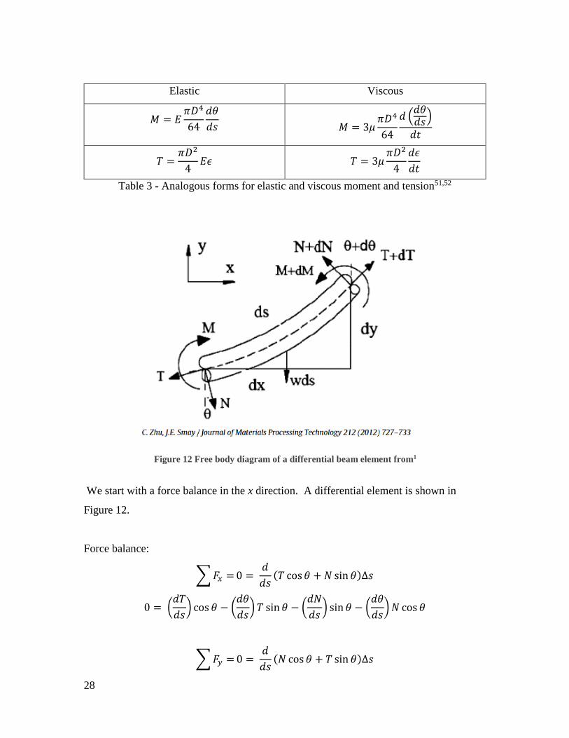
Table 3 - Analogous forms for elastic and viscous moment and tension51,52
We start with a force balance in the x direction. A differential element is shown in
Figure 12.
Force balance:
∑𝐹𝑥 =0 = 𝑑
𝑑𝑠(𝑇 cos 𝜃 + 𝑁 sin 𝜃)Δ𝑠
0 = (𝑑𝑇
𝑑𝑠) cos 𝜃 − (
𝑑𝜃
𝑑𝑠) 𝑇 sin 𝜃 − (
𝑑𝑁
𝑑𝑠) sin 𝜃 − (
𝑑𝜃
𝑑𝑠)𝑁 cos 𝜃
∑𝐹𝑦 =0 = 𝑑
𝑑𝑠(𝑁 cos 𝜃 + 𝑇 sin 𝜃)Δ𝑠
Elastic Viscous
𝑀 = 𝐸𝜋𝐷4
64
𝑑𝜃
𝑑𝑠
𝑀 = 3𝜇𝜋𝐷4
64
𝑑 (𝑑𝜃𝑑𝑠)
𝑑𝑡
𝑇 =𝜋𝐷2
4𝐸𝜖 𝑇 = 3𝜇
𝜋𝐷2
4
𝑑𝜖
𝑑𝑡
Figure 12 Free body diagram of a differential beam element from1
29
0 = (𝑑𝑁
𝑑𝑠) cos 𝜃 − (
𝑑𝜃
𝑑𝑠)𝑁 sin 𝜃 + (
𝑑𝑇
𝑑𝑠) sin 𝜃 + (
𝑑𝜃
𝑑𝑠) 𝑇 cos 𝜃
Incompressibility condition:
𝑉𝐷2 = 𝑐𝑜𝑛𝑠𝑡𝑎𝑛𝑡
𝜕(𝑉𝐷2)
𝜕𝑠= 0
𝐷2𝜕𝑉
𝜕𝑠+ 2𝐷𝑉
𝜕𝐷
𝜕𝑠= 0
𝐷𝜕𝑉
𝜕𝑠+ 2𝑉
𝜕𝐷
𝜕𝑠= 0
Tension/compression relation:
𝑇 = 𝜂𝜋𝐷2
4
𝜕𝑉
𝜕𝑠
Shear-moment relation:
𝑀 = 𝑉𝜂𝜋𝐷4
64
𝜕2𝜃
𝜕𝑠2
𝑁 = −𝑑𝑀
𝑑𝑠=−𝜋
64(𝑉𝜂𝐷4
𝜕3𝜃
𝜕𝑠3+ 4𝑉𝜂𝐷3
𝜕2𝜃
𝜕𝑠2+ 𝑉
𝜕𝜂
𝜕𝑠𝐷4𝜕2𝜃
𝜕𝑠2+𝜕𝑉
𝜕𝑠𝜂𝐷4
𝜕2𝜃
𝜕𝑠2)
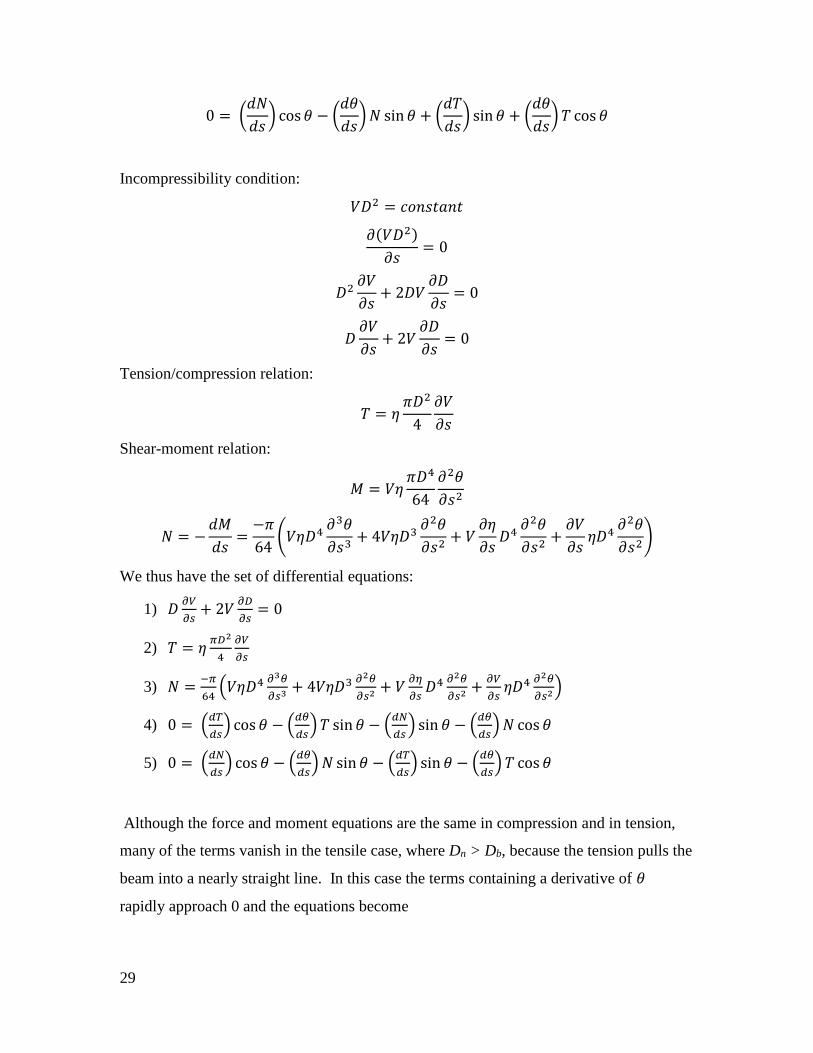
We thus have the set of differential equations:
1) 𝐷𝜕𝑉
𝜕𝑠+ 2𝑉
𝜕𝐷
𝜕𝑠= 0
2) 𝑇 = 𝜂𝜋𝐷2
4
𝜕𝑉
𝜕𝑠
3) 𝑁 =−𝜋
64(𝑉𝜂𝐷4
𝜕3𝜃
𝜕𝑠3+ 4𝑉𝜂𝐷3
𝜕2𝜃
𝜕𝑠2+ 𝑉
𝜕𝜂
𝜕𝑠𝐷4
𝜕2𝜃
𝜕𝑠2+𝜕𝑉
𝜕𝑠𝜂𝐷4
𝜕2𝜃
𝜕𝑠2)
4) 0 = (𝑑𝑇
𝑑𝑠) cos 𝜃 − (
𝑑𝜃
𝑑𝑠)𝑇 sin 𝜃 − (
𝑑𝑁
𝑑𝑠) sin 𝜃 − (
𝑑𝜃
𝑑𝑠)𝑁 cos 𝜃
5) 0 = (𝑑𝑁
𝑑𝑠) cos 𝜃 − (
𝑑𝜃
𝑑𝑠)𝑁 sin 𝜃 − (
𝑑𝑇
𝑑𝑠) sin 𝜃 − (
𝑑𝜃
𝑑𝑠) 𝑇 cos 𝜃
Although the force and moment equations are the same in compression and in tension,
many of the terms vanish in the tensile case, where Dn > Db, because the tension pulls the
beam into a nearly straight line. In this case the terms containing a derivative of 𝜃
rapidly approach 0 and the equations become

30
1) 𝐷𝜕𝑉
𝜕𝑠+ 2𝑉
𝜕𝐷
𝜕𝑠= 0
2) 𝑇 = 𝜂𝜋𝐷2
4
𝜕𝑉
𝜕𝑠
3) 𝑁 = 0
4) 0 = (𝑑𝑇
𝑑𝑠) cos 𝜃
5) 0 = − (𝑑𝑇
𝑑𝑠) sin 𝜃
It follows from either equation 4 or equation 5 in this case that 𝑑𝑇
𝑑𝑠= 0 and that the
tension is uniform throughout the entire beam. This case can be described by existing
models for fiber drawing.52
In the compressive case, at the nozzle orifice (s = 0), the beam diameter is equal to the
nozzle diameter. Using the frame of reference of the nozzle, the initial velocity in the x
direction is zero. Because the beam cannot rotate instantaneously, the axis at s = 0 must
be perpendicular to the nozzle orifice. This gives the boundary conditions
{𝜃 = 90, 𝐷 = 𝐷𝑛, 𝑉 = 0 𝑠 = 0, }
{𝜃 = 0 , 𝐷 = 𝐷𝑏 𝑉 = 𝑢, s0 = ∞}
We have 5 equations relating D, V, T, N and θ to the parameter s. 𝜂 is a function of
temperature. Given 𝜂(𝑠) these equations could be solved. However, even without 𝜂(𝑠),
the heat transfer model and equation 2 can be used to determine a lower bound on the
force required to deform the beam. When the beam diameter is Db and the nozzle
diameter is Dn, and the diameter change takes place over some distance 𝑠0, the lowest
axial velocity gradient occurs when the rate of speed reduction with respect to axial
distance is uniform over 𝑠0. If mass is conserved and the nozzle translation speed is 𝑉,
then the translation speed at 𝑠0, is simply 𝑉0 (𝐷𝑛
𝐷𝑏)2
. Thus,
𝜕𝑉
𝜕𝑠>𝑉0𝑠0(1 − (
𝐷𝑏𝐷𝑛)2
)
So that the force at the nozzle orifice is bounded below by

31
F >3𝜋
4
𝜂𝑉0𝑠0(𝐷𝑛
2 − 𝐷𝑏2)
The length 𝑠0 is bounded by the distance traveled before the material reaches its glass
transition temperature. If s0 is on the order of mm, then F is relatively large. For
example, for a 200 μm beam extruded through a 100 μm nozzle, the axial force is greater
than 10-5 N. Thus, the force due to the extrusion pressure will be many orders of
magnitude greater than the force due to shear even for small differences between the
beam and nozzle diameters. Shear can be neglected, and any deformation can be
accurately modeled using a load perpendicular to the nozzle orifice.
It is also useful to consider the limiting case where the nozzle is not translating. In this
case (u = 0), the beam will eventually expand so that its diameter is much greater than the
nozzle diameter. This case is not accurately represented by the 1-D heat transfer model
derived previously. When the diameter of the beam is large relative to its length, the
lumped capacitance approximation is invalid, and the temperature at the beam surface is
not equal to the nozzle temperature. The temperature at the beam surface will approach
room temperature, and will become stiff. The flow will then approach zero and the force
on the beam will simply be the product of the extrusion pressure and the nozzle cross-
sectional area. At typical pressures, this is on the order of mN. Again, the potential
magnitude of this force indicates that viscous resistance to radial flow needs to be
considered.

32
Experimental Characterization of Beam Shape and Force
Error The diameter and vertical error of horizontal beams were measured experimentally from
a series of bright field images as shown in Figure 13. The error y in this case is the
distance between the nozzle orifice and the top of the extruded beam. Briefly, isomalt
was prepared as described in chapter 2 and extruded through a 110 μm diameter nozzle.
The NI Vision package for LabVIEW was used to determine diameters with the aid of
automated edge detection. It was found that, at each feedrate used, the beam area (and
thus the flow rate) scaled linearly with the applied pressure.
D
y
Figure 13 - Test case for beam axis error

33
Figure 14 - Diameter and Flow Rate as a Function of Pressure and Feedrate

34
It is useful to scale the feedrate, flow rate, and diameter by the nozzle diameter, Dn as
follows.
Feedrate, �̅� =𝑢
𝐷𝑛
Diameter, �̅� =𝐷
𝐷𝑛
Flow rate, �̅� =𝑄
𝐷𝑛3
Error, �̅� =𝑦
𝐷𝑛
It is clear from Figure 14 that there is a reduction in flow at lower feedrates. However, it
appears that the flow is still linear with pressure at each feedrate. Plotting the ratio of
pressure to �̅�2 against feedrate in Figure 15, we obtain a nearly straight line. From
Figure 15,
Figure 15 - Flow Resistance as a Function of Feedrate
𝑃
�̅�2= 𝑅 ∗ �̅�

35
𝑃 = 𝑅�̅� = 𝑅�̅��̅�2
R is found to be 12 PSI×s-1. It is important to note, however, that R is the sum of the
nozzle resistance Rn and the viscous resistance associated with expanding the beam from
the nozzle diameter to its final diameter, Rv. It is clear from the plot of pressure vs. flow
that for this experiment, Rv is small for feedrates greater than 200 μm/s. If the pressure
drop due to viscous losses outside the nozzle is negligible compared to the pressure drop
across the nozzle, then Rv is small relative to Rn and the nozzle resistance alone
determines the flow. This appears to be the case for feedrates greater than 200 μm/s.
At any given feedrate, the heat transfer model predicts that larger diameter filaments will
have a greater error �̅�. It was found that for each feedrate, the error scaled linearly with
the area of the filament. The slope relating �̅� and �̅�2 can in turn be used to find a
correlation between �̅� and �̅�. These quantities are plotted against each other in Figure 16.
It is found that, for �̅� > 1 the relationship between error, diameter, and feedrate can be
modeled as
�̅� = 𝐶(�̅� − 1)�̅�
Solving for �̅�,
�̅� = (�̅�
𝐶�̅�+ 1)
In this case, C = 0.11 seconds. This relation can be used to find the maximum permissible
u for any desired D and y. First u is found from the above relation. Then, the known
nozzle resistance is used to find P using
𝑃 = 𝑅�̅��̅�2
Substituting,
𝑃 = 𝑅 (�̅�
𝐶+ �̅�)
𝑃 = 110�̅� + 12�̅�
For any given diameter and tolerance on the error, these relations will give the
appropriate combination of pressure and feedrate.

36
Figure 16 - Error as a Function of Diameter and Feedrate

37
Force When the diameter of the beam is not matched to that of the nozzle, the beam must
stretch or compress. As noted earlier, the force associated with this deformation is
related to the rate of change of speed and the viscosity by
F =ηπ𝐷2
4
∂Vs∂s
Where η is the Trouton viscosity, thrice the kinematic viscosity. The force can be tensile
or compressive. However, we shall consider only compressive forces. The reason for this
is that, to avoid build-up of material on the nozzle, it is preferable to use as fine a tip as
possible. A wider nozzle, when placed at an existing joint, is likely to melt beams
incident at that joint and pull the material with it as it translates. Thus, it is almost always
preferable to print with a nozzle that has diameter less than or equal to the diameter of the
thinnest desired beam.
The force exerted by the nozzle can be measured optically as shown in Figure 17 by
measuring the deflection of a thin, cantilevered beam. Given the material properties, the
force and backpressure at the nozzle orifice can be calculated as follows. For a simply
cantilevered beam with a circular cross-section, the deflection due to a point load at the
beam endpoint is given by
𝛿 =64𝐹𝐿3
3𝜋𝐷4𝐸
Where F is the force and E is the elastic modulus. Solving for the backpressure,
𝑃𝑛 =3𝐷4𝐸𝛿
16𝐷𝑛2𝐿3
Using L = 5 mm, D = 160 μm, Dn = 110 μm, 𝛿 = 250 μm, and E = 2.6 GPa53, the
backpressure at the nozzle orifice is about 8 PSI. This is small compared to the extrusion
pressure, which is measured within the extruder barrel. However, this pressure is not
necessarily small compared to the pressure immediately inside the nozzle. At lower
feedrates, the pressure drop due to radial flow is significant and causes the flow rate to
decrease.

38
𝛿
160 μm
5 mm
Figure 17 - Test case for beam deflection due to extrusion back-presure. Rightmost vertical beam
printed at 500 PSI and 0.1 mm/s.
Figure 18 - Deflection as a function of flow rate

39
This can be seen in the data set below, which corresponds to the test case given above.
Diameter and deflection were measured at 100, 200, and 400 μm/s, at pressures of 100,
200, 300, 400, 500, and 600 PSI.
The deflection is seen to increase for slower feedrates, and to increase monotonically
with flowrate at each given feedrate. However, the slope decreases with flow rate,
indicating that the viscous resistance to radial flow decreases at larger diameters. This
may occur because, at higher flow rates, the temperature at any point along s is greater.
The higher temperature reduces the viscosity, decreasing the viscous resistance to radial
expansion.
Because freeform assembly designs specify diameters, not flow rates, it is helpful to
establish a direct correlation between the force exerted by the nozzle and the diameter.
Conveniently, the force appears to scale linearly with the diameter. Assuming that elastic
beam theory applies, we can convert deflection to units of force as above:
Figure 19 Flow rate as a function of pressure, deflection test case

40
This relationship is very important. It indicates that the force exerted by printing any
beam is dependent only on beam diameter.
Figure 20- Deflection and load as a function of diameter

41
Orientation Natural convection will depend on the beam orientation, which will affect the
temperature profile and thus the viscosity profile. In principle, this could mean that, at a
given feedrate and pressure, the flow rate would change with orientation. However, for
the parameter range of interest, the pressure drop associated with expanding the fluid
beam is, much smaller than the pressure drop due to the nozzle resistance. Thus the
effective resistance to flow should be nearly constant with beam orientation, unless a
change in orientation changes the heat transfer rate so much that it affects the temperature
of the material inside the nozzle tip. This can easily be verified by experiment. In order
to test the effect of nozzle motion direction on the beam diameter, horizontal and vertical
beams were printed at the same pressures and feedrates and measured from a bright-field
image as shown in Figure 21. The NI Vision package for LabVIEW was used to
determine diameters and errors with the aid of automated edge detection. As shown in
Figure 21, the diameters at a given pressure and feedrate are identical within 2 pixels
Dh
Dv
Figure 21 -Vertical vs. and horizontal diameter test case

42
irrespective of feedrate and orientation. The independence of diameter and orientation
suggests that the temperature profile and therefore the viscosity profile is not affected by
the orientation of the beam, at least between 0° and 90°.
Figure 22 - Effect of beam orientation on diameter. Dn is the diameter of the nozzle, 110 μm

43
Chapter 4: Freeform Assembly Planning
A great deal of this section has been submitted nearly verbatim for publication. I would
like to acknowledge my co-author Greg Hurst for fruitful discussions and implementing
the planning algorithm in efficient code.
AND/OR Constraints
The process of assembly can be thought of as iteratively combining subassemblies into
larger subassemblies until the final assembly is complete. In the case of freeform
assembly, only one beam is added at each step, and each subassembly step consists of
combining two subassemblies: one comprising a single beam, the other comprising all
beams already printed. In this case the assembly process is analogous to task sequencing,
where the tasks correspond to the printing of individual beams. A state is defined as the
set of tasks that have not yet been completed. Thus the number of possible task
sequences is at least as large as the number of possible states.
Relationships between tasks as well as between states can be defined using constraints
known as AND/OR constraints, and graphically represented using AND/OR graphs. An
AND constraint signifies that a task j may be completed only after every other task in
some set I has been completed. For each task i in set I, we say that say task i must
precede j, that j must succeed i, or that i ≻ j. To indicate that i can precede j, we use the
notation i ≽ j. An OR constraint signifies that a task j can be completed after any task in
another set I has been completed. In some cases tasks will have complex combinations of
AND constraints and OR constraints. Consider the following example:
((A ≻ D) ∧ (B ≻ D)) ∨ (C ≻ D)
((A ∧ B) ∨ C) ≻ D

44
Figure 23 - AND/OR Precedence Graph
We have two conditions that allow us to complete task D: complete C, or complete both
A and B. In order to completely represent the set of task constraints, we must introduce
an optional task, or place, A ∧ B. The terminology here is borrowed from a representation
of assembly process constraints using petri nets.54 This representation is essentially
equivalent to the AND/OR graph representation55, and we shall adopt the AND/OR graph
convention here.
AND/OR constraints can be represented by a directed bipartite graph, in which every
edge exiting an AND node enters an OR node, and every edge exiting an OR node enters
an AND node. In this case the AND nodes represent tasks or places, and the OR nodes
represent waiting conditions.56 AND nodes can be visited only after every one of their
source nodes has been visited. OR nodes may be visited after any one of their source
nodes is visited. Below, we show the AND/OR graph for the example given above.
C
A
B
OR 𝐴 ∧ 𝐵 D

45
A common problem is determining an optimal sequence for the tasks. In order for an
optimal sequence to exist a feasible sequence must exist such that no precedence
constraint is violated. For a graph containing only AND nodes, feasibility is assured
provided the graph is ayclic. This implies that there is no pair of tasks such that i ≻ j and
j ≻ i. If an OR node has only one incoming edge, it is equivalent to an AND node.
Therefore, we can decompose an AND/OR graph into the set of AND graphs created by
choosing a single incoming edge for each OR node. If any of these AND graphs is
acyclic, there exists a feasible sequence for the AND/OR graph. An example of this OR
decomposition is shown in Figure 24.
In this example there is no combination of OR choices that produces an acyclic graph.
Thus, there is no feasible task sequence. Equivalently, one may identify all the cycles in
an AND/OR graph. If a cycle contains only AND nodes, there is no feasible sequence.
Each unique cycle containing an OR node corresponds to a unique realization of the OR
constraints. Therefore if the number of cycles is less than the possible combinations of
OR choices, there exists a feasible sequence. It is possible to determine a feasible
sequence for a complete set of AND/OR precedence constraints in linear time.56
However, for complex assemblies subject to stability constraints, the complete set of
B
A
C
OR
B
A
C
ORR
B
A
C
OR B
A
C
B
A
C
Figure 24 - AND/OR Decomposition

46
precedence constraints is too large to enumerate. In this case it becomes more useful to
consider the assembly states, which can also be represented using AND/OR graphs.57,58
AND/OR graphs track only the state of an assembly – that is, the set of parts that have
been placed in their final configuration with respect to one another. Typically, when
generating an assembly graph, one starts with the fully assembled state and iteratively
decomposes the assembly into 2 or more subassemblies. When removing only 1 part at a
time, the process of removing a part can be considered a task, subject to set of partial
ordering constraints as defined above. Thus a state is equivalent to the set of all tasks not
yet performed.
Figure 25 shows an example of an assembly tree and the corresponding task precedence
graph. Parts A, B, and C are blocks to be assembled as shown, subject to gravitational
force.

47
B C
A
B
A
B C
B C
C
A
B
OR
A
A B
OR
OR
A C
C B
C
B
OR
A
A C C
Figure 25 Disassembly tree and precedence graph for a block tower

48
In Figure 25, the state containing parts A and C only is unstable. Block A will fall over
unless it is supported in the middle by block B. Removing block B first is equivalent to
drawing an edge from B to A and C in the precedence graph; this creates a cycle,
indicating that there is no feasible sequence if B is removed first. We shall define an
unstable state as a state created by performing a task that is a member of a cycle.
There will be some assembly states which, while not unstable, cannot actually be
constructed without creating an intermediate unstable state. Consider the example in
Figure 26. We know that the earliest possible state at which A can be removed is the state
at which only its AND predecessors have been removed. If A must precede each of the
remaining tasks, then this look-ahead state is unavoidable and is the only state at which A
can be removed. In the example above, removing C causes the state at which A must be
removed to be unstable. We can therefore infer that A ≻ C.
In some cases, some of the parts in the look-ahead state need not succeed A. However,
we can sometimes determine that there is no subset of these which, if removed, would
stabilize the assembly so that A can be removed. An example is shown in Figure 27
A E
Assembly State Precedence Graph Look-ahead State for A
B C
A
D E D
B C
A
B
A
D E
B
A A E
D
C
Figure 26 - Look-ahead state example 1

49
Figure 27 - Look-ahead state example 2
If there is an additional block, F, next to B, either F or B can be removed before A.
However, the stability criterion in this case is related to the position of B alone, and we
can infer the new precedence constraint A ≻ C based on the look-ahead state without
considering each of its sub-states.
Stability of a given look-ahead state does not imply reachability for that state. A counter-
example is shown in Figure 28. Removing C does not result in an unstable state, but
nonetheless creates a dead end, because there is no sequence in which D and E can be
removed without creating an unstable intermediate state. This dead end cannot be
anticipated solely based on a look-ahead state. This is a problem because, for more
complex examples, it isn’t obvious where the dead-end branch diverged from the
assembly tree. Although in this case there are only 2 possible states between the unstable
state and the first unconstructable state, for more complex assemblies, there can be too
many intermediate sequences to explore exhaustively. It is thus critical that such
unconstructable states be identified immediately. Whether this is possible depends on the
structure of the underlying AND/OR precedence constraints, which are determined by the
physics of the problem.
A E
Assembly State Precedence Graph Look-ahead state for A
B C
A
D E D
B C
A
B
A
D E
B
A A E
D
C
F
F
F
F

50
For example, in the limit as B becomes infinitely thin, the center of gravity of every block
resting on A must lie directly over B. Any configuration of blocks failing this condition
is unconstructable. Under less restrictive conditions, unconstructable states may be
identifiable only by exploring the entirety of the disassembly branch. If all possible
sequences beginning at this state terminate in unstable states, the state is unconstructable.
In the following section, we examine the assembly planning problem for the constraints
specific to freeform assembly.
State-Space Planning
Freeform assemblies can be concisely represented using a graph data structure. We refer
to the nodes of this graph as joints and the edges of this graph as beams. Each joint is
specified by an xyz coordinate. Each beam is specified by a thickness, which may vary
along its length, and a 3D path connecting its two joints. Choosing an order in which to
print the beams can be formulated as an assembly sequencing problem. Here we consider
B C
A
D E
A
D
E
B
A
D E
Assembly State Precedence Graph Look-ahead State
B C
A
B
A
A
D
E
B
A
D
B
A
A
D
E
B
B
Figure 28 - Unreachable look-ahead state

51
assembly sequences that are linear and monotone.59 In a linear assembly, exactly one
part is attached to the rest of the assembly at each step. In a monotone assembly, once
added, no part is ever removed from the assembly. These constraints are appropriate for
freeform 3D printers that print using one nozzle at a time and cannot remove any material
that has already been printed.
The essence of most assembly planning approaches is a search through the assembly state
graph.58 In this graph, each state is either a single part or a set of parts that have been
placed in their final configuration with respect to each other. The graph is initialized with
states corresponding to single parts, and new states are generated from the union of
existing states. An example assembly graph for a freeform printed assembly is shown in
Figure 30.
For assemblies containing a sufficiently large number of parts, generating the entire
assembly state graph is computationally prohibitive. It is only necessary to search the
assembly graph for a path from the completely disassembled state to the completely
assembled state.57 The search may be initiated from either of these states. If starting from
the completely disassembled state, a part added at one step may obstruct the placement of
another part at a later step. Thus a forward search can result in dead-end states from
which the assembly cannot be finished. For this reason, the graph search is typically
begun from the completely assembled state. New states are generated by separating pairs
of subassemblies, generating a disassembly sequence. Reversing the disassembly
sequence gives the forward assembly sequence. Separating a subassembly will never
create a new obstruction for the remaining parts; thus, if collision is the only constraint on
the process, this approach will never create a dead-end state. Under stability constraints,
however, it is possible to generate dead-end states even in the disassembly graph search.
The problem of assembly sequencing under stability constraints has been investigated for
block towers60,61, frame structures62,63, and mechanical assemblies for which stability is a
function of orientation60,64,65. In these planning approaches, the problem of dead ends is
avoided by allowing scaffolding or reorientation. Unstable states are penalized with a

52
scaffolding or reorientation cost, but the planner does not backtrack in search of a
sequence that minimizes this cost. Though freeform assembly is compatible with
scaffolding, the placement and removal of scaffolding introduces additional physical as
well as computational steps. A more elegant approach would identify sequences that
contain no unfinishable or unconstructable states, so that no scaffolding is required. We
prove that, for freeform assembly using a material that stiffens via a reversible glass
transition, this problem is NP-complete. However, for the types of geometries one would
commonly encounter, we show that sequences that are feasible and even optimal under
certain cost functions can be found efficiently. Lastly, we validate our approach by
physically printing large assemblies composed of thousands of beams.
Freeform Process Constraints
Different freeform assembly processes are subject to different subsets of the following
constraints. If beam A must be printed before beam B, we say that A precedes B (𝐴 ≺ 𝐵),
or that B succeeds A (𝐵 ≻ 𝐴).
Directionality: No beam can be printed in such a way that would cause the nozzle to
collide with that beam during printing. For example, for the 3-axis printer considered
here, vertical beams must be printed bottom-to-top. Some beams will be unprintable from
either direction, and any assembly containing such a beam will be unconstructable. If a
beam is directed such that it must be printed starting from joint p, it succeeds at least one
other beam incident to joint p.
Collision: No beam can be printed that would cause the nozzle to collide with a
previously drawn beam. If the volume swept out by the nozzle while printing beam A
intersects any part of beam B, then 𝐴 ≺ 𝐵.
Connection: Each successive beam must start from a joint on the substrate or a joint to
which a previously printed beam is incident. Any beam containing non-grounded joints p
and q must succeed at least one of the other beams incident to joint p or joint q.

53
Cantilever: When stiffening is achieved via cooling below the glass transition
temperature, special consideration must be given to the effect of heating an existing joint.
When fusing a new beam to an existing joint, the heat of the nozzle may cause the joint to
become fluid and unable to sustain a bending moment. (Supplementary video 1). Any
cantilevered beams attached to the joint will pivot due to the moment caused by their own
weight. This introduces a cantilever constraint: new beams cannot be connected to joint p
if any previously printed beam incident to joint p is cantilevered. It may be possible to
limit heat flow to the joint and prevent pivoting – for example, by depositing extra
material at the joint, or by offsetting the nozzle slightly – but we will treat this as an
absolute constraint in order to obtain a highly robust assembly sequence. Any beam
cantilevered about joint p must succeed all other beams incident at p. Note that, unlike
the other constraints, this constraint only applies to some subset of the possible assembly
states.
Figure 29 - Freeform Assembly Constraints

54
All freeform assembly processes are subject to directionality and collision constraints.
Free-standing assemblies are subject to the connection constraint, and assemblies in
which stiffening is achieved by a reversible glass transition are subject to the cantilever
constraint. In the absence of the cantilever constraint, finding a feasible sequence is
analogous to task planning under AND/OR constraints, and can be done in linear time
with respect to the number of beams56. Here we show that the addition of the cantilever
constraint renders the problem NP-complete.
As in traditional assembly planning, our approach will use a state-space search. Though
assembly sequencing is often done by finding a disassembly sequence and reversing it,
we will use a forward search. The first reason for this is that a forward search is more
intuitive. The second reason is that, while a disassembly planner must finish the entire
sequence before the physical printing process can begin, a forward planner can be run
concurrently with a printer, generating the sequence on the fly. For large designs where
sequence generation is computationally intensive, using a forward planner instead of a
backward planner can thus reduce the total assembly time by a factor of up to 2. All of
the arguments made apply to the disassembly problem as well, and an essentially
identical approach could be applied to generate a disassembly sequence.
Computational Complexity
We seek a sequence of beams and a printing direction for each beam that is consistent
with all of the process constraints. Collision, connection, and directionality constraints
between any pair of beams are the same regardless of the sequence of states, but the
cantilever constraint is a function of the assembly state itself, and different cantilever
constraints will be encountered for different sequences. This renders the problem much
more difficult (in fact, NP-complete), because a naive graph search may reach a dead end
state whether the search is initiated from the full state or the empty state. Reaching a
dead end requires backtracking to a previous state to resume the search. In the worst case,
the search will enumerate the entire graph.

55
State G4 in Figure 30 can be immediately identified as a disassembly dead end because
there is a joint supporting 2 cantilevers, resulting in conflicting precedence constraints;
the magenta and blue beams must precede each other due to the cantilever constraint,
which makes it impossible to assemble both of them. Similarly, state G2 can be
immediately identified as an assembly dead end because assembling either the yellow or
Figure 30-Freeform Assembly State Graph.
Because the assembly is monotonic, each new state is the union of an existing state and a single beam.
The single part is not shown in the graph, so each state above is equivalent to an OR node

56
magenta beams would violate the cantilever constraint. However, there can exist states in
which no conflict is immediately identifiable, but which are nonetheless dead ends. An
assembly search may reach a state from which the full assembly is unconstructable, as
occurs in state G1, while a disassembly search may encounter a state that is
unconstructable from the empty state, as occurs in state G3. In order to search the graph
efficiently, one must have a means of avoiding these branches from which the goal state
is unreachable. Determination of a feasible sequence is polynomial time reducible to the
decision problem of state reachability, Reachable(G,H). This function returns true if there
exists a sequence of beams that can be successively added to assembly state G to create
assembly state H without violating any process constraints. The reduction can be done as
follows:
Function Sequence(G,H)
G← empty assembly state
H← full assembly state
b← beams
seq← ∅
while length(b)>0 do
for i = 1…length(b) do
if Reachable(G∪b(i), H) then
seq←append(seq, G∪b(i),)
G← G∪b(i),
b←delete(b,i)
break()
if i = length(b) then
return unprintable
return seq
We now prove that state reachability is NP-complete by polynomial time reduction from
circuit satisfiability (circuit-SAT). The circuit-SAT problem asks if, given an arbitrary
Boolean expression, there exists a satisfying assignment to each variable such that the
57
expression evaluates to true. We will show that, for any instance of circuit-SAT, it is
possible to design an assembly such that, if the full assembly state is reachable from the
empty state, then the corresponding instance of circuit-SAT is satisfiable. The logic is as
follows: We design an assembly that can be fully assembled if and only if one particular
circuit “output” beam can be assembled. If the circuit output beam and thus the full
assembly state can be assembled, then Reachable(Empty State, Full State) will return
true. If the output beam cannot be assembled, then the full assembly state is unreachable
as well, and Reachable(Empty State, Full State) will return false. Each variable in the
instance of circuit-SAT represented by this assembly will correspond to a specific beam
in the assembly. If a variable is true, then its corresponding beam must be assembled
before the output beam. If a variable is false, then its corresponding beam must be
assembled after the circuit output beam. If the circuit output beam can be assembled, its
value is true, and there exists a satisfying assignment for the circuit that the assembly
instantiates.
This scheme transforms a set of Boolean constraints between variables into a set of
precedence constraints between beams. In order to represent any instance of circuit-SAT,
we need a method of imposing arbitrary precedence constraints between the variable
beams. This requires introducing additional beams to create “gadgets” and “wires”, as in
classical circuit-SAT proofs. The gadgets will be composed of 1 or 2 gadget input beams,
1 or 2 gadget output beams, and several gadget beams that create certain precedence
relationships between the gadget input and output beams and the circuit output beam. The
wires will be single beams that connect the output of one gadget to the input of another
gadget. The variable beams are thus equivalent to wires that are connected only to the
inputs of a gadget.
Any Boolean operation or logic gate can be represented using either of 2 universal
gadgets, NAND or NOR, and a splitter gadget. The splitter gadget creates two output
wires with the same value as the input wire; this is necessary for this proof because wires
are represented by single beams, which can only connect one gadget input to one gadget
output. We will implement the NOR and splitter logic gates by introducing a set of beams

58
such that, for each state of the gate, there is exactly one state of the gadget that would
enable assembly of the output beam. Before describing the gadgets, we begin with some
preliminary definitions:
Definition 1. A beam path is a path in the sense of graph theory, i.e., a connected acyclic
set of beams.
Definition 2. A joint p is stable there are 2 or more paths from p to a grounded joint that
intersect only at p. A path is stable if all the joints in it are stable.
Definition 3. A joint is grounded if it is on the substrate. Grounded joints are always
stable.
Definition 4 A connected subassembly is a connected component in the sense of graph
theory, where the beams are the graph edges and the joints are the nodes. For each
connected subassembly, there is a path between any 2 joints in that connected
subassembly.
The gadgets are shown in the following pages in a top-down view. If beam A crosses over
beam B, then 𝐴 ≺ 𝐵 in accordance with the collision constraint. Joints are represented by
dots. Green joints are grounded. Wires are represented by white beams, and gadgets are
represented by red, blue, and magenta beams. For both gadgets, there is a loop connected
to a grounded joint. Due to the cantilever constraint, one half (the red or blue path) of the
loop must be assembled and made stable before the other half is assembled. The only way
to stabilize the red or blue path is to assemble the magenta path and connect it to the
circuit output beam. Thus, exactly one path in the loop must be assembled before the
circuit output beam, and the other path in the loop must be assembled after the circuit
output beam. This XOR relationship can be exploited to yield both a splitter and a NOR
gate by designing the gates such that inputs or outputs must precede or follow some
portion of one of the red or blue paths. Note that this state constraint is only possible if
the cantilever constraint applies; without it, only AND/OR precedence relations between
states are possible, and the problem is in P.
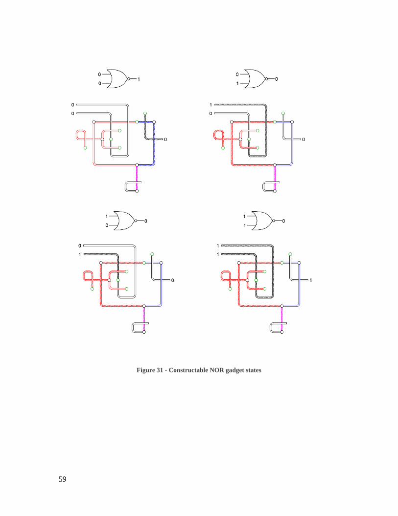
59
Figure 31 - Constructable NOR gadget states

60
Figure 32 - Constructable splitter gadget states
As in the NOR gadget, exactly one of the red or blue paths must precede the output beam, which is
shown in white crossing the magenta beam.
Splitter
NOR
Circuit output beam
Figure 33 –X NOR X Instantiation
The magenta beams are stabilized by the assembly of a beam that is directed out of the end joint of
the output beam. This ensures that the magenta beams cannot be stabilized by connection to each
other. Hatches indicate that a beam is assembled; 0 indicates true, and 1 indicates false

61
In order to connect to the circuit output beam, the magenta gadget beams must cross over
other wire beams, implying a precedence relation. Furthermore, the magenta beams must
sometimes follow some of the input or output beams of the gadget from which they
originate. However, this does not prevent instantiation of an arbitrary circuit. All magenta
beams, but not all wire beams, must be assembled before the circuit output beam if the
assembly is to be constructable. Therefore we must ensure that the magenta beams can be
assembled before any wire beams that they cross, for any state of the circuit. Suppose the
gadgets are arranged on a grid, and the magenta beams are routed to the right of their
respective gadgets and then down to the bottom of the diagram, as shown in figure 3.
The gadget states are assembled column-by-column, starting from the left, and each
column is assembled starting from the top and proceeding down. In this way, the
magenta beams can always be assembled before any wire beams they cross.
Figure 34- Circuit layout
Each box can represent either a splitter or a NOR gate, and so has at most 2 inputs and at most 2
outputs. If the gadgets are assembled top-to-bottom, starting at the leftmost column and proceeding
to the right, then no magenta beam will ever prevent assembly of any wire beam.
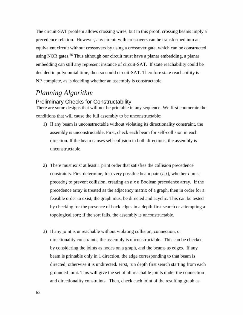
62
The circuit-SAT problem allows crossing wires, but in this proof, crossing beams imply a
precedence relation. However, any circuit with crossovers can be transformed into an
equivalent circuit without crossovers by using a crossover gate, which can be constructed
using NOR gates.66 Thus although our circuit must have a planar embedding, a planar
embedding can still any represent instance of circuit-SAT. If state reachability could be
decided in polynomial time, then so could circuit-SAT. Therefore state reachability is
NP-complete, as is deciding whether an assembly is constructable.
Planning Algorithm
Preliminary Checks for Constructability There are some designs that will not be printable in any sequence. We first enumerate the
conditions that will cause the full assembly to be unconstructable:
1) If any beam is unconstructable without violating its directionality constraint, the
assembly is unconstructable. First, check each beam for self-collision in each
direction. If the beam causes self-collision in both directions, the assembly is
unconstructable.
2) There must exist at least 1 print order that satisfies the collision precedence
constraints. First determine, for every possible beam pair (𝑖, 𝑗), whether i must
precede j to prevent collision, creating an n x n Boolean precedence array. If the
precedence array is treated as the adjacency matrix of a graph, then in order for a
feasible order to exist, the graph must be directed and acyclic. This can be tested
by checking for the presence of back edges in a depth-first search or attempting a
topological sort; if the sort fails, the assembly is unconstructable.
3) If any joint is unreachable without violating collision, connection, or
directionality constraints, the assembly is unconstructable. This can be checked
by considering the joints as nodes on a graph, and the beams as edges. If any
beam is printable only in 1 direction, the edge corresponding to that beam is
directed; otherwise it is undirected. First, run depth first search starting from each
grounded joint. This will give the set of all reachable joints under the connection
and directionality constraints. Then, check each joint of the resulting graph as

63
follows: if every beam directed out of the joint must precede every edge directed
into the joint under the collision constraint, the joint is unreachable, and the
assembly is unconstructable.
4) If any joint ever supports two or cantilevered beams simultaneously, the assembly
violates the cantilever constraint and is unconstructable. To determine whether a
set of beams is cantilevered about joint A, cut all beams at joint A and determine
the connected components of the resulting assembly using breadth-first or depth-
first search. Any connected component that does not contain a grounded joint is
cantilevered. If multiple beams are cantilevered about A, the assembly is
unconstructable.
If A supports a single cantilevered beam, that beam must be printed after all other
beams incident to A. This can easily be determined by indexing the precedence
array computed in step 2.
In some cases, a final assembly will contain no instances of multiple cantilevers, but there
will be no sequence in which every assembly state both respects the precedence
constraints and does not result in an instance of multiple cantilevers. An example is
shown in Figure 35.
Figure 35 - Look-ahead heuristic applied to freeform assembly

64
The yellow and red beams must be printed before the blue and green beams. However,
this is impossible, as it will result in a double cantilever at the joint where the yellow and
red beams meet. This type of unprintable construct can be identified by performing the
following check at each joint i. Let S be the set of all incident beams at joint i. Remove
every beam not in S that must be printed after every beam in S under constraint 2. Check
for multiple cantilevers at i as described above.
Cost Model Although assembly constructability is NP-complete, we will develop a graph search
algorithm that can quickly find assembly sequences that are not only feasible, but, for
some criteria, optimal. Due to the sparse nature of freeform assembly designs, small
deformations or positioning errors during the printing process can cause the print to fail
catastrophically. When multiple beams are incident at a common joint, the actual position
of the joint must be within a critical distance of the planned position. If the error between
the planned and actual joint positions is too great, subsequent beams will fail to fuse to
the joint, causing the print to fail. Similarly, if the actual shape of a beam deviates from
its planned shape, the set of collision constraints computed from the original design itself
may be wrong; subsequent beams may collide with this aberrant beam, whereas a
perfectly printed beam would not cause collision. Though one might expect gravity to be
the dominant source of positioning error in freeform assembly, for our process,
deformation is primarily caused by mechanical coupling between the extruded material
and the rest of the assembly. If the diameter of the beam is smaller than the diameter of
the nozzle, the nozzle will pull on the assembly in the direction of its motion. If the
diameter of the beam is greater than the diameter of the nozzle, the extrusion pressure
will push the assembly down, perpendicular to the nozzle orifice. Unless the diameter of
a beam is perfectly matched to that of the nozzle, the assembly will store some elastic
strain energy as the beam is printed. Once the beam is complete, the flow is shut off,
removing the load, and the nozzle is held in place to fuse the beam to any existing joints.
Because the material at the tip is molten, the beam can move so as to dissipate the
internal strain energy in the assembly. However, if the strain energy is large, the beam
end joint can recoil far from its planned position. If the error 휀𝑞 between the planned
position and equilibrium position is too great, the beam will (a) detach from any other

65
beams incident at its end joint and/or (b) fail to fuse to subsequent beams incident at that
joint. An example is shown in figure 4. If the horizontal beam is printed starting from
the helical beam on the left, the downward force due to extrusion causes elastic strain
energy to be stored in the highly compliant helix. When the hot nozzle is held at the end
joint, the horizontal beam detaches from the vertical beam at the right, and the left side of
the assembly springs back to its equilibrium conformation. In contrast, if the horizontal
beam is printed starting from the relatively stiff vertical beam on the right, the assembly
stores considerably less strain energy, and 휀𝑞 is small enough that horizontal beam and
the helical beam remain fused.
Figure 36 Joint positioning errors due to beam compliance When the horizontal beam is printed left to right (left column) the nozzle force causes a large
deflection, resulting in elastic recoil once the force is removed. When the horizontal beam is printed
right to left (right column), the deflection due to the nozzle force is small and the horizontal beam
successfully fuses at both joints. All scale bars are 5 mm

66
We seek a printing plan that minimizes the probability that the print will fail. The
probability that each beam incident to a given joint q will successfully fuse is dependent
on 휀𝑞 as well as the material properties, the orientation of existing beams incident to that
joint, and the printer operating parameters. We will assume simply that, if 휀𝑞 is less than
some critical distance 휀𝑐, subsequent beams incident to q will have 100% probability of
successfully fusing to q, and if 휀𝑞 is greater than 휀𝑐 ,, then subsequent beams will have 0%
probability of successfully fusing to q. In this case there may be multiple optimal
sequences in which 휀𝑞 < 휀𝑐 for all q. Minimizing the maximum value of 휀𝑞 will give one
such sequence, if any exists. If in this solution the maximum value of 휀𝑞 exceeds 휀𝑐,
then no solution exists, and no sequence will result in a successful print. For the purpose
of computing this error, the free endpoint of this beam is coincident with the ending joint
q but not physically attached to any other beams incident at q. In order to estimate 휀𝑞, we
model the assembly as a linear, elastic frame.67 A vector of joint rotations and
deflections [𝛿𝑖] is represented as the matrix product of a vector of applied forces and
moments [𝐹𝑖] and a stiffness matrix [𝑘𝑖,𝑗]. This system of linear equations can be
efficiently solved to find the resulting deflection at each joint in the assembly. For the
designs tested, all the beams were the same diameter, and the beam diameter exceeded
the nozzle diameter. Therefore we assume a constant, nominal load directed straight
down, perpendicular to the nozzle orifice. We also assume that beam axes are straight
lines, and approximate curved beams as sequences of straight beams. Finally, the weight
of the beams themselves is neglected.
휀𝑞 is simply the norm of the X, Y, and Z deflections for the end joint of the beam to be
printed. In order to determine a sequence that minimizes the maximum cost of printing
any given beam, we must first consider the relationship between the cost of a printing
operation and the state in which it is performed. For any beam printed from joint p to
joint q, the addition of more beams to any part of the frame can only decrease 휀𝑞 for that
beam. If these additional beams are cantilevered themselves, they will have no effect. If
these beams connect 2 existing joints in the frame, then they may have no effect or they
may reduce 휀𝑞. The cost associated with printing a new beam in a given direction in a
given state is therefore an admissible heuristic for the cost of performing that operation in

67
a later state. Less formally, the maximum cost of printing any beam can only be
decreased by printing other beams before it.
Because every joint must be printed, and each beam can only decrease the maximum
possible cost of all the remaining joints, the optimal sequence can be found by a best-first
search. However, simply adding the lowest cost single beam at each step is not
guaranteed to yield feasible sequence, because each joint may support only 1 cantilever in
any given state. In order to guarantee that the cantilever constraint is not violated, we
must instead add the lowest cost, constructable set of beams that (a) connects 2 or more
existing, stable joints or (b) is cantilevered in the final assembly state. We define such a
set of beams as follows:
Definition 5. Given current assembly state G and goal state H, a consistent subassembly
C(G,H) is a subassembly for which
1) C ∩G= {};
2) Reachable(G, G∪C) is true
3) No beam in G∪C is cantilevered, unless it is cantilevered in H.
The 3rd condition guarantees that if Reachable(G,H) is true, then Reachable (G∪C,H) is
true. Given an algorithm for enumerating a consistent subassembly sequence C(G,H), a
full assembly sequence can be enumerated as follows.
G← empty assembly state
H← full assembly state
seq←{}
while G ≠H do
if there exists any consistent subassembly C(G,H)
return seq.C, the assembly sequence for the consistent subassembly
else return {}
seq←append(seq, seq.s)
if seq.S = {}
return Unconstructable

68
break()
return seq
Clearly, any algorithm that could enumerate a consistent subassembly sequence could be
used to determine if an assembly were constructable, and hence could be used to decide
circuit-SAT. Thus, any algorithm based on finding consistent subassemblies will in the
worst case be intractable, unless P=NP. However, for most practical designs, consistent
subassemblies can be identified by searching a relatively small space. An algorithm for
enumerating the lowest-cost consistent subassembly sequence follows.
For each stable joint in the assembly, create a new subassembly state graph. In figure 5,
the graphs are initialized with states G1 and G2 containing only the grounded green joints.
Each subassembly will be cantilevered until it meets a different subassembly; thus, in
order to respect the cantilever constraint, every state must consist of a simple beam path,
and each subassembly state graph is a tree. At each step, add the beam (A) to any state
(G) of any subassembly tree (T) such that
a. Beam A can be printed in state G without violating a connection or cantilever
constraint.
b. All predecessors of A are present either in 𝐺 or any state of any different
subassembly tree.
c. The deflection caused by applying the load caused by the material flow at the
endpoint of beam A is the minimum of all feasible choices of A not yet present in
T.
For each subassembly tree, track the joints that have been reached by any state in the tree.
Eventually, 2 or more trees may reach a state containing a common joint, forming a path
S1 between their stable root joints. At this point, determine the set of all of the beams not
in S1 that must precede any of the beams in S1. If this set is empty, S1 is a consistent
subassembly. In figure 5, this occurs when state G9 is reached. G6 ∪ G9 is a consistent
subassembly.

69
Figure 37 – Search Algorithm In the first step (A), assembly trees T1 and T2 are generated starting from the green, stable joints in
G1 and G2. The trees are expanded until there is a set of states C such that C contains 0 or 1 states
from each tree such that the union of these states is a complete subassembly. In the first step, C = {G6,
G9}. In the second step (B), the trees are reinitialized with the green, stable joints in states G10 and
G11 and the process is repeated.

70
If 2 or more states in different subassembly trees reach a common joint, but there are still
predecessors of S1 that are not in S1, the search must continue until there is a set of paths
C such that all of the predecessors of all beams in C are contained in C. If this condition
is satisfied, then Reachable(G, G∪C) is true, and C is a consistent subassembly. Because
C may contain any number of paths, this step has worst-case exponential run time. For
example, for an assembly that instantiates circuit-SAT as in the proof above, any
consistent subassembly requires assembly of the output beam, which requires assembly
of exactly 1 of the red or blue beam paths for each gadget. Thus, for n gadgets, the worst-
case run time can be no better than 2n.
Once the consistent subassembly C is found, record the partial ordering constraint that
every beam in C must follow every beam present in the connected component to which C
is added. Also record a directionality constraint such that each beam must be printed in
the direction corresponding to the order in which the search visited its joints. This ensures
that the 2 cantilevered sets that are joined to make each path S always meet at the same
joint q. As long as the 2 sides of S meet at q, the maximum error for any joint in S will be
the same regardless of the actual sequence in which S is printed.Figure 50 - Effect of inlet
interface orientation on mixing
After adding a consistent subassembly, introduce new subassembly trees for the new
stable joints. In Figure 37, these trees are rooted at states G10 and G11. Delete any states
containing only beams that are present in the new consistent subassembly. In figure 5,
this will remove states G1 through G6 and G9. For each remaining state G containing one
of the new stable joints p, replace G with G\C and reassign it as a child of joint p. In
Figure 37, for example, G12 is created by G7 \( G6 ∪ G9) and is rooted at the green joint in
G10, and G13 is created by G8 \( G6 ∪ G9) and is rooted at the green joint in G11.
In Figure 37, the cost associated with state transition G10→G12 is less than the cost
associated with G5→G7, even though each transition corresponds to the same beam being
assembled. In general, because the new consistent subassembly can change the stiffness
matrix representing its connected subassembly, the cost for each state transition in this
connected subassembly must be recomputed. The cost of state transitions in different
connected subassemblies remains the same and need not be recomputed.

71
This process is repeated until the all the beams are part of a consistent subassembly. At
any point, if all the predecessors of a beam A that is cantilevered in the full assembly state
have been assembled, A can be assembled. No additional partial ordering is associated
with A. Also, because the deflection of existing joints does not appear in the cost
function, if any 2 existing joints can be joined by a single beam, the cost of the consistent
subassembly corresponding to that single beam is 0. In these cases, a consistent
subassembly will consist of a single beam with 0 cost.
Any print sequence that is consistent with all of the precedence constraints enumerated
by the previous steps will result in the same maximum cost, and guarantee that no
assembly graph search will terminate in a dead end. However, it is still necessary to
choose an order in which to print the beams within each consistent subassembly. Some
further optimization can be performed within these constraints with respect to the time
spent on non-printing motion, termed deadheading. As before, we will search for a path
through assembly states. However, for this assembly graph search, the assembly state is
specified by the set of beams that has been printed as well as the position of the nozzle.
Thus there are two possible state transitions: a printing transition and a deadhead
transition. The cost of a deadheading state transition is the time required to move the
nozzle from the end joint of one beam to the start joint of the next beam in the sequence.
Because every printing step will take the same amount of time, regardless of the
sequence, the cost associated with a printing state transition is irrelevant to the time
optimization problem and may be assigned a value of 0. It is therefore possible to apply a
best-first search to find a time-optimal assembly sequence with respect to deadheading
time alone. Determining the minimum possible cost of any single deadheading transition
requires computing the fastest trajectory between the start and end joints that avoids
collision with any of the beams that have already been printed. This is a classical motion
planning problem, and determination of a global optimum would require solving this
problem for each possible deadheading state transition at each step. However, because
deadheading moves can be performed at speeds orders of magnitude faster than printing
speeds, such a rigorous optimization would provide only marginal time savings over a
simpler approach. We avoided deadheading collisions simply by raising the nozzle above
the maximal Z value of any beam in the assembly state, moving it to the XY coordinates

72
of the next joint, then lowering it to the Z value of the next joint. Given the maximum
speed of each axis, and assuming instantaneous acceleration, the deadheading time is
easily computed. A greedy search of the assembly graph using this time as the cost
function provided satisfactory assembly sequences for the designs shown here.
Algorithm Performance and Physical Validation To validate our model and algorithm, we printed three complex geometries: the
ArcelorMittal Orbit (2,201 beams), a mesh approximation of the human heart (4,637
beams), and a moderately simplified version of the Eiffel tower (6,161 beams). The Orbit
took 5 hours to print, the heart took 8 hours to print, and the Eiffel tower took 13 hours to
print. Figure 40-Figure 42 show the successfully printed designs. Figure 44 shows the
performance of the assembly sequencing algorithm using two different methods of
computing the cost function. The first method is to compute the deformation of the entire
frame structure corresponding to each assembly state tested. Due to the size of the
system of equations and the number of states tested, this method is somewhat slow for
large frames. Therefore we also tested an heuristic based on the following rationale.
Each consistent subassembly is comprised of 2 or more simple beam paths. These paths
are cantilevered until they fuse at a set of common joints. When two paths meet, the
stiffness of all joints in the paths under any load typically increases considerably for all
degrees of freedom. Because the root joints of these paths are not cantilevered, the
deflection and rotation of the root joints is generally small relative to that of the
cantilevered set of beams. Thus, a low-cost state will usually be correctly identified by
considering only the deflection of the cantilevered set and approximating the rest of the
beams as being infinitely stiff. This is a much faster computation than solving for the
deflection of every joint in every assembly state. Assembly sequences were generated
using both the heuristic and exact cost functions for all three designs. The exact cost was
then computed for each state in the “heuristic” assembly sequence. Figure 39 shows the
exact compliance (error normalized by applied load) for all states in the sequences
generated using each algorithm, sorted from smallest to largest. The exact compliances
encountered in the heuristic sequence are slightly greater than the exact compliances
found in the exact sequence, indicating that the heuristic algorithm performs slightly

73
worse than the exact one. Figure 44 shows the correlation between the heuristic and
exact compliances for all the states in the heuristic sequence.
Figure 39 Compliances for assembly states generated using both exact and heuristic cost
functions
Figure 38 - Comparison of deformation taking into account the whole frame and the
cantilevered vs. cantilevered beams alone

74
Figure 40 - Eiffel tower, 6,161 beams. Scale bar 5 mm.

75
Figure 41 – Arcelor-Mittal Orbit, 2,021 beams. Scale bar 5 mm.
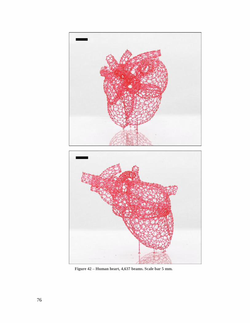
76
Figure 42 – Human heart, 4,637 beams. Scale bar 5 mm.

77
Figure 43 - Sequencing times for each cost function

78
Figure 44 - Heuristic vs. exact compliance for all states

79
As expected, the compliance estimated using the heuristic is always less than or equal to
the exact compliance. Both sequences were successfully used to print all three designs.
Discussion We have developed and validated an approach to generating mechanically robust
assembly sequences for freeform assembly. The algorithm generates an optimal
assembly plan for specific cost functions, but it can also be used to generate good
assembly plans under more general cost functions. Even if an assembly process permits
multiple cantilevers at the same joint, for any cost function related to deformation or
internal beam forces, it is generally preferable to minimize the number and length of
cantilevers present in any given state. The algorithm does this by adding the lowest-cost
consistent subassembly, rather than the lowest-cost single beam. If the applied load is
due to the self-weight of the assembly, adding the lowest-cost single beam will yield a
suboptimal assembly sequence, as shown in an example structure given McEvoy et al.62
Though the algorithm presented here will not in all cases return a global optimum for
loading conditions due to the beams’ self-weight, it returns the optimal sequence for that
particular example. Thus, this approach may be useful for robotic assembly of frame
structures from pre-formed beams as well as for variants of freeform assembly to which
the cantilever constraint does not strictly apply.
The timing for all three constructs was dominated by the time required to compute the
deflections. While obtaining a truly optimal sequence requires solving this system of
equations for every joint at every step, near-optimal sequences can be obtained by
determining the deflection assuming that each root joint of each subassembly tree is
fixed, excluding all non-cantilevered beams from the computation. This allows
generation of assembly sequences in a much shorter time than that required to physically
print the design. However, even using the exact cost function, planning required less time
than the actual printing process for these designs. Because sequencing is initiated from
the empty state, the planner could be run on the fly without the printer ever waiting on the
planner. For even larger designs, however, sequencing using the exact cost function

80
would take longer than printing, and it would be advantageous to use the heuristic cost
function instead.
Our primary motivation for exploring freeform assembly was the applications of round-
channel microchannel networks that can be formed by using the freeform constructs as
sacrificial molds. In the sacrificial molding process, a freeform 3D printed template is
cast in a curable material. Dissolving or otherwise removing the template yields one or
more 3D round channel networks. This can be used to make, for example, 3D
microfluidic devices in materials with tunable optical properties68. A similar approach
could be used to create woven or interpenetrating channel networks in structural
polymers, enabling efficient delivery of 2-part healing chemistries to cracks.69,70 The
ability to incorporate 3D microchannel networks in elastomeric polymers also suggests
applications in integrated microfluidics and soft robotics.71 Round-channel networks are
also useful in recapitulating the structure of native tissue.72-77 Breast and prostate, for
example, contain independent networks of lymphatic, vascular, and ductal channels.
Carcinomas develop in the ducts and metastasize via either the lymphatic or vascular
system; thus, a complete “organ-on-a-chip” model requires all 3 networks. Freeform
assembly can be used to generate this complex topology in a variety of hydrogels, and the
channels can be seeded in a subsequent step.40
Extrusion based bioprinting can directly pattern cells in a single step. If cells are
patterned into a supporting reservoir 17,18, the geometry is relatively unconstrained.
However, it is yet unclear how such an approach would enable oxygen delivery to cells
within the reservoir during long prints. If cells are patterned layer-by-layer, the construct
can be made porous, so that oxygen demand can be met during printing by diffusion from
the gas phase. Printing designs with pores or microchannels is facilitated by
incorporation of a stiff polymer into the construct,31 but it is possible to print a porous
construct using only cell-laden gels as well.16 In the latter case, the pores are backfilled,
and some of the patterned gels are liquefied and removed to create a different vascular
network, better suited to perfusion with liquid media. The chief limitation of these layer-
by-layer approaches is that the gels have low stiffness and must be patterned without

81
cantilevers or long unsupported spans. This limits the topology of the channel networks
that can be created. A highly cited but relatively undeveloped alternative approach is to
print an acellular sacrificial template using water-soluble carbohydrate glass34,37 or
polymer39, then cast a cell-laden hydrogel around it in a single, rapid step. Freeform
assembly with a heated nozzle is a powerful means of patterning these stiff,
biocompatible, water-soluble materials, but improved printing precision and a solution to
the sequencing problem were required to extend this approach to arbitrarily large,
complex designs.
The designs printed here were generated by essentially tracing existing designs or from
discretization of non-uniform rational basis spline surfaces, with some manual tweaking.
Thus, the fully assembled state was specified from the start of the program. However, a
similar graph search approach could be used to generate the topology concurrently with
the sequence. In this case the objective function for any candidate beam would have to
reflect not only the cost (deflection) that would occur during assembly, but also the
benefit of the candidate beam or subassembly with respect to the ultimate function of the
design, i.e., transport of mass or heat.
Conclusion Determining a feasible freeform assembly sequence assembly planning for materials that
stiffen via reversible freezing or glass transition is an NP-complete problem. However,
the issue of exponential run-time can be mitigated by searching for subassemblies that are
“consistent”, meaning they are guaranteed to be consistent with a full assembly sequence
given that one exists. Modeling the assembly as a linear, elastic frame, it is possible to
minimize the greatest error in the position of any joint, ensuring a highly robust sequence.
Assembly plans thus generated perform exceedingly well for patterning isomalt filaments
on the order of 100 μm in diameter. This should facilitate new applications of sacrificial
molding for microfluidics, functional vascularized materials, and tissue engineering, and
may find application in structural engineering as well.

82
Methods
Design Generation The heart design was based off a Solidworks model of a human heart uploaded to
GrabCAD by M.G. Fouché. The surfaces comprising the heart were trimmed and
patched to leave a set of non-manifold surfaces. The SolidWorks Simulation package
was used to generate a triangular mesh for each surface. The mesh was exported to
Mathematica and the centroid of each triangle was connected to form the dual. The
resulting graph was then exported to AutoCAD, where the connected components were
manually joined and the supports were manually added.
The design of the ArcelorMittal Orbit was based off a Sketchup model uploaded to 3D
Warehouse by user Damo. The file was converted to .dxf and modified in AutoCAD to
generate a design suitable for printing. Some pairs of incident beams in the Orbit were
both oriented within about 13° of the vertical, which would make collision unavoidable
for the shape of the nozzles used on the printer. To make the design constructable, the
vertical dimensions of the Orbit were scaled down to 85% of their original value.
The design of the Eiffel tower was based off a .dwg file uploaded to BiblioCAD by user
limazkan. The geometry was used as a guide to create a printable design in AutoCAD.
Algorithm Implementation The search algorithm and direct stiffness method were implemented in Mathematica. The
assembly was modeled as a linear, elastic frame with elements of circular cross-section.
The elastic modulus was set to 2.6 GPa53 and the shear modulus was set to 1.1. This is
based off the assumption that isomalt is linear and isotropic and has a Poisson’s ratio of
0.2, a typical value for glasses. A nominal load of 10-4 Newtons was applied to determine
the stiffness of each joint. The systems of linear equations were solved with Pardiso
5.0.078 integrated within Mathematica. All sequencing was performed on a machine with
a quad core 2.8 GHz intel Core i7 processor and 16 GM of RAM.
Printing
Isomalt Processing Isomalt has a tendency to co-crystallize with water under the heat and shear stress
inherent in melt extrusion processes. This can be prevented by drying the isomalt prior to

83
printing. 50 grams of isomalt (GalenIQ 990, Beneo-Palatinit Gmbh), 25 mg Allura Red
AC (Sigma), and a 3” PTFE stir bar were placed in a 250 mL vacuum flask. The flask
was immersed in a temperature controlled oil bath. The bath was raised to 100°C.
Vacuum was applied using a rotary vane pump. The bath temperature was then ramped to
150 °C at a rate of 120°C/hr. The isomalt was held at 150 °C and stirred at 120 RPM for
2 hours, then cast into an aluminum mold to make a solid rod. The rod was stored under
nitrogen until printing.
Isomalt Printing The isomalt was printed using a custom printer as described previously53,68, using a 110
micron nozzle (Subrex). About 10 g of isomalt was loaded into the extruder barrel and
covered with a layer of pump oil. Designs were printed at 400 μm/s at a pressure of 0.6-
1.2 mPa. The printer has 2 temperature control zones corresponding to the nozzle and the
extruder barrel. The nozzle zone was set to 150° C and the barrel zone was set to 105° C.
The designs were printed onto a substrate of Polyethylene terephthalate, glycol-modified
(PETG). The printer enclosure was continuously purged with dry air from the central
compressed air line, maintaining a relative humidity of less than 20%. After printing,
constructs were stored under nitrogen. However, constructs were photographed under
ambient conditions and showed no apparent degradation over the course of several hours.
Acknowledgements M. K. Gelber was supported by fellowships from the Roy G. Carver Foundation and the
Arnold and Mabel Beckman Foundation. We gratefully acknowledge the gift of isomalt
and advice on its processing provided by Oliver Luhn of Südzucker AG/Beneo-Palatinit
GmbH. The development of the printer was supported by the Beckman Institute for
Advanced Science and Technology via its seed grant program.
We also would like to acknowledge Travis Ross of the Beckman Institute Visualization
laboratory for help with macro photography of the printed constructs. We also thank the
contributors of the CAD files on which we based our designs: GrabCAD user M.G.
Fouche, 3DWarehouse user Damo, and BiblioCAD user limazkan (Javier Mdz). Finally,
We acknowledge Seth Kenkel for valuable feedback on the manuscript.

84
Chapter 5: Mixing in Helical Microchannels Fabricated via Freeform Assembly The following section has been published in Analytical Chemistry. I would like to
acknowledge my co-authors, Matthew R. Kole and Namjung Kim, for their contributions
to this study. Kole built the stimulated Raman microscope and performed the imaging
experiments. Kim performed the simulations.
Introduction
Microfluidic devices allow precise management of small quantities of material, allowing
control and observation of chemical, biological and physical phenomena79. Integral to
their use are microscopy technologies, including optical coherence tomography,80
confocal fluorescence81,82, 2-photon fluorescence83, spontaneous confocal Raman
spectroscopy82,84, and coherent anti-Stokes Raman spectroscopy (CARS). 85,86 Raman
microscopy is particularly attractive because it eliminates the need for exogenous labels,
which may disrupt the native transport properties or other behaviors of the species of
interest in small microfluidic volumes. While the long acquisition times required for
weak spontaneous Raman signals made its use prohibitive, emerging coherent two-
photon Raman microscopies now offer a fast alternative. Stimulated Raman scattering
(SRS) microscopy,87 in particular, can enable quantitative imaging without the
nonspecific background effects and nonlinear analyte response seen in CARS. One
challenge all techniques face is the limiting effect of optical distortion caused by the
microfluidic device features on quantitative accuracy of the measurement. The
microfluidic device‘s interfaces introduce spherical aberration and affect the effective
depth to which the beam(s) focus, the confocal volume changes as a function of depth,
and a reduced collection efficiency often results leading to ‘dark‘ or ‘hidden‘ regions
within the image.88-90 Curved surfaces can additionally introduce lensing effects. The
specific relationship between channel position and optical aberration depends on the
channel depth, the numerical aperture of the illumination/collection optics, the refractive
indices of the chip material and the fluid, and the shape of the interface (Figure 1a),
making quantitative measurements difficult. For wide, shallow channels with a flat
surface perpendicular to the optical axis, changes in image quality across the device tend

85
to be small and can be corrected for91 or neglected92,93. However, for narrow, deep
channels or channels with curved walls, images can be severely distorted. This is quite
obvious in SRS images of a channel with a round cross-section (Figure 1b), and similar
aberrations are apparent in confocal fluorescence microscopy of round cross-section,
helical channels94,95 of a fused silica device. While novel optics have been used to
correct for simple cases96, functional devices can often be sufficiently complex to render
this approach impractical. Recent advances in microfabrication are resulting in complex,
non-planar 3D channels and intricate microfluidic devices that are especially attractive
for a wide range of needs from sophisticated mimicking of physiologic systems97 to
making practical elastomeric valves that completely seal.98 For example, round channels
are required to mimic physiological channel networks, including blood vessels72,74,99,100
and the secretory duct networks in the breast77 and prostate.101 Round channels also have
a minimal ratio of surface area to volume, which minimizes the rate of rate of fouling, the
Figure 45 Aberrations in microfluidic devices do not permit straightforward imaging.
a) Ray-tracing simulation indicating how the features of a microfluidic channel can distort the focal
volume of a confocal/multiphoton imaging technique. Red rays assume a glass (NBK-7) device and a
water-filled channel, while green rays assume the device material has been matched to the refractive
index of water. While spherical aberrations are induced by the air-device interface, the majority of
issues occur from device features. b) Top: SRS image of a cross section of a circular microfluidic
channel without refractive index matching (device and fluid are 1.565 and 1.376, respectively). The
channel cannot be resolved. The horizontal line of dark pixels at the top of the channel is due to a
bubble, which flowed through the channel while those pixels were acquired. Bottom: The fluid has
been changed to RI 1.518, reducing but not eliminating the mismatch between the two components.
The cross section is fully resolved and ‘dark’ regions are significantly reduced. Scale bar = 100 um.

86
pressure required to push a bubble through the channel102, and the pressure drop due to
viscous losses. However, optical imaging of such structures is complicated and there are
no studies to demonstrate that microscopic phenomena can be accurately measured with
high fidelity.
Here we sought to develop an approach to make high fidelity measurements in non-planar
microfluidic devices using non-perturbative two-photon SRS microscopy. We first make
use of a versatile approach to fabricating complex, round-channel microfluidics that is
emerging via the use of 3D printing.5,7,12,37,53,103 This method involves the fabrication of a
sacrificial template, around which a curable material is cast. Realizing that this casting
method is compatible with a wide range of curable materials permitting a wide range of
refractive indices, our method matches the refractive index of the chip itself to the fluid in
the channels. Eliminating refractive index mismatch-dependent aberrations throughout the
device permits imaging without adaptive optics or computation even for complex
geometries. The ability to fabricate and image these complex geometries opens a new
design space for solving many problems in microfluidics, including classical problems
such as mixing in the laminar flow regime. To demonstrate this, we use the sacrificial
molding approach to fabricate a helical micromixer. In a helical or Dean-effect micromixer,
centripetal acceleration of fluid flowing around a curve creates vortices that rotate
transversely to the direction of flow. These Dean vortices can be used to fold the interface
between two adjacent fluid elements, increasing the interfacial area and diffusive transport
between them.104 The magnitude of this effect is related to the Dean number, which is
given by
𝐷𝑒 = 𝑅𝑒√𝑟
𝑅=2𝑄
𝜈𝜋√1
𝑟𝑅
Where Re is the Reynolds number, Q is the mass flow rate, ν is the kinematic viscosity, r
is the radius of the channel cross-section, and R is the radius of curvature. Physically, De
represents the ratio of centripetal forces to viscous forces, and vortex-induced folding of
the fluid interface becomes significant when De is on the order of 1. Though modeling94,105-
107 and some experimental94,108 results indicate that helical designs can create effective

87
passive micromixing devices, there has been no direct comparison of the predicted mixing
profile with experiment, and no comparison of the performance with that of more
conventional mixers fabricated via soft lithography. Hence, we use SRS microscopy to
directly measure chemical distributions of a dissolved species and quantify mixing.
Numerical modeling is used to validate both the imaging results as well as our design
principle and to help understand the mixing process in these devices. The agreement
between experimental and theoretical profiles will demonstrate the fidelity of the
fabrication process as well as the accuracy of visualization using chemical imaging.
Results
Device Fabrication
An overview of the sacrificial template process used and microfluidic mixers made in this
study is shown in Figure 46. Our approach to manufacturing these devices consists of three
steps (Figure 2a). The first step is to directly print the sacrificial 3D template in the shape
of the desired channel network, such that dimensions of the template can be carefully
controlled and channels of considerable complexity can be easily formed. The second step
is to cast the chip material around the template. We lower the template, still attached to the
printing substrate, into a cavity containing a low viscosity polymer precursor. The assembly
is then photocured, encapsulating the template in a cross-linked polymer of well-defined,
homogeneous refractive index and mechanical properties. In the third step, the template is
dissolved away. The chip with the encapsulated template is removed from the printing
substrate. The template is then dissolved by immersing the chip in water, which does not
affect the cross-linked polymer.

88
Figure 46 -3D printing for sacrificial monolithic microfluidic device formation.
(a) The fabrication process consists of three steps. Step 1 is direct printing of a freestanding, 3D
isomalt sacrificial template onto a substrate. In step 2, the template is inverted and placed in a
silicone cavity containing a UV curable resin, which is cured by illuminating through the cavity to
yield a monolithic block encapsulating the template. In step 3, the isomalt is dissolved out of the chip
using water to yield a monolithic device with channels defined by the template.
(b) Photograph during printing of the sacrificial template (video of the printing process in available
in supplementary Movie 1). (c) White light optical image of the finished mixer, with the inset
showing the helical mixer region and measures used to characterize the structure
While several materials can be used to print the template, our preferred material is the sugar
alcohol isomalt, because it is insoluble in the pre-polymer used to form the chip but is
easily dissolved by water in the final step. A still image of the printing process is shown in
Figure 2b and a video of the template printing is provided in supplementary Movie 1.
Though it is possible to print a helical template with any pitch greater than the channel
radius, we chose a relatively large pitch of 500 µm so that in a transmission optical image,
overlap between consecutive half-turns was limited. This facilitated measurement of the

89
minor radius r in the non-overlapping regions (Figure 2c, inset shows the mixing area
magnified). The minor radius r was 78 +/-1.8 µm over the 8.5 turns of the helix and the
major radius helix R was 313 µm. This R is 7.4% smaller than the diameter of the
programmed deposition path and is caused by the constant radial acceleration of the nozzle,
which pulls the small portion of the filament that is still molten towards the center of the
helix. The same effect is observed in other approaches to freeform printed helices109.
Mixing Visualization
Confocal fluorescence microscopy has been used to visualize microfluidic mixing81,82,110,
but the technique presents an inherent problem for non-fluorescent species. Attaching a
bulky fluorescent probe to a chemical can significantly change its physical, chemical and
transport properties in solvents. This makes tagging impractical for many systems, and
impossible for those where the concentration of small molecules or solvents are of interest.
Our system, which comprises epoxy, glucose, NaCl, and water, is one such example - there
no inherent optical contrast between the components and attaching an optical tag to glucose
would be impractical and perturbative. However, these species have different chemical
structures and, therefore, different vibrational spectra. This makes Raman spectroscopic
imaging ideal for directly quantifying the concentration of the non-ionic components at
any given point in the device. Glucose and saltwater show significant spectral differences
in the 2700-3000 cm-1 region arising from the glucose C-H bonds, and so can be easily
separated within the channel. While glucose and epoxy have overlapping spectral features,
they are spatially separated (inside vs outside of the channel). SRS has good depth
sectioning capabilities due to the inherent two-photon nature of the signal; hence, there is
minimal signal overlap between the two compounds. Consequently, we can monitor the
molecule of interest and therefore visualize the flows of the two liquid components in “one
shot” with a single image taken at a Raman shift of 2894 cm-1 .

90
The increase in information content in SRS images as compared to optical microscopy is
apparent. Visualizing cross-sections every ½ helix turn is readily accomplished by
focusing the microscope objective to the center of the mixer and acquiring a single image
along the entire length of the device. 3D images are acquired by z-stack imaging.
(Supplementary Movie 2). Because the intensity of the stimulated Raman scattering is
linearly proportional to the glucose concentration, and the response of the photodiode
detector is linearly proportional to the scattering intensity, the resulting image is
quantitative. The signal intensity recorded from a uniform image of 0% glucose, 5.7% by
weight salt solution was 0.17 V, and the signal intensity recorded from a uniform image
of 8% by weight glucose solution was 0.42 V. Both signals had a standard deviation of
0.03 V. To quantify mixing, we linearly mapped the range 0.17 V to 0.42V between 0
and 1. In order to characterize a more complex system, a sequence of images can probe
multiple Raman shifts.While 3D images can provide visualizations throughout the entire
device, a cross-section of the circular area at various flow rates can illustrate the
progression of mixing within the channel. Figure 48 and Figure 49 show the glucose
concentration at several cross-sections as measured by SRS imaging and compare it to
that predicted by computational modeling.
Figure 47 - Raman spectroscopic characterization and imaging of the chemical constituents and mixers.
(a) Spontaneous Raman spectra of saltwater, glucose solution, and the epoxy used to fabricate the mixer. A
single frequency (2894cm-1, indicated with a dashed line) can be used to differentiate the two solutions
within the channel while the epoxy is spatially distinct. (b) A white-light image of the helix and the
corresponding stimulated Raman intensity image of a single spatial plane (or slice) through the center of the
mixer. Channel cross sections are well resolved with clearly visible concentrations of the glucose solution.
The scale bar indicates 500 µm.

91
Figure 48- Theoretical and experimental comparisons of spatial concentration patterns and
quantification of mixing along the channel.
(a) Experimental (SRS) and simulation (COMSOL) visualizations of glucose concentration at cross
sections in the helical mixer for four different flow rates (Reynolds and Dean numbers also shown). The
SRS images have been scaled to show relative glucose concentration from 0-1, although pixels outside of
this range appear due to noise. In the interest of space only the first 4 turns are shown.
(b) Relative unmixing index as calculated from these cross-section images for experiment and
simulation. Trendlines to the experiment are derived using the best fit for second order polynomials.

92
Figure 49 - Theoretical and experimental comparisons of spatial concentration patterns and
quantification of mixing along the channel.
(a) Experimental (SRS) and simulation (COMSOL) visualizations of glucose concentration at cross
sections in the helical mixer for four different flow rates (Reynolds and Dean numbers also shown). The
SRS images have been scaled to show relative glucose concentration from 0-1, although pixels outside of
this range appear due to noise. In the interest of space only the first 4 turns are shown.
(b) Relative unmixing index as calculated from these cross-section images for experiment and simulation.
Trendlines to the experiment are derived using the best fit for second order polynomials. -
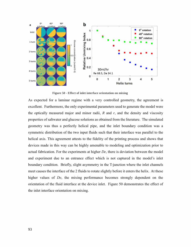
93
As expected for a laminar regime with a very controlled geometry, the agreement is
excellent. Furthermore, the only experimental parameters used to generate the model were
the optically measured major and minor radii, R and r, and the density and viscosity
properties of saltwater and glucose solutions as obtained from the literature. The simulated
geometry was thus a perfectly helical pipe, and the inlet boundary condition was a
symmetric distribution of the two input fluids such that their interface was parallel to the
helical axis. This agreement attests to the fidelity of the printing process and shows that
devices made in this way can be highly amenable to modeling and optimization prior to
actual fabrication. For the experiments at higher De, there is deviation between the model
and experiment due to an entrance effect which is not captured in the model’s inlet
boundary condition. Briefly, slight asymmetry in the T-junction where the inlet channels
meet causes the interface of the 2 fluids to rotate slightly before it enters the helix. At these
higher values of De, the mixing performance becomes strongly dependent on the
orientation of the fluid interface at the device inlet. Figure 50 demonstrates the effect of
the inlet interface orientation on mixing.
Figure 50 - Effect of inlet interface orientation on mixing

94
Performance Analysis
To quantify the extent of mixing we use the relative unmixing index, which is defined as
the ratio of the standard deviation of the pixel intensities at a given cross section to the
standard deviation at the inlet.111 This is mapped to a number between 0 and 1, where 0
represents perfect mixing and 1 no mixing. The evolution of the unmixing index along the
length of our mixer is shown Figure 48 and Figure 49. The close correspondence between
the experimental and theoretical predictions allows us to use numerical modeling to
compare our helical mixer to existing standards of mixing in conventional microfluidics.
For comparison, we use a scaled version of the optimized herringbone mixer design given
by Ansari and Kim.112 We quantified mixer performance in terms of the volume, time, and
pressure drop required to achieve a relative unmixing index of 0.15 (Figure 51 - Relative
performance of helical and herringbone mixers.). We scaled the dimensions of a simulated
herringbone mixer such that the mixer volume and pressure drop were matched for the
herringbone and 3D helical mixers at the same value of Re. This occurred at Re ≈ 10. For
Re < 10, the volume and pressure drop were lower for the herringbone mixer. For Re > 10,
the volume and pressure drop were lower for the helical mixer.
Figure 51 - Relative performance of helical and herringbone mixers.
Data points for mixing length, time, volume, and pressure drop are the ratio of the values required to
obtain 85% mixing for the helical and herringbone devices. Above a Re of 10.2, the helical mixer
requires less time, volume, and pressure to achieve this degree of mixing, and the ratio rises above 1
for all three metrics.

95
At all values of Re, the mixing time was lower for the helical mixer. Thus, for Re > 10,
the simulated helix design outperforms the simulated herringbone design by all three
metrics.
Discussion
Aberration-free imaging is essential to quantitative characterization of microfluidic
devices, including mixers. Mixing is a classical and ubiquitous problem in microfluidic
devices113; though helical mixers have been fabricated in fused silica using femtosecond
laser machining and HF etching,95,114,115 to our knowledge, their performance has not been
well-validated. Our approach addresses this problem by simple 3D fabrication that allows
facile matching of refractive indices90, an approach that has only be used in a few
microfluidic studies.116-119 Our approach enables accurate imaging of the helical mixer, as
evidenced by the close correspondence between the simulated and measured mixing
profiles. At the higher values of De tested (faster fluid flow), entrance effects in the real
mixer skew the inlet concentration profile so that it no longer matches the boundary
condition specified in the simulation. Additionally, at these higher values of De, the flow
profile also transitions from a single vortex to two vortices, with one vortex in the top half
(closer to the inlet) of the cross-section and another vortex in the bottom half (closer to the
outlet). This flow pattern causes effective mixing within each half, but almost no mixing
between the two halves. The result is that at high flow rates the mixing performance is far
better in the model than in the experiment. This discrepancy underscores the value of being
able to directly measure transport in microfluidics even in cases where the underlying
physics are well understood. Even for relatively simple devices, a small error in the
simulation inputs can lead to a large error in the simulation output.
Because microfluidic device fabrication via 3D freeform printing is a significant departure
from more traditional methods, an extant need was to demonstrate that these devices are
capable of performing at approximately the same level as established device designs.
While the helical mixer was chosen due to its difficult-to-image geometry and interesting
flow patterns, its performance was seen to be comparable to the gold standard staggered
herringbone mixer. For Re>10, the simulated helical mixer required less time, less volume,
and a lower pressure drop to achieve a specified unmixing index than did the simulated

96
herringbone mixer. The advantage of the helical mixer at higher Re is due in part to the
circular channel cross-section, which maximizes the hydraulic diameter and thus
minimizes the pressure drop per unit length for a channel of given volume. If the mixer
itself is the only microfluidic component and the flow rate is relatively low, an inefficient
mixer that requires a high input pressure may be acceptable; however, if multiple
components are connected in series, the sum of the pressure drops may be high enough to
cause bonded chips to delaminate and soft PDMS chips to deform.120 Monolithic devices
are immune to failure by delamination, and for devices made of low-stiffness materials, the
lower pressure drop of a helical mixer at higher Re allows for high flow rates and placement
of multiple components in series without risking deformation. For very high pressure
applications, the monolithic casting approach can be used to make mixers with very thick
walls, using very stiff materials. The ability to run chips at very high flow rates, coupled
with the minimization of fouling in a round cross-section, suggests utility in nanoparticle
synthesis, where throughput and fouling have been cited as concerns.121,122 Thus, the these
round-channel devices may afford new opportunities in cases where conventional
microfluidics fall short of current needs121,122.
The ability to rapidly acquire quantitative 3D chemical images presents a new avenue for
characterizing not only mixing, but other aspects of microfluidic device performance as
well. Though we imaged only the effects of advection and diffusion, mass transport in
microfluidics can also be caused by electrical, chemical, thermal, magnetic, or gravitational
potential fields123. When these forces act on a small dissolved species there may be no
suitable probe that can be introduced without changing the behavior of the system. In these
cases, SRS allows direct, label-free acquisition of 3D concentration maps for multiple
analytes. Raman spectroscopy is also sensitive to the formation and destruction of
chemical bonds, to adsorption124, and to conformational changes125. This is valuable in
synthetic and analytical applications in which one needs to capture spatial heterogeneity
within the chip, or when high acquisition speed is required. The demonstration of SRS
imaging for quantifying mixing of a small molecule in solution therefore suggests further
development for monitoring multiple components.

97
Conclusion In this work, we demonstrated full 3D high resolution imaging of flows within a complex
microfluidic device. This was accomplished by two distinct means. First, a fabrication
procedure via sacrificial molding of freeform 3D printed isomalt enables fine control over
the optical properties of the device. This strategy allows for refractive index matching
and the significant reduction of optical aberrations without adjusting the properties of the
fluid. Second, in turn, we demonstrate that stimulated Raman scattering (SRS)
microscopy can be used to directly visualize the concentration of differnet chemical
components within the mixer, without the use of exogenous labels which cannot be
attached to small molecules and may otherwise affect the behavior of relevant species.
We investigated the effect of experimental parameters on mixing performance and show
agreement between experimental results from SRS imaging and numerical solutions of
theoretical models. These results demonstrate a versatile new manufacturing method for
round-channel microfluidics, the ability to accurately simulate the behavior of such
devices during the design phase, an efficient approach to mixing in such devices, and the
utility of SRS as a fast, label-free means for characterizing the operation of microfluidic
devices in general. The principles from this approach should pave the way for analysis of
more complex monitoring in physiologically relevant systems and for accurate
spectroscopic monitoring of reactions in high-flow, low-fouling devices.
Methods
Mixer Fabrication
The helical mixer was fabricated on a 3D printer developed in-house and using a similar
process as described previously.53 A sacrificial template was designed in AutoCAD and
printed on the freeform 3D printer using sugar alcohol isomalt (GalenIQ 990). The isomalt
was heated to 115 °C and extruded through a 55 μm diameter nozzle translated directly
along paths corresponding to the desired channel geometry. The extrusion pressure was
480 kPa, except for the input ports, for which the extrusion pressure was 1930 kPa. A video
of the printing process is available as supplementary Movie 1. The printing speed was 0.2
mm/s and printing took about 6 minutes. A transparent silicone cavity was filled with a
photocurable low refractive index prepolymer (MY-134, My Polymers, Nes Ziona, Israel).

98
The sacrificial template was inverted and placed in the cavity, and the prepolymer was
cured by illuminating both sides of the mold using a mercury lamp for 20 minutes. Upon
release from the cavity, the isomalt was removed by leaving the device in water overnight
at 90 °C.
Modeling
The mixing behavior of the glucose and NaCl solutions was modeled using the COMSOL
Multiphysics Package (COMSOL Group, Stockholm, Sweden). The geometry of the
model was a helix with the same major and minor radii as measured from an optical image
of the device. The pitch and number of turns were the values corresponding to the
programmed printer deposition path. The simulation solved the steady state,
incompressible Navier-Stokes (NS) equation without the external force field for
conservation of mass and momentum:
∇ ∙ 𝑢 = 0
𝜌(𝑢 ∙ ∇)𝑢 = ∇ ∗ [−𝑝𝐼 + 𝜇(∇𝑢 + (∇𝑢)𝑇)]
where u is the velocity, p
is the pressure,
is the density, and
is the viscosity of the
fluid. The use of continuum mechanics is justified by calculation of the Knudsen number
as less than 0.01.126 In addition, the coupled convection-diffusion (CD) equation of a
diluted species was used to model the transport of glucose and NaCl in water, tracking the
location of the interface between two solutions:
∇ ∙ (𝐷∇𝑐) + 𝜇 ∙ ∇𝑐 = 0
where c represents the relative concentration of the sodium and glucose solutions. The
converged solution of NS was fed into CD with the velocity field, and the CD equation
coupled back with the NS equation through the dependence of the density and viscosity on
the relative concentration. We approximated the mixed fluid viscosity and density as a
linear interpolation function between two solutions:
𝜇 = 𝑐𝜇1 + (1 − 𝑐)𝜇2
𝜌 = 𝑐𝜌1 + (1 − 𝑐)𝜌2

99
where the indices 1 and 2 stand for the sodium and glucose solutions, respectively. Values
for viscosity, density, and the diffusion coefficient of 8% by weight glucose and 5.7% by
weight NaCl in water were taken from the literature.127-130 We assumed that the mutual
interaction between two solutions on diffusion coefficient is small enough not to affect the
whole mixing behavior. The no-slip boundary condition on the walls was applied, as is
appropriate for microchannels of hydraulic diameter greater than 30 μm.131_ENREF_131
We used several techniques to reduce the complexity of computational fluid modelling with
µ-level resolution accuracy: 1) The NS and the CD equations were calculated separately to
reduce the computational cost. 2) The computational domain in NS and CD equations was
divided into two parts. For the first part of the domain, the inlet velocity and concentration
profiles were specified, matching the experiment set-up, and the passive outlet boundary
condition (p=0 for NS, or convective flux condition for CD) was applied. The velocity and
concentration profiles at the outlet were exported, and imported as an inlet conditions for
the second part of the domain to complete the results. 3) To improve the convergence of
the simulation, the initial conditions of the high inlet volume flow rate cases were set
through viscosity ramping, starting from higher viscosities (weakly nonlinear problem),
and progressively increasing the nonlinearity until the original problem (highly nonlinear
problem) is solved.
Modeling of the herringbone mixer was performed using the optimized design given in
[42] with W = 380 μm, d/h = 0.48, and θ = 53.2. The mixing time T, pressure drop P, and
mixing volume V, were then determined for a mixer in which W = 480 μm using the
following relations:
𝑇2𝑇1= (
𝑊2𝑊1)2
𝑃2𝑃1= (
𝑊1𝑊2)2
𝑉2𝑉1= (
𝑊2𝑊1)3

100
These scaling relations are derived from the assumption that the mixing profile is purely a
function of the Péclet number. 𝑊2
𝑊1= 1.26 was chosen so that the P and V curves for the
helical mixer crossed the corresponding curves for the herringbone mixer at the same value
of Re.
Stimulated Raman Imaging
All spectroscopic images were acquired using an SRS imaging microscope constructed in
house. The SRS microscope is driven by a dual-output (1064nm/532nm) ultrafast oscillator
coupled into an optical parametric oscillator to provide two picosecond pulse trains whose
wavelength difference can be tuned to match a Raman mode of interest. The imaging was
performed using a long working distance near infrared-corrected objective and a custom-
built single-element photodiode detector. A pair of galvanometer mirrors was used to scan
the focused beams across the specimen during acquisition. For measuring channel cross-
sections, we chose a pixel size of 2μm to be sufficient for clearly resolving the internal
structure. For 3D images of the full mixer acquired via z-stack, we chose a cubic voxel of
5 μm on a side.
Image Processing
All images were processed in Matlab (The Mathworks, Nantucket, MA). Briefly, the
Raman signal from the epoxy is used as an internal standard to account for any
nonuniformity in image intensity due to laser fluctuation or imaging depth. As the epoxy
provides the strongest signal, it can be readily masked out, leaving only the channel cross
sections. The image intensity of each set of cross sections was scaled so that the saltwater
solution at the mixer input had an average value of 0 and the glucose solution at the mixer
input had an average value of 1. In order to compare simulation results to experimental
images, the simulation meshes were mapped onto a square grid of effective pixel size 2μm.
Additionally, the SRS images contain a noise component which the simulation results do
not, and this value was taken into consideration when extracting performance metrics from
the experimental data. The relative unmixing index 𝐼 is given by

101
𝐼 = √
1𝑁∑ (𝑥𝑗 − 𝑥𝑗)
2𝑁𝑗=1
1𝑁∑ (𝑥𝑖 − 𝑥𝑖)2𝑁𝑖=1
Where 𝑥𝑖 are the pixel intensities at the inlet and 𝑥𝑗 the pixel intensities at the cross-section
of interest. We correct for the noise in the image by subtracting the variance due to noise
𝜎𝑛2 from the total variance at each cross-section:
𝐼 = √
1𝑁∑ (𝑥𝑗 − 𝑥𝑗)
2𝑁𝑗=1 − 𝜎𝑛2
1𝑁∑ (𝑥𝑖 − 𝑥𝑖)2𝑁𝑖=1 − 𝜎𝑛2
Acknowledgements We gratefully acknowledge the support of the Beckman Institute for Advanced Science
and Technology via a seed grant for development of the 3D printer. We gratefully
acknowledge the gift of isomalt and advice on its processing provided by Mr. Oliver
Luhn of Suedzucker AG/Beneo-Palatinit GmbH. The development of SRS imaging
methods was supported by NIH via grants R21CA190120 and R01CA197516.

102
Chapter 6: Preliminary Results on Biomedical Applications of Freeform Assembly
Additive Manufacturing of Elastomeric Surgical
Meshes with Spatially Heterogeneous Mechanical
Properties for Pelvic Organ Prolapse
Introduction Pelvic organ prolapse (POP) is the descent of one or more pelvic structures due to
weakening of the supporting pelvic floor muscles, tendons, and fascia. Childbirth often
results in injury to these tissues and to the nerves that innervate the pelvic floor muscles,
with prolapse occurring years or decades later. In some cases, POP may be repaired with
sutures alone. In many cases, however, POP requires an implant to replace the damaged
supportive structures. This implant can be an autologous or cadaverous graft or a
synthetic surgical mesh. Due to the regulatory burden associated with approving new
mesh materials and manufacturing processes, and to the relatively small amount of
federal research dollars allocated to prolapse research, efforts to develop new mesh
materials and manufacturing approaches have been limited. 3D printing is compatible
with many potential mesh materials and enables physicians to design and fabricate
custom meshes at the point of care. In particular, 3D printing enables the rapid patterning
of elastomers, of which the potential advantages in prolapse repair will be discussed.
Data from 1993132 and 1995133 indicate that the lifetime risk of undergoing surgery for
pelvic prolapse or urinary incontinence for a woman in the United States is between 11-
12%, with between 25% and 35% of surgeries performed for urinary incontinence alone.
Data on women in western Australia for the years 2001-2005 suggests a lifetime risk of
pelvic prolapse or urinary incontinence surgery of 19%.134 Data from 2007 to 2011
indicate that the cumulative risk for pelvic prolapse surgery was 12.6% by age 80.135 In
2010, according to industry estimates, about 300,000 women underwent surgery for POP,
of which 100,000 used surgical mesh.136

103
In 2011, the FDA concluded that surgical repair of POP using surgical mesh had not been
shown to improve clinical outcomes over traditional repair using autologous grafts.136
Complications included pain, infection, urinary problems, bleeding, vaginal scarring and
shrinkage, neuromuscular and emotional problems, and mesh erosion through the vaginal
wall. The rate of mesh erosion is about 10% for both synthetic and biological grafts, but
biological graft erosion can be managed without surgery, whereas synthetic graft erosion
requires surgical excision in 67% of cases.137
Factors suggested to influence the probability of graft erosion include the material,
filament structure, pore size, weave, and stiffness.138 Experiments in rhesus macaques
showed that mesh implantation in the vagina causes degeneration in the smooth muscle139
and extracellular matrix 140 of the vagina, and that the degree of degeneration was greater
for a stiffer, heavier, less porous mesh. Degenerated tissue is more susceptible to erosion.
I identify three mechanisms by which surgical mesh could cause the typical
complications: tissue atrophy due to stress shielding, tissue atrophy due to persistent
inflammation, and tissue shrinkage and stiffening due to the development of scar tissue
surrounding the implant.
Stress shielding refers to the tendency of a stiff implant to relieve the mechanical load on
surrounding, more compliant tissues. Stress shielding occurs in bone141, tendons142 and
ligaments143 and could occur in the smooth muscle and extracellular matrix of the vagina.
The absence of mechanical load on the vagina is thought to cause atrophy of the tissue,
leading to bleeding, dyspareunia, and eventually mesh erosion. The better clinical and
experimental139 outcomes associated with less stiff meshes are consistent with the
mechanism of stress shielding. However, unlike bones, tendons, and ligaments, the
vagina is not a load-bearing structure, and it is possible that the pro-degenerative effects
of mesh are mediated by other means.
In this case the degenerative effects of the mesh would be expected to increase with the
contact area of the implant144-146; a mesh with higher porosity would elicit a smaller
degenerative effect, which is also consistent with the findings of those studies.

104
In a successful implant, the implanted material is eventually surrounded by an inert,
fibrotic capsule a few hundred micrometers thick. There is evidence to suggest that
inflammation associated with mesh implantation never completely subsides, and this may
contribute to tissue atrophy. However, the relationship between porosity the
complications of vaginal shrinkage and erosion can also be explained by considering the
mechanical changes induced by fibrosis alone. Fibrosis contracts the surrounding tissue,
causing vaginal shrinkage, and fibrotic tissue is much less compliant than normal tissue.
The implant causes the vagina to shrink and become less elastic. A sudden change in
loading, as might occur while coughing or laughing, would be more likely to cause a tear.
The mechanism of mechanical changes due to fibrosis is also consistent with the finding
that more porous meshes result in fewer complications. predisposing to pain or damage,
especially during intercourse. Furthermore, because fibrosis occurs a few hundred
microns from every filament of the mesh, the extent of fibrosis is determined by the not
only the mesh porosity, but also by the shape of each pore. Mühl et al. presented the idea
of effective porosity, an estimate of the pore area that will ultimately be filled by non-
fibrotic tissue. This is computed by binarizing an image of the mesh and eroding the
pixel blobs corresponding to pores. Thus, the effective porosity of a given mesh is
influenced by pore size: long and thin pores will have low effective porosity, while
circular pores will have maximal effective porosity, even if the area of the pores is the
same for each mesh Although textile meshes can be made highly porous, this porosity is
not always preserved upon implantation. If the mesh is stretched or bent, the pores may
deform, making them longer and narrower and decreasing the effective porosity, as
shown in Figure 52.

105
.
The case for an elastomeric mesh Connective tissue becomes stronger in response to loads placed upon it, and atrophies in
the absence of mechanical stimulus. Though existing surgical meshes bend like
connective tissue, they do not stretch like connective tissue, because their component
fibers are stiff. This can be demonstrated by analyzing one cell of a rectangular mesh,
composed either of a stiff plastic (orange) or an elastomer (blue), as shown in figure 1.
Recently, Lambertz et al. demonstrated that a mesh comprised of knit elastomeric
filaments preserved effective porosity upon implantation for hernia repair.147 The same
would be expected for prolapse repair. This can be explained by considering the
deformation modes of an inelastic and vs. and elastomeric mesh. The former is
97% porosity 97% porosity
40% effective porosity 24% effective porosity
Figure 52 - Effect of deformation on effective porosity

106
dominated by bending; the filaments bend, but their length and diameter remain constant.
Thus, though the mesh will stretch considerably when loaded uniaxially, it will stretch
very little when loaded biaxially. Consider the loading created by a typical ball burst test:
the mesh is anchored at its edges and loaded at its center. The force will initially increase
very slowly, as the slack is taken out of the mesh, and will then increase very rapidly.148
Once the slack is gone and the fibers are completely straight, the modulus of the mesh is
determined the modulus of the individual fibers. For the conventional polypropylene
fibers, this is several GPa – more than an order of magnitude greater than that of muscle
and connective tissue.
In contrast, an elastomeric mesh will deform primarily via stretching. This has two
consequences: closer matching of the tissue and mesh compliance, and preservation of
effective porosity. An elastomeric mesh will more effectively share the load with
surrounding tissue under different deformations. Additionally, the pore shape will be
more constant under these deformations than a conventional mesh. This was shown
experimentally by Lambertz et. al, who used a mesh comprised of elastomeric
polyurethane filaments.147
Figure 53- Ball-burst test

107
Figure 54-Deformation of stiff vs elastic materials
Stress shielding can be decreased by reducing the stiffness of the mesh portion that is
incorporated into the host organs. The foreign body reaction can be minimized by
reducing the contact area of this portion of the mesh and by choosing a highly
biocompatible material. For hernia repair, which is typically done using polypropylene
mesh, the trend has been towards lighter, more porous, more compliant meshes, as it was
shown that the older meshes were much stronger than the abdominal wall itself.149
The clinical trend for POP has also been towards lighter, more porous, more compliant
polypropylene surgical meshes. However, there is a limit to how much material can be
removed from the mesh before its function is compromised. Although the mesh should
be highly porous and compliant in the areas in which it is in contact with the rectum,
bladder, and vagina, the supporting straps need to be stiff enough to provide sufficient
support to the endopelvic fascia. Another concern is handling: stiffer meshes tend to be
easier to place during surgery. Some newer surgical meshes incorporate a stiff,
resorbable component for this reason.
Material It would appear that the ideal mesh for POP would have spatially heterogeneous
mechanical properties. The choice of material depends on the relative contributions of
Uniaxial Loading
Stiff material, e.g.,
polypropylene
Tendon or
elastomer
Unloaded

108
two factors to the risk of erosion: the foreign body reaction and stress shielding. Stress
shielding is caused by a mismatch between tissue and implant stiffness. However, the
stiffness of the mesh is an extensive property, which can be reduced simply by removing
more material. For example, a mesh material with a modulus of 2 GPa and a porosity of
75% would have the same stiffness as a mesh material with a modulus of 1 GPa and a
porosity of 50%.
If mesh erosion is due entirely to stress shielding, any material can be used provided it is
sufficiently strong and resistant to fatigue. Porosity is a free variable and can be used to
control the modulus across the mesh. However, if mesh erosion is due entirely to the
foreign body reaction, then both material stiffness and biocompatibility must be
considered. A very high modulus material will allow a mesh to be constructed with less
total material, reducing the interfacial area between the tissue and implant, thus
attenuating the foreign body reaction. On the other hand, a lower modulus material,
which requires a lower porosity, may be the better choice if it evokes a much milder
foreign body response.
Research in biodegradable elastomers increased greatly after 2002 with the synthesis of
poly(glycerol-sebacate) (PGS).150 Recently, Langer and others reported a variant of PGS,
poly (glycerol sebacate urethane) (PGSU), with greatly improved mechanical and
degradation properties.151 Briefly summarizing the main points of the paper:
PGSU films are easily manipulated and sutured
Implanted PGSU films induce minimal inflammation and minimal fibrosis
Proteins or other bioactive molecules can be loaded into porous PGSU during
synthesis
PGSU can be synthesized quickly (<36 hours) using low-cost reagents
The stiffness and degradation time of PGSU increase with the degree of cross-
linking, which is controllable during synthesis
PGSU does not swell or shrink appreciably in physiological solutions
PGSU can be autoclaved without major changes in material properties
109
PGSU maintains its tensile properties throughout cyclic loading with minimal
creep
For a solid film or sheet, mesh compliance C (measured in cm/N) and modulus of
elasticity ε (measured in N/cm2) are related by the following equation:
𝐶 =1
휀𝑡(1 − 𝑃)
Where t is the thickness of the material in cm and P is the porosity. Thus, a 0.05 cm
sheet of 0% porosity will require a modulus between 222 and 1,000 N/cm2, or between 2
and 10 MPa, and a tensile strength between 2.2 and 6 MPa. The modulus of PGSU can be
tuned from 0.1 to 20 MPa by changing the degree of cross-linking, and the compliance
can be further tuned by changing the mesh thickness or porosity. For samples with a
modulus between 4.5 and 10 MPa, tensile strength is between 2.8 and 7 MPa; according
to the data in the paper, any sample of PGSU that has the desired compliance will be
sufficiently strong as well.
Degradation time increases with the degree of cross-linking. Because PGSU degrades via
surface erosion, degradation time can be decreased by increasing the ratio of surface area
to volume – i.e., by making holes in the mesh and increasing the porosity. A large
number of small holes will increase the surface area more than a small number of large
holes, resulting in faster degradation.
A functional “mesh” design could simply be a sheet of PGSU. Solvent-polymerized
PGSU with a 1:0.5 ratio of pre-polymer to cross-linker lost 32% of its weight over 20
weeks and was fragmented at 40 weeks. A 0.5 mm thick, non-porous sheet of this sample
would meet the specifications for compliance and tensile strength and be extremely easy
to fabricate.
The density of PGS is about 1.2 g/cm3.152 Assuming the density of PGSU is similar to
that of PGS, a 0.5 mm thick sheet of 0% porosity would weigh 600 g/m2 – far greater
than the 25 g/m2 target. Using the stiffest sample reported in the paper, the mesh could be
made with up to 90% porosity, weigh as little as 60 g/ m2, and meet the specification for

110
compliance. Achieving the 25 g/m2 target would require a more highly cross-linked
sample than was reported in the paper, but this is certainly possible. Of course, the mesh
is 100% absorbable, so the post-absorption weight (0 g) meets the weight target.
Cell Seeding and Collagen Deposition PGSU supports adhesion of human mesenchymal stem cells.151 PGS supports adhesion
and proliferation of human foreskin fibroblasts152. These PGS scaffolds accumulate
collagen, and I would expect the same to be true of PGSU.
Collagen fibers are known to align under cyclic loading, resulting in increased strength
and stiffness in the direction of strain.153 Using a non-elastomeric mesh shields the native
tissue from cyclic loading, but new tissue growing on the mesh may be shielded as well.
If the mesh deformation is primarily via bending, the infiltrating tissue will not “see” the
tensile strain and will fail to remodel accordingly. Using an elastomer like PGSU ensures
that strain is transferred to any infiltrating tissue, and should result in a stronger support
structure than could be grown on a non-elastomeric scaffold. PGS scaffolds have been
successfully implanted in rats as a nerve conduit154, subcutaneously,155 as an arterial
graft156, and as a heart patch.157 PGSU was implanted subcutaneously in rats, and resulted
in minimal inflammation and fibrosis (much less than poly (lactic-co-glycolic acid),
PLGA). Thus, although PGS and PGSU have not been approved for use in humans, there
is evidence that they are safe, and even superior to approved polymers such as PLGA.
Generating a design One way to create a mesh with spatially varying mechanical properties is to spatially
modulate the properties of the material itself. However, this would require either joining
meshes with different properties, or chemically or physically modifying the mesh
material at different locations after the mesh is made. Conventional knitting techniques
create a homogenous mesh structure across the entire textile. While a sophisticated
knitting process may be able to produce textiles with stiffness and porosity in different
parts of the mesh, this has not to our knowledge been demonstrated.
Direct printing of surgical mesh offers a simple means of spatially modulating the
mechanical properties of the mesh through control of the topology. Although there are a
number of known approaches for optimizing topology of truss networks under known

111
loading conditions158, the optimality criteria for surgical mesh also includes the mesh
effective porosity.147,159 In order to prevent complete encapsulation of the mesh by
fibrotic tissue, the mesh should have holes that are as large and as nearly circular as
possible. A natural means of producing such a pattern is by defining the centers of the
pores, then defining the filaments as the edges of the corresponding Voronoi cells. The
local stiffness of the mesh then is correlated to the spatial density of the pore centers.
This approach is maximizes effective porosity and enables rapid iteration on mesh
design. The density and direction of filaments can be chosen to impart the desired
porosity and stiffness. Stiffness can be a function of angle as well as position. We shall
consider the control of topology alone using filaments of uniform cross-section. The
mesh is designed as follows.
1) The mesh regions are drawn and assigned a node density, which will determine
the porosity of the final mesh.
2) The mesh nodes are generated using methods known from finite element analysis.
3) The Voronoi diagram of the mesh nodes is computed. Lines extending beyond
the boundaries of the mesh are deleted.
The process for topology generation of a transvaginal mesh is shown in Figure 55.
For elastomeric meshes, conventional mesh fabrication approaches like knitting are not
necessarily the best solution. Elastomers like PGSU can be molded, but the intricate
features can complicate de-molding. An interesting alternative for manufacturing these
meshes is freeform assembly, albeit the degenerate, 2D case. Assembly planning in this
case is a very different problem; stability is not a concern, and the metric of interest is
speed.

112
Freeform assembly, An interesting alternative to subtractive processes is additive
Figure 55 – Mesh Regions.
Node density is indicated by color in the order red, yellow, green, blue, with red representing the highest node
density.
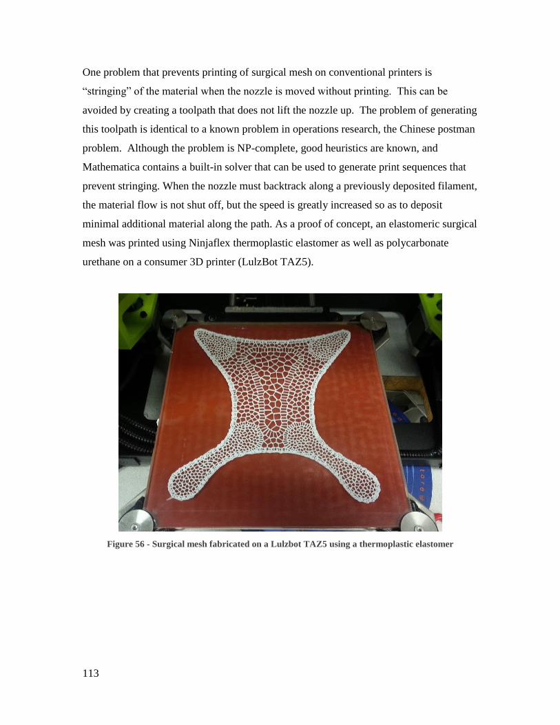
113
One problem that prevents printing of surgical mesh on conventional printers is
“stringing” of the material when the nozzle is moved without printing. This can be
avoided by creating a toolpath that does not lift the nozzle up. The problem of generating
this toolpath is identical to a known problem in operations research, the Chinese postman
problem. Although the problem is NP-complete, good heuristics are known, and
Mathematica contains a built-in solver that can be used to generate print sequences that
prevent stringing. When the nozzle must backtrack along a previously deposited filament,
the material flow is not shut off, but the speed is greatly increased so as to deposit
minimal additional material along the path. As a proof of concept, an elastomeric surgical
mesh was printed using Ninjaflex thermoplastic elastomer as well as polycarbonate
urethane on a consumer 3D printer (LulzBot TAZ5).
Figure 56 - Surgical mesh fabricated on a Lulzbot TAZ5 using a thermoplastic elastomer

114
Figure 57 – Printed elastomeric surgical mesh
Conclusion Pelvic organ prolapse (POP) surgical repair using existing surgical meshes and native
tissue augmentation results in unacceptable rates of complications and reoperation.
Ideally, a mesh implant would provide temporary support to the pelvic organs while
allowing some of the loading to be transferred to the pubic ligaments and fascia. I
hypothesize that the compliance of a plastic surgical mesh measured using a uniaxial
tension test overestimates the actual compliance of an implanted mesh, which is anchored
at four or more points. Existing meshes cause stress shielding because they bend, but
under multiaxial loading, they don’t stretch.
To solve this problem I suggest that the mesh be made of a biodegradable elastomer, poly
(glycerol sebacate urethane) (PGSU). Using an elastomer like PGSU it is possible to
make a mesh that actually stretches like collagenous tissue, rather than simply bends like
existing plastic meshes. This will more effectively transfer some of the load to existing
connective tissue, preventing stress shielding and atrophy. PGSU is inexpensive, causes
minimal inflammation, and supports cell seeding. Its softness greatly reduces the
probability of erosion and eliminates the possibility of perforation.

115
On-demand Fabrication of Resorbable Polymer Stents
Background Historically, stents have been machined or woven from metal alloys. However, there are
a number of problems associated with these permanent stents. Permanent stents may
inhibit full remodeling of vasculature160 and cause stent thrombosis several years after
implantation161 . If a permanent stent breaks, a fragment may migrate and cause
complications elsewhere in the body.162
These problems have motivated the development of resorbable polymer stents.
Resorbable stents reduce the risk of late stent thrombosis and breakage, and can easily be
doped with anti-inflammatory or anti-thrombotic drugs, which are released for as long as
the stent is present. However, making a polymer stent that is as strong as a metal stent
remains challenging, and polymer stents, like metal stents, are manufactured in discrete
sizes and shapes. Stents are not personalized. There is currently no solution for tailoring
the stent geometry, strength, compliance, drug loading, or degradation rate to the patient.
Freeform assembly is a natural means of making tailored stents.
Figure 58 –Image of the nozzle depositing the struts (left) and a finished bifurcating stent (right).

116
Figure 59 - 3D-printed balloon-expandable polymer stents.
The lower stent is loaded onto a balloon catheter.
Proposal One patient population that could benefit from the development of 3D printed stents is
those with carotid stenosis, a risk factor for stroke. Carotid stenosis typically occurs
where the common carotid divides into the internal and external carotid arteries, and is
treated by either surgery (endarterectomy) or stenting, with comparable outcomes.163
Stenting is much less invasive, and could potentially be performed on many more
patients, but improvements in stents and stenting procedures are necessary in order for
carotid stenting to show greater safety and efficacy than endarterectomy.
Whereas cardiac stenting is often an emergency procedure, carotid stenosis, even in
severe cases, need not be treated immediately. During a routine screening, a physician
would image a patient’s carotid arteries using Doppler ultrasound, magnetic resonance
angiography, or computed tomography angiography. If the patient is deemed at risk for
stroke, we would then design a stent based on the image data, print it, and perform

117
quality control measures. The physician would receive a stent custom-built for the
patient a few days after the initial examination.
This printed stent would be optimized in size, shape, and compliance. Using a stent
designed to fit a specific patient’s carotid bifurcation would make the implantation
process easier, reducing the risk of complications and allowing more procedures to be
performed in a shorter time. Stent compliance can be tuned as well: by making struts of
variable diameter, the stent can be made stiff in the middle to prevent crushing and
flexible at the ends to match the compliance of artery wall. The abrupt change in
compliance at the boundary of a stiff stent causes aberrant hemodynamics, promoting
restenosis.164 A matched-compliance stent solves this problem.
Eventually the technology would be developed to the extent that stents could be produced
on-demand at the point of care. Software would use image data determine the
appropriate dimensions for the stent and generate a design algorithmically. The stent
would then be printed in minutes, at the hospital.
Some problems remain to be solved. For example, delivery of a bifurcating stent via
catheter requires some engineering in and of itself. Future work will include identifying
and meeting the clinical requirements of a 3D printed stent as well as validating the stent
in a porcine model.

118
Towards a culture model of the kidney proximal tubule
Background Modeling drug clearance from the proximal tubule is a significant problem in drug
discovery. Animal models are inconvenient, and existing in vitro models fail to
recapitulate the structure and function of real tissue. This section outlines a protocol for
engineering a proximal tubule and its peritubular capillary network using a microfluidic
hydrogel fabricated via a 3D-printing process. A proximal tubule channel and two
flanking vascular channels are first formed in a collagen gel with dispersed pericytes.
The channels are then seeded with the appropriate endothelia, and a microvascular
network is grown between the vascular channels flanking the proximal tubule. This
culture system mimics the in vivo configuration of the proximal tubule and enables
perfusion of the tubule as well as the associated microvascular network. Drug clearance
through the tubule wall can be assayed by sampling the medium used to perfuse the
microvascular network, providing a biological readout that does not perturb the culture
model.
In the embryo, nephron tubulogenesis occurs via a mesenchymal to epithelial
transition.165 This is fundamentally different from the branching morphogenesis that
produces most epithelialized tissue, and while branching morphogenesis can be readily
induced to create epithelialized tubule networks of many different tissues, the nephron is
not one of them.166 Some groups have attempted to mimic the embryonic development of
the nephron in vitro using mesenchymal stem cells, but this approach does not appear
sufficiently developed for industrial use.167 Although de novo tubulogenesis of the
proximal tubule is not yet possible, mature tubular cells form a correctly polarized
epithelial layer with tight junctions if cultured on collagen IV or laminin.168 Making a
tubule should thus be possible simply by seeding the inside of a collagen IV or laminin
coated lumen with proximal tubule epithelial cells. The peritubular capillaries can then
be grown around the tubule using established techniques,169,170 provided the tubule is
formed in a hydrogel that supports angiogenesis. Both the tubule and vasculature must
then connected to external tubing and perfused.

119
The proximal tubule is a hollow cylinder about 65 µm in diameter and about 14 mm long.
Making a 65 µm diameter lumen in a soft hydrogel, then attaching external tubing, is not
trivial. Sacrificial molding using an isomalt mold fabricated via freeform assembly is a
promising part of the solution. A complete protocol is outlined below.
Proposal 1) 3D print sacrificial material
The tubule and flanking vascular channels will be formed by removing sacrificial
materials patterned in 3D within a bulk gel. Figure 60 shows the sacrificial
pattern. The upright filaments, which will form the tubing connections, are 400
µm in diameter, and the meandering filaments are 65 µm in diameter. The middle
filament will ultimately form the lumen of the proximal tubule. The flanking
filaments will be used to grow the microvasculature.
The freestanding mold shown below would be manufactured using freeform 3D
printing. This type of mold must reportedly be coated with a polymer layer a few
µm thick to prevent the sacrificial material from dissolving before gelation
occurs.53 The polymer layer supports mass transport of large molecules37, but it
likely creates an impermeable barrier to endothelial cells, which cannot sprout
through the polymer to form the microvascular network. The authors of [10]
suggest some solutions to this problem. Alternatively, channels can be formed via
the fugitive ink method, in which sacrificial material is printed directly into the
gel.15
Figure 60 - Sacrificial mold

120
2) Cast mold in collagen I gel with dispersed pericytes.
Collagen I is selected because it is known to support angiogenesis under the
influence of a chemically defined vasculogenesis medium.170 Pericytes can be
suspended in fibrin gel at 5x10⁶ cells/ml,169 and the same should be possible with
collagen I. The culture container shown below is filled with about 35 µL of
neutralized 1% collagen I solution containing pericytes at a concentration of
5x10⁶ cells/ml. The substrate is inverted and the sacrificial mold is submerged in
the solution. The solution is gelled in an incubator at 37° for 30 minutes as
described.170
Figure 61 - Casting of cell-laden gel
3) Remove sacrificial material
Water soluble sacrificial material is removed by dissolution. Liver cells dispersed
in microfluidic hydrogels formed by this process retain high viability37, and the
sacrificial material should be compatible with pericytes as well. If the osmotic
pressure increase caused by the dissolving sacrificial material has a negative
effect on the pericytes, culture medium can be flowed through the 2 small holes in
the substrate to dilute the dissolved sacrificial material.
If fugitive ink is used instead of sacrificial molding, the ink must be removed by
applying pressure. This is more easily done if the fluidic connections are
attached, as described next.

121
Figure 62 – Mold dissolution
4) Insert and lock tube connections
The channels are connected to external tubing through a pre-built adapter. The
adapter is aligned using shoulder screws and lowered such that each tube
connection enters the corresponding port in the gel. In order to seal the tube
connections, additional gel or silicone is added on top of the existing gel through
the 2 tubes in the middle of the adapter.
Figure 63 - Fluidic interfaces
5) Coat proximal tubule with collagen IV or laminin

122
Kidney proximal tubule cells fail to develop tight junctions when cultured on a
collagen I substrate, but will develop tight junctions when grown on basement
membrane proteins collagen IV or laminin.168 One solution to this problem is to
form the entire gel from basement membrane. The protocol for vascularization
calls for collagen I, but it may work with these gels as well. Another solution is
to coat the proximal tubule channel with basement membrane via viscous
fingering. This is done by flowing a high-viscosity solution of basement
membrane proteins through the channel, followed by a low-viscosity fluid like
culture medium.171
Figure 64 -ECM coating
6) Seed proximal tubule
Proximal tubule epithelial cells are suspended in culture medium and flowed
through the central channel to seed it.
Figure 65 – Proximal tubule endothelium seeding
7) Seed vascular channels
Vascular endothelium can be cultured directly on collagen I, so the vascular
channels can be seeded without coating. Human vascular endothelial cells are
suspended in culture medium and flowed through the flanking channels to form
two endothelialized vessels from which angiogenesis can proceed.
Collagen IV or laminin
followed by culture medium
Proximal tubule
endothelial cells

123
Figure 66 - Vascular endothelium seeding
8) Grow microvascular network
The microvascular network is grown between the two vascular channels.
Vasculogenesis medium is flowed through one of the channels, and ordinary
culture medium is flowed through the other channel. The gradient of VEGF and
other angiogenic factors in the vasculogenesis medium induces sprouting from the
channel on the low end of the gradient.170
Figure 67 - Gradient formation to induce vasculogenesis
Discussion This process forms a cylindrical channel in an ECM-mimicking hydrogel containing
pericytes. The channel walls are seeded with proximal tubule epithelia, yielding a
monolayer of tubular epithelia surrounding a round lumen. The length and diameter of
the engineered tubule are chosen to match those of the proximal tubule in vivo. The
peritubular network is then grown around this channel using vascular endothelial cells.
This yields a physiological configuration of all three cell types.Proximal tubule
epithelium grown on ECM substrates is viable for 2-3 weeks in culture.168 Microvascular
networks grown in collagen I permit multiweek cultures172, and pericytes remain viable
for at least 3 weeks in culture.173 There is some space on top of the gel in the culture
chamber to which culture medium can be added. Alternatively, the culture can be
perfused through the vascular channels. Flow must initially be directed along each
channel, parallel to the tubule. After the microvascular network is grown and connects
Vasculogenesis medium
Culture medium
Vascular
endothelial cells

124
the two vascular channels, flow can be directed through the grown network, from one
vascular channel to the other. Pressure can be provided using an external syringe pump,
an elevated IV bag, or a peristaltic pump. Tubular epithelium cultured on ECM proteins
displays the correct polarity, forms tight junctions, and expresses the characteristic
proteins.168 Apical shear stress enhances polarization and the formation of cilia.174 This
culture model allows for flow over an epithelial monolayer cultured on ECM proteins,
and so should perform as well as existing systems that grow tubular epithelium under
these conditions. This model allows perfusion of both the tubule and the associated
capillary network. The amount of PAH (para-aminohippuric acid ) or any other analyte
flowed through the tubule can thus be measured in the “blood”, i.e., the vascular
perfusion medium.
This proposal was submitted as part of an Innocentive open innovation proposal in June
2015. Since then, a similar printing process175 has been used to create a model of the
kidney proximal tubule, albeit without a microvascular network. In that study, the tubule
lumen was formed by printing a fugitive ink onto a layer of fibroblast-laden gelatin-fibrin
hydrogel, then covered with another layer of this hydrogel. Because cells were not
printed directly, a free-standing sacrificial mold could likely be substituted directly into
that protocol. The resulting construct should be identical, but the workflow is somewhat
simplified using a freestanding sacrificial mold, because the printing step is entirely
separate from the casting step.

125
References 1 Zhu, C. & Smay, J. E. Catenary shape evolution of spanning structures in direct-
write assembly of colloidal gels. Journal of Materials Processing Technology
212, 727-733, doi:http://dx.doi.org/10.1016/j.jmatprotec.2011.04.005 (2012).
2 Gratson, G. M. & Lewis, J. A. Phase behavior and rheological properties of
polyelectrolyte inks for direct-write assembly. Langmuir 21, 457-464,
doi:10.1021/la048228d (2005).
3 Xu, M. & Lewis, J. A. Phase behavior and rheological properties of polyamine-
rich complexes for direct-write assembly. Langmuir 23, 12752-12759,
doi:10.1021/la702249u (2007).
4 Ghosh, S., Parker, S. T., Wang, X., Kaplan, D. L. & Lewis, J. A. Direct-write
assembly of microperiodic silk fibroin scaffolds for tissue engineering
applications. Adv. Funct. Mater. 18, 1883-1889, doi:10.1002/adfm.200800040
(2008).
5 Wu, W. et al. Direct-write assembly of biomimetic microvascular networks for
efficient fluid transport. Soft Matter 6, 739-742, doi:10.1039/b918436h (2010).
6 Smay, J. E., Cesarano, J. & Lewis, J. A. Colloidal Inks for Directed Assembly of
3-D Periodic Structures. Langmuir 18, 5429-5437, doi:10.1021/la0257135 (2002).
7 Therriault, D., White, S. R. & Lewis, J. A. Chaotic mixing in three-dimensional
microvascular networks fabricated by direct-write assembly. Nat Mater 2, 265-
271 (2003).
8 Lewis, J. A. & Gratson, G. M. Direct writing in three dimensions. Materials
Today 7, 32-39, doi:http://dx.doi.org/10.1016/S1369-7021(04)00344-X (2004).
9 Li, Q. & Lewis, J. A. Nanoparticle Inks for Directed Assembly of Three-
Dimensional Periodic Structures. Adv. Mater. 15, 1639-1643,
doi:10.1002/adma.200305413 (2003).
10 Therriault, D., Shepherd, R. F., White, S. R. & Lewis, J. A. Fugitive inks for
direct-write assembly of three-dimensional microvascular networks. Adv. Mater.
17, 395-399, doi:10.1002/adma.200400481 (2005).
11 Gratson, G. M. et al. Direct-write assembly of three-dimensional photonic
crystals: Conversion of polymer scaffolds to silicon hollow-woodpile structures.
Adv. Mater. 18, 461-465, doi:10.1002/adma.200501447 (2006).
12 Toohey, K. S., Sottos, N. R., Lewis, J. A., Moore, J. S. & White, S. R. Self-
healing materials with microvascular networks. Nat Mater 6, 581-585 (2007).
13 Ahn, B. Y. et al. Omnidirectional Printing of Flexible, Stretchable, and Spanning
Silver Microelectrodes. Science 323, 1590-1593, doi:10.1126/science.1168375
(2009).
14 Wu, W., DeConinck, A. & Lewis, J. A. Omnidirectional Printing of 3D
Microvascular Networks. Adv. Mater. 23, H178-H183,
doi:10.1002/adma.201004625 (2011).
15 Kolesky, D. B. et al. 3D Bioprinting of Vascularized, Heterogeneous Cell-Laden
Tissue Constructs. Adv. Mater. 26, 3124-3130, doi:10.1002/adma.201305506
(2014).

126
16 Kolesky, D. B., Homan, K. A., Skylar-Scott, M. A. & Lewis, J. A. Three-
dimensional bioprinting of thick vascularized tissues. Proc. Natl. Acad. Sci.
U.S.A. 113, 3179-3184, doi:10.1073/pnas.1521342113 (2016).
17 Bhattacharjee, T. et al. Writing in the granular gel medium. Science Advances 1,
doi:10.1126/sciadv.1500655 (2015).
18 Hinton, T. J. et al. Three-dimensional printing of complex biological structures by
freeform reversible embedding of suspended hydrogels. Science Advances 1,
doi:10.1126/sciadv.1500758 (2015).
19 Yamada, A., Niikura, F. & Ikuta, K. A three-dimensional microfabrication system
for biodegradable polymers with high resolution and biocompatibility. Journal of
Micromechanics and Microengineering 18, 025035 (2008).
20 Hack, N. & Lauer, W. V. Mesh-Mould: Robotically Fabricated Spatial Meshes as
Reinforced Concrete Formwork. Architectural Design 84, 44-53,
doi:10.1002/ad.1753 (2014).
21 Technology, B. <http://www.branch.technology/> (2015).
22 Mueller, S. et al. in Proceedings of the 27th annual ACM symposium on User
interface software and technology 273-280 (ACM, Honolulu, Hawaii, USA,
2014).
23 A Radically New 3D Printing Method, <http://www.mataerial.com/#description>
(
24 Lebel, L. L., Aissa, B., Khakani, M. A. E. & Therriault, D. Ultraviolet-Assisted
Direct-Write Fabrication of Carbon Nanotube/Polymer Nanocomposite
Microcoils. Adv. Mater. 22, 592-596, doi:10.1002/adma.200902192 (2010).
25 Farahani, R. D. et al. Direct-write fabrication of freestanding nanocomposite
strain sensors. Nanotechnology 23, 085502, doi:10.1088/0957-4484/23/8/085502
(2012).
26 Skylar-Scott, M. A., Gunasekaran, S. & Lewis, J. A. Laser-assisted direct ink
writing of planar and 3D metal architectures. PNAS (2016).
27 Guo, S.-Z. et al. Solvent-Cast Three-Dimensional Printing of Multifunctional
Microsystems. Small 9, 4118-4122, doi:10.1002/smll.201300975 (2013).
28 Guo, S.-Z., Heuzey, M.-C. & Therriault, D. Properties of Polylactide Inks for
Solvent-Cast Printing of Three-Dimensional Freeform Microstructures. Langmuir
30, 1142-1150, doi:10.1021/la4036425 (2014).
29 Printing outside the box, <http://mx3d.com/> (
30 Korecky, B., Hai, C. M. & Rakusan, K. Functional capillary density in normal
and transplanted rat hearts. Can J Physiol Pharmacol 60, 23-32 (1982).
31 Kang, H.-W. et al. A 3D bioprinting system to produce human-scale tissue
constructs with structural integrity. Nat Biotech 34, 312-319,
doi:10.1038/nbt.3413
http://www.nature.com/nbt/journal/v34/n3/abs/nbt.3413.html#supplementary-information
(2016).
32 Oh, S. H., Ward, C. L., Atala, A., Yoo, J. J. & Harrison, B. S. Oxygen generating
scaffolds for enhancing engineered tissue survival. Biomaterials 30, 757-762,
doi:10.1016/j.biomaterials.2008.09.065 (2009).

127
33 Jaeger, A. A. et al. Microfabricated polymeric vessel mimetics for 3-D cancer cell
culture. Biomaterials 34, 8301-8313, doi:10.1016/j.biomaterials.2013.07.013
(2013).
34 Bellan, L. M. et al. Fabrication of an artificial 3-dimensional vascular network
using sacrificial sugar structures. Soft Matter 5, 1354-1357,
doi:10.1039/b819905a (2009).
35 Bellan, L. M. et al. Fabrication of a Hybrid Microfluidic System Incorporating
both Lithographically Patterned Microchannels and a 3D Fiber-Formed
Microfluidic Network. Advanced Healthcare Materials 1, 164-167,
doi:10.1002/adhm.201100052 (2012).
36 Bellan, L. M., Pearsall, M., Cropek, D. M. & Langer, R. A 3D Interconnected
Microchannel Network Formed in Gelatin by Sacrificial Shellac Microfibers. Adv.
Mater. 24, 5187-5191, doi:10.1002/adma.201200810 (2012).
37 Miller, J. S. et al. Rapid casting of patterned vascular networks for perfusable
engineered three-dimensional tissues. Nat Mater 11, 768-774 (2012).
38 Bertassoni, L. E. et al. Hydrogel bioprinted microchannel networks for
vascularization of tissue engineering constructs. Lab. Chip 14, 2202-2211,
doi:10.1039/c4lc00030g (2014).
39 Mohanty, S. et al. Fabrication of scalable and structured tissue engineering
scaffolds using water dissolvable sacrificial 3D printed moulds. Materials Science
and Engineering: C 55, 569-578,
doi:http://dx.doi.org/10.1016/j.msec.2015.06.002 (2015).
40 Kinstlinger, I. S. & Miller, J. S. 3D-printed fluidic networks as vasculature for
engineered tissue. Lab. Chip 16, 2025-2043, doi:10.1039/c6lc00193a (2016).
41 Hartel, R. W., Ergun, R. & Vogel, S. Phase/State Transitions of Confectionery
Sweeteners: Thermodynamic and Kinetic Aspects. Comprehensive Reviews in
Food Science and Food Safety 10, 17-32, doi:10.1111/j.1541-4337.2010.00136.x
(2011).
42 Blander, M. & Katz, J. L. Bubble nucleation in liquids. AIChE J. 21, 833-848
(1975).
43 Kim, S. H. & Chu, C. C. Fabrication of a biodegradable polysaccharide hydrogel
with riboflavin, vitamin B2, as a photo-initiator and L-arginine as coinitiator upon
UV irradiation. J. Biomed. Mater. Res. B Appl. Biomater. 91, 390-400,
doi:10.1002/jbm.b.31414 (2009).
44 Therriault, D., White, S. R. & Lewis, J. A. Rheological behavior of fugitive
organic inks for direct-write assembly. Applied Rheology 17, 10112-10111-
10112-10118 (2007).
45 Buckmaster, J. D., Nachman, A. & Ting, L. The buckling and stretching of a
viscida. J. Fluid Mech. 69, 1-20, doi:10.1017/s0022112075001279 (1975).
46 Chiu-Webster, S. & Lister, J. R. The fall of a viscous thread onto a moving
surface: a ‘fluid-mechanical sewing machine’. J. Fluid Mech. 569, 89-111,
doi:10.1017/s0022112006002503 (2006).
47 Teichman, J. & Mahadevan, L. The viscous catenary. J. Fluid Mech. 478, 71-80
(2003).
48 Andersson, O. & Johari, G. P. Thermal conductivity of Glycerol’s liquid, glass,
and crystal states, glass-liquid-glass transition, and crystallization at high

128
pressures. The Journal of Chemical Physics 144, 064504, doi:10.1063/1.4941335
(2016).
49 Incropera, F. P. & DeWitt, D. P. Fundamentals of heat and mass transfer. 5th ed.
edn, xix, 981 pages : illustrations (some color) ; 26 cm + 1 computer disc (4 3/4
in.) with user's guide (J. Wiley, 2002).
50 Eötvös, R. Ueber den Zusammenhang der Oberflächenspannung der Flüssigkeiten
mit ihrem Molecularvolumen. Annalen der Physik 263, 448-459,
doi:10.1002/andp.18862630309 (1886).
51 Trouton, F. T. On the Coefficient of Viscous Traction and Its Relation to that of
Viscosity. Proceedings of the Royal Society of London. Series A 77, 426 (1906).
52 Paek, U. C. & Runk, R. B. Physical behavior of the neck‐down region during
furnace drawing of silica fibers. J. Appl. Phys. 49, 4417-4422,
doi:doi:http://dx.doi.org/10.1063/1.325495 (1978).
53 Gelber, M. K. & Bhargava, R. Monolithic multilayer microfluidics via sacrificial
molding of 3D-printed isomalt. Lab. Chip 15, 1736-1741,
doi:10.1039/c4lc01392a (2015).
54 Moore, K. E., Güngör, A. & Gupta, S. M. Petri net approach to disassembly
process planning for products with complex AND/OR precedence relationships.
European Journal of Operational Research 135, 428-449,
doi:http://dx.doi.org/10.1016/S0377-2217(00)00321-0 (2001).
55 Suzuki, T., Kanehara, T., Inaba, A. & Okuma, S. in Robotics and Automation,
1993. Proceedings., 1993 IEEE International Conference on. 507-514 vol.502.
56 Möhring, R. H., Skutella, M. & Stork, F. Scheduling with AND/OR precedence
constraints. SIAM Journal on Computing 33, 393-415 (2004).
57 Homem de Mello, L. S. & Sanderson, A. C. AND/OR graph representation of
assembly plans. Robotics and Automation, IEEE Transactions on 6, 188-199,
doi:10.1109/70.54734 (1990).
58 Homem de Mello, L. & Sanderson, A. C. A correct and complete algorithm for
the generation of mechanical assembly sequences. Robotics and Automation,
IEEE Transactions on 7, 228-240 (1991).
59 Romney, B., Godard, C., Goldwasser, M. & Ramkumar, G. in ASME Database
Symposium. 699-712.
60 Elliott Fahlman, S. A planning system for robot construction tasks. Artificial
Intelligence 5, 1-49, doi:http://dx.doi.org/10.1016/0004-3702(74)90008-3 (1974).
61 Schmult, B. Autonomous Robotic Disassembly in the Blocks World. The
International Journal of Robotics Research 11, 437-459,
doi:10.1177/027836499201100502 (1992).
62 McEvoy, M., Komendera, E. & Correll, N. in Technologies for Practical Robot
Applications (TePRA), 2014 IEEE International Conference on. 1-6.
63 Homem de Mello, L. S. & Desai, R. S. Assembly planning for large truss
structures in space. Systems Engineering, 1990., IEEE International Conference
on, 404-407, doi:10.1109/icsyse.1990.203182 (1990).
64 Abe, S., Murayama, T., Oba, F. & Narutaki, N. in Systems, Man, and Cybernetics,
1999. IEEE SMC '99 Conference Proceedings. 1999 IEEE International
Conference on. 486-491 vol.482.

129
65 Mosemann, H., Röhrdanz, F. & Wahl, F. in Robotics and Automation, 1998.
Proceedings. 1998 IEEE International Conference on. 233-238 (IEEE).
66 Goldschlager, L. M. The monotone and planar circuit value problems are log
space complete for P. SIGACT News 9, 25-29, doi:10.1145/1008354.1008356
(1977).
67 Budynas, R. G. Advanced Strength and Applied Stress Analysis. (McGraw-Hill,
1999).
68 Gelber, M. K., Kole, M. R., Kim, N., Aluru, N. R. & Bhargava, R. Quantitative
Chemical Imaging of Non-Planar Microfluidics. Anal Chem,
doi:10.1021/acs.analchem.6b03943 (2016).
69 Hansen, C. J. et al. Self-Healing Materials with Interpenetrating Microvascular
Networks. Adv. Mater. 21, 4143-4147, doi:10.1002/adma.200900588 (2009).
70 Hamilton, A. R., Sottos, N. R. & White, S. R. Self-Healing of Internal Damage in
Synthetic Vascular Materials. Adv. Mater. 22, 5159-5163,
doi:10.1002/adma.201002561 (2010).
71 Wehner, M. et al. An integrated design and fabrication strategy for entirely soft,
autonomous robots. Nature 536, 451-466 (2016).
72 Huang, Z., Li, X., Martins-Green, M. & Liu, Y. Microfabrication of cylindrical
microfluidic channel networks for microvascular research. Biomed. Microdevices
14, 873-883, doi:10.1007/s10544-012-9667-2 (2012).
73 Yang, X., Forouzan, O., Burns, J. M. & Shevkoplyas, S. S. Traffic of leukocytes
in microfluidic channels with rectangular and rounded cross-sections. Lab. Chip
11, 3231-3240, doi:10.1039/c1lc20293f (2011).
74 Fiddes, L. K. et al. A circular cross-section PDMS microfluidics system for
replication of cardiovascular flow conditions. Biomaterials 31, 3459-3464,
doi:10.1016/j.biomaterials.2010.01.082 (2010).
75 Bischel, L. L., Young, E. W. K., Mader, B. R. & Beebe, D. J. Tubeless
microfluidic angiogenesis assay with three-dimensional endothelial-lined
microvessels. Biomaterials 34, 1471-1477,
doi:http://dx.doi.org/10.1016/j.biomaterials.2012.11.005 (2013).
76 Dolega, M. E. et al. Facile bench-top fabrication of enclosed circular
microchannels provides 3D confined structure for growth of prostate epithelial
cells. PLoS One 9, doi:10.1371/journal.pone.0099416 (2014).
77 Bischel, L. L., Beebe, D. J. & Sung, K. E. Microfluidic model of ductal carcinoma
in situ with 3D, organotypic structure. BMC Cancer 15, 12 (2015).
78 PARDISO 5.0.0 Solver Project, <http://www.pardiso-project.org/> (
79 Whitesides, G. M. The origins and the future of microfluidics. Nature 442, 368-
373 (2006).
80 Xi, C., Marks, D. L., Parikh, D. S., Raskin, L. & Boppart, S. A. Structural and
functional imaging of 3D microfluidic mixers using optical coherence
tomography. Proc. Natl. Acad. Sci. U. S. A. 101, 7516-7521,
doi:10.1073/pnas.0402433101 (2004).
81 Ismagilov, R. F., Stroock, A. D., Kenis, P. J. A., Whitesides, G. & Stone, H. A.
Experimental and theoretical scaling laws for transverse diffusive broadening in
two-phase laminar flows in microchannels. Appl. Phys. Lett. 76, 2376-2378,
doi:doi:http://dx.doi.org/10.1063/1.126351 (2000).

130
82 Park, T. et al. Analysis of passive mixing behavior in a poly(dimethylsiloxane)
microfluidic channel using confocal fluorescence and Raman microscopy. Appl
Spectrosc 58, 1172-1179, doi:10.1366/0003702042336019 (2004).
83 Schafer, D. et al. Three-dimensional chemical concentration maps in a
microfluidic device using two-photon absorption fluorescence imaging. Opt. Lett.
32, 2568-2570 (2007).
84 Salmon, J.-B. et al. In situ Raman imaging of interdiffusion in a microchannel.
Appl. Phys. Lett. 86, 094106, doi:doi:http://dx.doi.org/10.1063/1.1873050 (2005).
85 Schafer, D. et al. In Situ Quantitative Measurement of Concentration Profiles in a
Microreactor with Submicron Resolution Using Multiplex CARS Microscopy. J
Am Chem Soc 130, 11592-11593, doi:10.1021/ja804158n (2008).
86 Schafer, D. et al. Coherent anti-Stokes Raman scattering microscopy for
quantitative characterization of mixing and flow in microfluidics. Opt. Lett. 34,
211-213, doi:10.1364/ol.34.000211 (2009).
87 Min, W., Freudiger, C. W., Lu, S. & Xie, X. S. Coherent nonlinear optical
imaging: beyond fluorescence microscopy. Annu. Rev. Phys. Chem. 62, 507-530,
doi:10.1146/annurev.physchem.012809.103512 (2011).
88 Wiederseiner, S., Andreini, N., Epely-Chauvin, G. & Ancey, C. Refractive-index
and density matching in concentrated particle suspensions: a review. Experiments
in Fluids 50, 1183-1206, doi:10.1007/s00348-010-0996-8 (2011).
89 Li, S., Liu, J., Nguyen, N.-T., Fang, Z. P. & Yoon, S. F. Measurement of buried
undercut structures in microfluidic devices by laser fluorescent confocal
microscopy. Appl. Opt. 48, 6432-6441, doi:10.1364/ao.48.006432 (2009).
90 Budwig, R. Refractive index matching methods for liquid flow investigations.
Experiments in Fluids 17, 350-355, doi:10.1007/bf01874416 (1994).
91 Besseling, T. H., Jose, J. & BLAADEREN, A. Methods to calibrate and scale
axial distances in confocal microscopy as a function of refractive index. J.
Microsc. 257, 142-150 (2015).
92 Stroock, A. D. et al. Chaotic Mixer for Microchannels. Science 295, 647-651,
doi:10.1126/science.1066238 (2002).
93 Sudarsan, A. P. & Ugaz, V. M. Multivortex micromixing. Proc. Natl. Acad. Sci.
U. S. A. 103, 7228-7233 (2006).
94 Liu, K. et al. A high-efficiency three-dimensional helical micromixer in fused
silica. Microsystem Technologies 19, 1033-1040, doi:10.1007/s00542-012-1695-6
(2013).
95 Liu, K. et al. Design and analysis of the cross-linked dual helical micromixer for
rapid mixing at low Reynolds numbers. Microfluid. Nanofluidics 19, 169-180,
doi:10.1007/s10404-015-1558-4 (2015).
96 Stevenson, W. H., Thompson, H. D., Durrett, R. P. & Gould, R. D. A correction
lens for laser Doppler velocimeter measurements in a cylindrical tube. AIAA
Journal 23, 1387-1391, doi:10.2514/3.9097 (1985).
97 Sackmann, E. K., Fulton, A. L. & Beebe, D. J. The present and future role of
microfluidics in biomedical research. Nature 507, 181-189,
doi:10.1038/nature13118 (2014).

131
98 Unger, M. A., Chou, H. P., Thorsen, T., Scherer, A. & Quake, S. R. Monolithic
microfabricated valves and pumps by multilayer soft lithography. Science 288,
113-116 (2000).
99 Yang, X., Forouzan, O., Burns, J. M. & Shevkoplyas, S. S. Traffic of leukocytes
in microfluidic channels with rectangular and rounded cross-sections. Lab on a
Chip - Miniaturisation for Chemistry and Biology 11, 3231-3240,
doi:10.1039/c1lc20293f (2011).
100 Bischel, L. L., Young, E. W., Mader, B. R. & Beebe, D. J. Tubeless microfluidic
angiogenesis assay with three-dimensional endothelial-lined microvessels.
Biomaterials 34, 1471-1477, doi:10.1016/j.biomaterials.2012.11.005 (2013).
101 Dolega, M. E. et al. Facile bench-top fabrication of enclosed circular
microchannels provides 3D confined structure for growth of prostate epithelial
cells. PLoS One 9, e99416, doi:10.1371/journal.pone.0099416 (2014).
102 Mohammadi, M. & Sharp, K. V. The Role of Contact Line (Pinning) Forces on
Bubble Blockage in Microchannels. Journal of Fluids Engineering 137, 0312081-
0312087, doi:10.1115/1.4029033 (2015).
103 He, Y. et al. Printing 3D microfluidic chips with a 3D sugar printer. Microfluid.
Nanofluidics, 1-10, doi:10.1007/s10404-015-1571-7 (2015).
104 Howell, J. P. B., Mott, D. R., Golden, J. P. & Ligler, F. S. Design and evaluation
of a Dean vortex-based micromixer. Lab. Chip 4, 663-669, doi:10.1039/b407170k
(2004).
105 Schönfeld, F. & Hardt, S. Simulation of helical flows in microchannels. AIChE J.
50, 771-778, doi:10.1002/aic.10071 (2004).
106 Kumar, V., Aggarwal, M. & Nigam, K. D. P. Mixing in curved tubes. Chem. Eng.
Sci. 61, 5742-5753, doi:http://dx.doi.org/10.1016/j.ces.2006.04.040 (2006).
107 Cookson, A. N., Doorly, D. J. & Sherwin, S. J. Mixing Through Stirring of Steady
Flow in Small Amplitude Helical Tubes. Ann Biomed Eng 37, 710-721,
doi:10.1007/s10439-009-9636-y (2009).
108 Verma, M. K., Ganneboyina, S. R., R, V. R. & Ghatak, A. Three-dimensional
multihelical microfluidic mixers for rapid mixing of liquids. Langmuir 24, 2248-
2251, doi:10.1021/la702895w (2008).
109 Farahani, R. D., Chizari, K. & Therriault, D. Three-dimensional printing of
freeform helical microstructures: a review. Nanoscale 6, 10470-10485,
doi:10.1039/c4nr02041c (2014).
110 Zeng, Y. et al. Quantitative imaging of mixing dynamics in microfluidic droplets
using two-photon fluorescence lifetime imaging. Opt. Lett. 36, 2236-2238,
doi:10.1364/ol.36.002236 (2011).
111 Hashmi, A. & Xu, J. On the Quantification of Mixing in Microfluidics. Journal of
Laboratory Automation 19, 488-491, doi:10.1177/2211068214540156 (2014).
112 Ansari, M. A. & Kim, K. Y. Shape optimization of a micromixer with staggered
herringbone groove. Chem. Eng. Sci. 62, 6687-6695,
doi:10.1016/j.ces.2007.07.059 (2007).
113 Lee, C.-Y., Chang, C.-L., Wang, Y.-N. & Fu, L.-M. Microfluidic Mixing: A
Review. International Journal of Molecular Sciences 12, 3263-3287 (2011).

132
114 Yang, J., Qi, L., Chen, Y. & Ma, H. Design and Fabrication of a Three
Dimensional Spiral Micromixer. Chin. J. Chem. 31, 209-214,
doi:10.1002/cjoc.201200922 (2013).
115 Liao, Y. et al. Rapid prototyping of three-dimensional microfluidic mixers in
glass by femtosecond laser direct writing. Lab. Chip 12, 746-749,
doi:10.1039/c2lc21015k (2012).
116 Wiederoder, M. S. et al. Optical detection enhancement in porous volumetric
microfluidic capture elements using refractive index matching fluids. Analyst 140,
5724-5731, doi:10.1039/c5an00988j (2015).
117 Blois, G., Barros, J. M. & Christensen, K. T. in PIV13; 10th International
Symposium on Particle Image Velocimetry, Delft, The Netherlands, July 1-3,
2013. (Delft University of Technology, Faculty of Mechanical, Maritime and
Materials Engineering, and Faculty of Aerospace Engineering).
118 Thomas Levario, P. I., Hyundoo Hwang, Shai Shaham, Hang Lu. in Proceedings
of Micro Total Analysis Systems 2014 Conference (San Antonio, TX, U.S.A.,
2014).
119 Zerai, B. et al. Flow Characterization Through a Network Cell Using Particle
Image Velocimetry. Transport in Porous Media 60, 159-181,
doi:10.1007/s11242-004-4796-6 (2005).
120 Inglis, D. W. A method for reducing pressure-induced deformation in silicone
microfluidics. Biomicrofluidics 4, 026504, doi:10.1063/1.3431715 (2010).
121 Lohse, S. E., Eller, J. R., Sivapalan, S. T., Plews, M. R. & Murphy, C. J. A
Simple Millifluidic Benchtop Reactor System for the High-Throughput Synthesis
and Functionalization of Gold Nanoparticles with Different Sizes and Shapes.
ACS Nano 7, 4135-4150, doi:10.1021/nn4005022 (2013).
122 Valencia, P. M., Farokhzad, O. C., Karnik, R. & Langer, R. Microfluidic
technologies for accelerating the clinical translation of nanoparticles. Nat Nano 7,
623-629 (2012).
123 Panigrahi, P. K. in Transport Phenomena in Microfluidic Systems 51-100 (John
Wiley & Sons Singapore Pte. Ltd, 2016).
124 Nie, S. & Emory, S. R. Probing Single Molecules and Single Nanoparticles by
Surface-Enhanced Raman Scattering. Science 275, 1102-1106,
doi:10.1126/science.275.5303.1102 (1997).
125 Krimm, S. & Bandekar, J. in Adv Protein Chem Vol. Volume 38 (eds John T.
Edsall C.B. Anfinsen & M. Richards Frederic) 181-364 (Academic Press, 1986).
126 Gad-el-Hak, M. The fluid mechanics of microdevices—the Freeman scholar
lecture. Journal of Fluids Engineering 121, 5-33 (1999).
127 Comesaña, J. F., Otero, J. J., García, E. & Correa, A. Densities and Viscosities of
Ternary Systems of Water + Glucose + Sodium Chloride at Several
Temperatures. Journal of Chemical & Engineering Data 48, 362-366,
doi:10.1021/je020153x (2003).
128 Chang, Y. & Myerson, A. The diffusivity of potassium chloride and sodium
chloride in concentrated, saturated, and supersaturated aqueous solutions. AIChE
journal 31, 890-894 (1985).

133
129 Vitagliano, V. & Lyons, P. Diffusion coefficients for aqueous solutions of sodium
chloride and barium chloride. Journal of the American Chemical Society 78,
1549-1552 (1956).
130 Gladden, J. & Dole, M. Diffusion in supersaturated solutions. II. Glucose
solutions. Journal of the American Chemical Society 75, 3900-3904 (1953).
131 Zhu, L., Tretheway, D., Petzold, L. & Meinhart, C. Simulation of fluid slip at 3D
hydrophobic microchannel walls by the lattice Boltzmann method. J. Comput.
Phys. 202, 181-195, doi:http://dx.doi.org/10.1016/j.jcp.2004.07.004 (2005).
132 Fialkow, M. F., Newton, K. M., Lentz, G. M. & Weiss, N. S. Lifetime risk of
surgical management for pelvic organ prolapse or urinary incontinence.
International urogynecology journal 19, 437-440, doi:10.1007/s00192-007-0459-
9 (2008).
133 Olsen, A. L., Smith, V. J., Bergstrom, J. O., Colling, J. C. & Clark, A. L.
Epidemiology of surgically managed pelvic organ prolapse and urinary
incontinence. Obstet Gynecol 89, 501-506, doi:10.1016/s0029-7844(97)00058-6
(1997).
134 Smith, F. J., Holman, C. D., Moorin, R. E. & Tsokos, N. Lifetime risk of
undergoing surgery for pelvic organ prolapse. Obstet Gynecol 116, 1096-1100,
doi:10.1097/AOG.0b013e3181f73729 (2010).
135 Wu, J. M., Matthews, C. A., Conover, M. M., Pate, V. & Jonsson Funk, M.
Lifetime risk of stress urinary incontinence or pelvic organ prolapse surgery.
Obstet Gynecol 123, 1201-1206, doi:10.1097/aog.0000000000000286 (2014).
136 Administration, F. a. D. FDA safety communication: UPDATE on serious
complications associated with transvaginal placement of surgical mesh for pelvic
organ prolapse., (Silver SPring (MD), 2011).
137 Abed, H. et al. Incidence and management of graft erosion, wound granulation,
and dyspareunia following vaginal prolapse repair with graft materials: a
systematic review. International urogynecology journal 22, 789-798,
doi:10.1007/s00192-011-1384-5 (2011).
138 Mistrangelo, E., Mancuso, S., Nadalini, C., Lijoi, D. & Costantini, S. Rising use
of synthetic mesh in transvaginal pelvic reconstructive surgery: A review of the
risk of vaginal erosion. J. Minim. Invasive Gynecol. 14, 564-569,
doi:http://dx.doi.org/10.1016/j.jmig.2007.04.017 (2007).
139 Liang, R. et al. Vaginal degeneration following implantation of synthetic mesh
with increased stiffness. BJOG 120, 233-243, doi:10.1111/1471-0528.12085
(2013).
140 Liang, R., Zong, W., Palcsey, S., Abramowitch, S. & Moalli, P. A. Impact of
prolapse meshes on the metabolism of vaginal extracellular matrix in rhesus
macaque. Am J Obstet Gynecol 212, 174 e171-177,
doi:10.1016/j.ajog.2014.08.008 (2015).
141 Huiskes, R., Weinans, H. & Van Rietbergen, B. The relationship between stress
shielding and bone resorption around total hip stems and the effects of flexible
materials. Clin. Orthop., 124-134 (1992).
142 Yamamoto, N. et al. Effects of stress shielding on the mechanical properties of
rabbit patellar tendon. J. Biomech. Eng. 115, 23-28 (1993).
134
143 Amiel, D., Woo, S. L., Harwood, F. L. & Akeson, W. H. The effect of
immobilization on collagen turnover in connective tissue: a biochemical-
biomechanical correlation. Acta Orthop Scand 53, 325-332 (1982).
144 Rosch, R. et al. Mesh implants in hernia repair. Inflammatory cell response in a
rat model. Eur. Surg. Res. 35, 161-166, doi:70045 (2003).
145 Klinge, U. et al. Impact of polymer pore size on the interface scar formation in a
rat model. J Surg Res 103, 208-214, doi:10.1006/jsre.2002.6358 (2002).
146 Greca, F. H. et al. The influence of differing pore sizes on the biocompatibility of
two polypropylene meshes in the repair of abdominal defects. Experimental study
in dogs. Hernia 5, 59-64 (2001).
147 Lambertz, A. et al. Elastic mesh with thermoplastic polyurethane filaments
preserves effective porosity of textile implants. Journal of Biomedical Materials
Research Part A 103, 2654-2660, doi:10.1002/jbm.a.35411 (2015).
148 Manodoro, S. et al. Graft-related complications and biaxial tensiometry following
experimental vaginal implantation of flat mesh of variable dimensions. BJOG
120, 244-250, doi:10.1111/1471-0528.12081 (2013).
149 Cobb, W. S., Kercher, K. W. & Heniford, B. T. The Argument for Lightweight
Polypropylene Mesh in Hernia Repair. Surg. Innov. 12, 63-69,
doi:10.1177/155335060501200109 (2005).
150 Wang, Y., Ameer, G. A., Sheppard, B. J. & Langer, R. A tough biodegradable
elastomer. Nat Biotech 20, 602-606,
doi:http://www.nature.com/nbt/journal/v20/n6/suppinfo/nbt0602-602_S1.html
(2002).
151 Pereira, M. J. N. et al. A Highly Tunable Biocompatible and Multifunctional
Biodegradable Elastomer. Adv. Mater. 25, 1209-1215,
doi:10.1002/adma.201203824 (2013).
152 Nijst, C. L. E. et al. Synthesis and Characterization of Photocurable Elastomers
from Poly(glycerol-co-sebacate). Biomacromolecules 8, 3067-3073,
doi:10.1021/bm070423u (2007).
153 Cox, M. A., Kortsmit, J., Driessen, N., Bouten, C. V. & Baaijens, F. P. Tissue-
engineered heart valves develop native-like collagen fiber architecture. Tissue
engineering. Part A 16, 1527-1537, doi:10.1089/ten.TEA.2009.0263 (2010).
154 Sundback, C. A. et al. Biocompatibility analysis of poly(glycerol sebacate) as a
nerve guide material. Biomaterials 26, 5454-5464,
doi:10.1016/j.biomaterials.2005.02.004 (2005).
155 Pomerantseva, I. et al. Degradation behavior of poly(glycerol sebacate). J.
Biomed. Mater. Res. A 91, 1038-1047, doi:10.1002/jbm.a.32327 (2009).
156 Allen, R. A. et al. Nerve regeneration and elastin formation within poly(glycerol
sebacate)-based synthetic arterial grafts one-year post-implantation in a rat model.
Biomaterials 35, 165-173 (2014).
157 Chen, Q. Z. et al. An elastomeric patch derived from poly(glycerol sebacate) for
delivery of embryonic stem cells to the heart. Biomaterials 31, 3885-3893,
doi:10.1016/j.biomaterials.2010.01.108 (2010).
158 Rozvany, G. I. N. A critical review of established methods of structural topology
optimization. Struct Multidisc Optim 37, 217-237, doi:10.1007/s00158-007-0217-
0 (2009).

135
159 Mühl, T., Binnebösel, M., Klinge, U. & Goedderz, T. New objective
measurement to characterize the porosity of textile implants. Journal of
Biomedical Materials Research Part B: Applied Biomaterials 84B, 176-183,
doi:10.1002/jbm.b.30859 (2008).
160 Konig, A. et al. Influence of stent design and deployment technique on neointima
formation and vascular remodeling. Z Kardiol 3, 98-102 (2002).
161 Stone, G. W. et al. Safety and Efficacy of Sirolimus- and Paclitaxel-Eluting
Coronary Stents. N Engl J Med 356, 998-1008, doi:doi:10.1056/NEJMoa067193
(2007).
162 Mamopoulos, A. T., Nowak, T., Klues, H. & Luther, B. Late Coronary Ostial
Stent Fracture and Embolism Causing an Acute Thrombotic Occlusion of the
Carotid Artery With Cerebral Infarction. Circulation: Cardiovascular
Interventions 5, e76-e78, doi:10.1161/circinterventions.112.974527 (2012).
163 Brott, T. G. et al. Stenting versus Endarterectomy for Treatment of Carotid-Artery
Stenosis. N Engl J Med 363, 11-23, doi:doi:10.1056/NEJMoa0912321 (2010).
164 Rolland, P. H. et al. Compliance Matching Stent Placement in the Carotid Artery
of the Swine Promotes Optimal Blood Flow and Attenuates Restenosis. Eur. J.
Vasc. Endovasc. Surg. 28, 431-438,
doi:http://dx.doi.org/10.1016/j.ejvs.2004.06.018 (2004).
165 Little, M., Georgas, K., Pennisi, D. & Wilkinson, L. Kidney development: two
tales of tubulogenesis. Curr Top Dev Biol 90, 193-229, doi:10.1016/s0070-
2153(10)90005-7 (2010).
166 Nigam, S. K. Concise Review: Can the Intrinsic Power of Branching
Morphogenesis Be Used for Engineering Epithelial Tissues and Organs? Stem
Cells Translational Medicine 2, 993-1000, doi:10.5966/sctm.2013-0076 (2013).
167 Taguchi, A. & Nishinakamura, R. Nephron reconstitution from pluripotent stem
cells. Kidney Int 87, 894-900, doi:10.1038/ki.2014.358 (2015).
168 Zhang, H., Tasnim, F., Ying, J. Y. & Zink, D. The impact of extracellular matrix
coatings on the performance of human renal cells applied in bioartificial kidneys.
Biomaterials 30, 2899-2911, doi:10.1016/j.biomaterials.2009.01.046 (2009).
169 Kim, S., Lee, H., Chung, M. & Jeon, N. L. Engineering of functional, perfusable
3D microvascular networks on a chip. Lab. Chip 13, 1489-1500,
doi:10.1039/c3lc41320a (2013).
170 Morgan, J. P. et al. Formation of microvascular networks in vitro. Nat. Protocols
8, 1820-1836, doi:10.1038/nprot.2013.110
http://www.nature.com/nprot/journal/v8/n9/abs/nprot.2013.110.html#supplementary-
information (2013).
171 Bischel, L. L., Lee, S.-H. & Beebe, D. J. A Practical Method for Patterning
Lumens through ECM Hydrogels via Viscous Finger Patterning. Journal of
Laboratory Automation 17, 96-103, doi:10.1177/2211068211426694 (2012).
172 Chrobak, K. M., Potter, D. R. & Tien, J. Formation of perfused, functional
microvascular tubes in vitro. Microvasc. Res. 71, 185-196,
doi:http://dx.doi.org/10.1016/j.mvr.2006.02.005 (2006).
173 Bryan, B. A. & D'Amore, P. A. in Methods Enzymol Vol. Volume 443 (ed A.
Cheresh David) 315-331 (Academic Press, 2008).

136
174 Jang, K.-J. et al. Human kidney proximal tubule-on-a-chip for drug transport and
nephrotoxicity assessment. Integrative Biology 5, 1119-1129,
doi:10.1039/c3ib40049b (2013).
175 Homan, K. A. et al. Bioprinting of 3D Convoluted Renal Proximal Tubules on
Perfusable Chips. 6, 34845, doi:10.1038/srep34845
https://www.nature.com/articles/srep34845#supplementary-information (2016).