FreeFem++ Applied to the Driven Cavity(Part III Essay)

Andrew McRaeSupervisor: Prof E. J. Hinch

May 2012

Contents

1 Introduction 2

2 Analytic Formulation 2

2.1 Primitive-Variable Formulation . . . . . . . . . . . . . . . . . . . . . . . . . . . . . . . 2

2.2 Streamfunction-Vorticity Formulation . . . . . . . . . . . . . . . . . . . . . . . . . . . 3

2.3 Discussion . . . . . . . . . . . . . . . . . . . . . . . . . . . . . . . . . . . . . . . . . . 3

3 Numerical Methods 4

3.1 Finite Element Method . . . . . . . . . . . . . . . . . . . . . . . . . . . . . . . . . . . 4

3.2 Finite Difference Method . . . . . . . . . . . . . . . . . . . . . . . . . . . . . . . . . . 6

4 Literature Review 6

5 FreeFem++ 9

6 The Driven Cavity in FreeFem++ 11

6.1 Mesh & Function Spaces . . . . . . . . . . . . . . . . . . . . . . . . . . . . . . . . . . 11

6.2 Time evolution method . . . . . . . . . . . . . . . . . . . . . . . . . . . . . . . . . . . 11

6.3 Newton iteration method . . . . . . . . . . . . . . . . . . . . . . . . . . . . . . . . . . 12

6.4 Comments . . . . . . . . . . . . . . . . . . . . . . . . . . . . . . . . . . . . . . . . . . 13

7 Results 14

7.1 Runtime of individual functions; variation with n, Re, ∆t . . . . . . . . . . . . . . . . . 14

7.2 ψ as a proxy for convergence . . . . . . . . . . . . . . . . . . . . . . . . . . . . . . . . 15

7.3 Convergence . . . . . . . . . . . . . . . . . . . . . . . . . . . . . . . . . . . . . . . . 17

7.3.1 Dependence on ∆t . . . . . . . . . . . . . . . . . . . . . . . . . . . . . . . . . 17

7.3.2 Dependence on Re . . . . . . . . . . . . . . . . . . . . . . . . . . . . . . . . . 20

7.3.3 Dependence on n . . . . . . . . . . . . . . . . . . . . . . . . . . . . . . . . . . 21

7.4 Elementary failures of convergence . . . . . . . . . . . . . . . . . . . . . . . . . . . . . 21

7.5 Steady solutions with the time-evolution method . . . . . . . . . . . . . . . . . . . . . . 24

7.5.1 Dependence on ∆t . . . . . . . . . . . . . . . . . . . . . . . . . . . . . . . . . 24

7.5.2 Dependence on n . . . . . . . . . . . . . . . . . . . . . . . . . . . . . . . . . . 25

7.5.3 Repeated extrapolation . . . . . . . . . . . . . . . . . . . . . . . . . . . . . . . 26

7.6 Comparison with literature . . . . . . . . . . . . . . . . . . . . . . . . . . . . . . . . . 27

7.7 Non-uniform meshes . . . . . . . . . . . . . . . . . . . . . . . . . . . . . . . . . . . . 28

7.8 The Newton method . . . . . . . . . . . . . . . . . . . . . . . . . . . . . . . . . . . . . 30

7.9 A New(ton) Hope? . . . . . . . . . . . . . . . . . . . . . . . . . . . . . . . . . . . . . 31

8 Conclusion 40

A Directory Structure and Code Listings 40

B References 48

1

1 Introduction

The driven cavity problem has long been a standard test case for new solution methods in ComputationalFluid Dynamics, since both the geometry and boundary conditions are easy to implement, yet the flowretains complex features. The standard problem is to resolve the steady two-dimensional flow in a squaredomain with sides and bottom at rest, and a lid moving at a uniform velocity - this is sometimes referredto specifically as the ’lid-driven cavity’. The boundary conditions are no-slip on the walls, and the initialcondition normally corresponds to a fluid at rest. As mentioned by Shankar [10], this may be used as amodel of a ‘short-dwell coater, used to produce high-grade paper and photographic film’.

There are several natural extensions: in the shear-driven cavity problem, one replaces the solid lidby another fluid. This may be used to model wind-driven circulation in a lake. There is an analogousthree dimensional lid-driven cavity problem: a cube with a translating lid, although it is the axisymmetricproblem of a cylinder with a rotating lid that more closely resembles the two dimensional problem. Onemay also change the velocity profile of the lid to be non-uniform, although this is less likely to correspondto a physical problem.

In this essay, I will firstly give the analytic formulation of the driven cavity problem. I will thensummarise relevant numerical methods, and give a chronological review of the literature on numericalsolutions to the lid-driven cavity. I will introduce FreeFem++ with relevant code samples, eventuallypresenting two distinct methods for finding steady solutions of the lid-driven cavity. Results and analysiswill then be presented, with comparisons made to the available literature.

2 Analytic Formulation

2.1 Primitive-Variable Formulation

We define the velocity u, the pressure p, the density ρ, and kinematic viscosity ν. Then the unsteady flowevolves according to the Navier-Stokes equations

∂u

∂t+ (u · ∇)u = −1

ρ∇p+ ν∇2u (2.1.1)

∇ · u = 0 , (2.1.2)

with

u =

{(U, 0) on the lid,0 on the sides and bottom.

We can non-dimensionalise by the lid velocity U , the side length L, and the density ρ to give

∂u

∂t+ (u · ∇)u = −∇p+

1

Re∇2u (2.1.3)

∇ · u = 0 , (2.1.4)

where the equations now depend on a single nondimensional parameter: the Reynolds number

Re =UL

ν.

It is hence normal to assume that the domain is of unit width and height, and that the lid moves at unitspeed. Then the boundary conditions become

u =

{(1, 0) on the lid,0 on the sides and bottom.

2

2.2 Streamfunction-Vorticity Formulation

While the above equations can be used directly, it is more common to take the curl of the momentumequation. The z-component then gives

∂ω

∂t+ (u · ∇)ω =

1

Re∇2ω , (2.2.1)

where ω is the z-component of vorticity:

ω =∂uy∂x− ∂ux

∂y.

By introducing a streamfunction ψ satisfying

ux =∂ψ

∂y, uy = −∂ψ

∂x,

such that∇2ψ = −ω ,

the incompressibility constraint is automatically satisfied. Equation (2.2.1) describing the vorticity evo-lution can now be written

∂ω

∂t+∂(ω, ψ)

∂(x, y)=

1

Re∇2ω , (2.2.2)

with boundary conditions

ψ = 0 on the sides, lid and bottom,∂ψ

∂x= 0 on the sides,

∂ψ

∂y=

{1 on the lid,0 on the bottom.

Note that, unlike the primitive variable formulation, this cannot be extended to three dimensions.

2.3 Discussion

In the primitive-variable formulation, the steady solution satisfies

(u · ∇)u = −∇p+1

Re∇2u (2.3.1)

∇ · u = 0 , (2.3.2)

with boundary conditions as above.

In the streamfunction-vorticity formulation, the steady solution satisfies

∂(ω, ψ)

∂(x, y)=

1

Re∇2ω (2.3.3)

∇2ψ = −ω , (2.3.4)

with boundary conditions as above.

Both formulations require us to find a solution to coupled, non-linear PDEs in two variables. In bothformulations, boundary conditions exist for only one of the variables. The pressure p in the primitive-variable formulation is non-local, and not easily linked to the incompressibility constraint ∇ · u = 0,although physically they are connected. Chorin introduced an artificial compressibility scheme [13],in which the fluid density was allowed to vary, and a projection method [14] in order to make this

3

formulation more amenable to numerical techniques. The streamfunction-vorticity approach generallyrequires the boundary conditions on ∂ψ

∂x , ∂ψ∂y to be converted into boundary conditions on ω.

It should be noted that this problem has non-matching boundary conditions at the upper corners.Analytically, this leads to singularities in the pressure and vorticity fields in the upper corners [10].One may be tempted to enforce a (non-uniform) velocity profile on the lid that vanishes at the corners.However, since an experimental setup would usually have a translating lid, this would be sidestepping agenuine issue. A proper formulation would include a small gap h between the lid and the side wall, andlook at the limit as h → 0. According to Shankar [10], this was done by Srinivasan [15] and Meleshko[16]; they found that the effects of the singularities are indeed confined to the neighbourhood of the uppercorners.

3 Numerical Methods

The equations above are not in a suitable format to be solved on a computer, since they require infinites-imal spatial resolution, with the velocity and pressure (or vorticity and streamfunction) calculated toarbitrary precision at each point. Since we want solutions to be obtained in finite time(!), we must becontent with finding an approximate solution. This requires us to discretise space and work with finiteprecision arithmetic. Although it is not the case here, if our problem involved an infinite domain, wewould additonally have to restrict to a large-but-finite domain. Two common numerical methods aredescribed below, and a technique for solving the Poisson problem −∇2u = f is described for each one.FreeFem++ uses the Finite Element method, but the Finite Difference method is more intuitive and dom-inates the literature, hence a brief overview of this is included. The following material is influenced byIserles’s book [12].

3.1 Finite Element Method

Let L be a linear differential operator, and f a known function on some finite domain A. We seek tofind an approximate solution to Lu = f in A, with Dirichlet boundary conditions. (It should be notedimmediately that the Navier-Stokes momentum equation is not linear, and hence cannot be written in thisform. We will cross this bridge later.)

We seek to express the approximate solution as a linear combination of basis functions in a finite-dimensional space. Let the dimension of the space be m, and label the approximate solution um. Then

um = φ0(x) +

m∑l=1

γlφl(x) , (3.1.1)

where φ0(x) will satisfy the boundary conditions, and {φ1, φ2, . . . , φm} are linearly independent func-tions that vanish on the boundary of the domain. Consider the ’defect’ Lum − f . If um were an exactsolution, the defect would be the zero function. Instead we demand that, for some inner product 〈·, ·〉,

〈Lum − f, φi〉 = 0 , for i = 1, 2, . . . ,m . (3.1.2)

The inner product used is the standard L2 inner product

〈v, w〉 =

∫A

v(x′)w(x′) dA ,

If we now look at the specific problem L = −∇2, with zero boundary conditions so that φ0 vanishes,then Equation (3.1.2) becomes

−∫A

φi(x′)∇2

(m∑l=1

γlφl(x′)

)dA =

∫A

f(x′)φi(x′) dA , for i = 1, 2, . . . ,m . (3.1.3)

A crucial step is to now integrate by parts. This reduces the differentiability requirements on the φi. Weno longer require each φi to be twice-differentiable, and indeed piecewise differentiability is enough.

4

Thus, this equation can be satisfied, even though the resulting answer no longer satisfies Lu = f in thetrue sense. Since φ1, . . . , φm vanish on the boundary, integrating the LHS of Equation (3.1.3) by partsgives

m∑l=1

γl

∫A

∇φi(x′) · ∇φl(x′) dA =

∫A

f(x′)φi(x′) dA , for i = 1, 2, . . . ,m , (3.1.4)

which is the form we shall use. This can clearly be written as a matrix equation: define

Lij =

∫A

∇φi(x′) · ∇φj(x′) dA ,

fi =

∫A

f(x′)φi(x′) dA ,

L = (Lij) , f = (fi) ,u = (γi) ,

thenLu = f .

Of course, this is only useful if the finite-dimensional space approximates the (infinite-dimensional)space of candidate solutions to Lu = f ‘well’. One choice of basis functions corresponds to the initialterms in a Fourier expansion, and leads to the spectral method. This has the advantage of needingrelatively few terms to approximate the solution well, i.e. the matrix L above would be relatively small.However, the spectral method isn’t suitable for domains of arbitrary shape, and requires appropriateboundary conditions (typically periodic).

For the finite element method, the basis functions are chosen to have small support, i.e. each basisfunction is zero in most of the domain. A 2D domain is subdivided into a mesh of many elements,typically triangles, with no triangle vertex lying on the edge of another triangle. A common choice ofbasis functions is piecewise linear functions {φi} such that φj = 1 on a single interior vertex j, and 0on all other vertices. Assuming sufficiently fine triangulation, 〈φi, φj〉 will be 0 for most choices of iand j, except where i and j correspond to neighbouring vertices. One may also choose basis functionsthat are polynomials of higher degree, or something more exotic. This leads to L being large, but sparse,hence L can be stored efficiently, and operations can be carried out in much less time than on a densematrix of similar size. In general, rather than inverting L directly, an iterative scheme will be used toget an approximate solution, to some desired accuracy. Further discussion on sparse matrix algorithms issomewhat beyond the scope of the essay.

In practice, rather than talking about basis functions explicitly, one usually proceeds as follows: if-∇2u = f , then for any “test-function” v,

−∫A

v∇2udA =

∫A

fv dA .

We then carry out integration by parts. Assuming that the surface term disappears as a result of boundaryconditions, this gives ∫

A

∇u · ∇v dA =

∫A

fv dA .

If the surface term does not vanish, a line integral will also be present in the equation. We now restrict uand v to be in the finite-dimensional space above. Once these are expressed as sums of basis functions,the same algebraic equations are obtained.

A major advantage of the finite element method is that the mesh density can be highly nonuniform.One may want a high density of elements in a region of interest (for example, where the boundarycondition changes rapidly), but fewer (and hence larger) elements in a region of less interest such as thefar-field. This is an easy way to increase accuracy and/or decrease computation time.

5

3.2 Finite Difference Method

This section is not designed to be comprehensive, but is merely provided to aid understanding of theliterature below. In the finite difference method, one replaces a function over a continuous domain by afunction that only takes values at a finite number of discrete points. By using Taylor expansions, deriva-tives of a function can be approximated by linear combinations of values taken at nearby points. One canobtain approximations correct to higher-order by including more terms. While this is computationallymore expensive, it may lead to higher accuracy and/or faster convergence. On the other hand, it maybe a very poor representation if a function varies significantly over a small enough spatial region, as incommon in shocks.

Given the Poisson problem ∇2u = −f , in a square domain with Dirichlet BCs, we may proceed asfollows: assume the grid has uniform spacing in x and y, and that the spatial steps ∆x and ∆y are bothh. Let n be the number of interior points in both x and y. The simplest representation of

(∇2u

)i,j

is

(∇2u

)i,j≈ 1

h2(ui−1,j + ui+1,j + ui,j−1 + ui,j+1 − 4ui,j) +O

(h2), (3.2.1)

which rearranges to

ui,j ≈1

4

(ui−1,j + ui+1,j + ui,j−1 + ui,j+1 − h2

(∇2u

)i,j

). (3.2.2)

Assuming that f = −∇2u is known in the interior, this is a single equation in 5 unknowns (fewer if thepoint is next to the boundary). However, we can in theory write down the corresponding equation forevery interior point, giving a system of n2 equations in n2 unknowns. We can again switch into matrixlanguage. Assuming that there is a unique solution, this could be found by inverting an n2 by n2 matrix.However, this is an O(n6) operation, which is too large for comfort. But again, the matrix is sparse -each row will have at most 5 entries, and methods such as Gauss-Seidel or Successive Over Relaxationmay be used to find a solution to the required accuracy.

One major disadvantage of the finite difference method is that domains of irregular shape are noteasily handled, and a lot of resources may be required to interpolate boundary values onto nearby gridpoints. A uniform grid may represent regions of the domain with unnecessarily high accuracy, wastingcomputation time. However, using a nonuniform grid often lowers the order of the method used, due tohigher-order terms in the Taylor expansion no longer cancelling.

4 Literature Review

Note that, in the literature, the steady solution is rarely found by evolving the initial flow forward in timeuntil it converges. Usually, an interative scheme is used on both variables simulataneously.

Kawaguti (1961) [1] appears to have the earliest numerical solutions for the lid-driven cavity problem.This used the streamfunction-vorticity formulation with a finite difference method on an 11×11 uniformgrid. The governing equations (2.3.3) and (2.3.4) can be read as Poisson problems in the variables ω andψ respectively. One can use the boundary condition for ∂ψ∂n to get an estimate for ω on the boundary:

−h2ω0 =

{2ψP − 2h on the lid,2ψP on the bottom,

(4.0.3)

where ω0 is the value on the boundary, and ψP is the value at the nearest interior point. Each iteration,the vorticity at the boundary was updated to satisfy Equation (4.0.3), then each interior point wi,j , ψi,jwas updated using Equation (3.2.2) in terms of its neighbours and the LHS. This was repeated until thevalues converged to five decimal places. Steady solutions were obtained for Re = 0 to Re = 64, but theiterative scheme diverged at Re = 128, likely due to the coarse mesh.

Burggraf (1966) [2] is in 2 parts: in the first part, an analytic model is developed for the core ofthe driven-cavity flow. In the second part, he modifies Kawaguti’s iterative procedure so that convergent

6

solutions at any Reynolds number can be attained. This is done by using underrelaxation: essentially,during the ‘interior update’ step of the procedure described above, ψi,j is not updated according to theRHS of Equation (3.2.2), instead

ψn+1i,j = µ

(1

4

(ψni−1,j + ψni+1,j + ψni,j−1 + ψni,j+1 − h2∇2ψni,j

))+ (1− µ)ψni,j , (4.0.4)

for some 0 < µ < 1, chosen by trial-and-error. This gives increased stability, though the computationaltime required may make this unfeasible for large enough Re. He obtained results up to Re = 400, usinga 40×40 uniform grid, although he questioned the accuracy of the Re = 400 solution. He identifiedsecondary eddies in the lower corners, in agreement with Moffatt ’64 for Stokes flow. Using a analytichigh-Re model suggested by Batchelor, of an inviscid rotational core with thin boundary layers, Burggrafsuggested that the vorticity of the core should approach 1.886 as Re→ ∞. His Re = 400 solution wasin qualitative agreement, with a central vorticity of 2.15 (decreasing from 3.14 at Re = 100). He alsoobserved secondary, counter-rotating eddies in the lower corners.

Benjamin & Denny (1979) [3] again uses the streamfunction-vorticity formulation with a finite dif-ference method, but on a non-uniform grid. Their grid spacing was motivated by the tan function, andconcentrated points near the walls and corners of the domain, with an order-of-magnitude difference inthe node density from middle to edge. A method of ’false transients’ was used, with governing equations

∂ψ

∂t= ω +∇2ψ (4.0.5)

∂ω

∂t= − ∂

∂x

(∂ψ

∂yω

)+

∂

∂y

(∂ψ

∂xω

)+

1

Re∇2ω , (4.0.6)

so that both ω and ψ converge to their final values simultaneously. Spatial derivatives were approximatedin the usual way, and ADI iteration was used to relax the resulting algebraic problem. In particular,the speed of convergence was increased by using a non-uniform relaxation parameter. The boundaryconditions for ω (derived from the conditions on ∂ψ

∂n ) were correct to high order, so as not to reducethe order of convergence for the global solution. Convergence was deemed to have occured when theroot-mean-square residuals

RMSRψ =(

(ω +∇2ψ)2ij

)1/2

(4.0.7)

RMSRω =

((1

Re∇2ω −∇ · (uω)

)2

ij

)1/2

, (4.0.8)

(with the average taken over interior points) were sufficiently small. They obtained solutions at Re up to10,000, on grids of up to 151×151. Extrapolations were made of various flow indicators such as the valueof ψ and ω at the centre of the main vortex, using an a + bhn model. In particular, a central vorticity of1.885 at Re = 10,000 was obtained by extrapolation, in comparison to the 1.886 predicted by Burggraf inthe limit Re→∞. At Re = 10,000, a tertiary and fourth-order vertex were observed in the bottom-rightcorner (with lid moving from left to right), a tertiary vortex in the bottom-left corner, and a secondaryvortex in the top-left (existing for Re & 1,200).

Ghia, Ghia & Shin (1982) [4] uses the streamfunction-vorticity formulation with finite differences,but with a multigrid method. The rationale behind this is the following: iterative procedures to solve theequations tend to dampen errors on the scale of the grid spacing in just a few iterations, while errors on ascale much larger than the grid spacing are smoothed far more slowly (this can be shown rigourously byconsidering a Fourier decomposition). A multigrid method involves running iterations on many differentgrids, with varying mesh sizes. One might begin by running a small number of iterations on the full grid,with mesh size h. One then generates a grid with a larger mesh size, say 2h, and maps the function ontothe coarser grid. Needless to say, this restriction can be carried out many way. The simplest method is,for each point on the coarse mesh, to copy a single value from a corresponding point in the fine mesh,but in general, a weighted average of several values from nearby points on the fine mesh will be used.A full discussion is well beyond the scope of this essay. The iteration procedure is then carried outon the coarser mesh, and the corrections are mapped back onto the fine grid (again, this can be done

7

in a multitude of ways). By carrying out this procedure on a sensible sequence of grids, one obtainsconvergence in far less time than if the finest grid had been used throughout. Again, results for up to Re= 10,000 on a 257×257 grid were generated, in good agreement with results obtained in [3].

Schreiber & Keller (1983) [5] uses the streamfunction-vorticity formulation with finite differenceson a uniform 180×180 grid. However, after discretisation of the derivatives, a Newton-like iterativemethod was used to obtain convergence to a steady solution. In addition, for the central differencingscheme used, multiple numerical solutions were found at high Reynolds numbers. Spurious solutionswere identified, and a modified scheme was produced that seemed to give a unique solution. Resultswere in good agreement with [3] and [4] at matching Re. In another paper published in the same year[6], Schreiber + Keller investigate spurious solutions. They comment that a basic result from algebraicgeometry (Bezout’s theorem) leads to the algebraic equations resulting from the finite difference methodon an n × n grid having some 2n

2

solutions, hence nearly all solutions to the equations are thereforespurious! While most of these will be complex, and hence easily avoidable, real spurious solutions doexist, and may even be reached when using continuation from a known physical state. They note thatspurious solutions have been published in at least 4 papers before that date, and in only one case werethey identified as being unphysical. Typically these correspond to an enlongated vortex near the lid, anda counter-rotating vortex occupying the majority of the cavity.

Barragy & Carey (1997) [7] use the streamfunction-vorticity formulation, but with finite elements.A nonuniform mesh is used, with the ratio between the size of the smallest and largest elements beingabout 30. In particular, while their mesh was relatively small (between 5 and 32 elements in the x andy direction), they used high-order polynomials (p = 6 to 8) for their basis functions. Their results werein agreement with the previous literature. One new feature was seen: a tertiary vortex in the upper-leftcorner was observed in their Re = 16,000 solution, however their solution was underresolved elsewherein the cavity. A fifth-order vortex was possibly observed in the lower-right corner. However, the size ofthis was of the order of the element spacing, and hence the authors were cautious of affirming its validity.

Erturk, Corke & Gokcol (2005) [8] present results up to Re = 21,000. They use the streamfunction-vorticity formulation with finite differences, but on a 601×601 uniform mesh. This appears to be thehighest Re done to date, excluding Nallasame and Prasad (1977) who presented steady solutions up toRe = 50,000 (but their results are likely to be highly inaccurate - see the conclusion section of this essayfor further details). Erturk et. al. again used a false-transient method, but cleverly factorised the spatialderivative operator to give tridiagonal matrices; this gave a significant increase in computation speed.They extrapolated flow indicators to get values accurate to O(∆h6), which were in good agreement withother results in the literature.

All the above papers have sought a steady solution of the driven cavity problem. Note that severalof the above papers contained remarks saying that they were unable to obtain steady solutions at a largerRe, and suggested that this may be due to genuine instability, or simply due to an overly coarse mesh.One recurring theme has been that a finer mesh has allowed solutions at larger Re to be found. In [9], adiscussion of the driven cavity problem, Erturk concludes,

“in order to obtain a steady solutions at high Reynolds numbers (Re > 10,000), a grid meshlarger than 257×257 have to be used. In this study, first, we used a grid mesh with 257×257grid points and solved the equations. With these many grid points we could not obtain asolution for Reynolds numbers above 10,000. Above Re = 10,000 we observed that thesolution was oscillating....

We then increased the number of grids to 513×513. This time we were able to obtain steadysolutions up to Re ≤ 15,000. The important thing to note is that while using this manynumber of grids, above Re = 15,000 the solution was not converging but it was oscillating.Finally, we increased the number of grids to 1025×1025. This time we were able to obtainconverged steady solutions of driven cavity flow up to Reynolds number of 20,000. AboveRe = 20,000 our solution was oscillating again. This suggests that most probably, steadycomputations are possible when a larger grid mesh is used.”

8

When fine grids are used, the ‘cell Reynolds number’ or ‘Peclet number’ defined as

ReC =u∆h

ν

decreases, and this has been shown to improve the numerical stability, which may explain this behaviour.In addition, features such as higher-order vortices in the corners may not be resolved if the mesh is toosmall. Numerical studies to explicitly determine the transition from stability to instability have also beendone. In [9], Erturk states that the literature in this area suggested that instability occurs beyond a criticalRe between 7,500 and 12,500. However, none of these studies used a finer mesh than 257×257, onwhich Erturk et. al. also had problems obtaining a steady solution. Indeed, they did obtain results at Re> 12,500, but required a finer mesh than this. It is therefore plausible that the results from these stabilitystudies depend largely on the mesh size used, and are hence not useful.

Experimentally, the two-dimensional flow cannot be realised. In a thin cell, there are substantial edgeeffects. According to Shankar & Deshpande [10], Bogatyrev & Gorin [17] and Koseff & Street [18]showed that the flow is three-dimensional even when the spanwise aspect ratio (SAR) is large, perhapscontrary to intuition. Erturk [9] mentions experiments performed with an SAR of up to 3, in which local3D features were observed, not just global features due to the end walls. Furthermore, the flow becomesturbulent for a sufficiently high Reynolds number. That is, the physical flow in a cavity is neither two-dimensional, nor steady at high Reynolds numbers. Numerical studies have also demonstrated that thesteady two-dimensional flow is unstable to a three-dimensional disturbance, possibly even at Re = 600.However, although the flow is fundamentally ficticious, the mathematical and numerical nature of theflow is still of interest.

5 FreeFem++

FreeFem++ is a language for solving PDEs using the finite element method. The syntax bears a resem-blence to C/C++, though with far fewer keywords. Importantly, the weak formulation of a PDE must beused in the problem specification. A brief summary is given below:

Firstly, a mesh should be declared:

mesh Th; // initialise mesh

Next, the mesh must be initialised. This may be done using an inbuilt mesh as follows:

Th = square(8,5); // uniform 8x5 grid in the unit square, each// rectangle divided into two triangles,// diagonals running bottom-left to top-right

More commonly, a border is firstly defined in terms of a parameter:

// define a circle of radius 3border C(t=-1,1){x=3*cos(pi*t);y=3*sin(pi*t)};

A mesh can then be constructed:

Th = buildmesh(C(20)); // builds a mesh, from 20// points on the border

FreeFem++ uses a modified Delaunay triangulation algorithm here. Note that the boundary points corre-spond to uniformly-spaced values of the parameter t. If we had instead written

border C(t=-1,1){x=3*cos(pi*tˆ3);y=3*sin(pi*tˆ3)};

9

then we would have a non-uniform distribution of points on the boundary: they would now be concen-trated towards the right-hand side of the circle. The triangulation algorithm would produce many smallelements to the right of the interior. This may be desirable in certain situations, as described previously.Finally, a mesh can be automatically adapted:

Th = adaptmesh(Th,f); // adapts Th, using a function f

This will concentrate elements in regions where f changes rapidly.

Finite Element function spaces are then defined over the mesh:

fespace Mh(Th,P1); // piecewise linear fns over Thfespace Xh(Th,P2); // piecewise quadratic fns over Th

Many different types of finite element are available for use, not just piecewise polynomial elements.Next, functions within these spaces are declared:

Mh u, v; // declares u and v to be functions in the space Mh

Next, the PDE is declared, in the weak formulation. For example, consider the Poisson problem describedpreviously: given f , find u such that: u = 0 on the boundary, and, ∀v,∫

A

∇u · ∇v dA−∫A

fv dA = 0 .

This is represented in FreeFem++ by

solve Poisson(u,v) = int2d(Th)(dx(u)*dx(v) + dy(u)*dy(v)- int2d(Th)(f*v)+ on(C,u=0);

The problem may also be specified and solved separately, by

problem Poisson(u,v) = .../* some more commands */Poisson;

The bilinear term ∇u · ∇v and the linear term fv must not be put in the same integral. A Dirichletboundary condition is represented in the third line of the Poisson problem above. A Neumann boundarycondition would give a boundary integral term

int1d(Th)(f*w)

The output can then be displayed to screen, or saved to file.

plot(u); // displays isovalues of uofstream file1("output.txt"); // opens output.txt for writingfile1 << u[]; // saves u to output.txt

It is also possible to save and load the mesh, using

savemesh(Th,"mesh.msh");Th = readmesh(Th,"mesh.msh");

FreeFem++ can save the mesh in a variety of formats for compatibility with other programs.

10

6 The Driven Cavity in FreeFem++

6.1 Mesh & Function Spaces

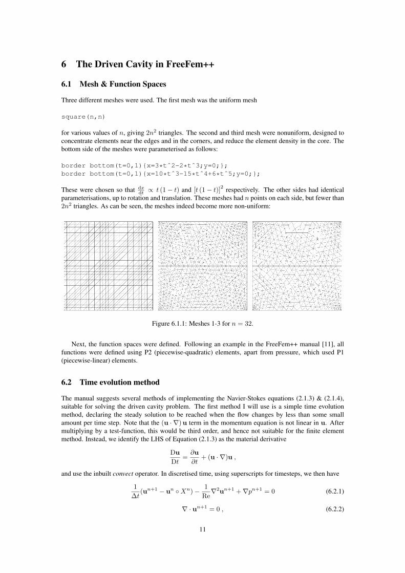
Three different meshes were used. The first mesh was the uniform mesh

square(n,n)

for various values of n, giving 2n2 triangles. The second and third mesh were nonuniform, designed toconcentrate elements near the edges and in the corners, and reduce the element density in the core. Thebottom side of the meshes were parameterised as follows:

border bottom(t=0,1){x=3*tˆ2-2*tˆ3;y=0;};border bottom(t=0,1){x=10*tˆ3-15*tˆ4+6*tˆ5;y=0;};

These were chosen so that dxdt ∝ t (1− t) and [t (1− t)]2 respectively. The other sides had identical

parameterisations, up to rotation and translation. These meshes had n points on each side, but fewer than2n2 triangles. As can be seen, the meshes indeed become more non-uniform:

Figure 6.1.1: Meshes 1-3 for n = 32.

Next, the function spaces were defined. Following an example in the FreeFem++ manual [11], allfunctions were defined using P2 (piecewise-quadratic) elements, apart from pressure, which used P1(piecewise-linear) elements.

6.2 Time evolution method

The manual suggests several methods of implementing the Navier-Stokes equations (2.1.3) & (2.1.4),suitable for solving the driven cavity problem. The first method I will use is a simple time evolutionmethod, declaring the steady solution to be reached when the flow changes by less than some smallamount per time step. Note that the (u · ∇)u term in the momentum equation is not linear in u. Aftermultiplying by a test-function, this would be third order, and hence not suitable for the finite elementmethod. Instead, we identify the LHS of Equation (2.1.3) as the material derivative

Du

Dt=∂u

∂t+ (u · ∇)u ,

and use the inbuilt convect operator. In discretised time, using superscripts for timesteps, we then have

1

∆t(un+1 − un ◦Xn)− 1

Re∇2un+1 +∇pn+1 = 0 (6.2.1)

∇ · un+1 = 0 , (6.2.2)

11

where un ◦Xn represents the convected velocity field,

un ◦Xn ≈ un|x−∆t·un|x .

We take the scalar product of the first equation with a test function v, multiply the second by a testfunction q, and combine the equations. After integration by parts, our analytic problem is: given un, pn,we seek un+1, pn+1 such that ∀v, q,∫

A

(1

∆t

(un+1 · v − (un ◦Xn) .v

)+

1

Re

(∇un+1 : ∇v

)− pn+1∇ · v − q∇ · un+1

)dA = 0 .

(6.2.3)The boundary conditions are simply the velocity boundary conditions on u.

After defining the following macros:

macro Grad(u1,u2) [dx(u1),dy(u1) , dx(u2),dy(u2) ] //macro div(u1,u2) (dx(u1)+dy(u2)) //

to aid readability, as suggested by [11], the time evolution problem is represented by the following code,also taken from [11]:

problem navierst(u1,u2,p,v1,v2,q,init=nsi) =int2d(Th)(alpha*(u1*v1 + u2*v2)

+ nu*(Grad(u1,u2)’*Grad(v1,v2))- 1e-8*p*q- div(u1,u2)*q - div(v1,v2)*p)

+ int2d(Th) (-alpha*convect([up1,up2],-dt,up1)*v1-alpha*convect([up1,up2],-dt,up2)*v2)

+ on(1,2,4,u1=0,u2=0) + on(3,u1=1,u2=0);

where alpha is 1∆t , nu is 1

Re , and u and v have been broken into components u1, u2, v1, v2. Theinit parameter allows the matrices to be reused rather than regenerated each iteration, saving com-putation time. [up1, up2] is the velocity field from the previous timestep, to be used in the convectoperator. A term p · q · 10−8 has been inserted, to aid numerical stability. Finally, the boundary conditionis implemented in the final line, where the labels 1-4 represent the sides of the square.

6.3 Newton iteration method

The second method is a Newton-style iterative procedure. The steady solution has u, p satisfying

(u · ∇)u− ν∇2u +∇p = 0 (6.3.1)

∇ · u = 0 . (6.3.2)

The weak formulation is to find u, p such that ∀v, p,∫A

(((u · ∇)u) · v +

1

Re∇u : ∇v − p∇ · v − q∇ · u

)dA = 0 . (6.3.3)

Newton’s algorithm to solve the generic problem ‘find x in Rn such that F (x) = 0’ is:

1. evaluate the Jacobian DF that satisfies F (x+ δx) = F (x) +DF (x)(δx) + O(δx2)

2. choose some initial x0 ∈ Rn

3. find δxi such that DF (xi)δxi = F (xi), and set xi+1 = xi − δxi

4. repeat 3 until |δxi| is sufficiently small

12

For the steady Navier-Stokes problem, we have

F (u, p) =

∫A

(((u · ∇)u) · v +

1

Re(∇u) : (∇v)− p∇ · v − q∇ · u

)dA (6.3.4)

DF (u, p) (δu, δp) =∫A

(((δu · ∇)u) · v + ((u · ∇) δu) · v +

1

Re∇δu : ∇v − δp∇ · v − q∇ · δu

)dA (6.3.5)

Note that the variables to be solved for are δu and v; u is taken as given in each iteration, therefore weonly have linear and bilinear terms. In FreeFem++ language, this becomes the following, also taken from[11]:

problem NR([du1,du2,dp],[v1,v2,q],init=nri) =int2d(Th)(nu*(Grad(du1,du2)’*Grad(v1,v2))

+ UgradV(du1,du2,u1,u2)’*[v1,v2]+ UgradV(u1,u2,du1,du2)’*[v1,v2]- 1e-8*dp*q- div(du1,du2)*q - div(v1,v2)*dp)

- int2d(Th)(nu*(Grad(u1,u2)’*Grad(v1,v2))+ UgradV(u1,u2,u1,u2)’*[v1,v2]- div(u1,u2)*q - div(v1,v2)*p)

+ on(1,2,3,4,du1=0,du2=0);

where the additional macro

macro UgradV(u1,u2,v1,v2) [ [u1,u2]’*[dx(v1),dy(v1)] ,[u1,u2]’*[dx(v2),dy(v2)] ] //

was used.

Again, a stabilisation term has been used. In addition, the boundary condition imposes δu = 0 on theboundary, i.e. it requires the initial guess to satisfy the correct boundary conditions. While it is plausiblethat if δu 6= 0 is not exactly satisfied, the end solution may no longer satisfy the boundary conditionexactly, in practice this is not an issue, due to the small number of Newton iterations performed. I laterverified this: in the steady solutions obtained, the velocities on the no-slip boundaries were typicallyO(10−20

), as was the vertical velocity on the top plate; the horizontal velocity on the top plate was

exactly 1, since double-precision floating point numbers have some 15 or 16 decimal digits of accuracy.

6.4 Comments

Both the time evolution and Newton iteration methods require some initial velocity and pressure distri-bution. While the flow in the former method may start from rest, this state cannot be used for the lattermethod, since this does not satisfy the boundary conditions of the Driven Cavity problem. In practice, Iwill use parameter continuation extensively, using solutions for similar Re, possibly interpolated from adifferent mesh. Initially, I will use the solution to the Stokes problem with Re = 0, which is identical tothe time-evolution problem with the convect operator removed. Again, the following code is taken from[11]:

problem stokes([u1,u2,p],[v1,v2,q]) =int2d(Th)(Grad(u1,u2)’*Grad(v1,v2)

- 1e-8*p*q- div(u1,u2)*q - div(v1,v2)*p)

+ on(1,2,4,u1=0,u2=0) + on(3,u1=1,u2=0);

13

Finally, it will later be shown that the streamfunction ψ can be used as a proxy for convergence ofother variables, and gives visually intuitive plots. The code used to generate this is again taken from [11]:

problem createsf(psi,phi,init=sfi) =int2d(Th)(dx(psi)*dx(phi) + dy(psi)*dy(phi))+ int2d(Th)(-phi*(dy(u1)-dx(u2)))+ on(1,2,3,4,psi=0);

where we have used a test-function phi, and the relationship

∇2ψ = −ω ,

whereω =

∂uy∂x− ∂ux

∂y,

setting ψ = 0 on the boundary.

Much of the code used is to facilitate file I/O, solution caching, and other things that are less releventto the discussion here, but of great help when running simulations. A full code listing will be given inthe appendix.

7 Results

The following subsections relate to the time evolution method, unless specifically stated otherwise.

7.1 Runtime of individual functions; variation with n, Re, ∆t

The following tests were all carried out using FreeFem++-cs 12.3 running on Windows Vista SP2 (32-bit), with negligible background activity, on a laptop containing an Intel Core 2 Duo T8300 processor.Each test was repeated 3 times, with the median time taken. The maximum deviations were at most 1-2%from the median.

Iterations Time (s)0 0.055

100 0.826200 1.556300 2.270

Table 7.1.1: Re = 10, ∆t = 0.1, mesh 1 (uniform), n = 8. stokes and createsf were executed asingle time, then navierst was executed each iteration.

Iterations Time (s)0 0.053

100 1.365200 2.643300 3.917

Table 7.1.2: Re = 10, ∆t = 0.1, mesh 1 (uniform), n = 8. stokes and createsf were executed asingle time, then navierst and createsf were executed each iteration.

As expected, the results in Tables 7.1.1 and 7.1.2 suggest that execution time scales linearly withthe number of iterations, with some extra time required for the stokes problem and the navierstinitialisation (recall that the internal matrices for navierst are stored to avoid repeated recalculation).

14

In addition, navierst and createsf take comparable time to run, which strongly suggests avoidingmaking calls to createsf every time step.

mesh type n vertices interior vertices triangles Time (s)1 8 81 49 128 3.0151 10 121 81 200 4.5161 12 169 121 288 6.4523 20 224 144 366 8.4681 14 225 169 392 8.7311 16 289 225 512 11.627

Table 7.1.3: Re = 10, ∆t = 0.1, 400 iterations. stokes and createsf were executed a single time,then navierst was executed each iteration.

In Table 7.1.3, we see that for the uniform grids, as expected, execution speed is approximatelyquadratic in n. A non-uniform mesh result has been inserted for comparison. Despite having n = 20,this has almost the same number of total vertices as the uniform mesh with n = 14. It has 14.8% fewerinterior vertices, and 6.6% fewer triangles, but execution time is (only) reduced by 3%, hence executiontime isn’t simply linear in one of these measures.

Re Time (s)10 14.484

100 14.3261000 14.011

Table 7.1.4: ∆t = 0.1, mesh 1 (uniform), n = 32, 100 iterations. stokes and createsf were executeda single time, then navierst was executed each iteration.

In Table 7.1.4, we see that the time taken varies slightly (but consistently) with Re. Note that thisis unrelated to convergence towards a steady flow; we are running a fixed number of iterations. This issomewhat unexpected, but is perhaps related to the iterative methods used in the internal sparse matrixroutines.

∆t Time (s)0.200 17.3680.100 14.3040.050 12.7390.025 12.015

Table 7.1.5: Re = 100, mesh 1 (uniform), n = 32, 100 iterations. stokes and createsf were executeda single time, then navierst was executed each iteration.

In Table 7.1.5, we see that the execution time varies significantly with ∆t, in particular, it seems thatthe execution time goes like t0 +a∆t. To the author, it seems most likely that this behaviour is due to theinbuilt convect function: it is plausible that the timestep ∆t is being broken down into smaller units,and the flow is being convected through each of these smaller time steps (where the size of the smalltime unit is chosen to meet some error tolerance in each small time step). Later results on solution errorswill lend support to this theory.

7.2 ψ as a proxy for convergence

Here, we aim to show that ψ, u and p converge simultaneously, so that it is sufficient to check forconvergence of ψ. The following simulations were done, to cover a range of Re and mesh size, all on auniform mesh:

15

1. n = 8, ∆t = 0.2, Re = 10, 50 steps

2. n = 16, ∆t = 0.1, Re = 100, 200 steps

3. n = 32, ∆t = 0.05, Re = 1000, 800 steps

The main time-step loop was modified by to calculate the differences ∆pn = pn−pn−1, sim. ∆unx , ∆uny ,∆ψn, and output the maximum values ‖∆pn‖∞, etc., to file every iteration. These were then plotted inExcel.

As can be seen in figures 7.2.1-7.2.3, ψ converges at the same rate as u and p. The logs are in fact tobase 10, and in the first picture, we reach the limits of machine precision before step 50 (about 16 decimaldigits; ‖ux‖∞ and ‖uy‖∞ ≈ 1, ‖ψ‖∞ ≈ 0.1, ‖p‖∞ is a few orders of magnitude larger, reflecting thetheoretical singularities in the upper corners.)

Figure 7.2.1: n = 8, ∆t = 0.2, Re = 10

Figure 7.2.2: n = 16, ∆t = 0.1, Re = 100

16

Figure 7.2.3: n = 32, ∆t = 0.05, Re = 1000

7.3 Convergence

Here, we shall investigate how quickly the flow converges to a steady solution, and how this changes with∆t, Re and n.

7.3.1 Dependence on ∆t

The following simulations were all done with n = 32, which is a reasonable mesh to use for obtainingresults (unlike n = 8!) Firstly it was noticed that there were occasions on which ψ would not convergeto an accuracy of 10−16, only to 10−11 or so (for example, the combination Re = 150, ∆t = 0.2 or0.15). Thus, convergence will be deemed to have been reached when ‖∆ψn‖∞ < 10−10. The followingsimulations were done, starting from the solution to the Stokes problem:

1. Re = 25: ∆t = 0.0125, 0.025, 0.05, 0.1, 0.2

2. Re = 100: ∆t = 0.0125, 0.025, 0.05, 0.1, 0.2

3. Re = 400: ∆t = 0.05, 0.07, 0.1, 0.14, 0.2

In all simulations, after initial transients decay, there is a clear regime of exponential decay towardsa steady state. A typical example is shown in figures 7.3.1 and 7.3.2.

17

Figure 7.3.1: ‖∆ψn‖∞/‖∆ψn−1‖∞ against n, for Re = 100; ∆t = 0.0125 (top) to 0.2 (bottom)

Figure 7.3.2: Inside the exponential decay regime: ln(‖∆ψn‖∞) against n, for Re = 100; ∆t = 0.0125(right) to 0.2 (left)

It is natural to plot a log-log graph of the slopes in Figure 7.3.2 (and similar graphs for Re = 25 and400) against ∆t, in this is done in Figures 7.3.3 to 7.3.5.

18

Figure 7.3.3: Re = 25 (∆t = 0.2 omitted due to insufficient time in the exponential decay regime)

Figure 7.3.4: Re = 100

Figure 7.3.5: Re = 400

19

These indeed show that the number of steps needed to converge ∝ 1∆t - but this was clearly to be

expected! This is, of course, consistent with the program modelling the physical flow accurately.

7.3.2 Dependence on Re

The following simulations were done:

1. ∆t = 0.05: Re = 25, 50, 100, 200, 400

2. ∆t = 0.1: Re = 25, 50, 100, 200, 400

3. ∆t = 0.2: Re = 25, 50, 100, 200, 400

Again, log-log graphs were plotted of slope against Re.

Figure 7.3.6: ∆t = 0.05

Figure 7.3.7: ∆t = 0.1

20

Figure 7.3.8: ∆t = 0.2

The relationship in Figures 7.3.6-7.3.8 is less clear-cut. The number of steps needed to convergeunsurprisingly increases with Re, but doesn’t seem to follow a simple power law. In the Re = 25 to Re= 400 regime, the number of steps ∝ Re0.775 or so, as a first approximation, but the deviations from astraight line on the log-log plots are consistent for the different ∆t’s.

7.3.3 Dependence on n

The following simulations were done:

1. Re = 10, ∆t = 0.1: n = 16, 23, 32, 45, 64

2. Re = 100, ∆t = 0.1: n = 16, 23, 32, 45, 64

n steps16 2923 2732 2645 2764 28

Table 7.3.1: Re = 10, ∆t = 0.1: steps taken to converge, starting from the Stokes solution

n steps16 26723 26832 26845 26864 268

Table 7.3.2: Re = 100, ∆t = 0.1: steps taken to converge, starting from the Stokes solution

As can be seen from tables 7.3.1 and 7.3.2, the number of steps needed to converge is (essentially)independent of the mesh used. This increases our confidence that we are indeed modelling the physicalflow somewhat accurately.

7.4 Elementary failures of convergence

We expect that our problem will fail to converge at sufficiently large Re. We will investigate this briefly.

21

Re Result400 converges to steady800 converges to steady

1500 converges to steady1600 oscillates, fails to converge3200 converges to a spurious double-loop solution6400 spurious double loop (seemingly unsteady)

10000 spurious double loop (unsteady)20000 spurious double loop (almost nonsense)40000 nonsense

Table 7.4.1: n = 8, ∆t = 0.2

Re Result1500 converges to steady1600 converges to steady1800 converges to steady1850 converges to steady1875 spurious double loop1900 spurious double loop2000 spurious double loop

Table 7.4.2: n = 8, ∆t = 0.1

Re Result1600 converges to steady3200 converges to steady6400 converges to steady8000 converges to steady9000 spurious double loop

Table 7.4.3: n = 16, ∆t = 0.2

The above results show that convergence can be achieved at higher Re by decreasing ∆t, but mainlyby increasing n.

Typical streamfunction plots of the steady, double-loop and nonsense states are shown in figures7.4.1-7.4.3. The isovalues plotted are not evenly spaced, and are instead chosen to emphasise the non-primary vortices. It is interesting to see that we obtain the same spurious double-loop solution as thoseseen in the literature, as mentioned previously, and alluded to in [6].

22

Figure 7.4.1: n = 8, ∆t = 0.2, Re = 400, steady solution

Figure 7.4.2: n = 8, ∆t = 0.2, Re = 3200, steady spurious double loop

Figure 7.4.3: n = 8, ∆t = 0.2, Re = 40000, very unsteady solution (though slightly coherent)

23

7.5 Steady solutions with the time-evolution method

As a side-effect of running the previous simulations, it became clear that the results were not independentof ∆t and n, even though the streamline plots were superficially similar. From this point onwards, weshall restrict our attention to the flow variable ψmax, which corresponds to the value of ψ at the centre ofthe primary vortex, typically≈ 0.1. This is used throughout the literature in comparisons between papers(in papers where the lid moves from right to left, this becomes ψmin - needless to say the conversion istrivial).

7.5.1 Dependence on ∆t

The following simulations were run, for n = 16:

1. Re = 25: ∆t = 0.4, 0.28, 0.2, 0.14, 0.1, 0.07, 0.05, 0.035, 0.025, 0.0175, 0.0125, 0.01

2. Re = 100: ∆t = 0.4, 0.28, 0.2, 0.14, 0.1, 0.07, 0.05, 0.035, 0.025, 0.0175, 0.0125, 0.01

3. Re = 400: ∆t = 0.4, 0.28, 0.2, 0.14, 0.1, 0.07, 0.05, 0.035, 0.025, 0.0175, 0.0125, 0.01

Results are in Table 7.5.1; this is plotted in Figure 7.5.1.

ψmax

∆t Re = 25 Re = 100 Re = 4000.4 0.0938137 0.0853667 0.070120.28 0.0951156 0.0883954 0.0746310.2 0.0960474 0.0908261 0.0788390.14 0.0967591 0.0928685 0.08297830.1 0.0972329 0.0943222 0.08616880.07 0.0975783 0.0955438 0.0892810.05 0.0977932 0.0963963 0.09163760.035 0.097945 0.0969928 0.09353770.025 0.0980452 0.0974017 0.09482520.0175 0.0981256 0.0977299 0.09564180.0125 0.0981776 0.0979501 0.09626990.01 0.0982043 0.0980684 0.0966181

Table 7.5.1: Dependence on ∆t: Re = 25, 100, 400; n = 16

24

Figure 7.5.1: ψmax against ∆t, n = 16

The above plot strongly suggests that the leading-order error term is O (∆t). This is in agreementwith my earlier hypothesis about the convect operator: that the timestep ∆t is broken down intosmaller timesteps, such that the error during each small timestep is smaller than some tolerance - leadingto the total error being linear in ∆t.

7.5.2 Dependence on n

The following simulations were run, for Re = 100:

1. ∆t = 0.1: n = 8, 11, 16, 23, 32, 45, 64

2. ∆t = 0.05: n = 8, 11, 16, 23, 32, 45, 64

3. ∆t = 0.025: n = 8, 11, 16, 23, 32, 45, 64

Results are in Table 7.5.2; this is plotted in Figure 7.5.2.

ψmax

n ∆t = 0.1 ∆t = 0.05 ∆t = 0.0258 0.0899634 0.0914896 0.092337411 0.0922175 0.093955 0.094848216 0.0943222 0.0963963 0.097401723 0.0954286 0.0977388 0.098872932 0.0960135 0.0984644 0.099738645 0.0963704 0.0990315 0.10040364 0.0965907 0.0993701 0.100855

Table 7.5.2: Dependence on n: ∆t = 0.1, 0.05, 0.025; Re = 100

25

Figure 7.5.2: ψmax against n−1, Re = 100

The above plot suggests that the leading-order error term is O(

1n

), but this is not completely clear,

especially for ∆t = 0.1.

7.5.3 Repeated extrapolation

We have seen that naive extrapolation in n may be of questionable use. It seems to reasonable to attemptextrapolation in ∆t, then extrapolation in n: the former giving a ‘perfect’ solution for a given mesh, thelatter removing the mesh dependence.

For Re = 10, 100, we will linearly extrapolate the results for ∆t = 0.05 and 0.025 to give a result for∆t = 0, and see how this varies with n, for n = 16, 19, 23, 27, 32, 38, 45, 54, 64, 76, 91.

Results are given in Tables 7.5.3 and 7.5.4, and the extrapolated values are plotted in Figure 7.5.3.

ψmax

n ∆t = 0.05 ∆t = 0.025 ∆t = 0 (Extr)16 0.0980122 0.0981159 0.098219619 0.0985264 0.0986324 0.098738423 0.0987878 0.0988976 0.099007427 0.0989469 0.0990607 0.099174532 0.0991109 0.0992281 0.099345338 0.0992271 0.0993484 0.099469745 0.0993098 0.0994345 0.099559254 0.099394 0.099523 0.09965264 0.0994797 0.0996122 0.099744776 0.09953 0.0996659 0.099801891 0.0995841 0.099723 0.0998619

Table 7.5.3: Re = 10: dependence of extrapolated result on n

26

ψmax

n ∆t = 0.05 ∆t = 0.025 ∆t = 0 (Extr)16 0.0963963 0.0974017 0.098407119 0.097095 0.0981454 0.099195823 0.0977388 0.0988729 0.10000727 0.0981572 0.0993668 0.100576432 0.0984644 0.0997386 0.101012838 0.0987623 0.100107 0.101451745 0.0990315 0.100403 0.101774554 0.0992281 0.100669 0.102109964 0.0993701 0.100855 0.102339976 0.0994811 0.101009 0.102536991 0.0995733 0.101145 0.1027167

Table 7.5.4: Re = 100: dependence of extrapolated result on n

Figure 7.5.3: ψmax against n−1, Re = 10 and 100

Linear extrapolation in n now seems more justified. This gives a modus operandi: for a given Re,

1. For a given n, obtain a converged solution at two small values of ∆t

2. For this n, use the above results to extrapolate a solution for ∆t = 0

3. Use the results at several values of n to extrapolate a result as n−1 → 0

7.6 Comparison with literature

We use ∆t = 0.035 and 0.025, n = 45 and 64.

27

ψmax

n ∆t = 0.035 ∆t = 0.025 ∆t = 0 (Extr)45 0.0998591 0.100403 0.10176364 0.100258 0.100855 0.102348

Result: 0.103732Ghia, Ghia & Shin ’82 [4]: 0.103423

Table 7.6.1: Re = 100

ψmax

n ∆t = 0.035 ∆t = 0.025 ∆t = 0 (Extr)45 0.101282 0.10317 0.1078964 0.102364 0.104456 0.109686

Result: 0.11394Ghia, Ghia & Shin ’82 [4]: 0.113909

Table 7.6.2: Re = 400

ψmax

n ∆t = 0.035 ∆t = 0.025 ∆t = 0 (Extr)45 0.0974772 0.100418 0.1077764 0.0989792 0.102308 0.11063

Result: 0.117404Erturk, Corke & Gokcol ’05 [8]: 0.118942

Barragy & Carey ’97 [7]: 0.118930Schreiber & Keller ’83 [5]: 0.11894Benjamin & Denny ’79 [3]: 0.1193

(Ghia, Ghia & Shin ’82 [4]:) (0.117929)

Table 7.6.3: Re = 1000 - note the result from Ghia et. al. is somewhat different to the others

ψmax

n ∆t = 0.035 ∆t = 0.025 ∆t = 0 (Extr)45 0.0890742 0.0929585 0.10266964 0.0909806 0.0954064 0.106471

Result: 0.115475Erturk, Corke & Gokcol ’05 [8]: 0.121470

Table 7.6.4: Re = 2500 - the extrapolated result is now way off

The results for Re = 100 and 400 seem promising, although the results available in the literature arelimited. By Re = 1000, while results in the literature cluster around 0.1189, the extrapolated result is only0.1174, and the gap widens even more for Re = 2500. We must be able to do better...

7.7 Non-uniform meshes

Everything up to now has used the uniform mesh within a square. We now introduce the custom non-uniform meshes. One downside is that we cannot expect to get useful results by extrapolation in n, dueto the non-uniformity of the meshes, but we can still extrapolate in ∆t. Results are given below, in tables7.7.1-7.7.4.

28

ψmax

n ∆t Mesh 1 Mesh 2 Mesh 332 0.035 0.099233 0.101296 0.101554

0.025 0.0997386 0.101824 0.1020770 (Extrap) 0.101002 0.103144 0.103385

45 0.035 0.0998591 0.101393 0.1015580.025 0.100403 0.101951 0.1020920 (Extrap) 0.101763 0.103346 0.103427

64 0.035 0.100258 0.101409 0.1015210.025 0.100855 0.101996 0.1020830 (Extrap) 0.102348 0.103464 0.103488

Previous result: 0.103732Ghia, Ghia & Shin ’82 [4]: 0.103423

Table 7.7.1: Re = 100

ψmax

n ∆t Mesh 1 Mesh 2 Mesh 332 0.035 0.099616 0.105359 0.106320

0.025 0.101374 0.107347 0.1083140 (Extrap) 0.105770 0.112317 0.113299

45 0.035 0.101282 0.105701 0.1062560.025 0.103170 0.107802 0.1083200 (Extrap) 0.107890 0.113055 0.113480

64 0.035 0.102364 0.105720 0.1060960.025 0.104456 0.107862 0.1082100 (Extrap) 0.109686 0.113217 0.113495

Previous result: 0.113940Ghia, Ghia & Shin ’82 [4]: 0.113909

Table 7.7.2: Re = 400

ψmax

n ∆t Mesh 1 Mesh 2 Mesh 332 0.035 0.095061 0.103895 0.105330

0.025 0.097759 0.106935 0.1086920 (Extrap) 0.104504 0.114535 0.117097

45 0.035 0.097477 0.104151 0.1051940.025 0.100418 0.107607 0.1087400 (Extrap) 0.107770 0.116247 0.117605

64 0.035 0.098979 0.104064 0.1046190.025 0.102308 0.107584 0.1081300 (Extrap) 0.110630 0.116384 0.116908

Previous result: 0.117404Erturk, Corke & Gokcol ’05 [8]: 0.118942

Table 7.7.3: Re = 1000

29

ψmax

n ∆t Mesh 1 Mesh 2 Mesh 332 0.035 0.086160 0.097610 0.101349

0.025 0.089171 0.101193 0.1065560 (Extrap) 0.096699 0.110150 0.119574

45 0.035 0.089074 0.098326 0.0996340.025 0.092959 0.103111 0.1047570 (Extrap) 0.102669 0.115074 0.117565

64 0.035 0.090981 0.098019 0.0989970.025 0.095406 0.102901 0.1039610 (Extrap) 0.106471 0.115107 0.116371

Previous result: 0.115475Erturk, Corke & Gokcol ’05 [8]: 0.121470

Table 7.7.4: Re = 2500

Clearly the individual results are far more accurate on the non-uniform meshes. The results on Mesh3, with n = 32 and ∆t = 0.035 are more accurate than the results on the uniform mesh with n = 64and ∆t = 0.025 for all four values of Re (now is a good time to recall the past finding that simulationson Meshes 2 and 3 are faster than on Mesh 1 at the same n). Unfortunately, we give up a lot by notbeing able to extrapolate in n−1 (indeed, some of the results above aren’t even monotonic in n), and thedoubly-extrapolated Mesh 1 results are generally better than the singly-extrapolated Mesh 2 and Mesh 3results.

7.8 The Newton method

As has been shown, the IVP formulation could be made to give reasonably accurate results. However, theexecution speed was far from optimal, and the simulations at Re = 2500 on the finest meshes were takingseveral hours (parameter continuation did not reduce this much, since the solution changed by 10−3 to10−2 when ∆t, n or Re were changed, while we demanded convergence to 10−10).

The Newton method executes much more quickly. However, it is unlikely to converge unless theinitial flow is somewhat close to the steady flow, so parameter continuation will be used extensively. Atypical set of results is given below, in Table 7.8.1. These are plotted in Figure 7.8.1.

ψmax

n Mesh 1 Mesh 2 Mesh 3 Comment32 0.105417 0.116718 0.118166 initialised with time evolution solution with ∆t = 0.02545 0.109077 0.117812 0.118725 initialised with time evolution solution with ∆t = 0.02564 0.111891 0.118365 0.118819 initialised with time evolution solution with ∆t = 0.02591 0.111372 0.118350 0.118864 initialised with Newton-64 solution128 0.111377 0.118377 0.118881 initialised with Newton-91 solution

Previous result: 0.117404Erturk, Corke & Gokcol ’05 [8]: 0.118942

Table 7.8.1: Re = 1000

30

Figure 7.8.1: ψmax against n−1, Re = 1000, Newton Method

A typical result is shown in Table 7.8.1. Although it is not immediately obvious that something iswrong, Figure 7.8.1 suggests that there is a problem. It seems that the solutions obtained at n = 91,128 are spurious. This was not obvious, since the streamline plots were almost identical to the genuinesolution. Note that these were continued from other Newton results, while the ones continued from theIVP were fine. The accuracy of the genuine solutions should be emphasised, though. At n = 64, on Mesh3, we are a mere 10−4 away from the answers given in the literature, and the Newton convergence tookwell under a minute. However, we did begin with the result of an IVP simulation that took several hours.

7.9 A New(ton) Hope?

The findings from the previous section suggest a unified method: one that uses the incredibly fast conver-gence of the Newton method, with occasional time evolution steps to ensure we are on the right solutionbranch. While the method I settled on is far from perfect, it seemed to work: Given an initial guess forthe steady flow,

1. Carry out a small number of time evolution steps.

2. Carry out Newton iterations. If convergence does not occur, reload time evolution results, reducetime step but increase number of steps.

3. Repeat 1 and 2 until two consecutive Newton procedures converge, and to the same result.

It is certainly feasible that we may converge to the same spurious solution twice. However, it was foundthat we indeed converged to the same flow as the solutions above that were initialised with a time evolu-tion steady state, but to a slightly different flow to the solutions generated above that were initialised bya Newton method solution.

Using this method, steady solutions were generated on Mesh 3 with n = 128, 160, 192. Steadysolutions were generated for Re = 100 to 5000 in steps of 100, and beyond Re = 5000 in steps of 500.Each attempt was initialised with the steady solution of the previous Re, with Re = 100 initialised withthe Stokes solution. At the largest few values of Re (for each n), steps of 500 were insufficient to preventblowup, and steps of 100 were used. In addition, the timestep ∆t was decreased from 0.1 to as little as0.001. Results will be listed below, with comparisons made to extrapolated results in Erturk et. al. [8] andBarragy & Carey [7] where appropriate. Later simulations with n = 193 and 200 were also done, theseresults are also included below.

31

ψmax

Re n = 128 n = 160 n = 192 n = 193 n = 200 Erturk [8] Barragy [7]500 0.115411 0.115414 0.115420 0.115419 0.115419

1000 0.118923 0.118929 0.118932 0.118933 0.118934 0.118942 0.1189301500 0.120320 0.120321 0.120327 0.120329 0.1203292000 0.121036 0.121042 0.121043 0.121046 0.1210452500 0.121460 0.121461 0.121464 0.121463 0.121463 0.121470 0.1214623000 0.121726 0.121732 0.121734 0.121735 0.1217353500 0.121919 0.121917 0.121919 0.121919 0.1219214000 0.122056 0.122055 0.122050 0.122054 0.1220514500 0.122163 0.122156 0.122149 0.122151 0.1221485000 0.122244 0.122231 0.122222 0.122224 0.122221 0.122233 0.1222197500 0.122425 0.122408 0.122388 0.122390 0.122384 0.122386 0.122380

10000 0.122474 0.122446 0.122408 0.122418 0.122404 0.122390 0.12239312500 0.122497 0.122446 0.122384 0.122403 0.122379 0.122326 0.12235815000 0.122499 0.122436 0.122343 0.122374 0.122338 0.12224517500 0.122477 0.122426 0.122299 0.122335 0.122291 0.122167 -20000 0.122445 0.122416 0.122257 0.122292 0.122242 0.122084 -

(21000) 0.122434 0.122411 0.122242 0.122275 0.122223 0.122056 -22500 0.122423 0.122404 0.122223 0.122249 0.122196 - -25000 0.122420 0.122391 0.122198 0.122210 0.122155 - -27500 0.122441 0.122374 0.122175 0.122173 0.122121 - -30000 0.122474 0.122356 0.122143 0.122139 0.122092 - -32500 0.122470 0.122343 0.122094 0.122105 0.122069 - -35000 0.122312 0.122346 0.122016 0.122069 0.122048 - -

(37200) 0.122392 - -37500 - 0.122381 0.121907 0.122031 0.122030 - -40000 - 0.122458 0.121773 0.121994 0.122013 - -42500 - 0.122578 0.121625 0.121958 0.121995 - -45000 - 0.122746 0.121469 0.121922 0.121976 - -

(47300) - 0.121961 - -47500 - 0.122977 0.121303 0.121896 - - -

(48600) - 0.121887 - - -50000 - 0.123296 0.121146 - - - -52500 - 0.123915 0.120986 - - - -

(53900) - 0.124354 - - - -55000 - - 0.120840 - - - -57500 - - 0.120712 - - - -60000 - - 0.120609 - - - -62500 - - 0.120555 - - - -

(63600) - - 0.120542 - - - -

Table 7.9.1: Results with unified method (‘-’ indicates a failure to reach a steady solution; a blank cellindicates that a steady solution was reached for some higher Re, but no simulation was done at this Re.In particular, Barragy and Carey obtained a solution at Re = 16,000, but did not publish their ψmax)

Several plots of streamfunctions of steady flows generated by the above method follow. Isovalues willbe plotted at -0.03, -0.02, -0.01, -3×10−3, -10−3, ..., -3×10−8, -10−8, -10−9, 0, 10−9, 10−8, 3×10−8,..., 10−3, 3×10−3, 0.01, 0.02, ..., 0.10, 0.11, 0.12 so that the weak corner vortices may be clearly seen.

Finally, two figures will be shown of the computed ux and uy velocities along lines through thegeometric centre of the cavity.

32

Figure 7.9.1: Mesh 3, n = 192. To be used in the plots below.

Figure 7.9.2: Re = 0, solution of the Stokes problem. Note the left-right symmetry. Secondary vorticesin the bottom corners are visible.

33

Figure 7.9.3: Unified method, Re = 100. The primary vortex centre has been shifted downstream and isslightly lower. The bottom-right secondary vortex has grown, the bottom-left vortex has shrunk slightly.

Figure 7.9.4: Unified method, Re = 400. The primary vortex centre approaches the centre of the cavity.The secondary vortices have grown, and a tertiary vortex in the bottom-right is just visible.

34

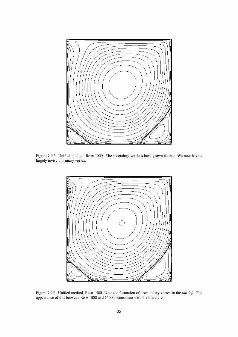
Figure 7.9.5: Unified method, Re = 1000. The secondary vortices have grown further. We now have alargely inviscid primary vortex.

Figure 7.9.6: Unified method, Re = 1500. Note the formation of a secondary vortex in the top-left. Theappearance of this between Re = 1000 and 1500 is consistent with the literature.

35

Figure 7.9.7: Unified method, Re = 2500. The secondary vortex in the top-left and its impact on the floware now obvious. Tertiary vortices in both bottom corners are just visible.

Figure 7.9.8: Unified method, Re = 10000. Tertiary vortices in the bottom corners are clearly formed.

36

Figure 7.9.9: Unified method, Re = 15000. A tertiary vortex in the top-left can be identified.

Figure 7.9.10: Unified method, Re = 30000. A fourth-order vortex can be clearly seen in the bottom-rightcorner; a fourth-order vortex in the bottom-left may also be visible.

37

Figure 7.9.11: Unified method, Re = 50000. The fourth-order vortex in the bottom-left is more visible.

Figure 7.9.12: Unified method, Re = 63600. Both fourth-order vortices are clearly visible. In the up-per left corner, a second tertiary vortex may have formed below the first tertiary vortex (compare thesecondary vortex at c. 1500, and the first tertiary vortex at c. 10000).

38

Figure 7.9.13: Unified method, ux velocities along the line x = 0.5, for several values of Re. These arein agreement with results in the literature, specifically those in [8]. The non-monotinicity near the lid isnot an artifact.

Figure 7.9.14: Unified method, uy velocities along the line y = 0.5, for several values of Re. Note thelargely inviscid core in the above diagrams, for Re ≥ 1000.

39

8 Conclusion

The results with the unified method show that FreeFem++ is very capable. The author believes that theseare the first qualitatively correct, converged, steady solutions that have been found for Re > 21,000.In particular, the author believes that the second tertiary vortex seen forming in the Re = 63,600 plothas not been seen in the literature before. While Nallasamy and Prasad [19] presented results up to Re= 50,000, their ψmax for Re = 1,000 was some 20% below the 0.1189 common in the literature, andtheir streamfunction contours for Re = 30,000 resemble ‘rounded squares’ and give no indication of therich counter-rotating vortex structure seen here and elsewhere in the literature, thus their results can bediscounted. Erturk et. al. write “Nallasamy and Prasad have presented steady solutions for Reynoldsnumbers up to Re≤ 50000, however, their solutions are believed to be inaccurate as a result of excessivenumerical dissipation caused by their first order upwind difference scheme.”

The n = 192, 193, 200 results tabulated above are in perfect agreement with the existing literatureuntil at least Re = 7,500. However, the variation with n is very interesting. While there is a general trendbetween n = 128, 160 and 192, the difference between results at the same Re for n = 192 and n = 193suggest that there is some ‘randomness’ that depends on the exact triangulation used. In addition, I wasable to obtain converged results beyond Re = 50,000 for n = 160 and 192, but not for n = 193 and 200!There is a sufficiently large difference between the results obtained for different n (and sufficiently littleexisting literature) that I only claim the solutions at very high Re are qualitatively correct. Beyond Re =10,000 or so, the difference between the n = 192, 193, 200 solutions suggest that these are fundamen-tally different (although visually similar) solutions. Though one might be tempted to put this down tobifurcations, repeated attempts to reach a different solution ‘branch’ for Re ≤ 30,000 for n = 128 werecompletely unsuccessful. Vorticity plots at high Re (not shown) suggest the solutions are underresolvedfor Re & 5,000.

One thing that should be emphasised is the simplicity of the algorithms used here. In particular, bothalgorithms were taken from the FreeFem++ manual, and once the time-evolution convergence results hadbeen seen, it became an obvious to use the Newton method to speed up the ‘slow’ transient decay. Thiswas even more of a no-brainer when the lack of independence of the steady solution on the timestep ∆twas noticed. An obvious thing that was not investigated in this essay was the use of the adaptmeshfunction to generate a non-uniform mesh. This was briefly tested: due to the singularities, the uppercorners were given an incredibly high density of elements, while the lower corners were much moresparesly populated. It is unlikely that the fourth-order vortices would have been identified, due to the lowmesh density in these corners. In addition, it was relatively hard to control the number of triangles inthe mesh produced: this had to be done through trial-and-error by setting a tolerance parameter. Thereis a command to limit the number of triangles produced, but this seemed to simply halt the triangulationalgorithm prematurely, rather than giving an optimal mesh. Due to time constraints, this was thereforedropped.

The non-uniform meshes lacked the desireable property of being able to meaningfully extrapolateresults in n, and in addition, the lack of structure in the mesh led to some degree of ‘randomness’ as seenabove. Barragy and Carey [7] used a ‘stretched grid’ with predictable structure; perhaps that would haveled to better results. Finally, FreeFem++ refused to run the algorithms on overly dense meshes: I hadplanned to use the unified method on larger n, say n = 256, but I was unable to go beyond n = 200. Thiswas perhaps due to numerical tolerance issues. Nevertheless, this was slightly disappointing. Executiontime was barely an issue, even for n = 200, each solution took a minute or two, and solutions in intervalsof 500 up to Re = 50,000 could be generated in a few hours.

A Directory Structure and Code Listings

The files should all be placed in the same directory. The subdirectory /cache/ is used to store bothincomplete and complete calculations, described in further detail below. Filenames are of the formmesh-n-Re-dt-variable.txt, where mesh is the mesh type 1, 2 or 3, and the parameter dtis ∆t for an IVP solution, 0 for a Newton solution, and -1 for a Unified solution. variable is velou,

40

velov, sfunc, vorti or press, for the velocity components, pressure, streamfunction and vorticityrespectively. The subdirectory /mesh/ is used to store the meshes. The subdirectory /output/ is usedto store log-style output, including variables like ψmax. The main file is CavFunc.idp. This containsa single function Cavity, which aims to find a steady solution using a particular method, for a givenRe, for a given timestep, on a given mesh, starting from a specified initial state. It is intended that thisis called via CavWrap.edp, either using the parameters listed within that file, or as a loop, to facilitatebatch runs.

The caching system should be briefly explained: the function in CavFunc.idp takes boolean pa-rameters toload and tosave, and a set of loading parameters, corresponding to a particular solutionto load. If toload is set to false, the loading parameters will be ignored and a Stokes solution will begenerated before timesteps or Newton iterations are carried out. If toload is set to true, the /cache/subdirectory will firstly be examined for velocity and pressure files corresponding to the current simu-lation. If velocity and pressure files corresponding to the current simulation exist, these will be loaded,and timesteps or Newton iterations will begin (if the loaded solution corresponds to the converged steadystate then the timesteps/Newton iterations will soon terminate). If the files corresponding to the currentsimulation do not exist, velocity and pressure files corresponding to the loading parameters will be used(if these do not exist, an exception will be thrown, and FreeFem++ will crash). If tosave is set totrue, velocity, pressure, vorticity and streamfunction files will be saved when a converged solution isreached (all methods), and for the time evolution method only, every 100 timesteps. The streamfunctionand vorticity variables are considered derived quantities, and hence only the velocity and pressure filesare used when loading. The streamfunction and vorticity may of course be plotted.

Code listings follow:

meshgen.edp

/* This program is used to generate the meshes */for (int n=8;n<=32;n++) // or whatever{

mesh Ah, Bh, Ch;

Ah=square(n,n);

border C1(t=0,1){x=3*tˆ2-2*tˆ3;y=0;label=1;};border C2(t=0,1){x=1;y=3*tˆ2-2*tˆ3;label=2;};border C3(t=1,0){x=3*tˆ2-2*tˆ3;y=1;label=3;};border C4(t=1,0){x=0;y=3*tˆ2-2*tˆ3;label=4;};Bh = buildmesh(C1(n)+C2(n)+C3(n)+C4(n));

border D1(t=0,1){x=10*tˆ3-15*tˆ4+6*tˆ5;y=0;label=1;};border D2(t=0,1){x=1;y=10*tˆ3-15*tˆ4+6*tˆ5;label=2;};border D3(t=1,0){x=10*tˆ3-15*tˆ4+6*tˆ5;y=1;label=3;};border D4(t=1,0){x=0;y=10*tˆ3-15*tˆ4+6*tˆ5;label=4;};Ch = buildmesh(D1(n)+D2(n)+D3(n)+D4(n));

//plot(Ah,grey=1);//plot(Bh,grey=1);//plot(Ch,grey=1);savemesh(Ah,"mesh\\1-"+n+"-mesh.msh");savemesh(Bh,"mesh\\2-"+n+"-mesh.msh");savemesh(Ch,"mesh\\3-"+n+"-mesh.msh");

}

41

load.idp

/* Loads velocity components and pressure from files */

// Should really put { } around the whole thing, but only called onceint fileexist = 1;// If file doesn’t exist, exception is thrown; fileexist set to 0try {

ifstream f1("cache\\"+meshtype+"-"+n+"-"+re+"-"+qdt+"-velou.txt");} catch (...) fileexist = 0;

if (fileexist) {ifstream f1("cache\\"+meshtype+"-"+n+"-"+re+"-"+qdt+"-velou.txt");ifstream f2("cache\\"+meshtype+"-"+n+"-"+re+"-"+qdt+"-velov.txt");ifstream f3("cache\\"+meshtype+"-"+n+"-"+re+"-"+qdt+"-press.txt");f1 >> u1[]; f2 >> u2[]; f3 >> p[];

} else {ifstream f1("cache\\"+ltype+"-"+ln+"-"+lre+"-"+ldt+"-velou.txt");ifstream f2("cache\\"+ltype+"-"+ln+"-"+lre+"-"+ldt+"-velov.txt");ifstream f3("cache\\"+ltype+"-"+ln+"-"+lre+"-"+ldt+"-press.txt");// if we are on a different mesh, convert to new meshif ((meshtype != ltype) || (n != ln)) {

mesh ThA = readmesh("mesh\\"+ltype+"-"+ln+"-mesh.msh");fespace XhA(ThA,P2);fespace MhA(ThA,P1);XhA u1A, u2A;MhA pA;f1 >> u1A[]; f2 >> u2A[]; f3 >> pA[];u1 = u1A; u2 = u2A; p = pA; // convert

} else {f1 >> u1[]; f2 >> u2[]; f3 >> p[];

}}

save.idp

/* Saves velocity, pressure and streamfunction to file */

ofstream f1("cache\\"+meshtype+"-"+n+"-"+re+"-"+qdt+"-velou.txt");ofstream f2("cache\\"+meshtype+"-"+n+"-"+re+"-"+qdt+"-velov.txt");ofstream f3("cache\\"+meshtype+"-"+n+"-"+re+"-"+qdt+"-press.txt");ofstream f4("cache\\"+meshtype+"-"+n+"-"+re+"-"+qdt+"-sfunc.txt");ofstream f5("cache\\"+meshtype+"-"+n+"-"+re+"-"+qdt+"-vorti.txt");

f1 << u1[]; f2 << u2[]; f3 << p[]; f4 << psi[]; f5 << w[];

42

problems.idp

macro Grad(u1,u2) [dx(u1),dy(u1) , dx(u2),dy(u2) ] //macro UgradV(u1,u2,v1,v2) [ [u1,u2]’*[dx(v1),dy(v1)] ,

[u1,u2]’*[dx(v2),dy(v2)] ] //macro div(u1,u2) (dx(u1)+dy(u2)) //

problem createsf(psi,phi,init=sfi) =int2d(Th)(dx(psi)*dx(phi) + dy(psi)*dy(phi))+ int2d(Th)(-phi*(dy(u1)-dx(u2)))+ on(1,2,3,4,psi=0);

problem stokes([u1,u2,p],[v1,v2,q]) =int2d(Th)(Grad(u1,u2)’*Grad(v1,v2)

- 1e-8*p*q- div(u1,u2)*q - div(v1,v2)*p)

+ on(1,2,4,u1=0,u2=0) + on(3,u1=1,u2=0);

problem navierst(u1,u2,p,v1,v2,q,init=nsi) =int2d(Th)(alpha*(u1*v1 + u2*v2)

+ nu*(Grad(u1,u2)’*Grad(v1,v2))- 1e-8*p*q- div(u1,u2)*q - div(v1,v2)*p)

+ int2d(Th) (-alpha*convect([up1,up2],-dt,up1)*v1-alpha*convect([up1,up2],-dt,up2)*v2)

+ on(1,2,4,u1=0,u2=0) + on(3,u1=1,u2=0);

problem NR([du1,du2,dp],[v1,v2,q],init=nri) =int2d(Th)(nu*(Grad(du1,du2)’*Grad(v1,v2))

+ UgradV(du1,du2,u1,u2)’*[v1,v2]+ UgradV(u1,u2,du1,du2)’*[v1,v2]- 1e-8*dp*q- div(du1,du2)*q - div(v1,v2)*dp)

- int2d(Th)(nu*(Grad(u1,u2)’*Grad(v1,v2))+ UgradV(u1,u2,u1,u2)’*[v1,v2]- div(u1,u2)*q - div(v1,v2)*p)

+ on(1,2,3,4,du1=0,du2=0);

43

CavFunc.idp

func int Cavity(int method, int n, int meshtype, real re, real delt,real tol, int IVPminsteps, int IVPmaxsteps, bool toload,int ln,

int ltype, real lre, real ldt, bool tosave, bool intplot, bool ep)

/* Method 1 is IVP, Method 2 is Newton, Method 3 is combined */{/* DECLARE MESH */mesh Th;

/* INITIALISE MESH */Th = readmesh("mesh\\"+meshtype+"-"+n+"-mesh.msh");if (intplot) plot(Th,cmm="Mesh "+meshtype+", n="+n);

/* DECLARE FUNCTION SPACES ON MESH */fespace Xh(Th,P2);fespace Mh(Th,P1);

/* DECLARE FUNCTIONS */Xh u1, u2, psi, w; // velocity, streamfunction, vorticityXh v1, v2, phi; // test-functions for Finite Elements

Xh psip, psid; // previous value psi_prev, psi_diffMh p, q; // pressure and pressure test-functionXh up1, up2; // previous values, for convectXh du1, du2; // du for Newton methodsMh dp; // dp for Newton methodsXh psipp; // store a Newton-converged psiMh pp; // store p, in case Newton blows up

/* CONSTANT DECLARATION */real dt = delt; // gets changed in method 3

real nu = 1/re;real alpha;int sfi=0, nsi=0, nri=0; // init variables

int jj = 0; // related to init for method 3real qdt = delt; // for loading file purposesif (method==2) qdt = 0; // Newton files have dt = 0 (hack)if (method==3) qdt = -1; // Unified files have dt = -1 (hack)

/* PROBLEM DEFINITIONS */include "problems.idp"

/* INITIALISE FUNCTIONS (VELOCITY, PRESSURE) */if (toload) {include "load.idp" // load stored velocity/pressure} else stokes; // otherwise start from Stokes solution

createsf; sfi=1; // create streamfunctionif (intplot) plot(psi,cmm="Re="+re+" start");

/* OPEN OUTPUT FILE FOR WRITING */ofstream ofile("output\\output.txt",append);ofile << "method="<<method<<", mesh="<<meshtype<<

", n="<<n<<", Re="<<re<<", dt="<<dt<<endl;

44

if (method==1) {alpha = 1/dt;/* MAIN TIME-STEP LOOP */for(nsi=0;nsi<IVPmaxsteps;nsi++) {

up1 = u1; up2 = u2;navierst;

// every IVPminsteps, check for convergenceif(!(nsi%IVPminsteps) && nsi) {

psip = psi;createsf;if (intplot) plot(psi,cmm="Re="+re+", "+nsi+" steps");psid = psi-psip;ofile<<nsi<<" "<<psid[].linfty<<" "<<psi[].linfty<<endl;if (psid[].linfty < tol*IVPminsteps) break;

// in addition, every 5th time, saveif(tosave && !(nsi%(IVPminsteps*5)) && nsi) {

w=dy(u1)-dx(u2);include "save.idp"

}}

};if (ep) plot(psi,cmm="Re="+re+",dt="+qdt);if(tosave) {

w=dy(u1)-dx(u2);include "save.idp"

}}

if (method==2) {for(nri=0;nri<30;nri++) {

NR;u1[] -= du1[]; u2[] -= du2[]; p[] -= dp[];psip = psi;createsf;if (intplot) plot(psi,cmm="Re="+re+", "+nri+" steps");psid = psi-psip;ofile<<nri<<" "<<psid[].linfty<<" "<<psi[].linfty<<endl;if (psid[].linfty<tol) break;if (nri>3 && psid[].linfty>1) break; // Newton failed

}if (psid[].linfty<tol) {

if (ep) plot(psi,cmm="Re="+re);if(tosave) {

w=dy(u1)-dx(u2);include "save.idp"

}} else if (ep) plot(psi,cmm="Re="+re);

}

if (method==3) {int steps = IVPminsteps;psipp = psi;while (1) {

45

alpha = 1/dt;for(nsi=0;nsi<steps;nsi++) {

up1 = u1; up2 = u2;navierst;

}createsf;

up1 = u1; up2 = u2; pp = p; // in case Newton blows upfor(nri=jj;nri<30;nri++) {

NR;u1[] -= du1[]; u2[] -= du2[]; p[] -= dp[];psip = psi;createsf;psid = psi-psip;if (psid[].linfty<tol) break;if (n>3 && psid[].linfty>1.) break; // blowup

}jj=1; // only init the first timeofile<<"Newt "<<nri<<" "<<psi[].linfty<<endl;

if (psid[].linfty>tol) { // Newton didn’t convergeif (ep) plot(psi,cmm="Re="+re+" failed, dt="+dt);u1=up1; u2=up2; p=pp; // load solutionsteps = min(IVPmaxsteps,(steps*3)/2);dt = dt*0.75; // do more steps at smaller dt

} else {if (intplot) plot(psi,cmm="Re="+re+" worked");steps = (steps*3)/4;dt = dt*0.75;psid = psi - psipp;// last two Newtons have given the same answer - stopif (psid[].linfty < 2*tol) break;psipp = psi;

}}if (ep) plot(psi,cmm="Re="+re);if(tosave) {

w=dy(u1)-dx(u2);include "save.idp"

}}

ofile << endl; // insert a line breakreturn 0;}

46

CavWrap.edp

int method = 3; // 1 = IVP, 2 = Newton, 3 = Unified

int meshtype = 3; // 1 = uniform mesh, 2 and 3 = nonuniformint n = 128; // points on mesh edgereal re = 40000; // Reynolds numberreal dt = 0.001; // timestep

int IVPminsteps = 20; // min IVP steps to takeint IVPmaxsteps = 10000; // max IVP steps to take

real tol = 1e-9; // psi tolerance

bool toload = true; // whether to load a previous solutionbool tosave = true; // whether to save this solution

int lmeshtype = 3; // mesh type of solution to loadint ln = 128; // points on mesh edge of solution to loadreal lre = 1000; // Re of solution to loadreal ldt = -1; // dt of solution to load (0 = Newton, -1 = Unif)

bool intplot = false; // whether to do intermediate plotsbool endplot = false; // whether to plot the final streamlines

include "CavFunc.idp"

// Feel free to wrap the following in a loop

Cavity(method, n, meshtype, re, dt, tol, IVPminsteps, IVPmaxsteps,toload, ln, lmeshtype, lre, ldt, tosave, intplot, endplot);

plot.edp

/* Loads mesh and streamfunction for plotting */

mesh Th = readmesh("mesh\\3-192-mesh.msh");fespace Xh(Th,P2);Xh psi;

real[int] viso(100);

// array of isovaluesviso = [-3e-2,-2e-2,-1e-2, 0

1e-2, 2e-2, 3e-2, 4e-2,5e-2, 6e-2, 7e-2, 8e-2,9e-2, 1e-1, 1.1e-1, 1.2e-1];

plot(Th,grey=1);{ifstream f("cache\\3-192-1000--1-sfunc.txt");f >> psi[];plot(psi, viso=viso(0:viso.n-1));}

47

B References

References

[1] Kawaguti, M. 1961 Numerical Solution of the Navier-Stokes Equations for the Flow in a Two-Dimensional Cavity. Journal of the Physical Society of Japan. 16, 2307-2315.

[2] Burggraf, O. R. 1966 Analytical and numerical studies of the structure of steady separated flows.Journal of Fluid Mechanics. 24, 113-151.

[3] Benjamin, A. S. & Denny, V. E. 1979 On the Convergence of Numerical Solutions for 2-D Flowsin a Cavity at Large Re. Journal of Computational Physics. 33, 340-358.

[4] Ghia, U., Ghia, K. N. & Shin, C. T. 1982 High-Re Solutions for Incompressible Flow Using theNavier-Stokes Equations and a Multigrid Method. Journal of Computational Physics. 48, 387-411.

[5] Schreiber, R. & Keller, H. B. 1983 Driven Cavity Flows by Efficient Numerical Techniques. Journalof Computational Physics. 49, 310-333.

[6] Schreiber, R. & Keller, H. B. 1983 Spurious Solutions in Driven Cavity Calculations. Journal ofComputational Physics. 49, 165-172.

[7] Barragy, E. & Carey, G. F. 1997 Stream Function-Vorticity Driven Cavity Solution using p FiniteElements. Computers & Fluids. 26, 453-468.

[8] Erturk, E., Corke, T. C. & Gokcol, C. 2005 Numerical solutions of 2-D steady incompressible drivencavity flow at high Reynolds numbers. International Journal for Numerical Methods in Fluids. 48,747-774.

[9] Erturk, E. 2009 Discussions on driven cavity flow. International Journal for Numerical Methods inFluids. 60, 275-294.

[10] Shankar, P. N. & Deshpande, M. D. 2000 Fluid Mechanics in the Driven Cavity. Annual Reviewof Fluid Mechanics. 32, 93-136.

[11] Hecht, F. 2012 FreeFem++ Manual. http://www.freefem.org/ff++/ftp/freefem++doc.pdf.

[12] Iserles, A. 2009 A First Course in the Numerical Analysis of Differential Equations (2nd ed.).Cambridge, UK: Cambridge University Press.

[13] Chorin, A. J. 1967 A Numerical Method for Solving Incompressible Viscous Flow Problems.Journal of Computational Physics. 2, 12-26.

[14] Chorin, A. J. 1968 Numerical Solution of the Navier-Stokes Equations. Mathematics of Compu-tation. 22, 745-762.

[15] Srinivasan, R. 1995 Accurate solutions for steady plane flow in the driven cavity. Zeitschrift furAngewandte Mathematik und Physik. 46, 524-545.

[16] Meleshko, V. V. 1996 Steady Stokes flow in a rectangular cavity. Proceedings of the Royal SocietyA. 452, 1999-2022.

[17] Bogatyrev, V. Y. A. & Gorin, A. V. 1978 End effects in rectangular cavities. Fluid Mechanics-Soviet Research. 7, 101-106.

[18] Koseff, J. R. & Street, R. L. 1984 On the endwall effects in a lid-driven cavity flow. Journal ofFluids Engineering. 106, 385-389.

[19] Nallasamy, M. & Krishna Prasad, K. 1977 On cavity flow at high Reynolds numbers. Journal ofFluid Mechanics. 79, 391-414.

48