fracture diagnostics - new mexico tech: new mexico...

Fracture diagnostics

Objective: Powerful tool to: 1. determine behavior of fracture propagation2. provide parameters for the design of future treatments

Definitions• Fracture initiation

– Wellbore pressure must exceed the minimum stress at the borehole and the tensile strength of the rock

• Fracture orientation– Fracture propagates in a plane perpendicular to the minimum horizontal stress

• Fracture closure pressure– Pressure to hold a fracture open, Pc≈ semin

• Fracture propagation pressure– Pressure in the fracture near the wellbore to continue extension of the fracture

• Net fracture pressure– Pressure in fracture in excess of fracture closure pressure, Dp = Pf – Pc

* Log-log plot of net frac pressure vs time reveals fracture geometry and modes of propagation.


Modes of propagation

Type I: Increasing net pressure as the fracture propagates in the formation; Confined height

Type II: Constant pressure plateau can result from unstable growth or fluid loss

Type III: Fracture growth ceases…continued injection increases width of fracture and pressure, i.e, balloon effect.

Type IV: During fracturing, if a barrier is crossed and encounters a lower stresszone, then pf > szone and accelerated growth will occur.

Schematic of net fracture pressure indicating progress of fracture extension

Log

of

net

fra

ctu

rin

g p

ress

ure

Log time


Example: Onsite field generated plots during fracturing down tubing in east Texas

(pressure monitored in static annulus).

[SPE Monograph Vol. 12, 1989]



Type IV: Pressure and width for growth through barriers

Type IV: During fracturing, if a barrier is crossed and encounters a lower stresszone, then pf > szone and accelerated growth will occur.



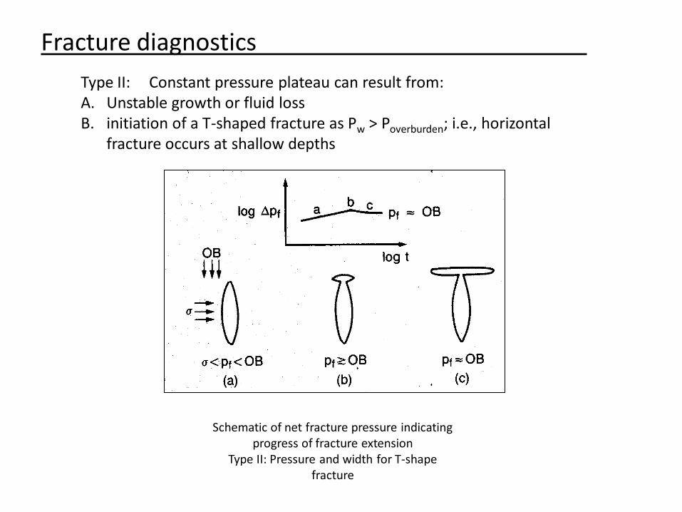
Type II: Pressure and width for T-shape fracture

Type II: Constant pressure plateau can result from:A. Unstable growth or fluid lossB. initiation of a T-shaped fracture as Pw > Poverburden; i.e., horizontal

fracture occurs at shallow depths



Type II: Pressure and width for opening natural fractures

C. Fracture pressure exceeds the natural fracture formation stress, thus opening the fissuresSubsequent fluid loss accelerates dehydration and screenoutApproximate pressure for fissures to open given by:


Type III: Fracture growth ceases…continued injection increases width of fracture and pressure, i.e, balloon effect.

Dehydration or proppant slurry bridging can result in screenout.If slope = 1 restricted fracture extension at tip. Remedy with larger pad.

If slope > 1 restriction within fracture from excessive slurry dehydration…screenout.


Fracture Geometry

Type I: KGD, constant net pressure

Type II: PKN

Type III: Penny-shaped, declines steadily and then rapidly screens out.

Type IV: Medlin & Fitch, early pressure increase, screenout when slurry reachesformation.

Downhole fracturing behavior for different fracture types

* Identify fracture behavior early to improve subsequent fracture design*


Evolution of fracture geometry

First stage- prior to reaching vertical barriers, approximate by KGD model; i.e., net pressure decreases thus negative slope

Second stage- vertical barriers force fracture length, thus Increasing pressures

Third stage- exceed minimum stress of adjacent beds resulting in height growth.

Evolution of fracture geometry and pressure during pumping


Pressure Decline Analysis• Analysis during closing and shutin periods

• Rate of pressure decline is related to fluid loss or generally to fluid loss volume, VL=Vi-Vf.

• Time required for the fracture to close defines the fluid efficiency

• With knowledge of propagation model, can estimate fracture area (Af) and width (wf).

• Can estimate:– Closure pressure, pc

– Fluid efficiency, h– Fluid loss coefficient, CL

– Fracture width, wf

– Fracture length, xf

• Two graphical solution methods– Cartesian plot of pw vs time function– Log-log plot of pressure function vs

dimensionless time function

Example of fracturing-related pressures

iV

fVh


Cartesian Method

• Plot of wellbore pressure, pw vs a time function, G(DtD) where

g functions from table or analytical solutions to limiting cases.

• Straight line during fracture closure, deviation after closure due to reservoir response.

• Fluid loss dominates

Conceptual response of pressure decline vs Nolte time function

og)Dtg(π

4)DtG( DD

pt

Δt

timepumping

eshutin timDΔt


Extension during closure

Two options

1. Early slope indicating extension

during closure, thus later slope correct

2. Early slope and time is correct

(low h case)

• Best to obtain Pc from other methods

• Correction illustrated in figure

Correcting closure time and efficiency for extension during closure


Height growth into barriers

• Initial period of reduced slope

due to reduction of height during

closure

• Opening of natural fissures would

show a constant slope because loss

to fissures would end quickly.

Closure and diagnostic growth into stress barriers.


Fracture closure with proppant

Previous analysis assumes:

1. fracture propagation not

restricted by proppant

2. Fracture closed without any

proppant effect up to Vf = V prop,

and afterwards the fracture

completely closes on the

proppant.

3. No change in compliance of the fracture with closure on proppant


Fluid Loss Coefficient, CT,

wheremp - slope of pw vs. G(DTD) plotbs - represents pressure gradient in fracture during closure

a - degree of reduction in viscosity from the wellbore to the fracture tipa = 0 constant viscosity profilea = 1 linearly varying viscosity

rp - ratio of permeable formation thickness (hn) to fracture thickness (hf)tp - pumping timeE’ - plain strain modulus = E/(1-n2)Pw - well pressure

KGDf2x

PKNfh

Eptpr

sβpmTC

KGD0.9sβ

PKNa32n

22nsβ


Efficiency without proppant, h’, with proppant,

where DtcD = Dtc/tp @ Pc on plot. Where Vprop is proppant volume fraction

Fracture length, xf, PKN KGD

Average fracture width,

Maximum fracture width,

)cDtg(

og)cDtg(η

D

D hhh )1(propV

2f

h

1*

pmsβo4g

Eiη)V(1fx

f2h

1*

pmsβo4g

Eiη)V(12f

x

fhf2x

iηVw

KGD1

PKNsβ

1

π

4wmaxw


Table 1. Time exponent (a) for different models and values of n’ and efficiency


Table 2. Closure functions for different values of a and dimensionless time


E = 4 x 106 psi hp = 50 ftn = 0.26 hf = 70 ftVi = 507.5 bbl n’ = 0.4tp = 35 min a = 0 (constant

viscosity in fracture)

Table 4. Pressure decline measurements and initial calculations

Shutin time pressure a = .5 a = 0.6

min. psi DtD G(DtD) pw,psi G(DtD) pw,psi

0.0 5990 0.00 0.000 5990 0 5990

0.9 5963 0.03 0.048 5963 0.05 5963

3.7 5882 0.11 0.183 5882 0.19 5882

6.5 5811 0.19 0.306 5811 0.32 5811

9.2 5748 0.26 0.417 5748 0.43 5748

12.0 5694 0.34 0.526 5694 0.54 5694

13.8 5659 0.39 0.593 5659 0.61 5659

15.7 5626 0.45 0.661 5626 0.68 5626

17.5 5594 0.50 0.725 5594 0.74 5594

19.4 5564 0.55 0.790 5564 0.81 5564

21.2 5534 0.61 0.850 5534 0.87 5534

23.0 5504 0.66 0.909 5504 0.93 5504

24.9 5474 0.71 0.970 5474 0.99 5474

26.7 5447 0.76 1.026 5447 1.05 5447

28.6 5418 0.82 1.085 5418 1.11 5418

30.4 5392 0.87 1.139 5392 1.16 5392

32.3 5364 0.92 1.195 5364 1.22 5364

34.1 5338 0.97 1.247 5338 1.27 5338

36.0 5314 1.03 1.302 5314 1.33 5314

37.8 5291 1.08 1.352 5291 1.38 5291

39.6 5269 1.13 1.402 5269 1.43 5269

41.5 5247 1.19 1.454 5247 1.48 5247

43.3 5228 1.24 1.502 5228 1.53 5228

46.1 5200 1.32 1.576 5200 1.61 5200

48.9 5174 1.40 1.648 5174 1.68 5174

51.6 5148 1.47 1.716 5148 1.75 5148

54.4 5126 1.55 1.786 5126 1.82 5126

57.2 5106 1.63 1.854 5106 1.89 5106

59.9 5087 1.71 1.919 5087 1.95 5087

ExampleApplication of Closure Analysis

A calibration treatment without proppant was pumped prior to the main fracturing treatment. The pertinent variables are given in Table 3, whereas the pressure decline following shutin appears in Table 4.

Table 3. Treatment and rock variables for example


1. Dimensionless time is calculated for each shutin time and is shown in Table

2. Dimensionless time function, G(DtD) is also shown in Table 4. For example, from tabulated data (Table 2), assuming a = 0.6, then go = 1.52 and DtD = 0.34 then G = 0.54

3. Inspection of the pressure

decline plot reveals the following:

Pressure decline plot for example

y = -464.25x + 5931.8

R2 = 0.999

4800

5000

5200

5400

5600

5800

6000

6200

0.0 0.5 1.0 1.5 2.0 2.5

G Function, a = .6

Pw

, p

si

Pc = 5230 psiPc, psia 5230Dtc, min 42DtcD 1.19G(DtcD) 1.49Mp 465h 0.44

35

t

pt

tDt

D

DD


PKN Model

a. Table 1 indicates for an n’ =0.4 and h = 0.44, the selection of a = 0.6 was

appropriate

b. Calculate pressure gradient term

74.003)4.0(2

2)4.0(2

32

22

an

nsb

reflecting the effect of fluid flow and viscosity during closure.

c. Calculate plain strain modulus

psixE

E 6103.421

n

d. Thickness ratio

714.070

50

f

p

ph

hr

e. Fluid leakoff coefficient

min1033.1

)103.4(35714.

)70)(74.0(464 3

6

ftx

xEtr

hmC

pp

fsp

L

b

f. Fracture half length

ftx

64570

1*

)464)(74)(.52.1(4

)103.4)(2850)(46.1(

h

1*

mβ4g

Eη)V(1x

2

6

2

fpso

if

where Vi = 507.5 bbl * 5.617 ft3/bbl = 2860 ft

3

g. Average width

inorft 174.0145.)70)(645(2

)2850(46.

h2x

ηVw

ff

i

h. Maximum width

inw

ws

30.0)74(.

)174(.44max

b

PKN Model

a. Table 1 indicates for an n’ =0.4 and h = 0.44, the selection of a = 0.6 was

appropriate


74.003)4.0(2

2)4.0(2

32

22

an

nsb

reflecting the effect of fluid flow and viscosity during closure.


psixE

E 6103.421

n

d. Thickness ratio

714.070

50

f

p

ph

hr

e. Fluid leakoff coefficient

min1033.1

)103.4(35714.

)70)(74.0(464 3

6

ftx

xEtr

hmC

pp

fsp

L

b

f. Fracture half length

ftx

64570

1*

)464)(74)(.52.1(4

)103.4)(2850)(46.1(

h

1*

mβ4g

Eη)V(1x

2

6

2

fpso

if

where Vi = 507.5 bbl * 5.617 ft3/bbl = 2860 ft

3

g. Average width

inorft 174.0145.)70)(645(2

)2850(46.

h2x

ηVw

ff

i

h. Maximum width

inw

ws

30.0)74(.

)174(.44max

b


KGD model

a. Table 1 indicates for an n’ =0.4 and h = 0.44, the correct selection of a is 0.54;

therefore using a = .6 is a reasonable approximation but may introduce some

error.


bs = 0.9


(same as PKN model)

d. Thickness ratio

(same as PKN model)

e. Fracture half length

ftx

136)70(2

1*

)464)(9)(.52.1(4

)103.4)(2850)(46.1(

2h

1*

mβ4g

Eη)V(1x

6

fpso

i2

f

f. Fluid leakoff coefficient

min1027.6

)103.4(35714.

)136(2)9.0(46423

6

ftx

xEtr

xmC

pp

fsp

L

b

g. Average width

in83.0)70)(136(2

)2850(46.

h2x

ηVw

ff

i

h. Maximum width

inw

w 05.1)83(.44

max

fracture diagnostics - new mexico tech: new mexico...

Documents