fractional heat conduction with finite wave speed in a ... · pdf filetype-i is same as the...

1132

Abstract This problem deals with the thermo-elastic interaction due to step input of temperature on the stress free boundaries of a homogene-ous visco-elastic orthotropic spherical shell in the context of a new consideration of heat conduction with fractional order generalized thermoelasticity. Using the Laplace transformation, the fundamen-tal equations have been expressed in the form of a vector-matrix differential equation which is then solved by eigen value approach and operator theory analysis. The inversion of the transformed solution is carried out by applying a method of Bellman et al (1966). Numerical estimates for thermophysical quantities are obtained for copper like material for weak, normal and strong conductivity and have been depicted graphically to estimate the effects of the fractional order parameter. Comparisons of the re-sults for different theories (TEWED (GN-III), three-phase-lag model) have also been presented and the effect of viscosity is also shown. When the material is isotropic and outer radius of the hollow sphere tends to infinity, the corresponding results agree with that of existing literature. Keywords Generalized thermo-visco-elasticity, Three-phase-lag model, Frac-tional order heat equation, Eigen value approach, Vector-matrix differential equation, Step input temperatures.

Fractional heat conduction with f inite wave speed in a thermo-visco-elast ic spherical shel l

1 INTRODUCTION

Linear viscoelasticity has been an important area of research since the period of Maxwell, Boltzman, Voigt and Kelvin. Valuable information regarding linear viscoelasticity theory may be obtained in the books of Gross (1953), Staverman and Schwrzl, Alfery and Gurnee, Ferry, Bland and Lakes. Many researchers like Biot (1954, 1955), Gurtin and Sternberg, Liioushin and Pobedria, Tanner, Huilgol and Phan-Thein have contributed notably on thermoviscoelasticity. Freudenthal has point-ed out that most of the solids, when subjected to dynamic loading, exhibit viscous effects. The Kelvin-Voigt model is one of the macroscopic mechanical models often used to describe the viscoelastic behavior of a material. The model represents the delayed elastic response subjected to

A. Sura

M. Kanoriab, *

aDepartment of Applied Mathematics, Univer-sity of Calcutta, India b Department of Applied Mathematics, Uni-versity of Calcutta, India

*Author e-mail: [email protected]

M. Kanoria et al./ Fractional heat conduction with finite wave speed in a thermo-visco-elastic spherical shell 1133

Latin American Journal of Solids and Structures 11 (2014) 1132-1162

stress when the deformation is time dependent but recoverable. The dynamic interaction of thermal and mechanical fields in solids has great practical applications in modern aeronautics, astronautics, Nuclear reactors and high-energy particle accelerators. Several researchers are working in this field. A problem involving Two-Temperature Magneto-Viscoelasticity with thermal Relaxation time in Perfect conducting medium have been solved by Ezzat and El-Karamany (2009). A two tempera-ture thermo-electro-viscoelastic problem subjected to modified Ohm's and Fourier's Laws have been solved by Ezzat et al. (2012). The classical theories of thermoelasticity involving infinite speed of propagation of thermal sig-nals, contradict physical facts. During the last five decades, non-classical theories involving finite speed of heat transportation in elastic solids have been developed to remove the paradox. In con-trast with the conventional coupled thermoelasticity theory, which involves a parabolic-type heat transport equation, these generalized theories involving a hyperbolic-type heat-transport equation are supported by experiments exhibiting the actual occurrence of wave-type heat transport in solids, called second sound effect. The first generalization to this theory is due to Lord and Shulman (1967) who formulated the generalized thermoelasticity theory involving one thermal relaxation time, which is known as extended thermo-elasticity theory (ETE). The second generalization to the coupled thermoelasticity theory due to Green and Lindsay (1972), involves two relaxation times. The third generalization to the coupled thermoelasticity theory is known as low-temperature thermoelasticity introduced by Hetnarski and Ignaczak called the H-I theory. This model is charac-terized by a system of non-linear field equations. The fourth generalization in concerned with the thermo-elasticity without energy dissipation (TE-WOED) and thermoelasticity with energy dissipation (TEWED) introduced by Green and Naghdi (1991, 1992, 1993) and provide sufficient basic modifications in the constitutive equations that per-mit treatment of a much wider class of heat flow problems, labeled as types I, II, III. The natures of these three types of constitutive equations are such that when the respective theories are linearized, type-I is same as the classical heat equation (based on Fourier’s law) whereas types II and III per-mit propagation of thermal signals at a finite speed. When Fourier conductivity is dominant the temperature equation reduces to classical Fourier’s law of heat conduction and when the effect of conductivity is negligible, the equation has undamped thermal wave solutions without energy dissi-pation. Applying the above theories of generalized thermoelasticity, several problems have been solved by Mallik and Kanoria (2008), Kar and Kanoria (2009), Islam and Kanoria (2011), Ghosh and Kanoria (2010), Banik and Kanoria (2011). Recently Roychoudhury (2007) has established a generalized mathematical model of a coupled thermoelasticity theory that includes three-phase lags in the heat flux vector, the temperature gra-dient and in the thermal displacement gradient. The more general model established reduces to the previous models as special cases. According to this model

!q = − K

!∇T (P,t +τT )+ K★

!∇ν(P,t +τν )⎡⎣ ⎤⎦ ,

where !∇ν ( "ν = T ) is the thermal displacement gradient and K★ is the additional material constant.

To study some practical relevant problems, particularly in heat transfer problems involving very short time intervals and in the problems of very high heat fluxes, the hyperbolic equation gives significantly different results than the parabolic equation. According to this phenomenon the lag-ging behavior in the heat conduction in solid should not be ignored particularly when the elapsed times during a transient process are very small, say about 710− s or the heat flux is very much high.

1134 M. Kanoria et al./Fractional heat conduction with finite wave speed in a thermo-visco-elastic spherical shell


Three-phase-lag model is very useful in the problems of nuclear boiling, exothermic catalytic reac-tions, phonon-electron interactions, phonon-scattering etc., where the delay time qτ captures the thermal wave behavior (a small scalar response in time), the phase-lag Tτ captures the effect of pho-non-electron interactions (a microscopic response in space), the other delay time ντ is effective since, in the three-phase-lag model, the thermal displacement gradient is considered as a constitu-tive variable whereas in the conventional thermoelasticity theory temperature gradient is considered as a constitutive variable. Banik and Kanoria (2012) have solved the effect of three-phase-lag in an infinite medium with a spherical cavity. The magneto-thermo-elastic responses in a perfectly con-ducting medium under three-phase-lag model have been studied by Das and Kanoria (2012). However, over the last few decades, anisotropic materials have been increasingly used. There are materials which have natural anisotropy such as zinc, magnesium, sapphire, wood, some rocks and crystals, and also there are artificially manufactured materials such as fiber-reinforced composite materials which exhibit anisotropic character. The advantage of composite materials over the tra-ditional materials lies on their valuable strength, elastic and other properties (1980). A reinforced material may be regarded to some order of approximation, as homogeneous and anisotropic elastic medium having a certain kind of elastic symmetry depending on the symmetry of reinforcement. Some glass fibre reinforced plastics may be regarded as transversely isotropic. Thus, problems of solid mechanics should not be restricted to the isotropic medium only. Increasing use of an aniso-tropic media demand that the study of elastic problems should be extended to anisotropic medium also. Differential equations of fractional order have been the focus of many studies due to their fre-quent appearance in various applications in fluid mechanics, viscoelasticity, biology, physics and engineering. The most important advantage of using fractional differential equations in these and other applications is their non-local property. It is well known that the integer order differential operator is a local operator but the fractional order differential operator is non-local. This means that the next state of a system depends not only upon its current state but also upon all of its his-torical states. This is more realistic, and this is one reason why fractional calculus has become more and more popular (1967, 1997, 1999). Fractional calculus has been used successfully to modify many existing models of physical pro-cesses. One can state that the whole theory of fractional derivatives and integrals was established in the second half of the nineteenth century. The first application of fractional derivatives was given by Abel who applied fractional calculus in the solution of an integral equation that arises in the formulation of the Tautochrone problem. The generalization of the concept of derivative and inte-gral to a non-integer order has been subjected to several approaches, and some various alternative definitions of fractional derivatives appeared in Refs. (1974, 1997, 2000). In the last few years, frac-tional calculus was applied successfully in various areas to modify many existing models of physical processes, e.g., chemistry, biology, modeling and identification, electronics, wave propagation and viscoelasticity (1971, 1974, 1983, 1984, 1997). One can refer to Padlubny (1999) for a survey of ap-plications of fractional calculus. Recently, a considerable research effort is expended to study anomalous diffusion, which is char-acterized by the time-fractional diffusion-wave equation by Kimmich (2002) as follows



ρc =κ I ξc,ii (1)

where ρ is the mass density, c is the concentration, κ is the diffusion conductivity, i the coordinate symbol, which takes the value 1, 2, 3. The notation I ξ is the Riemann-Liouville fractional integral, introduced as a natural generalization of the well-known n-fold repeated integral ( )nI f t written in a convolution-type form as in (2000). Youssef (2010) introduced another formula of heat conduction in the following form

qi +τ 0

∂qi

∂t= −KI ξ−1∇T , 0 < ξ b2,

0 < ξ # 2

(2) and a uniqueness theorem has also been proved. Ezzat established a new model of fractional heat conduction equation by using the new Taylor series expansion of time-fractional order, developed by Jumarie (2010) as

0 , 0 1,!

ii

qq K T

t

ξ ξ

ξ

τ ξξ

∂+ = − ∇ <

∂b

(3)

El-Karamany and Ezzat (2011) introduced two general models of fractional heat conduction law for a non-homogeneous anisotropic elastic solid. Uniqueness and reciprocal theorems are proved, and the convolutional variational principle is established and used to prove a uniqueness theorem with no restriction on the elasticity or thermal conductivity tensors except symmetry conditions. For fractional thermoelasticity not involving two-temperatures, El-Karamany and Ezzat (2011) estab-lished the uniqueness, reciprocal theorems and convolution variational principle. The dynamic cou-pled and Green-Naghdi thermoelasticity theories result as limit cases. The reciprocity relation in case of quiescent initial state is found to be independent of the order of differintegration. Fractional order theory of a perfect conducting thermoelastic medium not involving two temperatures was investigated by Ezzat and El-Karamany (2011). Thermal wave propagation in an infinite half-space under fractional order Green-Naghdi theory was studied by Sur and Kanoria (2012). To the authors’ knowledge, under three-phase-lag effect, no solution of visco-elastic orthotropic materials for fractional heat conduction equation has been reported. With this motivation in mind the present analysis is to study the thermoelastic stresses, displacement and temperature distribu-tion in a orthotropic hollow sphere in the context of GN-III and three-phase-lag model of general-ized thermoelasticity where the heat equation consists of some non-local fractional operator signify-ing not only the present state, but also the previous states due to sudden temperature change on the stress-free boundaries. The governing equations are formed in Laplace transform domain which is then solved by eigen-value approach and operator theory analysis. The inversion of the trans-formed solution are carried out numerically applying the method of Bellman et al. A comprehensive analysis of the result have been presented for 3P model and GN-III model for both viscous and non-viscous isotropic materials. The effect of the fractional order parameter is also discussed.



2 FORMULATION OF THE PROBLEM

We consider a homogeneous orthotropic thermo-visco-elastic spherical shell of inner radius a and outer radius b in an undisturbed state and initially at uniform temperature T0 . We introduce spherical polar coordinates (r,θ ,φ) with the center of the cavity at the origin as shown in Figure a. We consider spherically symmetric thermal problem so that the displacement component

!u = [u(r,t),0,0] and the temperature T are assumed to be functions of r and t only.

Y

x

(r=b)

Z

Figure a Visco–elastic spherical shell. The stress-strain-temperature relations in the present problem are (Kelvin-Voigt type)

τ rr = C33 1+ t0

∂∂t

⎛⎝⎜

⎞⎠⎟∂u∂r

+ C13 +C23( ) 1+ t0

∂∂t

⎛⎝⎜

⎞⎠⎟

ur− βrT ,

(4)

τθθ = C13 1+ t0

∂∂t

⎛⎝⎜

⎞⎠⎟∂u∂r

+ C11 +C12( ) 1+ t0

∂∂t

⎛⎝⎜

⎞⎠⎟

ur− βθT ,

(5)

τφφ = C23 1+ t0

∂∂t

⎛⎝⎜

⎞⎠⎟∂u∂r

+ C12 +C22( ) 1+ t0

∂∂t

⎛⎝⎜

⎞⎠⎟

ur− βφT ,

(6)

and the generalized heat conduction equation for fractional order three-phase-lag model is

1r 2

∂∂r

r 2 Kr★ Iα−1 ∂T

∂r+τν

★ Iα−1 ∂ !T∂r

+ KrτT Iα−1 ∂ !!T∂r

⎧⎨⎩

⎫⎬⎭

⎡

⎣⎢

⎤

⎦⎥ =

1+τ q

∂∂t

+τ q

2

2∂2

∂t2

⎛

⎝⎜

⎞

⎠⎟ ×

∂2

∂t2 ρCeT +T0 βr

∂u∂r

+ βθ + βφ( ) ur

⎧⎨⎩

⎫⎬⎭

⎡

⎣⎢

⎤

⎦⎥

(7)

P(r,θ,𝜙)

(r=a)

O



where τ ij (i, j = r,θ ,φ) are the stress tensor, T is the temperature increase over the reference tem-

perature T0 , Cij (i, j = 1,2,3) are the elastic constants, βi (i = r,θ ,φ) are the thermal moduli, Kr is the

coefficient of thermal conductivity along the radial direction, Kr★ is the additional material con-

stant along the radial direction, ρ is the mass density, Ce is the specific heat of the solid at con-

stant strain, 0t is the mechanical relaxation time, τT and τ q are the phase-lag of temperature gra-

dient and the phase-lag of the heat flux respectively. Also τν★ = Kr +τν Kr

★ where τν is the phase-lag of thermal displacement gradient. In the case 0rK = and 0,T q ντ τ τ= = = we arrive at the thermo-elasticity equations with energy dissipation (TEWED(GN-III)). The stress equation of motion in spherical polar co-ordinate is given by

∂τ rr

∂r+ 1

r2τ rr −τθθ −τφφ( ) = ρ ∂2u

∂t2 . (8)

Introducing the following non-dimensional quantities

U =C33

aβrT0

u, (R,S ) = ra

, ba

⎛⎝⎜

⎞⎠⎟

, σ R ,σθ ,σφ( ) = 1βrT0

τ rr ,τθθ ,τφφ( ),Θ = T

T0

, η = Gta

, G2 =C33

ρ, ′τ q , ′τν , ′τT( ) = G

aτ q ,τν ,τT( ).

Equations (4)-(8) become

σ R = 1+

t0Ga

∂∂η

⎛⎝⎜

⎞⎠⎟∂U∂R

+C13 +C23

C33

1+t0Ga

∂∂η

⎛⎝⎜

⎞⎠⎟

UR−Θ,

(9)

σθ =

C13

C33

1+t0Ga

∂∂η

⎛⎝⎜

⎞⎠⎟∂U∂R

+C11 +C12

C33

1+t0Ga

∂∂η

⎛⎝⎜

⎞⎠⎟

UR−βθ

βr

Θ,

(10)

σφ =

C23

C33

1+t0Ga

∂∂η

⎛⎝⎜

⎞⎠⎟∂U∂R

+C12 +C22

C33

1+t0Ga

∂∂η

⎛⎝⎜

⎞⎠⎟

UR−βφ

βr

Θ,

(11)

CT2Iα−1 + CK

2 + ′τνCT2( ) Iα−1 ∂

∂η+ ′τTCK

2 Iα−1 ∂2

∂η2

⎡

⎣⎢

⎤

⎦⎥

∂2Θ∂R2 + 2

R∂Θ∂R

⎛⎝⎜

⎞⎠⎟=

1+ ′τ q

∂∂η

+ 12

′τ q2 ∂2

∂η2

⎛⎝⎜

⎞⎠⎟

∂2Θ∂η2 + ε ∂2

∂η2

∂U∂R

+ M UR

⎛⎝⎜

⎞⎠⎟

⎧⎨⎪

⎩⎪

⎫⎬⎪

⎭⎪

(12)



and

1+

t0Ga

∂∂η

⎛⎝⎜

⎞⎠⎟

∂2U∂R2 + 2

R∂U∂R

− AUR2

⎧⎨⎩⎪

⎫⎬⎭⎪= ∂Θ∂R

+ ∂2U∂η2 . (13)

where

A =

C11 + 2C12 +C22 − (C13 +C23)C33

, (14)

and

M =

βθ + βφ

βr

. (15)

Also, CT

2 =Kr★

ρCeG2 , CK

2 =Kr

aρCeG and

ε =

βr2T0

ρCeC33

are dimensionless constants, ε being the thermoe-

lastic coupling constant. Where CT is the non-dimensional thermal wave velocity and CK is the damping co-efficient. The boundary conditions are given by

σ R = 0 on R = 1, S η r 0, η P 0

(16)

Θ = χ1 H (η)− H (η−η1

0 )( ) on R = 1,η> 0,

(17)

= χ2H (η) on R = S ,η>0. (18)

where χ1 and χ2 are dimensionless constants, and H (η) is the Heaviside unit step function. The above condition indicate that for time η P η1

0 there is no temperature (Θ = 0) on the inner bounda-ry and for η # 0 there is no temperature (Θ = 0) on the outer boundary. Thermal shocks are given on the boundaries of the shell (R = 1,S ). Thermal stresses in the elastic medium due to the applica-tion of these thermal shocks are calculated. We assume that the medium is at rest and undisturbed initially. The initial and the regularity conditions can be written as

U = ∂U

∂η= ∂2U∂η2 = ∂3U

∂η3 = 0 and Θ = ∂Θ

∂η= ∂2Θ∂η2 = ∂3Θ

∂η3 = 0 at η = 0, R P 0

(19)



U =Θ = ∂U

∂η= ∂Θ∂η

= 0 when R →∞. (20)

3 METHOD OF SOLUTION

Let

U (R, p),Θ(R, p){ } = U (R,η),Θ(R,η){ }

0

∞

∫ e− pηdη

with Re( p) > 0 denote the Laplace transform of U and Θ respectively.

Since we have

L Iα f (t){ } = 1

pα L f (t){ }.

On taking Laplace transform, equations (12) and (13) reduce to

d 2ΘdR2 + 2

RdΘdR

= a3 Θ + ε dUdR

+ 2UR

⎛⎝⎜

⎞⎠⎟

⎡

⎣⎢

⎤

⎦⎥ , (21)

and

d 2UdR2 + 2

RdUdR

− 2UR2 = a4

dΘdR

+ p2U⎛⎝⎜

⎞⎠⎟

, (22)

where a3 =

pα+1 1+ ′τ q p + 12

′τ q2 p2⎛

⎝⎜⎞⎠⎟

1+ ′τν p( )CT2 + p 1+ ′τT p( )CK

2 , a4 =

aa + t0 pG

and assuming M = 2.

Differentiating equation (21) with respect to R and using equation (22), we get

d 2

dR2

dΘdR

⎛⎝⎜

⎞⎠⎟+ 2

RdΘdR

⎛⎝⎜

⎞⎠⎟− 2

R2

dΘdR

⎛⎝⎜

⎞⎠⎟= a3 ε p2a4U + (1+ εa4 ) dΘ

dR⎡

⎣⎢

⎤

⎦⎥. (23)

Equations (22) and (23) can be written in the form

L U( ) = a4 p2U + a4

dΘdR

, (24)

and



L dΘ

dR⎛⎝⎜

⎞⎠⎟= εa3a4 p2U + a3 1+ εa4( ) dΘ

dR, (25)

where, we assume that A = 2, ε is the thermo-elastic coupling constant and

L ≡ d 2

dR2 +2R

ddR

− 2R2 . (26)

From equations (24) and (25), we have the vector-matrix differential equation as follows

L!V = !A !V , (27)

where

!V = U dΘdR

⎡

⎣⎢⎢

⎤

⎦⎥⎥

T

,

!A =D11 D12

D21 D22

⎡

⎣⎢⎢

⎤

⎦⎥⎥,

(28)

and D11 = a4 p2 , D12 = a4 , D21 = εa3a4 p2 ,

D22 = a3 1+ εa4( ).

4 EIGEN VALUE APPROACH

Let

!V = !X (m)ω (R,m), (29)

where m is a scalar, !X is a vector depending on R and ω (R,m) is a non-trivial solution of the scalar differential equation

Lω = m2ω . (30)

Let ω = R−1/2ω1 . Therefore, from equation (30) we have

d 2ω1

dR2 + 1R

dω1

dR− 9

4R2 + m2⎛⎝⎜

⎞⎠⎟ω1 = 0. (31)

The solution of equation (30) is

ω = A1I3/2 (mR)+ B1K3/2 (mR)⎡⎣ ⎤⎦ / R , (32)



Using equation (29) and (30) into equation (27) we get

!A !X = m2 !X , (33)

where

!X (m) is the eigen vector corresponding to the eigen value m2 . The characteristic equation corresponding to !A can be written as

m4 − (D11 + D22 )m2 + (D11D22 − D12D21) = 0. (34)

The roots of the characteristic equation (37) are of the form 2 2

1m m= and 2 22m m= , where

m12 + m2

2 = D11 + D22 , m12m2

2 = D11D22 − D12D21. (35)

Equation (34) can be written as

m4 − (a3 + a4 p2 + εa3a4 )m2 + a3a4 p2 = 0. (36)

Therefore, the positive roots of the equation (36) are

m1, m2 =

12

α ± β( ), (37)

where

α , β = a3 ± a4 p( )2

+ εa3a4. (38)

Therefore, m1 and m2 are real positive quantities.

The eigen vectors X (mj ), j = 1,2

corresponding to the eigen values mj

2 , j = 1,2 can be calculated as

!X (mj ) =X1(mj )

X2(mj )

⎡

⎣

⎢⎢

⎤

⎦

⎥⎥=

D12

− D11 − mj2( )

⎡

⎣

⎢⎢⎢

⎤

⎦

⎥⎥⎥, j = 1,2.

(39)

Therefore, from equation (29) and using equation (28) we get

U = D12 Ai I3/2 (mi R)+ Bi K3/2 (mi R)⎡⎣ ⎤⎦ / R ,

i=1,2∑ (40)



and

dΘdR

= − D11 − mi2( ) Ai I3/2 (mi R)+ Bi K3/2 (mi R)⎡⎣ ⎤⎦ / R ,

i=1,2∑ (41)

where I3/2 (mi R) and K3/2 (mi R) are the modified Bessel functions of order 3/ 2 of first and second kind respectively. Ai ’s and Bi ’s (i = 1,2) are independent of R but dependent of p and are to be determined from the boundary conditions. Using the recurrence relations of modified Bessel functions we obtain from equation (41)

Θ =

D11 − mi2( )

mi

Ai I1/2 (mi R)+ Bi K1/2 (mi R)⎡⎣ ⎤⎦ / R ,i=1,2∑ (42)

since

1R1/2 P3/2 (mR) = − d

dRP1/2 (mR)

mR1/2

⎡

⎣⎢

⎤

⎦⎥ , (43)

where P = I , K . Taking Laplace transform on the equations (9), (10) and (11) we get

24

5 3/ 2 1/ 23/ 21,2

24

5 3/ 2 1/ 23/ 21,2

( ) 2 ( )

( ) ( )

iR i i i

i i

ii i

i i

A a pa I m R m R R I m RmR

B a pa K m R RK m RmR

σ=

=

⎡ ⎤⎛ ⎞= + − +⎢ ⎥⎜ ⎟

⎢ ⎥⎝ ⎠⎣ ⎦⎡ ⎤

−⎢ ⎥⎣ ⎦

∑

∑ (44)

2 2

11 12 13 4 133/ 2 1/ 23/ 2

1, 2 33 33

2 211 12 13 4 13

3/ 2 1/ 23/ 21, 2 33 33

2( ) ( )

2( ) ( )

i ii i i

i r i

i ii i i

i r i

A C C C a p m CI m R m RI m R

C m CR

B C C C a p m CK m R m RK m R

C m CR

θθ

θ

βσβ

ββ

=

=

⎡ ⎤⎧ ⎫⎛ ⎞+ − −⎪ ⎪= + − +⎢ ⎥⎜ ⎟ ⎨ ⎬⎪ ⎪⎢ ⎥⎝ ⎠ ⎩ ⎭⎣ ⎦

⎡ ⎤⎧ ⎫⎛ ⎞+ − −⎪ ⎪− +⎢ ⎥⎜ ⎟ ⎨ ⎬⎪ ⎪⎢ ⎥⎝ ⎠ ⎩ ⎭⎣ ⎦

∑

∑ (45)

2 2

12 22 23 4 233/ 2 1/ 23/ 2

1, 2 33 33

2 212 22 23 4 23

3/ 2 1/ 23/ 21, 2 33 33

2( ) ( )

2( ) ( )

i ii i i

i r i

i ii i i

i r i


C m CR


C m CR

φφ

φ

βσ

β

ββ

=

=

⎡ ⎤⎧ ⎫⎛ ⎞+ − −⎪ ⎪= + − +⎢ ⎥⎜ ⎟ ⎨ ⎬⎪ ⎪⎢ ⎥⎝ ⎠ ⎩ ⎭⎣ ⎦

⎡ ⎤⎧ ⎫⎛ ⎞+ − −⎪ ⎪− +⎢ ⎥⎜ ⎟ ⎨ ⎬⎪ ⎪⎢ ⎥⎝ ⎠ ⎩ ⎭⎣ ⎦

∑

∑ (46)



where 13 23 335

33

3 .C C C

aC

⎛ ⎞+ += − +⎜ ⎟⎝ ⎠

Using the boundary conditions 0Rσ = on 1,R R S= = and 1

pχ′

Θ =

on 1R = , where ( )011 1 1pe ηχ χ −′ = − , 2

pχ

Θ = on .R S=

Using the recurrence relations (Watson, 1980) from equations (42) and (44) we obtain

1 11 2 12 1 13 2 14

1 21 2 22 1 23 2 24

11 31 2 32 1 33 2 34

21 41 2 42 1 43 2 44

0,0,

,

,

AW AW BW BWAW AW BW BW

AW AW BW BWp

AW AW BW BWp

χ

χ

+ + + =+ + + =

′+ + + =

+ + + =

(47)

2

41 5 3 / 2 1/ 2

24

2 5 3 / 2 1/ 2

24

1 5 3 / 2 1/ 2

24

2 5 3 / 2 1/ 2

( ) 2 ( ), , 1, 2

( ) 2 ( ), , 1, 2

( ) ( ), 3, 4; 1, 2

( ) ( ), 3, 4; 1, 2

i j j jj

i j j jj

i j jj

i j jj

a pW a I m m I m i jm

a pW a I m S m SI m S i jm

a pW a K m K m i jm

a pW a K m S SI m S i jm

⎛ ⎞= + − =⎜ ⎟⎜ ⎟⎝ ⎠

⎛ ⎞= + − =⎜ ⎟⎜ ⎟⎝ ⎠

= − = =

= − = =

(48)

and

2 24

3 1/ 2

2 24

4 1/ 21/ 2

( ),

( ),

ji j

j

ji j

j

a p mW P m

m

a p mW P m S

m S

−=

−=

where P I= for , 1, 2;i j = P K= for 3, 1i j= = and 4, 2.i j= =

From (44), the values of 1A , 2A , 1B and 2B are given as

111 12 13 141

21 22 23 242 1

31 32 33 341

41 42 43 442 2

00

.

W W W WAW W W WAW W W WB pW W W WB

p

χ

χ

−⎛ ⎞⎜ ⎟⎛ ⎞⎛ ⎞ ⎜ ⎟⎜ ⎟⎜ ⎟ ⎜ ⎟′⎜ ⎟⎜ ⎟ = ⎜ ⎟⎜ ⎟⎜ ⎟ ⎜ ⎟⎜ ⎟⎜ ⎟⎜ ⎟ ⎜ ⎟ ⎜ ⎟⎝ ⎠ ⎝ ⎠ ⎜ ⎟⎜ ⎟⎝ ⎠

(49)



5 SPECIAL CASES

For the homogeneous and transversely isotropic material 11 22 ,C C= 13 23C C= and .r θ φβ β β= =

Therefore from (9) and (10), .θ φσ σ= Hence, from (45) and (46), we can write

2 213 4

3/ 2 1/ 23/ 21,2 33

213 4

3/ 2 1/ 23/ 21,2 33

2 22 ( ) ( )

22 ( ) ( )

i iR i i

i i

ii i

i i

A C m a pI m R RI m R

C mR

B C a pK m R RK m RC mR

σ=

=

⎡ ⎤⎛ ⎞⎛ ⎞ −= − + + +⎢ ⎥⎜ ⎟⎜ ⎟

⎢ ⎥⎝ ⎠ ⎝ ⎠⎣ ⎦⎡ ⎤⎛ ⎞− + −⎢ ⎥⎜ ⎟

⎢ ⎥⎝ ⎠⎣ ⎦

∑

∑ (50)

2 2

11 12 13 4 133/ 2 1/ 23/ 2

1,2 33 33

2 211 12 13 4 13

3/ 2 1/ 23/ 21,2 33 33

2( ) ( )

2( ) ( )

i ii i i

i i

i ii i i

i i


C m CR


C m CR

θσ=

=

⎡ ⎤⎛ ⎞⎛ ⎞+ − −= + − +⎢ ⎥⎜ ⎟⎜ ⎟

⎢ ⎥⎝ ⎠ ⎝ ⎠⎣ ⎦⎡ ⎤⎛ ⎞⎛ ⎞+ − −

− +⎢ ⎥⎜ ⎟⎜ ⎟⎢ ⎥⎝ ⎠ ⎝ ⎠⎣ ⎦

∑

∑ (51)

Also for an isotropic material, 33 132 ,C Cλ µ λ= + = and ( )11 12 2C C λ µ+ = + and for a non-viscous

material, we have 0 0.t = Hence, 4 1.a = Thus, for an isotropic material, equations (45) and (46) reduce to

23/ 24

3/ 2 1/ 21, 2

23/ 24

3/ 2 1/ 21, 2

4 ( ) 2 ( ) /2

4 ( ) ( ) /2

R i i i ii i

i i ii i

a pA I m R m RI m R Rm

a pB K m R RK m R Rm

µσλ µ

µλ µ

=

=

⎡ ⎤⎛ ⎞= − + − +⎢ ⎥⎜ ⎟+⎢ ⎥⎝ ⎠⎣ ⎦

⎡ ⎤− −⎢ ⎥+⎣ ⎦

∑

∑ (52)

( )( )( )

( )( )( )

2 2 23/ 2

3/ 2 1/ 21, 2

2 2 23/ 2

3/ 2 1/ 21, 2

22 ( ) ( ) /2 2

22 ( ) ( ) /2 2

i ii i i

i i

i ii i i

i i

m p mA I m R RI m R R

m

m p mB K m R RK m R R

m

θ

λ λ µµσλ µ λ µ

λ λ µµλ µ λ µ

=

=

⎡ ⎤− + −⎢ ⎥= + +

+ +⎢ ⎥⎣ ⎦⎡ ⎤+ + −⎢ ⎥−

+ +⎢ ⎥⎣ ⎦

∑

∑ (53)

Moreover, for large value of b i.e., for large value of S , 0 ( )iK m S and 1( )iK m S tend to zero.

Thus we have

( ) ( ),R R RI Kσ σ σ= + (54)

( ) ( ).I Kθ θ θσ σ σ= + (55) Hence for large value ofb , the asymptotic expressions of ( )R Iσ and ( )Iθσ are given as



(56) 0→ as S →∞

and

(57) 0→ as S →∞

Therefore, for an infinitely extended body

2

3/ 23/ 2 1/ 2

1,2

4( ) ( ) ( ) / ,2R i i i

i i

pK B K m R RK m R Rm

µσλ µ=

⎡ ⎤= − −⎢ ⎥+⎣ ⎦∑ (58)

( )( )( )

2 2 23/ 2

3/ 2 1/ 21,2

22( ) ( ) ( ) / .2 2

i ii i i

i i

m p mK B K m R RK m R R

mθ

λ λ µµσλ µ λ µ=

⎡ ⎤+ + −⎢ ⎥= −

+ +⎢ ⎥⎣ ⎦∑ (59)

where

( ) ( )( ) ( ) ( ) ( )

01 2

1 2 3 / 2 2 1/ 2 211 2 2 2 2 2 2 2

2 1 3 / 2 1 1/ 2 2 1 2 3 / 2 2 1/ 2 1 1 2 1/ 2 1 1/ 2 2

1 4 ( ) 2 ( ),

4 ( ) ( ) ( ) ( ) 2 ( ) ( )

pe m m K m p K mB

p p m m K m K m p m m K m K m p m m K m K m

η µ λ µχµ λ µ

− ⎡ ⎤− + +⎣ ⎦= − ×⎡ ⎤− − − + + −⎣ ⎦

(60)

( ) ( )( ) ( ) ( ) ( )

01 2

2 1 3/ 2 1 1/ 2 112 2 2 2 2 2 2 2

2 1 3/ 2 1 1/ 2 2 1 2 3/ 2 2 1/ 2 1 1 2 1/ 2 1 1/ 2 2

1 4 ( ) 2 ( ).

4 ( ) ( ) ( ) ( ) 2 ( ) ( )

pe m m K m p K mB

p p m m K m K m p m m K m K m p m m K m K m

η µ λ µχµ λ µ

− ⎡ ⎤− + +⎣ ⎦= ×⎡ ⎤− − − + + −⎣ ⎦

(61)

The results agree with those of Kar and Kanoria (2007) for GN III model.

2 1

22

2 2 2 2( ) ( )

1 2 2 11 1 2 2 2 2 1 1

( )

4 1 4 1 4 1 4 11 2 1 2 1 2 1 22 2 2 2

R

m S R m S R

SIp R

p p p pe m S m R e m S m Rm S m m R m m S m m R m

χσ

µ µ µ µλ µ λ µ λ µ λ µ

− − − −

= ×

⎡ ⎤ ⎡ ⎤ ⎡ ⎤ ⎡ ⎤⎛ ⎞ ⎛ ⎞ ⎛ ⎞ ⎛ ⎞ ⎛ ⎞ ⎛ ⎞ ⎛ ⎞ ⎛ ⎞− − − × − − − − − − − × − − −⎢ ⎥ ⎢ ⎥ ⎢ ⎥ ⎢⎜ ⎟ ⎜ ⎟ ⎜ ⎟ ⎜ ⎟ ⎜ ⎟ ⎜ ⎟ ⎜ ⎟ ⎜ ⎟+ + + +⎢ ⎥ ⎢ ⎥ ⎢ ⎥ ⎢⎝ ⎠ ⎝ ⎠ ⎝ ⎠ ⎝ ⎠ ⎝ ⎠ ⎝ ⎠ ⎝ ⎠ ⎝ ⎠⎣ ⎦ ⎣ ⎦ ⎣ ⎦ ⎣ ⎦

2 2 2 22 21 2

2 11 2 2 2 1 1

4 1 4 11 2 1 22 2

p m p mp pm S m Sm m S m m m S m

µ µλ µ λ µ

⎥⎥

⎡ ⎤ ⎡ ⎤⎛ ⎞ ⎛ ⎞ ⎛ ⎞ ⎛ ⎞− −− − − − − − −⎢ ⎥ ⎢ ⎥⎜ ⎟ ⎜ ⎟ ⎜ ⎟ ⎜ ⎟+ +⎢ ⎥ ⎢ ⎥⎝ ⎠ ⎝ ⎠ ⎝ ⎠ ⎝ ⎠⎣ ⎦ ⎣ ⎦

1 2

22

2 2 2 2 2 22( ) ( )1 1 2 2

21 1 2 2 2 2 1

( )

( 2 )( ) ( 2 )( )2 1 4 1 2 1 4 11 1 2 1 12 ( 2 ) 2 2 ( 2 ) 2

m S R m S R

SIp R

m p m m p mpe R m S e Rm R m m S m m R m m S

θχσ

λ λ µ λ λ µµ µ µ µλ µ λ µ λ µ λ µ λ µ λ µ

− − − −

= ×

⎡ ⎤ ⎡ ⎤ ⎡ ⎤⎛ ⎞ ⎛ ⎞ ⎛ ⎞ ⎛ ⎞ ⎛− + − − + −− + × − − − − − + × −⎢ ⎥ ⎢ ⎥ ⎢ ⎥⎜ ⎟ ⎜ ⎟ ⎜ ⎟ ⎜ ⎟+ + + + + +⎢ ⎥ ⎢ ⎥ ⎢ ⎥⎝ ⎠ ⎝ ⎠ ⎝ ⎠ ⎝ ⎠ ⎝⎣ ⎦ ⎣ ⎦ ⎣ ⎦

2

11

2 2 2 22 21 2

2 11 2 2 2 1 1

2

4 1 4 11 2 1 22 2

pm Sm

p m p mp pm S m Sm m S m m m S m

µ µλ µ λ µ

⎡ ⎤⎞ ⎛ ⎞− −⎢ ⎥⎜ ⎟ ⎜ ⎟

⎢ ⎥⎠ ⎝ ⎠⎣ ⎦⎡ ⎤ ⎡ ⎤⎛ ⎞ ⎛ ⎞ ⎛ ⎞ ⎛ ⎞− −− − − − − − −⎢ ⎥ ⎢ ⎥⎜ ⎟ ⎜ ⎟ ⎜ ⎟ ⎜ ⎟+ +⎢ ⎥ ⎢ ⎥⎝ ⎠ ⎝ ⎠ ⎝ ⎠ ⎝ ⎠⎣ ⎦ ⎣ ⎦



6 OPERATOR THEORY ANALYSIS

Equations (12) and (13) can be expressed in the following form

( ) ( )

( )

22 1 2 2 1 2 1

12

2 2 22

12 2 2

11 ,2

T K T T K

q q

C I C C I C I D D

DU

α α αντ τ

η η

τ τ εη η η η

− − −⎡ ⎤∂ ∂′ ′+ + + Θ =⎢ ⎥∂ ∂⎣ ⎦⎛ ⎞⎧ ⎫∂ ∂ ∂ Θ ∂′ ′+ + +⎨ ⎬⎜ ⎟∂ ∂ ∂ ∂⎝ ⎠⎩ ⎭

(62)

with 2M = and

( )2

01 21 ,

t G UDD U Da η η

⎛ ⎞∂ ∂+ = Θ+⎜ ⎟∂ ∂⎝ ⎠

(63)

where 2,A = DR∂≡∂

and 12 .D

R R∂≡ +∂

Taking the Laplace transform, we have

( )1 3 3 1DD a a DUε− Θ = (64) and

( )21 4 4 .DD a p U a D− = Θ (65)

Where ( ) ( )

1 2 2

3 2 2

112

1 1

q q

T T K

p p pa

p C p p C

α

ν

τ τ

τ τ

+ ⎛ ⎞′ ′+ +⎜ ⎟⎝ ⎠=′ ′+ + +

and 40

.aaa t pG

=+

Operating 1DD on (64) and using (65) we have

( ){ }2 2 2 2 21 2 1 2 0.M m m M m m− + + Θ = (66)

Similarly, operating 1DD on (65) and using (64) we have

( ){ }2 2 2 2 21 2 1 2 0,L m m L m m U− + + = (67)

where 1L DD≡ and 1M DD≡ are the two operators and 2

1m and 22m are the roots of the quadratic

equation in 2m given by



4 2 23 3 4 4 3 4( ) 0.m a a a a p a a pε− + + + = (68)

As the solution of equation (66) and (67) we have

3 32 21,2( ) ( ) / ,i i i i

iU A I m R B K m R R

=

⎡ ⎤= +⎢ ⎥⎣ ⎦∑ (69)

and

1 12 21,2( ) ( ) / .i i i i

iC I m R D K m R R

=

⎡ ⎤Θ = +⎢ ⎥⎣ ⎦∑ (70)

Where ( )j iI m R and ( )j iK m R are the modified Bessel functions of order j of first and second

kind respectively; iA , iB , iC and iD are independent of R but dependent on .p Therefore, substituting the expressions of U and Θ in equation (65), we get

2 24

4

ii i

i

a p mC A

a m−

= (71)

and

2 24

4

.ii i

i

a p mD B

a m−

= (72)

Therefore

4 3 32 21, 2

( ) ( ) / ,i i i ii

U a A I m R B K m R R=

⎡ ⎤= +⎢ ⎥⎣ ⎦∑

(73)

2 24

1 12 21,2( ) ( ) / .i

i i i ii i

a p mC I m R D K m R R

m=

− ⎡ ⎤Θ = +⎢ ⎥⎣ ⎦∑ (74)

Equations (73) and (74) are the same as that of equations (40) and (42) (i.e., the solutions ob-

tained by Eigen-value approach). 7 NUMERICAL RESULTS AND DISCUSSIONS

To get the solutions for displacement, temperature distribution and stresses in the space-time do-main we have to apply Laplace inversion formula to the equations (40), (42), (44) and (45) respec-tively, which have been done numerically using the method of Bellman et al. (1966) for fixed value of the space variable and for iη η= , 1(1)7i = , where iη ’s are computed from roots of the shifted



Legendre polynomial of degree 7 (see Appendix) with 4.S = The computations for the state varia-bles are carried out for different values of ( 1)R R r and values of

2.04612, 3.67119. The materials chosen for nu-merical evaluation are copper material. The physical data for orthotropic material are (2009)

3 30

11 2 11 211 12

11 2 11 213 22

11 2 11 223 33

1 2

6.96 10 / , 0.0186, 20 ,

1.544 10 / , 0.617 10 / ,

0.597 10 / , 1.747 10 / ,

0.496 10 / , 1.716 10 / ,4, 3, 2, 1.2,T K

kg m T C

C N m C N mC N m C N m

C N m C N mC C

ρ ε

χ χ

= × = =

= × = ×

= × = ×

= × = ×= = = =

o

and the hypothetical values of the relaxation time parameters are taken as

7 7 7 70 1.0 10 sec, 2.0 10 sec, 1.5 10 sec, 1.0 10 secq Tt ντ τ τ− − − −= × = × = × = × .

Here, in this article we have considered three-phase-lag model. Now, for this model, the solution

of heat conduction is stable if 2,Tq

q

KK νττ τ

τ< <★ ★ where K Kν ντ τ= +★ ★ i.e., the stability condition of

Quintanilla and Racke is verified (2008). Also, for an isotropic material, the physical data are taken as (www.matweb.com).

30

12 2 12 2

01

8.96 / , 0.0186, 20 ,

1.387 10 / , 0.448 10 / ,0.23 / , 0.92 , 0.1.e

gm cm T C

dy cm dy cmC cal gm C K cal

ρ ελ µ

η

= = =

= × = ×= = =

o

o

In case of GN theory, K★ is an additional material constant depending on the material. For

copper like material, we take ( 2 ).

4eCKλ µ+

=★

The results of the numerical evaluation of the thermo-elastic stress variations and temperature distribution are illustrated in figures 1-8 for both large time ( 1.21)η = and small time ( 0.026)η = for weak conductivity ( 0.5)α = , normal conductivity ( 1.0)α = and strong conductivity ( 1.2)α = respec-tively for 3P and GN III models. In these figures, the magnitudes of the variation of stresses and temperature are observed for viscous material when the step-input temperatures are applied on the inner boundary 1R = and outer boundary 4S = of the hollow sphere. Figures 1 and 2 depict the variation of the radial stress against the radial distance R of the sphere. From the figures it is ob-served that the radial stress ( )Rσ vanishes at the inner boundary ( 1)R = and the outer boundaries ( 4)R = of the shell which satisfy our theoretical boundary conditions. The magnitude of the radial stress is maximum near 2.1R = for a strong conductive material and for GN III model. Also, for three-phase-lag model, the oscillatory nature is observed. This is due to the presence of the oscilla-

= 0.0257750, 0.138382, 0.352509, 0.693147, 1.21376,iη



tion term in the heat equation of three-phase-lag model. For weak conductivity ( 0.5)α = , the oscilla-tory nature is also seen for GN III model.

Figure 1 Rσ versus R for 0.5,1.0,1.2α = and 1.21.η =

Figure 2 represents the variation of Rσ for 0.026η = and 0.5,1.0,1.2α = respectively. It is seen that Rσ vanishes at the boundaries of the shell where there are thermal sources which agree with our theoretical boundary conditions. As may seen from the figure, the stress wave is compressive in nature near both the boundaries. Also, at earlier stage of wave propagation, both the models give close results, whereas with advancement of time time, the stress wave is propagating with different speeds. For 0.5α = , the effect of Rσ is very prominent inside the shell, whereas, for 1.0α = and

1.2α = , the radial stress vanishes for 2 3R< < and 1.5 3.5R< < respectively, which is physically plausible.

Figure 2 Rσ versus R for 0.5,1.0,1.2α = and 0.026.η =

Figures 3 and 4 are plotted to show the variation of the stress θσ along the radius of the sphere for different values of the non-local fractional parameter α and for 1.21, 0.026η = respectively. In

-‐5

-‐4

-‐3

-‐2

-‐1

0

1

2

1 1.5 2 2.5 3 3.5 4 4.5

𝜎R

R

VIS-3P(𝛼=0.5) VIS-GN-III(𝛼=0.5) VIS-3P(𝛼=1.0) VIS-GN-III(𝛼=1.0) VIS-3P(𝛼=1.2) VIS-GN-III(𝛼=1.2)

-‐3.5

-‐3

-‐2.5

-‐2

-‐1.5

-‐1

-‐0.5

0

0.5

1 1.5 2 2.5 3 3.5 4

𝜎R

R

VIS-3P(𝛼=0.5) VIS-GN-III(𝛼=0.5) VIS=3P(𝛼=1.0) VIS-GN-III(𝛼=1.0) VIS-3P(𝛼=1.2) VIS-GN-III(𝛼=1.2)



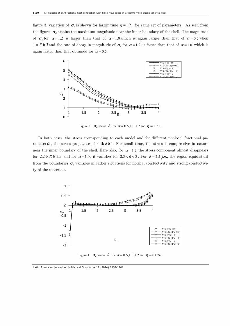
figure 3, variation of θσ is shown for larger time 1.21η = for same set of parameters. As seen from the figure, θσ attains the maximum magnitude near the inner boundary of the shell. The magnitude of θσ for 1.2α = is larger than that of 1.0α = which is again larger than that of 0.5α = when 1 3Rb b and the rate of decay in magnitude of θσ for 1.2α = is faster than that of 1.0α = which is again faster than that obtained for 0.5α = .

Figure 3 θσ versus R for 0.5,1.0,1.2α = and 1.21.η = In both cases, the stress corresponding to each model and for different nonlocal fractional pa-

rameterα , the stress propagates for 1 4.Rb b For small time, the stress is compressive in nature near the inner boundary of the shell. Here also, for 1.2,α = the stress component almost disappears for 2.2 3.5Rb b and for 1.0α = , it vanishes for 2.3 3R< < . For 2.5R = ,i.e., the region equidistant from the boundaries θσ vanishes in earlier situations for normal conductivity and strong conductivi-ty of the materials.

Figure 4 θσ versus R for 0.5,1.0,1.2α = and 0.026.η =

0

1

2

3

4

5

6

1 1.5 2 2.5 3 3.5 4

𝜎θ

R


-‐2

-‐1.5

-‐1

-‐0.5

0

0.5

1

1 1.5 2 2.5 3 3.5 4 𝜎θ

R




Figures 5 and 6 are plotted to show the variation of the stress component φσ for different frac-tional parameter .α From the figure 5, it is seen that when 1.21,η = the magnitude of φσ is maxi-mum near the inner boundary of the shell. Also it is observed that increase in the nonlocal fraction-al parameter α also increases the magnitude of the stress component .φσ For 1.0α = and 1.2,α =

the decay in magnitude of φσ is more rapid compared to that of 0.5.α = As may seen from the fig-ure, φσ is compressive near the inner boundary of the shell and the similar qualitative behavior is seen in the variation of φσ as that in figure 4.

Figure 5 φσ versus R for 0.5,1.0,1.2α = and 1.21.η =

Figure 6 φσ versus R for 0.5,1.0,1.2α = and 0.026.η =

Figures 7 and 8 depict the variation of the temperature Θ along the radius of the sphere R for different values of .α It is seen that whenever 0.1,η > (i.e., for 1.21η = ) the inner boundary of the shell is kept at zero temperature whereas for 0.026,η = the inner boundary is maintained the fixed

0

1

2

3

4

5

6

1 1.5 2 2.5 3 3.5 4

𝜎ϕ

R


-‐1.5

-‐1

-‐0.5

0

0.5

1

1 1.5 2 2.5 3 3.5 4 𝜎ϕ

R




temperature value 1 4.18χ′ = while in both situations, outer boundary maintains the same step-input-temperature 2 3.χ = For larger time, Θ attains the maximum magnitude near 2.3R = for GN III model. Whereas in the earlier situations, the magnitude of Θ decays sharply near the inner bounda-ry of the shell for 1.2α = compared to that of 0.5α = and 1.0.α = The rise in magnitude near the outer boundary is rapid also. For 1.2α = and for 0.026η = , the magnitude of the temperature al-most disappears for 1.8 3.4.R< <

Figure 7 Θ versus R for 0.5,1.0,1.2α = and 1.21.η =

Figure 8 Θ versus R for 0.5,1.0,1.2α = and 0.026.η =

Figures 9-16 are plotted to show the effect of viscosity for two set of times for weak conductive materials. Form figures 9-10 it is seen that Rσ satisfies our theoretical boundary conditions. As may seen from figure 10, it is seen that Rσ attains the maximum value for non-viscous material for both models near the inner boundary of the shell.

0

1

2

3

4

5

6

1 1.5 2 2.5 3 3.5 4

Θ

R


-‐0.5

0

0.5

1

1.5

2

2.5

3

3.5

4

4.5

1 1.5 2 2.5 3 3.5 4

Θ

R




Figure 9 Rσ versus R for 0.5α = and 1.21.η =

Figure 10 Rσ versus R for 0.5α = and 0.026.η =

Figures 11-12 are plotted to show the variation of θσ versus .R from these figures it is seen that the effect of viscosity is more prominent in GN III model compared to that of 3P lag model for a large time when 1 4.Rb b Whereas, for earlier situations, the effect of viscosity for GN III model is very prominent near the boundaries of the shell compared to the interior of the shell.

-‐2.5

-‐2

-‐1.5

-‐1

-‐0.5

0

0.5

1

1.5

1 1.5 2 2.5 3 3.5 4 𝜎R

R

V-3PHASE NV-3PHASE V-GN-III NV-GN-III

-‐4.5 -‐4

-‐3.5 -‐3

-‐2.5 -‐2

-‐1.5 -‐1

-‐0.5 0

1 1.5 2 2.5 3 3.5 4

𝜎R

R




Figure 11 θσ versus R for 0.5α = and 1.21.η =

Figure 12 θσ versus R for 0.5α = and 0.026.η =

From figures 13-14, the similar qualitative nature is seen in the variation of φσ for both viscous

and non-viscous materials.

Figure 13 φσ versus R for 0.5α = and 1.21.η =

0

0.5

1

1.5

2

2.5

3

3.5

1 1.5 2 2.5 3 3.5 4

𝜎θ

R


-‐4

-‐3

-‐2

-‐1

0

1

1 1.5 2 2.5 3 3.5 4

𝜎θ

R V-3PHASE NV-3PHASE V-GN-III NV-GN-III

0

0.5

1

1.5

2

2.5

3

3.5

1 1.5 2 2.5 3 3.5 4

𝜎ϕ

R

V-3PHASE

NV-3PHASE

V-GN-III

NV-GN-III



Figure 14 φσ versus R for 0.5α = and 0.026.η =

Figure 15 Θ versus R for 0.5α = and 1.21.η =

Figure 16 Θ versus R for 0.5α = and 0.026.η =

-‐3

-‐2.5

-‐2

-‐1.5

-‐1

-‐0.5

0

0.5

1

1 1.5 2 2.5 3 3.5 4

𝜎ϕ

R

V-3PHASE V-GN-III NV-3PHASE NV-GN-III

0

0.5

1

1.5

2

2.5

3

3.5

1 1.5 2 2.5 3 3.5 4

Θ

R

V-3PHASE

NV-3PHASE

V-GN-III

NV-GN-III

0 0.5 1

1.5 2

2.5 3

3.5 4

4.5

1 1.5 2 2.5 3 3.5 4

Θ

R




Figures 15 and 16 are plotted to show the effect of viscosity on temperature Θ for two sets of time. For both viscous and non-viscous material, the temperature satisfies our thermal boundary conditions. Also, the effect of viscosity is very prominent in earlier situations than latter. As may seen from the figures, when 1.21η = , for 3P lag model, the magnitude of Θ is larger for viscous ma-terial compared to the non-viscous material. Whereas for 0.026η = , the magnitude is larger for non-viscous material compared to the viscous material.

Figures 17-19 are plotted to show the variations of Rσ , θσ and φσ respectively against the time ηwhenever 1.4R = and 0.5.α = From these figures, it is seen that at the beginning of time, oscillatory natures are seen in the propagation of the stress components. Finally they reach to a steady state which supports the physical fact.

Figure 17 Rσ versus η for 1.4R = and 0.5.α =

Figure 18 θσ versus η for 1.4R = and 0.5.α =

-‐15

-‐10

-‐5

0

5

0 0.5 1 1.5 2 2.5 3 3.5 4

𝜎R

η

3-PHASE

GN-III

-‐15

-‐10

-‐5

0

5

0 0.5 1 1.5 2 2.5 3 3.5 4

𝜎θ

η

3-PHASE GN-III



Figure 19 φσ versus η for 1.4R = and 0.5.α =

Figures 20-22 are plotted to draw the comparison between isotropic and orthotropic material for 0.5, 1.0α = and for 0.026η = for viscous material. From figure 20, it is seen that for orthotropic ma-

terial, the stress waves are reflected from either boundary whereas for isotropic material, the propa-gation of each of the waves are found to occur. Also, amplitude of Rσ decreases with the increase of the non-local fractional parameterα .

Figure 20 Rσ versus R for 0.026η = and 0.5, 1.0.α =

Figure 21 θσ versus R for 0.026η = and 0.5, 1.0.α =

-‐60

-‐50

-‐40

-‐30

-‐20

-‐10

0

10

20

0 1 2 3 4

𝜎ϕ

η

3-PHASE GN-III

-‐4 -‐3 -‐2 -‐1 0 1 2 3 4 5

1 1.5 2 2.5 3 3.5 4

𝜎R

R

ISO(𝛼=0.5)

ISO(𝛼=1.0)

ORTHO(𝛼=0.5)

ORTHO(𝛼=1.0)

-‐2

-‐1

0

1

2

3

1 1.5 2 2.5 3 3.5 4

𝜎θ

R ISO(𝛼=0.5) ISO(𝛼=1.0) ORTHO(𝛼=0.5) ORTHO(𝛼=1.0)



Figure 21 depicts the variation of θσ versus R for isotropic and orthotropic materials. As may be seen from the figure that for an isotropic material, the oscillatory nature is observed due to the reflection as mentioned earlier. However, the magnitude of θσ is maximum near the outer boundary of the shell for an isotropic material.

Figure 22 Θ versus R for 0.026η = and 0.5, 1.0.α =

Figure 22 is plotted to show the variation of Θ versus R for two different materials. For both the materials, Θ satisfies the thermal boundary conditions. The magnitude of Θ is larger for

0.5α = than that of 1.0α = for an orthotropic material. As may seen from the figure, oscillatory behavior is seen near the boundaries for an isotropic material. It is seen that for isotropic material, when 2.5R = , i.e., at the surface equidistant from the boundaries, Θ almost disappears at the pri-mary stage of thermal load application.

8 CONCUSIONS

The problem of investigating the radial stress, hoop stress, temperature in a homogeneous isotropic viscoelastic spherical shell is studied in the light of three-phase-lag model and GN-III model in the context of space-fractional heat conduction equation. The method of Laplace Transform is used to write the basic equations in the form of a vector-matrix differential equation which is then solved by eigen-value approach. The numerical inversion of Laplace Transform is computed by the method of Bellmen. The analysis of the result permits some concluding remarks:

(i) When the time is small, ( 0.026)η = , i.e., at early stage of wave propagation, both the models give close results, whereas for comparatively large time ( 1.21)η = , significant dif-ferences are observed for weak, normal and strong conductivities ( 0.1,1.0,1.2)α = respec-tively. Also, in the earlier situations, maximum magnitude occurs for weak conductivity whereas for large time, magnitudes are maximum when conductivity is high inside the body.

-‐1

0

1

2

3

4

5

1 1.5 2 2.5 3 3.5 4

Θ

R

ISO(𝛼=0.5) ISO(𝛼=1.0) ORTHO(𝛼=0.5) ORTHO(𝛼=1.0)



(ii) It is observed that maximum magnitude of stresses will occur for viscous material and for strong conductivity ( 1.2)α = .

(iii) For an isotropic material, the maximum temperature occurs near the boundaries of the shell and it almost disappears in the interior of the shell.

(iv) The effect of Rσ is more prominent near the inner boundary for orthotropic material compared to that of an isotropic material.

Acknowledgements We are grateful to Professor S. C. Bose of the Department of Applied math-ematics, University of Calcutta, for his kind help and guidance in preparation of the paper. We also express our sincere thanks to the reviewer for his valuable suggestions for the improvement of the paper. References

Bagley, R. L.; Torvik, P. J. A theoretical basis for the application of fractional calculus to viscoelasticity. J Rhe-ol, v.27, p. 201-210, 1983. Banik, S.; Kanoria, M. Two temperature generalized thermoelastic interactions in an infinite body with a spheri-cal cavity. Int J Thermophysics, v. 32, p. 1247-1270, 2011. Banik, S.; Kanoria, M. effects of three-phase-lag on two-temperature generalized thermoelasticity for infinite me-dium with spherical cavity. Applied Mathematics and Mechanics, v. 33(4), p. 483-498, 2012. Bellman, R.; Kolaba, R. E.; Lockette, J. A. Numerical Inversion of the Laplace Transform. American Elsevier Publishing Company, New York 1966. Biot, M. A. Theory of stress-strain relations in an isotropic viscoelasticity and relaxation phenomena. J Appl Phys, v. 25(11), p. 1385-1391, 1954. Biot, M. A. Variational principal in irreversible thermodynamics with application to viscoelasticity. Phys Rev, v. 97(6), p. 1463-1469, 1955. Caputo, M. Linear models of dissipation whose Q is almost frequently independent II. Geophys J R Astron Soc , v. 13, p. 529-539, 1967. Caputo, M.; Mainardi, F. Linear model of dissipation in anelastic solids. Rivis Ta El Nuovo Cimento , v. 1, p. 161-198, 1971. Caputo, M. Vibrations of an infinite viscoelastic layer with a dissipative memory. J Acous Soc Am, v. 56, p. 897-904, 1974. Das, P.; Kanoria, M. Magneto-thermo-elastic response in a perfectly conducting medium with three-phase-lag ef-fect. Acta Mechanica, v. 223, p. 811-828, 2012. El-Karamany, A. S.; Ezzat, M. A. Convolutional variational principle, reciprocal and uniqueness theorems in linear fractional two-temperature thermoelasticity. Journal of Thermal Stresses, v. 34(3), P. 264-284, 2011. El-Karamany, A. S.; Ezzat, M. A. On the fractional Thermoelasticity. Mathematics and Mechanics of Solids , v. 16, p. 334-346, 2011. El-Karamany, A. S.; Ezzat, M. A. Fractional order theory of a prefect conducting thermoelastic medium. Can J Phys, v. 89(3), p. 311-318, 2011. Ezzat, M. A.; El-Karamany, A. S. State Space Approach of Two-Temperature Magneto-Viscoelasticity Theory with Thermal Relaxation in a Medium of Perfect Conductivity. Journal of Thermal Stresses, v. 32, p. 819-838, 2009.



Ezzat, M. A.; Zakaria, M.; El-Bary, A. A. Two-Temperature theory in thermo-electric viscoelastic material sub-jected to modified Ohm's and Fourier's Laws. Mech of Advanced Mater and Struct, v. 19, p. 453-464, 2012. Ghosh, M. K.; Kanoria, M. Study of dynamic response in a functionally graded spherically isotropic hollow sphere with temperature dependent elastic parameters. Journal of Thermal Stresses, v.33, p. 459-484, 2010. Gorenflo, R.; Mainardi, F. Fractional Calculus: Integral and Differential Equations of Fractional Orders. Frac-tals and Fractional Calculus in Continuum Mechanics. Springer, Wien, 1997. Green, A. E.; Lindsay, K. A. Thermoelasticity. J Elasticity, v. 2, p. 1-7, 1972. Green, A. E.; Naghdi, P. M. A re-examination of the basic postulate of thermo-mechanics. Proc Roy Soc Lond , v. 432, p. 171-194, 1991. Green, A. E.; Naghdi, P .M. An undamped heat wave in an elastic solid. Journal of Thermal Stresses, v. 15, p. 253-264, 1992. Green, A. E.; Naghdi, P. M. Thermoelasticity without energy dissipation. J Elasticity, v. 31, p. 189-208, 1993. Gross, B. Mathematical structure of the theories of Viscoelasticity. Hermann, Paris 1953. Hilfer, R. Application of Fraction Calculus in Physics. World Scientific, Singapore, 2000. Islam, M.; Kanoria, M. Study of dynamical response in a two dimensional transversely isotropic thick plate due to heat source. Journal of Thermal Stresses, v. 34, p. 702-723, 2011. Jumarie, G. Derivation and solutions of some fractional Black-Scholes equations in coarse-grained space and time. Application to Merton's optimal portfolio. Comput Math Appl, v. 59, p. 1142-1164, 2010. Kar, A,; Kanoria, M.: Thermoelastic interaction with energy dissipation in an unbounded body with a spherical hole. Int. J. Solids. Struct., v. 44, p. 2961-2971, 2007. Kar, A.; Kanoria, M. Generalized thermoelastic functionally graded orthotropic hollow sphere under thermal shock with three-phase-lag effect. European Journal of Mechanics A/Solids, v. 28, p. 757-767, 2009. Kimmich, R. Strange Kinetics, porous media, and NMR. J Chem Phys, v. 284,. p. 243-285, 2002. Koeller, R. C. Applications of fractional calculus to the theory of viscoelasticity. Trans ASME-J Appl Mech , v. 51, p. 299-307, 1984. Lekhnitskii, S. G. Theory of Elasticity of an anisotropic body. Mir. Moscow. Lord, H.; Shulman, Y. A. generalized theory of thermoelasticity. J Mech Phys Solid, v. 15, p. 299-309, 1967. Mainardi, F. Fractional calculus: some basic problems in continuum and statistical mechanics. In: A. Carpinteri, F. Mainardi, (eds.) Fractals and Fractional calculus in Continuum Mechanics. Springer, New York, p. 291-348, 1997. Mainardi, F.; Gorenflo, R. On Mittag-Lettler-type function in fractional evolution processes. J Comput Appl Math , v.118, p. 283-299, 2000. Mallik, S. H.; Kanoria, M. A two-dimensional problem for a transversely isotropic generalized thick plate with spatially varying heat sources. European Journal of Mechanics A/Solids, v. 27, p. 607-621, 2008. Oldham KB, Spanier J. The Fractional Calculus. Academic Press, New York, 1974. Podlubny, I. Fractional Differential Equations. Academic Press, New York 1999. Quintanilla, R.; Racke, R.: A note on stability in three-phase-lag heat conduction. Int. J. Heat Mass Transfer, v. 51, p. 24-29, 2008. Rossikhin, Yu. A.; Shitikova, M. V.; Applications of fractional calculus to dynamic problems of linear and non-linear heredity mechanics of solids. Appl Mech Rev, v. 50, p. 15-67, 1997. Roychoudhuri, S. K. On a thermoelastic three-phase-lag model. Journal of Thermal Stresses, v. 30, p. 231–238, 2007. Sur, A.; Kanoria, M. Fractional order two-temperature thermoelasticity with finite wave speed. Acta Mechanica, v. 223(12), p. 2685-2701, 2012.



www.matweb.com. Youssef, H. Theory of fractional order generalized thermoelasticity. J Heat Transfer, v. 132, p. 132:1-7, 2010.

Appendix

Let the Laplace transform of ( , )i Rσ η be given by

0

( , ) ( , ) .pj jR p e R dησ σ η η

∞−= ∫

(A.1)

We assume that ( , )j Rσ η is sufficiently smooth to permit the use of the approximate method to

apply. Substituting x e η−= in equation (A.1) we obtain

1

0

( , ) ( , ) ,pj jR p x g R x dxσ

∞−= ∫

(A.2)

where

( , ) ( , log ).j jg R x R xσ= − (A.3)

Applying the Gaussian quadrature rule to (A.2) we obtain the approximate relation

1

1

( , ) ( , ),n

pi i j i j

iW x g R x R pσ−

=

=∑ (A.4)

where ix ’s ( 1,2,3, , )i n= K are the roots of the shifted Legendre polynomial and iW ’s ( 1,2,3, , )i n= Kare the corresponding weights and 1(1) .p n=

Thus, we have

1 2

1 1 2 2

1 1 1 2 2 2

1 1 11 1 2 2

( , ) ( , ) ( , ) ( ,1)

( , ) ( , ) ( , ) ( , 2)

( , ) ( , ) ( , ) ( , )n

j j n j n j

j j n n j n j

n n nj j n j n j

W g R x W g R x W g R x RW x g R x W x g R x W x g R x R

W x g R x W x g R x W x g R x R n

σσ

σ− − −

+ + + =

+ + + =

+ + + =

LL

L L L L LL L L L L

L

Therefore



1 2

11 21

1 1 2 22

1 1 11 2

( , ) ( ,1)( , ) ( , 2)

.

( , ) ( , )

nj j

n nj j

n n nn nj n j

W W Wg R x RW x W x W xg R x R

W x W x W xg R x R n

σσ

σ

−

− − −

⎛ ⎞⎛ ⎞ ⎛ ⎞⎜ ⎟⎜ ⎟ ⎜ ⎟⎜ ⎟⎜ ⎟ ⎜ ⎟= ⎜ ⎟⎜ ⎟ ⎜ ⎟⎜ ⎟⎜ ⎟ ⎜ ⎟⎜ ⎟ ⎜ ⎟⎜ ⎟⎝ ⎠ ⎝ ⎠⎝ ⎠

LL

M M O MM ML

(A.5)

As the matrix is the product of { }idiag W multiplied by Vander monde matrix, it can be shown

that the matrix is non-singular. Hence, 1 2( , ), ( , ), , ( , )j j j ng R x g R x g R xK are known. For 7=n we have

Roots of Shifted Legendre Polynomial Corresponding Weights

2.5446043828620886E-2 6.4742483084434816E-21.2923440720030282E-1 1.3985269574463828E-12.9707742431130145E-1 1.9091502525255938E-15.0000000000000000E-1 2.0897959183673466E-17.0292257568869853E-1 1.9091502525255938E-18.7076559279969706E-1 1.3985269574463828E-19.7455395617137909E-1 6.4742483084434816E-2

From equations in (A.5) we can calculate the discrete values of ( , )j ig R x i.e., ( , );j iRσ η

( 1,2, ,7)i = K and finally using interpolation, we obtain the stress components ( , ); ( , ).i R i Rσ η θ=

fractional heat conduction with finite wave speed in a ... · pdf filetype-i is same as the...

Documents