Fractional Bosonic Strings

Victor Alfonzo Diaz1, 2, ∗ and Andrea Giusti1, 3, 4, †

1Dipartimento di Fisica e Astronomia,

Università di Bologna, Via Irnerio 46, 40126 Bologna, Italy.2I.N.F.N., Sezione di Bologna, IS - ST&FI,

via B. Pichat 6/2, 40127 Bologna, Italy3I.N.F.N., Sezione di Bologna, IS - FLAG,

via B. Pichat 6/2, 40127 Bologna, Italy.4Arnold Sommerfeld Center, Ludwig-Maximilians-Universität,

Theresienstraße 37, 80333 München, Germany.

(Dated: March 26, 2018)

AbstractThe aim of this paper is to present a simple generalization of bosonic string theory in the frame-

work of the theory of fractional variational problems. Specifically, we present a fractional extension

of the Polyakov action, for which we compute the general form of the equations of motion and

discuss the connection between the new fractional action and a generalization the Nambu-Goto

action. Consequently, we analyse the symmetries of the modified Polyakov action and try to fix

the gauge, following the classical procedures. Then we solve the equations of motion in a simplified

setting. Finally, we present an Hamiltonian description of the classical fractional bosonic string and

introduce the fractional light-cone gauge. It is important to remark that, throughout the whole

paper, we thoroughly discuss how to recover the known results as an “integer” limit of the presented

model.

Journal of Mathematical Physics 59, 033509 (2018)

DOI: 10.1063/1.5021776

∗ diaz@bo.infn.it† agiusti@bo.infn.it

1

arX

iv:1

710.

0937

0v3

[he

p-th

] 2

2 M

ar 2

018

I. INTRODUCTION

String theory is one of the very few frameworks that allows for a consistent unification of

the gravitational interaction with gauge theories. This is one of the main reasons for which

such a theory attracts a great deal of attention in the scientific community resulting to be,

in the eyes of many physicists, the leading candidate for describing gravity at the quantum

level. On this premise, it is natural to ask a simple question: Can we place all of this on a

fractional framework?

Fractional calculus has been attracting an increasing interest in both the physical and

mathematical community, reaching its peak mostly in the last decade. Indeed, this mathe-

matical approach has been applied in various areas of physics and engineering, see e.g. [1–

12]. In particular, a peculiar application of such formalism to variational problems [1, 13–15]

seems to have entered the spotlight. The aim of this section is to briefly review the notion

of fractional integral, paying particular attention to its connection with the so called class

of fractional variational problems.

From an historical viewpoint, the seed ideas of fractional calculus hides behind the Cauchy

formula concerning repeted integrations [17, 18], that reads

aJnf(t) ≡

∫ t

a

dτn

∫ τn

a

dτn−1 · · ·∫ τ2

a

dτ1 f(τ1) =1

(n− 1)!

∫ t

a

f(τ) (t− τ)n−1 dτ , (1)

where a ∈ R, t > a, n ∈ N and f(t) is assumed to be, at least, locally absolutely integrable

on t > a.

From a purely mathematical point of view, the expression of aJnf(t), defined in (2), can

be readily extended to aJαf(t) for α ∈ R+. Indeed, recalling that (n − 1)! = Γ(n), Γ(n)

is the Euler gamma function, and introducing an arbitrary positive real number α, one can

define the so called Riemann-Liouville (fractional) integral of order α > 0,

aJαf(t) ≡ 1

Γ(α)

∫ t

a

f(τ) (t− τ)α−1 dτ , (2)

for further details we invite the interested reader to refer to [2, 17, 18]. Starting from

the classical fundamental theorem of calculus one can easily define the notion of fractional

derivative as the left-inverse of the fractional integral. Clearly this condition is not enough

to guarantee the uniqueness of the definition of such an non-local operator and therefore

there exist a plethora of definitions of fractional derivatives, e.g. both the Riemann-Liouville

and the Caputo fractional derivatives are the left-inverse of (2). However, for what it might

2

concern the present work we do not need to introduce any specific generalized notion of

derivative and, therefore, we invite the the interested reader to refer to the classical textbooks

on the subject, such as [18].

The aim of this paper is to introduce the concept of a fractional time-like parameter in

the framework of classical bosonic string theory. The paper is therefore organized as follows:

First, in Section II, we briefly discuss some generalities of fractional variational problems.

In Section III, we start by fractionalizing the Polyakov action with respect to the time-like

parameter on the worldsheet.

In Section IV we compute the equations of motion and we discuss the connection between

the new Polyakov action and an extended version of the Nambu-Goto action.

In Section V and VI we discuss the symmetries of the modified Polyakov action and

we try to fix the gauge, following the classical procedures used for the ordinary conformal

gauge. After that we compute the equations of motion and we we try to solve them in this

new gauge. Always, checking the limit in which the fractional parameter α→ 1 , where we

recover the usual classical bosonic string theory result.

Then, we briefly discuss, in Section VII, the Hamiltonian description of the classical

fractional bosonic string and, after that, in Section VIII we provide some remarks on a

fractional version of the light-cone gauge and we derive the classical mass for a fractional

bosonic string.

Finally, in Section IX, we present some concluding remarks and some hints for future

research.

II. FRACTIONAL CALCULUS AND VARIATIONAL PROBLEMS

As widely discussed by Calcagni in [19, 20] in order to encode the idea of dimensional

flow in the mathematical description of physical systems, one could consider to substitute

the Lebesgue measure with the so called Lebesgue-Stieltjes measure, with a peculiar scaling,

in the action integral, i.e.

S =

∫dDxL −→ S(α) =

∫dµα(x)L , (3)

where D ∈ N is the topological dimension of the D-dimensional parameter space of the

system, dµα(x) is such that [µα] = −Dα, in momentum units, and 0 < α ≤ 1. This choice

3

is inspired by the fact that all the major quantum gravity theories predict an effective two-

dimensional behaviour of physics at very short scales. Hence, physical systems that exhibit

an effective change of their dimensionality, as a function of the scale, are likely to show some

fractional effects, at least at some level in the dynamical equations.

For sake of generality we will assume α = (α1, . . . , αD), such that 0 ≤ αi ≤ 1, with

i = 1, . . . , D.

A peculiar choice for the modified measure dµα(x), considering an absolutely continuous

framework, is given by

dµα(x) = dDx vα(x) , (4)

for some scalar function vα(x) (see [19]).

Now, let M be the d-dimensional configuration space and Ω ⊂ RD, for D ∈ N, the so

called parameter space. Denoting with TM the tangent bundle of M, we can then define a

function L, the Lagrangian, such that L ∈ C2(TM;R). Moreover, denoting with

ψ : U ⊂M → ψ(U) ⊂ Rd

a chart such that Φ ∈ C2(Ω;M) is mapped into Φ(x) ∈ ψ(U), we can explicitly write the

Lagrangian as a function of Φ(x). Now, assuming that Φ(x) satisfies some fixed Dirichlet

boundary conditions on ∂Ω, then the modified action, according to the measure (4), reads

S(α)[Φ] =

∫Ω

dDx vα(x)L(x,Φ, ∂Φ) . (5)

The corresponding equations of motion can be easily computed and they read

∂L

∂Φi(x)− ∂k

(∂L

∂(∂kΦi(x))

)=∂kvα(x)

vα(x)

∂L

∂(∂kΦi(x)), (6)

where ∂k = ∂/∂xk, with k = 1, . . . , D, Φi is the i-th component of Φ(x), with i = 1, . . . , d.

Furthermore, in (6) we have taken profit of the Einstein’s summation convention for repeated

indices.

It is now important to remark that the specific choice of the integration measure in (4)

allows us to connect the modified action principle with the general formalism of fractional

calculus. Indeed, as proposed in [16], we could introduce a specific choice of the function

vα(x), and of the parameter space Ω. In particular, if we choose

avα(ξ;x) =D∏k=1

(ξk − xk)αk−1

Γ(αk), Ωξ = (a1, ξ1) × · · · × (aD, ξD) , (7)

4

where ξ = (ξ1, . . . , ξD) and a = (a1, . . . , aD) are two constant real vectors, we have that

the corresponding Fractional Action S(α)[Φ] is defined in terms of an integral of the

convolution type that represents the D-dimensional generalization of the Riemann-Liouville

integral, i.e.

S(α)[Φ] =

∫Ωξ

dDx

D∏k=1

(ξk − xk)αk−1

Γ(αk)L(x,Φ, ∂Φ) . (8)

Thus, given the latter action functional we have that (6) turns into

∂L

∂Φi(x)− ∂k

(∂L

∂(∂kΦi(x))

)=

1− αkξk − xk

∂L

∂(∂kΦi(x)). (9)

This analysis has found several applications in theoretical physics, in particular it is im-

portant to mention the so called fractional action cosmology model [21, 22], in which a frac-

tional modification of the Einstein-Hilbert gravitational action is proposed for a Friedmann-

Robertson-Walker background.

In the next sections we analyze the implications of the discussed formalism in the classical

analysis of bosonic strings, and we will also provide some general comments on the problems

arising in the quantization procedure for the resulting Fractional Bosonic String theory.

It is also worth remarking that an Hamiltonian perspective on theories involving frac-

tional actions was hinted at in [23], and could potentially turn out to be useful for future

developments of the study presented in this paper.

III. STATEMENT OF THE PROBLEM

The propagation of strings on the d-dimensional Minkowsky spacetime R1,d−1, usually

referred to as the target space, generate a 2-dimensional surface Σ called worldsheet (WS)

defined by the map

X : Ω −→ R1,d−1 , (τ, σ) 7→X(τ, σ) = Xµ(τ, σ) , µ = 0, 1, . . . , d− 1 , (10)

called string map, where Σ = Xµ(Ω). Here, Ω = R × [0, `], with ` > 0 the length of the

string. Now, the most convenient and simple way to describe the dynamics of propagating

strings is through the use of the Polyakov action [24–28],

SP = − 1

4πα′

∫Ω

dσ dτ√−hhab(τ, σ) ∂aX(τ, σ) · ∂bX(τ, σ) , (11)

5

where a, b = τ, σ, hab(τ, σ) is called the intrinsic metric of the WS, h ≡ det(hab), a · b =

〈a, b〉η with 〈 , 〉η the Minkowsky’s bilinear form on R1,d and α′ is the Regge slope. It is now

important to remark that the dynamical variablesX(τ, σ) are d-vectors from the view point

of the target space but they are d-scalars from the WS theory. Furthermore, in general the

WS has curvature and therefore it endorse a natural connection given by the Levi-Civita

connection of hab. It also endorse a signature (−,+), which explain the minus sign in the

square root of the determinant measure in (11) and the overall minus sign.

The scope of our work is to go a little be further and introduce a generalized version of

the Polyakov action defined by

Sα,β[h,X] = − 1

4πα′

∫Ω

dσ dτ vα,β(τ, σ)√−hhab(τ, σ) ∂aX(τ, σ) · ∂bX(τ, σ) , (12)

where 0 ≤ α, β ≤ 1.

In particular, for sake of simplicity we will focus on a specific realization of such a gen-

eralization. Specifically, we will discuss extensively the case in which

Ω = Ωt = (−∞, t) × [0, `] , vα,β(x) = −∞vα,1(t; τ, σ) =(t− τ)α−1

Γ(α), (13)

where 0 < α < 1 and t ∈ R.

Therefore, in our specific example the modified action reduces to a time-fractional

Polyakov action given by

Sα ≡ −1

4πα′ Γ(α)

∫ `

0

dσ

∫ t

−∞(t− τ)α−1 dτ

[√−hhab(τ, σ) ∂aX(τ, σ) · ∂bX(τ, σ)

]. (14)

As we can see in the latter equation, basically we have modified the Polyakov action by

changing the integration over τ with a fractional integral of order 0 < α < 1 over the same

parameter.

It is easy to infer that in the limit α → 1 and t → +∞ we recover the Polyakov action

(11). It is clear that these limits do not commute, i.e. we cannot take the α-limit after the

t-limit, otherwise we encounter a divergence in the action.

IV. EQUATIONS OF MOTION

Following the discussion presented in Section II we can easily compute the equations of

motion for the general modified Polyakov action (12), and we get

δXSα,β = 0 ∂a

[vα,β(τ, σ)

√−hhab ∂bX

]= 0 , (15)

6

δhSα,β = 0 ∂aX · ∂bX −

1

2hab h

cd ∂cX · ∂dX = 0 . (16)

If we define the energy-momentum tensor of the world-sheet theory in the usual way, i.e.

Tab ≡ −4π√−h

δSα,β[h,X]

δhab=

1

α′

(∂aX · ∂bX −

1

2hab h

cd ∂cX · ∂dX), (17)

and defining the improved d’Alembert operator v as

vφ ≡1

vα,β(τ, σ)√−h

∂a

[vα,β(τ, σ)

√−hhab ∂bφ

], (18)

then Eq. (15) and (16) read,

Tab = 0 , (19)

vX = 0 . (20)

It is worth remarking that the vanishing of the stress-energy tensor allows us to con-

nect the modified Polyakov action with a generalized definition of the Nambu-Goto action.

Indeed, it is easy to see that the corresponding generalized Nambu-Goto action is given by

SαβNG[γ] = − 1

2πα′

∫Ωt

dτ dσ vα,β(τ, σ)√−γ , (21)

where γ ≡ det(γab) and γab is the induced metric on the WS, given by γab = ∂aX · ∂bX. As

suggested in [19, 20, 29], the latter equation tells us that a suitable choice of the measure

function vα,β(τ, σ), such as the fractional kernel (7), would lead to a geometrical structure

of the parameter space Ω that would resemble, in some sense, the one of a fractal.

Now, naively we have that the integration over σ in the “ordinary” bosonic string theory

carries an heavy physical significance due to its connection with the fundamental length of

the model, i.e. the string length. Our aim for this paper is to present a slightly modified

description of the evolution of the bosonic string without affecting excessively the physical

meaning associated to the fundamental parameter of the theory. Therefore, despite the fact

that our model could be carried out in a more general fashion, we will focus our attention

to the fractional action defined in (14). Hence, for the case of our concern the equations of

motion reduce to

Tab = ∂aX · ∂bX −1

2hab h

cd ∂cX · ∂dX = 0 , (22)

∂a

[(t− τ)α−1

√−hhab ∂bX

]= 0 . (23)

As we can see, these are highly non-linear partial differential equations but, due to the

symmetries of the action (14), they can be simplified, as discussed in the following section.

7

V. SYMMETRIES

First of all, we need to differentiate two different types of symmetries of the action: the

target space symmetries and the WS symmetries.

Target space symmetries

It is clear from (14) that our action is completely Poincarè invariant, that is the action

is invariant under the transformation

X(τ, σ)→ X(τ, σ) = ΛX(τ, σ) + a ,

hab(τ, σ)→ hab(τ, σ) = hab(τ, σ) ,(24)

where Λ ∈ SO(1, d− 1) and a is a constant d-vector.

Worldsheet symmetries

We have several symmetries acting on the WS:

First, we have the reparametrization invariance in the σ-direction, indeed performing the

transformation

(τ, σ) → (τ , σ) = (τ, σ − ζ(τ, σ)) ,

X(τ, σ) → X(τ , σ) = X(τ, σ)− ζ ∂σX(τ, σ)

hab(τ, σ) → hab(τ , σ) = hab(τ, σ) + ζ∂σhab + (∂aζ)hσb + (∂bζ)hσa ,

(25)

the fractional action (14) remains invariant.

Furthermore, we also have the so called Weyl Invariance, indeed the fractional action (14)

is invariant under the transformation

X(τ, σ) → X(τ , σ) = X(τ, σ) ,

hab(τ, σ) → hab(τ , σ) = e2ρ(τ,σ) hab(τ, σ).(26)

Taking profit of the WS symmetries we can reduce the degrees of freedom (d.o.f) of the

intrinsic metric hab. In 2 dimension the metric hab has 3 d.o.f, using the reparametrization

in the σ-direction we can remove one of them and, by means of the Weyl invariance, we can

8

also remove the other one. This leaves us with one d.o.f for the metric. Therefore, without

loosing of generality we can write

hab =

−1 0

0 [f 2(τ, σ)]α−1

, (27)

with f(τ, σ) an arbitrary function and in the limit α→ 1, we recover the usual flat metric.

Furthermore, we also need to respect the signature of the metric, thus hσσ(τ, σ) > 0.

Clearly, if we were to fractionalize the action with respect to both τ and σ we would lose

the σ-reparametrization invariance as well and therefore we would be left with two d.o.f.

for the intrinsic metric hab. Hence, we would have that hab = diag [f(τ, σ), g(τ, σ)], with

f(τ, σ) and g(τ, σ) two arbitrary functions of the WS parameters.

Now, using the metric (27) the equation of motion can be written as

(α− 1)f 2α−2

[f

f− 1

t− τ

]X + (α− 1)

f ′

fX ′ −X ′′ + f 2α−2 X = 0 , (28)

||fα−1 X ±X ′||2 = 0 , (29)

where the prime represents the derivative with respect to σ, the dot is understood as the

derivative with respect to τ and ||a||2 := a · a.

VI. SOLUTIONS OF THE EQUATIONS OF MOTION

The next step is try to solve these equations. Notice that Eq. (28), after the gauge fixing,

is still a set of highly non-linear equations parametrised by a real function f(τ, σ). Clearly,

it is not possible to find a solution in a closed form as a function of f(τ, σ), therefore we

can try to simplify the discussion by studying the solutions of Eq. (28) for specific choices

of this function.

Here, for sake of simplicity, we will focus only on the very simple case with f(τ, σ) = 1,

that allows us to diagonalise the intrinsic metric hab. Hence, Eq. (28) and (29) now read

X −X ′′ = α− 1

t− τX , (30)

||X ±X ′||2 = 0 , (31)

9

which clearly shows that the introduction of the time-fractional Riemann-Liouville measure

(13) leads to an extra term that resembles the contribution of fluid viscosity in classical fluid

dynamics.

Moreover, to further simplify the discussion, in the following we will consider the case

with ` = 2π together with periodic boundary conditions

X(τ, σ + 2 π) = X(τ, σ) , ∀τ ∈ (−∞, t) ,

i.e. we consider the case of a closed string.

It is important to remark that the components of X do not mix with one another in

the system given in Eq. (30), therefore the problem of finding the solutions of this system

of partial differential equations reduces to the problem of finding the solutions, compatible

with the constraints and with the cyclic boundary conditions, for the following nonlinear

partial differential equation

X −X ′′ = α− 1

t− τX , (32)

with X = X(τ, σ) a real function on the WS.

If we tackle this problem by means of the method of separation of variables, i.e. assuming

an ansatz of the form X(τ, σ) = T (τ) Σ(σ), we get that Eq. (32) rewrites as

T

T− α− 1

t− τT

T=

Σ′′

Σ. (33)

Since the right hand side depends only on σ and the left hand side only on τ , both sides are

equal to some constant value λ ∈ R. Thus,

Σ′′ = λΣ , (34)

T − α− 1

t− τT − λT = 0 (35)

We shall now compute the solutions of these two ordinary differential equations as functions

of λ. To do that we can actually distinguish three cases, namely: λ < 0, λ = 0 and λ > 0.

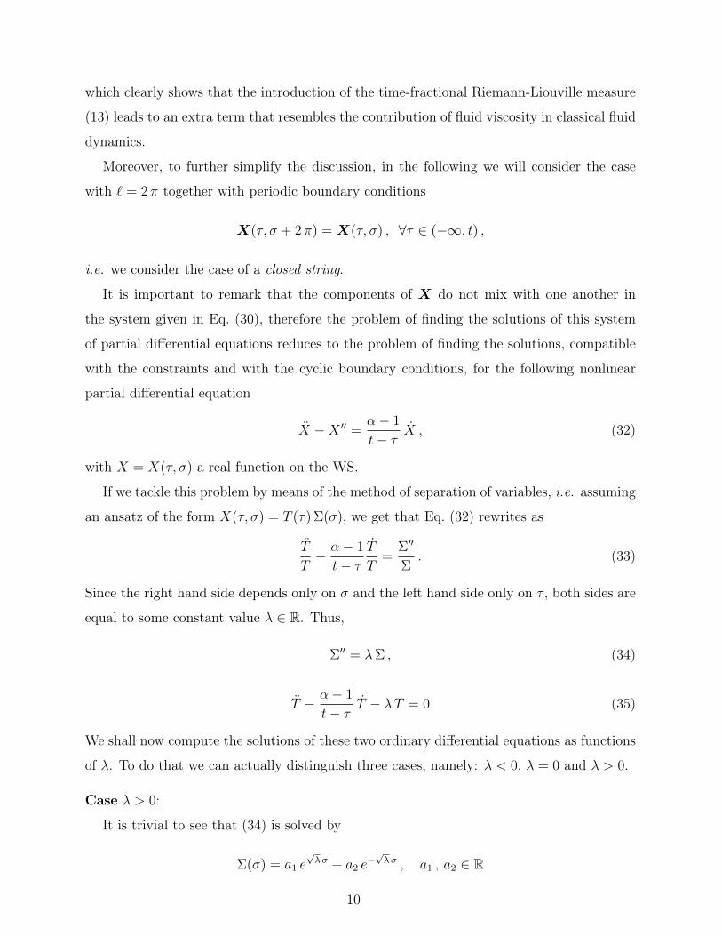
Case λ > 0:

It is trivial to see that (34) is solved by

Σ(σ) = a1 e√λσ + a2 e

−√λσ , a1 , a2 ∈ R

10

which is inconsistent with the periodic boundary conditions. Therefore, there are no solu-

tions of (32) for λ > 0.

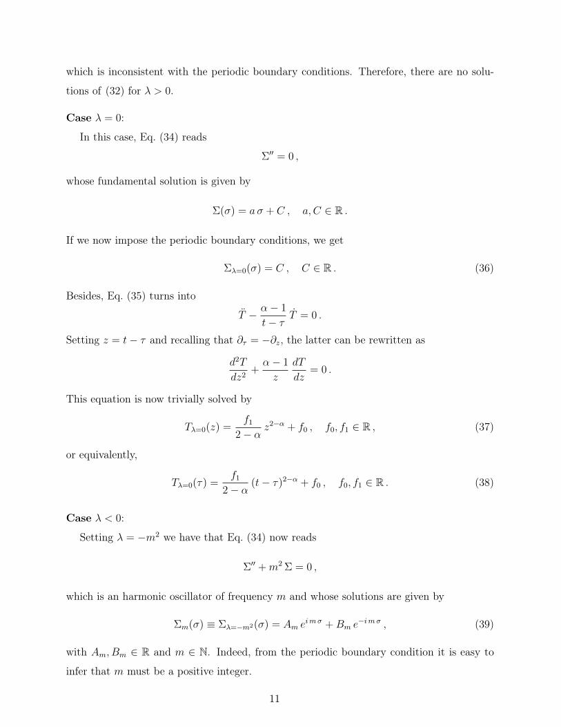
Case λ = 0:

In this case, Eq. (34) reads

Σ′′ = 0 ,

whose fundamental solution is given by

Σ(σ) = a σ + C , a, C ∈ R .

If we now impose the periodic boundary conditions, we get

Σλ=0(σ) = C , C ∈ R . (36)

Besides, Eq. (35) turns into

T − α− 1

t− τT = 0 .

Setting z = t− τ and recalling that ∂τ = −∂z, the latter can be rewritten as

d2T

dz2+α− 1

z

dT

dz= 0 .

This equation is now trivially solved by

Tλ=0(z) =f1

2− αz2−α + f0 , f0, f1 ∈ R , (37)

or equivalently,

Tλ=0(τ) =f1

2− α(t− τ)2−α + f0 , f0, f1 ∈ R . (38)

Case λ < 0:

Setting λ = −m2 we have that Eq. (34) now reads

Σ′′ +m2 Σ = 0 ,

which is an harmonic oscillator of frequency m and whose solutions are given by

Σm(σ) ≡ Σλ=−m2(σ) = Am eimσ +Bm e

−imσ , (39)

with Am, Bm ∈ R and m ∈ N. Indeed, from the periodic boundary condition it is easy to

infer that m must be a positive integer.

11

If we now consider the corresponding equation in the z = t− τ auxiliary variable, i.e.

d2T

dz2+α− 1

z

dT

dz+m2 T (z) = 0 ,

whose solutions are given by

Tm(z) ≡ Tλ=−m2(z) = zν [Cm J−ν(mz) +Dm Y−ν(mz)] , ν =2− α

2, (40)

where Cm, Dm ∈ R, m ∈ N and J is a Bessel function of the first kind and Y is a Bessel

function of the second kind.

Now, putting everything together we have that (in terms of the auxiliary variable z for

sake of clarity)

X(z, σ) = T0(z) Σ0(σ) +∞∑m=1

Tm(z) Σm(σ) , (41)

that after some algebraic manipulation turns into

X(z, σ) = C f0 + C f1z2ν

2ν+∞∑m=1

zν[am J−ν(mz) eimσ + bm Y−ν(mz) eimσ+

cm J−ν(mz) e−imσ + dm Y−ν(mz) e−imσ].

(42)

If we then recall the connection between the Bessel functions J and Y with the Hankel

functions H(1) and H(2) [30], i.e.

H(1)α (x) = Jα(x) + i Yα(x) , (43)

H(2)α (x) = Jα(x)− i Yα(x) , (44)

and that

[H(1)−ν (x)]∗ = H

(2)−ν (x) , [H

(2)−ν (x)]∗ = H

(1)−ν (x)

provided that x ∈ R and 1/2 < ν < 1, then imposing the reality condition, and with some

simple manipulations of the expansion coefficients, we get

X(z, σ) = X0 −√

2α′ z2ν

2να0 − i

√α′π

4

∞∑m=1

zν√m

[(αm e

imσ + αm e−imσ)H

(2)−ν (mz)

− (α∗m e−imσ + α∗m e

imσ)H(1)−ν (mz)

],

(45)

12

where ∗ denotes the complex conjugate.

If we then introduce a function E(ν,m ; z) such that

E(ν,m ; z) :=

√π

2zν ×

√−mH

(1)−ν (−mz) , m ∈ Z− ,

√mH

(2)−ν (mz) , m ∈ N ,

(46)

then, (45) can be expressed in a more compact form, i.e.

X(z, σ) = X0 −√

2α′ z2ν

2να0 − i

√α′

2

∑m 6=0

(αmm

eimσ +αmm

e−imσ

)E(ν,m ; z) , (47)

where αm and αm are now being redefined in a way that preserves the reality condition,

namely α∗m = α−m and α∗m = α−m for all m ∈ Z.

The last expression appears to be particularly useful due to the fact that allows us to

immediately read off the “ordinary limit” of our solution (i.e. z 7→ −τ and α → 1), indeed

recalling that [30]

H(1)α (x) =

J−α(x)− e−απi Jα(x)

i sin(απ), (48)

H(2)α (x) =

J−α(x)− eαπi Jα(x)

−i sin(απ), (49)

hence we get that

E(ν,m ; z) 7→ E (1/2,m ; τ) =

eim τ , m ∈ Z− ,

eim τ , m ∈ N ,(50)

where we have taken advantage of the known relations

H(1)−1/2(z) =

√2

π zei z , H

(2)−1/2(z) =

√2

π ze−i z .

Therefore, Eq. (47) turns into

X(z, σ) 7→ Xα=1(τ, σ) = X0−√

2α′ τ α0− i√α′

2

∑m6=0

(αmm

eimσ +αmm

e−imσ

)eim τ . (51)

which is typical normal modes expansion for bosonic strings.

Summarizing, the solution of Eq. (30) is given by

X(z, σ) = X0 −√

2α′ z2ν

2να0 − i

√α′

2

∑m6=0

(αmm

eimσ +αmm

e−imσ)E(ν,m ; z) . (52)

13

with α∗m = α−m and α∗m = α−m, ∀m ∈ Z.

Now, it is easy to see that the constraints in Eq. (31) can be easily recast into the two

following equations

||X||2 + ||X ′||2 = 0 , X ·X ′ = 0 .

Computing the derivatives of (52) one gets

X = −∂X∂z

=√

2α′ z2ν−1α0

− i z√α′

2

∑m6=0

Sgn(m)(αm e

imσ + αm e−imσ

)E(ν − 1,m ; z) ,

(53)

X ′ = −√α′

2

∑m6=0

(αm e

imσ − αm e−imσ)E(ν,m ; z) , (54)

with Sgn(m) is the sign function and where we have taken profit of

∂

∂zE(ν,m ; z) = −|m| z E(ν − 1,m ; z) . (55)

Proof. It is easy to see that [30]

∂

∂z

[zν H

(1)−ν (−mz)

]= mzν H

(1)−(ν−1)(−mz) ,

∂

∂z

[zν H

(2)−ν (mz)

]= −mzν H

(2)−(ν−1)(mz) ,

therefore, from the definition in (46) one has that

∂

∂zE(ν,m ; z) =

√π

2

∂

∂z

[zν ×

√−mH

(1)−ν (−mz) , m ∈ Z− ,

√mH

(2)−ν (mz) , m ∈ N ,

]

=

√π

2zν ×

m√−mH

(1)−(ν−1)(−mz) , m ∈ Z− ,

−m√mH

(2)−(ν−1)(mz) , m ∈ N ,

= −|m| z

[√π

2zν−1 ×

√−mH

(1)−(ν−1)(−mz) , m ∈ Z− ,

√mH

(2)−(ν−1)(mz) , m ∈ N ,

]=

= −|m| z E(ν − 1,m ; z) .

14

Then, if we now consider the expressions for X andX ′, computed above, it is easy to see

that the constraint equations do not lead, for the general 0 < α < 1, to the typical (ordinary)

Virasoro constraints. Therefore, the study of the mass spectrum for the fractional bosonic

string, at the quantum level, together with the formulation of a sort of generalized form of

the of the classical Virasoro conditions appear to be more involved and they are, thus, left

for future studies.

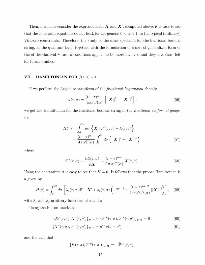
VII. HAMILTONIAN FOR f(τ, σ) = 1

If we perform the Legendre transform of the fractional Lagrangian density

L(τ, σ) =(t− τ)α−1

4πα′ Γ(α)

[||X||2 − ||X ′||2

], (56)

we get the Hamiltonian for the fractional bosonic string in the fractional conformal gauge,

i.e.

H(τ) =

∫ 2π

0

dσX ·Pτ (τ, σ)− L(τ, σ)

=

(t− τ)α−1

4πα′Γ(α)

∫ 2π

0

dσ(||X||2 + ||X ′||2

), (57)

where

Pτ (τ, σ) =∂L(τ, σ)

∂X=

(t− τ)α−1

2 π α′ Γ(α)X(τ, σ) . (58)

Using the constraints it is easy to see that H = 0. It follows that the proper Hamiltonian is

a given by

H(τ) =

∫ 2π

0

dσ

[λ1(τ, σ)Pτ ·X ′ + λ2(τ, σ)

(||Pτ ||2 +

(t− τ)2α−2

4π2α′2Γ2(α)||X ′||2

)], (59)

with λ1 and λ2 arbitrary functions of z and σ.

Using the Poison brackets

Xµ(τ, σ), Xν(τ, σ′)P.B. = Pτµ(τ, σ),Pτν(τ, σ′)P.B. = 0 ; (60)

Xµ(τ, σ),Pτν(τ, σ′)P.B. = ηµν δ(σ − σ′), (61)

and the fact that

H(τ, σ),Pτµ(τ, σ′)P.B. = −Pτµ(τ, σ) ,

15

together with

H(τ, σ), Xµ(τ, σ′)P.B. = −Xµ(τ, σ) ,

one can infer the relations

X(τ, σ) = λ1(τ, σ)X ′(τ, σ) + 2λ2(τ, σ)Pτ (τ, σ) , (62)

Pτ(τ, σ) = ∂σ [λ1(τ, σ)Pτ + 2λ2(τ, σ)X ′(τ, σ)] . (63)

Now, If one sets

λ1(τ, σ) = 0 , λ2(τ, σ) =π α′ Γ(α)

(t− τ)α−1,

we recover the canonical momentum (58) and the equation of motion (30). Therefore, this

specific choice of λ1 and λ2 defines our fractional conformal gauge.

If we now take profit of the mode expansion (52) making τ = t− z and α = 2− 2ν, the

Hamiltonian takes the form

H(z) =1

Γ(2− 2ν)

[L0(ν; z) + L0(ν; z)

], (64)

with the generalized Virasoro coefficients

L0(ν; z) ≡ 1

4

∑m∈Z

[αm ·α−m G1(ν,m; z) + 2αm · α−m G2(ν,m; z)] , (65)

L0(ν; z) ≡ 1

4

∑m∈Z

[αm · α−m G1(ν,m; z) + 2 αm ·α−m G2(ν,m; z)] . (66)

Here, we used the fact that α0 = α0, and we have also defined G1(ν, 0; z) = 2, G2(ν, 0; z) = 0,

and for m 6= 0

G1(ν,m; z) ≡ z1−2ν[z2 E(ν − 1,m ; z)E(ν − 1,−m ; z) + E(ν,m ; z)E(ν,−m ; z)

], (67)

G2(ν,m; z) ≡ z1−2ν[z2 E(ν − 1,m ; z)E(ν − 1,−m ; z)− E(ν,m ; z)E(ν,−m ; z)

]. (68)

Now, it is easy to see that in the limit ν → 1/2, we get

G1(1/2,m; z) = 2 , G2(1/2,m; z) = 0 , (69)

that leads to the well known result

H = L0 + L0 ,

=1

2

∑m∈Z

[αm ·α−m + αm · α−m] . (70)

16

VIII. FRACTIONAL LIGHT-CONE GAUGE

In the usual formalism of the bosonic strings, the Virasoro constraints arise from residual

symmetries of the system after fixing the conformal gauge (see e.g. [27, 28]). Here, we also

have some variations of the same constraints. Therefore, it is natural to think that we might

used those residual symmetries in order to set

nµXµ(τ, σ) ∝ g(τ, α) (71)

with nµ a constant vector and where g(τ, α) is such that in the limit α → 1 we have

g(τ, 1) ∝ τ . Now, selecting the light-cone gauge consist in imposing (71) with a constant

vector nµ that gives nµXµ(τ, σ) = X+(τ, σ), i.e. with nµ = 1√2(1, 0, . . . , 0, 1).

In other terms, introducing the light-cone coordinates, i.e.

X± ≡ X0 ±Xd−1

√2

,

that allows us to rewrite a vector in the Minkovsky space as X = (X+, X− , X1, . . . , Xd−2),

then a fractional version of light-cone gauge corresponds to X+(τ, σ) ∝ g(τ, α).

Therefore, denoting with

p =

∫ 2π

0

dσPτ ,

then we can define the fractional light-cone gauge as

X+(z) = −√

2α′

2να+

0 z2ν , (72)

where α+0 =

√α′

2Γ(2 − 2ν) p+ with p+ 6= 0. The main use of this gauge is usually related

to the reduction of the constraints to a simpler mathematical form. Indeed, taking profit of

the dependence on z of X+, the constrains take the form

||X||2 + ||X ′||2 = 0 2 X+ X− = X i X i +X ′iX ′i , (73)

X ·X ′ = 0 X+ X ′− = X iX ′i , (74)

where the sum over repeated indices (in this case i = 1, . . . , d − 2) is omitted, and we can

write

X− =Γ(2− 2ν) z1−2ν

2α′ p+

[X i X i +X ′iX ′i

], (75)

X ′− =Γ(2− 2ν) z1−2ν

α′ p+X iX ′i , (76)

Thus, one can see that X− is completely determined by p+ and the tranverse directions X i.

17

A. Hamiltonian and masses

We have already computed the Hamiltonian in (64), which in the fractional light-cone

coordinates can be written as

H(τ) = α′ p+ p− (t− τ)1−α

=1

Γ(2− 2ν)

[L0(ν; z) + L0(ν; z)

], (77)

with αm(αm) that ultimately reduce to αim(αim), and

p− =

∫ 2π

0

dσ Pτ−

=(t− τ)2α−2

4π α′2 p+

∫ 2π

0

dσ[X i X i +X ′iX ′i

]. (78)

Then, from the mass-shell condition we can define the mass of a fractional bosonic string,

which is given by

M2 = −||p||2 . (79)

Using the fractional light-cone gauge and the above equation, we obtain

M2(τ) =2 (t− τ)1−2ν

α′H(τ)− pi pi, (80)

that can be rewritten as

α′

2M2(τ) =

(t− τ)1−2ν

Γ(2− 2ν)

[L0(ν; τ) + L0(ν; τ)

]− α′

2pi pi. (81)

Now, if we take the limit ν → 1/2 we recover the classical result

α′

2M2 =

1

2

∑m 6=0

[αm ·α−m + αm · α−m] . (82)

IX. CONCLUSIONS

After reviewing some aspect of fractional variational problems we have presented a quite

general fractional modification of the Polyakov action and we have discussed the corre-

sponding equations of motion, together with the connection with an extended notion of

Nambu-Goto action.

Then, we have simplified the problem by considering a fractionalization of the action

with respect to the parameter τ alone. For this simplified action we have then computed

18

the corresponding equations of motion and we have studied the underlying symmetries of

the theory.

Unfortunately, due to the absence of the τ -reparametrization invariance, we are still left

with an extra degree of freedom that results in an extra functional dependence on the WS

parametrization in the induced metric hab. This makes any attempt for a general solution of

the equations of motion hopeless. In order to avoid this problem, we consider a very specific

realization of the model by setting f(τ, σ) = 1.

Then, we have computed the hamiltonian function for our model and we have also provide

a characterization for the fractional conformal gauge.

Finally, we have discussed the notion of fractional light-cone gauge and we have derived

the classical mass for a fractional bosonic string.

A precise study of the residual symmetries as well as the of the quantization of the

fractional bosonic string, even in the simplified setting, appear to be some rather involved

problems and are therefore left for future studies.

To conclude on a more physical note, on basic phenomenological principles the natural

extension of this work is the inclusion of fermionic degrees of freedom to the theory, in

order to fill the baryonic components in the Universe. The insertion of these new degrees

of freedom might be performed by adding WS supersymmetry like in the usual Ramond-

Neveu-Schwarz spinning string (RNS formalism). Furthermore, it would be interesting to

study how the superconformal gauge changes in order to accommodate these new objects.

ACKNOWLEDGMENTS

This research was partially supported by INFN, research initiatives FLAG (A.G.) and

ST&FI (V.A.D.). Moreover, the work of A.G. has been carried out in the framework of

GNFM and INdAM and the COST action Cantata.

[1] D. Baleanu, S. Muslih, Physica Scripta 72, 119 (2005).

[2] F. Mainardi, Fractional Calculus and Waves in Linear Viscoelasticity, Imperial College Press

& World Scientific, London – Singapore, 2010.

[3] I. Colombaro, A. Giusti, F. Mainardi, Z. Angew. Math. Phys. 68, 62 (2017).

19

[4] I. Colombaro, A. Giusti, F. Mainardi, Meccanica 52, 825 (2017).

[5] M. Fabrizio, Fract. Calc. Appl. Anal. 18, 1074 (2015).

[6] A. Giusti, Fract. Calc. Appl. Anal. 20, 854 (2017).

[7] A. Giusti, F. Mainardi, Eur. Phys. J. Plus 131, 206 (2016).

[8] A. Giusti, F. Mainardi, Mecanica 51, 2321 (2016).

[9] A. Giusti, J. Math. Phys. 59, 013506 (2018).

[10] P. Artale Harris, R. Garra, J. Math. Phys. 58, 063501 (2017).

[11] S. Vitali, G. Castellani, F. Mainardi, Chaos Solitons & Fractals 102, 467 (2017).

[12] S. I. Vacaru, Int. J. Theor. Phys. 51, 1338 (2012).

[13] T. M. Atanackovic, S. Konjik, S. Pilipovic, J. Phys. A: Math. Theor. 41, 095201 (2008).

[14] R. Almeida, S. Pooseh, D. F. M. Torres, Nonlinear Analysis 75, 1009 (2012).

[15] A.B. Malinowska, D.F.M. Torres, Introduction to the fractional calculus of variations, World

Scientific Publishing Company, 2012.

[16] R.A. El-Nabulsi, D.F.M. Torres, J. Math. Phys. 49, 053521 (2008).

[17] R. Gorenflo, F. Mainardi, Fractional Calculus: Integral and Differential Equations of Frac-

tional Order, in A. Carpinteri and F. Mainardi (Editors): Fractals and Fractional Calculus in

Continuum Mechanics, Springer Verlag, Wien and New York, 1997; pg. 223.

[18] A. A. Kilbas, H. M. Srivastava, J. J. Trujillo, Theory and Applications of Fractional Differential

Equations, Elsevier, Boston, 2006.

[19] G. Calcagni, Adv. Theor. Math. Phys. 16, 549 (2012).

[20] G. Calcagni, Phys. Rev. Lett. 104, 251301 (2010).

[21] V. K. Shchigolev, Mod. Phys. Lett. A 28, 1350056 (2013).

[22] V. K. Shchigolev, Eur. Phys. J. Plus 131, 256 (2016)

[23] C. Udriste, D. Opris, WSEAS Trans. Math. 7, 19 (2008).

[24] S. Deser, B. Zumino, Phys. Lett. 65B, 369 (1976).

[25] L. Brink, P. Di Vecchia, P. S. Howe, Phys. Lett. 65B, 471 (1976).

[26] A. M. Polyakov, Phys. Lett. 103B, 207 (1981).

[27] R. Blumenhagen, D. Lüst and S. Theisen, Basic Concepts of String Theory, Springer Science

& Business Media, 2012.

[28] B. Zwiebach, A first course in string theory, Cambridge university press, 2004.

[29] F.B. Tatom, Fractals 3, 217 (1995).

20

[30] M. Abramowitz and I. A. Stegun, Handbook of Mathematical Functions, with Formulas,

Graphs, and Mathematical Tables, Dover, 1972.

21