fractals - cse.unt.educse.unt.edu/~renka/4230/fractals.pdfintroduction in graphics, fractals are...

$: Fractals - cse.unt.educse.unt.edu/~renka/4230/Fractals.pdfIntroduction In graphics, fractals are used to produce natural scenes with irregular shapes, such as coastlines, clouds, forests,$
Fractals

R. J. Renka

Department of Computer Science & EngineeringUniversity of North Texas

11/14/2016

R. J. Renka Fractals

Introduction

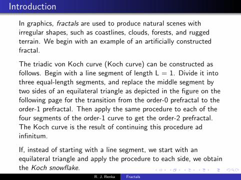
In graphics, fractals are used to produce natural scenes withirregular shapes, such as coastlines, clouds, forests, and ruggedterrain. We begin with an example of an artificially constructedfractal.

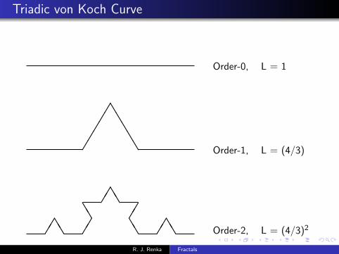
The triadic von Koch curve (Koch curve) can be constructed asfollows. Begin with a line segment of length L = 1. Divide it intothree equal-length segments, and replace the middle segment bytwo sides of an equilateral triangle as depicted in the figure on thefollowing page for the transition from the order-0 prefractal to theorder-1 prefractal. Then apply the same procedure to each of thefour segments of the order-1 curve to get the order-2 prefractal.The Koch curve is the result of continuing this procedure adinfinitum.

If, instead of starting with a line segment, we start with anequilateral triangle and apply the procedure to each side, we obtainthe Koch snowflake.


Triadic von Koch Curve

Order-0, L = 1

��TTTTT Order-1, L = (4/3)

��TT �

�TT

��TT

��TT �

�TT Order-2, L = (4/3)2


Koch Snowflake


Definition of Fractal

Since the order-k curve has length (4/3)k , the Koch curve hasinfinite length, despite being contained in a bounded region. Theextent of the curve cannot be measured in one-dimensional units(length). Magnifying an arbitrarily small piece of the curvereplicates the infinite-length curve. This is self-similarity.

Defn: A fractal is a set of points (in Rn) whose (fractal) Hausdorffdimension is greater than its topological dimension.

Roughly, topological dimension is the number of parametersneeded to specify an arbitrary point in the set: one for a smoothcurve, which is topologically equivalent (homeomorphic) to a line.More precisely, a countable set has topological dimension zero, andthe dimension of a set S is one greater than the minimumdimension of sets that can completely separate any part of S fromthe rest. Since any part of the Koch curve can be completelyseparated from the rest by a point (zero-dimensional set), theKoch curve has topological dimension 1.


Fractal Dimension

A simple planar curve has finite length

L =

∫ 1

0

√x ′(t)2 + y ′(t)2dt

for x(t), y(t) ∈ C [0, 1] and x ′(t), y ′(t) piecewise continuous; i.e.,with a finite number of discontinuities in the tangent. Thisincludes any continuous curve that we can define by a finitenumber of expressions. A fractal curve must therefore be made ofan infinite number of pieces.

A smooth (piecewise C 1) curve, sufficiently magnified, is a line:f (t + ∆t) ≈ f (t) + ∆t f ′(t). While the lengths of polygonalapproximations to a smooth curve converge to the curve length asthe number of pieces increases, the approximations diverge to ∞when applied to a nonsmooth curve. Fractals provide a means toartificially construct infinitely rugged curves and surfaces. Theirregularity is repeated at all scales rather than disappearing undermagnification.


Fractal Dimension continued

The extent of a set can only be measured in units that areconsistent with its dimension.

1 The area of a line, volume of a line or plane, and length of apoint are zero.

2 The length of a 2-D region is infinite because an infinitelylong curve can be contained in any 2-D region.

If a k-dimensional unit is used to measure an n-dimensional set, theresult will be 0 for n < k, and ∞ for n > k. The extent of a curvewith fractal dimension larger than 1 cannot be measured in units oflength. Fractal dimension D will be defined so that measuring theset with units of dimension D produces a positive finite value.


Capacity Dimension

Defn: Given S ⊂ Rk , S bounded, cover S by a set ofk-dimensional square boxes with side lengths εn = rn for0 < r < 1. Let Nn(S) be the smallest number of boxes in Rk

needed to cover S . If

D = limn→∞

log(Nn(S))

log(r−n)

exists, then S has fractal dimension D.

Note that the base of log is irrelevant because loga x/ logb x isconstant.

Example 1: Let S be a discrete set of M points in Rk . ThenNn(S) = M for large n ∈ N and any r ∈ (0, 1). Hence

D = limn→∞

log(M)

log(r−n)= 0


Capacity Dimension continued

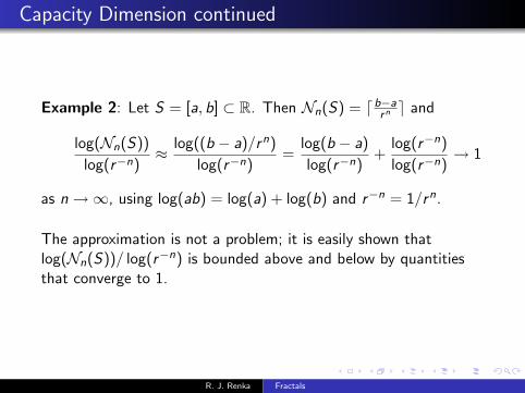
Example 2: Let S = [a, b] ⊂ R. Then Nn(S) = db−arn e and

log(Nn(S))

log(r−n)≈ log((b − a)/rn)

log(r−n)=

log(b − a)

log(r−n)+

log(r−n)

log(r−n)→ 1

as n→∞, using log(ab) = log(a) + log(b) and r−n = 1/rn.

The approximation is not a problem; it is easily shown thatlog(Nn(S))/ log(r−n) is bounded above and below by quantitiesthat converge to 1.



Example 3: Let S be the unit square [0, 1]× [0, 1], and taker = 1/2. Then

n = 1 ⇒ rn = 1/2 ⇒ N1 = 4

n = 2 ⇒ rn = 1/4 ⇒ N2 = 42

n = 3 ⇒ rn = 1/8 ⇒ N3 = 82 = 43

n = 4 ⇒ rn = 1/16 ⇒ N4 = 162 = 44

i.e., Nn = (2n)2 = 22n = 4n and

D = limn→∞

log(4n)

log(2n)= lim

n→∞

n log2(4)

n log2(2)= 2.

More generally, if the number of boxes times the box area is 1, then

Nn = 1/(rn)2 = r−2n ⇒ D = limn→∞

log(r−2n)

log(r−n)=−2n log r

−n log r= 2.

D is well-defined and independent of the choice of r .R. J. Renka Fractals


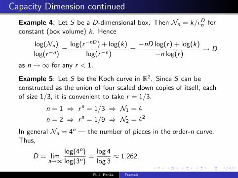
Example 4: Let S be a D-dimensional box. Then Nn = k/εDn forconstant (box volume) k . Hence

log(Nn)

log(r−n)=

log(r−nD) + log(k)

log(r−n)=−nD log(r) + log(k)

−n log(r)→ D

as n→∞ for any r < 1.

Example 5: Let S be the Koch curve in R2. Since S can beconstructed as the union of four scaled down copies of itself, eachof size 1/3, it is convenient to take r = 1/3.

n = 1 ⇒ rn = 1/3 ⇒ N1 = 4

n = 2 ⇒ rn = 1/9 ⇒ N2 = 42

In general Nn = 4n — the number of pieces in the order-n curve.Thus,

D = limn→∞

log(4n)

log(3n)=

log 4

log 3≈ 1.262.



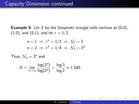
Example 6: Let S be the Sierpinski triangle with vertices at (0,0),(1,0), and (0,1), and let r = 1/2.

n = 1 ⇒ rn = 1/2 ⇒ N1 = 3

n = 2 ⇒ rn = 1/4 ⇒ N2 = 32

Thus, Nn = 3n and

D = limn→∞

log(3n)

log(2n)=

log 3

log 2≈ 1.585.



Example 7: Let S be the classical Cantor set, and let r = 1/3.

n = 1 ⇒ rn = 1/3 ⇒ N1 = 2

n = 2 ⇒ rn = 1/9 ⇒ N2 = 4

Thus, Nn = 2n and

D = limn→∞

log(2n)

log(3n)=

log 2

log 3≈ 0.631.


Random Midpoint Displacement for Curves

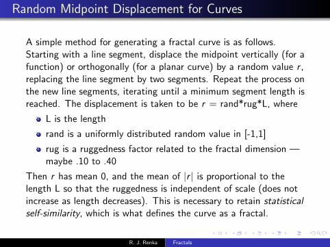
A simple method for generating a fractal curve is as follows.Starting with a line segment, displace the midpoint vertically (for afunction) or orthogonally (for a planar curve) by a random value r ,replacing the line segment by two segments. Repeat the process onthe new line segments, iterating until a minimum segment length isreached. The displacement is taken to be r = rand*rug*L, where

L is the length

rand is a uniformly distributed random value in [-1,1]

rug is a ruggedness factor related to the fractal dimension —maybe .10 to .40

Then r has mean 0, and the mean of |r | is proportional to thelength L so that the ruggedness is independent of scale (does notincrease as length decreases). This is necessary to retain statisticalself-similarity, which is what defines the curve as a fractal.


Random Midpoint Displacement for Surfaces

Consider a triangle mesh surface with the topology of a planartriangulation. One method for refining a planar triangulation is toconnect edge midpoints, replacing each triangle by four equal-areasimilar subtriangles. The random midpoint displacement methodcan be extended to a triangle mesh surface by applying it to themidpoint of each edge, and connecting the displaced midpoints ina manner that produces the same topology as the refinedtriangulation.

In the case of a polygonal surface with quadrilateral faces, the facemidpoints, along with the edge midpoints are displaced at eachiteration. The scale factor for the face midpoint should be theaverage of the four side lengths.


Mandelbrot Set

Defn: The Mandelbrot set M is the set of complex numbers c ∈ Csuch that the sequence

z0 = 0, zk = z2k−1 + c for k > 0

is bounded.

Following are some properties of M.

M is connected

The boundary of M is a fractal curve with Haussdorffdimension between 1 and 2.

M is contained in the rectangle [−2, .5]× [−1.75, 1.75].

The sequence defining M is bounded if and only if |zk | ≤ 2 forall k.


Mandelbrot Set continued

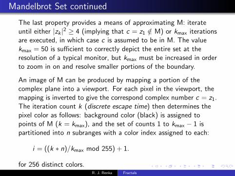
The last property provides a means of approximating M: iterateuntil either |zk |2 ≥ 4 (implying that c = z1 /∈ M) or kmax iterationsare executed, in which case c is assumed to be in M. The valuekmax = 50 is sufficient to correctly depict the entire set at theresolution of a typical monitor, but kmax must be increased in orderto zoom in on and resolve smaller portions of the boundary.

An image of M can be produced by mapping a portion of thecomplex plane into a viewport. For each pixel in the viewport, themapping is inverted to give the correspond complex number c = z1.The iteration count k (discrete escape time) then determines thepixel color as follows: background color (black) is assigned topoints of M (k = kmax), and the set of counts 1 to kmax − 1 ispartitioned into n subranges with a color index assigned to each:

i = ((k ∗ n)/kmax mod 255) + 1.

for 256 distinct colors.R. J. Renka Fractals

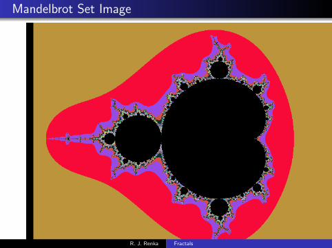
Mandelbrot Set Image


Mandelbrot Set continued

A more complete characterization of the Mandelbrot set M is asfollows. For fixed c , the set of initial values z0 for which zk

increases without bound is the basin of attraction Ac of infinity; itsboundary is the Julia set Jc ; and its complement Kc is the filledJulia set associated with c . Each such Kc is either connected orhas a one-to-one correspondence with the classical Cantor set. Mis the set of c for which Kc is connected or, equivalently, the set ofc for which Kc contains 0 (or contains c). M thus represents aninfinite number of Julia sets (magnification of M in the vicinity ofc appears similar to Kc) and is therefore not self-similar.


Iterated Function Systems

Iterated Function Systems provide a means of constructingself-similar fractals. They were popularized by Michael Barnsley in”Fractals Everywhere”, Academic Press, Inc., 1988. We begin withsome mathematics background.

Defn: A metric space (X , d) is a set X , along with a mappingd : X × X → R such that

1 0 ≤ d(p, q) <∞ and d(p, q) = 0 iff p = q ∀p, q ∈ X

2 d(p, q) = d(q, p) ∀p, q ∈ X

3 d(p, q) ≤ d(p, r) + d(r , q) ∀p, q, r ∈ X

Defn: A complete metric space is a metric space in which everyCauchy sequence converges; i.e., if d(pn, pm)→ 0 as n and mapproach ∞ independently, then d(pn, p)→ 0 for some p ∈ X .

Examples of complete metric spaces include Rn and closed subsetsof Rn with Euclidean distance.


Contraction Mapping Theorem

Let f : X → X be a transformation on a complete metric space(X , d).

Defn: A fixed point of f is a point p̄ ∈ X such that f (p̄) = p̄.

Defn: f is a contraction mapping if there exists a contractivityfactor (Lipschitz constant) s such that 0 ≤ s < 1 and

d(f (p), f (q)) ≤ sd(p, q) ∀p, q ∈ X .

Contraction Mapping Theorem: A contraction mapping f on acomplete metric space (X , d) has a unique fixed point p̄. Also, forevery point p ∈ X , f n(p)→ p̄ as n→∞.


Proof of Contraction Mapping Theorem

proof of Contraction Mapping Theorem: Let s be acontractivity factor for f , and fix p ∈ X . Then, for k = 0, 1, 2, . . .

d(p, f k(p)) ≤ d(p, f (p)) + d(f (p), f 2(p)) + · · ·+ d(f k−1(p), f k(p))

≤ (1 + s + s2 + · · ·+ sk−1)d(p, f (p))

=1− sk

1− sd(p, f (p)) ≤ 1

(1− s)d(p, f (p)).

Also, for m, n = 0, 1, 2, . . ., with m ≤ n,

d(f n(p), f m(p)) ≤ sd(f n−1(p), f m−1(p)) ≤ s2d(f n−2(p), f m−2(p))

≤ smd(f n−m(p), p) ≤ sm/(1− s)d(p, f (p)) < ε

for m, n sufficiently large. Hence, (Cauchy sequences converge)f n(p)→ p̄ as n→∞ for some p̄. Since f is contractive, f iscontinuous and f (p̄) = f (lim f n(p)) = lim f n+1(p) = p̄. Also, ifp1 = f (p1) and p2 = f (p2) then d(p1, p2) = d(f (p1), f (p2)) ≤sd(p1, p2) ⇒ (1− s)d(p1, p2) ≤ 0 ⇒ p1 = p2. �


Contraction Mappings

Example 1: Define f : R→ R by f (x) = ax + b. Then f is anaffine contraction mapping iff ∃ s < 1 such that

|f (p)− f (q)| = |ap − aq| = |a||p − q| ≤ s|p − q| ∀p, q ∈ R

iff |a| < 1. The unique fixed point is defined by p̄ = f (p̄) =ap̄ + b; i.e., p̄ = b/(1− a).

Example 2: Suppose f ∈ C 1[R] and a < b. Then ∃ α ∈ [a, b]such that

f (b)− f (a)

b − a= f ′(α).

Hence

|f (b)− f (a)| = |f ′(α)||b − a| ≤ s|b − a|

for some 0 ≤ s < 1 iff |f ′(α)| < 1. Hence, if f has rangeR(f ) ⊂ [a, b] and |f ′(α)| < 1 for all α ∈ (a, b), then f is acontraction mapping on [a, b].


Contraction Mappings continued

Example 3: Let f : R2 → R2 be defined by f (p) = Ap + b formatrix A. Then

‖f (p)− f (q)‖ = ‖Ap− Aq‖ = ‖A(p− q)‖ ≤ ‖A‖‖p− q‖,

and f is an affine contraction mapping iff ‖A‖ < 1 for operatornorm ‖ · ‖ compatible with the vector norm.

The fixed point is p̄ = Ap̄ + b⇒ p̄ = (I − A)−1b, where I − A isinvertible for ‖A‖ < 1 by the following argument. Suppose(I − A)p = 0. Then Ap = p, but ρ(A) ≤ ‖A‖ < 1 implies that 1cannot be an eigenvalue of A. Therefore p = 0.


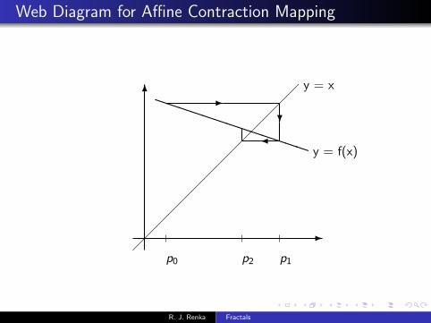
Web Diagram for Affine Contraction Mapping

-

6-

?

�

PPPPPPPPPPPPP y = f(x)

��

��

��

��

��

��

��

y = x

p0 p2 p1


Hausdorff Distance

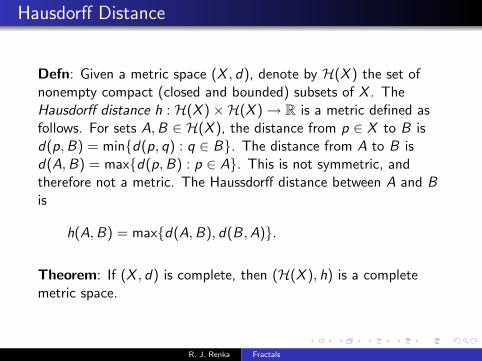
Defn: Given a metric space (X , d), denote by H(X ) the set ofnonempty compact (closed and bounded) subsets of X . TheHausdorff distance h : H(X )×H(X )→ R is a metric defined asfollows. For sets A,B ∈ H(X ), the distance from p ∈ X to B isd(p,B) = min{d(p, q) : q ∈ B}. The distance from A to B isd(A,B) = max{d(p,B) : p ∈ A}. This is not symmetric, andtherefore not a metric. The Haussdorff distance between A and Bis

h(A,B) = max{d(A,B), d(B,A)}.

Theorem: If (X , d) is complete, then (H(X ), h) is a completemetric space.


Iterated Function System

Defn: A (hyperbolic) iterated function system (IFS) is a finite setof contraction mappings on a complete metric space:w1,w2, . . . ,wN with contractivity factor s = max{s1, s2, . . . , sN}.

Theorem: Let {X ; w1,w2, . . . ,wN} be an IFS with contractivityfactor s. Define W : H(X )→ H(X ) by

W (B) = ∪Nn=1wn(B) ∀B ∈ H(X ),

where wn(B) = {wn(p) : p ∈ B}. Then W is a contractionmapping on (H(X ), h) with contractivity factor s; i.e.,

h(W (B),W (C )) ≤ sh(B,C ) ∀B,C ∈ H(X ).

Since (H(X ), h) is complete, W has a unique fixed pointA ∈ H(X ) such that

A = W (A) = ∪Nn=1wn(A) = lim

k→∞W k(B)

for any B ∈ H(X ). A is the attractor of the IFS.R. J. Renka Fractals

Outline of Proof

A contraction mapping wn is continuous, and continuous functionsmap compact sets to compact sets. Thus wn : H(X )→ H(X ) iswell-defined. It is easily shown that wn is a contraction mappingon H(X ) with contractivity factor sn. Finally, properties of h andan inductive argument show that W = ∪N

n=1 is a contractionmapping on H(X ) with contractivity factor s = max{s1, . . . , sN}.The contraction mapping theorem then applies to W . �

An IFS is similar to a dynamical system which often has anattractor, referred to as a strange attractor if it is a fractal.


IFS Examples

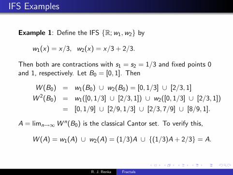
Example 1: Define the IFS {R; w1,w2} by

w1(x) = x/3, w2(x) = x/3 + 2/3.

Then both are contractions with s1 = s2 = 1/3 and fixed points 0and 1, respectively. Let B0 = [0, 1]. Then

W (B0) = w1(B0) ∪ w2(B0) = [0, 1/3] ∪ [2/3, 1]

W 2(B0) = w1([0, 1/3] ∪ [2/3, 1]) ∪ w2([0, 1/3] ∪ [2/3, 1])

= [0, 1/9] ∪ [2/9, 1/3] ∪ [2/3, 7/9] ∪ [8/9, 1].

A = limn→∞W n(B0) is the classical Cantor set. To verify this,

W (A) = w1(A) ∪ w2(A) = (1/3)A ∪ {(1/3)A + 2/3} = A.


IFS Examples continued

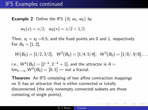
Example 2: Define the IFS {R; w1,w2} by

w1(x) = x/2, w2(x) = x/2 + 1/2.

Then, s1 = s2 =0.5, and the fixed points are 0 and 1, respectively.For B0 = [1, 2],

W (B0) = [1/2, 3/2], W 2(B0) = [1/4, 5/4], W 3(B0) = [1/8/, 9/8], . . . ;

i.e., W k(B0) = [2−k , 2−k + 1], and the attractor is A =limk→∞W k(B0) = [0, 1] — not a fractal.

Theorem: An IFS consisting of two affine contraction mappingson R has an attractor that is either connected or totallydisconnected (the only nonempty connected subsets are thoseconsisting of single points).



Example 3: Define the IFS {R2; w1,w2,w3} by

w1(p) = .5p, w2(p) = .5p + (.5, 0) w3(p) = .5p + (0, .5).

Then, s1 = s2 = s3 =0.5, and the fixed points are (0,0), (1,0), and(0,1), respectively. The attractor is a Sierpinski triangle orSierpinski gasket with vertices at the fixed points. It could bedefined as the end result of the following process. Partition atriangle into four similar equal-area subtriangles by connecting themidpoints of the edges, and then remove the middle triangle. Nowapply the same procedure to each of the three remainingsubtriangles. Continue the procedure ad infinitum. Since the areais scaled by 3/4 at each iteration, the attractor has area 0, whilethe sum of edge lengths (total perimeter of the holes) is infinite.It’s fractal dimension is log(3)/ log(2) ≈ 1.585.



Similar to the Sierpinski triangle is the Sierpinski carpet defined bythe following rule: a rectangle is partitioned into nine equal-areasubrectangles, and the middle subrectangle is removed. The rule isthen applied to each of the eight remaining subrectangles to getthe next level of approximation. This is the two-dimensionalanalogue of the classical Cantor set.

The Sierpinski sponge is the three-dimensional analogue of theCantor set. A 3-D box is uniformly partitioned into a 3 by 3 by 3grid consisting of 27 equal-volume cells (sub-boxes). The level-1approximation is then obtained by removing the center cell and thecell at the center of each of the six faces, leaving 8 corners and 12edge centers, defining 20 fixed points fi with corresponding affinecontraction mappings wi (p) = fi + (p − fi )/3. The Sierpinskisponge has infinite surface area and zero volume (fractal dimensionlog(20)/ log(3) ≈ 2.73). As a storage medium, it would require aninfinite amount of packing material to store nothing.


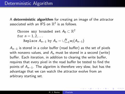
Deterministic Algorithm

A deterministic algorithm for creating an image of the attractorassociated with an IFS on R2 is as follows.

Choose any bounded set A0 ⊂ R2

for n = 1, 2, . . .Replace An−1 by An = ∪N

i=1wi (An−1)

An−1 is stored in a color buffer (read buffer) as the set of pixelswith nonzero values, and An must be stored in a second (write)buffer. Each iteration, in addition to clearing the write buffer,requires that every pixel in the read buffer be tested to find thepoints of An−1. The algoritm is therefore very slow, but has theadvantage that we can watch the attractor evolve from anarbitrary starting set.


Random Iteration Algorithm

The much faster random iteration algorithm is as follows.

Choose an initial point p = (x , y)for n = 1 to maxit

Choose wk at random (or with probability pk)Replace p with wk(p)set pixel(p)

If the initial point is a fixed point of one of the mappings, or anyother point of the attractor A, all points will be in A. Theprobabilities must satisfy pk > 0 and

∑Nk=1 pk = 1. For efficiency,

they should be chosen so that pk is approximately the ratio of thearea of wk(S) to the area of S for S ⊂ R2. Since, forwk(p) = Akp + bk , area(wk(S)) = | det(Ak)|× area(S), a goodchoice is pk = | det(Ak)|/

∑Nj=1 | det(Aj)| with an adjustment in

the case of det(Ak) = 0 so that pk > 0.


IFS Example with Probabilities

Example 4: Define the IFS {R2; w1,w2,w3,w4} by

w1(x , y) = (.25x , .5y), w2(x , y) = (.75x + .25, .5y)w3(x , y) = (.25x , .5y + .5), w4(x , y) = (.75x + .25, .5y + .5)

The contractivity factors are s1 = s3 = .5 and s2 = s4 = .75, and agood choice for the probabilities is p1 = p3 = 1/8 andp2 = p4 = 3/8. The fixed points are (0,0), (1,0), (0,1), and (1,1),and the attractor is the unit square.


The Fractal Fern

Example 5: Define the IFS {R2; w1,w2,w3,w4} by

w1(x , y) = (.85x + .04y ,−.04x + .85y + 1.6)

w2(x , y) = (.20x − .26y , .23x + .22y + 1.6)

w3(x , y) = (−.15x + .28y , .26x + .24y + .44)

w4(x , y) = (0, .16y)

with probabilities p1 = .85, p2 = p3 = .07 and p4 = .01. The fixedpoints are given by fi = (I − A)−1b for affine mappingwi (p) = Ap + b:

f1 =

[2.6556016609.958506224

], f2 =

[−0.608365019

1.871892366

]

f3 =

[0.1537693460.631552671

], f4 =

[00

]The attractor is a fractal fern contained in [−2.5, 2.5]× [0, 10].


Condensation Sets

Defn: Define w0 : H(X )→ H(X ) by w0(B) = C ∀B ∈ H(X ),where C is a fixed condensation set in H(X ).

The constant function w0 is a contraction mapping with s = 0. Itsunique fixed point is C . Even though w0 is not defined on X , itmay be included in the IFS, and the theorem still holds.

The algorithms must be modified. For the random iterationalgorithm, we include p0 > 0 and whenever w0 is to be applied top, we select a point from C at random.

For the deterministic algorithm, we simply take the initial set A0 tobe C and add to rather than replace the previous set (eliminate theclear screen command). The reason is the following. Let W (B) =∪N

n=1wn(B) and W0(B) = ∪Nn=0wn(B) = C ∪W (B) ∀B. Then

W0(C ) = C ∪W (C ) and W 20 (C ) = W0(C ∪W (C )) = C ∪

W (C ∪W (C )) = C ∪W (C ) ∪W 2(C ). Thus, the attractor is A =C ∪W (C ) ∪W 2(C ) ∪ . . .. Note that W0(A) = C ∪W (A) = A.


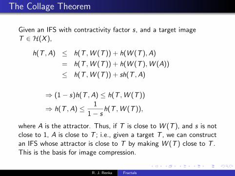
The Collage Theorem

Given an IFS with contractivity factor s, and a target imageT ∈ H(X ),

h(T ,A) ≤ h(T ,W (T )) + h(W (T ),A)

= h(T ,W (T )) + h(W (T ),W (A))

≤ h(T ,W (T )) + sh(T ,A)

⇒ (1− s)h(T ,A) ≤ h(T ,W (T ))

⇒ h(T ,A) ≤ 1

1− sh(T ,W (T )),

where A is the attractor. Thus, if T is close to W (T ), and s is notclose to 1, A is close to T ; i.e., given a target T , we can constructan IFS whose attractor is close to T by making W (T ) close to T .This is the basis for image compression.


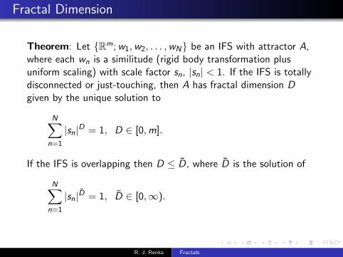
Fractal Dimension

Theorem: Let {Rm; w1,w2, . . . ,wN} be an IFS with attractor A,where each wn is a similitude (rigid body transformation plusuniform scaling) with scale factor sn, |sn| < 1. If the IFS is totallydisconnected or just-touching, then A has fractal dimension Dgiven by the unique solution to

N∑n=1

|sn|D = 1, D ∈ [0,m].

If the IFS is overlapping then D ≤ D̄, where D̄ is the solution of

N∑n=1

|sn|D̄ = 1, D̄ ∈ [0,∞).


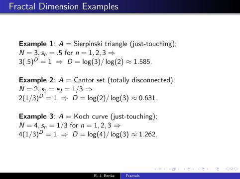
Fractal Dimension Examples

Example 1: A = Sierpinski triangle (just-touching);N = 3, sn = .5 for n = 1, 2, 3⇒3(.5)D = 1 ⇒ D = log(3)/ log(2) ≈ 1.585.

Example 2: A = Cantor set (totally disconnected);N = 2, s1 = s2 = 1/3 ⇒2(1/3)D = 1 ⇒ D = log(2)/ log(3) ≈ 0.631.

Example 3: A = Koch curve (just-touching);N = 4, sn = 1/3 for n = 1, 2, 3 ⇒4(1/3)D = 1 ⇒ D = log(4)/ log(3) ≈ 1.262.


fractals - cse.unt.educse.unt.edu/~renka/4230/fractals.pdfintroduction in graphics, fractals are...

Documents