1

Fractals, complex equations, and polynomiographs.

Summary: The generation of Mandelbrot and Julia fractals will be revisited in this article. Emphasiswill be placed on the way this fractals are created. A short overview and results of the use of themethods for creating fractals and other methods to determine the roots of complex polynomialequations will be discussed. The patterns (referred to as polynomiographs) generated with the methodof Newton-Raphson and Muller will be discussed in more detail.

1. Successive substitution: Mandelbrot and Julia fractals, finding roots.

The method with which these fractals are created has been explained in Part 1 of this series of articles.Recapitulating: a Mandelbrot fractal is generated by varying the constant C in a two-dimensional gridrepresenting the real values (X-axis) en imaginary values (Y-axis) using the equation Zn+1 = F(Zn) +C. (Z and C are complex numbers). The initial or seed value of Zn will have a fixed value and ismostly (0,0). Julia fractals have a fixed C-value , while the varying seed values of Z will be associatedwith the pixels (640 x 480) of the screen that displays the results. In both cases the coordinate valuesof the screen (screen coordinates) will be translated to the coordinate values of Z in de real/imaginarycoordinate system.

For my investigation I have used the following formula F(Z) = Z9- C.Z6 + C.Z3- Z + C=0 (1)to generate Mandelbrot and Julia fractals.To be able to use the method of successive substitution in order to create these fractals formula (1)is restated as: Zn+1 = Zn

9- C.(Zn6 - Zn

3- 1) (2)The seed value of Z chosen for this exercise is 0.5 + 0.5i in three cases in which the values for C arerespectively:rmin, rmax, imax, imin (min real value, max real value, max imaginary value, min imaginary value)or in other words the top left real world value of the screen is rmin + imax.i and the bottom right realworld value is rmax + imin.i.

The fractals are named mandel1 for C = -1, 1, 1, -1mandel2 for C = -.4, -.2, -.6, -.8, andmandel3 for C = -.38, -.36, -.62, -.64

The black areas represent the complex values of Z for which the method of successive substitutiondoes not diverge. These areas are referred to as the Mandelbrot set. The white rectangles in mandel1identifies the fractal in mandel2 and the white rectangle in mandel2 to mandel3.

2

3

For generating Julia fractals use is made of three methods: successive substitution, modifiedsuccessive substitution and a modified Wegstein method.The formula�s for these method are:

Zn+1 = F(Zn) + Zn (3) Zn+1 = D.Zn + (1-D).F(Zn) (4)

".Zn+1 = F(Zn) + ("-1).Zn (5)Zn+1 = D.Zn + (1-D).{F(Zn) + ("-1).Zn}/" (6)

See also part 2 for further explanations about these methods. Formula (4) is known as Wegstein�smethod in which D is known as the relaxation factor. Formula�s (4), (5), and (6) are not reallyintended to generate fractals. Formula (5) is a modified version of the method of successivesubstitution and can be used to make sure that the use of the method of successive substitution doesconverge to a root and does not diverge. Formula (5) can be used to assist or accelerating theiteration process in finding the roots of the original equation (1). However the resulting picturesdisplay the characteristics of fractals. Due to the fact that these are not fractals in the real sense I referto them as compromised fractals.I shall refer to the formula (6) as the modified Wegstein method. In the unmodified version of theWegstein method the value of " = 1. I furthermore refer to the constant " as the modification factor.

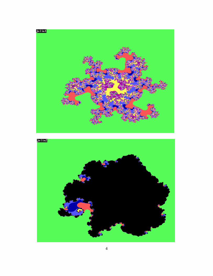
I have generated Julia fractals with methods (3) and (6) and counted the times that a root (or morethan one root) was found. Formula (3) generates normal Julia fractals. The application of formula (6)results in more roots (the seed values represented in the black areas converge to those roots), whilethe total picture represents a compromised fractal. The constant C is in all these four cases -.37 -.63*i. For julia1 the world coordinates of the seed values for Z are associated with the screencoordinates. Here Z contains the 640x480 complex numbers which are all located between -1.6, 1.2,1.6, -1.2 (xleft,xrgt,ytop,ybtm) or (rmin, rmax, imax, imin). Here 3 times a root (probably the same)was found. Julia 2 is like julia1 but the modification factor " = 2. This is a compromised fractal; julia3is like julia1 with " = 3 and a relaxation factor D = 0.1.For julia 2 more than 120.000 times and for julia3 approx. 140.000 times roots were found.

Conjecture 1: There exist a combination of a value of " and a value of D for which certain rootsof any higher degree complex polynomial can be found with the modified Wegstein method.

For julia 4 the window of the world coordinates is defined by the values -1.04, -.48, -0.08, -.64(xleft,xrgt,ytop,ybtm) or (rmin, rmax, imax, imin). Here 82647 times roots were found. Julia4 alsohas a modification factor of 3 and a relaxation factor of 0.1. The white box in julia3 defines the dimensions of the total picture in julia4.

4

5

6

2. Newton-Raphson.

Newton-Raphson (NR) is an iterative method to find the roots of a (complex) polynomial equation.Its general formula is:

Zn+1 = Zn - F(Zn)/F1(Zn) (7) orZn+1 = Zn - D*F(Zn)/F1(Zn) (7a)

D is a relaxation factor (generally a number greater than 0 and smaller than1) that helps to find rootsin cases where basic Newton-Raphson (formula 7) cycles without finding a root. I refer to the methodemploying a relaxation factor as the modified Newton-Raphson method.With this method we need to determine the first derivative. This makes the calculation a little morecomplex than is the case with successive substitution. However, according to my investigations, NRalways produces all the roots of complex polynomial equations. The roots are calculated by assigning world coordinates for complex numbers to the screencoordinates (640x480) or pixels. The choice of those coordinates may influence the fact whether ornot all roots can be found. It is safe to specify them as an area that would include those roots. Inreality it turns out that most choices will always will find all roots. Exceptions will treated later. Weapplied the NR-method by using all the complex numbers that are assigned to the pixels. As soon asa root is found it will be placed in an array, and when finding similar roots, these will be discarded.This process stops as soon as all roots are found.With NR the roots of formula (1) and with C = -.37 - .63i, and using the world coordinates between(-1.2, 1.2, 1.2, -1.2) for respectively rmin, rmax, imax and imin, we find the following roots (storedin symbolic address rtart3): Root1 = -.6596836704294642 + .8045808075081935i Root2 = -.3541275391132120 - .7182412317552311i *) Root3 = -.7348577419930283 - .3524344430808881i Root4 = -1.023330372933215 - .1204092667014445i Root5 = .1359958049606741 - .7578194705211022i Root6 = .8427186349667669 - .7933247215131565i Root7 = .1336872350533339 + 1.119929073163079i Root8 = .6102546527271762 + .7788095958421002i Root9 = 1.049342996739447 + .0389096570005479i

I also calculated the roots based on formula (6). For D = 0 and " = 2, 3, 5 and 6 only one root isfound in the window of the world coordinates (-1 ,1 , 1, -1). For D = .9 also the same root is found.Other tried combinations of D and " were so far unsuccessful. The found root is the 2nd root from theabovementioned list, indicated with *)

We now generate a picture in which nine different colours will be assigned to the found roots. Thisalso means that we have to determine the roots using all seed values assigned to all 640x480 pixels.We use here the same world coordinates as used in finding the roots (-1.2, 1.2, 1.2, -1.2). Thegenerated pictures are placed in symbolic address art3nr. The result is the following polionomiograph.

7

The black spots indicate the location of the nine roots. The large coloured areas would extendindefinitely if we would make the window of the world coordinates larger and it would then seem asif the boundaries of these areas follow straight lines. Each area with the same colour is the locus ofall seed values that, when applying the NR-method, would converge to the same root. We will referto these areas as �leafs� and discriminate between high-order leafs (the large areas of the picture) andlower-order leafs (the smaller areas in the picture). In many articles the pictures generated with thistype of approach are referred to as fractals. In reality none of these is a result of fractional dimensionsbut is a result of the behaviour of the iteration process which can jump from leaf to leaf with the samecolour. It is a behaviour that one would also find when finding the roots of a polynomial equationwhere these roots would be real (not complex) numbers. The generated picture consists thus of a setof loci of seed values that will iterate to a given root with the Newton-Raphson method. These kindof pictures are called a polynomiograph (a term coined by Prof. Bahman Kalantari) and I havedistinguished between the pictures generated with the Newton-Raphson method and other methodsmentioned in this article by inserting an indicator in front of �polionomiograph� that refers to the usedmethod. In the case of Newton-Raphson the picture is identified with the term NR-polionomiograph.

8

3. Regula Falsi

A third method is the method of Regula Falsi. This method is also an iterative method. The new valueof Z is calculated using two previously calculated or specified values of Z. The method can beformulated as:

Zn+1 = Zn - F(Zn).(Zn - Zn-1)/[F(Zn) - F(Zn-1)] (8)

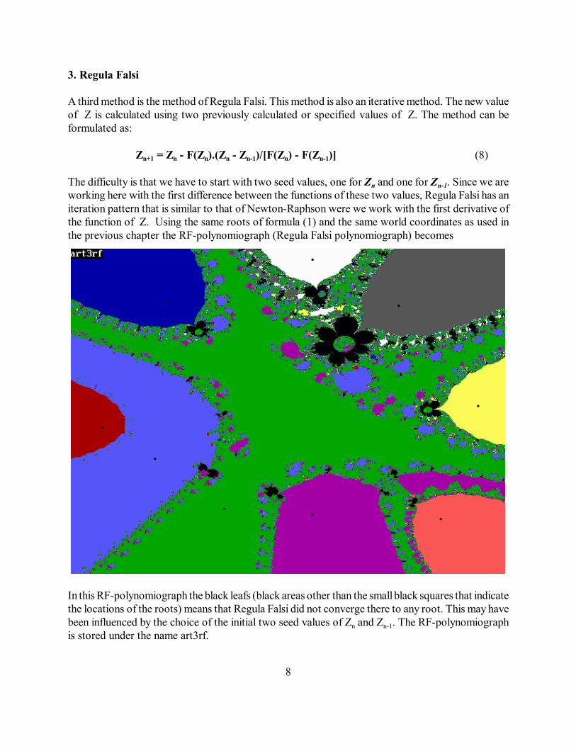
The difficulty is that we have to start with two seed values, one for Zn and one for Zn-1. Since we areworking here with the first difference between the functions of these two values, Regula Falsi has aniteration pattern that is similar to that of Newton-Raphson were we work with the first derivative ofthe function of Z. Using the same roots of formula (1) and the same world coordinates as used inthe previous chapter the RF-polynomiograph (Regula Falsi polynomiograph) becomes

In this RF-polynomiograph the black leafs (black areas other than the small black squares that indicatethe locations of the roots) means that Regula Falsi did not converge there to any root. This may havebeen influenced by the choice of the initial two seed values of Zn and Zn-1. The RF-polynomiographis stored under the name art3rf.

9

4. Extended Newton-Raphson.

In the extended Newton-Raphson method a term with the second derivative has been added to theoriginal Newton-Raphson formula and reads as follows:

Zn+1 = Zn - F(Zn)/F1(Zn) - F(Zn)2*F11(Zn)/2*F1(Zn)3 (9)

The method is applied to the equation of formula (1). In a real/imaginary window of coordinatesdefined by (-1, 1, 1, -1) (rmin, rmax, imax, imin) and a screen of 640x480 pixels all 9 roots werefound. The roots are placed in the storage address rtxx, and the visual representation in art3xx. Theroots are the same as the roots shown on page 6, but have not been calculated in the same order asthe roots found with the normal Newton-Raphson method.

The NRX-polynomiograph (Newton-Raphson eXtended polynomiograph) is shown below. The rootsare the same as roots 1, 2, 3, 5 and 8 on page 6 and their location is shown in the NRX-polynomiograph as little sqaure black dots. The larger black areas are areas of seed values with whichno roots were determined..

10

5. Other methods and conclusions.

Amongst other methods that we have not investigated (due to their complexity) are those ofBairstow, Graeffe, and the QD-method (Quotient-Difference method). Bairstow�s method dividesthe original formula by a quadratic equation, determines corrections to the result and expands this inTaylor series. The Q-D method, constructed by Stiefel, Rutishauser, and Henrici, can be used for thedetermination of eigen values of matrices and finding roots. The method is based on constructing arhombic pattern of numbers, using the higher order differences between those numbers, and solvinga set of two equations. The method of Muller is based on determining three points on the curve ofthe equation and constructing a parabola through those points. This method is discussed in chapter7. We are dealing here with choosing three points, whereas in Regula Falsi two points would besufficient for finding the roots of the equation.The convergence exponents of the methods with the exception of Bairstow�s method and the Q-Dmethod are:

1. Successive substitution: 12. Regula Falsi 1.623. Muller 1.844. Newton-Raphson 25. Newton-Raphson extended 3

The easiest of these methods is the first. However, as we have demonstrated, it is difficult to find allthe roots. In my used examples this method only found one root of a nine-degree complex equation.Methods 2 and 3 needs initial values of resp. 2 and 3 points, while for methods 4 and 5 resp. the firstderivative, and the first and second derivative have to be determined.It turns out that the fastest method is slowed down by having to calculate a complicated third termthat involves a multiplication and a division using the original function, its first and second derivative.As shown, it determines not all the roots that we want to find. The Regula Falsi method will find allthe roots, is slightly slower than Newton-Raphson, but generates RF-polynomiographs with areas inwhich roots can�t be found (black areas). This also happens with the Newton-Raphson method butless frequently. I am convinced that in most cases it finds all the roots and generates complete NR-polynomiographs, no matter whether the initial or seed values are extremely large or extremely small.In case Newton-Raphson fails, the modified method (7a) will do the trick, provided that a suitablevalue for the relaxation factor D is used. We have tried this method with world coordinates of (-100000, 100000, 100000, -100000) (rmin, rmax, imax, imin). The convergence process slows downthe larger these coordinates becomes, but it will converge to the correct roots and creates completeNR-polynomiographs. The smallest coordinates used cover an area that is 10-26 smaller than thesmallest area that contains the roots. We might have been able to try even smaller areas, where it notthat the hardware of my computer does not support the use of values that define such small areas. ______________________________________________________________________________Conjecture 2: For any given seed value, excluding the one that coincides with the origin,the method of Newton-Raphson or the modified Newton-Raphson method will find a root.______________________________________________________________________________

11

______________________________________________________________________________Conjecture 3: All roots of a complex polynomial can be found with the method of Newton-Raphson or the modified Newton-Raphson method, provided that enough seed values andan appropriate value for the relaxation value are used.______________________________________________________________________________

It is argued in the literature that the iterations in the basic Newton-Raphson method could cycle.If this happens it can be resolved by using the modified version of Newton-Raphson. Anotherproblem is the fact that the first derivative of the formula representing the NR-method canbecome zero. In my programs I have managed to stay clear of this situation.As mentioned, a large number of polynomial equations were investigated. The following chapter:Example, shows the results of one of them. From all these calculations it becomes clear that therethe highest order leafs (represented in the polynomiographs with the symbolic names ga05aa andga0500) are open leafs. That means that they will continue to infinity and have boundaries thatcan be viewed as two diverging straight lines. Note that these lines contain infinite sets of lower-order leafs. The open highest-order leafs also contain the roots associated with these leafs. Alllower-order leafs have closed boundaries. Note that each closed leaf is surrounded by a barrier ofleafs with an order that is one level lower than the leaf within this barrier. Investigations showthat these boundaries serve as barriers. If one wants to move from one leaf to the next adjacentone with very small steps, one enters such a barrier that acts as a minefield. Jumping over thisbarrier is the only way to move from the set of loci associated with one particular root to the setof loci of another root, where this second set of loci has the appearance of being a directneighbour of the first set of loci. These barriers consist basically of a chain of a bundle of leafs andin which these leafs represent the leafs associated with the roots of the original equation (1).Whether we defined the real/imaginary coordinates extremely large or extremely small, thispattern of open and closed leafs will reappear, as shown in the example of the next paragraph. Theonly handicap in this process is the limited way in which real numbers can be represented with ourcomputer equipment. All the performed calculations shows polynomiographs of which we havedrawn the following conclusions:

______________________________________________________________________________

Conjecture 4: An NR-polynomiograph consists of open leafs in which the roots of apolynomial equation are located, and an infinitely large amount of closed leafs. ______________________________________________________________________________

______________________________________________________________________________

Conjecture 5: Leafs of the same order are separated from each other by a barrier of leafs ofa lower order. No two leafs of the same order are directly adjacent to each other.______________________________________________________________________________

12

6. Example.

Consider the equation C Zmm

mm

=

=

∑ =0

9

0

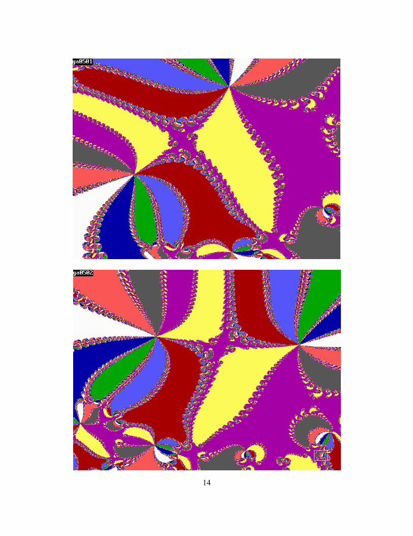
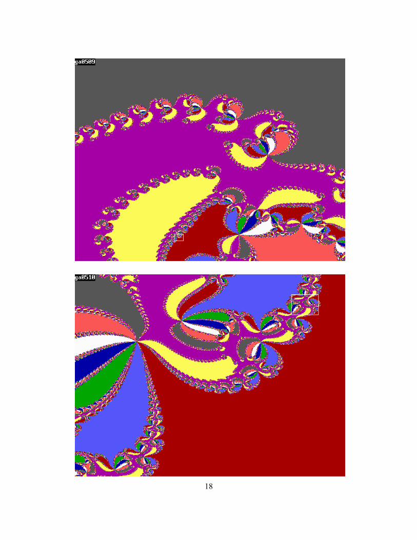
where C0 = 4 + 6.i; C1 = .3 - 1.i; C2 = .8 - .5.i; C3 = -.25 + .5 .i; C4 = .5 + .5.i; C5 = .7 - .75.i; C6 = -.35 + .75.i; C7 = .45 - .25.i; C8 = -.65 + .25.i; C9 = 1 The roots are (calculated with an accuracy of 0.0001): Root1: -.8606220286249983 + .6659487704078041*i (blue) Root2: -.3260056834276752 + 1.283126586328105 *i (green) Root3: .5992787509712372 + 1.103682709656271*i (light blue) Root4: 1.1734550366744960 + .5590327452828046*i (red) Root5: .8245803640955177 - .9748311601773331*i (magenta) Root6: 1.2101329495036600 - .4380346718883291*i (yellow) Root7: -1.1452672657445820 - .2252986466412862 *i (white) Root8: .0247114547197130 - 1.203766313565029 *i (gray) Root9: -.8502635781658199 - 1.019860019403639 *i (light red) We have generated various NR-polynomiographs with the following with windows defined by thefollowing world coordinates (rmin, rmax, imax, imin):

ga05aa: -100, 100, 100, -100ga0500: -1.3 1.3, 1.3 -1.3 (here the locations of the roots are identified with small black squares)ga0501: -1.04, -.78, .26,0ga0502: -1.027, -1.014,0.013,0ga0503: -1.0153,-1.01465,0.0013,0.00065ga0504: -1.014745,-1.014715,0.0009,0.00087ga0505: -1.014718,-1.014715,0.000876,0.000873ga0506: -1.01471635,-1.01471620,0.00087510,0.00087495ga0507: -1.01471632,-1.014716305,0.00087501,0.000874995ga0508: -1.014716308, -1.0147163075, 0.0008750085, 0.000875008ga0509: -1.0147163079, -1.0147163076, 0.0008750085, 0.0008750082ga0510: -1.01471630779; -1.01471630778, 0.00087500824, 0.00087500823ga0511: -1.014716307782, -1.014716307781, 0.000875008239, 0.000875008238

Note that the surface of the largest polynomiograph (ga05aa) is 40,000 units and the surface ofthe smallest polynomiograph (ga0510) is 10-24 units.

13

14

15

16

17

18

19

This is one of the smallest polynomiograph I was able to generate. Polynomiographs that are 10%smaller tend to become irregular due to the loss of significance in the presentation of floatingpoint numbers. I am convinced that with more powerful machines and/or computers of which therepresentation of floating point numbers are more accurate will be able to generate ad infinitumthe same kind of patterns. Observations

1. With the previously described methods certain problems may arise. That is especially the case ifa complex polynomial has one or more roots that are identical. With our root-finding approach wewill miss those roots, despite the fact that we are using all the seed values that are associated withthe pixel values of the display screen.If, using the Newton-Raphson method, we find a number of roots that is smaller than the degreeof the polynomial, it is quite certain that we are dealing with identical roots. To find these rootswe can apply the following strategy.Assume that the degree of the polynomial is n and that we find k roots (k<n) We will divide theoriginal polynomial by a polynomial of the form (Z-Z1).(Z-Z2)......(Z-Zk). The newly generatedpolynomial is of the order m = n-k and of the form:

20

(10)F Z C Z Z Znew jj

j nj

ii

i k

( ) / ( )= −=

=

=

=

∑ ∏0 1

If m = 2 or 3 we can easily solve the new equation with analytical means. It means we are dealingwith 2 or 3 roots that have identical values. If m is larger than 3 we have to solve the roots of thisnew function in the same way as we did with the original polynomial.

2. One must be careful with the definition of the frame within which one tries to determine theroots. It is possible to define that frame too small resulting in covering an area in a leaf that willdetermine the root associated to that leaf only.

3. Once a seed value has been selected that is located in a specific closed leaf of any order (otherthan the highest order) , the iteration process will determine new starting values that will alwaysbe located in leafs (probably of different order) that belong to the same class of leaves or stateddifferently: leafs that are associated with the same root. The process jumps from leaf to leaf whereall these leafs have the same colour. It ends when values are found in the highest-order open leafand the process will iterate to the root associated with this leaf.

21

7. Muller�s method.

This is the most elaborate of all the methods that I investigated with the objective of finding the rootsof high degree complex polynomials and generating polynomiographs of the results. In Muller�smethod we have to determine the roots of:

F(Z,C) = ; C and Z are complex numbers; degree of polynomial is kC Znn

n kn

=

=

∑0

and apply this method by defining a quadratic curve through three points on the curve defined by thecomplex polynomial function F(Z) and intersecting this curve with the X-axis. This leads to theequation:

(11)

( ).( )( ).( )

* ( )( ).( )

( ).( )* ( )

( ).( )( ).( )

* ( )

Z Z Z ZZ Z Z Z

F ZZ Z Z Z

Z Z Z ZF Z

Z Z Z ZZ Z Z Z

F Z

n n

n n n nn

n n

n n n nn

n n

n n n nn

− −− −

+− −− −

+

+− −− −

=

− −

− −

−

− − −−

−

− − −−

2 1

2 1

2

1 2 11

1

2 1 22 0

The values of Z are calculated by assigning world coordinates for complex numbers to the screencoordinates (640x480) in the same way as we did in the case of the previous methods. In this waywe examine all 640x480 seed values for Zn. The values of Zn-1 and Zn-2 are derived from Zn by makingthem slightly different from Zn.This quadratic equation results in two values for Z, which is the new seed value in the iterationprocess for finding one of the roots of the polynomial. We chose one of these values by comparingthem to the lastly found Z and continue with the value which is closest to that lastly found value. Incase we don�t find all the roots we will repeat the iteration process, starting from the initially chosenseed value(s) and pick the Z value which is the result of applying the positive sign in the quadraticequation (11). We can exhaust the search for all the roots by repeating the iteration process oncemore and choosing the other sign of the quadratic equation.

With Muller�s method we have found the roots of formula (1) with C = -.37-.63i, and using worldcoordinates between (-1.2, 1.2, 1.2, -1.2) for resp. rmin, rmax, imax, imin. As expected, the roots aresimilar to those found with Newton-Raphson or Regula Falsi.The generated polynomiograph (MU-polynomiograph) is totally different from the NR-polynomiograph and RF-polynomiograph. The boundaries between the coloured areas are sharp andthe picture exhibits a rather chaotic character. Many seed values did not result in finding any root (theblack areas in the MU-polynomiograph with the symbolic name gmul1). This may have been causedby the limit that was set in the number of allowed iteration steps. It is also possible that the usedstrategies where we had to make a choice in determining which value of the two values that are theresult of evaluating formula (11) had to be used. A random selection of the use of the plus- or minus-sign in calculating Z in formula (11) might give different results. Due to the complication of makingthese choices the time necessary for generating the MU-polynomiograph is extremely long. However,

22

the program that calculates the roots is almost as fast as the program used in the Newton-Raphsonapproach, despite the more elaborate computations that are involved in Muller�s method.

The MU-polynomiograph for the complex equation of formula (1) is shown below. The little blacksquare boxes in the larger coloured patterns indicate the location of the roots.