fractal geometry and superformula to model natural shapes

IJRRAS 16 (4) ● October 2013 www.arpapress.com/Volumes/Vol16Issue4/IJRRAS_16_4_09.pdf

78

FRACTAL GEOMETRY AND SUPERFORMULA TO MODEL NATURAL

SHAPES

Nicoletta Sala

Università della Svizzera italiana, Largo Bernasconi, CH - 6850 Mendrisio, Switzerland

ABSTRACT

Mathematics is a branch of the science which has been used to model the natural and the biological forms, for many

centuries. Pythagoras, Aristotle, Fibonacci, Cardano, Bernoulli, Euler, Laplace, Gauss, von Helmholtz, Riemann, Einstein,

Thompson, Turing, Wiener, von Neumann, Keller, and others studied important applications of mathematics to life

sciences and significant developments in mathematics motivated by the life sciences.

Euclidean geometry, which dominated our mathematical thinking for centuries, has lost importance, because its

primitive concepts (point, straight line and surface) and its simple constructs (squares and triangles) do not find

application in the description of the natural objects.

Plato was able to reconcile the inability of classical geometry (as later formulated by Euclid) to describe the world

we inhabit, and more recently, Mandelbrot has argued that fractal geometry could provide a coherent description of

the design principles underlying living organisms.

This paper presents the fractal geometry, with its properties and its characteristics, as a useful tool to describe and to

study the natural forms (e.g., fern, trees, seashells, bushes, basins of rivers, mountains), and the “superformula” by

Gielies to model many complex shapes and curves that are found in nature. Keywords: Box-counting Dimension, Fractal Dimension, Fractal Geometry, Iterated Function Systems, L-Systems,

Natural Shapes, Self-Similarity, Superformula.

1. INTRODUCTION

First studies on fractals were at the beginning of the 20th

century by French mathematicians Pierre Fatou (1878-

1929) and Gaston Julia (1893-1978). Only in the second part of the same century, the Polish-born Franco-American

Benoit Mandelbrot (1924-2011) coined the word “Fractal”. It derives from the Latin verb “frangere”, “to break”,

and from the related adjective “fractus”, “fragmented and irregular”. This term denotes the geometry of nature,

which traces inherent order in chaotic shapes and processes, and it was created to differentiate pure geometric

figures from other types of figures that defy such simple classification. It also characterizes spatial or temporal

phenomena that are continuous but not differentiable.

Mandelbrot (1989) defined fractal geometry as : “a workable geometric middle ground between ground between the

excessive geometric order of Euclid and geometric chaos of general mathematics… Fractal geometry is

conveniently viewed as a language that has proven its value by its uses” [1].

The acceptance of the word “fractal” was dated in 1975, when Mandelbrot presented the list of publications between

1951 and 1975, date when the French version of his book was published, although Mandelbrot‟s famous seminal

paper on fractal dimension and statistical self-similarity dates back to 1967. After this book, the people were

surprised by the variety of the studied fields: economy, linguistics, cosmology, noise on telephone lines, turbulence

[2].

Fractal geometry replaces Euclidian geometry and it is recognized as the true geometry able to describe the Nature.

Recently, the electronics evolution and the increase in the computer calculation power permitted connections

between the fractal geometry and the other disciplines (for example, biology, economy, medicine, engineering, arts,

architecture, computer science, industrial design), and the multiplicity of applications had an important role in the

diffusion of fractal geometry [3, 4, 5, 6, 7, 8, 9].

This paper, which describes the application of fractal geometry to model natural shapes, is organized as follows:

section 2 introduces the fractal objects, section 3 presents the applications of the fractal geometry to model natural

forms. Section 4 describes Gielies‟ Superformula, and the section 5 is dedicated to the conclusions.

2. FRACTAL OBJECTS

A fractal object could be defined as a fragmented geometric shape that can be subdivided in parts, each of which is

approximately a reduced-size copy of the whole [3].

Fractal objects and processes are said to display „self-invariant‟ (self-similar or self-affine) properties [10].

IJRRAS 16 (4) ● October 2013 Sala ● Superformula to Model Natural Shapes

79

Fractals are generally self-similar on multiple scales. So, all fractals have a built-in form of iteration or recursion.

Sometimes the recursion is visible in how the fractal is constructed. For example, Koch snowflake (figure 1a),

Cantor set, and the Sierpinski triangle are all generated using simple recursive rules. Self similarity is present in

nature, too. Figures 1b shows a natural fractal object, the cauliflower which has the property of self similarity (it

repeats its shape in different scales).

a) b)

Figure 1. Koch snowflake is a fractal generated using simple geometric rules a).

The cauliflower is a fractal present in the nature b)

Excellent summaries of basic concepts of fractal geometry can be found in Mandelbrot [1, 3], Schroeder [11],

Turcotte [12], Hastings and Sugihara [10], Briggs [13].

3. FRACTAL GEOMETRY TO MODEL NATURAL SHAPES

Fractal properties include self-similarity and infinite length. In fractal analysis, the Euclidean concept of „length‟ is

conceived as a process. This process is characterized by a constant parameter D known as the fractal (or fractional)

dimension.

3.1 The self-similarity

The invariance against changes in scale or size is named “self-similarity”, and it is a property by which an object

contains smaller copies of itself at arbitrary scales. Mandelbrot defined the self-similarity as follow: “When each

piece of a shape is geometrically similar to the whole, both the shape and the cascade that generate it are called self-

similar” [3]. “Similar” means that the relative proportions of the internal angles and shapes‟ sides remain the same.

Mandelbrot used the term “self-similar” for the first time in 1964, in an internal report at IBM, where he was doing

research, and in the title of a 1965 paper. A fractal object is self-similar. This means that as viewers peer deeper into

the fractal image, we can observe that the shapes seen at one scale are similar to the shapes seen in the detail at

another scale.

There are three kinds of self-similarity:

Exact self-similarity. The fractal is identical at different scales. This is the strongest kind of self-similarity.

Quasi-self-similarity. The fractal is approximately (but not in exact way) identical at different scales. This is a

less precise form of self-similarity. Quasi-self-similar fractals contain small copies of the entire fractal in

degenerate and distorted shapes. This is the kind of fractals defined by recurrence relations.

Statistical self-similarity. The fractal has statistical or numerical measures which are preserved across scales;

instead of specifying exact scales, at each iteration the scale of each piece is selected randomly from a set range.

This is the weakest kind of self-similarity. Most common definitions of “fractal” imply this kind of self-

similarity. Random fractals are examples of fractals which are statistically self-similar.

Mandelbrot (1982) observed that self-similarity is ubiquitous in the natural world, and in the human body is possible

to observe the presence of fractal geometry using two different points of view: temporal fractals and spatial fractals

[3]. Temporal fractals are present in some dynamic processes, for example in the cardiac rhythm. In fact, heart rates

show chaotic and self-similar patterns (as shown in figure 2) . This is not because of physical reasons, as many


80

might believe, but because of physiological reasons [14]. Another interesting consideration is connected to the

complexity of the graph of the heart rate. A graph of a healthy heart has more complexity then a diseased heart, for

example with congestive heart failure (CHF) (as shown in figure 3).

Chaotic property the complexity is associated to the healthy in many physiological aspects [15].

Figure 2. Heart rates show chaotic and self-similar patterns


81

Figure 3. The top heart rate time series is from a healthy subject; bottom left is from a subject with heart failure,

and bottom right from a subject with atrial fibrillation

Spatial fractals refer to the presence of self-similarity observed to various enlargements, for instance, the small

intestine repeats its form on different scales. Spatial fractals also refer to the branched patterns that are present inside

the human body for enlarging the available surface for the absorption of the substances, and the distribution and the

collection of the solutes occupying a relative small fraction of the body. The lungs are an excellent example of a

natural fractal organ, they have the branching pattern as the trees. [16]

Figure 4a shows the frontal view of dog‟s lungs. It is an example of self-similarity in the nature. In figure 4b there is

an example of a fractal object which represents an attempt to reproduce complex shapes of the lungs, using few

simple geometric rules.

Figure 5 shows a cast of human airway tree (a) compared with Koch tree model for airways (b) [17].

Fractal patterns are recognised at various spatial scales, as shown in figure 6.


82

Fractal geometry could be a unifying theme in biology, it permits a generalization of the concepts of dimension and

length measurement [18].

a) b)

Figure 4. Frontal view of dog’s lungs a) it is a natural fractal object. “Fractal lungs” b) is a fractal generated

using simple geometric rules, starting from two triangles.

Figure 5. Cast of human airway tree (a) compared with Koch tree model for airways (b) [17]


83

Figure 6. Fractal patterns are observed various spatial scales. The ovals are general processes operating at each

scale: biotic processes predominate at inner spatial scales, abiotic processes at coarser scales. Rectangles

represent the scientific disciplines [18].

3.2 Fractal dimension

Euclidean geometric forms are regular and have integer dimensions (1, 2, and 3, for line, surface, and volume

respectively). A fractal line has a dimension between 1 and 2. Fractal dimension characterizes fractal sets and fractal

patterns by quantifying their complexity as a ratio of the change in detail to the change in scale [19].

The basic idea of a "fractured" dimension has been described by Benoit Mandelbrot in his 1967 paper on self-

similarity, where he cited a previous work written by English mathematician and meteorologist Lewis Fry

Richardson (1881-1953) describing the counter-intuitive notion that a coastline's measured length changes with the

length of the measuring ruler used. The estimated length, L, equals the length of the ruler, s, multiplied by the N, the

number of such rulers needed to cover the measured object.

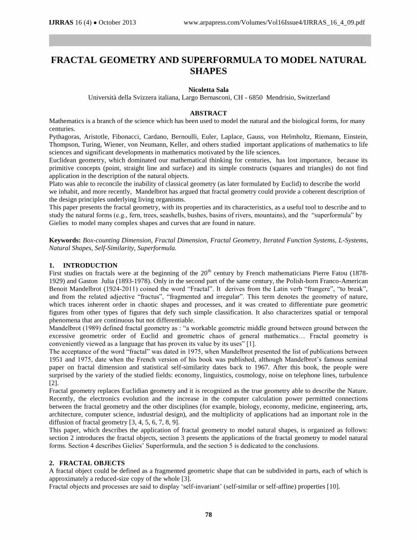
Richardson demonstrated that the measured length of coastlines appears to increase without limit as the unit of

measurement is made smaller.

This is called “Richardson effect” (also known as “Coastlines Paradox”): the length of the coast of Britain depends

on the scale of measurement [19] (figure 7).

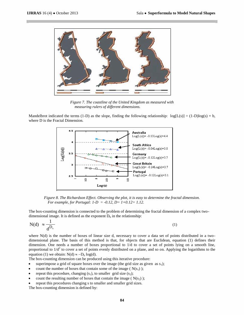
Richardson pointed out his attention on the regularity between the length of national boundaries, and coastlines, and

the scale size; observing that the relation between length estimate and length of scale is linear on a log-log plot

(Figure 8).


84

Figure 7. The coastline of the United Kingdom as measured with

measuring rulers of different dimensions.

Mandelbrot indicated the terms (1-D) as the slope, finding the following relationship: log[L(s)] = (1-D)log(s) + b,

where D is the Fractal Dimension.

Figure 8. The Richardson Effect. Observing the plot, it is easy to determine the fractal dimension.

For example, for Portugal: 1-D = -0.12, D= 1+0.12= 1.12.

The box-counting dimension is connected to the problem of determining the fractal dimension of a complex two-

dimensional image. It is defined as the exponent Db in the relationship:

bD

d

1(d)N (1)

where N(d) is the number of boxes of linear size d, necessary to cover a data set of points distributed in a two-

dimensional plane. The basis of this method is that, for objects that are Euclidean, equation (1) defines their

dimension. One needs a number of boxes proportional to 1/d to cover a set of points lying on a smooth line,

proportional to 1/d2 to cover a set of points evenly distributed on a plane, and so on. Applying the logarithms to the

equation (1) we obtain: N(d) Db log(d).

The box-counting dimension can be produced using this iterative procedure:

superimpose a grid of square boxes over the image (the grid size as given as s1);

count the number of boxes that contain some of the image ( N(s1) );

repeat this procedure, changing (s1), to smaller grid size (s2);

count the resulting number of boxes that contain the image ( N(s2) );

repeat this procedures changing s to smaller and smaller grid sizes.

The box-counting dimension is defined by:


85

1

1log

2

1log

))]1

(log())2

([log(

sN

sN

sNsN

bD

...736.1log(4)][log(8)

log(27)][log(90)

1s

1Nlog

2s

1Nlog

))]1log(N(s))2[log(N(sDB

...807.1log(8)][log(16)

log(90)][log(315)

1s1

Nlog

2s1

Nlog

))]1

log(N(s))2

[log(N(sDB

(2)

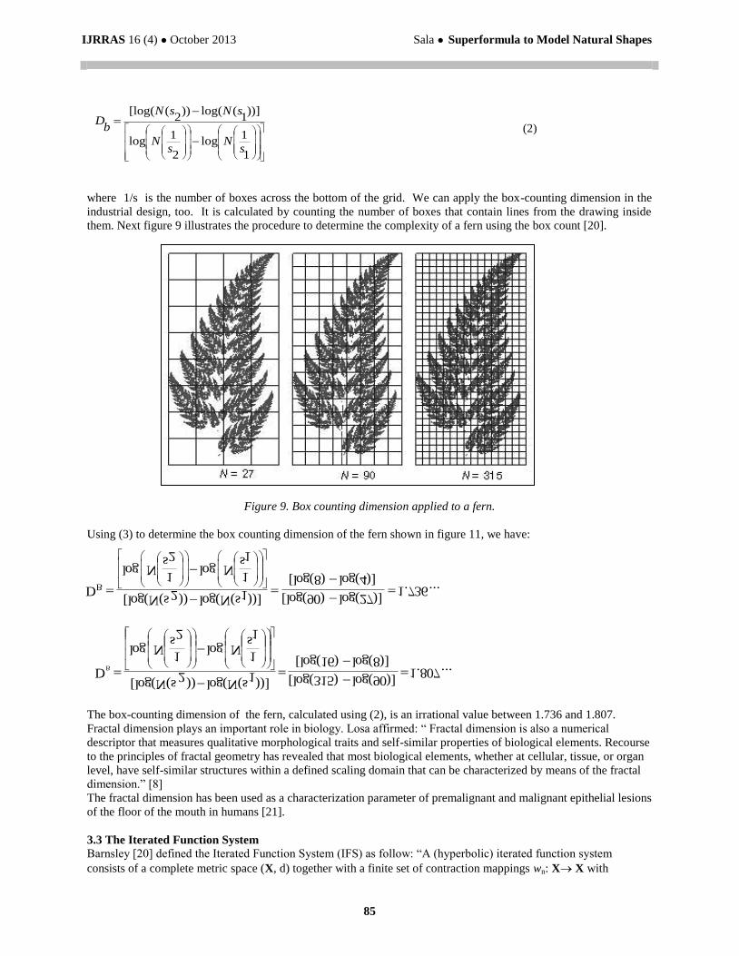
where 1/s is the number of boxes across the bottom of the grid. We can apply the box-counting dimension in the

industrial design, too. It is calculated by counting the number of boxes that contain lines from the drawing inside

them. Next figure 9 illustrates the procedure to determine the complexity of a fern using the box count [20].

Figure 9. Box counting dimension applied to a fern.

Using (3) to determine the box counting dimension of the fern shown in figure 11, we have:

The box-counting dimension of the fern, calculated using (2), is an irrational value between 1.736 and 1.807.

Fractal dimension plays an important role in biology. Losa affirmed: “ Fractal dimension is also a numerical

descriptor that measures qualitative morphological traits and self-similar properties of biological elements. Recourse

to the principles of fractal geometry has revealed that most biological elements, whether at cellular, tissue, or organ

level, have self-similar structures within a defined scaling domain that can be characterized by means of the fractal

dimension.” [8]

The fractal dimension has been used as a characterization parameter of premalignant and malignant epithelial lesions

of the floor of the mouth in humans [21].

3.3 The Iterated Function System

Barnsley [20] defined the Iterated Function System (IFS) as follow: “A (hyperbolic) iterated function system

consists of a complete metric space (X, d) together with a finite set of contraction mappings wn: X X with


86

)()( 1 AwAWA n

n

n

)()(1

BwBW nnn

))(,(

)0(1 LwLh n

n

nn

sALh

1),(

))(,()1(),()0(

1

1 LwLhsALh nn

n

respective contractivity factor sn, for n = 1, 2,.., N. The abbreviation “IFS” is used for “iterated function system”.

The notation for the IFS just announced is X, wn, n = 1, 2,.., N and its contractivity factor is s = max sn : n = 1,

2, …, N.” Barnsley put the word “hyperbolic” in parentheses because it is sometimes dropped in practice. He also

defined the following theorem : “Let X, wn, n = 1, 2, …, N be a hyperbolic iterated function system with

contractivity factor s [20]. Then the transformation W: H(X) H(X) defined by:

(3)

For all B H(X), is a contraction mapping on the complete metric space (H(X), h(d)) with contractivity factor s.

That is:

H(W(B), W(C)) sh(B,C) (4)

for all B, C H(X). Its unique fixed point, A H(X), obeys

(5)

and is given by A = lim n Won

(B) for any B H(X).”

The fixed point A H(X), described in the theorem by Barnsley is called the “attractor of the IFS” or “invariant

set”.

An affine map of the plane is given by form:

and it is determined by six number, a, b, c, d, e, and f. The affine maps are combinations of translations, rotations

and scalings in the plane. If the scaling factor is less than 1, we have contractive affine maps.

Bogomolny (1998) affirms that two problems arise. One is to determine the fixed point of a given IFS, and it is

solved by what is known as the “deterministic algorithm”.

The second problem is the inverse of the first: for a given set AH(X), find an iterated function system that has A as

its fixed point [22]. This is solved approximately by the Collage Theorem [20].

The Collage Theorem states: “Let (X, d), be a complete metric space. Let LH(X) be given, and let o be given.

Choose an IFS (or IFS with condensation) X, (wn), w1, w2,…, wn with contractivity factor 0 s 1, so that

(6)

Where h(d) is the Hausdorff metric. Then

(7)

Where A is the attractor of the IFS. Equivalently,

(8)

for all LH(X).”

The Collage Theorem describes how to find an Iterated Function System whose attractor is “close to” a given set,

one must endeavour to find a set of transformations such that the union, or collage, of the images of the given set

under transformations is near to the given set.

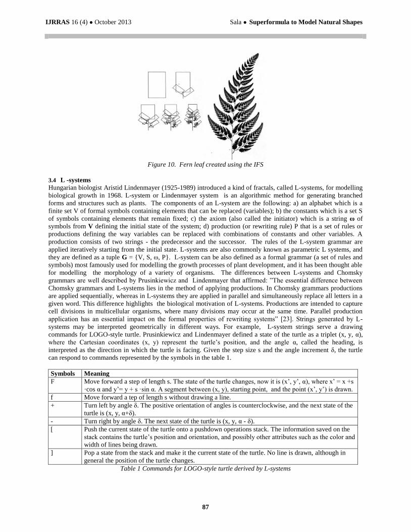
The IFS is produced by polygons, in this case: squares, that are put in one another. The final step of this iterative

process shows a fern which has high degree of similarity to real one (figure 10).

f

e

y

x

db

ca

y

xw


87

Figure 10. Fern leaf created using the IFS

3.4 L -systems

Hungarian biologist Aristid Lindenmayer (1925-1989) introduced a kind of fractals, called L-systems, for modelling

biological growth in 1968. L-system or Lindenmayer system is an algorithmic method for generating branched

forms and structures such as plants. The components of an L-system are the following: a) an alphabet which is a

finite set V of formal symbols containing elements that can be replaced (variables); b) the constants which is a set S

of symbols containing elements that remain fixed; c) the axiom (also called the initiator) which is a string ω of

symbols from V defining the initial state of the system; d) production (or rewriting rule) P that is a set of rules or

productions defining the way variables can be replaced with combinations of constants and other variables. A

production consists of two strings - the predecessor and the successor. The rules of the L-system grammar are

applied iteratively starting from the initial state. L-systems are also commonly known as parametric L systems, and

they are defined as a tuple G = {V, S, ω, P}. L-system can be also defined as a formal grammar (a set of rules and

symbols) most famously used for modelling the growth processes of plant development, and it has been thought able

for modelling the morphology of a variety of organisms. The differences between L-systems and Chomsky

grammars are well described by Prusinkiewicz and Lindenmayer that affirmed: ”The essential difference between

Chomsky grammars and L-systems lies in the method of applying productions. In Chomsky grammars productions

are applied sequentially, whereas in L-systems they are applied in parallel and simultaneously replace all letters in a

given word. This difference highlights the biological motivation of L-systems. Productions are intended to capture

cell divisions in multicellular organisms, where many divisions may occur at the same time. Parallel production

application has an essential impact on the formal properties of rewriting systems” [23]. Strings generated by L-

systems may be interpreted geometrically in different ways. For example, L-system strings serve a drawing

commands for LOGO-style turtle. Prusinkiewicz and Lindenmayer defined a state of the turtle as a triplet (x, y, α),

where the Cartesian coordinates (x, y) represent the turtle‟s position, and the angle α, called the heading, is

interpreted as the direction in which the turtle is facing. Given the step size s and the angle increment δ, the turtle

can respond to commands represented by the symbols in the table 1.

Symbols Meaning

F Move forward a step of length s. The state of the turtle changes, now it is (x‟, y‟, α), where x‟ = x +s

·cos α and y‟= y + s ·sin α. A segment between (x, y), starting point, and the point (x‟, y‟) is drawn.

f Move forward a tep of length s without drawing a line.

+ Turn left by angle δ. The positive orientation of angles is counterclockwise, and the next state of the

turtle is (x, y, α+δ).

- Turn right by angle δ. The next state of the turtle is (x, y, α - δ).

[ Push the current state of the turtle onto a pushdown operations stack. The information saved on the

stack contains the turtle‟s position and orientation, and possibly other attributes such as the color and

width of lines being drawn.

] Pop a state from the stack and make it the current state of the turtle. No line is drawn, although in

general the position of the turtle changes.

Table 1 Commands for LOGO-style turtle derived by L-systems


88

Originally the L-systems were devised to provide a formal description of the development of such simple

multicellular organisms, and to illustrate the neighbourhood relationships between plant cells. Later on, this system

was extended to describe higher plants and complex branching structures. Smith (1984) was the first to prove that L-

systems were useful in computer graphics for describing the structure of certain plants, in his paper: “Plants,

Fractals, and Formal Languages” [24]. He described that these objects should not be labeled as “fractals” for their

similarity to fractals, introducing a new class of objects which Smith called “graftals”. This class had of great

interest in the Computer Imagery [24, 25]. Figure 11a shows an example of plant-like structures generated after five

iterations by bracketed L-systems with the initial string F (angle = 20°), and the replacement rule F F[+F] F[-F]

[F]. In figure 11b there is a plant-like structures generated after four iterations by bracketed L-systems with the

initial string F (angle = 22.5°), and the replacement rule F FF+[+F-F-F] -[-F+F+F].

a) b)

Figure 11. Plant-like structures generated by bracketed L-systems with five (a) and four iterations (b)

3.5 Fractal geometry and landscapes

Other interesting application of fractal geometry is to model landscapes which include terrain, mountains, trees.

Fournier et al. [26] developed a mechanism for generating a kind of fractal mountains based on recursive

subdivision algorithm for a triangle. Here, the midpoints of each side of the triangle are connected, creating four new

subtriangles. Figure 12 shows the subdivision of the triangle into four smaller triangle, figure 12b illustrates how the

midpoints of the original triangle are perturbed in the y direction [25]. To perturb these points, can be use the

properties of the self-similarity, and the conditional expectation properties of fractional Brownian motion

(abbreviated to fBm).

The fractional Brownian motion was originally introduced by Mandelbrot and Van Ness in 1968 as a generalization

of the Brownian motion (Bm). FBm basically consists of steps in a random direction and with a step-length that has

some characteristic value. Hence the random walk process. An important feature of fBm is the self-similarity (if we

zoom in on any part of the function we will produce a similar random walk in the zoomed in part). Other polygons

can be used to generate the grid (e.g., triangles and hexagons).


89

a) b)

Figure 12. The subdivision of a triangle into four smaller triangle a). Perturbation in the y direction of the

midpoints of the original triangle b)

This method evidences two problems, which are classified as internal and external consistency problems [26].

Internal consistency is the reproducibility of the primitive at any position in an appropriate coordinate space and at

any level of detail, so the final shape is independent of the orientation of the subdivided triangle. This is satisfied by

a Gaussian random number generator which depends on the point‟s position, thus it generates the same numbers in

the same order at a given subdivision level. The external consistency concerns the midpoint displacement at shared

edges and their direction of displacement.

This process, when iterated, produces a deformed grid which represents a surface, an example is shown in figure 13.

After the rendering phase (that includes: hidden line, coloured, and shaded) can appear a realistic fractal mountain,

as shown in figure 14.

Figure 13. Grid of squares generated by a recursive subdivision and applying the fractional Brownian motion


90

Figure 14. Fractal mountains

These examples describe how to realize fractal mountains but not their erosion. Musgrave et al. [27] introduced

techniques which are independent of the terrain creation. The algorithm can be applied to already generated data

represented as regular height fields require separate processes to define the mountain and the river system.

Prusinkiewicz and Hammel [28] combined the midpoint-displacement method for mountain generation with the

squig-curve model of a non-branching river originated by Mandelbrot [29]. Their method created one non-branching

river as result of context sensitive L-system operating on geometric objects (a set of triangles). Three key problems

remained open (i) the river flowed at a constant altitude, (ii) the river flowed in an asymmetric valley, and (iii) the

river had no tributaries. Figure 15 shows an example of a squig-curve construction (recursion levels 0–7) [28]

Figure 15. Squid-curve construction (recursion level 0-7)

Maràk et al [30] reported a method for synthetical terrain erosion, that is based on rewriting process of matrices

representing terrain parts, which were rewritten using certain user-defined set of rules which represented an erosion

process. The method consisted in three kinds of rewriting process [30].

4. The “Superformula”

Belgian biologist Johan Gielies has introduced, in his report A generic geometric transformation that unifies a wide

range of natural and abstract shapes (2003), a geometrical approach for modeling and understanding various

natural shapes [31]. He started from the concept of the circle, showing that a large variety of shapes can be

described by a single and simple geometrical equation, that he has called the Superformula:


91

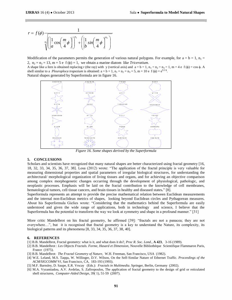
Modification of the parameters permits the generation of various natural polygons. For example, for a = b = 1, n1 =

2, n2 = n3 = 13, m = 5 e f () = 1, we obtain a marine diatom like Triceratium. A shape like a fern is obtained replacing r (the ray) with y (vertical axis) and a = b = 1, n1 = n2 = n3 = 1, m = 4 e f () = cos . A

shell similar to a Pleuroploca trapezium is obtained: a = b = 1, n1 = n2 = n3 = 5, m = 10 e f () = e0,2 .

Natural shapes generated by Superformula are in figure 16.

Figure 16. Some shapes derived by the Superformula

5. CONCLUSIONS

Scholars and scientists have recognized that many natural shapes are better characterized using fractal geometry [16,

18, 32, 33, 34, 35, 36, 37, 38]. Losa (2012) wrote: “The application of the fractal principle is very valuable for

measuring dimensional properties and spatial parameters of irregular biological structures, for understanding the

architectural/ morphological organization of living tissues and organs, and for achieving an objective comparison

among complex morphogenetic changes occurring through the development of physiological, pathologic, and

neoplastic processes. Emphasis will be laid on the fractal contribution to the knowledge of cell membranes,

hematological tumors, cell tissue cancers, and brain tissues in healthy and diseased states.” [8].

Superformula represents an attempt to provide the precise mathematical relation between Euclidean measurements

and the internal non-Euclidean metrics of shapes, looking beyond Euclidean circles and Pythagorean measures.

About his Superformula Gielies wrote: “Considering that the mathematics behind the Superformula are easily

understood and given the wide range of applications, both in technology and science, I believe that the

Superformula has the potential to transform the way we look at symmetry and shape in a profound manner.” [31]

More critic Mandelbrot on his fractal geometry, he affirmed [39]: “fractals are not a panacea; they are not

everywhere…”, but it is recognised that fractal geometry is a key to understand the Nature, its complexity, its

biological patterns and its phenomena [8, 33, 34, 35, 36, 37, 38, 40].

6. REFERENCES [1] B.B. Mandelbrot, Fractal geometry: what is it, and what does it do?, Proc R. Soc. Lond., A 423, 3-16 (1989).

[2] B.B. Mandelbrot : Les Objects Fractals. Forme, Hasard et Dimension, Nouvelle Bibliothèque Scientifique Flammaron Paris,

France (1975).

[3] B.B. Mandelbrot: The Fractal Geometry of Nature, W.H. Freeman, San Francisco, USA (1982).

[4] W.E. Leland, M.S. Taqqu, W. Willinger, D.V. Wilson, On the Self-Similar Nature of Ethernet Traffic. Proceedings of the

ACM/SIGCOMM’93, San Francisco, CA, 183-193 (1993).

[5] M.F. Barnsley, D. Saupe, E.R. Vrscay (Eds.): Fractals in Multimedia. Springer, Berlin, Germany (2002).

[6] M.A. Vyzantiadou, A.V. Avdelas, S. Zafiropoulos, The application of fractal geometry to the design of grid or reticulated

shell structures, Computer-Aided Design, 39( 1), 51-59 (2007).

1

32

4

1

4cos

1

1)(

n

nn

msin

b

m

a

fr


92

[7] M. Ostwald: Fractal Architecture: Knowledge formation within and between architecture and the sciences of complexity,

VDM Verlag, Saarbrücken, Germany (2009).

[8] G.A.Losa, Fractals and their contribution to biology and medicine, Medicographia, 30(3), 365-374 (2012).

[9] N. Sala, Fractals, Computer Science and Beyond, F. Orsucci, N. Sala (eds): Complexity Science, Living Systems, and

Reflexing Interfaces: New Models and Perspectives, IGI Global, Hershey, USA (2013).

[10] H.M. Hastings, G. Sugihara: Fractals: a user’s guide for the natural sciences. Oxford University Press, Oxford, England

(1993).

[11] M. Schroeder: Fractals, chaos, power laws. Minutes from an infinite paradise, Freeman, New York, USA (1991).

[12] D.L. Turcotte: Fractals and chaos in geology and geophysics, Cambridge University Press, Cambridge, England (1992).

[13] J. Briggs: Fractals: The Patterns of Chaos: Discovering a New Aesthetic of Art, Science, and Nature, Simon & Schuster,

New York, USA (1992).

[14] A.L. Goldberger, L.A.N. Amaral, L. Glass, J.M. Hausdorff, P.Ch. Ivanov, R.G. Mark, J. E. Mietus, G.B.Moody, C-K. Peng,

H.E. Stanley. PhysioBank, PhysioToolkit, and PhysioNet: Components of a New Research Resource for Complex

Physiologic Signals. Circulation 101(23), e215-e220 [Circulation Electronic Pages;

http://circ.ahajournals.org/cgi/content/full/101/23/e215] (2000).

[15] A.L. Goldberger, L.A.N. Amaral, J.M. Hausdorff, P. Ch. Ivanov, C.-K. Peng, H. Eugene Stanley, Fractal dynamics in

physiology: Alterations with disease and aging, Proc. Natl. Acad. Sci. USA, 99 (suppl_1), 2466-2472 (2002).

[16] S. Havlin, S.V. Buldyrev, A.L. Goldberger, R.N. Mantegna, S.M. Ossadnik, C.K. Peng, M. Simons, H.E. Stanley, Fractals

in biology and medicine, Chaos Solitons Fractals, 6,171-201 (1995).

[17] E.R. Weibel, Mandelbrot‟s Fractals and the Geometry of Life: A Tributeto Benoit Mandelbrot on his 8oth Birthday, G.A.

Losa, D. Merlini, T.F. Nonnenmacher, E.R. Weibel (eds.): Fractals in Biology and Medicine, Volume IV, 3-16, (2005).

[18] N.C. Kenkel, D.J. Walker, Fractals in the Biological Sciences, COENOSES, 11, 77 - 100 (1996).

[19] B.B. Mandelbrot, How long is the coastline of Britain? Statistical self-similarity and fractional dimension. Science, 156,

636-638 (1967).

[20] M.F. Barnsley: Fractals everywhere. Academic Press Boston, Boston, USA, 2nd edition, (1993).

[21] G. Landini, J.W. Rippin, Fractal dimension of epithelial connective tissue interfaces in premalignant and malignant

epithelial lesions of the floor of the mouth, Anal Quant Cytol Hist, 15,144-151 (1993).

[22] A. Bogomolny, The Collage Theorem. Retrieved September 1, 2006, from: http://www.cut-the-knot.org/ctk/ifs.shtml

(1998).

[23] P. Prusinkiewicz, , A. Lindenmayer: The Algorithmic Beauty of Plants. Springer-Verlag, New York, USA (1990).

http://algorithmicbotany.org/papers/abop/abop.pdf

[24] A.R. Smith, Plants, Fractals, and Formal Languages. International Conference on Computer Graphics and Interactive

Techniques archive Proceedings of the 11th annual conference on Computer graphics and interactive techniques, 1 – 10

(1984).

[25] J.D. Foley, A. van Dam, S.K. Feiner, J.F. Hughes: Computer Graphics: Principles and Practice. Second Edition in C.

Addison Wesley, New York, USA (1997).

[26] A. Fournier, D. Fussel, L. Carpenter, Computer Rendering of Stochastic Models, Communications of the ACM, 25, 371-

384, (1982).

[27] F.K. Musgrave, C.E. Kolb, R.S. Mace, The synthesis and rendering of eroded fractal terrain, Proceedings of SIGGRAPH

’89, in Computer Graphics 23, 3, 41–50, ACM SIGGRAPH, New York, USA (1989).

[28] P. Prusinkiewicz, M. Hammel, A Fractal Model of Mountains with Rivers, Proceeding of Graphics Interface '93, 174-180,

(1993).

[29] B.B. Mandelbrot, Les objets fractals, La Recherche, 9, 1–13, (1978).

[30] I. Maràk, On Synthetic Terrain Erosion Modeling: A Survey. Retrieved March 14, 2007,

http://www.cescg.org/CESCG97/marak/ (1997)

[31] J. Gielies, A generic geometric transformation that unifies a wide range of natural and abstract shapes, American Journal of

Botany, 90, 333-338 (2003).

[32] B.J. West, A.L. Goldberger, Physiology in fractal dimensions, Am. Sci, 75, 354-365 (1987).

[33] E.R. Weibel, Fractal geometry: a design principle for living organisms. Am J Physiol , 261,361-369 (1991).

[34] G.A. Losa, T.F. Nonnenmacher, E.R. Weibel (eds.): Fractals in Biology and Medicine (Mathematics and Biosciences in

Interaction), Volume I, Birkhäuser, Basel, Switzerland (1995).

[35] G.A. Losa, D. Merlini, T.F. Nonnenmacher, E.R. Weibel (eds.): Fractals in Biology and Medicine, Volume II,

Birkhäuser, Basel, Switzerland (1998).

[36] G.A. Losa, D. Merlini, T.F. Nonnenmacher, E.R. Weibel (eds.): Fractals in Biology and Medicine, Volume III,


[37] G.A. Losa, D. Merlini, T.F. Nonnenmacher, E.R. Weibel (eds.): Fractals in Biology and Medicine, Volume IV,


[38] Y. Nakamura, S. Awa, H. Kato, Y.M. Ito, A. Kamiya, T. Igarashi, Model combining hydrodynamics and fractal theory for

analysis of in vivo peripheral pulmonary and systemic resistance of shunt cardiac defects, Journal of Theoretical Biology,

287, 64–73 (2011).

[39] B.B. Mandelbrot, Is Nature fractal ? Science. 279, 783-784 (1998).

[40] N.S. Lam, D.A. Quattrochi, On the issues of scale, resolution, and fractal analysis in the mapping sciences, Prof. Geogr, 44,

88-98 (1992).

http://circ.ahajournals.org/cgi/content/full/101/23/e215

http://www.cut-the-knot.org/ctk/ifs.shtml

http://algorithmicbotany.org/papers/abop/abop.pdf

fractal geometry and superformula to model natural shapes

Documents