fractal generation by 7-point binary approximating

International Journal of Applied Physics and Mathematics

105 Volume 8, Number 4, October 2018

Fractal Generation by 7-Point Binary Approximating Subdivision Scheme

Mehwish Bari1*, Ghulam Mustafa2, Abid Hussain1

1 National College of Business Administration and Economics, Sub-Campus, Bahawalpur, Punjab, Pakistan. 2 The Islamia University of Bahawalpur, Pakistan. * Corresponding author. Tel.: +923027802539; email: [email protected] Manuscript submitted October 18, 2017; accepted February 13, 2018.

Abstract: In this paper, fractal properties of 7-point binary approximating subdivision scheme are

presented. It is shown by the graphical presentation that the 7-point binary approximating scheme is

helpful for fitting 2-dimensional data and has elegant well designed properties. Ranges of parameter are

also defined to obtain fractals which lie inside and outside of the convex hull. Due to the parametric range,

we can easily handle the limit curve according to our own choice. Since the given scheme is approximating,

so we can get better smoothness as compare to interpolating scheme. Some numerical examples have been

presented to fit the data points. It has been observed that 7-point scheme is quite suitable for fitting data

points and a good selection for construction of fractals for the modeling purpose of decoration pieces and

fabric designing etc. Nowadays one major approach of fractal is the generation of fractal antennas which are

very helpful in the cell phone companies.

Key words: Approximation, data fitting, fractal, subdivision.

1. Introduction

Nowadays, a field of mathematics, named as Computer Aided Geometric Design (CAGD) is growing rapidly.

Its vast applications in computer aided images, industry, surgical equipments and robotics. Different

approaches can be use for the designing of curves/surfaces in which one is the subdivision approach.

Subdivision schemes can be divided into approximating and interpolating subdivision schemes. At every

refinement level, if new points are located at the existing control polygon and initial points also remain in

the subsequent sequences of limiting curve, the scheme is called interpolating otherwise approximating.

The initial efforts on subdivision scheme was by Rham [1], he worked on recursively corner cutting

piecewise linear approximation techniques to attain a 𝐂𝟎-continuous limiting curve. In 1987, Dyn et al. [2]

proposed 4-point interpolating scheme instead of approximating scheme. Chaikin [3] proposed corner

cutting subdivision approach for curve design. In 1986, Dubuc [4] proposed a new linear interpolation

method which produces twice differentiable functions. Boor [5] discovered that corner cuttin technique by

Chaikin's algorithm [3] generates continuous curves. In this scheme new methods are need to check the

continuity and differentiability. Weissman [6] introduced 6-point binary interpolatory subdivision scheme

in (1990). Romani [7] proposed different families of approximating schemes that produce piecewise

exponential polynomial. A little focus has been given to the fractal property of subdivision schemes as

compare to the smoothness. Fractal properties of some well known subdivision schemes have not been

explore yet. A brief survey is given below.

doi: 10.17706/ijapm.2018.8.4.105-111



Zheng et al. [8] analyze the fractal behavior of binary 4-point and ternary 3-point interpolating schemes.

Wang et al. [9] worked on the fractal generation by generalized Chaikin scheme. Siddiqi et al. [10] worked

on the fractal behavior of ternary 5-point interpolating subdivision scheme. Mustafa et al. [11] designed

different images by fractal approach of different subdivision scheme.

The paper arrangement is given as: Section 2 presenting the 7-point binary approximating subdivision

scheme, also discuss the fractal generation by the scheme. Numerical examples showing the fractal behavior

of the proposed work in Section 3. Section 4 contains conclusion. Finally acknowledgement is given.

2. 7-Point Binary Approximating Scheme

First we present the 7-point binary approximating subdivision scheme as follows

1

2 3 2 1 1

2 3

63 495 1155 3465 6936 15 20 15

8192 8192 4096 4096 8192

776

819,

2

k k k k k k

i i i i i i

k k

i i

f f f f f f

f f

1

2 1 3 2 1 1

2 3

77 693 3465 11556 15 20 15

8192 8192 4096 4096

495 636

8192 8192,

k k k k k k

i i i i i i

k k

i i

f f f f f f

f f

(1)

2.1. Continuity of 7-Point Binary Approximating Scheme

First we will calculate the continuity of 7-point binary approximating scheme. Since the mask of the

scheme is

63 77 495 693 1155 3465( , , 6 , 6 , 15 , 15 , 20 ,

8192 8192 8192 8192 4096 4096

3465 1155 495 77 6320 , 15 , 6 , 6 , , ),

4096 4096 8192 8192 8192

a

(2)

after first divided difference of (2)

1

63 14 509 184 2494 4436 2494( , , 6 , , 15 , , 20 , ,

8192 8192 8192 8192 8192 8192 8192

184 509 14 6315 , , 6 , , ,0),

8192 8192 8192 8192

a

(3)

similarly by taking sixth divided difference of (1), we get

6

63 364 730 63( , 6 , 15 , 15 , 6 , ),

8192 8192 8192 8192a the parametric range for

𝐶6-Continuity of the scheme (1), we have 6480 9904

524288 524288

.

2.2. Fractal Approach of 7-Point Binary Approximating Scheme

To generate the fractal behavior of 7-point binary approximating scheme, we have to calculate some basic

results

First we substitute i=-3,-2 in (1) and by putting i=-1 in (1), we get



1

2 4 3 2 1

0 1 2

63 495 1155 3465 693( ) ( 6 ) ( 15 ) ( 20 ) (8192 8192 4096 4096 8192

7715 ) ( 6 )

819,

2

k k k k k

k k k

f f f f f

f f f

(4)

1

1 4 3 2 1 0

1 2

77 693 3465 1155( 6 ) ( 15 ) ( 20 ) ( 15 )8192 8192 4096 4096

495 63( 6 ) ( )8192 8192

,

k k k k k k

k k

f f f f f f

f f

(5)

by subtracting (5) from (4)

1 1

2 1 4 3 2 0

1 2

63 572 1155 1155( ) ( ) ( 15 ) ( 15 )8192 8192 4096 4096

572 63( ) ( )8192 8192

,

k k k k k k

k k

f f f f f f

f f

Similarly

1 1

1 0 4 3 2 1

0 1 2 3

14 693 2310( 7 ) ( 21 ) ( 35 )8192 8192 4096

2310 198 14( 35 ) ( 21 ) ( 7 )4096 8192 8192

,

k k k k k k

k k k k

f f f f f f

f f f f

Further

1 1

0 1 3 2 1 1 2 3

63 572 1848 1848 572 63( ) ( )

8192 8192 4096 8192 8192 8192,k k k k k k k kf f f f f f f f

Furthermore

1 1

1 2 3 2 1 0

1 2 3 4

14 198 2310( 7 ) ( 21 ) ( 35 )8192 8192 4096

2310 198 14( 35 ) ( 21 ) ( 7 )

4096 8192 8192,

k k k k k k

k k k k

f f f f f f

f f f f

Rearranging the above, we get

1 1 1 1 1

1 2 1 1 1 1 1 1

0 1 1 1

63 572 1155( )( ) ( )( ) ( 15 )( )8192 8192 4096

1155 572 63( 15 )( ) ( )( ) ( )( ),4096 8192 8192

k k k k k k k k

k k k k

f f f f f f f f

f f f f

Let 0 1

k k

kW f f and

1

1 1

k k

k f fU

1 1 1

1 2 1 1

1

0 1 0 0

1155 572 63 509( 15 )( ) ( )(U ) ( )(U ) ( )4096 8192 8192 8192

509 1155 1155 1155( ) ( 15 ) ( 15 ) ( 15 )8192 4096 4096 40

,96

k k k

k k k

k k k k

f f W f

f f f f



after some simplification, we get the characteristic equation

1 1

1

509 1155 63 57202( ,15 ) W

8192 4096 8192 8192

509 1155(W ) ( 30 ) W 0.

8192 2048

k k k k

k k

W V V

Let 1 1 0 1 1 0 1 1, , , ,k k k k k k k k

k k k k k k k kU f f W f f V f f V W f f V W U

We can also write as 1 1

1 1 1, ,k k

k k k kU V W U f f

so

1 1 1 1 1

1 3 2 3 2 1

1 1 1 1 1 1

0 1 1 0 1 4

77 693 3465( 6 )[ ] ( 15 )[ ] (8192 8192 4096

1155 49520 )[ ] ( 15 )[ ] ( 6 )

4096 8192,

k k k k k

k

k k k k k k

U f f f f f

f f f f f f

2 1 1

3665 4048( 20 ) ( 34 )4096 8 9

,1 2

k k k kU U V V 1 1

1 1 1, k k

k k k kU V W U f f

2 3665 3665( 20 ) 0 ( 20 ),4096 4096

r r r

1 2

3665( 20 ) ( ) .

4096

k k

kU c c (6)

Since 1 1

1 1 1

k k

kU f f

, put k=0,1 in (6) we get

0 1 21c cU ,1 1 2

3665( 20 ) ( )

4096c cU

also

0 0

1 1 1 2 ,f f c c 1 1

1 1 1 2

366520 ( )

4096f f c c .

Similarly for 2 2

2 1 0

k k

kV f f

we have

2 1

63 63( ) ( ) 08192 8192

k k kV V V ,

we can also write as

2 63 63( ) ( ) 08192 8192

p p .

Its solution is given by

2

1

63 63 63( ) ( ) 4( )8192 8192 8192

,2

p

2

2

63 63 63( ) ( ) 4( )8192 8192 8192

2p



Now we are going to establish different cases for the fractal range of (1), we have three cases in this

regard

Case 1:

3360 3665

524288 81920

Case 2:

3665 13024

81920 524288

Case 3:

3665

81920

Here we will only discuss Case 1 and others are similar.

Case 1: When 3360 3665,

524288 81920

7-point binary approximating scheme gives a fractal curve.

Proof: By induction, after k subdivision between 0

0f and 0

1 ,f we can write as;

1 1 1 2 2 3 4

1(2 ) ( ) ,

2

k k k k k k k

j j j j j j jE f f f f 1,2,3,4,....., 2kj

where 0, 1,2,3,4ij i we can prove that

2 2 1 2

36651,| | | |, | | ( 20 )

4096p p p p

length of a vector v is | |v and 1,2,3.....2

| | ,k

k

jo jE min

we have

2

1 1 2 2 3 4

1

3665| | 2 | | 2 | ( 20 ) ( ) |

4096

k k

k k k k k k k

j jo jo jo jo jo

j

E E f f

12 1 2 3 4

2 2 2

20 3665(2 ) | ( ) ( ) ( ) |

4096

k k k k

jo jo jo jo

pp

p f p

as ( ).k

The sum of the length of all small edges between 0

0f and 0

1f after k iteration grows without bound

when k tends to infinity. So when 3360 3665,

524288 81920

the limit curve of 7-point scheme gives fractals.

3. Numerical Examples of 7-Point Binary Approximating Subdivision Scheme

(a) (b) (c) (d)

Fig. 1. (a) is the initial rhombus where solid boxes show the initial control points. (b)-(d) show the fourth,

fifth and sixth refinement level at the parametric value 0.01 of 7-point binary approximating

scheme.



(a) (b) (c) (d)

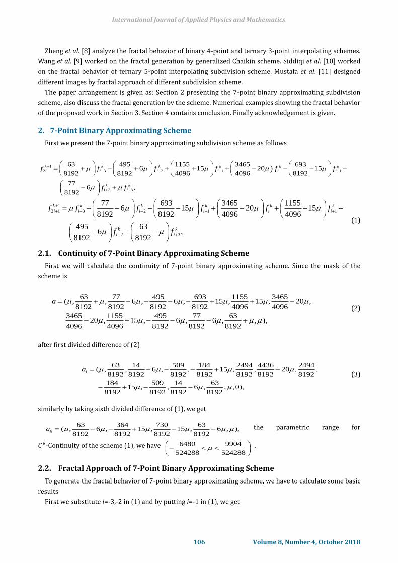
Fig. 2. (a) is the initial control pentagon where solid boxes show the initial control points. (b)-(d) show the

fourth, fifth and sixth refinement level at the parametric value 0.03 of 7-point binary approximating

scheme.

Fig. 1 (a) shows the initial rhombus and Fig. 1 (b)-(d) show the fractal generation at fourth, fifth and sixth

iteration. Similarly another initial closed polygon is shown in the Fig. 2 (a) and Fig. 2 (b)-(d) show the

fractal generation at fourth, fifth and sixth iteration. Fig. 1-2, we pick the value of parameter from the

fractal range discuss in the Cases 1-3 of 7-point binary approximating scheme.

4. Conclusion

We calculate the fractal properties of 7-point binary approximating subdivision scheme. Fractal approach

provide us the maximum deviation of limit curve instead of smoothness of the limit curve. As the scheme is

parametric, so by using different values of parameter we can generate different fractal curves according to

our own choice. In future, we will extend this work to regular and arbitrary topology.

Acknowledgement

This work is supported by NRPU Project No. 3183 and the SRGP Project No. 1741 of Higher Education

Commission (HEC) Pakistan.

References

[1] Rham, G., (1947). Un peude Mathematiques a proposed' une courbe plane. Revwe de Mathematiques

Elementry II, Oevred Completes, 2, 678-689.

[2] Dyn, N., Levin, D., & Gregory, J. A., (1987). A 4-point interpolatory subdivision scheme for curve design.

Computer Aided Geometric Design, 4(4), 257-268.

[3] Chaikin, G. M., (1974). An algorithm for high-speed curve generation. Computer Graphics and Image

Processing, 3(4), 346-349.

[4] Dubuc, S., (1986). Interpolation through an iterative scheme. Journal of Mathematical Analysis and

Applications, 114(1), 185-204.

[5] Boor, C., (1987). Cutting corners always works. Computer Aided Geometric Design, 4, 125-131.

[6] Weissman, A., (1990). A 6-Point Interpolatory Subdivision Scheme for Curve Design. M. Sc Thesis,

Tel-Aviv University, 189-199.

[7] Romani, L., (2009). From approximating subdivision schemes for exponential splines to

high-performance interpolating algorithms. Journal of Computational and Applied Mathematics, 224(1),

383-396.

[8] Zheng, H., Ye, Z., Lei, Y., & Liu, X., (2007). Fractal properties of interpolatory subdivision schemes and

their approximations in fractal generation. Chaos, Solitons and Fractals, 32, 113-123.

[9] Wang, J., Zheng, H., Xu, F., & Liu, D., (2011). Fractal properties of the generalized Chaikin corner-cutting

subdivision scheme. Computers and Mathematics with Applications, 61, 2197-2200.



[10] Siddiqi, S. S., Siddiqui, S., & Ahmad, N., (2014). Fractal generation using ternary 5-point interpolatory

subdivision scheme. Applied Mathematics and Computation, 234, 402-411.

[11] Mustafa, G., Bari, M., Jamil, S., (2016). Engineering images designed by fractal subdivision scheme.

SpringerPlus, 5(1), 1-10.

Mehwish Bari was born on 10th January, 1984, Bahawalpur, Pakistan. After getting the

basic education, she got the MSc (Mathematics) from The Islamia University of

Bahawalpur, Pakistan in 2005. She getting the Scholarship for M.Phil leading to the Ph.D.

in 2006 from Higher Education Commission Pakistan, complete M.Phil (mathematics) in

2009 and Ph.D. (mathematics) [computer aided geometric design] in 2016 from The

Islamia University of Bahawalpur, Pakistan.

Dr. Bari worked as research associate in the Department of Mathematics, the Islamia University of

Bahawalpur, Pakistan from 4th March, 2015 to 3rd March, 2018.

Dr. Bari worked as visiting lecturer, Department of Physics and Computer Science, the Islamia University

of Bahawalpur, Pakistan from February 2016 to June 2017.

Dr. Bari Currently working as chairperson, Department of Mathematics, National College of Business

Administration and Economics, Sub-Campus, Bahawalpur. Dr. Bari is a member of Organizing Committee,

International Pure Mathematics Conference.

Ghulam Mustafa was born on 5th January, 1973, Bahawalpur, Pakistan. After getting the

basic education, He got the MSc and M.Phil. (mathematics) degrees from Bahauddin

Zakariya University Multan, Pakistan in 1993 and 1996 respectively. He received a Ph.D.

(2004) in mathematics from the University of Science and Technology of China, P. R. China.

He did the post doctorate from Durham University UK sponsored by Association of

Commonwealth Universities UK 2011. He was visiting fellow at University of Science and

Technology of China from 2013-2014 sponsored by Chinese Academy of Sciences.

Currently, he is full professor of mathematics and chairman Department of Mathematics at The Islamia

University of Bahawalpur, Pakistan. His research interests include geometric modelling, applied

approximation theory.

Abid Hussain was born in 09/11/1985, Muzaffargarh, Pakistan. After getting the basic

education, he got the MSc mathematics degree in 2009 from the Islamia University of

Bahawalpur, Pakistan. He did M. Phil mathematics in 2016 from NCBA&E Sub-Campus

Bahawalpur, Pakistan.

Mr. Hussain is working as elementary school teacher, Punjnad colony school, district

Muzaffargarh, tehsil Alipur, Pakistan.

Author’s formal photo

fractal generation by 7-point binary approximating

Documents