fourierin: an r package to compute fourier integrals · fourierin: an r package to compute fourier...

CONTRIBUTED RESEARCH ARTICLE 72

fourierin: An R package to computeFourier integralsby Guillermo Basulto-Elias, Alicia Carriquiry, Kris De Brabanter and Daniel J. Nordman

Abstract We present the R package fourierin (Basulto-Elias, 2017) for evaluating functions defined asFourier-type integrals over a collection of argument values. The integrals are finitely supported withintegrands involving continuous functions of one or two variables. As an important application, suchFourier integrals arise in so-called “inversion formulas”, where one seeks to evaluate a probabilitydensity at a series of points from a given characteristic function (or vice versa) through Fouriertransforms. This paper intends to fill a gap in current R software, where tools for repeated evaluationof functions as Fourier integrals are not directly available. We implement two approaches for suchcomputations with numerical integration. In particular, if the argument collection for evaluationcorresponds to a regular grid, then an algorithm from Inverarity (2002) may be employed basedon a fast Fourier transform, which creates significant improvements in the speed over a secondapproach to numerical Fourier integration (where the latter also applies to cases where the points forevaluation are not on a grid). We illustrate the package with the computation of probability densitiesand characteristic functions through Fourier integrals/transforms, for both univariate and bivariateexamples.

Introduction

Continuous Fourier transforms commonly appear in several subject areas, such as physics and statis-tics. In probability theory, for example, continuous Fourier transforms are related to the characteristicfunction of a distribution and play an important role in evaluating probability densities from charac-teristic functions (and vice versa) through inversion formulas (cf. Athreya and Lahiri (2006)). SimilarFourier-type integrations are also commonly required in statistical methods for density estimation,such as kernel deconvolution (cf. Meister (2009)).

At issue, the Fourier integrals of interest often cannot be solved in elementary terms and typicallyrequire numerical approximations. As a compounding issue, the oscillating nature of the integrandsinvolved can cause numerical integration recipes to fail without careful consideration. However, Baileyand Swarztrauber (1994) present a mid-point integration rule in terms of appropriate discrete Fouriertransforms, which can be efficiently computed using the Fast Fourier Transform (FFT). Inverarity(2002) extended this characterization to the multivariate integral case. These works consequently offertargeted approaches for numerically approximating types of Fourier integrals of interest (e.g., in thecontext of characteristic or density functions).

Because R is one of the most popular programming languages among statisticians, it seemsworthwhile to have general tools available for computing such Fourier integrals in this softwareplatform. However, we have not found any R package that specifically performs this type of integralin general, though this integration does intrinsically occur in some statistical procedures. See ? foran application in kernel deconvolution where univariate Fourier integrals are required. Furthermore,beyond the integral form, the capacity to handle repeated calls for such integrals is another importantconsideration. This need arises when computing a function, that is itself defined by a Fourier integral,over a series of points. Note that this exact aspect occurs when determining a density function fromcharacteristic function (or vice versa), so that the ability to efficiently compute Fourier integrals over acollection of arguments is crucial.

The intent of the package fourierin explained here is to help in computing such Fourier-typeintegrals within R. The main function of the package serves to calculate Fourier integrals over a range ofpotential arguments for evaluation and is also easily adaptable to several definitions of the continuousFourier transform and its inverse (cf. Inverarity (2002)). (That is, the definition of a continuous Fouriertransform may change slightly from one context to another, often up to normalizing constants, sothat it becomes reasonable to provide a function that can accommodate any given definition throughscaling adjustments.) If the points for evaluating Fourier integrals are specified on regular grid, thenthe package allows use of the FFT for particularly fast numerical integration. However, the packagealso allow the user to evaluate such integrals at arbitrary collections of points that need not constitute aregular grid (though, in this case, the FFT cannot be used and computations naturally become slower).The latter can be handy in some situations; for example, evaluations at zero can provide momentsof a random variable when computing derivatives of a characteristic function from the probabilitydensity. The heavy computations in fourierin are performed in C++ via the RcppArmadillo package(cf. Eddelbuettel and Sanderson (2014)).

The R Journal Vol. 9/2, December 2017 ISSN 2073-4859

https://CRAN.R-project.org/package=fourierin

https://CRAN.R-project.org/package=RcppArmadillo


The rest of the paper has four sections. We first describe the Fourier integral for evaluation and itsnumerical approximation in “Fourier Integrals and Fast Fourier Transform (FFT).” We then illustratehow package fourierin may be used in univariate and bivariate cases of Fourier integration. In “SpeedComparison,” we demonstrate the two approaches (FFT-based or not) for computing Fourier integrals,both in one and two dimensions and at several grid sizes. We provide evidence that substantialtime savings occur when using the FFT-based method for evaluation at points on a grid. Finally, in“Summary,” we present conclusions and upcoming extensions to the R package.

Fourier integrals and fast Fourier transform

For w = (w1, . . . , wn), t = (t1, . . . , tn) ∈ Rn, define the vector dot product 〈w, t〉 = w1t1 + · · ·+ wntnand recall the complex exponential function exp{ıx} = cos(x) + ı sin(x), x ∈ R, where ı =

√−1.

This package aims to compute Fourier integrals at several points simultaneously, which namelyinvolves computation of the integral[

|s|(2π)1−r

]n/2 ∫ b1

a1

∫ b2

a2

· · ·∫ bn

an

f (t) exp {ıs〈w, t〉}dt, (1)

at more than one potential argument w ∈ Rn, where f is a generic continuous n-variate functionthat takes real or complex values, for n ∈ {1, 2}, and the above limits of integration are defined byreal values aj < bj for j = 1, . . . , n. Note that s and r in (1) denote real-valued constants, which areseparately included to permit some flexibility in the definition of continuous Fourier transforms tobe used (e.g., s = 1, r = 1). Hence, (1) represents a function of w ∈ Rn, defined by a Fourier integral,where the intention is to evaluate (1) over a discrete collection of w-values, often defined by a gridin Rn. For example, if [c1, d1)× · · · × [cn, dn) ⊂ Rn denotes a rectangular region specified by somereal constants cj < dj, j = 1, . . . , n, one may consider evaluating (1) at points w lying on a regular gridof size m1 ×m2 × · · · ×mn within [c1, d1)× · · · × [cn, dn), say, at points w(j1,...,jn) = (wj1 , . . . , wjn ) forwjk = ck + jk(dk − ck)/mk with jk ∈ {0, 1, . . . , mk − 1}, k = 1, . . . , n (where mk denotes the number ofgrid points in each coordinate dimension). Argument points on a grid are especially effective for fastapproximations of integrals (as in 1), as we discuss in the following.

At given argument w ∈ Rn, we numerically approximate the integral (1) with a discrete sumusing the mid-point rule, whereby the approximation of the j-th slice of the multiple integral involveslj partitioning rectangles (or equi-spaced subintervals) for j = 1, . . . , n and n ∈ {1, 2}; that is, forl1, . . . , ln representing a selection of the numbers of approximating nodes to be used in the coordinatesof integration (i.e., a resolution size), the integral (1) is approximated as n

∏j=1

bj − aj

lj

· [ |s|(2π)1−r

]n/2 l1−1

∑i1=0

l2−1

∑i2=0· · ·

ln−1

∑in=0

f (t(i1,...,in)) exp {ıs〈w, t(i1,...,in)〉}, (2)

with nodes t(i1,...,in) = (ti1 , . . . , tin ) defined by coordinate midpoints tik= ak +(2ik + 1)/2 · (bk− ak)/lk

for ik ∈ {0, 1, . . . , lk − 1} and k = 1, . . . , n. Note that a large grid size l1 × · · · × ln results in higherresolution for the integral approximation (2), but at a cost of increased computational effort. On theother hand, observe that when a regular grid is used, the upper evaluation limits, d1, . . . , dn are notincluded in such grid, however, the higher the resolution, the closer we get to these bounds.

To reiterate, the goal is then to evaluate the Fourier integral (1) over some set of argument pointsw ∈ Rn by employing the midpoint approximation (2), where the latter involves a l1 × · · · × lnresolution grid (of midpoint nodes) for n ∈ {1, 2}. It turns out that when the argument points w fallon a m1 × · · · ×mn-sized regular grid and this grid size matches the size of the approximating nodegrid from (2), namely lj = mj for each dimension j = 1, . . . , n, then the sum (2) may be written interms of certain discrete Fourier transforms and inverses of discrete Fourier transforms that can beconveniently computed with a FFT operation. Details of this derivation can be found in Inverarity(2002). It is well known that using FFT greatly reduces the computational complexity of discreteFourier transforms from O(m2) to O(m log m) in the univariate case, where m is the resolution or gridsize. The complexity of computing the multivariate discrete Fourier transform of an n-dimensionalarray using the FFT is O(M log M), where M = m1 · · ·mn and mj is the grid/resolution size in the j-thcoordinate direction, j = 1, . . . , n.

The R package fourierin can take advantage of such FFT representations for the fast computationof Fourier integrals evaluated on a regular grid. The package can also be used to evaluate Fourierintegrals at arbitrary discrete sets of points. The latter becomes important when one wishes to evaluatethe a continuous Fourier transform at only a few specific points (that may not necessarily constitute aregular grid). We later compare evaluation time of Fourier integrals on a regular grid, both using the



FFT and without using it in fourierin.

Examples

In this section we present examples to illustrate use of the fourierin package. We begin with aunivariate example which considers how to compute continuous Fourier transforms evaluated ona regular grid (therefore using the FFT operation) as well as how the computations proceed at threespecified points not on a regular grid (where the FFT is not be used). The second example considers atwo dimensional, or bivariate, case of Fourier integration.

The code that follows shows how the package can be used in univariate cases. The example weconsider is to recover a χ2 density f with five degrees of freedom from its characteristic function φ,where the underlying functions are given by

f (x) =1

25/2Γ(

52

) x52−1e−

x2 and φ(t) = (1− 2ıt)−5/2, (3)

for all x > 0 and t ∈ R. We also show how to use the package on non-regular grids. Specifically, wegenerate sample of three points from a χ2 distribution with five degrees of freedom and evaluate thedensity in Formula 3 at these three points where the density has been computed using the Fourierinversion formula approximated at four different resolutions. Results are presented in Table 1.

For illustration, the limits of integration are set from −10 to 10 and we compare several resolutions(64, 256 or 512) or grid node sizes for numerically performing integration (cf. (2)), recalling that thehigher the resolution, the better the integral approximation. To evaluate the integrals at argumentpoints on a regular grid, we choose [−3, 20] as an interval for specifying a collection of equi-spacedpoints, where the number of such points equals the resolution specified (as needed when using FFT).

## -------------------------------------------------------------------## Univariate example## -------------------------------------------------------------------

## Load packageslibrary(fourierin)library(dplyr)library(purrr)library(ggplot2)

## Set functionsdf <- 5cf <- function(t) (1 - 2i*t)^(-df/2)dens <- function(x) dchisq(x, df)

## Set resolutionsresolutions <- 2^(6:8)

## Compute integral given the resoltionrecover_f <- function(resol){

## Get grid and density valuesout <- fourierin(f = cf, lower_int = -10, upper_int = 10,

lower_eval = -3, upper_eval = 20,const_adj = -1, freq_adj = -1,resolution = resol)

## Return in dataframe formatout %>%

as_data_frame() %>%transmute(

x = w,values = Re(values),resolution = resol)

}

## Density approximationsvals <- map_df(resolutions, recover_f)



## True valuestrue <- data_frame(x = seq(min(vals$x), max(vals$x), length = 150),

values = dens(x))

univ_plot <-vals %>%mutate(resolution = as.character(resolution),

resolution = gsub("64", "064", resolution)) %>%ggplot(aes(x, values)) +geom_line(aes(color = resolution)) +geom_line(data = true, aes(color = "true values"))

univ_plot

## Evaluate in a nonregular gridset.seed(666)new_grid <- rchisq(n = 3, df = df)resolutions <- 2^(6:9)

fourierin(f = cf, lower_int = -10, upper_int = 10,eval_grid = new_grid,

const_adj = -1, freq_adj = -1,resolution = 128) %>%

c () %>% Re() %>%data_frame(x = new_grid, fx = .)

## Function that evaluates the log-density on new_grid at different## resolutions (i.e., number of points to approximate the integral in## the Fourier inversion formula).approximated_fx <- function (resol) {

fourierin(f = cf, lower_int = -10, upper_int = 12,eval_grid = new_grid,const_adj = -1, freq_adj = -1,resolution = resol) %>%

c() %>% Re() %>%{data_frame(x = new_grid,

fx = dens(new_grid),diffs = abs(. - fx),resolution = resol)}

}

## Generate tabletab <-

map_df(resolutions, approximated_fx) %>%arrange(x) %>%mutate(diffs = round(diffs, 7)) %>%rename('f(x)' = fx,

'absolute difference' = diffs)

tab

Observe that the first call of the fourierin function above has the default argument use_fft =TRUE. Therefore, this computation uses the the FFT representation described in Inverarity (2002) forregular grids, which is substantially fast (Figure 5, as described later, provides timing comparisonswithout the FFT for contrast). Also note that, when a regular evaluation grid is used, fourierin returnsa list with both the Fourier integral values and the evaluation grid. Figure 1 shows the resulting plotgenerated. A low resolution (64) for numerical integration has been included in order to observedifferences between the true density and its recovered version using Fourier integrals.

At the bottom of the code above, we also show how fourierin() works when a non-regular“evaluation grid” is provided. Observe that, in this case, one directly specifies separate points forevaluation of the integral in addition to separately specifying a resolution level for integration. Thisaspect is unlike the evaluation case on a regular grid. Consequently, only the Fourier integral values



x f (x) absolute difference resolution

3.0585883 0.1541368 0.0002072 640.0000476 1280.0000472 2560.0000471 512

6.4144242 0.0874281 0.0000780 640.0000155 1280.0000148 2560.0000147 512

11.7262677 0.0151776 0.0000097 640.0000025 1280.0000022 2560.0000022 512

Table 1: Absolute differences of true density values at three random points and density values at thesesame three points obtained using the Fourier inversion formula approximated at different resolutions.

0.00

0.05

0.10

0.15

0 5 10 15 20

x

valu

es

resolution

064

128

256

true values

Figure 1: Example of fourierin() function for univariate function at resolution 64. Recovering a χ2

density from its characteristic function. See Equation 3.

are returned, which is also unlike the regular grid case (where the evaluation grid is returned withcorresponding integrals in a list). Note that the function f from (1), when having a real-valuedargument, should be able to be evaluated at vectors in R.

In a second example, to illustrate how the fourierin() function works for bivariate functions, weuse a bivariate normal density f and find its characteristic function φ. In particular, we have theseunderlying functions as

f (x) =1√

2π|Σ|exp

[−1

2(x− µ)′Σ−1(x− µ)

]and φ(t) = exp

(ıx′µ− 1

2t′Σt

), (4)

for all t, x ∈ R2, with µ =

[−11

]and Σ =

[3 −1−1 3

].

Below is the code for this bivariate case using a regular evaluation grid, where the output is acomplex matrix whose components are Fourier integrals corresponding to the gridded set of bivariatearguments. As illustration, the limits of integration are set from (−8,−6) to (6, 8) (a square) and weconsider a resolution 128, where the range [−4, 4]× [−4, 4] is also chosen to define a collection ofevaluation points on a grid, where the number of such points again equals the resolution specified(i.e., for applying FFT).

## -------------------------------------------------------------------## Bivariate example## -------------------------------------------------------------------

## Load packages



library(fourierin)library(tidyr)library(dplyr)library(purrr)library(lattice)library(ggplot2)

## Set functions to be tested with their corresponding parameters.mu <- c(-1, 1)sig <- matrix(c(3, -1, -1, 2), 2, 2)

## Multivariate normal density, x is n x df <- function(x) {

## Auxiliar valuesd <- ncol(x)z <- sweep(x, 2, mu, "-")## Get numerator and denominator of normal densitynum <- exp(-0.5*rowSums(z * (z %*% solve(sig))))denom <- sqrt((2*pi)^d*det(sig))return(num/denom)

}

## Characteristic function, s is n x dphi <- function (s) {

complex(modulus = exp(-0.5*rowSums(s*(s %*% sig))),argument = s %*% mu)

}

## Evaluate characteristic function for a given resolution.eval <- fourierin(f,

lower_int = c(-8, -6), upper_int = c(6, 8),lower_eval = c(-4, -4), upper_eval = c(4, 4),const_adj = 1, freq_adj = 1,resolution = 2*c(64, 64),use_fft = T)

## Evaluate true and approximated values of Fourier integraldat <- eval %>%

with(crossing(y = w2, x = w1) %>%mutate(approximated = c(values))) %>%

mutate(true = phi(matrix(c(x, y), ncol = 2)),difference = approximated - true) %>%

gather(value, z, -x, -y) %>%mutate(real = Re(z), imaginary = Im(z)) %>%select(-z) %>%gather(part, z, -x, -y, -value)

## Surface plotwireframe(z ~ x*y | value*part, data = dat,

scales =list(arrows=FALSE, cex= 0.45,

col = "black", font = 3, tck = 1),screen = list(z = 90, x = -74),colorkey = FALSE,shade=TRUE,light.source= c(0,10,10),shade.colors = function(irr, ref,

height, w = 0.4)grey(w*irr + (1 - w)*(1 - (1 - ref)^0.4)),

aspect = c(1, 0.65))

## Contours of valuesbiv_example1 <-



dat %>%filter(value != "difference") %>%ggplot(aes(x, y, z = z)) +geom_tile(aes(fill = z)) +facet_grid(part ~ value) +scale_fill_distiller(palette = "Reds")

biv_example1

## Contour of differencesbiv_example2 <-

dat %>%filter(value == "difference") %>%ggplot(aes(x, y, z = z)) +geom_tile(aes(fill = z)) +facet_grid(part ~ value) +scale_fill_distiller(palette = "Spectral")

biv_example2

The result of fourierin() was stored above in eval, which is a list with three elements: twovectors with the corresponding evaluation grid values in each coordinate direction and a complexmatrix containing the Fourier integral values. If we do not wish to evaluate the Fourier integrals on aregular grid and instead wish to evaluate these at, say l bivariate points, then we must pass a l × 2matrix in the argument w and the function will return a vector of size l with the Fourier integrals,rather than a list. In the bivariate situation here, the function f must be able to receive a two-columnmatrix with m rows, where m is the number of points where the Fourier integral will be evaluated.

Corresponding to this bivariate example, we have generated three plots to compare the approx-imation from Fourier integrals to the underlying truth (i.e., compare the approximated and truecharacteristic functions of the bivariate normal distribution). In Figure 2, we present the surface plotsof the approximated and the true values, as well as their differences for both the real and imaginaryparts. One observes that differences are small, indicating the adequacy of the numerical integration.

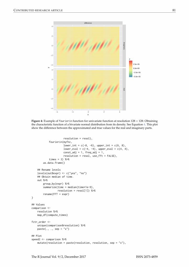
For a different perspective of the resulting Fourier integration, Figure 3 presents a contour plotshowing the approximated and true values of the bivariate normal characteristic function, for bothreal and imaginary parts. We show a tile plot of the differences in Figure 4. Observe that the range ofdifferences in Figure 4 is relatively much smaller than the values in Figure 3.

Speed comparison

Through a small numerical study, here we compare the differences in execution times using fourierin()for integration at points on a regular grid, both with or without FFT steps, considering univariateand bivariate Fourier integrals. Figure 5 shows timing results for a univariate example of the integralin (1) evaluated on a grid, while Figure 6 presents timing results for a bivariate example. Note thatthe reported time units differ between these figures, as the bivariate case naturally requires moretime. These figures provide evidence that, for evaluating integrals on a regular grid, the FFT option infourierin() creates large advantages in time.

The code that was used to generate Figure 5 and 6 is below.

## -------------------------------------------------------------------## Univariate speed test## -------------------------------------------------------------------

library(fourierin)library(dplyr)library(purrr)library(ggplot2)library(microbenchmark)

## Test speed at several resolutionsresolution <- 2^(3:8)

## Function to be tested



−4

−2

0

2

−4−202

0.0

0.5

1.0

x

y

z

approximatedimaginary

−4

−2

0

2

−4−202

0.0

0.5

1.0

x

y

z

differenceimaginary

−4

−2

0

2

−4−202

0.0

0.5

1.0

x

y

z

trueimaginary

−4

−2

0

2

−4−202

0.0

0.5

1.0

x

y

z

approximatedreal

−4

−2

0

2

−4−202

0.0

0.5

1.0

x

y

z

differencereal

−4

−2

0

2

−4−202

0.0

0.5

1.0

x

y

z

truereal

Figure 2: Example of fourierin function for univariate function at resolution 128× 128: Obtainingthe characteristic function of a bivariate normal distribution from its density. See Equation 4. Thispanel contains every combination of approximation-true-difference with real-imaginary parts.

myfnc <- function(t) exp(-t^2/2)

## Aux. functioncompute_times <- function(resol){

out <-microbenchmark(

fourierin_1d(f = myfnc, -5, 5, -3, 3, -1, -1, resol),fourierin_1d(f = myfnc, -5, 5, -3, 3, -1, -1, resol,

use_fft = FALSE),times = 5) %>%

as.data.frame()## Rename levelslevels(out$expr) <- c("yes", "no")## Obtain median of time.out %>%

group_by(expr) %>%summarize(time = median(time*1e-6),

resolution = resol) %>%rename(FFT = expr)

}

speed1 <- resolution %>%map_df(compute_times) %>%mutate(resolution = as.factor(resolution)) %>%ggplot(aes(resolution, log(time), color = FFT)) +geom_point(size = 2, aes(shape = FFT)) +



approximated true

imaginary

real

−4 −2 0 2 4 −4 −2 0 2 4

−4

−2

0

2

4

−4

−2

0

2

4

x

y

0.0

0.5

1.0z

Figure 3: Example of fourierin function for univariate function at resolution 128× 128: Obtainingthe characteristic function of a bivariate normal distribution from its density. See Equation 4. Eachcombination the approximated and true values are shown for both the real and imaginary parts.

geom_line(aes(linetype = FFT, group = FFT)) +ylab("time (in log-milliseconds)")

speed1

## -------------------------------------------------------------------## Bivariate test## -------------------------------------------------------------------

## Load packageslibrary(fourierin)library(dplyr)library(purrr)library(ggplot2)library(microbenchmark)

## Test speed at several resolutionsresolution <- 2^(3:7)

## Bivariate function to be testedmyfnc <- function(x) dnorm(x[, 1])*dnorm(x[, 2])

## Aux. functioncompute_times <- function(resol){

resol <- rep(resol, 2)out <-

microbenchmark(fourierin(myfnc,

lower_int = c(-8, -6), upper_int = c(6, 8),lower_eval = c(-4, -4), upper_eval = c(4, 4),const_adj = 1, freq_adj = 1,



difference

imaginary

real

−4 −2 0 2 4

−4

−2

0

2

4

−4

−2

0

2

4

x

y

−5.0e−05

−2.5e−05

0.0e+00

2.5e−05

z

Figure 4: Example of fourierin function for univariate function at resolution 128× 128: Obtainingthe characteristic function of a bivariate normal distribution from its density. See Equation 4. This plotshow the difference between the approximated and true values for the real and imaginary parts.

resolution = resol),fourierin(myfnc,

lower_int = c(-8, -6), upper_int = c(6, 8),lower_eval = c(-4, -4), upper_eval = c(4, 4),const_adj = 1, freq_adj = 1,resolution = resol, use_fft = FALSE),

times = 3) %>%as.data.frame()

## Rename levelslevels(out$expr) <- c("yes", "no")## Obtain median of time.out %>%

group_by(expr) %>%summarize(time = median(time*1e-9),

resolution = resol[1]) %>%rename(FFT = expr)

}

## Valuescomparison <-

resolution %>%map_df(compute_times)

fctr_order <-unique(comparison$resolution) %>%paste(., ., sep = "x")

## Plotspeed2 <- comparison %>%

mutate(resolution = paste(resolution, resolution, sep = "x"),



●

●

●

●

●

●

−3

−2

−1

0

1

8 16 32 64 128 256

resolution

time

(in lo

g−m

illis

econ

ds)

FFT● yes

no

Figure 5: Example of a univariate Fourier integral over grids of several (power of two) sizes. Specifi-cally, the standard normal density is being recovered using the Fourier inversion formula. Time is inlog-milliseconds. The Fourier integral has been applied five times for every resolution and each dotrepresents the mean for the corresponding grid size and method. Observe that both, x and y axis arein logarithmic scale.

resolution = ordered(resolution, levels = fctr_order)) %>%ggplot(aes(resolution, log(time), color = FFT)) +geom_point(size = 2, aes(shape = FFT)) +geom_line(aes(linetype = FFT, group = FFT)) +ylab("time (in log-seconds)")

speed2

Summary

Continuous Fourier integrals/transforms are useful in statistics for computation of probability densi-ties from characteristic functions, as well as the reverse, when describing probability structure; seethe “Examples” section for some demonstrations. The usefulness and potential application of Fourierintegrals, however, also extends to other contexts of physics and mathematics, as well as to statisticalinference (e.g., types of density estimation). For this reason, we have developed the fourierin packageas a tool for computing Fourier integrals over collections of evaluation points, where repeat evaluationsteps and often complicated numerical integrations are involved. When evaluation points fall on aregular grid, fourierin allows use of a Fast Fourier Transform as a key ingredient for rapid numericalapproximation of Fourier-type integrals.

In “Speed Comparison,” we presented evidence of the gain in time when using this fast imple-mentation of fourierin() on regular grids, while we also illustrated the versatility of fourierin in“Examples” section. At present (version 0.2.1), the fourierin package performs univariate and bivariateFourier integration. An extension of the package to address higher dimensional integration will beincluded in future versions.

Bibliography

K. B. Athreya and S. N. Lahiri. Measure theory and probability theory. Springer Science & Business Media,2006. [p72]

D. H. Bailey and P. N. Swarztrauber. A fast method for the numerical evaluation of continuous Fourierand Laplace transforms. SIAM Journal on Scientific Computing, 15(5):1105–1110, 1994. [p72]

G. Basulto-Elias. fourierin: Computes Numeric Fourier Integrals, 2017. URL https://CRAN.R-project.org/package=fourierin. R package version 0.2.2. [p72]

D. Eddelbuettel and C. Sanderson. Rcpparmadillo: Accelerating R with high-performance C++linear algebra. Computational Statistics and Data Analysis, 71:1054–1063, March 2014. URL http://dx.doi.org/10.1016/j.csda.2013.02.005. [p72]




http://dx.doi.org/10.1016/j.csda.2013.02.005

http://dx.doi.org/10.1016/j.csda.2013.02.005


●

●

●

●

●

−6

−3

0

8x8 16x16 32x32 64x64 128x128

resolution

time

(in lo

g−se

cond

s)

FFT● yes

no

Figure 6: Example of a bivariate Fourier integral over grids of several (power of two) sizes. Both axishave the same resolution. Specifically, the characteristic function of a bivariate normal distribution isbeing computed. Time is in log-seconds (unlike 5). The Fourier integral has been applied five timesfor every resolution and each dot represents the mean for the corresponding grid size and method.Observe that both, x and y axis are in logarithmic scale.

G. Inverarity. Fast computation of multidimensional Fourier integrals. SIAM Journal on ScientificComputing, 24(2):645–651, 2002. [p72, 73, 75]

A. Meister. Deconvolution problems in nonparametric statistics, volume 193. Springer, 2009. [p72]

Guillermo Basulto-EliasIowa State UniversityAmes, IAUnited [email protected]

Alicia CarriquiryIowa State UniversityAmes, IAUnited [email protected]

Kris De BrabanterIowa State UniversityAmes, IAUnited [email protected]

Daniel J. NordmanIowa State UniversityAmes, IAUnited [email protected]


mailto:[email protected]




fourierin: an r package to compute fourier integrals · fourierin: an r package to compute fourier...

Documents