fourier transform with rotations on circles and ellipses
TRANSCRIPT
Fourier Transform with
Rotations on Circles
and Ellipses
in Signal and Image ProcessingArtyom M. Grigoryan
Department of Electrical and Computer EngineeringUniversity of Texas at San Antonio One UTSA Circle,
San Antonio, USA TX 78249e-mail: [email protected]
Introduction
We analyze the general concept of rotation and pro-cessing of data around not only circles but ellipses, ingeneral. The general concept of the elliptic Fouriertransform which was developed by [Grigoryan, 2009].The block-wise representation of the discrete Fouriertransform (DFT) is considered in the real space, whichis effective and that can be generalized to obtain newmethods in spectral analysis. The N-point Elliptic DFT(EDFT) uses as a basic 2 × 2 transformation the rota-tions around ellipses.
The EDFT distinguishes well from the carrying frequen-cies of the signal in both real and imaginary parts. Italso has a simple inverse matrix. It is parameterizedand includes also the DFT. Our preliminary results showthat by using different parameters, the EDFT can beused effectively for solving many problems in signal andimage processing field, in which includes problems suchas image enhancement, filtration, encryption and manyothers.
1
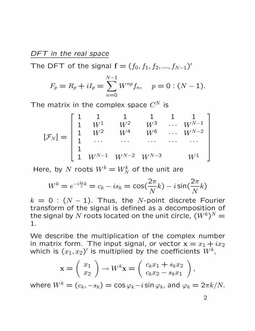
DFT in the real space
The DFT of the signal f = (f0, f1, f2, ..., fN−1)′
Fp = Rp + iIp =
N−1∑
n=0
W npfn, p = 0 : (N − 1).
The matrix in the complex space CN is
[FN ] =
1 1 1 1 1 11 W 1 W 2 W 3 · · · W N−1
1 W 2 W 4 W 6 · · · W N−2
1 · · · · · · · · · · · · · · ·11 W N−1 W N−2 W N−3 W 1
Here, by N roots W k = W kN of the unit are
W k = e−i2π
Nk = ck − isk = cos(
2π
Nk)− i sin(
2π
Nk)
k = 0 : (N − 1). Thus, the N-point discrete Fouriertransform of the signal is defined as a decomposition ofthe signal by N roots located on the unit circle, (W k)N =1.
We describe the multiplication of the complex numberin matrix form. The input signal, or vector x = x1 + ix2
which is (x1, x2)′ is multiplied by the coefficients W k,
x =
(
x1
x2
)
→ W kx =
(
ckx1 + skx2
ckx2 − skx1
)
,
where W k = (ck,−sk) = cosϕk−i sinϕk, and ϕk = 2πk/N.
2
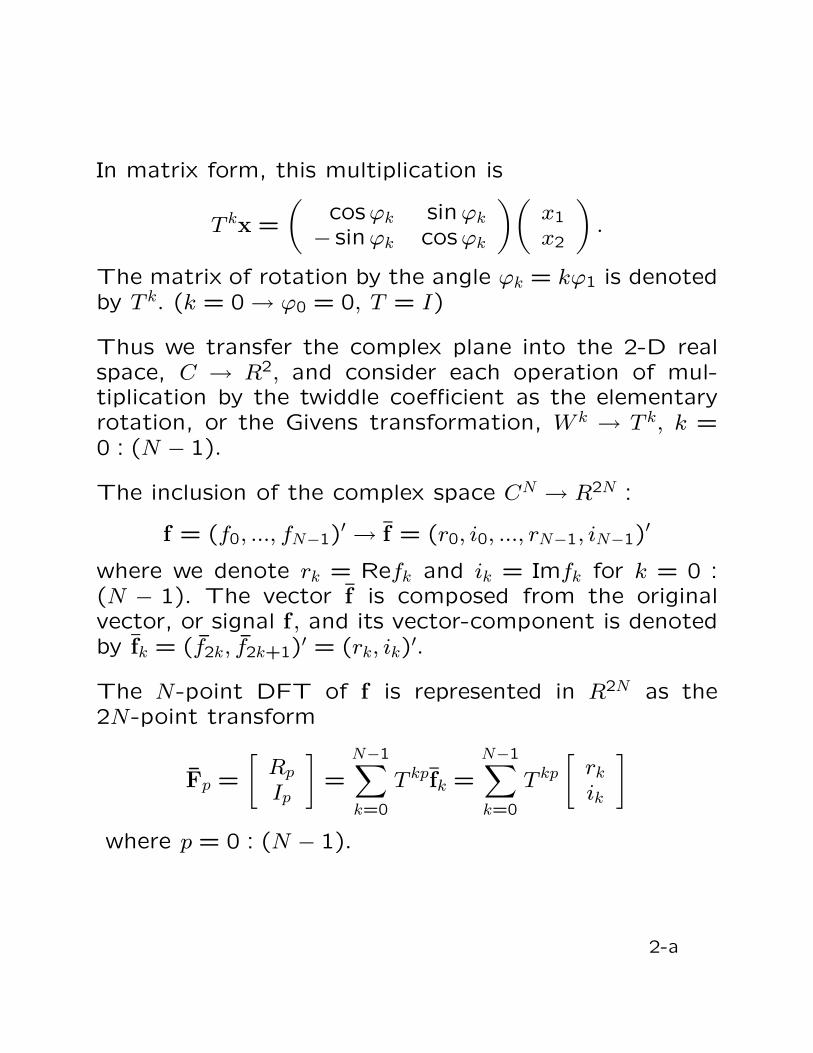
In matrix form, this multiplication is
T kx =
(
cosϕk sinϕk
− sinϕk cosϕk
)(
x1
x2
)
.
The matrix of rotation by the angle ϕk = kϕ1 is denotedby T k. (k = 0 → ϕ0 = 0, T = I)
Thus we transfer the complex plane into the 2-D realspace, C → R2, and consider each operation of mul-tiplication by the twiddle coefficient as the elementaryrotation, or the Givens transformation, W k → T k, k =0 : (N − 1).
The inclusion of the complex space CN → R2N :
f = (f0, ..., fN−1)′ → f̄ = (r0, i0, ..., rN−1, iN−1)
′
where we denote rk = Refk and ik = Imfk for k = 0 :(N − 1). The vector f̄ is composed from the originalvector, or signal f , and its vector-component is denotedby f̄k = (f̄2k, f̄2k+1)
′ = (rk, ik)′.
The N-point DFT of f is represented in R2N as the2N-point transform
F̄p =
[
Rp
Ip
]
=
N−1∑
k=0
T kpf̄k =
N−1∑
k=0
T kp
[
rk
ik
]
where p = 0 : (N − 1).
2-a
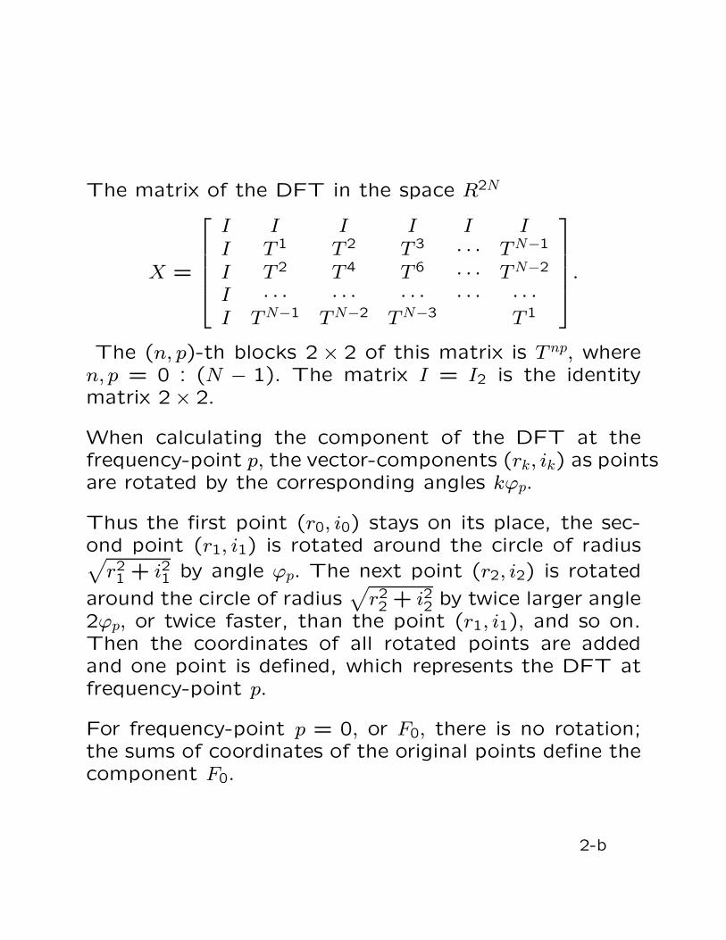
The matrix of the DFT in the space R2N
X =
I I I I I II T 1 T 2 T 3 · · · T N−1
I T 2 T 4 T 6 · · · T N−2
I · · · · · · · · · · · · · · ·I T N−1 T N−2 T N−3 T 1
.
The (n, p)-th blocks 2 × 2 of this matrix is T np, wheren, p = 0 : (N − 1). The matrix I = I2 is the identitymatrix 2 × 2.
When calculating the component of the DFT at thefrequency-point p, the vector-components (rk, ik) as pointsare rotated by the corresponding angles kϕp.
Thus the first point (r0, i0) stays on its place, the sec-ond point (r1, i1) is rotated around the circle of radius√
r21 + i21 by angle ϕp. The next point (r2, i2) is rotated
around the circle of radius√
r22 + i22 by twice larger angle
2ϕp, or twice faster, than the point (r1, i1), and so on.Then the coordinates of all rotated points are addedand one point is defined, which represents the DFT atfrequency-point p.
For frequency-point p = 0, or F0, there is no rotation;the sums of coordinates of the original points define thecomponent F0.
2-b
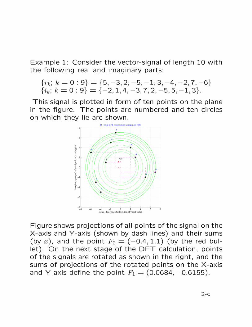
Example 1: Consider the vector-signal of length 10 withthe following real and imaginary parts:
{rk; k = 0 : 9} = {5,−3,2,−5,−1,3,−4,−2,7,−6}{ik; k = 0 : 9} = {−2,1,4,−3,7,2,−5,5,−1,3}.
This signal is plotted in form of ten points on the planein the figure. The points are numbered and ten circleson which they lie are shown.
−8 −6 −4 −2 0 2 4 6 8−8
−6
−4
−2
0
2
4
6
8
10−point DFT composition: component F(0).
signal−data (black bullets), the DFT (red bullet)
imag
inar
y p
art
y(n
) o
f th
e si
gn
al z
(n)=
x(n
)+jy
(n)
0
1
2
3
4
5
6
7
8
9
F(0)
Figure shows projections of all points of the signal on theX-axis and Y-axis (shown by dash lines) and their sums(by x), and the point F0 = (−0.4, 1.1) (by the red bul-let). On the next stage of the DFT calculation, pointsof the signals are rotated as shown in the right, and thesums of projections of the rotated points on the X-axisand Y-axis define the point F1 = (0.0684,−0.6155).
2-c
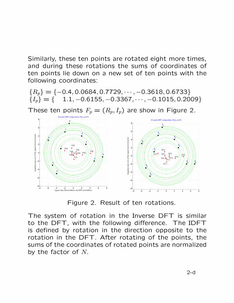
Similarly, these ten points are rotated eight more times,and during these rotations the sums of coordinates often points lie down on a new set of ten points with thefollowing coordinates:
{Rp} = {−0.4,0.0684,0.7729, · · · ,−0.3618,0.6733}{Ip} = { 1.1,−0.6155,−0.3367, · · · ,−0.1015,0.2009}
These ten points Fp = (Rp, Ip) are show in Figure 2.
−8 −6 −4 −2 0 2 4 6 8−8
−6
−4
−2
0
2
4
6
8
10−point DFT composition: F(p), p=0:9.
signal−data (black bullets), the DFT (red bullets)
imag
inar
y p
art
y(n
) of
the
signal
z(n
)=x(n
)+jy
(n)
0
1
2
3
4
5
6
7
8
9
F(0)
F(1) F(2)
F(3)
F(4)F(5)
F(6)
F(7)
F(8)F(9)
−8 −6 −4 −2 0 2 4 6 8
−8
−6
−4
−2
0
2
4
6
8
10−point DFT composition: F(p), p=0:9.
imag
inar
y p
art
y(n
) of
the
signal
z(n
)=x(n
)+jy
(n)
f0
f1
f2
f3
f4
f5
f6
f7
f8
f9
F(0)
F(1)F(2)
F(3) F(4)F(5)
F(6)
F(7)
F(8) F(9)
f0
f1
f2
f3
f4
f5
f6
f7
f8
f9
Figure 2. Result of ten rotations.
The system of rotation in the Inverse DFT is similarto the DFT, with the following difference. The IDFTis defined by rotation in the direction opposite to therotation in the DFT. After rotating of the points, thesums of the coordinates of rotated points are normalizedby the factor of N.
2-d

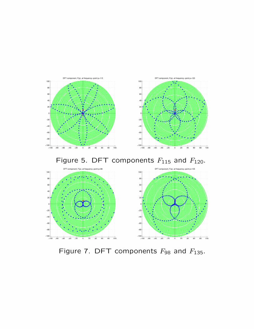
DFT and Horoscope
Consider the following symmetric complex signal fn :
fn = rn + jin = n + j(n/5), f−n = fn, n = 0 : 200.
Next figures illustrate the geometry of a few compo-nents Fp of the 201-point DFT.
−100 −80 −60 −40 −20 0 20 40 60 80 100
−100
−80
−60
−40
−20
0
20
40
60
80
100
DFT component, F(p), at frequency−point p=1
0
−100 −80 −60 −40 −20 0 20 40 60 80 100
−100
−80
−60
−40
−20
0
20
40
60
80
100
DFT component, F(p), at frequency−point p=2
0
Figure 3. DFT components F1 and F2.
−100 −80 −60 −40 −20 0 20 40 60 80 100
−100
−80
−60
−40
−20
0
20
40
60
80
100
DFT component, F(p), at frequency−point p=3
0
−100 −80 −60 −40 −20 0 20 40 60 80 100
−100
−80
−60
−40
−20
0
20
40
60
80
100
DFT component, F(p), at frequency−point p=4
0
Figure 4. DFT components F3 and F4.
3
−100 −80 −60 −40 −20 0 20 40 60 80 100
−100
−80
−60
−40
−20
0
20
40
60
80
100
DFT component, F(p), at frequency−point p=115
0
−100 −80 −60 −40 −20 0 20 40 60 80 100
−100
−80
−60
−40
−20
0
20
40
60
80
100
DFT component, F(p), at frequency−point p=120
0
Figure 5. DFT components F115 and F120.
−100 −80 −60 −40 −20 0 20 40 60 80 100
−100
−80
−60
−40
−20
0
20
40
60
80
100
DFT component, F(p), at frequency−point p=98
0
−100 −80 −60 −40 −20 0 20 40 60 80 100
−100
−80
−60
−40
−20
0
20
40
60
80
100
DFT component, F(p), at frequency−point p=135
0
Figure 7. DFT components F98 and F135.
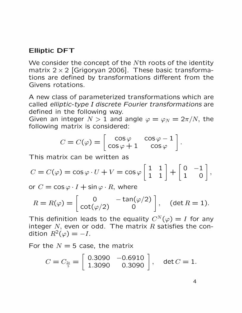
Elliptic DFT
We consider the concept of the Nth roots of the identitymatrix 2× 2 [Grigoryan 2006]. These basic transforma-tions are defined by transformations different from theGivens rotations.
A new class of parameterized transformations which arecalled elliptic-type I discrete Fourier transformations aredefined in the following way.Given an integer N > 1 and angle ϕ = ϕN = 2π/N, thefollowing matrix is considered:
C = C(ϕ) =
[
cos ϕ cosϕ − 1cosϕ + 1 cos ϕ
]
.
This matrix can be written as
C = C(ϕ) = cos ϕ · U + V = cosϕ
[
1 11 1
]
+
[
0 −11 0
]
,
or C = cos ϕ · I + sinϕ · R, where
R = R(ϕ) =
[
0 − tan(ϕ/2)cot(ϕ/2) 0
]
, (det R = 1).
This definition leads to the equality CN(ϕ) = I for anyinteger N, even or odd. The matrix R satisfies the con-dition R2(ϕ) = −I.
For the N = 5 case, the matrix
C = C2π
5=
[
0.3090 −0.69101.3090 0.3090
]
, det C = 1.
4
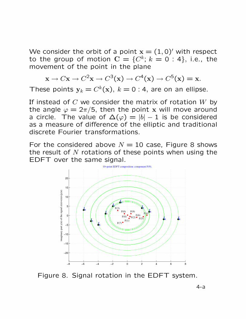
We consider the orbit of a point x = (1,0)′ with respectto the group of motion C = {Ck; k = 0 : 4}, i.e., themovement of the point in the plane
x → Cx → C2x → C3(x) → C4(x) → C5(x) = x.
These points yk = Ck(x), k = 0 : 4, are on an ellipse.
If instead of C we consider the matrix of rotation W bythe angle ϕ = 2π/5, then the point x will move arounda circle. The value of ∆(ϕ) = |b| − 1 is be consideredas a measure of difference of the elliptic and traditionaldiscrete Fourier transformations.
For the considered above N = 10 case, Figure 8 showsthe result of N rotations of these points when using theEDFT over the same signal.
−8 −6 −4 −2 0 2 4 6 8
−20
−15
−10
−5
0
5
10
15
20
10−point EDFT composition: component F(9).
imag
inar
y p
art
y(n
) o
f th
e si
gnal
z(n
)=x(n
)+jy
(n)
f0
f1
f2
f3
f4
f5
f6
f7
f8
f9
F(0)
F(1)
F(2)
F(3)
F(4)
F(5)
F(6)
F(7)
F(8)
F(9)
f0
f1
f2
f3
f4
f5
f6
f7
f8
f9
Figure 8. Signal rotation in the EDFT system.
4-a
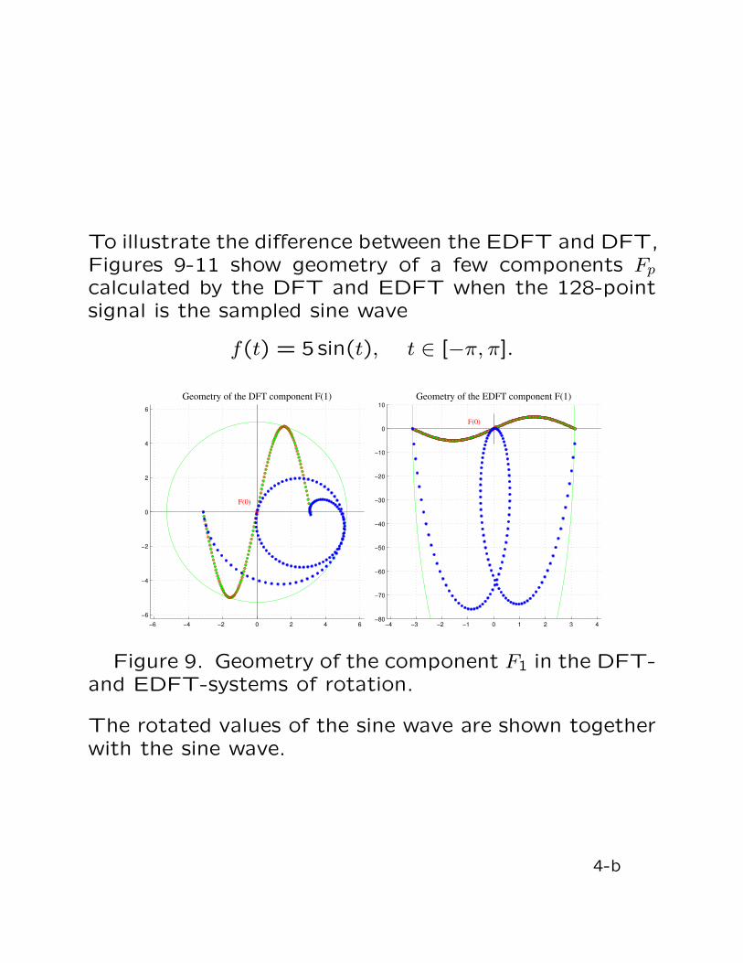
To illustrate the difference between the EDFT and DFT,Figures 9-11 show geometry of a few components Fp
calculated by the DFT and EDFT when the 128-pointsignal is the sampled sine wave
f(t) = 5 sin(t), t ∈ [−π, π].
−6 −4 −2 0 2 4 6
−6
−4
−2
0
2
4
6
Geometry of the DFT component F(1)
F(0)
−4 −3 −2 −1 0 1 2 3 4−80
−70
−60
−50
−40
−30
−20
−10
0
10
Geometry of the EDFT component F(1)
0F(0)
Figure 9. Geometry of the component F1 in the DFT-and EDFT-systems of rotation.
The rotated values of the sine wave are shown togetherwith the sine wave.
4-b
−6 −4 −2 0 2 4 6
−6
−4
−2
0
2
4
6
Geometry of the DFT component F(2)
F(0)
−4 −3 −2 −1 0 1 2 3 4−100
−50
0
50
Geometry of the EDFT component F(2)
0F(0)
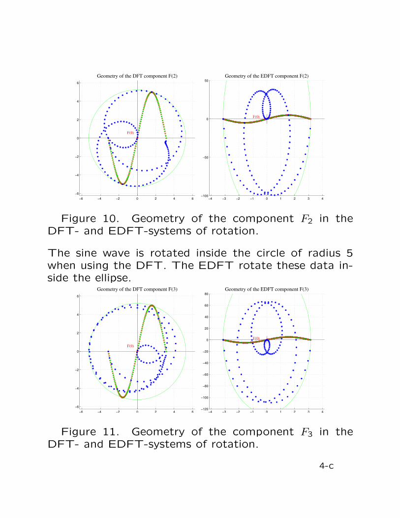
Figure 10. Geometry of the component F2 in theDFT- and EDFT-systems of rotation.
The sine wave is rotated inside the circle of radius 5when using the DFT. The EDFT rotate these data in-side the ellipse.
−6 −4 −2 0 2 4 6
−6
−4
−2
0
2
4
6
Geometry of the DFT component F(3)
F(0)
−4 −3 −2 −1 0 1 2 3 4−120
−100
−80
−60
−40
−20
0
20
40
60
80
Geometry of the EDFT component F(3)
0F(0)
Figure 11. Geometry of the component F3 in theDFT- and EDFT-systems of rotation.
4-c
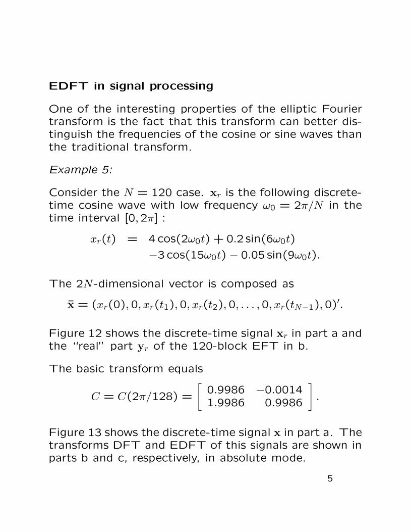
EDFT in signal processing
One of the interesting properties of the elliptic Fouriertransform is the fact that this transform can better dis-tinguish the frequencies of the cosine or sine waves thanthe traditional transform.
Example 5:
Consider the N = 120 case. xr is the following discrete-time cosine wave with low frequency ω0 = 2π/N in thetime interval [0,2π] :
xr(t) = 4cos(2ω0t) + 0.2 sin(6ω0t)
−3cos(15ω0t) − 0.05 sin(9ω0t).
The 2N-dimensional vector is composed as
x̄ = (xr(0), 0, xr(t1),0, xr(t2),0, . . . ,0, xr(tN−1),0)′.
Figure 12 shows the discrete-time signal xr in part a andthe “real” part yr of the 120-block EFT in b.
The basic transform equals
C = C(2π/128) =
[
0.9986 −0.00141.9986 0.9986
]
.
Figure 13 shows the discrete-time signal x in part a. Thetransforms DFT and EDFT of this signals are shown inparts b and c, respectively, in absolute mode.
5
0 1 2 3 4 5 6−10
−5
0
5
10
(a)
x(n)
0 1 2 3 4 5 60
100
200
300
400
500
(b)|EDFT|
0 1 2 3 4 5 60
100
200
300
(c)
|DFT|
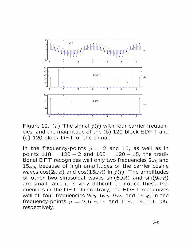
Figure 12. (a) The signal f(t) with four carrier frequen-cies, and the magnitude of the (b) 120-block EDFT and(c) 120-block DFT of the signal.
In the frequency-points p = 2 and 15, as well as inpoints 118 = 120 − 2 and 105 = 120 − 15, the tradi-tional DFT recognizes well only two frequencies 2ω0 and15ω0, because of high amplitudes of the carrier cosinewaves cos(2ω0t) and cos(15ω0t) in f(t). The amplitudesof other two sinusoidal waves sin(6ω0t) and sin(9ω0t)are small, and it is very difficult to notice these fre-quencies in the DFT. In contrary, the EDFT recognizeswell all four frequencies 2ω0, 6ω0, 9ω0, and 15ω0, in thefrequency-points p = 2,6,9,15 and 118,114,111,105,respectively.
5-a
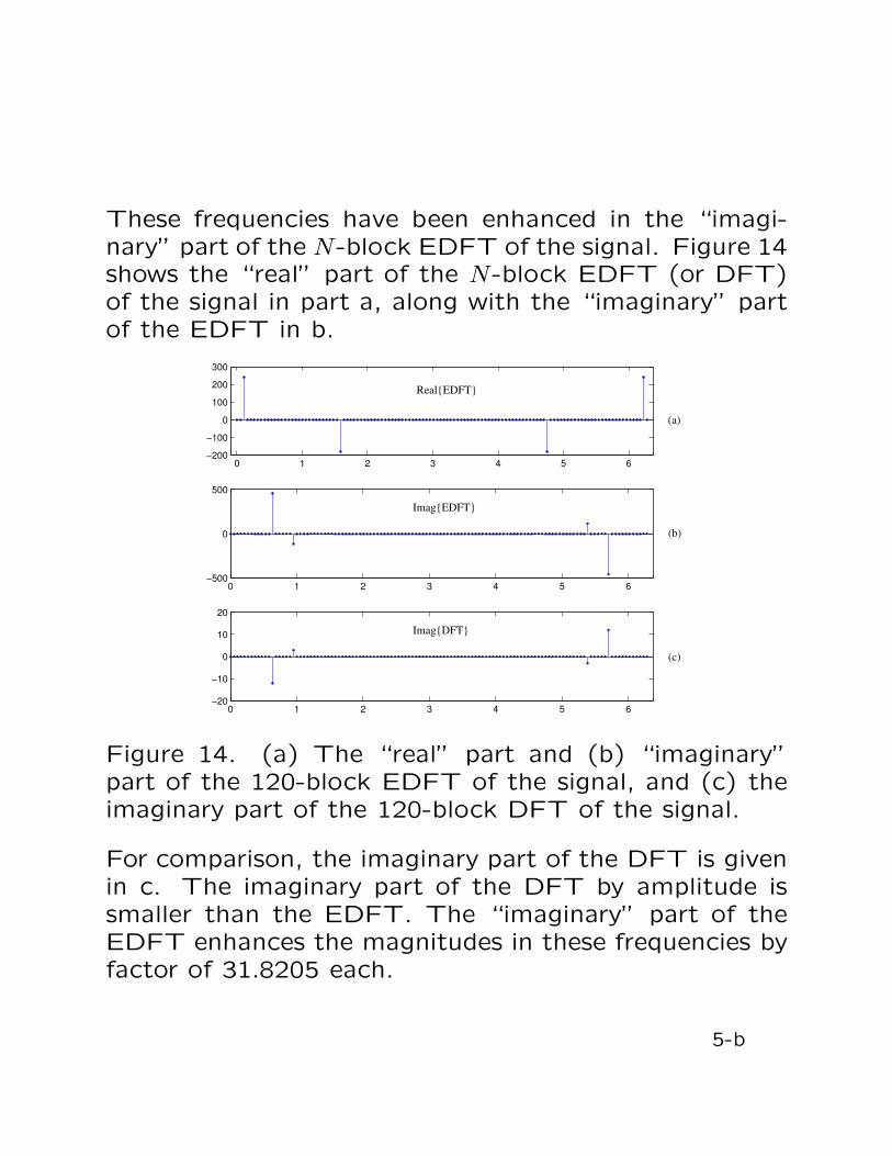
These frequencies have been enhanced in the “imagi-nary” part of the N-block EDFT of the signal. Figure 14shows the “real” part of the N-block EDFT (or DFT)of the signal in part a, along with the “imaginary” partof the EDFT in b.
0 1 2 3 4 5 6−200
−100
0
100
200
300
(a)
Real{EDFT}
0 1 2 3 4 5 6−500
0
500
(b)
Imag{EDFT}
0 1 2 3 4 5 6−20
−10
0
10
20
(c)
Imag{DFT}
Figure 14. (a) The “real” part and (b) “imaginary”part of the 120-block EDFT of the signal, and (c) theimaginary part of the 120-block DFT of the signal.
For comparison, the imaginary part of the DFT is givenin c. The imaginary part of the DFT by amplitude issmaller than the EDFT. The “imaginary” part of theEDFT enhances the magnitudes in these frequencies byfactor of 31.8205 each.
5-b
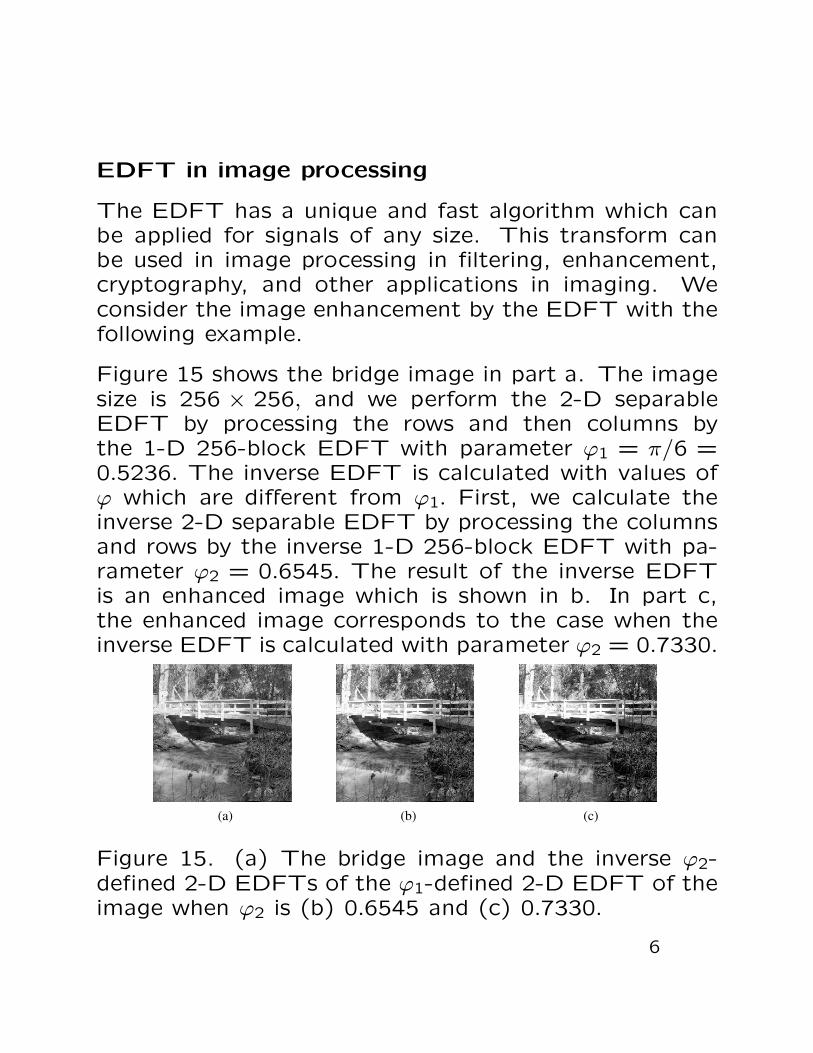
EDFT in image processing
The EDFT has a unique and fast algorithm which canbe applied for signals of any size. This transform canbe used in image processing in filtering, enhancement,cryptography, and other applications in imaging. Weconsider the image enhancement by the EDFT with thefollowing example.
Figure 15 shows the bridge image in part a. The imagesize is 256 × 256, and we perform the 2-D separableEDFT by processing the rows and then columns bythe 1-D 256-block EDFT with parameter ϕ1 = π/6 =0.5236. The inverse EDFT is calculated with values ofϕ which are different from ϕ1. First, we calculate theinverse 2-D separable EDFT by processing the columnsand rows by the inverse 1-D 256-block EDFT with pa-rameter ϕ2 = 0.6545. The result of the inverse EDFTis an enhanced image which is shown in b. In part c,the enhanced image corresponds to the case when theinverse EDFT is calculated with parameter ϕ2 = 0.7330.
(a) (b) (c)
Figure 15. (a) The bridge image and the inverse ϕ2-defined 2-D EDFTs of the ϕ1-defined 2-D EDFT of theimage when ϕ2 is (b) 0.6545 and (c) 0.7330.
6
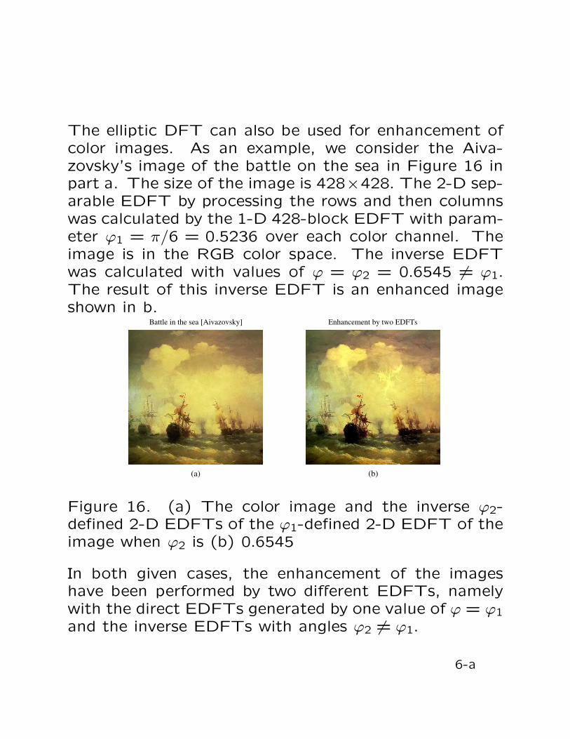
The elliptic DFT can also be used for enhancement ofcolor images. As an example, we consider the Aiva-zovsky’s image of the battle on the sea in Figure 16 inpart a. The size of the image is 428×428. The 2-D sep-arable EDFT by processing the rows and then columnswas calculated by the 1-D 428-block EDFT with param-eter ϕ1 = π/6 = 0.5236 over each color channel. Theimage is in the RGB color space. The inverse EDFTwas calculated with values of ϕ = ϕ2 = 0.6545 6= ϕ1.The result of this inverse EDFT is an enhanced imageshown in b.
Battle in the sea [Aivazovsky]
(a)
Enhancement by two EDFTs
(b)
Figure 16. (a) The color image and the inverse ϕ2-defined 2-D EDFTs of the ϕ1-defined 2-D EDFT of theimage when ϕ2 is (b) 0.6545
In both given cases, the enhancement of the imageshave been performed by two different EDFTs, namelywith the direct EDFTs generated by one value of ϕ = ϕ1
and the inverse EDFTs with angles ϕ2 6= ϕ1.
6-a
Conclusions
In this paper, we describe the concept of the block-typeelliptic discrete Fourier transforms, EDFT, in the realspace R2N . The proposed transform generalizes the tra-ditional N-point DFT. The EDFT is based on the ma-trices that are roots of the identity matrix 2 × 2 whichdefine rotations of the point around ellipses. The EDFTis parameterized and has an unique fast algorithm forany integer N > 1. The whole theory of the discreteFourier transform and its application are based on theidea of rotating the data around circles. The EDFT isa general concept of rotating data around ellipses, andthe DFT is a particular case of the EDFT. Our prelimi-nary experimental results show that the EDFT togetherwith the DFT can be used effectively in different areasof signal and image processing, including the filtration,enhancement of gray and color images, and encryption.
7