fourier transform applications
TRANSCRIPT

FOURIER TRANSFORM APPLICATIONS
Edited by Salih Mohammed Salih

FOURIER TRANSFORM APPLICATIONS
Edited by Salih Mohammed Salih

Fourier Transform Applications Edited by Salih Mohammed Salih Published by InTech Janeza Trdine 9, 51000 Rijeka, Croatia Copyright © 2012 InTech All chapters are Open Access distributed under the Creative Commons Attribution 3.0 license, which allows users to download, copy and build upon published articles even for commercial purposes, as long as the author and publisher are properly credited, which ensures maximum dissemination and a wider impact of our publications. After this work has been published by InTech, authors have the right to republish it, in whole or part, in any publication of which they are the author, and to make other personal use of the work. Any republication, referencing or personal use of the work must explicitly identify the original source. As for readers, this license allows users to download, copy and build upon published chapters even for commercial purposes, as long as the author and publisher are properly credited, which ensures maximum dissemination and a wider impact of our publications. Notice Statements and opinions expressed in the chapters are these of the individual contributors and not necessarily those of the editors or publisher. No responsibility is accepted for the accuracy of information contained in the published chapters. The publisher assumes no responsibility for any damage or injury to persons or property arising out of the use of any materials, instructions, methods or ideas contained in the book. Publishing Process Manager Vana Persen Technical Editor Teodora Smiljanic Cover Designer InTech Design Team First published April, 2012 Printed in Croatia A free online edition of this book is available at www.intechopen.com Additional hard copies can be obtained from [email protected] Fourier Transform Applications, Edited by Salih Mohammed Salih p. cm. ISBN 978-953-51-0518-3


Contents
Preface IX
Part 1 Electromagnetic Field and Microwave Applications 1
Chapter 1 Computation of Transient Near-Field Radiated by Electronic Devices from Frequency Data 3 Blaise Ravelo and Yang Liu
Chapter 2 Impulse-Regime Analysis of Novel Optically-Inspired Phenomena at Microwaves 27 J. Sebastian Gomez-Diaz, Alejandro Alvarez-Melcon, Shulabh Gupta and Christophe Caloz
Chapter 3 Fourier Transform Application in the Computation of Lightning Electromagnetic Field 57 Vesna Javor
Chapter 4 Robust Beamforming and DOA Estimation 87 Liu Congfeng
Chapter 5 Analysis of Long-Periodic Fluctuations of Solar Microwave Radiation, as a Way for Diagnostics of Coronal Magnetic Loops Dynamics 143 Maxim L. Khodachenko, Albert G. Kislyakov and Eugeny I. Shkelev
Part 2 Medical Applications 167
Chapter 6 Spectral Analysis of Heart Rate Variability in Women 169 Ester da Silva, Ana Cristina S. Rebelo, Nayara Y. Tamburús, Mariana R. Salviati, Marcio Clementino S. Santos and Roberta S. Zuttin
Chapter 7 Cortical Specification of a Fast Fourier Transform Supports a Convolution Model of Visual Perception 181 Phillip Sheridan

VI Contents
Chapter 8 Spectral Analysis of Global Behaviour of C. Elegans Chromosomes 205 Afef Elloumi Oueslati, Imen Messaoudi, Zied Lachiri and Noureddine Ellouze
Part 3 Fourier and Helbert Transform Applications 229
Chapter 9 The Fourier Convolution Theorem over Finite Fields: Extensions of Its Application to Error Control Coding 231 Eric Sakk and Schinnel Small
Chapter 10 Application of the Weighted Energy Method in the Partial Fourier Space to Linearized Viscous Conservation Laws with Non-Convex Condition 249 Yoshihiro Ueda
Chapter 11 Fourier Transform Methods for Option Pricing 265 Deng Ding
Chapter 12 Hilbert Transform and Applications 291 Yi-Wen Liu


Preface
During the preparation of this book, we found that almost all the textbooks on signal analysis have a section devoted to the Fourier transform theory. The Fourier transform is a mathematical operation with many applications in physics, and engineering that express a mathematical function of time as a function of frequency, known as its frequency spectrum; Fourier's theorem guarantees that this can always be done. The basic idea behind all those horrible looking formulas is rather simple, even fascinating: it is possible to form any function as a summation of a series of sine and cosine terms of increasing frequency. In other words, any space or time varying data can be transformed into a different domain called the frequency space. A fellow called Joseph Fourier first came up with the idea in the 19th century, and it was proven to be useful in various applications, mainly in signal processing. As far as we can tell, Gauss was the first to propose the techniques that we now call the Fast Fourier Transform (FFT) for calculating the coefficients in a trigonometric expansion of an asteroid's orbit in 1805. However, it was the seminal paper by Cooley and Tukey in 1965 that caught the attention of the science and engineering community and, in a way, founded the discipline of digital signal processing. While the Discrete Fourier Transform (DFT) can be applied to any complex valued series, in practice for large series it can take considerable time to compute, the time taken being proportional to the square of the number on points in the series. It is hard to overemphasis the importance of the DFT, convolution, and fast algorithms. The FFT may be the most important numerical algorithm in science, engineering, and applied mathematics. New theoretical results are still appearing, advances in computers and hardware continually restate the basic questions, and new applications open new areas for research. It is hoped that this book will provide the background, references and incentive to encourage further research and results in this area as well as provide tools for practical applications. One of the attractive features of this book is the inclusion of extensive simple, but practical, examples that expose the reader to real-life signal analysis problems, which has been made possible by the use of computers in solving practical design problems. The aim of this book is to expand the applications of Fourier transform into main three sections:
The first section deals with Electromagnetic Field and Microwave Applications. It consists of five chapters. The chapters are related to: the computation of transient near-field radiated by electronic devices, analysis of novel optically-inspired phenomena at

X Preface
microwaves, the computation of lightning electromagnetic field, beamforming and DOA estimation, and the solar microwave radiation.
The chapters of the second section discuss some advanced methods used in Fourier transform analysis which are related to the Medical Applications. This section consists of three chapters. The chapters are related to: spectral analysis of global behaviour of C. Elegans chromosomes, spectral analysis of heart rate variability in women, and the cortical specification of a fast Fourier transform supports a convolution model of visual perception.
The third section includes the Fourier and Helbert Transform Applications. This section consists of four chapters. The chapters are concerns to: the Fourier convolution theorem over finite fields (error control coding), application of the weighted energy method in the partial Fourier space to linearized viscous conservation laws with non-convex condition, Fourier transform methods for option pricing, and the Hilbert transform applications.
Finally, we would like to thank all the authors who have participated in this book for their valuable contribution. Also we would like to thank all the reviewers for their valuable notes. While there is no doubt that this book may have omitted some significant findings in the Fourier transform field, we hope the information included will be useful for electrical engineers, control engineers, communication engineers, signal processing engineers, medical researchers, and the mathematicians, in addition to the academic researchers working in the above fields.
Salih Mohammed Salih College of Engineering
University of Anbar Iraq


Part 1
Electromagnetic Field and Microwave Applications


1
Computation of Transient Near-Field Radiated by Electronic Devices from Frequency Data
Blaise Ravelo and Yang Liu IRSEEM (Research Institute in Embedded Electronic System), EA 4353,
Graduate School of Engineering ESIGELEC, 76801 Saint Etienne du Rouvray Cedex,
France
1. Introduction Facing to the increase of architecture complexity in the modern high-speed electronic equipments, the electromagnetic compatibility (EMC) characterization becomes a crucial step during the design process. This electromagnetic (EM) characterization can manifest with the unintentional conducting or radiating perturbations including, in particular, the near-field (NF) emissions. Accurate modelling method of this emission in NF zone becomes one of electronic engineer designers and researchers most concerns (Shi et al. 1989, Baudry et al. 2007, Vives-Gilabert et al. 2007, Vives-Gilabert et al. 2009, Song et al. 2010, Yang et al. 2010). This is why since the middle of 2000s; the NF modelling has been a novel speciality of the electronic design engineers. This modelling technique enables a considerable insurance of the reliability and the safety of the new electronic products. To avoid the doubtful issues related to the EM coupling, this analysis seems indispensable for the modern RF/digital electronic boards vis-à-vis the growth of the integration density and the operating numerical data-speed which achieves nowadays several Gbit/s (Barriere et al. 2009, Archambeault et al. 2010). In this scope, the influence of EM-NF-radiations in time-domain and in ultra-wide band (UWB) RF-/microwave-frequencies remains an open-question for numerous electronic researchers and engineer designers (Ravelo et al. 2011a & 2011b, Liu Y. et al. 2011a & 2011b). In the complex structures, the current and voltage commutations in the non-linear electronic devices such as diodes, MOSFETs and also the amplifiers can create critical undesired transient perturbations (Jauregui et al. 2010a, Vye 2011, Tröscher 2011, Kopp 2011). Such electrical perturbations are susceptible to generate transient EM-field radiations which need to be modelled and mastered by the electronic handset designers and manufacturers.
1.1 Overview on the NF radiations characterization occurring in the RF/microwave-device in time-domain
It is noteworthy that the frequency-investigations on the EM-radiation of electronic devices are not sufficient for the representation of certain EM-transient phenomena notably when the sources of perturbations behave as a short duration pulse-wave. In fact, it does not enable to precise the probably instant times and the intensity peak of the EM-pulse. That is why the time-domain representation is particularly essential for the infrequent and ultra-

Fourier Transform Applications
4
short duration wave emission analysis. In order to investigate more concretely the unwanted time-domain perturbations, different EM-NF modelling and measurement techniques were recently introduced and published in the literature (Cicchetti 1991, Adada 2007, Liu L. et al. 2009, Winter & Herbrig 2009, Ordas et al. 2009, Braun et al. 2009, Rioult et al. 2009, Xie & Lei 2009, Edwards et al. 2010, Jauregui et al. 2010b, Ravelo 2010). Furthermore, several EM-solvers are also integrated in the commercial simulation tools for the determination of the EM-field radiations by the RF/microwave devices especially in frequency domain (ANSOFT 2006, AGILENT 2008, ANSYS 2009, NESA 2010).
Currently, the computation method of the EM-field becomes systematically more and more complicated when the electronic systems operate with baseband UWB signals. Despite the recent investigations conducted on the finite-difference time-domain method (FDTD) method (Liu et al. 2009, Jauregui et al. 2010b), the accuracy of the computation results with these time-domain commercial tools remains difficult to evaluate when the perturbation sources are induced from ultra-short duration transient NF. In addition, more practical techniques (Cicchetti 1991, Braun et al. 2009, Winter & Herbrig 2009, Ordas 2009, Rioult et al. 2009) have been also introduced for the measurement of the electric- and electronic- system electromagnetic interference (EMI). But compared to the existing frequency measurement techniques, they are much better because of the limitations either in terms of space-resolution or electro-sensitivity or simply the calibration process. So, the evaluation of the accurate graphs of time-dependent EM-waves in NF is still an open challenge.
To cope with this limitation, in this chapter, an efficient computation methodology based on the transformation of wide bandwidth and baseband frequency-dependent data for the determination of the transient EM-NF mapping permitting is developed. In order to take into account the transient radiations specific to the expected use cases, an adequate excitation signal should be considered. This excitation is usually defined according to certain technical parameters (amplitude, temporal width, variation speed, time-duration…) which qualifies the undesired disturbing signal susceptible to propagate in the emitting circuits. Then, the fast Fourier transform (fft) mathematical treatment of the assumed disturbing signal synchronized with the given discrete frequency-dependent data in the adequate frequency range enables to determine the transient wave radiation mapping.
1.2 Background on the EMC application of the transient EM-NF
As aforementioned and discussed (Rammal et al. 2009, Jauregui et al. 2010a), the EM-transient analysis is actually important for the immunity predictions in the mixed or analogue-digital components constituting the high-speed electronic boards regarding the eventual radiations of high power electrical circuitry as the case of neighbouring hybrid electric vehicle propulsion systems. To assess such an EMC effect, as reported in (Adada 2007), the electronic circuit designers working on analogue/mixed signal (AMS) subsystems have preferred software tools such as SPICE, while those working on RF/microwave front-end components have tended to manipulate S-parameter frequency-domain design and simulation tools. By cons, currently, the fusion of the both approaches as AMS engineers are required to make further analysis on the critical components is needed by using the adequate EM simulation tools. In this case, we have to elaborate the context of ultra-wide band (UWB). Currently, this topic is one of improvement techniques in the area of EMC application. In this optic, the modelling of mixed component EM-NF emission becomes one
Computation of Transient Near-Field Radiated by Electronic Devices from Frequency Data
5
of the crucial steps before the implementation process. Therefore, the undesired EMC radiations should be investigated not only in frequency-domain but also in time-domain. For this reason, we propose in this chapter an extraction method enabling to determine the time-domain EM-NF maps from the frequency-dependent data by using the Fourier transform of the 2D data.
1.3 Outline of the presented chapter
To make this chapter better to understand, it is organized in three main sections. Section 2 describes the methodology of the time-frequency computation-method proposed. It details how to extract the transient EM-NF radiation from the given time-dependent excitation sampled signal and the frequency-dependent data. Then, more concrete validation of the computation-method investigated by considering the EM-NF radiated by an arbitrary set of magnetic dipoles is devoted in Section 3. The EM-NF reference data are calculated with the theoretical formulas introduced in (Baum 1971 & 1976, Singaraju & Baum 1976). As reviewed by certain research works (Hertz 1892, Chew & Kong 1981, Lakhtakiaa et al. 1987, Song & Chen 1993, Jun-Hong et al 1997, Schantz 2001, Selin 2001, Smagin & Mazalov 2005, Sten & Hujanen 2006, Ravelo 2010), the analytical calculation performed with the EM-wave emitted by elementary dipoles allows to realize more practical and more explicit mathematical analyses of the EM-field expressions in different physic areas. We point out that the EM-field emitted by electronic devices can be modelled by the radiations of the optimized combination of elementary EM-dipoles (Fernández-López et al. 2009). To confirm the feasibility of the method proposed, an application with another proof of concept with a concrete electronic device is also offered in Section 4. This practical verification will be made toward a microwave electronic design of low-pass planar microstrip filter operating up until some GHz. Lastly; Section 5 draws the conclusion of this chapter.
2. Methodology of the time-frequency computation method investigated The present section is divided in two different parts. First, an explicit description illustrates how to examine the transient excitation signal for the UWB applications. Afterward, the development of the routine process indicating the algorithm of the computation method proposed is elaborated.
2.1 Frequency coefficient extraction
Let us denote i(t) the transient current which is considered also as the excitation of the under test electronic structure. The sampled data corresponding to this test signal is supposed discretized from the starting time tmin to the stop time tmax with time step equal to ∆t. In this case, the number n of time-dependent samples is logically, equal to:
max minint t tntΔ−⎛ ⎞= ⎜ ⎟
⎝ ⎠, (1)
with int(x) expresses the lowest integer number greater than the real x. Accordingly, via the fast Fourier transform (fft), the equivalent frequency-dependent spectrum of i(tk) (with tk = k.∆t and k = {1…n}) can be determined. The frequency data emanated by this mathematical transform are generally as a complex number denoted by [ ]( ) ( )k kI f fft i t= . Therefore, the
Fourier Transform Applications
6
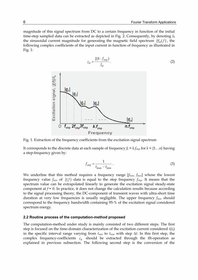
magnitude of this signal spectrum from DC to a certain frequency in function of the initial time-step sampled data can be extracted as depicted in Fig. 2. Consequently, by denoting I0 the sinusoidal current magnitude for generating the magnetic field spectrum 0( )H f , the following complex coefficients of the input current in function of frequency as illustrated in Fig. 1:
0
( )stepk
I k fc
I⋅
= . (2)
Fig. 1. Extraction of the frequency coefficients from the excitation signal spectrum
It corresponds to the discrete data at each sample of frequency fk = k.fstep for k = {1…n} having a step-frequency given by:
max min
1stepf
t t=
−. (3)
We underline that this method requires a frequency range [fmin, fmax] whose the lowest frequency value fmin of ( )I f -data is equal to the step frequency fstep. It means that the spectrum value can be extrapolated linearly to generate the excitation signal steady-state component at f = 0. In practice, it does not change the calculation results because according to the signal processing theory, the DC-component of transient waves with ultra-short time duration at very low frequencies is usually negligible. The upper frequency fmax should correspond to the frequency bandwidth containing 95-% of the excitation signal considered spectrum energy.
2.2 Routine process of the computation-method proposed
The computation-method under study is mainly consisted of two different steps. The first step is focused on the time-domain characterization of the excitation current considered i(tk) in the specific interval range varying from tmin to tmax with step ∆t. In this first step, the complex frequency-coefficients kc should be extracted through the fft-operation as explained in previous subsection. The following second step is the conversion of the

Computation of Transient Near-Field Radiated by Electronic Devices from Frequency Data
7
frequency-dependent magnetic- or H-field expressed by 00( , , , )H x y z f which is recorded at the point 0( , , )M x y z chosen arbitrarily, into a time-dependent data denoted by 0( , , , )H x y z t by using the ifft-operation. These points 0( , , )M x y z belong in the X-Y plane positioned at z = z0. In this case, the frequency range considered varying from fmin to fmax and the frequency step fstep of 0 0 0( ) ( , , , )H f H x y z f= must be well-synchronized with that of the excitation signal frequency coefficients ck. Under this condition, the time-dependent data desired
0( ) ( , , , )H t H x y z t= which is generated by the specific excitation signal i(t) can be calculated with the inverse fast Fourier transform (ifft) of the convolution product between
0( ) ( ) /c f I f I= and 0( )H f written as:
{ }0( ) [ ( ). ( )]H t e ifft c f H f= ℜ . (4)
with { }e xℜ represents the real part of the complex number x. Fig. 2 depicts the flow work highlighting the different operations to be fulfilled for the achievement of the transient EM-field computation-method proposed. This method enables to provide the time-dependent
Fig. 2. Flow work illustrating the transient H-field radiation computation-method proposed knowing the temporal range, tmin and tmax step Δt of the excitation signal i(tk) and also the frequency-dependent H-field 0( )H f (here the under bar indicates the complex variables)
Fourier Transform Applications
8
H-field here denoted as H(t) according to the arbitrary form of the excitation and also knowing the frequency-dependent H-field data in the frequency range starting from the lowest value to the upper frequency limit equal to the inverse of the time-step ∆t of the discrete data x(tk).
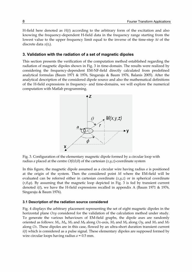
3. Validation with the radiation of a set of magnetic dipoles This section presents the verification of the computation method established regarding the radiation of magnetic dipoles shown in Fig. 3 in time-domain. The results were realized by considering the frequency-dependent EM-NF-field directly calculated from predefined analytical formulas (Baum 1971 & 1976, Singaraju & Baum 1976, Balanis 2005). After the analytical description of the considered dipole source and also the mathematical definitions of the H-field expressions in frequency- and time-domains, we will explore the numerical computation with Matlab programming.
Fig. 3. Configuration of the elementary magnetic dipole formed by a circular loop with radius a placed at the centre O(0,0,0) of the cartesian (x,y,z)-coordinate system
In this figure, the magnetic dipole assumed as a circular wire having radius a is positioned at the origin of the system. Then the considered point M where the EM-field will be evaluated can be referred either in cartesian coordinate (x,y,z) or in spherical coordinate (r,θ,φ). By assuming that the magnetic loop depicted in Fig. 3 is fed by transient current denoted i(t), we have the H-field expressions recalled in appendix A (Baum 1971 & 1976, Singaraju & Baum 1976).
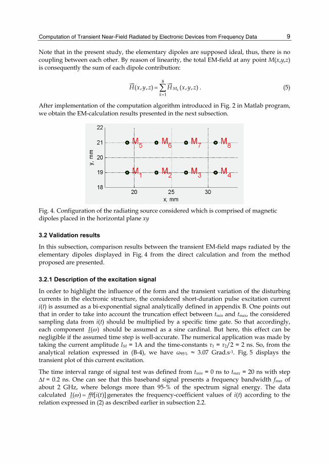
3.1 Description of the radiation source considered
Fig. 4 displays the arbitrary placement representing the set of eight magnetic dipoles in the horizontal plane Oxy considered for the validation of the calculation method under study. To generate the various behaviours of EM-field graphs, the dipole axes are randomly oriented as follows: M1, M4, M5 and M8 along Ox-axis, M2 and M6 along Oy, and M3 and M7 along Oz. These dipoles are in this case, flowed by an ultra-short duration transient current i(t) which is considered as a pulse signal. These elementary dipoles are supposed formed by wire circular loops having radius a = 0.5 mm.
Computation of Transient Near-Field Radiated by Electronic Devices from Frequency Data
9
Note that in the present study, the elementary dipoles are supposed ideal, thus, there is no coupling between each other. By reason of linearity, the total EM-field at any point M(x,y,z) is consequently the sum of each dipole contribution:
8
1( , , ) ( , , )kM
kH x y z H x y z
== ∑ . (5)
After implementation of the computation algorithm introduced in Fig. 2 in Matlab program, we obtain the EM-calculation results presented in the next subsection.
Fig. 4. Configuration of the radiating source considered which is comprised of magnetic dipoles placed in the horizontal plane xy
3.2 Validation results
In this subsection, comparison results between the transient EM-field maps radiated by the elementary dipoles displayed in Fig. 4 from the direct calculation and from the method proposed are presented.
3.2.1 Description of the excitation signal
In order to highlight the influence of the form and the transient variation of the disturbing currents in the electronic structure, the considered short-duration pulse excitation current i(t) is assumed as a bi-exponential signal analytically defined in appendix B. One points out that in order to take into account the truncation effect between tmin and tmax, the considered sampling data from i(t) should be multiplied by a specific time gate. So that accordingly, each component ( )I ω should be assumed as a sine cardinal. But here, this effect can be negligible if the assumed time step is well-accurate. The numerical application was made by taking the current amplitude IM = 1A and the time-constants τ1 = τ2/2 = 2 ns. So, from the analytical relation expressed in (B-4), we have ω95% ≈ 3.07 Grad.s-1. Fig. 5 displays the transient plot of this current excitation.
The time interval range of signal test was defined from tmin = 0 ns to tmax = 20 ns with step ∆t = 0.2 ns. One can see that this baseband signal presents a frequency bandwidth fmax of about 2 GHz, where belongs more than 95-% of the spectrum signal energy. The data calculated ( ) [ ( )]I fft i tω = generates the frequency-coefficient values of i(t) according to the relation expressed in (2) as described earlier in subsection 2.2.

Fourier Transform Applications
10
3.2.2 Discussions on the computed results
By considering the set of eight magnetic dipoles presented in Fig. 4 which are excited by the same pulse current plotted in Fig. 5 yields the H-field component (Hx, Hy and Hz) mappings depicted in Fig. 6 at the arbitrary time t0 = 2 ns and in the horizontal plane parallel to (Oxy) referenced z0 = 6.5 mm above the radiating source.
Fig. 5. Transient plot of the considered excitation current i(t)
Fig. 6. Maps of H-field components detected at the height z0 = 6.5 mm above the radiating source: (a) Hx, (b) Hy and (c) Hz obtained from the direct calculation

Computation of Transient Near-Field Radiated by Electronic Devices from Frequency Data
11
This height was arbitrarily chosen in order to generate a significant NF effect in the considered frequency range. The dimensions of the mapping plane were set at Lx = 110 mm and Ly = 100 mm with space-resolution equal to ∆x = ∆y = 2 mm. First, by using the harmonic expressions of the magnetic field components, the maps of the frequency-dependent H-field are obtained from fmin = 0.05 GHz to fmax = 2.50 GHz with step ∆f = 0.05 GHz. Fig. 7 represents the corresponding mappings of the H-field component magnitudes at f0 = 2 GHz.
Fig. 7. Maps of H-field components magnitude obtained at the frequency f0 = 2 GHz: (a) Hx, (b) Hy and (c) Hz directly calculated from expressions (A-8), (A-9) and (A-10)
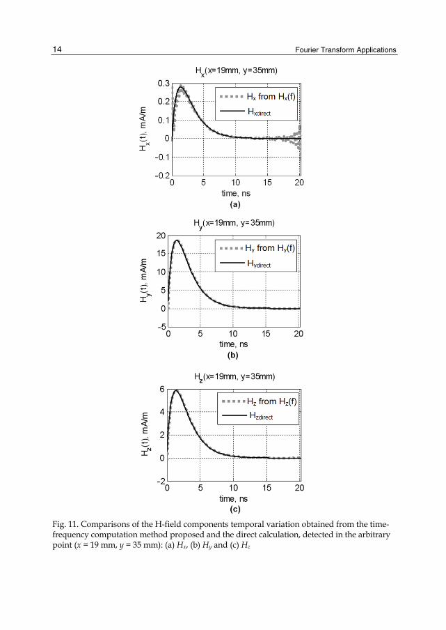
After the Matlab program implementation of the algorithm indicated by the flow chart schematized in Fig. 2, the results shown in Figs. 8(a)-(d) are obtained via the combination of the frequency-dependent data of the H-field components associated to the frequency-coefficients of the excitation signal plotted in Fig. 5. One can see that the EM-maps presenting the same behaviors as those obtained via the direct calculations displayed in Fig. 6 were established. In addition, we compare also as illustrated in Fig. 9 the modulus of the H-fields from the method under study and from the 3D EM Field Simulator - CST (Computer Simulation Technology). Furthermore, as evidenced by Figs. 10(a)-(c), very good correlation between the profiles of the H-field components detected in the vertical cut-plane along Oy and localized at x = 23 mm was observed. To get further insight about the time-dependent representation of the H-field components, curves showing the variations of Hx(t), Hy(t) and Hz(t) at the arbitrary point chosen of the mapping plane having coordinates (x = 19 mm, y = 35 mm) are plotted in Figs. 11(a)-(c).

Fourier Transform Applications
12
As results, once again, we can find that the H-field components from the frequency data fit very well the direct calculated ones. As aforementioned, due to the truncation effects, the Hx-component presents a slight divergence at the ending time of the signal. This is particularly due to the numerical noises at the very low value of the EM field as the case of the x-component which is absolutely twenty times less than the two other components.
In order to prove in more realistic way the relevance of the investigated method, one proposes to treat the radiation of concrete electronic devices in the next section.
Fig. 8. Maps of H-field components calculated from the time-frequency computation method proposed for z0 = 6.5 mm: (a) Hx, (b) Hy, (c) Hz
Fig. 9. Comparison of H-field maps modulus |H|(t0 = 2 ns) obtained from the direct formulae (in left) and from the time-frequency computation method proposed for z0 = 6.5 mm

Computation of Transient Near-Field Radiated by Electronic Devices from Frequency Data
13
Fig. 10. Comparisons of the H-field component profiles obtained from the time-frequency computation method proposed and the direct calculation, detected in the vertical cut-plane x = 23 mm: (a) Hx, (b) Hy and (c) Hz
Fourier Transform Applications
14
Fig. 11. Comparisons of the H-field components temporal variation obtained from the time-frequency computation method proposed and the direct calculation, detected in the arbitrary point (x = 19 mm, y = 35 mm): (a) Hx, (b) Hy and (c) Hz

Computation of Transient Near-Field Radiated by Electronic Devices from Frequency Data
15
4. Application with the Transient NF emitted by a microstrip device proof-of-concept To get further insight about the feasibility of the computation method under study, let us examine the transient EM-wave emitted by an example of more realistic microwave device. This latter was designed with the standard 3-D EM-tools HFSS for generating the frequency-dependent data which is used for the determination of transient H-NF. Then, the simulation with CST microwave studio (MWS) was performed for the computation of the reference H-NF mappings in time-domain. As realistic and concrete demonstrator, a low-pass Tchebychev filter implemented in planar microstrip technology was designed. Its layout top view including the geometrical dimensions is represented in Fig. 12(a).
This device was printed on the FR4-epoxy substrate having relativity permittivity εr = 4.4, thickness h = 1.6 mm and etched Cu-metal thickness t = 35 µm. The cut cross section of this microwave circuit is pictured in Fig. 12(b).
(a)
(b)
Fig. 12. (a) Top view of the CST design of the under test low-pass microstrip filter (b) Cross-section cut of the under test microstrip filter with metallization thickness t = 35 µm and dielectric substrate height h = 1.6 mm
After simulations, we realize the results obtained and discussed in next subsections.

Fourier Transform Applications
16
4.1 CST-computation results
The low-pass filter under test was simulated with CST MWS in the time interval range delimited by tmin = 0 ns and tmax = 20 ns with step ∆t = 0.2 ns. Therefore, the magnetic-field maps are presented in Fig. 13. These curves are recorded at the arbitrary instant time t0 = 2 ns. Note that this structure was excited by the input transient current plotted in Fig. 5. It results the graphs of H-field components displayed in Fig. 13.
Fig. 13. Maps of transient H-field components detected at t = 2 ns: (a) Hx, (b) Hy and (c) Hz computed from the commercial tool CST
Computation of Transient Near-Field Radiated by Electronic Devices from Frequency Data
17
Similar to the previous section, these H-field components were mapped in the horizontal plane placed at the height z0 = 6 mm above the bottom surface of the considered filter and delimited by -38 mm < x < 38 mm and -24 mm < y < 24 mm with space-step ∆x = ∆y = 2 mm. By using the frequency-dependent data convoluted with the excitation test signal, we will present next that we can regenerate these transient H-field maps.
4.2 Analysis of the results obtained from the transient field computation method proposed
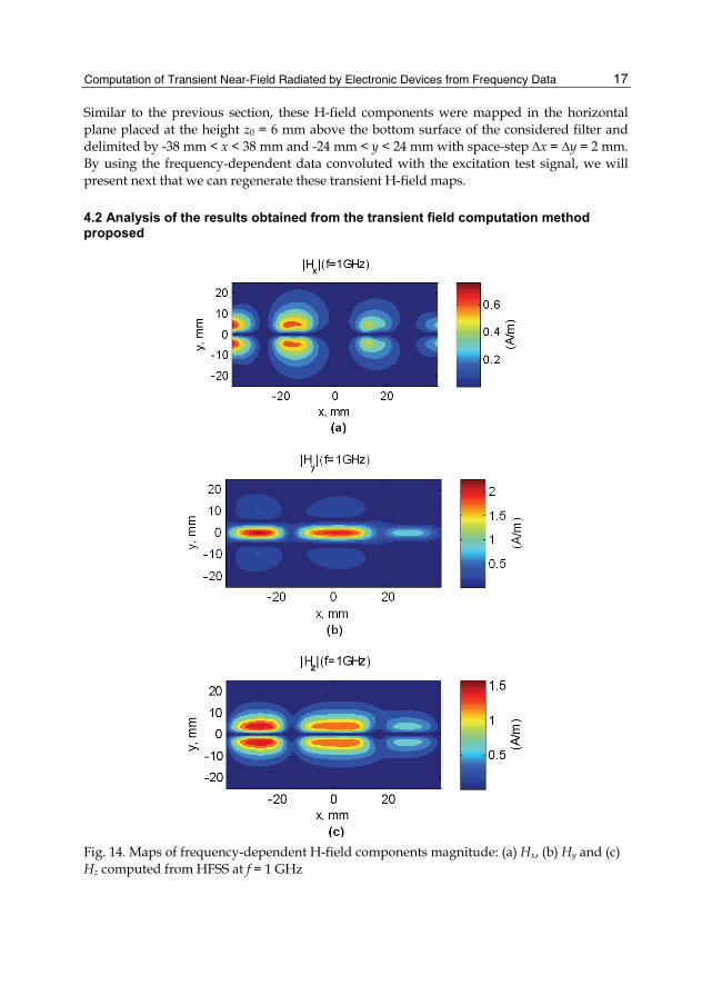
Fig. 14. Maps of frequency-dependent H-field components magnitude: (a) Hx, (b) Hy and (c) Hz computed from HFSS at f = 1 GHz
Fourier Transform Applications
18
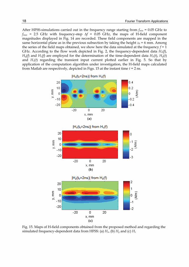
After HFSS-simulations carried out in the frequency range starting from fmin = 0.05 GHz to fmax = 2.5 GHz with frequency-step ∆f = 0.05 GHz, the maps of H-field component magnitudes displayed in Fig. 14 are recorded. These field components are mapped in the same horizontal plane as in the previous subsection by taking the height z0 = 6 mm. Among the series of the field maps obtained, we show here the data simulated at the frequency f = 1 GHz. According to the flow work depicted in Fig. 2, the frequency-dependent data Hx(f), Hy(f) and Hz(f) are employed for the determination of the time-dependent data Hx(t), Hy(t) and Hz(t) regarding the transient input current plotted earlier in Fig. 5. So that by application of the computation algorithm under investigation, the H-field maps calculated from Matlab are respectively, depicted in Figs. 15 at the instant time t = 2 ns.
Fig. 15. Maps of H-field components obtained from the proposed method and regarding the simulated frequency-dependent data from HFSS: (a) Hx, (b) Hy and (c) Hz
Computation of Transient Near-Field Radiated by Electronic Devices from Frequency Data
19
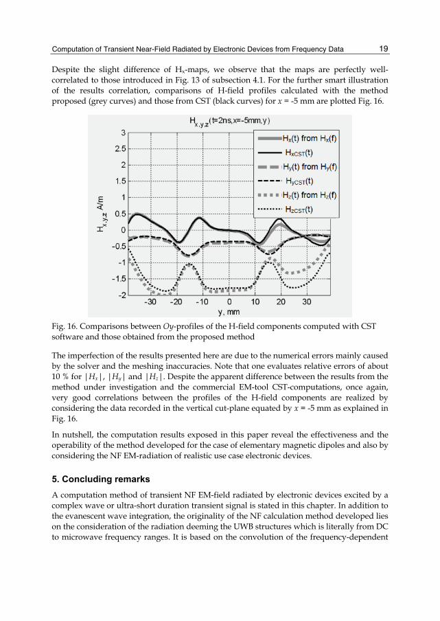
Despite the slight difference of Hx-maps, we observe that the maps are perfectly well-correlated to those introduced in Fig. 13 of subsection 4.1. For the further smart illustration of the results correlation, comparisons of H-field profiles calculated with the method proposed (grey curves) and those from CST (black curves) for x = -5 mm are plotted Fig. 16.
Fig. 16. Comparisons between Oy-profiles of the H-field components computed with CST software and those obtained from the proposed method
The imperfection of the results presented here are due to the numerical errors mainly caused by the solver and the meshing inaccuracies. Note that one evaluates relative errors of about 10 % for |Hx|, |Hy| and |Hz|. Despite the apparent difference between the results from the method under investigation and the commercial EM-tool CST-computations, once again, very good correlations between the profiles of the H-field components are realized by considering the data recorded in the vertical cut-plane equated by x = -5 mm as explained in Fig. 16.
In nutshell, the computation results exposed in this paper reveal the effectiveness and the operability of the method developed for the case of elementary magnetic dipoles and also by considering the NF EM-radiation of realistic use case electronic devices.
5. Concluding remarks A computation method of transient NF EM-field radiated by electronic devices excited by a complex wave or ultra-short duration transient signal is stated in this chapter. In addition to the evanescent wave integration, the originality of the NF calculation method developed lies on the consideration of the radiation deeming the UWB structures which is literally from DC to microwave frequency ranges. It is based on the convolution of the frequency-dependent

Fourier Transform Applications
20
EM-wave data with a transient excitation pulse current. A methodological analysis was made by taking into account a complex waveform of the transient pulse signal exciting the radiation source structure considered. It was explained how the frequency-bandwidth of the frequency-dependent baseband EM-field must be chosen according to the excitation current considered.
In order to demonstrate the relevance of the method investigated, it was first, implemented into Matlab program and then, applied to the determination of the H-field radiated by a microwave circuit in UWB. As consequence, the feasibility of the method was verified with two types of structures. First, with the semi-analytical calculation implemented in Matlab by considering the frequency- and time-dependent expressions of the magnetic NF radiated by a set of magnetic dipoles, an excellent agreement with the results from the calculation method developed were found. Then, further more practical analysis was performed with the determination of transient H-NF from the frequency-dependent data computed with a standard commercial 3-D EM-tool. For this second test, the H-NF emitted by a low-pass planar microstrip filter was treated. For both cases, the excitation current injected to the structures was assumed as an ultra-short transient pulse having half-bandwidth lower than 5 ns which presents a baseband frequency spectrum with bandwidth of about 2.5 GHz from DC. With the examples of complex structures tested, very good agreement between the transient H-field component maps and profiles was realized from the method proposed and those directly calculated from the well-known standard tools and from classical mathematical EM-formulae.
It is interesting to point up that the NF computation method introduced in this chapter is advantageous in terms of:
1. Simplicity of the EM-field maps determination for any waveform of transient excitation even with ultra-short duration which is very hard to simulate with most of commercial simulation tools. The method developed can be used for the determination of the NF maps in time-domain which is practically very difficult to measure in the realistic contexts.
2. It is flexible for various types of excitation signals which can be expressed analytically and also from the realistic use case of disturbing signal generally met in EMC area (Wiles 2003, Liu, K. 2011, Hubing 2011).
3. It can be adapted also to different forms of electrical and electronic structures for low- and high-frequency applications. Globally speaking, it offers a possibility to work in UWB from DC to unlimited upper frequency limit.
4. One can achieve significant EM-field measurement in very short time-duration with base band measured data in wide bandwidth.
However, its main drawback is the limitation in term of time step which depends on the frequency range of the initial frequency-data considered and also the necessity of powerful computer for the achievement of high accurate results.
In the next step of this work, we plane to extend this method to transpose in time-domain the modelling of EM-radiation with the optimized association of elementary dipoles (Vives-Gilabert et al. 2009, Fernández-López et al. 2009). Then, we are hopeful that the method developed in this chapter is very helpful for EMC/EMI investigations of modern electrical/electronic systems as the case of hybrid vehicle embedded circuits (Vye 2011,

Computation of Transient Near-Field Radiated by Electronic Devices from Frequency Data
21
Tröscher 2011, Kopp 2011) where the transient NF effects are susceptible to disturb the system functioning.
6. Appendix This appendix contains two parts of theoretical parts concerning the transient NF radiated by the elementary magnetic dipoles (Baum 1971 & 1976, Singaraju & Baum 1976, Ravelo et al. 2011a & 2011b, Lui Y. et al. 2011a & 2011b) and the bi-exponential signal processing.
6.1 Appendix A: Analytical study of the magnetic dipole radiation in time-domain
By definition, the magnetic dipole moment of the elementary circular loop shown earlier in Fig. 3 (see section 3) is written as:
( , ) ( ) ( ) zMp r t p t r uδ= ⋅ ⋅ , (A-1)
with r is the distance between the dipole centre and the point M(r,θ,φ) as shown in Fig. 3. By analogy with the definition of the time-variant vector established by Hertz in 1892 (Hertz 1892), the H-field components in the spherical coordinate system:
( , , , ) ( , , , ) ( , , , )rrH H r t u H r t u H r t uθ ϕθ ϕθ ϕ θ ϕ θ ϕ= + + , (A-2)
are expressed as:
2
( ) ( )cos( ) 1( , , , )2r
p pH r tr v trτ τθθ ϕ
π∂⎡ ⎤= +⎢ ⎥∂⎣ ⎦
, (A-3)
2
2 2 2( ) ( ) ( )sin( ) 1( , , , )
4p p prH r t
r v tr v tθτ τ τθθ ϕ
π
⎡ ⎤∂ ∂= + +⎢ ⎥
∂ ∂⎢ ⎥⎣ ⎦, (A-4)
( , , , ) 0H r tϕ θ ϕ = , (A-5)
where v is the wave-velocity, and τ is the time delayed variable which is defined as /t r vτ = − . One underlines that the magnetic dipole is also an Hertzian dipole so that
( , ) / 0i r t r∂ ∂ = . In the frequency domain, the spherical coordinate of the H-field component formulas radiated by the magnetic dipole pictured in Fig. 3 which is supposed flowed by an harmonic current with amplitude IM denoted:
2( ) j ft j tM MI f I e I eπ ω− −= = , (A-6)
are written as (Balanis 2005):
( )2
3( , , , ) 1 cos( )2
jkrMr
I aH r f jkr er
θ ϕ θ −= + , (A-8)
2
2 23
sin( )( , , , ) (1 )4
jkrMI aH r f jkr k r erθ
θθ ϕ −= + − , (A-9)
Fourier Transform Applications
22
( , , , ) 0H r fϕ θ ϕ = , (A-10)
where j is the complex number 1− and the real 2 /k f vπ= expresses the wave number at the considered frequency f. Then, through the classical relationship between the spherical and cartesian coordinate systems, one can determine easily the expressions of the components Hx, Hy and Hz.
6.2 Appendix B: Spectrum analysis of bi-exponential signal
A bi-exponential form signal with parameters τ1 and τ2 is analytically expressed as:
1 2/ /( ) ( )t tMi t I e eτ τ− −= − . (B-1)
The analytical Fourier transform expression of this current is written as:
1 2
1 2( ) ( )
1 1MI Ij jτ τωωτ ωτ
= −+ +
, (B-2)
with ω is the angular frequency. This yields the signal frequency spectrum formulation expressed as:
1 22 2 2 21 2
( )(1 )(1 )
MI Iτ τ
ωτ ω τ ω
−=
+ +. (B-3)
To achieve at least 95-% of excitation signal spectrum energy, the frequency-data should be recorded in baseband frequency range with angular frequency bandwidth equal to:
2 2 2 2 2 2 21 2 1 2 1 2
95%1 2
( ) 16002
τ τ τ τ τ τω
τ τ
− + − −= . (B-4)
7. Acknowledgment Acknowledgement is made to EU (European Union) and Upper Normandy region for the support of these researches. These works have been implemented within the frame of the “Time Domain Electromagnetic Characterisation and Simulation for EMC” (TECS) project No 4081 which is part-funded by the Upper Normandy Region and the ERDF via the Franco-British Interreg IVA programme.
8. References Adada, M. (2007). High-Frequency Simulation Technologies-Focused on Specific High-
Frequency Design Applications. Microwave Engineering Europe, (Jun. 2007), pp. 16-17
Agilent EEsof EDA. (2008). Overview: Electromagnetic Design System (EMDS), (Sep. 2008) [Online]. Available from:
http://www.agilent.com/find/eesof-emds

Computation of Transient Near-Field Radiated by Electronic Devices from Frequency Data
23
Ansoft corporation. (2006). Simulation Software: High-performance Signal and Power Integrity, Internal Report
ANSYS, (2009). Unparalleled Advancements in Signal- and Power-Integrity, Electromagnetic Compatibility Testing, (Jun. 16 2009) [Online]. Available from:
http://investors.ansys.com/ Archambeault, B.; Brench, C. & Connor, S. (2010). Review of Printed-Circuit-Board Level
EMI/EMC Issues and Tools. IEEE Trans. EMC, (May 2010), Vol. 52, No.2, pp. 455-461, ISSN 0018-9375
Balanis, C. A. (2005). Antenna Theory: Analysis and Design, in Wiley, (3rd Ed.), 207–208, New York, USA, ISBN: 978-0-471-66782-7
Barriere, P.-A.; Laurin, J.-J. & Goussard, Y. (2009). Mapping of Equivalent Currents on High-Speed Digital Printed Circuit Boards Based on Near-Field Measurements. IEEE Trans. EMC, (Aug. 2009), Vol.51, No.3, pp. 649 - 658, ISSN 0018-9375
Baudry, D.; Arcambal, C.; Louis, A.; Mazari, B. & Eudeline, P. (2007). Applications of the Near-Field Techniques in EMC Investigations. IEEE Trans. EMC, (Aug. 2007), Vol.49, No.3, pp. 485-493, ISSN 0018-9375
Baum, C. E. (1971). Some Characteristics of Electric and Magnetic Dipole Antennas for Radiating Transient Pulses, Sensor and Simulation Note 405, 23 Jan. 71
Baum, C. E. (1976). Emerging Technology for Transient and Broad-Band Analysis and Synthesis of Antennas and Scaterrers, Interaction Note 300, Proceedings of IEEE, (Nov. 1976), pp. 1598-1616
Braun, S.; Gülten, E.; Frech, A. & Russer, P. (2009). Automated Measurement of Intermittent Signals using a Time-Domain EMI Measurement System, Proceedings of IEEE Int. Symp. EMC, pp. 232-235, ISBN 978-1-4244-4266-9, Austin, Texas (USA), Aug. 17-21 2009
Chew, W. C. & Kong, J. A. (1981). Electromagnetic field of a dipole on a two-layer earth. Geophysics, (Mar. 1981), Vol. 46, No. 3, pp. 309-315
Cicchetti, R. (1991). Transient Analysis of Radiated Field from Electric Dipoles and Microstrip Lines. IEEE Trans. Ant. Prop., (Jul. 1991), Vol.39, No.7, pp. 910-918, ISSN 0018-926X
Edwards, R. S.; Marvin, A. C. & Porter, S. J. (2010). Uncertainty Analyses in the Finite-Difference Time-Domain Method. IEEE Trans. EMC, (Feb. 2010), Vol.52, No.1, pp. 155-163, ISSN 0018-9375
Fernández-López, P.; Arcambal, C.; Baudry, D.; Verdeyme, S. & Mazari, B. (2009). Radiation Modeling and Electromagnetic Simulation of an Active Circuit, Proceedings of EMC Compo 09, Toulouse, France, Nov. 17-19 2009
Hertz, H. R. (1892). Untersuchungen ueber die Ausbreitung der Elektrischen Kraft (in German). Johann Ambrosius Barth, Leipzig, Germany, ISBN-10: 1142281167/ISBN-13: 978-1142281168
Hubing, T. (2011). Ensuring the Electromagnetic Compatibility of Safety Critical Automotive Systems. Invited Plenary Speaker at the 2011 APEMC, Jeju, South-Korea, May 2011
Jauregui, R.; Pous, M.; Fernández, M. & Silva, F. (2010). Transient Perturbation Analysis in Digital Radio, Proceedings of IEEE Int. Symp. EMC, pp. 263-268, ISBN 978-1-4244-6307-7, Fort Lauderdale, Florida (USA), Jul. 25-30 2010

Fourier Transform Applications
24
Jauregui, R.; Riu, P. I. & Silva, F. (2010). Transient FDTD Simulation Validation, Proceedings of IEEE Int. Symp. EMC, pp. 257-262, ISBN 978-1-4244-6305-3, Fort Lauderdale, Florida (USA), Jul. 25-30 2010
Jun-Hong, W.; Lang, J. & Shui-Sheng, J. (1997). Optimization of the Dipole Shapes for Maximum Peak Values of the Radiating Pulse, Proceedings of IEEE Tran. Ant. Prop. Society Int. Symp., Vol.1, pp. 526-529, Montreal, Que., Canada, 13-18 Jul 1997, ISBN 0-7803-4178-3
Kopp, M. (2011). Automotive EMI/EMC Simulation. Microwave Journal, (Jul. 2011), Vol.54, No.7, pp. 24-32
Lakhtakiaa, A.; Varadana, V. K. & Varadana, V. V. (1987). Time-Harmonic and Time-Dependent Radiation by Bifractal Dipole Arrays. Int. J. Electronics, (Dec. 1987), Vol.63, No.6, pp. 819-824, DOI:10.1080/00207218708939187
Liu, K. (2011). An Update on Automotive EMC Testing. Microwave Journal, (Jul. 2011), Vol.54, No.7, pp. 40-46
Liu, L.; Cui, X. & Qi, L.. (2009). Simulation of Electromagnetic Transients of the Bus Bar in Substation by the Time-Domain Finite-Element Method. IEEE Trans. EMC, (Nov. 2009), Vol.51, No.4, pp. 1017-1025, ISSN 0018-9375
Liu, Y.; Ravelo, B.; Jastrzebski, A. K. & Ben Hadj Slama, J. (2011). Calculation of the Time Domain z-Component of the EM-Near-Field from the x- and y-Components, Accepted for communication in EuMC 2011, Manchester, UK, Oct. 9-14 2011
Liu, Y.; Ravelo, B.; Jastrzebski, A. K. & Ben Hadj Slama, J. (2011). Computational Method of Extraction of the 3D E-Field from the 2D H-Near-Field using PWS Transform, Accepted for communication in EMC Europe 2011, York, UK, Sep. 26-30 2011
North East Systems Associates (NESA), (2010). RJ45 Interconnect Signal Integrity, (2010 CST Computer Simulation Technology AG.) [Online]. Available from:
http://www.cst.com/Content/Applications/Article/Article.aspx?id=243 Ordas, T.; Lisart, M.; Sicard, E.; Maurine, P. & Torres, L. (2009). Near-Field Mapping
System to Scan in Time Domain the Magnetic Emissions of Integrated Circuits, Proceedings of PATMOS’ 08: Int. Workshop on Power and Timing Modeling Optimization and Simulation, Ver. 1-11, Lisbon, Portugal, Sep. 10-12 2008, ISBN 978-3-540-95947-2
Rammal, R.; Lalande, M.; Martinod, E.; Feix, N.; Jouvet, M.; Andrieu, J. & Jecko, B. (2009). Far Field Reconstruction from Transient Near-Field Measurement Using Cylindrical Modal Development, Int. J. Ant. Prop., Hindawi, Vol. 2009, Article ID 798473, 7 pages, doi:10.1155/2009/798473
Ravelo, B. (2010). E-Field Extraction from H-Near-Field in Time-Domain by using PWS Method. PIER B Journal, Vol.25, pp. 171-189, doi:10.2528
Ravelo, B.; Liu, Y.; Louis, A. & Jastrzebski, A. K. (2011). Study of high-frequency electromagnetic transients radiated by electric dipoles in near-field. IET Microw. Antennas Propag., (Apr. 2011), Vol. 5, No, 6, pp 692 - 698, ISSN 1751-8725
Ravelo, B.; Liu, Y. & Slama, J. B. H. (2011). Time-Domain Planar Near-Field/Near-Field Transforms with PWS Method. Eur. Phys. J. Appl. Phys. (EPJAP), (Feb. 2011), Vol.53, No.1, 30701-pp. 1-8, doi: 10.1051/epjap/2011100447
Computation of Transient Near-Field Radiated by Electronic Devices from Frequency Data
25
Rioult, J.; Seetharamdoo, D. & Heddebaut, M. (2009). Novel Electromagnetic Field Measuring Instrument with Real-Time Visualization, Proceedings of IEEE Int. Symp. EMC, pp. 133-138, ISBN 978-1-4244-4266-9, Austin, Texas (USA), Aug. 17-21 2009
Schantz, H. G. (2001). Electromagnetic Energy around Hertzian Dipoles. IEEE Tran. Ant. Prop. Magazine, (Apr. 2001), Vol.43, No.2, pp. 50-62, ISBN 9780470688625
Selin, V. I. (2001). Asymptotics of the Electromagnetic Field Generated by a Point Source in a Layered Medium. Computational Mathematics and Mathematical Physics, Vol.41, No.6, pp. 915-939, ISSN 0965-5425
Shi, J.; Cracraft, M. A.; Zhang J. & DuBroff, R. E. (1989). Using Near-Field Scanning to Predict Radiated Fields, Proceedings of IEEE Ant. Prop. Int. Symp., Vol.3, pp. 1477-1480, San Jose, CA (USA)
Singaraju, B. K. & Baum, C. E. (1976). A Simple Technique for Obtaining the Near Fields of Electric Dipole Antennas from Their Far Fields, Sensor and Simulation Note 213, Mar. 76
Smagin, S. I. & Mazalov, V. N. (2005). Calculation of the Electromagnetic Fields of Dipole Sources in Layered Media. Doklady Physics, (Apr. 2005), Vol.50, No.4, pp. 178-183, DOI:10.1134/1.1922556
Song, J. & Chen, K.-M. (1993). Propagation of EM Pulses Excited by an Electric Dipole in a Conducting Medium. IEEE Tran. Ant. Prop., (Oct. 1993), Vol.41, No.10, pp. 1414-1421, ISSN 0018-926X
Song, Z.; Donglin, S.; Duval, F.; Louis, A. & Fei, D. (2010). A Novel Electromagnetic Radiated Emission Source Identification Methodology. Proceedings of Asia-Pacific Symposium on EMC, Pekin (China), Apr. 12-16 2010, ISBN 978-1-4244-5621-5
Sten, J. C.-E. & Hujanen, A. (2006). Aspects on the Phase Delay and Phase Velocity in the Electromagnetic Near-Field. PIER Journal, Vol. 56, pp. 67-80, doi:10.2528
Tröscher, M. (2011). 3D EMC/EMI Simulation of Automotive Multimedia Systems. Microwave Journal, (Jul. 2011), Vol.54, No.7, pp. 34-38
Vives-Gilabert, Y.; Arcambal, C.; Louis, A.; Daran, F.; Eudeline, P. & Mazari, B. (2007). Modeling Magnetic Radiations of Electronic Circuits using Near-Field Scanning Method. IEEE Tran. EMC, (May 2007), Vol.49, No.2, pp. 391-400, ISSN 0018-9375
Vives-Gilabert, Y.; Arcambal, C.; Louis, A.; Eudeline, P. & Mazari, B. (2009). Modeling Magnetic Emissions Combining Image Processing and an Optimization Algorithm. IEEE Tran. EMC, (Nov. 2009), Vol.51, No.4, pp. 909-918, ISSN 0018-9375
Vye, D. (2011). EMI by the Dashboard Light. Microwave Journal, (Jul. 2011), Vol.54, No.7, pp. 20-23
Wiles, M. (2003). An Overview of Automotive EMC Testing Facilities, Proceedings of Automotive EMC Conf. 2003, Milton Keynes, UK, Nov. 6 2003
Winter, W. & Herbrig, M. (2009). Time Domain Measurement in Automotive Applications, Proceedings of IEEE Int. Symp. EMC, pp. 109-115, ISBN 9781424442669, Austin, Texas (USA), Aug. 17-21 2009
Xie, L. & Lei, Y. (2009). Transient Response of a Multiconductor Transmission Line With Nonlinear Terminations Excited by an Electric Dipole. IEEE Trans. EMC, (Aug. 2009), Vol.51, No.3, pp. 805-810, ISSN 0018-9375

Fourier Transform Applications
26
Yang, T.; Bayram, Y. & Volakis, J. L. (2010). Hybrid Analysis of Electromagnetic Interference Effects on Microwave Active Circuits Within Cavity Enclosures. IEEE Trans. EMC, (Aug. 2010), Vol.52, No.3, pp. 745-748, ISSN 0018-9375

0
Impulse-Regime Analysis of NovelOptically-Inspired Phenomena at Microwaves
J. Sebastian Gomez-Diaz1, Alejandro Alvarez-Melcon1,Shulabh Gupta2 and Christophe Caloz2
1Universidad Politécnica de Cartagena2École Polytechnique de Montréal
1Spain2Canada
1. Introduction
The ever increasing of needs for high data-rate wireless system is currently producing a shiftfrom narrow-band radio towards ultra-wideband (UWB) radio operation [see Ghavami et al.(2007)]. Novel microwave tools, concepts, phenomena and direct applications must bedeveloped to meet this demand. While the past decades have been focused on the "magnitudeengineering" and filter design [see Pozar (2005)], there is a renewed interest in the "dispersionengineering". In the dispersion engineering approach, the phase is engineered to met variousspecifications within a given frequency range, so as to process signals in real time.
In this context, the development of electromagnetic metamaterials over the last years [seeCaloz & Itoh (2006) or Marques et al. (2008)], with their intrinsically dispersive nature andsubsequent impulse-regime properties, may provide novel and original solutions (see Fig. 1).Metamaterials can easily be synthesized in planar technology under the form of compositeright/left-handed (CRLH) transmission lines (TLs), using non-resonant [see Caloz & Itoh(2006)] or resonant [see Duran-Sindreu et al. (2009)] approaches. These structures haveprovided novel and exciting applications, such as multi-band components, diplexers,couplers, phase-shifters, power-dividers or antennas with enhanced features, to mentionjust a few [see Caloz (2009) or Eleftheriades (2009) for a recent review]. However, CRLHstructures have mostly been analyzed in the harmonic regime to date, and therefore only afew impulse-regime components and systems have been proposed so far. An example ofthese applications is the tunable pulse delay line presented in in Abielmona et al. (2007).
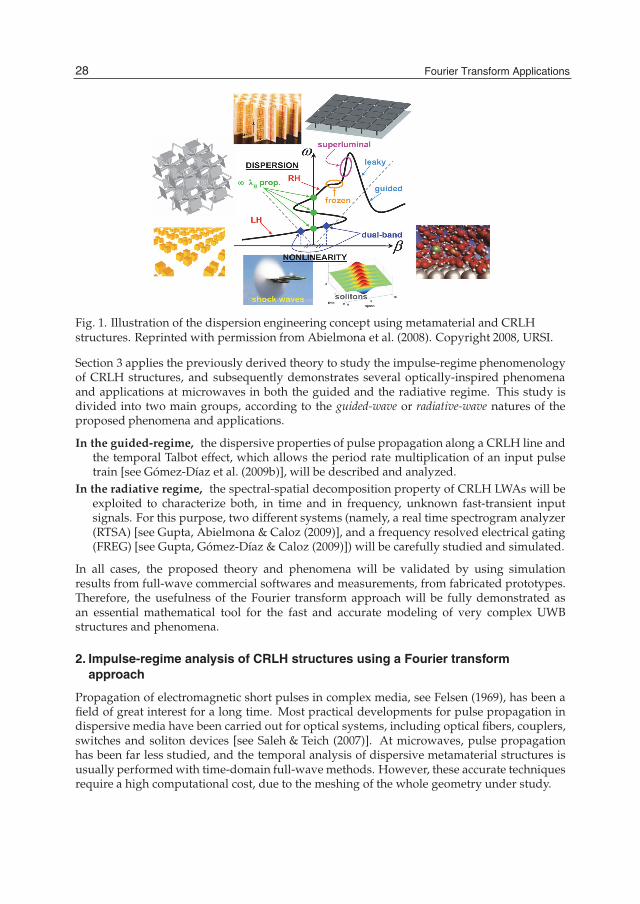
In this chapter, we present recent advances based on Fourier transformation techniques tomodel dispersive UWB phenomena and far-field radiation from complex CRLH structures.Section 2 first employs inverse Fourier transforms to study pulse propagation along thistype of medium. Then, a Fourier transform approach is applied to the current which flowsalong the CRLH line, accurately retrieving the time-domain far-field radiation of the structure[which behaves as a leaky-wave antenna, (LWA)]. The main advantages of the proposedtechniques are the easy treatment of complex CRLH structures, a deep insight into the physicsof the phenomena, and an accurate and a fast computation, which avoids the time-consuminganalysis required by completely numerical simulations.
2
2 Will-be-set-by-IN-TECH
Fig. 1. Illustration of the dispersion engineering concept using metamaterial and CRLHstructures. Reprinted with permission from Abielmona et al. (2008). Copyright 2008, URSI.
Section 3 applies the previously derived theory to study the impulse-regime phenomenologyof CRLH structures, and subsequently demonstrates several optically-inspired phenomenaand applications at microwaves in both the guided and the radiative regime. This study isdivided into two main groups, according to the guided-wave or radiative-wave natures of theproposed phenomena and applications.
In the guided-regime, the dispersive properties of pulse propagation along a CRLH line andthe temporal Talbot effect, which allows the period rate multiplication of an input pulsetrain [see Gómez-Díaz et al. (2009b)], will be described and analyzed.
In the radiative regime, the spectral-spatial decomposition property of CRLH LWAs will beexploited to characterize both, in time and in frequency, unknown fast-transient inputsignals. For this purpose, two different systems (namely, a real time spectrogram analyzer(RTSA) [see Gupta, Abielmona & Caloz (2009)], and a frequency resolved electrical gating(FREG) [see Gupta, Gómez-Díaz & Caloz (2009)]) will be carefully studied and simulated.
In all cases, the proposed theory and phenomena will be validated by using simulationresults from full-wave commercial softwares and measurements, from fabricated prototypes.Therefore, the usefulness of the Fourier transform approach will be fully demonstrated asan essential mathematical tool for the fast and accurate modeling of very complex UWBstructures and phenomena.
2. Impulse-regime analysis of CRLH structures using a Fourier transformapproach
Propagation of electromagnetic short pulses in complex media, see Felsen (1969), has been afield of great interest for a long time. Most practical developments for pulse propagation indispersive media have been carried out for optical systems, including optical fibers, couplers,switches and soliton devices [see Saleh & Teich (2007)]. At microwaves, pulse propagationhas been far less studied, and the temporal analysis of dispersive metamaterial structures isusually performed with time-domain full-wave methods. However, these accurate techniquesrequire a high computational cost, due to the meshing of the whole geometry under study.
28 Fourier Transform Applications
Impulse-Regime Analysis of Novel Optically-Inspired Phenomena at Microwaves 3
In this section, a general time-domain Green’s function approach is presented for theanalysis of pulse propagation in electrically thin CRLH TLs. This method is based on thetransient analysis of 1D transmission lines [see Paul (2007)] combined for the first time withCRLH TL concepts introduced in Caloz & Itoh (2006). With this equivalent transmissionline simplification of the geometry, the Green’s functions are available in closed-form, anddirectly correspond to the voltages and currents along the transmission line. The mainadvantages of this approach are the unconditional stability and fast computation, due to thecontinuous treatment of time, and the insight into the physical phenomena provided by theGreen’s functions. Subsequently, the method is extended to analyze impulse-regime CRLHleaky-wave antennas. The approach is based on the use of the time-domain current whichflows along the structure to compute the far-field radiation of the antenna. This technique isespecially appropriate to characterize complex radiated-wave UWB phenomena and devices,as it will be demonstrated in Section 3.
2.1 Composite right/left-handed structures
The introduction of metamaterials [see Caloz & Itoh (2006) or Marques et al. (2008)] in the lastdecade has paved the road to the development of new devices and applications based on thenovel fundamental features and phenomena associated to this type of media. Among the mostuseful metamaterials, one can find the CRLH transmission lines [see Caloz & Itoh (2006)].This type of transmission lines, which are inherently nonresonant and low-loss, can be easilyimplemented in planar technology (such as microstrip or coplanar waveguide, for instance)and provides a practical realization of electromagnetic metamaterials. As any metamaterial,CRLH TLs are generally periodic structures formed by the repetition of unit-cells (an exampleof this type of cells is shown in Fig. 2) whose size, p, must fulfill the condition p � λg(where λg is the guided wavelength) ir order to emulate an effectively homogeneous material.A powerful method to analyze these metamaterial lines is the TL approach, presented inCaloz & Itoh (2006), which employs an ABCD-matrix technique of periodically arrangedunit-cells to model the artificial transmission line (see Fig. 3) and to determine its wavepropagation characteristics (such as propagation constant or Bloch impedances, see Fig. 4).
There are many examples of interesting and groundbreaking applications of planar TLmetamaterials at microwaves, such as for instance multi-band components, filters anddiplexers, couplers, power-dividers, phase-shifters, lenses, or backfire to endfire leaky-waveantennas. A review of these and much more applications and devices can be found inmetamaterials textbooks, such as in Eleftheriades & Balmain (2005), in Caloz & Itoh (2006),or in Marques et al. (2008). Note that all previously mentioned and most of metamaterialsapplications operate in the harmonic regime up to now, and they have been designed fornarrow-band components and systems (even though some of them may support a multi-bandoperation).
2.2 Impulse regime analysis of CRLH transmission lines
Many media, ranging from traditional purely right-handed materials to recent CRLHmetamaterials [see Caloz & Itoh (2006)], can be advantageously analyzed by the transmissionline theory described in Pozar (2005). So far, this theory has been applied mostly in theharmonic regime, where Green’s functions for both the voltage and the current along theline are available. However, it may also be employed in the time-domain, where theGreen’s function approach provides an efficient tool to analyze impulse regime signals along
29Impulse-Regime Analysis of Novel Optically-Inspired Phenomena at Microwaves

4 Will-be-set-by-IN-TECH
(a) (b)Fig. 2. Equivalent unit cell circuit model of a lossless CRLH transmission line. (a)Asymmetric configuration. (b) Symmetric configuration.
Fig. 3. Equivalence between N cascaded unit cells and a transmission line of length �,characterized by an equivalent complex propagation constant γ0 and Bloch impedance Z0.
−200 −150 −100 −50 0 50 100 150 200
1
1.5
2
2.5
3
3.5
4
4.5
5x 10
10
Propagation constant [β(ω)]
ω
ωT
ωBF
Light Line
RH RangeLH Range
ωEF
ωcR
ωcL
(a)
0 25 50 70
1
1.5
2
2.5
3
3.5
4
4.5
5x 10
10
Bloch Impedance [Ω]
ω
ωcL
ωcR
(b)Fig. 4. Dispersion diagram (a) and frequency-dependent Bloch impedance (b) related to abalanced CRLH unit cell. The size of the unit cell is p = 1 cm and its circuital parameters areCR = CL = 1.0 pF and LL = LR = 2.5 nH. The frequencies ωcL and ωcR denote the bandpassfrequency region of the line.
transmission lines. In this case, the point source model accurately characterizes a pulsegenerator, and the computed quantities are the voltages and currents along the line as afunction of time.
Consider an electric source �J(�r, t) placed in an arbitrary homogeneous and dispersivemedium. The wave equation in this case reads [see Collin (1991)]
∇×∇× �E(�r, t) + με∂2
∂t2�E(�r, t) = −μ
∂
∂t�J(�r, t). (1)
30 Fourier Transform Applications
Impulse-Regime Analysis of Novel Optically-Inspired Phenomena at Microwaves 5
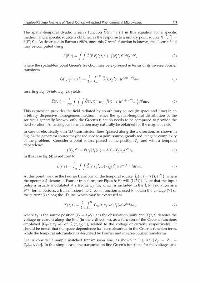
The spatial-temporal dyadic Green’s function G(�r,�r ′; t, t′) in this equation for a specificmedium and a specific source is obtained as the response to a unitary point source�J(�r ′, t′) =δ(�r ′; t′). As described in Barton (1989), once this Green’s function is known, the electric fieldmay be computed using
�E(�r, t) =∫ ∫
¯G(�r, �rg ′; t, t ′) ·�J(�rg ′, t′)d�rg ′dt′, (2)
where the spatial-temporal Green’s function may be expressed in terms of its inverse Fouriertransform
¯G(�r, �rg ′; t, t ′) = 12π
∫ +∞
−∞
˜G(�r, �rg ′; ω)ejω(t−t ′)dω. (3)
Inserting Eq. (3) into Eq. (2), yields
�E(�r, t) =1
2π
∫ ∫ ∫˜G(�r, �rg ′; ω) ·�J(�rg ′, t′)ejω(t−t ′)dr′gdt′dω. (4)
This expression provides the field radiated by an arbitrary source (in space and time) in anarbitrary dispersive homogenous medium. Since the spatial-temporal distribution of thesource is generally known, only the Green’s function needs to be computed to provide thefield solution. An analogous formulation may naturally be obtained for the magnetic field.
In case of electrically thin 1D transmission lines (placed along the z direction, as shown inFig. 5), the generator source may be reduced to a point source, greatly reducing the complexityof the problem. Consider a point source placed at the position �rg , and with a temporaldependence
�J(�rg, t′) =�κ(�rg)Ig(t′) = δ(�r−�rg)Ig(t′)ez. (5)
In this case Eq. (4) is reduced to
�E(�r, t) =1
2π
∫ ∫˜G(�r, �rg ′; ω) · Ig(t′)ezejω(t−t ′)dt′dω. (6)
At this point, we use the Fourier transform of the temporal source [ Ig(ω) = F{Ig(t′)}, wherethe operator F denotes a Fourier transform, see Pipes & Harvill (1971)]. Note that the inputpulse is usually modulated at a frequency ω0, which is included in the Ig(ω) notation as aejω0t term. Besides, a transmission-line Green’s function is used to obtain the voltage (V) orthe current (I) along the 1D line, which may be expressed as
X(z, t) =1
2π
∫ ∞
−∞GX(z, zg; ω) Ig(ω) ejωtdω, (7)
where zg is the source position (�rg = zgez), z is the observation point and X(z, t) denotes thevoltage or current along the line (in the z direction), as a function of the Green’s functionsemployed [GV(z, zg; ω) or GI(z, zg; ω), related to the voltage or current, respectively]. Itshould be noted that the space dependence has been absorbed in the Green’s function term,while the temporal information is described by Fourier and inverse-Fourier transforms.
Let us consider a simple matched transmission line, as shown in Fig. 5(a) [Zg = ZL =Z0(ω),∀ω]. In this simple case, the transmission line Green’s functions for the voltages and
31Impulse-Regime Analysis of Novel Optically-Inspired Phenomena at Microwaves
6 Will-be-set-by-IN-TECH
(a)
(b)
(c)
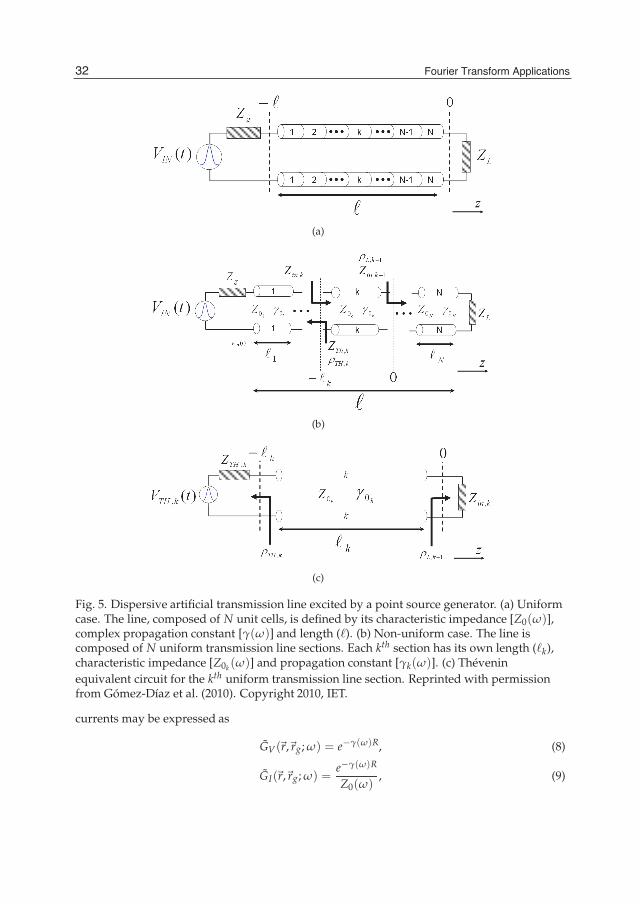
Fig. 5. Dispersive artificial transmission line excited by a point source generator. (a) Uniformcase. The line, composed of N unit cells, is defined by its characteristic impedance [Z0(ω)],complex propagation constant [γ(ω)] and length (�). (b) Non-uniform case. The line iscomposed of N uniform transmission line sections. Each kth section has its own length (�k),characteristic impedance [Z0k (ω)] and propagation constant [γk(ω)]. (c) Théveninequivalent circuit for the kth uniform transmission line section. Reprinted with permissionfrom Gómez-Díaz et al. (2010). Copyright 2010, IET.
currents may be expressed as
GV(�r,�rg; ω) = e−γ(ω)R, (8)
GI(�r,�rg; ω) =e−γ(ω)R
Z0(ω), (9)
32 Fourier Transform Applications

Impulse-Regime Analysis of Novel Optically-Inspired Phenomena at Microwaves 7
respectively, where γ(ω) is the complex propagation constant (or dispersion relation), Z0(ω)is the characteristic impedance, and R = |z− zg| is the distance between the observation pointz along the line and the source point zg (generator).
Using these expressions, the voltage or the current along the line can easily be foundwith Eq. (7). Note that this equation applies to any type of transmission line, includingmetamaterial CRLH lines, provided that the propagation constant [γ(ω)] is known.
Consider now the more general case of a nonuniform transmission line medium composed ofN uniform transmission line sections (or unit-cells), as shown in Fig. 5(b). The sections maybe different from each other and may be of different type. Therefore, reflections occur due tothe transition between two consecutive cells, and different propagation conditions appear ateach cell. The Green’s function along the kth uniform transmission line section (z ∈ [−�k, 0],possibly infinitesimal), including generator and load mismatches, reads
Gk(z, z′ = −�; ω) = A(ω)
[e−γk(ω)z+ ρl,k(ω)eγk(ω)z
], (10)
where [see Pozar (2005)]
A(ω) =VTh,k(ω)Zin,k(ω)
Zin,k(ω) + ZTh,k
e−γk(ω)�k
1 − ρl,k(ω)ρTh,k(ω)e−2γk(ω)�k, (11)
and
ρTh,k(ω) =ZTh,k(ω)− Z0k (ω)
ZTh,k(ω) + Z0k (ω), (12)
ρl,k(ω) =Zin,k+1(ω)− Z0k (ω)
Zin,k+1(ω) + Z0k (ω), (13)
which was obtained by equating the Green’s function evaluated at the input of the kth section,to the Thévenin’s voltage evaluated at the same section VTh,k [see Fig. 5(c)]. By repeatedlyapplying Eq. (10) from the load to the generator or vice-versa, the voltage as a function oftime may be computed at any point along the nonuniform transmission medium.
Finally, note that the use of periodic input signals is important to produce some periodicphenomena or devices, such as the Talbot effect introduced in Azaña & Muriel (2001) or theUWB resonator presented in Gómez-Díaz et al. (2009a), among many others. For this purpose,the theory previously introduced can easily be extended to consider this type of input signals.In this case, the input signal may be represented in the time domain by
I pg (t) =k=+∞
∑k=−∞
Ig(t− kT0), (14)
where T0 is the period rate. The voltage or current along the transmission line may then becomputed by inserting Eq. (14) in Eq. (7). Note that for many input pulses, such as modulatedGaussian pulses, the interchange between the integral and summation operations (related toEq. (7) and Eq. (14), respectively), allowed by the assumed linearity of the system, will furthercontribute to reduce the computational cost required by this technique.
33Impulse-Regime Analysis of Novel Optically-Inspired Phenomena at Microwaves
8 Will-be-set-by-IN-TECH
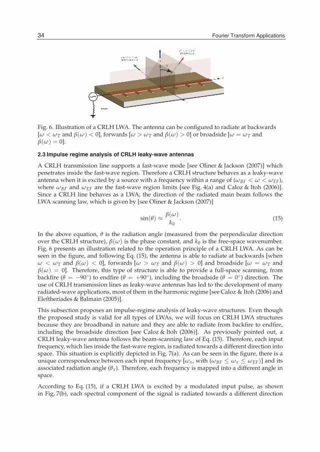
Fig. 6. Illustration of a CRLH LWA. The antenna can be configured to radiate at backwards[ω < ωT and β(ω) < 0], forwards [ω > ωT and β(ω) > 0] or broadside [ω = ωT andβ(ω) = 0].
2.3 Impulse regime analysis of CRLH leaky-wave antennas
A CRLH transmission line supports a fast-wave mode [see Oliner & Jackson (2007)] whichpenetrates inside the fast-wave region. Therefore a CRLH structure behaves as a leaky-waveantenna when it is excited by a source with a frequency within a range of (ωBF < ω < ωEF),where ωBF and ωEF are the fast-wave region limits [see Fig. 4(a) and Caloz & Itoh (2006)].Since a CRLH line behaves as a LWA, the direction of the radiated main beam follows theLWA scanning law, which is given by [see Oliner & Jackson (2007)]
sin(θ) ≈ β(ω)
k0. (15)
In the above equation, θ is the radiation angle (measured from the perpendicular directionover the CRLH structure), β(ω) is the phase constant, and k0 is the free-space wavenumber.Fig. 6 presents an illustration related to the operation principle of a CRLH LWA. As can beseen in the figure, and following Eq. (15), the antenna is able to radiate at backwards [whenω < ωT and β(ω) < 0], forwards [ω > ωT and β(ω) > 0] and broadside [ω = ωT andβ(ω) = 0]. Therefore, this type of structure is able to provide a full-space scanning, frombackfire (θ = −90◦) to endfire (θ = +90◦), including the broadside (θ = 0◦) direction. Theuse of CRLH transmission lines as leaky-wave antennas has led to the development of manyradiated-wave applications, most of them in the harmonic regime [see Caloz & Itoh (2006) andEleftheriades & Balmain (2005)].
This subsection proposes an impulse-regime analysis of leaky-wave structures. Even thoughthe proposed study is valid for all types of LWAs, we will focus on CRLH LWA structuresbecause they are broadband in nature and they are able to radiate from backfire to endfire,including the broadside direction [see Caloz & Itoh (2006)]. As previously pointed out, aCRLH leaky-wave antenna follows the beam-scanning law of Eq. (15). Therefore, each inputfrequency, which lies inside the fast-wave region, is radiated towards a different direction intospace. This situation is explicitly depicted in Fig. 7(a). As can be seen in the figure, there is aunique correspondence between each input frequency [ωx, with (ωBF ≤ ωx ≤ ωEF)] and itsassociated radiation angle (θx). Therefore, each frequency is mapped into a different angle inspace.
According to Eq. (15), if a CRLH LWA is excited by a modulated input pulse, as shownin Fig. 7(b), each spectral component of the signal is radiated towards a different direction
34 Fourier Transform Applications

Impulse-Regime Analysis of Novel Optically-Inspired Phenomena at Microwaves 9
(a) (b)
Fig. 7. Impulse-regime behavior of CRLH LWAs. (a) Frequency-space relationship of a CRLHLWA. The dispersion curve is graphically related to its corresponding beam scanning law. (b)Spectral decomposition of a pulse obtained by the frequency-space mapping property of aCRLH leaky-wave antenna. Reprinted with permission from Gupta, Abielmona & Caloz(2009). Copyright 2009, IEEE.
in space at any particular instant. Hence, the CRLH LWA performs an instantaneousspectral-to-spatial decomposition of the input pulse. This decomposition allows to discriminatethe various spectral components present in the input signal. In this sense, there is clearparallelism between LWAs (which usually operates at microwaves) and diffraction gratings[see Saleh & Teich (2007)], which usually operate at the optics regime and radiate each spatialinput frequency towards a different direction angle in space. The main advantage of CRLHLWA over diffraction gratings is its simple point feeding system as compared to the diffractiongratings, which require plane-wave illumination.
Let us consider a single 1D (or electrically thin) LWA, located along the z axis, as shown inFig. 8. It is important to clarify the notation employed to describe the situation under analysis.First, the line is defined by a characteristic impedance [Z0(ω)], a complex propagationconstant [γ(ω) = α(ω) + jβ(ω)], and a total length, �. Second, the generator which excitesthe transmission line is placed at the position�rg, with�rg = zgez. Third, any point along theline is denoted as�r ′, with�r ′ = z′ ez (note that zstart ≤ z′ ≤ zend, see Fig. 8). Besides, notethat shall study the far-field radiation of the transmission line towards an observation point P(denoted as�r, with�r = xex + yey+ zez). Therefore, any observation point P must be located inthe far-field region of the transmission line [see Balanis (2005)], fulfilling the far-field radiationcondition, which is given by
Rant =
√x2 + y2 +
(z− �
2
)2>
2�2
λ0. (16)
In this last equation, Rant is the distance between the observation point P (placed at�r) andthe transmission line, which can approximately be considered as a point source (placed at thecenter of the line) from a far-field point of view.
35Impulse-Regime Analysis of Novel Optically-Inspired Phenomena at Microwaves
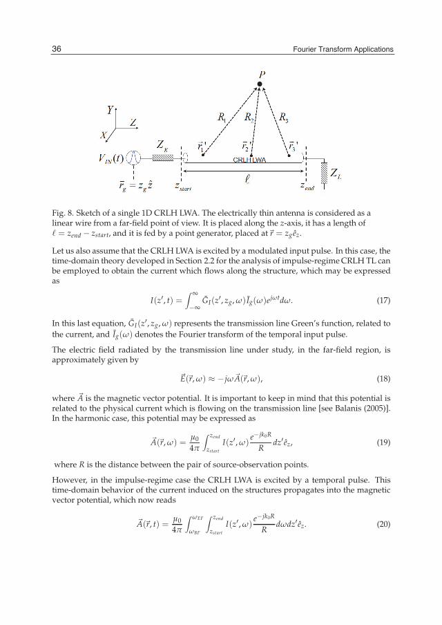
10 Will-be-set-by-IN-TECH
Fig. 8. Sketch of a single 1D CRLH LWA. The electrically thin antenna is considered as alinear wire from a far-field point of view. It is placed along the z-axis, it has a length of� = zend − zstart, and it is fed by a point generator, placed at�r = zgez.
Let us also assume that the CRLH LWA is excited by a modulated input pulse. In this case, thetime-domain theory developed in Section 2.2 for the analysis of impulse-regime CRLH TL canbe employed to obtain the current which flows along the structure, which may be expressedas
I(z′, t) =∫ ∞
−∞GI(z′, zg, ω) Ig(ω)ejωtdω. (17)
In this last equation, GI(z′, zg, ω) represents the transmission line Green’s function, related tothe current, and Ig(ω) denotes the Fourier transform of the temporal input pulse.
The electric field radiated by the transmission line under study, in the far-field region, isapproximately given by
�E(�r, ω) ≈ −jω�A(�r, ω), (18)
where �A is the magnetic vector potential. It is important to keep in mind that this potential isrelated to the physical current which is flowing on the transmission line [see Balanis (2005)].In the harmonic case, this potential may be expressed as
�A(�r, ω) =μ0
4π
∫ zend
zstartI(z′, ω)
e−jk0R
Rdz′ ez, (19)
where R is the distance between the pair of source-observation points.
However, in the impulse-regime case the CRLH LWA is excited by a temporal pulse. Thistime-domain behavior of the current induced on the structures propagates into the magneticvector potential, which now reads
�A(�r, t) =μ0
4π
∫ ωEF
ωBF
∫ zend
zstartI(z′, ω)
e−jk0R
Rdωdz′ ez. (20)
36 Fourier Transform Applications
Impulse-Regime Analysis of Novel Optically-Inspired Phenomena at Microwaves 11
It is important to remark that the frequency integration limits have been modified with respectto Eq. (7). Specifically, the frequency limits directly corresponds to the fast-wave region range(ωBF ≤ ω ≤ ωEF). This is because LWAs are only able to radiate spectral components whichlies inside this region. Outside of the fast-wave region, this type of structures behaves as atransmission lines as described in Caloz & Itoh (2006).
Finally, the time-domain electric field radiated by a CRLH LWA, under a far-field assumption,can easily be recovered using
�E(�r, t) =−jμ04π
∫ ωEF
ωBF
∫ zend
zstartω I(z′, ω)
e−jk0R
Rdωdz′ez. (21)
This expression provides the time-domain electric field radiation from a CRLH LWA excitedby a modulated input pulse, at any observation point placed in the far-field region. The mainfeatures of this closed-form formulation are:
• All CRLH LWA radiation features at far-field are taken into account by using a time-domaincurrent along the structure. This current is closely related to the complex propagationconstant of the structure.
• Physical insight into the antenna radiation properties. The Green’s function and thecurrent flowing along the structure, related to the CRLH structure, completely define theantenna behavior. These parameters are obtained in closed-form.
• Extremely fast computation, because most expressions are simple and well-behavedintegrals (and some of them are analytical for specific input pulses).
• Capability to deal with any type of input pulse, providing a continuous temporal outputwith unconditional stability.
The proposed approach can characterize complex radiated-wave UWB phenomena anddevices. Specifically, this formulation will be employed in the next section to model severalsystems, such as a real-time spectrum analyzer (RTSA) or a frequency-resolved electricalgating system (FREG). It will be shown that the proposed formulation is able to completelycharacterize these systems with high efficiency and accuracy .
3. Optically-inspired phenomena at microwaves
3.1 Introduction
This section explores the impulse-regime phenomenology of CRLH structures and thesubsequent theoretical and practical demonstration of several novel optically-inspiredphenomena and applications at microwaves, in both, the guided and the radiative regime. Thetime-domain Green’s function approach introduced in Section 2 has opened the door to a veryfast, but still accurate, analysis of these novel microwave phenomena and applications, mostof them transported from optics, exploiting either the group velocity or the group velocitydispersion parameters of CRLH TL. The study can be divided into two main groups, relatedto the guided-wave or radiative-wave natures of the proposed phenomena and applications.
The analogy between these phenomena at microwave and their corresponding counterpart at optics [seeSaleh & Teich (2007)] is deduced from the dispersive properties of CRLH structures. Specifically, inthe guided mode there is a clear parallelism between the dispersive behavior of a CRLH lineand an optical component (such as an optical fiber), which is inherently dispersive. Therefore,
37Impulse-Regime Analysis of Novel Optically-Inspired Phenomena at Microwaves

12 Will-be-set-by-IN-TECH
optical phenomena [such as the well-known temporal Talbot effect] can be reproduced atmicrowaves. In the radiative mode, the beam scanning law of the CRLH LWA is analogto a diffraction grating, where different spectral components are radiated (or diffracted) atdifferent angles causing spatial dispersion. This may be exploited to develop spectrogramanalyzers, capable to fully characterize both, in time and frequency, any unknown inputsignal.
3.2 Guided-regime
This subsection presents a study on the phenomenology of pulse propagation along CRLHtransmission lines. As previously stated, the CRLH TL represents a general transmissionmedium, which is highly dispersive, especially in the left-handed frequency range. Next,the temporal Talbot effect [see Azaña & Muriel (1999)] is introduced, theoretically describedand numerically confirmed for the case of CRLH media.
3.2.1 Pulse propagation along CRLH structures
The main goal of this subsection is to experimentally validate the theory presented inSection 2. For this purpose, the propagation of a modulated pulse along a CRLH TL is studied.The tunability of the pulse delay as a function of the modulation frequency is demonstratedby measuring the temporal delay from different modulated pulses, leading to a tunable delaysystem [see Abielmona et al. (2007)]. Then, the dispersive features of the CRLH TL are furtherdemonstrated monitoring the effects of pulse propagation along a matched and mismatchedline, in a cell-by-cell fashion.
First, we consider a CRLH transmission line composed of 30 unit cells and with the circuitparameters CR = 1.8 pF, CL = 0.9 pF, LR = 3.8 nH and LL = 1.9 nH (transition frequencyf0 = 2.55 GHz), excited by a modulated Gaussian pulse [σ = 3.0 ns, following the notationintroduced in Saleh & Teich (2007)]. Fig. 9 shows the time-delayed waveforms obtained bythe proposed theory for different carrier frequencies, and by experiments using a real-timeoscilloscope (Agilent Infiniium DS0871204B). Excellent agreement is observed between theoryand experiments. The group delay response is an important parameter in dispersive systemsfor analog signal processing applications. This parameter may be computed either in the timedomain by determining the time differences between the maxima of the input and outputpulses, or in the frequency domain by taking the derivative of the unwrapped phase ofthe transmission scattering parameter S21. Fig. 10 shows the group delay along the sameCRLH line and for the same pulse as in Fig. 9, computed by the discussed theory usingthe first approach, and validated by experiment using both approaches. Again, very goodagreement is observed between theory and experiment. The small discrepancies betweenthe two measured results may be explained by the tolerance in the localization of the pulsemaxima. As it may be seen from these results and was originally presented in Abielmona et al.(2007), the CRLH transmission line acts as an impulse tunable delay system.
To better visualize the dispersion of a pulse along a CRLH dispersive medium, consider nowa CRLH transmission line twice as long as before (60 unit cells), but with the same parameters.To completely validate the discussed theory, this time the line is excited by a modulated squarepulse [ f0 = 2.05 GHz, T = 2.2 ns, following the notation of Saleh & Teich (2007)]. An ABCDmatrix approach, described in Caloz & Itoh (2006), is employed to compute the propagationconstant of the line, taking into account the finite number of unit cells in the experiment. Theposition-time trajectory of the pulse is presented in Fig. 11. Fig. 11(a) shows the computed
38 Fourier Transform Applications

Impulse-Regime Analysis of Novel Optically-Inspired Phenomena at Microwaves 13
Fig. 9. Time-delayed Gaussian waveforms at the input/output of a CRLH transmission linefor different carrier frequencies, obtained with the method proposed in Section 2.2.Measurement results are also shown for validation. The manufactured CRLH transmissionline is shown in the inset. Reprinted with permission from Gómez-Díaz et al. (2009b).Copyright 2009, IEEE.
1.8 2 2.2 2.4 2.6 2.8 3 3.2 3.44
5
6
7
8
9
10
11
Frequency [GHz]
Del
ay [n
sec]
Proposed theory, from pulse maxima locations in timeMeasured, from pulse maxima locations on oscilloscopeFrom derivation of measured unwrapped phase of S
21(ω)
4,68
9.12
Fig. 10. Time delay versus modulation frequency, using the time difference between themaxima of the input and output pulses along the same CRLH line as in Fig. 9. Measured datausing both, the same procedure as before and unwrapping the phase of S21(ω), are alsoshown for validation. The delays obtained in Fig. 9 for fc = 3.2 GHz and fc = 1.9 GHz,which are 4.68 and 9.12 ns, correspond to the two highlighted points. Reprinted withpermission from Gómez-Díaz et al. (2009b). Copyright 2009, IEEE.
results, from which two observations may be made: i) at the end of the line, the temporalwidth of the pulse has increased by a factor of 5 (at 50% of the magnitude), ii) the edges of thesquare envelope have been rounded off by the band-pass filtering response of the CRLH line.The small ripples near the end of the structure are explained by the Gibbs effect on the inputpulse due to the finite computational interval and resolution. Fig. 11(b) shows the measuredresult using a high-impedance probe connected to the oscilloscope. The abrupt decrease ofthe voltage magnitude after the 30th cell is due to the fact that the 60-cell experimental line is
39Impulse-Regime Analysis of Novel Optically-Inspired Phenomena at Microwaves

14 Will-be-set-by-IN-TECH
(a) (b)Fig. 11. Propagation of a modulated square pulse ( f0 = 2.05 GHz, T = 2.2 ns) along amatched CRLH transmission line. The line includes 60 unit cells of length p = 2.0 cm and thecircuital parameters are CR = 1.8 pF, CL = 0.9 pf, LR = 3.8 nH and LL = 1.9 nH. (a)Simulation. (b) Measurement. Reprinted with permission from Gómez-Díaz et al. (2009b).Copyright 2009, IEEE.
(a) (b)Fig. 12. Propagation of a modulated square pulse ( f0 = 2.05 GHz, T = 2.2 ns) along anopen-ended CRLH transmission line. The line is identical to that of Fig. 11 except that itincludes only 30 unit cells. (a) Simulation. (b) Measurement. Reprinted with permission fromGómez-Díaz et al. (2009b). Copyright 2009, IEEE.
in fact constituted of two cascaded 30-cell lines with a small loss in the interconnection. Theagreement with theory is reasonable, considering the tolerances of the measurement setup.Finally, let us investigate the effects of the reflection of a pulse at a discontinuity of a CRLHtransmission line. For this purpose, the line is open-ended and it is excited by the samemodulated square pulse as in the previous case. The propagation and the reflection of thepulse as a function of space and time is presented in Fig. 12. Again, good agreement isobserved between the theory [Fig. 12(a)] and the experiment [Fig. 12(b)]. It is worth noticingthat an interesting interference pattern, between propagating and reflected pulses, occurs nearthe discontinuity.
3.2.2 Temporal Talbot effect
The Talbot effect is a periodic constructive interference pattern produced by a dispersivetransmission medium with second-order dispersion for a periodic input signal. It was firstreported by H. F. Talbot in 1836 for the case of a source with periodic spatial variation[see Talbot (1836)]. The temporal counterpart of this effect [see Azaña & Muriel (1999) orAzaña & Muriel (2001)] occurs when a time-periodic signal is propagating along the samekind of medium. An input pulse train with temporal period T0 and pulse width ΔT is
40 Fourier Transform Applications
Impulse-Regime Analysis of Novel Optically-Inspired Phenomena at Microwaves 15
replicated at the position nzT (n ∈ N), where zT is called the Talbot distance (or self-imagingdistance). Also, an increased repetition rate of m pulses per T0 is obtained at the fractionaldistances z f = (s/m)zT (where s,m ∈ N), provided that (s/m) is an irreducible fraction,and under the condition that: m < T0/ΔT [see Azaña & Muriel (2001)]. The temporalTalbot effect has been employed mainly in the optical regime, for applications such as thegeneration of signals with ultrahigh repetition rate (THz) from slower ranges (GHz), as shownin Azaña & Muriel (2001), or pulse compression, as presented in detail in Berger et al. (2004).
At microwaves, this phenomenon is more difficult to reproduce because it is difficult to obtaina second-order dispersive medium at this frequency region. However, the recent introductionof CRLH TLs [see Caloz & Itoh (2006)], which provides a dispersive broadband behavior, maylead to novel scenarios where the temporal Talbot effect and their subsequent applicationscan be reproduced. This section provides a theoretical demonstration of the temporal Talboteffect in CRLH media, including a full-wave validation of the phenomena at microwaves.Furthermore, the conditions for the phenomena existence in CRLH media are stated, inconnection with potential device applications.
Intuitively, the temporal Talbot effect occurs when a periodic pulse signal is transmittedthrough a second order dispersion medium where the neighboring pulses interfere as a resultof dispersion so as to produce new temporal components. For the analysis, let us considera single modulated pulse, denoted by Ψ(t) = Ψ0(t)ejω0t, where Ψ0(t) is a slowly varyingenvelope. The periodic signal is then represented in the time domain, at the position z = 0, as
A(z = 0, t) =n=+∞
∑n=−∞
Ψ(t− nT0), (22)
where T0 is the repetition rate of the signal. In the spectral domain, the periodic signalbecomes discrete, and it may be expressed as
A(z = 0, ω) = ωr
n=+∞
∑n=−∞
Ψ(ω = nωr)δ(ω − nωr), (23)
where ωr = 2π/T0 is the spectral repetition frequency.
On the other hand, the transfer function of a lossless CRLH TL is given by
H(z, ω) = e−jβ(ω)z, (24)
where β(ω) is the CRLH TL propagation constant. This propagation constant, around theCRLH TL transition frequency, may be approximated as
β(ω) =ω
ω′R− ω′
Lω
, (25)
where ω′R = p/
√LRCR and ω′
L = 1/√p2LLCL, as described in Caloz & Itoh (2006). In the
right handed side of Eq. (25), the first term provides a simple time delay (or linear frequencyphase), whereas the second order term is responsible for the line dispersion. Eq. (25) can befurther expanded, employing Taylor series, around a modulation frequency (ω0) as
β(ω) = β0 + β1(ω − ω0) +12
β2(ω − ω0)2 +O(ω3), (26)
41Impulse-Regime Analysis of Novel Optically-Inspired Phenomena at Microwaves
16 Will-be-set-by-IN-TECH
where the termO(ω3) is related to the order of the error committed in the approximation, andthe term βn is defined as
βn =
[βn(ω)
∂ωn
]∣∣∣∣ω=ω0
. (27)
Note that Eq. (26) is only valid for the case of narrowband pulses (centered at the frequencyω0 and with bandwidth Δω).Employing Eq. (26), the transfer function of the CRLH TL
[H(ω′) = H(ω = ω0 + ω′) , where
a change of variable has been introduced from ω to ω′ ] takes the form
H(z, ω′) = exp{−j
[β0 + β1ω′ + 1
2β2ω′2
]z}
. (28)
In order to derive the Talbot distance, only the third expansion term of the exponential isconsidered. This is because the first two terms do not provide any information related to theTalbot distance [which is only due to second order dispersion, see Azaña & Muriel (2001)].Specifically, the first term is related to the modulation frequency of the pulse and does notcarry any information about the envelope, and the second term represent the group delay (orretarded frame) of the signal.
Using Eq. (23) and Eq. (28), the spectrum of the signal at the distance z can be written as
A(z, ω′) =ωr
n=+∞
∑n=−∞
exp{−j β2ω′2z
2
}Ψ(nωr)δ(ω
′ − nωr) = (29)
ωr
n=+∞
∑n=−∞
exp
{−j β2z
2
(2πnT0
)2}
Ψ(nωr)δ(ω′ − nωr).
Note that the appearance of ω′ squared term in this equation is due to the quadratic phasefactor in the spectral response of the CRLH TL dispersive medium.
Eq. (29) reveals that the Talbot effect [ i.e., Az(z, ω) = A(z = 0, ω) ] occurs under the condition
β2z2
(2πnT0
)2= πp, (30)
where p ∈ N. The case of the first integer Talbot distance (p = 1) is given by
zT =T2
02π|β2| =
T20 ω3
0
4πω′2L
, (31)
where the identity β2 = −2ω′2L /ω3
0 [see Eq. (27)] has been employed.
As demonstrated in Azaña & Muriel (2001), the Talbot distance can also be obtained atfractionary distances given by z f = (s/m)zT, where s and m are irreducible integers. Atthis fractionary distance, the periodic input signal is also self-imaged but with an increaserepetition rate by a factor of m. This phenomenon corresponds to the fractionary Talbot effect[see Azaña & Muriel (2001)]. It is important to note that in the case of a CRLH TL, the Talbotdistance can be tuned externally by modifying the parameters T0 and ω0, without changingthe intrinsic parameters of the line.
42 Fourier Transform Applications

Impulse-Regime Analysis of Novel Optically-Inspired Phenomena at Microwaves 17
(a)
210 220 230 240 2500
0.2
0.4
0.6
0.8
1
1.2
Nor
mal
ized
vol
tage
Time [nsec]
InputOutput from TD−GFOutput from ADS
(b)
210 220 230 240 2500
0.2
0.4
0.6
0.8
1
1.2
Nor
mal
ized
vol
tage
Time [nsec]
InputOutput from TD−GFOutput from ADS
(c)
210 220 230 240 2500
0.2
0.4
0.6
0.8
1
1.2
Nor
mal
ized
vol
tage
Time [nsec]
InputOutput from TD−GFOutput from ADS
(d)
Fig. 13. Talbot repetition rate multiplication effect. a) CRLH TL with length corresponding tothe basic Talbot distance zT. b) Reconstruction of the original pulse train at the Talbotdistance zT . c) Repetition rate doubling at the distance zT/2. d) Repetition rate tripling at thedistance zT/3. Results obtained from the proposed approach, and validated using thecommercial software ADS©. Reprinted with permission from Gómez-Díaz et al. (2009b).Copyright 2009, IEEE.
After theoretically deriving the Talbot distance related to CRLH TLs, the phenomena willbe verified using the numerical technique proposed in Section 2.2 and commercial full-wavesimulations. Consider a balanced lossless CRLH transmission line with circuital parametersCR = CL = 1.0 pF and LR = LL = 2.5 nH. A modulated train of Gaussian pulses, withtemporal width of σ = 0.75 ns and period rate of T0 = 8 ns is used to excite the line shownin Fig. 13(a). Fig. 13(b) presents the input pulse train and the output pulse train at the Talbotdistance zT . The reconstruction of the initial train of pulses is confirmed, although a smalldisagreement, due to higher order terms (greater than 2) of the CRLH dispersion relation,is observed between two consecutive pulses. Fig. 13(c) and Fig. 13(d) show the input andoutput voltages at the fractional Talbot distances of zT/2 and zT/3, respectively. The effectof pulse multiplication is thus clearly confirmed, while the distortion is smaller because lesshigher-order dispersion effects occur over a shorter distance of propagation.
The practical implementation of Talbot devices based on CRLH transmission lines dependson the technology employed. For instance, with the CRLH parameters used in Fig. 13, amicrostrip implementation with a typical unit cell size of 1 cm would lead to a Talbot distancezT of around 17 meters. This is unpractical, specially due to the losses. However, using
43Impulse-Regime Analysis of Novel Optically-Inspired Phenomena at Microwaves
18 Will-be-set-by-IN-TECH
multilayer technology [see Horii et al. (2005)], this distance may be dramatically reduced tosizes in the order of several centimeters, while even lower sizes apply for pulse rate repetitionmultiplication. This decrease in length also decreases the total amount of losses, allowingthe Talbot effect to be applied in practical situations, such as the generation of signals withultrahigh repetition rate or pulse compression [see Berger et al. (2004)].
3.3 Radiative-regime
The full-space scanning capabilities of CRLH LWAs are exploited in this Section toachieve the spectral-spatial decomposition of an input broadband signal. This propertyis then applied to the development of a real-time spectrum analyzer [RTSA, seeGupta, Abielmona & Caloz (2009)] and a frequency resolved electrical gating system[FREG, see Gupta, Gómez-Díaz & Caloz (2009)], which are UWB applications able to fullycharacterize, in both time and frequency, an unknown signal. These systems are fully modeledby the technique presented in Section 2.3, which constitutes an ideal tool to provide not onlya fast numerical system characterization, but a deep physical insight into the electromagneticproperties of the devices.
3.3.1 Real time spectrogram analyzer (RTSA)
A real time spectrogram analyzer (RTSA) is a device able to provide a joint time-frequencyrepresentation of an unknown input signal. This device is specially useful in modern UWBsystems, as described in Ghavami et al. (2007), where ultra-fast transient signals are involved.The common output of a RTSA system is an spectrogram [see Cohen (1989)], which is a 2-D plotof a signal where the energy distribution is related to an image in a time-frequency plane. Thejoint time-frequency representation provides information related to the temporal evolution ofeach spectral component, and the exact amplitude and location in time of each frequency. It isimportant to mention that spectrograms suffer from the fundamental "uncertainty principle"limitation, which states
ΔtΔ f ≥ 12
, (32)
where Δ f is the bandwidth of the gated signal and Δt is the gate duration. This implies aninherent trade off between time and frequency resolution for all spectrograms.
There are two main approaches to obtain the spectrogram of an unknown input test signalat microwave frequencies. The first and more usual technique is based on the use of digitalcomponents, which performs the short-time Fourier transform (STFT) [see Oppenheim (1996)]of the unknown input signal. However, the use of this approach at microwaves has theimportant drawback of requiring fast processors and large memories, which limits its useto input signals of just a few hundreds megahertz and temporal resolutions of only a fewmicroseconds. The second option, purely analog, is based on the use of a bank of filters, asdescribed in Amin & Feng (1995). The main disadvantage of this approach is that it requires avery large number of channels and extremely narrow-band filters, which is specially difficultto achieve at high frequencies. Consequently, this option is very complex and expensive.
In this context, a novel RTSA based on the spectral-spatial decomposition of CRLH LWAs wasproposed in Gupta, Abielmona & Caloz (2009). In this approach, the CRLH LWA provides ananalog implementation of the STFT, in a similar way as it has been implemented in the opticalregime. A schematic of the CRLH LWA RTSA system is shown in Fig. 14. The description ofthe system behavior is as follows. First, the spectral-spatial decomposition of the CRLH LWA
44 Fourier Transform Applications
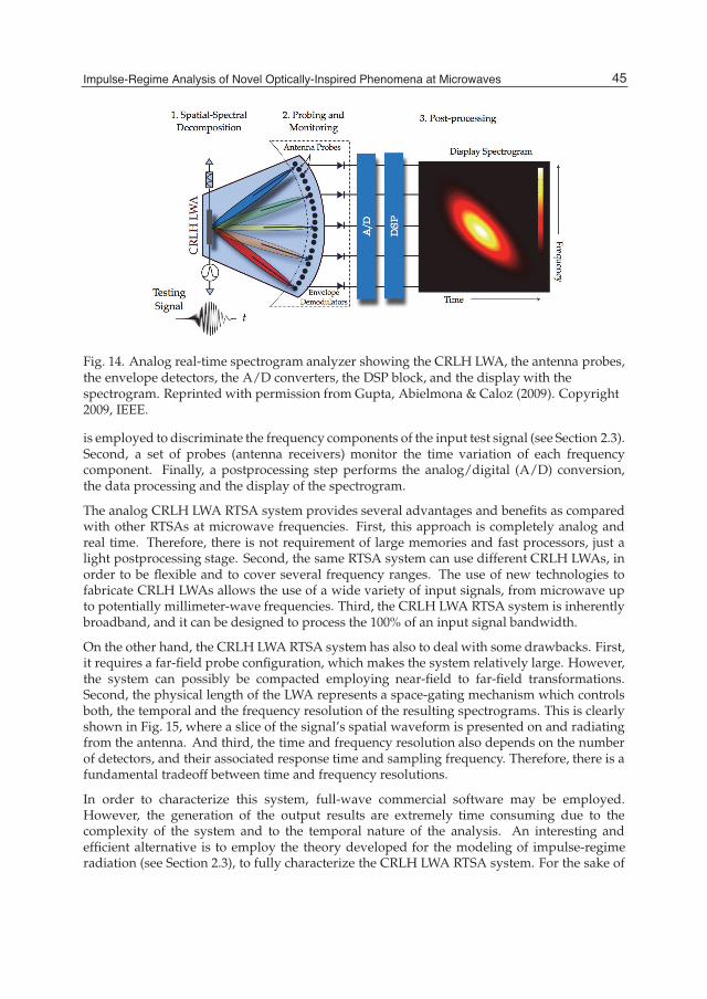
Impulse-Regime Analysis of Novel Optically-Inspired Phenomena at Microwaves 19
Fig. 14. Analog real-time spectrogram analyzer showing the CRLH LWA, the antenna probes,the envelope detectors, the A/D converters, the DSP block, and the display with thespectrogram. Reprinted with permission from Gupta, Abielmona & Caloz (2009). Copyright2009, IEEE.
is employed to discriminate the frequency components of the input test signal (see Section 2.3).Second, a set of probes (antenna receivers) monitor the time variation of each frequencycomponent. Finally, a postprocessing step performs the analog/digital (A/D) conversion,the data processing and the display of the spectrogram.
The analog CRLH LWA RTSA system provides several advantages and benefits as comparedwith other RTSAs at microwave frequencies. First, this approach is completely analog andreal time. Therefore, there is not requirement of large memories and fast processors, just alight postprocessing stage. Second, the same RTSA system can use different CRLH LWAs, inorder to be flexible and to cover several frequency ranges. The use of new technologies tofabricate CRLH LWAs allows the use of a wide variety of input signals, from microwave upto potentially millimeter-wave frequencies. Third, the CRLH LWA RTSA system is inherentlybroadband, and it can be designed to process the 100% of an input signal bandwidth.
On the other hand, the CRLH LWA RTSA system has also to deal with some drawbacks. First,it requires a far-field probe configuration, which makes the system relatively large. However,the system can possibly be compacted employing near-field to far-field transformations.Second, the physical length of the LWA represents a space-gating mechanism which controlsboth, the temporal and the frequency resolution of the resulting spectrograms. This is clearlyshown in Fig. 15, where a slice of the signal’s spatial waveform is presented on and radiatingfrom the antenna. And third, the time and frequency resolution also depends on the numberof detectors, and their associated response time and sampling frequency. Therefore, there is afundamental tradeoff between time and frequency resolutions.
In order to characterize this system, full-wave commercial software may be employed.However, the generation of the output results are extremely time consuming due to thecomplexity of the system and to the temporal nature of the analysis. An interesting andefficient alternative is to employ the theory developed for the modeling of impulse-regimeradiation (see Section 2.3), to fully characterize the CRLH LWA RTSA system. For the sake of
45Impulse-Regime Analysis of Novel Optically-Inspired Phenomena at Microwaves

20 Will-be-set-by-IN-TECH
Fig. 15. Impact of the LWA size � on the time-frequency resolution of the spectrogramsgenerated by the an analog CRLH LWA RTSA.
validation, let us consider a complete RTSA system based on a CRLH LWA which is composedof 32 unit cells of length p = 1.0 cm, with circuital parameters of CR = CL = 1.0 pF andLR = LL = 2.5 nH. In order to complete the analog RTSA system, a total of number of 181observation probes are placed in a semi-circular configuration, following the configuration ofFig. 14. The first step to model the RTSA is to perform the calibration of the system. This isnecessary to compensate for the different power levels received at each probe [as describedin Gómez-Díaz et al. (2010)], due to the directivity variation with frequency of this type ofantennas. For the calibration, a narrow-band signal is modulated to the different fast-wavefrequencies [following Eq. (15) (scanning law)] and subsequently radiated by the LWA. Then,the maximum power received at each probe is stored, obtaining a normalization rule for thisparticular system configuration. In our example, the calibration data is shown in Fig. 16(a).After the RTSA system has been calibrated, it can be efficiently used to obtain spectrogramsof an unknown input signal. For the method validation, the actual temporal and frequencyinformation of an input test signal, previously known, is employed.
Let us consider now that the CRLH LWA is fed by a signal composed of three modulatedGaussian pulses. The first pulse has a positive-chirp modulation (which means that themodulation frequency is increasing with time), and the third pulse has a negative-chirpmodulation. The spectrogram obtained with the proposed method, after calibration, isdepicted in Fig. 16(b), including an additional graph showing the analytical temporalrepresentation of the signal. As can be observed in the figure, the spectrogram follows thesignal variations in time (the three pulses are clearly observable) and also, simultaneously,in frequency. It is especially interesting to observe the transition between two consecutivepulses, where frequencies corresponding to different pulses appear at the same instant.
The method proposed here is able to perform a quick (about 30 seconds) and accuratemodeling of the RTSA system, with deep insight into the CRLH LWA time-radiationproperties, and avoiding the extremely time-consuming analysis required in full-wavesimulations (usually between 8 − 12 hours). Therefore, it provides a fast tool to configurean RTSA system and to determine a priory the range of input signals which can accurately becharacterized for a given CRLH LWA.
46 Fourier Transform Applications

Impulse-Regime Analysis of Novel Optically-Inspired Phenomena at Microwaves 21
−90 −60 −30 0 30 60 900
10
20
30
40
50
60
70
Angle [º]
Max
imum
ele
ctric
fiel
d [V
/m]
(a) (b)Fig. 16. Results obtained from an RTSA system based on a CRLH LWA composed of 32 unitcells of length p = 1.0 cm, with circuital parameters of CR = CL = 1.0pF andLR = LL = 2.5nH. (a) Maximum electric field obtained at the different positions of theprobes, used for the calibration of the RTSA system. (b) Normalized spectrogram of a threechirp-modulated Gaussian pulses signal, with chirp parameters C = −[10, 0, 10], modulationfrequency f0 = 3.19 GHz and temporal width σ = 1.0 ns, computed with the proposedtechnique. The inset shows the analytical time response of the signal. Reprinted withpermission from Gómez-Díaz et al. (2010). Copyright 2010, IET.
Finally, experimental results from a RTSA prototype are included for a complete systemvalidation and to confirm the accuracy of the proposed modeling technique. For thispurpose, a CRLH LWA fabricated in microstrip technology and composed of 14 -0.8 cm-long unit cells, with circuital parameters CR = 1.29 pF, CL = 0.602 pF, LR = 3.0 nH andLL = 1.4 nH, is employed. A photo of the fabricated antenna is depicted in Fig. 17(a),whereas a comparison of the measured and simulated scattering parameters is shown inFig. 17(b). Furthermore, Fig. 17(c) presents a simulation-measurements comparison of theantenna dispersion relationship. As can be observed, the CRLH LWA presents its transitionfrequency at 3.745 GHz. The antenna fast-wave frequency region starts at about 3.1 GHz(related to backfire radiation), and it is extended until 4.7 GHz (related to endfire radiation).Note that several resonances occur within the fast-wave frequency region (close to endfire),degrading the antenna performance. These resonances are due to internal resonances of theinterdigital capacitors employed in the antenna prototype, and they are not considered in thecircuital model of the LWA.
In order to measure the spectrogram of the test signals, a single receiver was used and rotatedaround the circular far-field trajectory of the system (specifically, between θ = −80◦ and θ =80◦ with increments of 5◦). The RTSA system is calibrated employing a linear frequency ramp.After calibration, the CRLH LWA is excited by a modulated Gaussian pulse, with FWHMof 3.5 ns. Fig. 18 presents a comparison between simulations (obtained by the proposedtime-domain Green’s function approach) and measurements, as a function of the pulsemodulation frequency. It can be observed that a very good agreement is achieved in all cases.First, the pulse modulation frequency is set to 3.3 GHz, which corresponds to backwardsradiation. This is clearly shown in the spectrograms of Fig. 18(a) and Fig. 18(b). Then the
47Impulse-Regime Analysis of Novel Optically-Inspired Phenomena at Microwaves

22 Will-be-set-by-IN-TECH
(a)
1 2 3 4 5−80
−70
−60
−50
−40
−30
−20
−10
0
Frequency [GHz]
Sca
tterin
g P
aram
eter
s [d
B]
S11 MeasuredS21 MeasuredS11 CircuitalS21 Circuital
Fast−wave region
Transition Frequency
(b)
−400 −300 −200 −100 0 100 2001
1.5
2
2.5
3
3.5
4
4.5
5
β [rad/m]
Fre
quen
cy [G
Hz]
Circuital ModelMeasurementFree−Space
(c)Fig. 17. 1D CRLH LW antenna composed by 14 -0.8 cm- long cells, with circuital parametersCR = 1.29 pF, CL = 0.602 pF, LR = 3.0 nH and LL = 1.4 nH. a) Photo of a microstrip CRLHLWA prototype. b) Scattering parameters. c) Dispersion relation. Reprinted with permissionfrom Gómez-Díaz et al. (2009c). Copyright 2009, American Institute of Physics.
modulation frequency is set to the CRLH LWA transition frequency, which corresponds tobroadside radiation. As expected, the obtained spectrograms [see Fig. 18(c) and Fig. 18(d)]confirm the change in frequency. Finally, pulse modulation frequency is set to 4.2 GHz, whichcorresponds to a forward direction. Again the spectrograms show the changes in the pulsefrequency, experimentally verifying the RTSA system and confirming the usefulness of theproposed theoretical approach to model this type of analog systems.
3.3.2 Frequency resolved electrical gating system (FREG)
Analog CRLH LWA RTSAs generate the spectrogram of an unknown input signal in real-time,using the spectral-spatial decomposition property of the leaky-wave antenna, with minimalrequirements on computational resources. This system provides important benefits over anydigital RTSAs at microwave frequencies. However, as explained in the previous section, thetime and frequency resolution of the generated spectrograms directly depends on the physicallength of the CRLH LWA, which is fixed in a given system. Therefore, a particular antennacan only handle a limited range of input signals, which must fulfil specific time and frequencyconstrains. This imposes an important limitation to the CRLH LWA RTSA systems.
This section proposes a novel analog approach to obtain spectrograms, where the hardwaredependence is suppressed, at the cost of the requirement of periodicity of the input signals.This approach is inspired from a similar system known in optics as frequency resolved opticalgating (FROG) [see Trebino (2002)], where a self-gating principle is applied to provide closeto ideal spectrograms for arbitrary test signals. Here, we propose a microwave counterpart of
48 Fourier Transform Applications

Impulse-Regime Analysis of Novel Optically-Inspired Phenomena at Microwaves 23
(a) (b)
(c) (d)
(e) (f)
Fig. 18. Spectrograms obtained by the proposed RTSA model (figures on the left) and byexperiments (figures on the right), employing the CRLH LWA of Fig. 17. A modulatedGaussian pulse with FWHM = 3.5 ns feeds the antenna. The pulse modulation frequency isset to 3.3, 3.745 and 4.2 GHz, corresponding to backward [(a) and (b)], broadside [(c) and (d)]and forward [(e) and (f)] radiation, respectively.
49Impulse-Regime Analysis of Novel Optically-Inspired Phenomena at Microwaves
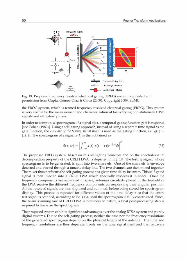
24 Will-be-set-by-IN-TECH
Fig. 19. Proposed frequency resolved electrical gating (FREG) system. Reprinted withpermission from Gupta, Gómez-Díaz & Caloz (2009). Copyright 2009, EuMC.
the FROG system, which is termed frequency resolved electrical gating (FREG). This systemis very useful for the measurement and characterization of fast-varying non-stationary UWBsignals and ultrashort pulses.
In order to compute a spectrogram of a signal x(t), a temporal gating function g(t) is required[see Cohen (1989)]. Using a self-gating approach, instead of using a separate time signal as thegate function, the envelope of the testing signal itself is used as the gating function, i.e. g(t) =|x(t)|. The spectrogram of a signal x(t) is then obtained as
S(τ, ω) =
∣∣∣∣∫ ∞
−∞x(t)|x(t− τ)|e−jωtdt
∣∣∣∣2 . (33)
The proposed FREG system, based on this self-gating principle and on the spectral-spatialdecomposition property of the CRLH LWA, is depicted in Fig. 19. The testing signal, whosespectrogram is to be generated, is split into two channels. One of the channels is envelopedetected and passed through a tunable delay line. The two channels are then mixed together.The mixer thus performs the self-gating process at a given time delay instant τ. This self-gatedsignal is then injected into a CRLH LWA which spectrally resolves it in space. Once thefrequency components are separated in space, antennas circularly placed in the far-field ofthe LWA receive the different frequency components corresponding their angular position.All the received signals are then digitized and summed, before being stored for spectrogramdisplay. This process is repeated for different values of the time delay τ so that the entiretest signal is scanned, according to Eq. (33), until the spectrogram is fully constructed. Since,the beam scanning law of CRLH LWA is nonlinear in nature, a final post-processing step isrequired to linearize the spectrogram.
The proposed system exhibits significant advantages over the analog RTSA system and purelydigital systems. Due to the self-gating process, neither the time nor the frequency resolutionsof the generated spectrogram depend on the physical length of the antenna. The time andfrequency resolutions are thus dependent only on the time signal itself and the hardware
50 Fourier Transform Applications

Impulse-Regime Analysis of Novel Optically-Inspired Phenomena at Microwaves 25
Fig. 20. Simulated spectrograms. a) Down-chirped gaussian pulse (C1 = −10, C2 = 0,f0 = 4 GHz). b) Non-chirped super-gaussian pulse (C1 = C2 = 0, f0 = 3 GHz). c)Up-chirped gaussian pulse (C1 = +10, C2 = 0, f0 = 4 GHz). d) Cubically chirped gaussianpulse (C1 = 0, C2 = 0.25 × 1028). All pulse have a FWHM duration of 1 ns with a initial pulseoffset of t0 = 6.5 ns, and are described using Eq. (34). Reprinted with permission fromGupta, Gómez-Díaz & Caloz (2009). Copyright 2009, EuMC.
dependence spectrogram is suppressed. The LWA simply plays a role of spectral decomposerwhich, when longer (higher directivity), provides better separation of frequencies in space.
The choice of the gate duration is an important parameter to achieve an optimaltime-frequency resolution in the spectrogram. An optimal gate duration for pulses withdominating phase variations is given by Tg ≈ 1/
√2|φ′′(t)|, where φ′′(t) is the second
time derivative of phase [see Cohen (1989)]. This duration permits the resolution of thefastest phase variations. For general pulse measurement, a gate duration as short as thetesting signal itself or slightly shorter is thus desirable. Since the FREG system is based onself-gating, the gate duration is close to optimal and the corresponding spectrograms are ideal,as demonstrated in Trebino (2002).
Moreover, the proposed system being analog in nature, neither require fast processors norhuge memory buffers, which avoid placing a heavy computational burden on the system.Furthermore, the system is frequency scalable and sufficiently broadband to handle a widevariety of UWB signals. As mentioned above, the length of the LWA controls the spectraldecomposition of the gated signal, which is improved as the physical length of the antennais increased. Finally, since it uses a multi-shot measurement procedure, where the testingsignal is gated several times with different time delays τ, the proposed FREG system requiresa periodic input signal. This is the main limitation of the FREG system.
In order to simulate the proposed FREG system, the time-domain Green’s functions approachpresented in Section 2.3 is employed. The role of this theory is to model the transient CRLHLWA behavior, which provides the spectral-spatial decomposition property and is a keycomponent of the proposed FREG system. Then, the other components of the system areimplemented as follows. The envelope of the testing signals are numerically obtained andused as a gating function. The tunable time delay between the replica of the test signal andthe gate signal is applied, and the mixer, which performs the self-gating operation, is modeled
51Impulse-Regime Analysis of Novel Optically-Inspired Phenomena at Microwaves
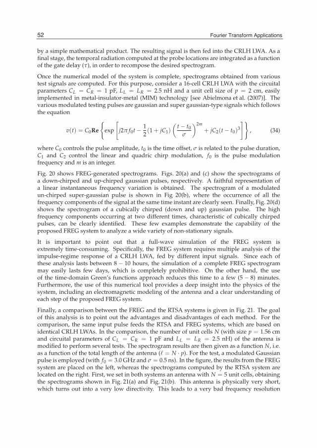
26 Will-be-set-by-IN-TECH
by a simple mathematical product. The resulting signal is then fed into the CRLH LWA. As afinal stage, the temporal radiation computed at the probe locations are integrated as a functionof the gate delay (τ), in order to recompose the desired spectrogram.
Once the numerical model of the system is complete, spectrograms obtained from varioustest signals are computed. For this purpose, consider a 16-cell CRLH LWA with the circuitalparameters CL = CR = 1 pF, LL = LR = 2.5 nH and a unit cell size of p = 2 cm, easilyimplemented in metal-insulator-metal (MIM) technology [see Abielmona et al. (2007)]. Thevarious modulated testing pulses are gaussian and super gaussian-type signals which followsthe equation
v(t) = C0Re
{exp
[j2π f0t− 1
2(1 + jC1)
(t− t0
σ
)2m+ jC2(t− t0)
3
]}, (34)
where C0 controls the pulse amplitude, t0 is the time offset, σ is related to the pulse duration,C1 and C2 control the linear and quadric chirp modulation, f0 is the pulse modulationfrequency and m is an integer.
Fig. 20 shows FREG-generated spectrograms. Figs. 20(a) and (c) show the spectrograms ofa down-chirped and up-chirped gaussian pulses, respectively. A faithful representation ofa linear instantaneous frequency variation is obtained. The spectrogram of a modulatedun-chirped super-gaussian pulse is shown in Fig 20(b), where the occurrence of all thefrequency components of the signal at the same time instant are clearly seen. Finally, Fig. 20(d)shows the spectrogram of a cubically chirped (down and up) gaussian pulse. The highfrequency components occurring at two different times, characteristic of cubically chirpedpulses, can be clearly identified. These few examples demonstrate the capability of theproposed FREG system to analyze a wide variety of non-stationary signals.
It is important to point out that a full-wave simulation of the FREG system isextremely time-consuming. Specifically, the FREG system requires multiple analysis of theimpulse-regime response of a CRLH LWA, fed by different input signals. Since each ofthese analysis lasts between 8 − 10 hours, the simulation of a complete FREG spectrogrammay easily lasts few days, which is completely prohibitive. On the other hand, the useof the time-domain Green’s functions approach reduces this time to a few (5 − 8) minutes.Furthermore, the use of this numerical tool provides a deep insight into the physics of thesystem, including an electromagnetic modeling of the antenna and a clear understanding ofeach step of the proposed FREG system.
Finally, a comparison between the FREG and the RTSA systems is given in Fig. 21. The goalof this analysis is to point out the advantages and disadvantages of each method. For thecomparison, the same input pulse feeds the RTSA and FREG systems, which are based onidentical CRLH LWAs. In the comparison, the number of unit cells N (with size p = 1.56 cmand circuital parameters of CL = CR = 1 pF and LL = LR = 2.5 nH) of the antenna ismodified to perform several tests. The spectrogram results are then given as a function N, i.e.as a function of the total length of the antenna (� = N · p). For the test, a modulated Gaussianpulse is employed (with f0 = 3.0 GHz and σ = 0.5 ns). In the figure, the results from the FREGsystem are placed on the left, whereas the spectrograms computed by the RTSA system arelocated on the right. First, we set in both systems an antenna with N = 5 unit cells, obtainingthe spectrograms shown in Fig. 21(a) and Fig. 21(b). This antenna is physically very short,which turns out into a very low directivity. This leads to a very bad frequency resolution
52 Fourier Transform Applications

Impulse-Regime Analysis of Novel Optically-Inspired Phenomena at Microwaves 27
(a) (b)
(c) (d)
(e) (f)
Fig. 21. Spectrograms obtained by the proposed FREG (figures on the left) and RTSA (figureson the right) systems, based on identical CRLH LWAs for the different tests. The antennas arecomposed of different numbers of N cells, with length p = 1.56 cm and circuital parametersof CL = CR = 1 pF and LL = LR = 2.5 nH. A modulated Gaussian pulse feeds the systems( f0 = 3.0 GHz, σ = 0.5 ns). The resulting spectrograms are given for the case of N = 5 [(a)and (b)], N = 20 [(c) and (d)] and N = 40 [(e) and (f)] unit cells.
53Impulse-Regime Analysis of Novel Optically-Inspired Phenomena at Microwaves

28 Will-be-set-by-IN-TECH
in both spectrograms. On the other hand, this antenna provides an excellent time-gatingtrade-off, because the energy is instantaneously radiated, almost without propagation alongthe structure, leading to a large time resolution. Thereby, the use of a very short antennaleads to generally erroneous spectrograms, due to the wide detection of frequencies whichare not part of the input pulse. Second, we modify the CRLH LWA antenna, including nowa total of N = 20 unit cells. This configuration provides a good frequency resolution inboth systems, while the temporal resolution is deteriorated in the RTSA system (due to theuse of a longer antenna). The resulting spectrograms are depicted on Fig. 21(c) (FREG) andFig. 21(d) (RTSA). As it can be observed, the FREG system provides a completely realisticspectrogram, which faithfully reproduces the input signal in terms of frequency and time(location and spreading). On the other hand, the spectrogram obtained by the RTSA has agood frequency resolution, but has some problems dealing with the temporal duration of thepulse. As previously commented, this problem is due to the propagation of the input pulseas it is being radiated, as graphically illustrated in Fig. 15. And third, we simulate the FREGand RTSA systems based on the same CRLH LWA, but composed now of N = 40 unit cells.The results are shown in Fig. 21(e) (FREG) and Fig. 21(f) (RTSA). The spectrogram obtainedusing the FREG system is quite similar to the previous FREG spectrogram (N = 20 unit cells),keeping the temporal characteristics but improving the frequency resolution (because a longerantenna provides higher directivity). All relevant features of the input modulated Gaussianpulse, in terms of frequency and time, can easily be extracted from this spectrogram. However,the RTSA system provides a completely wrong result. This is because of the excessive lengthof the CRLH LWA, which completely destroy the temporal resolution of the system.
The above comparison demonstrates that the proposed FREG system presents importantadvantages over the RTSA system, specially in terms on temporal resolution, being able tocharacterize any unknown UWB input signal. Furthermore, this comparison has shown thatthe RTSA system can only deal with signals whose frequency and temporal characteristicsare -at least overall- previously known. On the other hand, the main constrains of the FREGsystem are the complex equipment required, the requirement of a periodic input signal, andthe fact that it is not a completely real-time system.
4. Conclusions
This chapter has introduced an impulse-regime analysis of metamaterial-type transmissionlines and antennas. Specifically, a novel formulation, based on Fourier transformations,has been proposed to describe pulse propagation along dispersive linear CRLH lines. Theproposed theory is capable to model complex impulse-regime phenomena, such as dispersion,in a simple, accurate and fast way. Then, the method has been extended to considerCRLH leaky-wave antennas, allowing a fast and accurate analysis of the far-field radiationof these structures in time-domain. The proposed formulation has then been applied tothe development of novel phenomena and applications in the microwave domain, most of themtransported from optics. Instead of the usual magnitude engineering and filter design, adispersion or phase engineering has been applied. In this approach, the dispersive natureand subsequent impulse-regime properties of CRLH structures have been exploited to obtainnovel phenomena/applications. Each phenomenon or application proposed has theoreticallybeen described, numerically verified, and in most of the cases, experimentally demonstrated.The shift from narrow band systems (mostly used in the past) to ultra wide band systems,required by current high date rate wireless communication systems, suggests that the
54 Fourier Transform Applications
Impulse-Regime Analysis of Novel Optically-Inspired Phenomena at Microwaves 29
forthcoming decades will experience a major interest on this dispersive engineering approach,providing new, novel and more exciting effects and devices at microwaves.
5. References
Abielmona, S., Gupta, S. & Caloz, C. (2007). Experimental demonstration and characterizationof a tunable CRLH delay line system for impulse/continuous wave, IEEE Microwaveand Wireless Components Letters 17(12): 864–866.
Abielmona, S., Gupta, S., Nguyen, H. V. & Caloz, C. (2008). Dispersion engineeredimpulse regime memataterial devices, Proc. XXIXth Assembly of Union Radio ScienceInternational (URSI), Chicago, IL, USA.
Amin, G. & Feng, K. D. (1995). Short-time fourier transforms using cascade filterstructures, IEEE Transaction on Circuits and Systems II, Analog Digital Signal Processing20(3): 631–641–408.
Azaña, J. & Muriel, M. A. (1999). Technique for multiplying the repetition rates of periodictrains of pulses by means of a temporal self-imaging effect in chirped fiber gratings,Optics Lett. 24: 1672–1674.
Azaña, J. & Muriel, M. A. (2001). Temporal self-imaging effects: theory and application formultiplying pulse repetition rates, IEEE J. Sel. Top. Quantum Electron 7: 728–744.
Balanis, C. A. (2005). Antenna Theory: Analysis and Design. 3rd Edition., John Wiley and Sons.Barton, G. (1989). Elements of Green’s Functions and Propagation, Oxford Science Publications.Berger, N. K., Levit, B. S., Bekker, A. & Fischer, B. (2004). Compression of periodic
optical pulses using temporal fractional talbot effect, IEEE Photonics Technology Letters16(8): 1855–1857.
Caloz, C. (2009). Perspectives on EM metamaterials, Materials Today 12(3).Caloz, C. & Itoh, T. (2006). Electromagnetic Metamaterials: Transmission Line Theory and
Microwave Applications., Wiley and IEEE Press.Cohen, L. (1989). Time-frequency distributions-a review, Proceedings of the IEEE 77(2): 941–981.Collin, R. E. (1991). Field Theory of Guided Waves, IEEE Press, Piscataway, N.J.Duran-Sindreu, M., Velez, A., Aznar, F., Bonache, J. & Martin, F. (2009). Application of open
split ring resonators and open complementary split ring resonators to the synthesisof artificial transmission lines and microwave passive components, IEEE Transactionson Microwave Theory and Techniques 57(2): 3395–3403.
Eleftheriades, G. (2009). EM transmission-line metamaterials, Materials Today 12(3).Eleftheriades, G. V. & Balmain, K. G. (eds) (2005). Negative-Refraction Metamaterials:
Fundamental Principles and Applications, Wiley & IEEE Press, Hoboken, NJ.Felsen, L. B. (1969). Transients in dispersive media, part I: Theory, IEEE Transactions on
Antennas and Propagation 17: 191–200.Ghavami, M., Michael, L. B. & Kohno, R. (2007). UWB Signals and Systems in Communication
Engineering, J. Wiley & Sons.Gómez-Díaz, J. S., Gupta, S., Álvarez-Melcón, A. & Caloz, C. (2009a). Impulse-regime
CRLH resonator for tunable pulse rate multiplication, Radio Science44(doi:10.1029/2008RS003991): 1–9.
Gómez-Díaz, J. S., Gupta, S., Álvarez-Melcón, A. & Caloz, C. (2009b). Investigationon the phenomenology of impulse-regime metamaterial transmission lines, IEEETransactions on Antennas and Propagation 57(12): 4010–4014.
55Impulse-Regime Analysis of Novel Optically-Inspired Phenomena at Microwaves
30 Will-be-set-by-IN-TECH
Gómez-Díaz, J. S., Gupta, S., Álvarez-Melcón, A. & Caloz, C. (2009c). Tunable talbot imagingdistance using an array of beam-steered metamaterial leaky-wave antennas, Journalof Applied Physics 106: 084908–9.
Gómez-Díaz, J. S., Gupta, S., Álvarez-Melcón, A. & Caloz, C. (2010). Effcient time-domainanálisis of highly-dispersive linear and non-linear metamaterial waveguide andantenna structures, IET Microwaves, Antennas and Propagation 4(10): 1617–1625.
Gupta, S., Abielmona, S. & Caloz, C. (2009). Microwave analog real-time spectrum analyzer(rtsa) based on the spatial-spectral decomposition property of leaky-wave structures,IEEE Transactions on Microwave Theory and Techniques 57(12): 4010–4014.
Gupta, S., Gómez-Díaz, J. S. & Caloz, C. (2009). Frequency resolved electrical gatingprinciple for UWB signal characterization using leaky-wave structures, 39th EuropeanMicrowave Conference, Rome, Italy.
Horii, Y., Caloz, C. & Itoh, T. (2005). Super-compact multilayered left-handed transmissionline and diplexer application, IEEE Transactions on Microwave Theory and Techniques53(4).
Marques, R., Martín, F. & Sorolla, M. (eds) (2008). Metamaterials with Negative Parameters:Theory, Design and Microwave Applications, Wiley, Hoboken, NJ.
Oliner, A. A. & Jackson, D. R. (2007). Leaky-wave antennas, in J. L. Volakis (ed.), AntennaEngineering Handbook, 4 edn, McGraw-Hill, New York.
Oppenheim, A. V. (1996). Signals and Systems, Prentice Hall.Paul, C. R. (2007). Analysis of Multiconductor Transmission Lines, 2nd edition edn, Wiley-IEEE
Press.Pipes, L. A. & Harvill, L. R. (1971). Applied Mathematics for Engineers and Physicist, 3rd edn,
McGraw Hill.Pozar, D. (2005). Microwave Engineering, 3rd edn, John Wiley and Sons.Saleh, B. E. A. & Teich, M. C. (2007). Fundamentals of Photonics, 2nd edition edn,
Wiley-Interscience.Talbot, H. F. (1836). Facts relating to optical science no. IV, Philos. Mag. 9: 401–407.Trebino, R. (ed.) (2002). Frequency-Resolved Optical Gating: The Measurement of Ultrashort Laser
Pulses, Springer.
56 Fourier Transform Applications
3
Fourier Transform Application in the Computation of
Lightning Electromagnetic Field Vesna Javor
University of Nis / Faculty of Electronic Engineering Serbia
1. Introduction Atmospheric discharge is one of the most interesting and powerful natural phenomenon hiding from men its undiscovered features and secrets for centuries. Lightning discharges have been studied in many theoretical and experimental ways. However, application of Fourier transform has been introduced in this research only in recent few decades. It proved very useful in solving many lightning research problems.
There are two main groups of problems in lightning studies that involve using Fourier transform. One deals with determining how the energy is distributed over a continuous frequency spectrum for the quantity of interest. Channel-base currents, induced voltages and currents, electric and magnetic field components, so as integrals and derivatives of the same functions, distribute components over the entire frequency range in different ways. These are non-periodic functions scattering their energy throughout the frequency spectra.
Another important group of problems to be solved by Fourier transform deals with the calculation of lightning induced effects at different distances from the lightning discharge and risk assessment for buildings, various structures, people and property in an external impulse electromagnetic field. These calculations are based on experimental results for the measured lightning electromagnetic field (LEMF) and channel-base currents, which are used in different types of lightning stroke models including lossy ground effects. Lightning discharge channel is usually modeled by a thin vertical antenna at a lossy ground of known electrical parameters. Both ground and air are treated as linear, isotropic and homogeneous half-spaces. Even for such a simple approximation of the lightning channel - calculations can not be easily done in time domain, but transformation to frequency domain is used instead. Once the calculations are done in frequency domain, way back to time domain is made by Inverse Fourier transform applied to the obtained results.
In both groups of problems an impulse function which has the analytical derivative, integral and integral transformations is very useful. New functions proposed by the author for representing lightning currents are presented in this Chapter, Section 2. These can be also used in other high voltage technique calculations. The main problem for a user of the impulse functions already given in literature to approximate some quantity is the choice of parameters so to obtain desired waveshape characteristics or values adequate to

Fourier Transform Applications
58
experimentally measured. Parameters of the new channel-base current (NCBC) function (Javor, 2008; Javor & Rancic, 2011) are calculated according to IEC 62305 standard lightning currents (International Electrotechnical Commission, Technical Committee 81 [IEC, TC 81], 2006), and the procedure to choose function parameters is also explained in (Javor & Rancic, 2011). Functions to represent other typical lightning currents are proposed in (Javor, 2011b, 2011c), such as long stroke current (LSC), and two-rise function (TRF) as a multi-peaked current. These functions can be used to obtain the desired peak value, rise-time, decaying time to half of the peak value, current steepness, integral of the function (representing also impulse charge), or integral of the square of the function (representing also specific energy), etc. Fourier transform is obtained analytically and the results are presented in Section 3. Application of the Fourier transform in LEMF computation is shown in Section 4. Based on these results, some conclusions are given in Section 5.
2. NCBC function Any mathematical function capable to approximate the impulse lightning channel-base current in electromagnetic field calculations can be also used to represent far lightning electromagnetic field as an external excitation inducing currents and voltages in objects and structures inside such a field. Such functions are necessary in lightning stroke modeling.
There is an overview of lightning return-stroke models in (Rakov & Uman, 1998, 2006) where they are classified into four classes according to the type of governing equations. An adequate return-stroke model would be the one that provides simultaneously an approximation to the experimentally measured channel-base current, to the lightning electric and magnetic field waveshapes and intensities at various distances, and to the observed return-stroke speeds. Functions implied in these models are based either on the double-exponential (DEXP) function (Bewley, 1929; Bruce & Golde, 1941) or Heidler’s function (Heidler, 1985). DEXP first order derivative at t=0+ is too large, thus causing numerical problems in LEMF calculations. It also has physically non-realistic convex waveshape in the rising part. Heidler’s function reproduces concave rising part and its derivative is equal to zero at t=0+. It is also used for representing lightning currents in the International standard IEC 62305 (IEC/TC 81, 2006). In order to obtain better agreement with experimental results (Berger et al., 1975) one function was proposed (Nucci et al., 1990) as a linear combination of the DEXP and Heidler’s function. Another pulse function was also proposed in (Feizhou & Shange, 2004). All these functions need peak correction factors, and their parameters cannot be easily chosen according to the desired waveshape. However, NCBC function parameters in the rising part can be chosen independently from parameters in the decaying part. The exact rising time to the peak value can be chosen in advance, and the decaying time to half of the peak value can be selected in the approximation procedure. The maximum value of the function can be chosen without the peak correction factor. Maximum current steepness can be adjusted (Javor & Rancic, 2011) using analytical expression for the first derivative. Experimentally measured impulse charge and specific energy values (Berger et al., 1975; Anderson & Eriksson, 1980) can be achieved using analytically obtained integral of NCBC function and integral of the square of the function (Javor, 2011a).
NCBC function (Fig. 1) is given with the following expression:
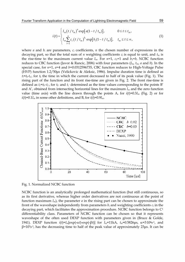
Fourier Transform Application in the Computation of Lightning Electromagnetic Field
59
( ) [ ]
( ) [ ]1
/ exp (1 / ) , 0 ,( )
/ exp (1 / ) , ,i
am m m m
n bm i m i m m
i
I t t a t t t ti t
I c t t b t t t t=
⎧ − ≤ ≤⎪
= ⎨− ≤ ≤ ∞⎪
⎩∑
(1)
where a and bi are parameters, ci coefficients, n the chosen number of expressions in the decaying part, so that the total sum of n weighting coefficients ci is equal to unit, and tm is the rise-time to the maximum current value Im. For n=1, c1=1 and b1=b, NCBC function reduces to CBC function (Javor & Rancic, 2006) with four parameters (Im, tm, a and b). In the special case, for n=1, a=4 and b=0.0312596735, CBC function reduces to High-Voltage Pulse (HVP) function 1.2/50μs (Velickovic & Aleksic, 1986). Impulse duration time is defined as ti=tk-ta’, for tk the time in which the current decreased to half of its peak value (Fig. 1). The rising part of the function and its front rise-time are given in Fig. 2. The front rise-time is defined as tc=tb’-tc’, for tb’ and tc’ determined as the time values corresponding to the points B’ and A’, obtained from intersecting horizontal lines for the maximum Im and the zero function value (time axis) with the line drawn through the points A, for i(t)=0.3Im (Fig. 2) or for i(t)=0.1Im in some other definitions, and B, for i(t)=0.9Im.
Fig. 1. Normalized NCBC function
NCBC function is an analytically prolonged mathematical function (but still continuous, so as its first derivative, whereas higher order derivatives are not continuous at the point of function maximum Im), the parameter a in the rising part can be chosen to approximate the front of the waveshape independently from parameters bi and weighting coefficients ci in the decaying part, which facilitates the approximation procedure. NCBC function belongs to C1 differentiability class. Parameters of NCBC function can be chosen so that it represents waveshape of the often used DEXP function with parameters given in (Bruce & Golde, 1941). DEXP function i(t)=Im[exp(-αt)-exp(-βt)] for Im=11kA, tm=0.5826μs, α=3.104s-1, and β=107s-1, has the decreasing time to half of the peak value of approximately 23μs. It can be
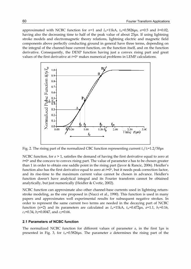
Fourier Transform Applications
60
approximated with NCBC function for n=1 and Im=11kA, tm=0.5826μs, a=0.5 and b=0.02, having also the decreasing time to half of the peak value of about 23μs. If using lightning stroke models and electromagnetic theory relations, lightning electric and magnetic field components above perfectly conducting ground in general have three terms, depending on the integral of the channel-base current function, on the function itself, and on the function derivative. Consequently, the DEXP function having just a convex rising part and great values of the first derivative at t=0+ makes numerical problems in LEMF calculations.
Fig. 2. The rising part of the normalized CBC function representing current tc/ti=1.2/50μs
NCBC function, for a > 1, satisfies the demand of having the first derivative equal to zero at t=0+ and the concave to convex rising part. The value of parameter a has to be chosen greater than 1 in order to obtain one saddle point in the rising part (Javor & Rancic, 2006). Heidler’s function also has the first derivative equal to zero at t=0+, but it needs peak correction factor, and its rise-time to the maximum current value cannot be chosen in advance. Heidler's function doesn't have analytical integral and its Fourier transform cannot be obtained analytically, but just numerically (Heidler & Cvetic, 2002).
NCBC function can approximate also other channel-base currents used in lightning return-stroke modeling, as the one proposed in (Nucci et al., 1990). This function is used in many papers and approximates well experimental results for subsequent negative strokes. In order to represent the same current two terms are needed in the decaying part of NCBC function (n=2) and its parameters are calculated as Im=11kA, tm=0.472μs, a=1.1, b1=0.16, c1=0.34, b2=0.0047, and c2=0.66.
2.1 Parameters of NCBC function
The normalized NCBC function for different values of parameter a, in the first 1μs is presented in Fig. 3, for tm=0.5826μs. The parameter a determines the rising part of the
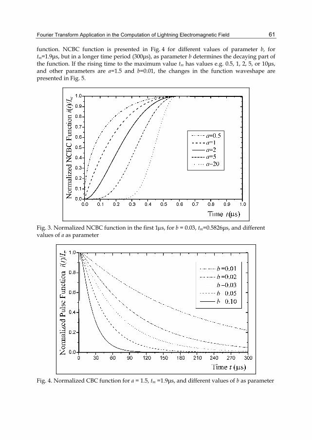
Fourier Transform Application in the Computation of Lightning Electromagnetic Field
61
function. NCBC function is presented in Fig. 4 for different values of parameter b, for tm=1.9μs, but in a longer time period (300μs), as parameter b determines the decaying part of the function. If the rising time to the maximum value tm has values e.g. 0.5, 1, 2, 5, or 10μs, and other parameters are a=1.5 and b=0.01, the changes in the function waveshape are presented in Fig. 5.
Fig. 3. Normalized NCBC function in the first 1μs, for b = 0.03, tm=0.5826μs, and different values of a as parameter
Fig. 4. Normalized CBC function for a = 1.5, tm =1.9μs, and different values of b as parameter

Fourier Transform Applications
62
Fig. 5. Normalized CBC function for a = 1.5, b = 0.01, and different values of tm as parameter
2.2 Derivative of NCBC function
NCBC function first order derivative is:
( ) ( ) [ ]
( ) ( ) [ ]
1
1
1
/ 1 / exp (1 / ) , 0 ,d ( )
d / 1 / exp (1 / ) , ,i
am m m m m
n bm i i m m i m m
i
a I t t t t a t t t ti t
t I c b t t t t b t t t t
−
−
=
⎧ − − ≤ ≤⎪
= ⎨− − ≤ ≤ ∞⎪
⎩∑
(2)
The first derivative of CBC function (NCBC for n=1) is presented in Fig. 6 up to 1μs, for b = 0.03 (but note that parameter b is irrelevant for the rising part), and different values of a, tm and Im.
2.3 Integral of NCBC function
Integral of NCBC function is calculated as:
[ ]
( 1)
( 1)
0
( 1)
1
exp( ) ( 1, / ), 0
exp( ) ( 1, )( )d
exp( ) ( 1, / ) ( 1, ) ,i
am m m m
ta
m m
nb
i i i i i m i i mi
I t a a a at t t t
I t a a a ai t t
c b b b b t t b b t t
− +
− +
− +
=
⎧ γ + ≤ ≤⎪⎪⎪ ⎧⎪ ⎪⎪ γ + += ⎨⎨
⎪⎪⎩⎪
⎪ ⎫⎪⎪ γ + − γ + ≤ ≤ ∞⎬⎪ ⎪⎭⎩
∫
∑
(3)
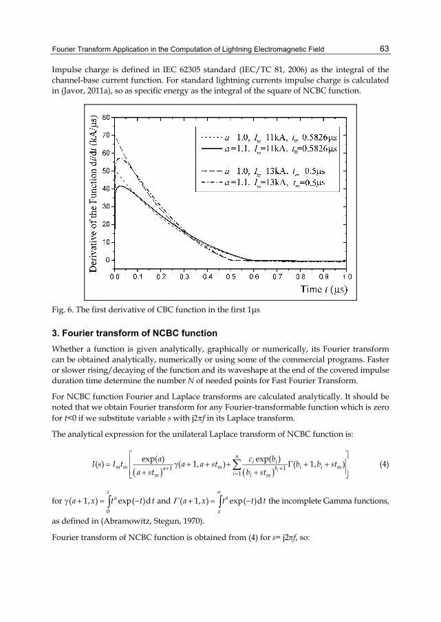
Fourier Transform Application in the Computation of Lightning Electromagnetic Field
63
Impulse charge is defined in IEC 62305 standard (IEC/TC 81, 2006) as the integral of the channel-base current function. For standard lightning currents impulse charge is calculated in (Javor, 2011a), so as specific energy as the integral of the square of NCBC function.
Fig. 6. The first derivative of CBC function in the first 1μs
3. Fourier transform of NCBC function Whether a function is given analytically, graphically or numerically, its Fourier transform can be obtained analytically, numerically or using some of the commercial programs. Faster or slower rising/decaying of the function and its waveshape at the end of the covered impulse duration time determine the number N of needed points for Fast Fourier Transform.
For NCBC function Fourier and Laplace transforms are calculated analytically. It should be noted that we obtain Fourier transform for any Fourier-transformable function which is zero for t<0 if we substitute variable s with j2πf in its Laplace transform.
The analytical expression for the unilateral Laplace transform of NCBC function is:
( ) ( )1 1
1
exp( )exp( )( ) ( 1, ) ( 1, )i
ni i
m m m i i ma bim i m
c baI s I t a a st b b sta st b st+ +
=
⎡ ⎤⎢ ⎥= γ + + + Γ + +⎢ ⎥+ +⎣ ⎦
∑ (4)
for 0
( 1, ) exp( )dx
aa x t t tγ + = −∫ and ( 1, ) exp( )da
x
a x t t tΓ∞
+ = −∫ the incomplete Gamma functions,
as defined in (Abramowitz, Stegun, 1970).
Fourier transform of NCBC function is obtained from (4) for s= j2πf, so:

Fourier Transform Applications
64
( ) ( )1 11
exp( )exp( )( ) ( 1, j2 ) ( 1, j2 )j2 j2 i
ni i
m m m i i ma bim i m
c baI f I t a a f t b b f ta f t b f t
π ππ π+ +
=
⎡ ⎤⎢ ⎥= γ + + + Γ + +⎢ ⎥+ +⎣ ⎦
∑ . (5)
It can be obtained also numerically, or by using some computer program such as FAS (Walker, 1996) with the application of FFT (Fast Fourier Transform). Any frequency domain calculations can be done just for the positive frequencies, as for FFT of real functions the following relations are valid:
{ } { }Re ( ) Re ( )k N kI f I f−= (6)
and
{ } { }Im ( ) Im ( )k N kI f I f−= − . (7)
This feature makes the time for computing FFT twice shorter for real functions, which is very useful if the number of FFT points is great so that calculations are time-consuming. For smaller number of FFT points the computing time is shortened. FFT results given for NCBC function representing lightning current indicate that the major part of its power is in the lower frequency range. The modulus of FFT decays fast as the function of frequency, so it is better to use some other than linear scaling of frequencies in order to cover the lower part of the frequency range. For very high frequencies, the values of real and imaginary parts of FFT of the pulse functions near the end of the frequency interval can be taken as zeros, as they are relatively very small comparing to the values at lower frequencies. That doesn't make much influence on computation results if IFFT (Inverse Fast Fourier Transform) is done for obtaining time domain results based on frequency domain calculations. The sufficient number of FFT points for lightning research studies should be 1024, but better results are obtained with 2048 or 4096 points. This depends on the time interval to cover and the current waveshape.
Fourier transform of Heidler’s function is calculated approximately (Andreotti et al., 2005). Some FFT results for Heidler’s function are also given in (Vujevic & Lovric, 2010). NCBC/CBC have analytical solutions for Fourier transform which enables obtaining analytical solution for LEMF results in the case of perfectly conducting ground.
The modulus of Fourier transform of HVP function 1.2/50μs is presented in Fig. 7, for I(f) normalized to I(0), as the function of log10f. For f2≈6.4kHz≈103.8Hz the normalized modulus of FFT is |I(f2)/I(0)|≈0.3657. The results are obtained for FFT calculated in N=8192 points, for the time step ∆T≈19.064ns, frequency step ∆f≈6.4kHz, and limit frequency fg≈52.455 MHz. From Fig. 7 is obvious that using frequencies higher than a few MHz is not necessary.
For some frequencies up to the chosen limit frequency the results are presented in Table 1 for FFT of HVP function 1.2/50μs calculated in N=8192 points, for ∆T≈19.064ns, ∆f≈6.4kHz, and fg≈52.455MHz. For the chosen number of points for FFT, the corresponding time interval is T=N∆T≈156.17μs and the frequency step is ∆f=(N∆T)-1= T-1. For such values there are 8192 frequencies in the chosen frequency interval [-0.5fg,+0.5 fg], and the highest positive frequency is f4097≈26.2275MHz. FFT results for |I(f)|≈10-n|I(0)| for n=1, 2, 3, …, 8, are also given in Table 1, corresponding approximately to frequencies f5, f35, f108, f352, f2478, f3912, f4078, f4095, and they also point out to the fast decaying of FFT modulus. As (6) and (7) are valid for

Fourier Transform Application in the Computation of Lightning Electromagnetic Field
65
the real functions, this makes the time for computing twice shorter. This is very useful if the number of FFT points is great and relevant calculations in frequency domain are time-consuming. For smaller number of FFT points the total computing time is shortened, but the sampling interval in time domain is critical in that case.
fk f(Hz) Re{I(f)} Im{I(f)} |I(f)/I(0)| f1 0.0000E+00 0.6232E-04 0.0000E+00 0.1000E+01 f2 0.6403E+04 0.6892E-05 -0.2172E-04 0.3657E+00 f3 0.1281E+05 0.8713E-06 -0.1179E-04 0.1896E+00 f4 0.1921E+05 -0.2839E-06 -0.7867E-05 0.1263E+00 f5 0.2561E+05 -0.6610E-06 -0.5842E-05 0.9433E-01 f35 0.2177E+06 -0.6334E-06 -0.6164E-07 0.1021E-01 f108 0.6851E+06 0.4510E-07 0.4597E-07 0.1033E-02 f352 0.2248E+07 0.4931E-09 0.6259E-08 0.1007E-03 f2478 0.1586E+08 0.8158E-12 0.6237E-09 0.1001E-04 f3912 0.2503E+08 -0.2014E-12 0.6261E-10 0.1005E-05 f4078 0.2611E+08 -0.1417E-12 0.6350E-11 0.1019E-06 f4095 0.2621E+08 -0.1377E-12 0.6689E-12 0.1096E-07 f4097 0.2623E+08 -1.3765E-13 0.0000E+00 2.2088E-09
Table 1. FFT of the HVP function in 8196 points
Fig. 7. Normalized FFT modulus of HVP as the function of frequency
For example, for N=2048 and the same time interval T=N∆T≈156.172μs the sampling frequency is fg=1/∆T≈13.114MHz, which gives the same frequency step ∆f≈6.4kHz, but four times greater step in time domain ∆T≈76.256ns than if N=8092.
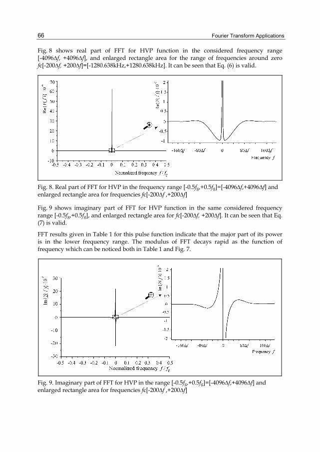
Fourier Transform Applications
66
Fig. 8 shows real part of FFT for HVP function in the considered frequency range [-4096∆f, +4096∆f], and enlarged rectangle area for the range of frequencies around zero fє[-200∆f, +200∆f]=[-1280.638kHz,+1280.638kHz]. It can be seen that Eq. (6) is valid.
Fig. 8. Real part of FFT for HVP in the frequency range [-0.5fg,+0.5fg]=[-4096∆f,+4096∆f] and enlarged rectangle area for frequencies fє[-200∆f ,+200∆f]
Fig. 9 shows imaginary part of FFT for HVP function in the same considered frequency range [-0.5fg,+0.5fg], and enlarged rectangle area for fє[-200∆f, +200∆f]. It can be seen that Eq. (7) is valid.
FFT results given in Table 1 for this pulse function indicate that the major part of its power is in the lower frequency range. The modulus of FFT decays rapid as the function of frequency which can be noticed both in Table 1 and Fig. 7.
Fig. 9. Imaginary part of FFT for HVP in the range [-0.5fg,+0.5fg]=[-4096∆f,+4096∆f] and enlarged rectangle area for frequencies fє[-200∆f ,+200∆f]
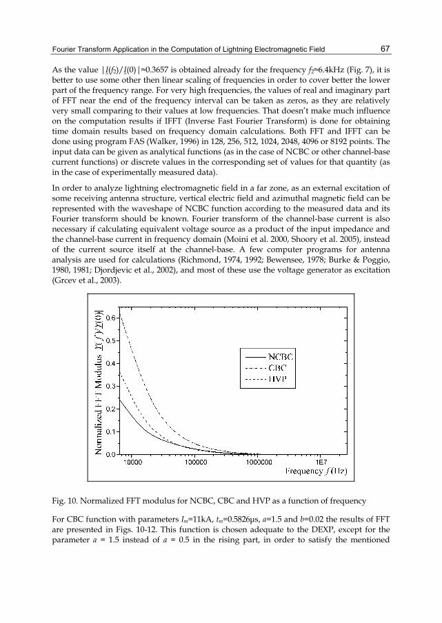
Fourier Transform Application in the Computation of Lightning Electromagnetic Field
67
As the value |I(f2)/I(0)|≈0.3657 is obtained already for the frequency f2≈6.4kHz (Fig. 7), it is better to use some other then linear scaling of frequencies in order to cover better the lower part of the frequency range. For very high frequencies, the values of real and imaginary part of FFT near the end of the frequency interval can be taken as zeros, as they are relatively very small comparing to their values at low frequencies. That doesn’t make much influence on the computation results if IFFT (Inverse Fast Fourier Transform) is done for obtaining time domain results based on frequency domain calculations. Both FFT and IFFT can be done using program FAS (Walker, 1996) in 128, 256, 512, 1024, 2048, 4096 or 8192 points. The input data can be given as analytical functions (as in the case of NCBC or other channel-base current functions) or discrete values in the corresponding set of values for that quantity (as in the case of experimentally measured data).
In order to analyze lightning electromagnetic field in a far zone, as an external excitation of some receiving antenna structure, vertical electric field and azimuthal magnetic field can be represented with the waveshape of NCBC function according to the measured data and its Fourier transform should be known. Fourier transform of the channel-base current is also necessary if calculating equivalent voltage source as a product of the input impedance and the channel-base current in frequency domain (Moini et al. 2000, Shoory et al. 2005), instead of the current source itself at the channel-base. A few computer programs for antenna analysis are used for calculations (Richmond, 1974, 1992; Bewensee, 1978; Burke & Poggio, 1980, 1981; Djordjevic et al., 2002), and most of these use the voltage generator as excitation (Grcev et al., 2003).
Fig. 10. Normalized FFT modulus for NCBC, CBC and HVP as a function of frequency
For CBC function with parameters Im=11kA, tm=0.5826μs, a=1.5 and b=0.02 the results of FFT are presented in Figs. 10-12. This function is chosen adequate to the DEXP, except for the parameter a = 1.5 instead of a = 0.5 in the rising part, in order to satisfy the mentioned
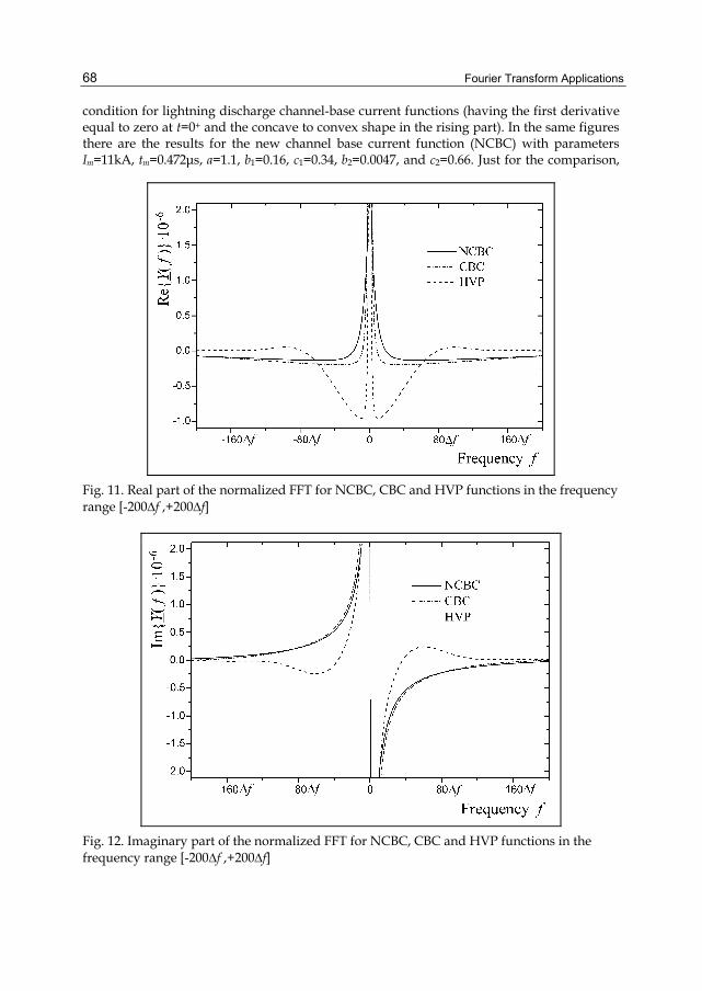
Fourier Transform Applications
68
condition for lightning discharge channel-base current functions (having the first derivative equal to zero at t=0+ and the concave to convex shape in the rising part). In the same figures there are the results for the new channel base current function (NCBC) with parameters Im=11kA, tm=0.472μs, a=1.1, b1=0.16, c1=0.34, b2=0.0047, and c2=0.66. Just for the comparison,
Fig. 11. Real part of the normalized FFT for NCBC, CBC and HVP functions in the frequency range [-200∆f ,+200∆f]
Fig. 12. Imaginary part of the normalized FFT for NCBC, CBC and HVP functions in the frequency range [-200∆f ,+200∆f]
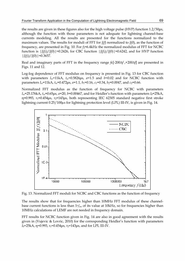
Fourier Transform Application in the Computation of Lightning Electromagnetic Field
69
the results are given in these figures also for the high voltage pulse (HVP) function 1.2/50μs, although the function with those parameters is not adequate for lightning channel-base currents modeling. All the results are presented for the functions normalized to the maximum values. The results for moduli of FFT for I(f) normalized to I(0), as the function of frequency, are presented in Fig. 10. For f2≈6.4kHz the normalized modulus of FFT for NCBC function is |I(f2)/I(0)|≈0.2426, for CBC function |I(f2)/I(0)|≈0.6242, and for HVP function |I(f2)/I(0)|≈0.3657.
Real and imaginary parts of FFT in the frequency range fє[-200∆f ,+200∆f] are presented in Figs. 11 and 12.
Log-log dependence of FFT modulus on frequency is presented in Fig. 13 for CBC function with parameters Im=11kA, tm=0.5826μs, a=1.5 and b=0.02 and for NCBC function with parameters Im=11kA, tm=0.472μs, a=1.1, b1=0.16, c1=0.34, b2=0.0047, and c2=0.66.
Normalized FFT modulus as the function of frequency for NCBC with parameters Im=25.176kA, tm=0.65μs, a=20, b=0.00467, and for Heidler’s function with parameters I0=25kA, η=0.993, τ1=0.454μs, τ2=143μs, both representing IEC 62305 standard negative first stroke lightning current 0.25/100μs for lightning protection level (LPL) III-IV, is given in Fig. 14.
Fig. 13. Normalized FFT moduli for NCBC and CBC functions as the function of frequency
The results show that for frequencies higher than 10MHz FFT modulus of these channel-base current functions is less than 1o/oo of its value at 10kHz, so for frequencies higher than 10MHz calculations of LEMF are not needed in frequency domain.
FFT results for NCBC function given in Fig. 14 are also in good agreement with the results given in (Vujevic & Lovric, 2010) for the corresponding Heidler’s function with parameters I0=25kA, η=0.993, τ1=0.454μs, τ2=143μs, and for LPL III-IV.
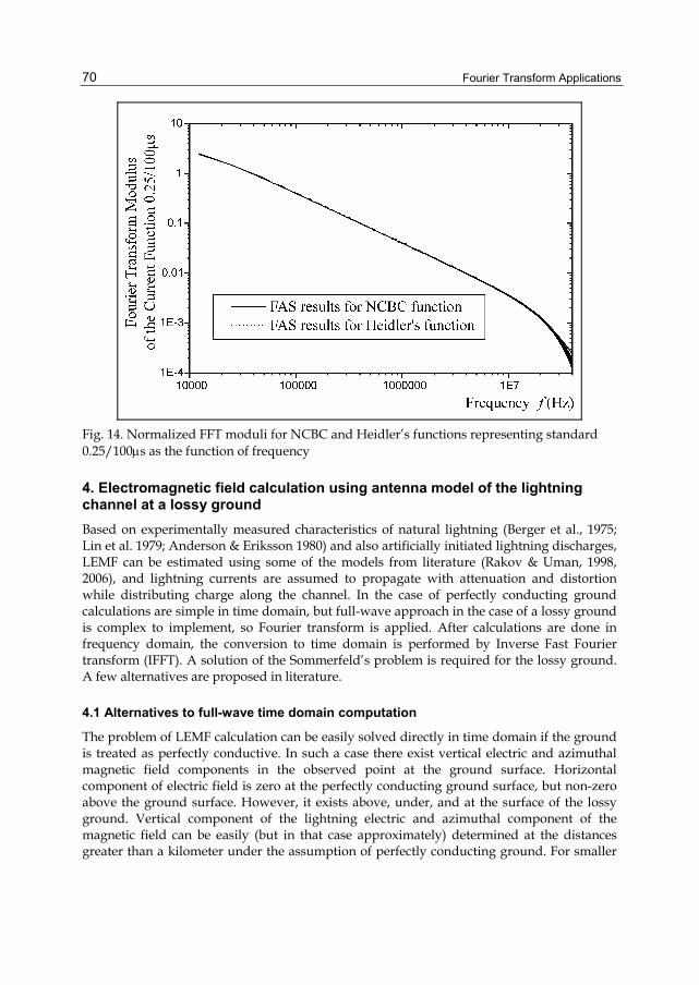
Fourier Transform Applications
70
Fig. 14. Normalized FFT moduli for NCBC and Heidler’s functions representing standard 0.25/100μs as the function of frequency
4. Electromagnetic field calculation using antenna model of the lightning channel at a lossy ground Based on experimentally measured characteristics of natural lightning (Berger et al., 1975; Lin et al. 1979; Anderson & Eriksson 1980) and also artificially initiated lightning discharges, LEMF can be estimated using some of the models from literature (Rakov & Uman, 1998, 2006), and lightning currents are assumed to propagate with attenuation and distortion while distributing charge along the channel. In the case of perfectly conducting ground calculations are simple in time domain, but full-wave approach in the case of a lossy ground is complex to implement, so Fourier transform is applied. After calculations are done in frequency domain, the conversion to time domain is performed by Inverse Fast Fourier transform (IFFT). A solution of the Sommerfeld’s problem is required for the lossy ground. A few alternatives are proposed in literature.
4.1 Alternatives to full-wave time domain computation
The problem of LEMF calculation can be easily solved directly in time domain if the ground is treated as perfectly conductive. In such a case there exist vertical electric and azimuthal magnetic field components in the observed point at the ground surface. Horizontal component of electric field is zero at the perfectly conducting ground surface, but non-zero above the ground surface. However, it exists above, under, and at the surface of the lossy ground. Vertical component of the lightning electric and azimuthal component of the magnetic field can be easily (but in that case approximately) determined at the distances greater than a kilometer under the assumption of perfectly conducting ground. For smaller

Fourier Transform Application in the Computation of Lightning Electromagnetic Field
71
distances, propagation above ground of finite conductivity results in the noticeable attenuation of the high-frequency components of electric and magnetic field, and thus in appearance of the horizontal electric field at the surface. Finite conductivity has greater impact on horizontal than on vertical electric field, so calculation of horizontal component requires rigorous computation or, at least, acceptable approximations.
Approximate formulas in frequency domain are often used for calculation of the horizontal electric field in air, up to heights of tens of meters above the ground surface. These formulas can be integrated in the calculation of LEMF in time domain, but the obtained expressions are much more complex. There are simple approximations: the assumption of perfectly conducting ground, "wavetilt" formula, Cooray’s approach and Rubinstein's approach. Cooray, 1992, proposed the calculation of horizontal electric field at the surface of finitely conductive ground using azimuthal magnetic induction and the expression for ground surface impedance. He showed that this simple formula provides very accurate results at the distances of about 200m. Rubinstein, 1996, proposed expression for the horizontal electric field with two terms: 1) horizontal electric field calculated under the assumption of perfectly conducting ground, and 2) the correction factor, given as a product of the magnetic field calculated under the same assumption and the function similar as in “wavetilt” formula which represents the effect of finite conductivity. The basic assumption of Rubinstein's approximation is σ1>>ε0εr1, and that finite ground conductivity does not affect the horizontal magnetic field at the surface. If this is not the case, then more general formula can be written, known in literature as the Cooray-Rubinstein's formula (Cooray, 2002). Wait gave generalization of Cooray-Rubinstein's formula and the exact evaluation of horizontal electric field, showing under which circumstances this general expression reduces to Cooray-Rubinstein's formula (Wait, 1997). Cooray and Lindquist, 1983, and Cooray, 1987, using the attenuation function in time domain proposed by Wait, 1956, included effects of the finite conductivity, and obtained results for the electric field that are in better agreement with experiments. Terms for approximate formulas in time domain are complex, so the approach in frequency domain is preferred.
4.2 Method of images
Method of images gives an approximate solution to the Sommerfeld’s integral. Complex image technique often uses one or more terms of exponential series to approximate plane wave reflection coefficient. Thus, multiple discrete and/or continuous image sources are introduced, and this technique also proved not to be limited to a quasi-static range alone. Using this technique, different authors (Shubair & Chow, 1993; Yang & Zhou, 2004; Popovic & Petrovic, 1993; and Petrovic, 2005) obtained results for Sommerfeld’s integral kernel for vertical dipoles above a lossy half-space which were used for the comparison with the new Two-image approximation (TIA). Approximate formulas are often valid for a limited range of ground electrical parameters, field point distances, or heights of dipoles above ground, but TIA approximation of Sommerfeld’s integral kernel proposed in (Rancic & Javor, 2006 & 2007) has the advantage of being valid in a wide range of lossy ground electrical parameters, for various heights of vertical electric dipoles above the ground, and for possibility to calculate electromagnetic field in both near and far zone.
LEMF can be calculated using thin wire antenna modeling of a lightning channel assumed as vertical, without branches and reflections from the end. If using electromagnetic model,

Fourier Transform Applications
72
boundary conditions are fulfilled at the wire antenna surface, and a voltage or current source is assumed at the channel-base. Unknown current distribution along the antenna is determined by solving some system of integro-differential equations of EFIE or MFIE type satisfying boundary condition for electric or magnetic field components, respectively. One of those is e.g. System of integral equations of two potentials (SIE-TP), (Rancic, 1995), which is of EFIE type. Current distribution along the antenna can be approximated e.g. by polynomials (Popovic, 1970) with unknown complex coefficients. These can be determined by using Method of Moments (MoM) (Harrington, 1968) i.e. by matching in a sufficient number of points along the antenna. Based on that current distribution LEMF is calculated using electromagnetic theory relations. Thus, the problem is solved in full (without mentioned approximations of some LEMF components using others) on the basis of approximate solution of Sommerfeld's problem of a dipole radiating at the arbitrary height above the lossy half-space, which is a classical problem in electromagnetics.
The problem of a dipole radiation in the presence of a lossy medium was noticed yet in 1909, by Sommerfeld, who determined the solution in the form of superposition of inhomogeneous plane waves. His work had such a great influence on later theoretical research in this area that the solution of more complex problems which shows the influence of a lossy medium on the properties of linear antennas is marked as Sommerfeld's solution. Sommerfeld was the first who treated all four cases of elementary Hertz's dipoles in the air applying his formulation through the cylindrical waves. Van der Pol, 1931, proposed approximate method for solving Sommerfeld's integrals. Class of integrals obtained by Sommerfeld's formulation which strictly defines boundary conditions on the surface of discontinuity is known in literature as “integrals of Sommerfeld’s type”. These integrals have limits of integration 0 and infinity, and the integrand is a product of Bessel's function (J0 or J1), exponential, and one more function, so it is of very complex shape. Depending on the complexity of the model, this function has different forms so that different problems appear in its numerical integration. Since these integrals are highly oscillatory and slowly decreasing functions they don’t have solutions in the closed form. In the analysis of antennas above lossy media, there is an inevitable and major problem to determine Sommerfeld's integral as accurate as possible in a wide range of values of electrical parameters of the medium, for different positions of current elements, different frequencies and positions of the observed point in the field. There are many different ways to approximate Sommerfeld's integral which can be found in literature. The model that includes complex mathematical functions in the case of lossy ground gives result equivalent to the field of infinite number of current images. Simpler approximations have limitations as for the values of electrical parameters of the medium, the position of the point in the field (near or far zone) and positions of matching points near or at the interface of two half-spaces. In order to include the influence of electrical parameters of a real ground on antenna characteristics, direct Sommerfeld's approach to the problem can be also used, but it is very complex for solving from both the analytical and numerical point of view. In addition to the direct approach to this problem, it is possible to modify the path of integration of Sommerfeld’s integral, or to use interpolation and speed up the calculation, or to use tables of Sommerfeld's integrals, but there were also some attempts to solve the problem by obtaining approximations in closed form for some special cases of Sommerfeld's integrals. A suitable solution would be the one to determine efficiently Sommerfeld's integrals for arbitrary positions and orientations of dipoles, arbitrary positions of the points in LEMF and a wide range of frequencies.
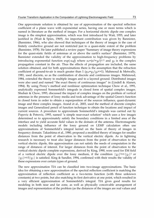
Fourier Transform Application in the Computation of Lightning Electromagnetic Field
73
One approximate solution is obtained by use of approximation of the spectral reflection coefficient of a plane wave with exponential series, having one or more terms which is named in literature as the method of images. For a horizontal electric dipole one complex image is the simplest approximation, which was first introduced by Wait, 1955, and later justified in (Wait & Spies, 1969). An important contribution was given by Bannister, (Bannister, 1966), who also showed that techniques of the theory of images in the case of finitely conductive ground are not restricted just to a quasi-static extent of the problem (Bannister, 1978). He later published a review paper "Summary of image theory expressions for the quasi-static fields of antennas at or above the earth's surface" (Bannister, 1979). Bannister extended the validity of the approximation to high-frequency problems by introducing exponential function exp(-u0d) where u0=(α2+γ02)1/2 and γ0 is the complex propagation constant in the air. Thus the effects of propagation are included, the same solution obtained, and for both approximations there is the assumption that the refraction coefficient of ground-to-air is much greater than 1 (n10=γ1/γ0>>1). Mahmoud & Metwally, 1981, used discrete, so as the combination of discrete and continuous images. Mahmoud, 1984, extended the theory to multiple images and to a layered ground. Distributed images were also used and named “the exact theory of continuous images” in (Lindell & Alanen, 1984). By using Prony’s method and nonlinear optimization technique Chow et al., 1991, analytically expressed Sommerfeld's integrals in closed form of spatial complex images. Shubair & Chow, 1993, discussed the impact of complex images on the problem of vertical antennas in the presence of lossy media and took advantage of the spatial Green's function in closed form in order to obtain a superposition of the sources influence, quasi-dynamic image and three complex images. Arand et al., 2003, used the method of discrete complex images and Generalized pencil of function technique to obtain the locations and impact of current sources. A procedure to approximate Sommerfeld’s integrals was carried out by Popovic & Petrovic, 1993, named "a simple near-exact solution" which uses a few images determined so to approximately satisfy the boundary conditions in a limited area of the interface and to yield accurate field values in the domain of the antenna. Electromagnetic models including influence of the lossy ground on LEMF calculation often use approximations of Sommerfeld’s integral kernel on the basis of theory of images in frequency domain. Takashima et al., 1980, proposed a modified theory of images for smaller distances from the point of observation to the vertical electric dipole. As in lightning research is necessary to treat also larger distances from the point of observation to the vertical electric dipole, this approximation can not satisfy the needs of computation in the range of distances of interest. For larger distances from the point of observation to the vertical electric dipole complete expressions, derived by King, 1990, were used for EM field of a vertical electric dipole over the lossy medium, if the condition |γ2|2>>|γ1|2 or |γ2|>>3|γ1| is satisfied. King & Sandler, 1994, confirmed with their results the validity of these expressions over certain types of ground.
The new approximation TIA can be classified into two-image approximations. The basic idea for obtaining a new approximation of the spectral reflection coefficient is matching the approximation of reflection coefficient as a two-terms function (with three unknown constants) at two points, but also matching its first derivative at one point, which resulted in a very efficient approximation of Sommerfeld's integral. TIA gives good results for modeling in both near and far zone, as well as physically conceivable arrangement of images and representation of the problem (as the distances of the images are real values and
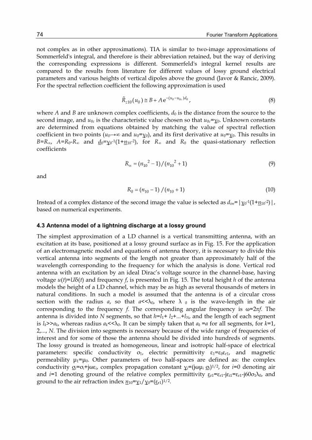
Fourier Transform Applications
74
not complex as in other approximations). TIA is similar to two-image approximations of Sommerfeld's integral, and therefore is their abbreviation retained, but the way of deriving the corresponding expressions is different. Sommerfeld's integral kernel results are compared to the results from literature for different values of lossy ground electrical parameters and various heights of vertical dipoles above the ground (Javor & Rancic, 2009). For the spectral reflection coefficient the following approximation is used
0 0 0( )10 0( ) e ,cu u d
zR u B A − −≅ + (8)
where A and B are unknown complex coefficients, d0 is the distance from the source to the second image, and u0c is the characteristic value chosen so that u0c=γ0. Unknown constants are determined from equations obtained by matching the value of spectral reflection coefficient in two points (u0→∞ and u0=γ0), and its first derivative at u0=γ0. This results in B=R∞, A=R0-R∞ and d0=γ0-1(1+n10-2), for R∞ and R0 the quasi-stationary reflection coefficients
2 210 10( 1)/( 1)R n n∞ = − + (9)
and
0 10 10( 1) /( 1)R n n= − + (10)
Instead of a complex distance of the second image the value is selected as dim=|γ0-1(1+n10-2)|, based on numerical experiments.
4.3 Antenna model of a lightning discharge at a lossy ground
The simplest approximation of a LD channel is a vertical transmitting antenna, with an excitation at its base, positioned at a lossy ground surface as in Fig. 15. For the application of an electromagnetic model and equations of antenna theory, it is necessary to divide this vertical antenna into segments of the length not greater than approximately half of the wavelength corresponding to the frequency for which the analysis is done. Vertical rod antenna with an excitation by an ideal Dirac’s voltage source in the channel-base, having voltage u(t)=Uδ(t) and frequency f, is presented in Fig. 15. The total height h of the antenna models the height of a LD channel, which may be as high as several thousands of meters in natural conditions. In such a model is assumed that the antenna is of a circular cross section with the radius a, so that a<<λ0, where λ 0 is the wave-length in the air corresponding to the frequency f. The corresponding angular frequency is ω=2πf. The antenna is divided into N segments, so that h=l1+ l2+...+lN, and the length of each segment is lk>>ak, whereas radius ak<<λ0. It can be simply taken that ak =a for all segments, for k=1, 2,..., N. The division into segments is necessary because of the wide range of frequencies of interest and for some of those the antenna should be divided into hundreds of segments. The lossy ground is treated as homogeneous, linear and isotropic half-space of electrical parameters: specific conductivity σ1, electric permittivity ε1=ε0εr1, and magnetic permeability μ1=μ0. Other parameters of two half-spaces are defined as: the complex conductivity σi=σi+jωεi, complex propagation constant γi=(jωμi σi)1/2, for i=0 denoting air and i=1 denoting ground of the relative complex permittivity εr1=εr1-jεi1=εr1-j60σ1λ0, and ground to the air refraction index n10=γ1/γ0=(εr1)1/2.
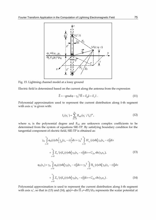
Fourier Transform Application in the Computation of Lightning Electromagnetic Field
75
Fig. 15. Lightning channel model at a lossy ground
Electric field is determined based on the current along the antenna from the expression
20 ˆ ˆgrad zE E E zρ= − ϕ − γ Π = ρ + . (11)
Polynomial approximation used to represent the current distribution along k-th segment with axis sk’ is given with:
, ,
0( ) ( / ) ,
knm
k k mk k km
I s B s l=
= ∑ (12)
where nk is the polynomial degree and Bmk are unknown complex coefficients to be determined from the system of equations SIE-TP. By satisfying boundary condition for the tangential component of electric field, SIE-TP is obtained as:
[ ]20 0 0 00
0 0
( )ch ( ) d ( )sh ( ) dn n
n
s s
n s ns s
s s s s s s s sΠ= =
⎡ ⎤γ ϕ γ − + γ γ −⎣ ⎦∫ ∫
[ ]0 2 00
'( ) ( )sh ( ) d sh( ),ns
n n n n ns
Z s I s s s s C s=
+ γ − = γ∫ (13)
[ ] [ ]20 0 0 0 0 0
0 0
( ) ( )sh ( ) d ( )ch ( ) dn n
n
s s
n n s ns s
s s s s s s s s s= =
ϕ + γ ϕ γ − + γ Π γ −∫ ∫
[ ]0 2 00
'( ) ( )ch ( ) d ch( )ns
n n n n ns
Z s I s s s s C s=
+ γ − = γ∫ . (14)
Polynomial approximation is used to represent the current distribution along k-th segment with axis sk’, so that in (13) and (14), φ(s)=-div Π 0=-∂П/∂z0 represents the scalar potential at

Fourier Transform Applications
76
the antenna surface, Пsn(s)= Пz0(s) Hertz vector tangential component, whereas Zn’(s) is the impedance per unit length, sn the matching point, and s the local coordinate along the n-th conductor, so that 0≤s≤ ln. Пz0(s) and φ0(s) are potentials in the upper half-space to be calculated from:
0 0 1 00 210 ' 0
1( ) ( )[ ( ) ( )]d4 σ
k
k
lNv
z k k k k kk s
s I s K r S r sπ = =
′ ′Π = +∑ ∫ , (15)
0 0 1 00 210 ' 0
1( ) ( ) [ ( ) ( )]d4 σ
k
k
lNv
k k k k kkk s
s I s K r S r ss= =
∂′ ′ϕ = −′π ∂∑ ∫ , (16)
for K0(r1k)=exp(-γ0r1k)/r1k the standard potential kernel, and S00ν (r2k) the Sommerfeld’s integral kernel defined as
00 2 10 0 20
( ) ( ) ( , )d .vk z kS r R K r
α
∞
=
= α α α∫ (17)
10( )zR α is the reflection coefficient in the spectral domain, for the variable 0≤α<∞, so that
2
10 0 110 10 0 2
10 0 1( ) ( ) ,z z
n u uR R un u u
−α = =
+ (18)
for 2 2 2 2 21 1 0 1 0 ,u u= α + γ = + γ − γ and 2 2
0 0 ,u = α + γ whereas 0 2( , )kK rα is the spectral form of the standard potential kernel
0 ( ')
0 2 00
e( , ) ( ρ)ku z s
kK r Ju
− +
α = α α (19)
and
0 2
0 2 0 22 α 0
( ) ( , )d ,kr
k kk
eK r K rr
∞−γ
=
= = α α∫ (20)
for 2 22 ρ ( ')k kr z s= + + the distance from the field point M (ρ, ψ, z) to the first image of the
k-th antenna segment for 2 2ρ x y= + , and 0( ρ)J α the Bessel function of the first kind and order zero.
Thus, for the Sommerfeld’s integral kernel (7) is obtained:
00 2 0 2 0 0 3( ) ( ) exp( ) ( ),vk k im kS r BK r A d K r≅ + γ (21)
for 2 23 ρ ( ' )k k imr z s d= + + + the distance from the second image to the field point, and
0 3 0 3 3( ) exp( ) /k k kK r r r= −γ .
LEMF calculations were also done for the antenna models of cage structures (Javor, 2003) and in the case of lightning protection rods at a lossy ground (Javor & Rancic, 2009).

Fourier Transform Application in the Computation of Lightning Electromagnetic Field
77
4.4 Current distribution along the vertical antenna at the lossy ground
The results obtained with TIA approximation are shown in Fig. 16 for real and imaginary part of the current along the vertical antenna having height h=300m, radius a=0.05m, and resistivity per unit length R’=0.1Ω/m, at the lossy ground of relative dielectric constant εr1=2 and εr1=10, specific conductivity σ1=10-1S/m or 10-5S/m, for frequency f=3MHz, the number of antenna segments N=30, and the degree of polynomial approximation nk =3, for k=1,...,30.
Fig. 16. Real and imaginary part of the current along the antenna for h=300m and radius a=0.05m, for different lossy ground parameters and f=3MHz
4.5 Input impedance of a vertical antenna modeling the lightning discharge channel
Input impedance, Zul, is important for the antenna analysis in frequency domain and presents integral characteristic of the antenna structure, which also allows checking the accuracy of TIA for Sommerfeld's integral kernel. Satisfactory agreement for the polynomial degree n>2 was confirmed. It is enough to choose a polynomial degree n=2 if the length of the antenna is not greater than 0.6λ0, for N=1 segment of the antenna. The polynomial degree should not take values n>8 as the polynomial approximation of the antenna current is not appropriate for those. For σ1λ0<10-1 the obtained values for the input impedance/admittance are not dependent on the normalized conductivity, but approximately equal to the values of the input impedance/admittance in the case of a perfect dielectric of relative dielectric constant εr1.
For the antenna of length h=2600m the results for input impedance are obtained for the frequency step Δf =6.425kHz and the selected maximum frequency fmax/2=3.2896MHz for FFT transforming time interval [0,t] into the frequency interval [-fmax/2, fmax/2]. For an arbitrary overall height h the segmentation should be done depending on the frequency i.e. wavelength into the segments of length lk≤ λ0/2 for a selected polynomial degree nk=3. For frequencies f <500kHz the antenna can be treated as one segment, so that N=1 is enough for calculations, whereas for higher frequencies is necessary to divide the antenna into segments. E.g. about 20 segments are required for frequencies around 1MHz, and about 200 segments for frequencies around 10MHz, if the chosen polynomial degree of the current approximation is nk=3 along each of the segments. Fig. 17 shows the results for input resistance and input reactance of the antenna modeling lightning discharge channel, for

Fourier Transform Applications
78
h=2600m, a=5cm, Z’=0.1 Ω/m, εr1=10 and σ1=0.01S/m, NFFT=1024 points for FFT and Δf=6.425kHz. Fig. 18 shows the results for input conductance and input susceptance. For different frequencies, different number of segments along the VMA in the range 1≤N≤200 was chosen, depending on the observed frequency.
Fig. 17. Input resistance and reactance of the vertical antenna, for h=2600m, a=0.05m, and Z’=0.1Ω/m, at the lossy ground of parameters εr1=10 and σ1=0.01S/m, versus frequency
Fig. 18. Input conductance and susceptance of the vertical antenna, for h=2600m, a=0.05m, and Z’=0.1Ω/m, at the lossy ground of parameters εr1=10 and σ1=0.01S/m, versus frequency
4.6 Frequency domain results for lightning electric field
Results for vertical and radial electric field as functions of the normalized radial distance β0ρ for the normalized antenna height h/λ0=0.25, normalized radius of the antenna a/λ0=0.0005 at the ground of specific conductivity σ1=0.01S/m and for different values of electric permittivity εr1 as parameter, are presented in Fig. 19, and for εr1=10 and for different values of specific conductivity σ1 as parameter in Fig. 20. Vertical and radial component of the electric field at radial distances r from 50 to 250m (0.5λ0≤r≤2.5λ0) from

Fourier Transform Application in the Computation of Lightning Electromagnetic Field
79
Fig. 19. Vertical and radial electric field of the quarter-wavelength monopole antenna at the lossy ground, for σ1=0.01S/m and εr1 as parameter, as functions of normalized distance
Fig. 20. Vertical and radial electric field of the quarter-wavelength monopole antenna at the lossy ground, for εr1=10 and σ1 as parameter, as the functions of normalized distance
the base of the antenna having height h=300m, circular cross section of radius a=5cm at the ground surface of parameters εr1=10 and σ1=0.01S/m, for the frequency f=3MHz, the polynomial degree of the current distribution approximation along each of the segments nk=3, and the number of segments 20, 30 and 50, is presented in Fig. 21. The results obtained for the electric field in the points at a height z=1.5m above the ground surface, for the radial distances 0.5λ0≤r≤2.5λ0, differ a little from results for the field at the ground surface (z=0).
4.7 Time domain results for lightning electromagnetic field
Results for vertical electric and azimuthal magnetic field components are presented in Figs. 22-24 for different distances from the channel-base: r=500m, 5km and 100km. For CBC
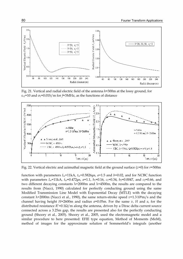
Fourier Transform Applications
80
Fig. 21. Vertical and radial electric field of the antenna h=300m at the lossy ground, for εr1=10 and σ1=0.01S/m for f=3MHz, as the functions of distance
Fig. 22. Vertical electric and azimuthal magnetic field at the ground surface (z=0) for r=500m
function with parameters Im=11kA, tm=0.5826μs, a=1.5 and b=0.02, and for NCBC function with parameters Im=11kA, tm=0.472μs, a=1.1, b1=0.16, c1=0.34, b2=0.0047, and c2=0.66, and two different decaying constants λ=2000m and λ=4500m, the results are compared to the results from (Nucci, 1990) calculated for perfectly conducting ground using the same Modified Transmission Line Model with Exponential Decay (MTLE) with the decaying constant λ=2000m (Nucci et al., 1990), the same return-stroke speed v=1.3.108m/s and the channel having height H=2600m and radius a=0.05m. For the same v, H and a, for the distributed resistance R’=0.1Ω/m along the antenna, driven by a Dirac delta current source connected across a 3.25m gap, the results are presented also for the perfectly conducting ground (Shoory et al., 2005). Shoory et al., 2005, used the electromagnetic model and a similar procedure to here presented: EFIE type equation, Method of Moments (MoM), method of images for the approximate solution of Sommerfeld’s integrals (another
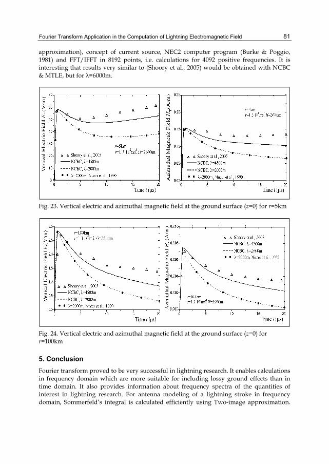
Fourier Transform Application in the Computation of Lightning Electromagnetic Field
81
approximation), concept of current source, NEC2 computer program (Burke & Poggio, 1981) and FFT/IFFT in 8192 points, i.e. calculations for 4092 positive frequencies. It is interesting that results very similar to (Shoory et al., 2005) would be obtained with NCBC & MTLE, but for λ=6000m.
Fig. 23. Vertical electric and azimuthal magnetic field at the ground surface (z=0) for r=5km
Fig. 24. Vertical electric and azimuthal magnetic field at the ground surface (z=0) for r=100km
5. Conclusion Fourier transform proved to be very successful in lightning research. It enables calculations in frequency domain which are more suitable for including lossy ground effects than in time domain. It also provides information about frequency spectra of the quantities of interest in lightning research. For antenna modeling of a lightning stroke in frequency domain, Sommerfeld’s integral is calculated efficiently using Two-image approximation.

Fourier Transform Applications
82
Results are in good agreement with the results from literature for various ground electrical parameters, heights of vertical dipoles above ground, in the near and far field. Based on these results, it can be concluded that the effects of lossy ground are greater on horizontal than on vertical electric field, and that specific conductivity influences more than electrical permittivity. Fourier transform application has to be further investigated in terms of optimal choice of FFT parameters in order to reduce computing time which can be important in antenna modeling of lightning discharge channels and in analysis of lightning electromagnetic fields.
6. Acknowledgment This work is supported by Project Grant III44004 (2011-2014) financed by Ministry of Education and Science, Republic of Serbia.
7. References Abramowitz, M. & Stegun, I. (1970). Handbook of Mathematical Functions, pp. 253-256, Dover
Publications, ISBN 486-61272-4, New York, USA Anderson, R. B. & Eriksson, A. J. (1980). Lightning parameters for engineering application,
Electra, Vol.69, pp. 65-102 Andreotti, A.; Falco, S. & Verolino L. (2005). Some integrals involving Heidler’s lightning
return stroke current expression, Electrical Engineering (Archiv für Elektrotechnik), No.87, pp. 121-128, ISSN 0948-7921
Arand, B. A.; Hakkak M.; Forooraghi K. & Mohassel, J. R. (2003). Analysis of vertical wire antenna above lossy ground using discrete complex image method, Int. Journal of Electronics and Communications (AEÜ), Vol.57, No.5, 2003, pp. 333-337
Baba, Y. & Ishii, M. (2003). Characteristics of electromagnetic return-stroke models, IEEE Trans. on Electromagn. Compat., Vol.45, No.1, (Feb. 2003), pp.129-135
Bannister, P. R. (1966). Quasi-static Fields of Dipole Antennas at the Earth’s Surface, Radio Science, Vol.1, No.11, (November 1966), pp. 1321-1330
Bannister, P. R. (1978). Extension of quasi-static range finitely conducting earth-image theory techniques to other ranges, IEEE Trans. on Antennas and Propagation, Vol.AP-26, No.3, (May 1978), pp. 507-508
Berger, K.; Anderson, R. B. & Kröninger, H. (1975). Parameters of lightning flashes, Electra, Vol.41, pp. 22-37
Bewensee, R. M. (1978). WF-SYR/LLL1: A thin-wire computer code for antennas and scatterers with pulse expansion functions for currents, Lawrence Livermore Laboratory, CA, Rep. UCRL 52 028
Bewley, L. V. (1929) Traveling waves due to lightning, AIEEE Transactions, Vol. 48, pp. 1050-1064.
Bruce, C. E. R. & Golde, R. H. (1941). The lightning discharge, J. Inst. Electr. Eng., Vol.88, pp. 487-520, ISSN 0360-6449
Burke, G. J. & Poggio, A. J. (1980, 1981). Numerical Electromagnetics Code (NEC) - Method of Moments, Technical Document 116, Naval Ocean Systems Center, San Diego, California
Fourier Transform Application in the Computation of Lightning Electromagnetic Field
83
Chow, Y. L.; Yang, J. J.; Fang, D. G. & Howard G. E. (1991). A closed-form spatial Green’s function for the thick microstrip substrate, IEEE Trans. on Microwave theory and techniques, Vol.39, No.3, (Mar. 1991), pp. 588-592
Cooray, V. (1987). Effects of propagation on the return stroke radiation fields, Radio Sci., Vol.22, pp. 757-768
Cooray, V. (1992). Horizontal fields generated by return strokes, Radio Sci., Vol.27, pp. 529-537
Cooray, V. (2002). Some considerations on Cooray-Rubinstein formulation used in deriving the horizontal electric field of lightning return strokes over finitely conducting ground, IEEE Trans. on Electromagn. Compat., Vol.44, No.4, (Nov. 2002), pp. 560-566
Djordjevic, A. R.; Bazdar, M. B.; Petrovic, V. V.; Olcan, D. I.; Sarkar, T. K. & Harrington, R. F. (2002). AWAS for Windows, Version 2.0, Analysis of wire antennas and scatterers - Software and User's manual, Artech House
Feizhou, Z. & Shange L. (2002). A new function to represent the lightning return-stroke currents, IEEE Trans. on Electromagn. Compat., Vol.44, No.4, (Nov. 2002), pp. 595-597
Golde, R. H. (1977). Lightning currents and related parameters, In : Lightning, Vol. 1, Physics of Lightning, R. H. Golde, (Ed.), pp. 309-350, Academic Press, ISBN 0122878027, London, UK
Grcev, L.; Rachidi, F. & Rakov, V. A. (2003). Comparison of electromagnetic models of lightning return strokes using current and voltage sources, International Conference on Atmospheric Electricity, ICAE'03, (June 2003), Versailles, France
Harrington, R. F. (1968). Field Computation by Moment Methods, New York: Macmillan, New York, Sec. 6.2.
Heidler, F. & Cvetic, J. (2002). A class of analytical functions to study the lightning effects associated with the current front, ETEP, Vol.12, No.2, (March/April 2002), pp. 141-150, ISSN 1546-3109
Heidler, F. (1985). Travelling current source model for LEMP calculation, Proc. 6th Int. Zurich Symp. EMC, pp. 157-162, Zurich, Switzerland, March 1985
IEC 62305-1 Ed. 1.0 (2006). Protection against lightning - Part 1: General principles, International Standard, IEC TC/SC 81
Javor, V. & Rancic, P. D. (2006). Application of One Suitable Lightning Return Stroke Current Model, Proceedings of the International Symposium on Electromagnetic Compatibility EMC Europe 2006, pp. 941-946, Barcelona, Spain, September 4-8, 2006
Javor, V. & Rancic, P. D. (2007). Vertical Monopole Antenna Model of the Lightning Discharge Current: Two-Image Approximation of Sommerfeld's Integral Kernel, CD Proc. of the 16th Conf. COMPUMAG 2007, Aachen, June 2007
Javor, V. & Rancic, P. D. (2009). Electromagnetic field in the vicinity of lightning protection rods at a lossy ground, IEEE Trans. on Electromagn. Compat., Vol.51, No.2, (May 2009), pp.320-330, ISSN 0018-9375
Javor, V. & Rancic, P. D. (2011). A Channel-Base Current function for lightning return-stroke modeling, IEEE Transactions on Electromagn. Compat., Vol.53, No.1, (February 2011), pp. 254-259, ISSN 0018-9375
Fourier Transform Applications
84
Javor, V. (2003). Electromagnetic Field Distribution of a nearby Lightning Discharge inside an Overground Conductive Wire Structure, Facta Universitatis, Series Electronics and Energetics, Nis, Vol.16, (Apr. 2003), pp. 41-53, ISSN 0353-3670
Javor, V. (2008). Approximating Decaying Part of the Lightning Return Stroke Channel-Base Current, Proceedings of the 3rd International Symposium on Lightning Physics and Effects, pp. 26, Vienna, Austria, April 14-15, 2008
Javor, V. (2011a). Impulse charge and specific energy of lightning discharge currents, CD Proceedings of the 10th International Conference on Applied Electromagnetics, PES 2011, Paper O1_1, (September 2011), Nis, Serbia
Javor, V. (2011b). Approximation of a lightning channel-base current with a two-rise front, The Int. Journal for computation and mathematics in electric and electronic engineering COMPEL, ISSN 0332-1649, (accepted for publication), 2011
Javor, V. (2011c). New functions for representing IEC 62305 standard and other typical lightning currents, Journal of lightning research, ISSN 1652-8034, Ref. BSP-JLR-2011-4, (accepted for publication), 2011
Lin, Y. T.; Uman, M. A.; Tiller, J. A.; Brantley R. D.; Beasley, W. H.; Krieder, E. P. & Weidman, C. D. (1979). Characterization of lightning return stroke electric and magnetic fields from simultaneous two-station measurements, J. Geophys. Res., Vol.84, pp. 6307-6314, ISSN 0148-0227
Lindell, I. V. & Alanen, E. (1984). Exact Image Theory for the Sommerfeld Half-Space Problem, Part III: General Formulation, IEEE Trans. on Ant. and Prop., Vol.32, No.10, pp. 1027-1032
Mahmoud, S. F. & Metwally, A. D. (1981). New image representation for dipoles near a dissipative earth: Part 1. Discrete images; Part 2. Discrete plus continuous images, Radio Science, Vol.16, No. 6, (Nov-Dec. 1981), pp. 1271-1283
Mahmoud, S. F. (1984). Image theory for electric dipoles above a conducting anisotropic earth, IEEE Trans. on Antennas and Propagation, Vol.AP-32, No.7, (July 1984), pp. 679-683
Moini, R.; Kordi, B.; Rafi, G. Z. & Rakov, V. A. (2000). A new lightning return stroke model based on antenna theory, Journal of Geophys. Research, Vol.105, No.D24, pp. 29693-29702, ISSN 0148-0227
Nucci, C. A.; Diendorfer, G.; Uman, M. A.; Rachidi, F.; Ianoz, M. & Mazzetti, C. (1990). Lightning return stroke current models with specified channel-base current: a review and comparison, Journal of Geophys. Research, Vol.95, No.D12, (November 1990), pp. 20395-20408, ISSN 0148-0227
Petrovic, V. V. (2005). Private communication, Department of Theoretical Electrical Eng., ETF-School of EE, University of Belgrade
Popovic, B. D. & Petrovic, V. V. (1993). Vertical wire antenna above ground: simple near-exact image solution, IEE Proceedings-H, Vol.140, No.6, (Dec. 1993), pp. 501-507
Popovic, B. D. (1970). Polynomial approximation of current along thin symmetrical cylindrical dipoles, Proceedings of IEEE, Vol.117, No.5, (May 1970), pp. 873-878
Rakov, V. A. & Uman, M. A. (1998). Review and evaluation of lightning return stroke models including some aspects of their application, IEEE Trans. on Electromagn. Compat., Vol.40, No.4, (November 1998), pp. 403-426, ISSN 0018-9375
Fourier Transform Application in the Computation of Lightning Electromagnetic Field
85
Rakov, V. A. & Uman, M. A. (2006). Lightning Physics and Effects, pp. 394-431, Cambridge University Press, ISBN 978-0-521-58327-5, Cambridge, UK
Rancic, M. P. & Rancic, P. D. (2006). Vertical dipole antenna above a lossy half space: Efficient and accurate two-image approximation for the Sommerfeld’s integral, CD Proc. of EuCAP 2006, paper No.121 (Ref. No. 362128), Nice, Nov. 2006
Rancic, P. D. & Javor, V. (2007). New Two-Image Approximation of Sommerfeld's Integral Kernel in Calculation of Electromagnetic Field of Vertical Mast Antenna in Frequency Domain, 2nd Int. Symp. on Lightning Physics and Effects, (April 2007), European COST Action P-18, Vienna, Austria
Rancic, P. D. (1995). Contribution to linear antennas analysis by new forms of integral equations of two potentials, Proc. of 10th Conf. COMPUMAG'95, Berlin, (July 1995), pp. 328-329
Richmond, J. H. (1974). Computer program for thin-wire structures in a homogeneous conducting medium, NASA Report CR-2399, National Technical Information Service, Springfield, Virginia
Richmond, J. H. (1992). Radiation and scattering by thin-wire structures in the complex frequency domain, In: Computational Electromagnetics, E. K. Miller (Ed.), IEEE Press, New York, USA
Rubinstein, M. (1996). An approximate formula for the calculation of the horizontal electric field from lightning at close, intermediate, and long range, IEEE Trans. on Electromagn. Compat., Vol.38, No.3, (August 1996), pp. 531-535
Shoory, A.; Moini, R.; Sadeghi, H. & Rakov, V. A. (2005). Analysis of lightning-radiated electromagnetic fields in the vicinity of lossy ground, IEEE Trans. on Electromagn. Compat., Vol.47, No.1, (February 2005), pp. 131-145, ISSN 0018-9375
Shubair, R. M. & Chow, Y. L. (1993). A simple and accurate complex image interpretation of vertical antennas present in contiguous dielectric half-spaces, IEEE Trans. on Antennas and Propagation, Vol.41, No.6, (June 1993), pp. 806-812
Sommerfeld, A. N. (1909). Über die Ausbreitung der Wellen in der Drahtlosen Telegraphie, Ann. der Physik, Vol.28, pp. 665-736
Takashima, T., Nakae, T. & Ishibashi R. (1980). Calculation of complex fields in conducting media, IEEE Trans. on Electr. Insul., Vol.EI-15, pp. 1-7
Van der Pol, B. (1931). Über die Ausbreitung elektromagnetischer Wellen, Z. Hochfrequenctechnik 87, pp. 152-157
Velickovic, D. M. & Aleksic, S. R. (1986). A new approximation of pulse phenomena Proc. II Serbian Symp. Applied Electrostatics PES'86, Nis, Serbia, (Nov. 1986), pp. 6.1-6.9, (in Serbian)
Vujevic, S. & Lovric, D. (2010). Exponential approximation of the Heidler function for the reproduction of lightning current waveshapes, Electric Power Systems Research, Vol.80, No.10, (October 2010), pp. 1293-1298, ISSN 0378-7796
Wait, J. R. & Spies, K. P. (1969). On the Image Theory Representation of the Quasi-static Fields of a Line Source Above the Ground, Can. J. Phys., No.47, pp. 2731-2733
Wait, J. R. (1997). Concerning the horizontal electric field of lightning, IEEE Trans. on Electromagn. Compat., Vol.39, No.2, (1997), pp. 186

Fourier Transform Applications
86
Walker, J. S. (1996). Fast Fourier Transforms, pp. 149-169, Boca Raton: CRC Press, ISBN 0-8493-7163-5
Yang, C. & Zhou, B. (2004). Calculation methods of electromagnetic fields very close to lightning, IEEE Trans. on Electromagn. Compat., Vol.46, No.1, (Feb. 2004), pp. 133-141

4
Robust Beamforming and DOA Estimation Liu Congfeng
Electronic Countermeasure Research Institute, Xidian University, Xian Shaanxi, China
1. Introduction 1.1 Robust beamforming overview
Beamforming is a ubiquitous task in array signal processing with applications, among others, in radar, sonar, acoustics, astronomy, seismology, communications, and medical imaging. Without loss of generality, we consider herein beamforming in array processing applications. The introduction to beamforming can be found in [1]-[9] and the references herein.
The traditional approach to the design of adaptive beamformers assumes that the desired signal components are not present in training data, and the robustness of beamformer is known to depend essentially on the availability of signal-free training data. However, in many important applications such as mobile communications, passive location, microphone array speech processing, medical imaging, and radio astronomy, the signal-free training data cells are unavailable. In such scenarios, the desired signal is always present in the training snapshots, and the adaptive beamforming methods become very sensitive to any violation of underlying assumptions on the environment, sources, or sensor array. In fact, the performances of the existing adaptive array algorithms are known to degrade substantially in the presence of even slight mismatches between the actual and presumed array responses to the desired signal [10]-[12]. Similar types of degradation can take place when the array response is known precisely but the training sample size is small, namely the mismatch between the actual and the estimated covariance matrix [13]-[15]. Therefore, robust approaches to adaptive beamforming appear to be of primary importance in these cases [16][17].
Many approaches have been proposed to improve the robustness of the adaptive beamformer during the past three decades. Indeed, the literatures on the robust adaptive beamformer are quite extensive. We provide a brief review as fellows. For more recent detailed critical reviews, see [18] and [19]-[25].
1.1.1 Robust approaches for signal direction mismatch
For the specific case of the signal direction mismatch, there are several efficient methods have been developed. Representative examples of such techniques are the linearly constrained minimum variance (LCMV) beamformer [26], which is also denoted as the linearly constrained minimum power (LCMP) beamformer in other references [27] and this chapter, signal blocking-based algorithms [10][28], and Bayesian beamformer [29]. Although

Fourier Transform Applications
88
all these methods provide excellent robustness against the signal direction mismatch, they are not robust against other types of mismatches caused by poor array calibration, unknown sensor mutual coupling, near-far wavefront mismodeling, signal wavefront distortions, source spreading, and coherent/incoherent local scattering, as well as other effects [17].
Chun-Yang Chen and P.P.Vaidyanathan consider a simplified uncertainty set which contains only the steering vectors with a desired uncertainty range of direction of arrival (DOA) [25], although the closed-form solution is given, and the diagonal loading level can be computed by the iteration method systematically, but how to determine the DOA uncertainty range is the critical problem.
1.1.2 Robust approaches for general mismatch
Several other approaches are known to provide the improved robustness against more general types of mismatches, for example, the algorithms that use the diagonal loading of the sample covariance matrix [14][16], the eigenspace-based beamformer [11][30][31], and the covariance matrix taper (CMT) approach [32]-[34]. For the diagonal loading method, a serious drawback is that there is no reliable way to choose the diagonal loading level, F.Vincent and O.Besson propose the method to select the optimal loading level with a view to maximizing the signal-to-noise ratio (SNR) in the presence of steering vector errors and it is shown that the loading is negative, but they can’t give the exact solution, instead of the approximate solution, moreover, they can’t give the expression of steering vector errors [35]. The eigenspace-based approach is essentially restricted in its performance at low SNR and when the dimension of the signal-plus-interference subspace is high, and the dimension must be known in the latter technique [31]. The CMT approach is known to provide an excellent robustness in scenarios with nonstationary interferers, however, its robustness against mismatches of the desired signal array response may be unsatisfactory, furthermore, it can also be explained as the diagonal loading [33].
1.1.3 Uncertainty set constraint approaches for general mismatch
Very recently, many approaches have been proposed for improving the robustness of the standard minimum variance distortionless response (MVDR) beamformer. Their main ideas are based on the definition of the uncertainty set and the worst-case performance optimization, but these algorithms are all classified to the diagonal loading technique.
Jian Li et al propose the robust Capon beamformer under the constraint of steering vector uncertainty set [20], then the constraint of steering vector norm is imposed and the doubly constraint robust Capon beamformer is proposed [22]. For the two beamformers, although they give the exact weight vectors, and the methods of finding the optimal loading level, but their performance improvements are not obvious. Actually, the constraint of uncertainty set is the essence of the two robust beamformers, and the two beamfomer have the same robustness characteristic. F.Vincent and O.Besson also analyze the performance of the beamformer under the uncertainty set constraint approximatively, but they can’t give the exact loading level [36].
S. A. Vorobyov et al propose a robust beamformer in the presence of an arbitrary unknown signal steering vector mismatch [19], although they prove the proposed approach equivalent to the loading sample matrix inversion (LSMI) algorithm, but they can’t give the direct

Robust Beamforming and DOA Estimation
89
method to compute the optimal weight vector, and the second-order cone (SOC) programming-based approach is used to solve the original problem. Ayman Elnashar et al make use of the diagonal loading technique to implement the robust beamformer [24], but the optimal value of diagonal loading level is not solved exactly, alternatively, the diagonal loading technique is integrated into the adaptive update schemes by means of optimum variable loading technique. R. G. Lorenz and S. P. Boyd also solve the similar beamformer by the Lagrange multiplier techniques [23], but they express the weight vector and the array manifold as the direct sum of the corresponding real and imaginary components. Almir Mutapcic et al show that worst-case robust beamforming with multiplicative uncertainty in the weights can be cast as a tractable convex optimization problem [37], but they can’t give the solving method, In fact, the proposed robust beamformer with uncertain weights can be converted to that in [19] equivalently.
S. Shahbazpanahi et al consider the general-rank signal model, and the robust beamformer is proposed for the distributed sources [21], therein, an elegant closed-form solution is given, but its performance improvement depends on the constraint parameter severely, and is not up to optimal.
1.1.4 Weight norm constraint approaches for general mismatch
Jian Li et al propose a Capon beamforming approach with the norm inequality constraint (NIC) to improve the robustness against array steering vector errors and noise [22], although the exact solution is given, and optimal loading level can be computed via the proposed method, but by analysis and simulation, its efficiency is not as good as expectation. Since the constraint parameter determines its robustness, but how to select the constraint parameter is not discussed.
Quadratic inequality constraints (QIC) on the weight vector of LCMP beamformer can improve robustness to pointing errors and random perturbations in sensor parameter [27]. The weights that minimize the output power subject to linear constraints and an inequality constraint on the norm of the weight vector have the same form as that of the optimum LCMP beamformer with diagonal loading of the data covariance matrix. But the optimal loading level cannot be directly expressed as a function of the constraint in a closed form, and cannot be solved exactly. Hence, its application is restricted by the optimal weight vector finding. So that some numerically algorithms are proposed to implement the QICLCMP, such as Least Mean Squares (LMS) or Recursive Least Squares (RLS) [27], but the application effect isn’t good as the expectation.
This chapter is organized as follows [38]. First, the norm inequality constraint Capon beamformer (NICCB) is introduced and analyzed particularly. Second, the choice of the norm constraint parameter and the selecting bound is discussed. Third, the norm equality constraint Capon beamformer (NECCB) is proposed and is solved effectively. Finally, the simulation analyses and the conclusion are given.
1.2 Capon beamformer under norm inequality constraint (NICCB)
The Capon beamformer can experience significant performance degradation when there is a mismatch between the presumed and actual characteristics of the source or array. The goal of NICCB is to impose an additional inequality constraint on the Euclidean norm of w for
Fourier Transform Applications
90
the purpose of improving the robustness to pointing errors and random perturbations in sensor parameters, here w denotes the array weight vector. This requires incorporating a norm inequality constraint on w of the form:
2 ς≤w (1.1)
where ς is the norm constraint parameter. Consequently, the NICCB problem is formulated as follows:
2
min
. . 1
H
Hs t
ς
⎧⎪⎪⎨ =⎪⎪ ≤⎩
ww Rw
w s
w
(1.2)
where R is the data covariance matrix, s is the presumed signal steering vector, and ( )H⋅ denotes the conjugate transposition, ⋅ denotes the vector 2l norm. For the convenience of analysis, and analyzing the choice of the norm constraint parameter, the solution to NICCB [22] is introduced as follows.
1.2.1 Solution to NICCB
Let S be the set defined by the constraints in above optimization problem, namely:
{ }21,HS ς= = ≤w w s w (1.3)
Define a function:
( ) ( ) ( )21 , , 2H H Hf λ μ λ ς μ= + − + − − +w w Rw w w s s w (1.4)
where λ is the real-valued Lagrange multiplier, and 0λ ≥ satisfying 0λ+ >R I so that ( )1 , ,f λ μw can be minimized with respect to w . μ is the arbitrary Lagrange multiplier.
Then:
( )1 , , ,Hf Sλ μ ≤ ∈w w Rw w (1.5)
with equality on the boundary of S .
For the standard Capon beamformer
min
. . 1
H
Hs t
⎧⎪⎨⎪ =⎩
ww Rw
w s (1.6)
The optimal solution is:
1
1H
−
−=R sw
s R s (1.7)

Robust Beamforming and DOA Estimation
91
where 1−R is the inversion of R , namely ( ) 1−⋅ denotes the matrix inversion. Here, we can have:
( )
1 1 22
1 1 21
H HH
H H H
− − −
− − −
⎛ ⎞= = =⎜ ⎟⎜ ⎟
⎝ ⎠
R s R s s R sw w ws R s s R s s R s
(1.8)
where ( )22 1 1 1− − − −= = ⋅R R R R , the above result using the Hermitian property of R .
Consider the condition:
( )
2
21
H
Hς
−
−≤
s R s
s R s (1.9)
when the above condition is satisfied, the standard Capon beamformer solution (1.7) satisfies the norm constraint of NICCB, hence, is also the solution to NICCB. For this case,
0λ = and the norm constraint in NICCB is inactive.
Otherwise, we have the condition:
( )
2
21
H
Hς
−
−<
s R s
s R s (1.10)
which is an upper bound on ς so that NICCB is different from the standard Capon beamformer. To deal with this case, we can rewrite the ( )1 , ,f λ μw as follows:
( ) ( ) ( ) ( )
( )
1 11
12
, ,
2
H
H
f λ μ μ λ λ μ λ
μ λ λς μ
− −
−
⎡ ⎤ ⎡ ⎤= − + + − + −⎣ ⎦ ⎣ ⎦
− + − +
w w R I s R I w R I s
s R I s (1.11)
Hence, the unconstrained minimizer of ( )1 , ,f λ μw , for fixed λ and μ , is given by:
( ) 1,ˆ λ μ μ λ −= +w R I s (1.12)
Clearly, we have:
( ) ( ) ( ) 122 1 ,ˆ, , , 2 ,H Hf f S
Δ
λ μλ μ λ μ μ λ λς μ−= = − + − + ≤ ∈w s R I s w Rw w (1.13)
The maximization of ( )2 ,f λ μ with respect to μ . Hence, μ is given by:
( ) 1
1ˆH
μλ −=
+s R I s (1.14)
Insert μ into ( )2 ,f λ μ , and let:
( ) ( )( )3 2 1
1ˆ,H
f fΔ
λ λ μ λςλ −= = − +
+s R I s (1.15)

Fourier Transform Applications
92
The maximization of the above function ( )3f λ with respect to λ gives:
( )
( )
2
21
H
H
λς
λ
−
−
+=
⎡ ⎤+⎣ ⎦
s R I s
s R I s (1.16)
Hence, the optimal Lagrange multiplier λ can be obtained efficiently via, for example, a Newton’s method from the above equation of λ .
Note that using μ in ,ˆ λ μw yields:
( )( )
1
1ˆ
H
λ
λ
−
−
+=
+
R I sw
s R I s (1.17)
which satisfies the constraints of NICCB, namely:
ˆ 1H =w s (1.18)
and
2ˆ ς=w (1.19)
Hence, w belongs to the boundary of S . Therefore, w is our sought solution to the NICCB optimization problem, which has the same form as the Capon beamformer with a diagonal loading term λI added to R , namely, NICCB also belongs to the class of diagonal loading approaches.
From the above analysis, we can see that if the Lagrange multiplier λ is obtained, the optimal weight vector for NICCB will be solved. In order to obtain the Lagrange multiplier λ , we must solve the following equation via Newton’s method, and let:
( ) ( )
( )
2
21
H
Hh
λλ
λ
−
−
+=⎡ ⎤+⎣ ⎦
s R I s
s R I s (1.20)
Hence, the key problem of NICCB is finding the optimal Lagrange multiplier by above equation (1.20). In this chapter, we will give the complete investigation on NICCB, and the existence of its solution is analyzed as follows.
1.2.2 Solution to the optimal Lagrange multiplier
In order to solve the equation (1.20), we perform an eigenvalue decomposition (EVD) of the sample covariance matrix as follows:
1
MH H
i i ii
λ=
= ⋅ ⋅ = ∑R U Γ U u u (1.21)
where ( )1 2, , , Mdiag λ λ λ=Γ is diagonal matrix, ( )1 2, , , M=U u u u is an Hermitian matrix, iλ ( 1,2i M= ) and iu ( 1,2i M= ) are the eigenvalues and eigenvectors of R ,

Robust Beamforming and DOA Estimation
93
respectively, M is the total number of degrees-of-freedom. For the convenience of analysis, we assume that the eigenvalues / eigenvectors of R are sorted in descending order, i.e. ,
1 2 Mλ λ λ≥ ≥ ≥ (1.22)
We can have:
( ) ( ) ( )
2
2 21 1
2 22
11
HH HM M ii i
i ii i
H HM HMi i iii
ii
hλ λ λ λ
λ
λ λ λ λ
= =
==
+ += =⎡ ⎤ ⎡ ⎤⎢ ⎥ ⎢ ⎥+⎣ ⎦ ⎢ ⎥+
⎢ ⎥⎣ ⎦
∑ ∑
∑ ∑
s us u u s
s u u s s u (1.23)
Therefore, ( )h λ is monotonically increasing function of 0λ ≥ [22] , then:
( ) ( ) ( )
2 2
22 21 1 1
2 2 22 2
111 1
1
H HM Mi i
i ii MM
HMH HM M ii ii
ii i
hλ λ λ λ λ λλ
λ λ
λ λ λ λ
= =
== =
+ + ⎛ ⎞+= ≤ = ⎜ ⎟
+⎡ ⎤ ⎡ ⎤ ⎝ ⎠⎢ ⎥ ⎢ ⎥⎢ ⎥ ⎢ ⎥+ +⎢ ⎥ ⎢ ⎥⎣ ⎦ ⎣ ⎦
∑ ∑
∑∑ ∑
s u s u
s us u s u (1.24)
and
( ) ( ) ( )
2 2
22 21 1 1
2 2 22 2 1
11 1
1
H HM Mi i
i ii MM
HH HM M ii ii
i Mi i
hλ λ λ λ λ λλ
λ λ
λ λ λ λ
= =
== =
+ + ⎛ ⎞+= ≥ = ⎜ ⎟
+⎡ ⎤ ⎡ ⎤ ⎝ ⎠⎢ ⎥ ⎢ ⎥⎢ ⎥ ⎢ ⎥+ +⎢ ⎥ ⎢ ⎥⎣ ⎦ ⎣ ⎦
∑ ∑
∑∑ ∑
s u s u
s us u s u (1.25)
and let:
2
1
MH
ii
γ=
= ∑ s u (1.26)
Alternately, the above inequality relationship can be expressed as:
1
M
λ λγςλ λ
+≤
+ (1.27)
and
1
Mλ λγςλ λ
+≥
+ (1.28)

Fourier Transform Applications
94
Next, we analyze the bound of the Lagrange multiplier λ and its existence.
1. If 1γς > , using (1.27) and (1.28), we can have:
( )( )
1
1
1 1
1
1
M
M
M M
λ γςλλ
γς λ λ λ λ γς
γς λ λ λ λ λ γςλλ
γς
⎧ −≤⎪⎧ + ≤ + −⎪ ⎪⇒⎨ ⎨
+ ≥ + −⎪ ⎪⎩ ≥⎪ −⎩
(1.29)
Since 1γς > , but 1 0Mλ γςλ− < , and 0λ ≥ , so that 1 10M Mλ γςλ γς λ λ− > ⇔ < .
Therefore, the bound of the Lagrange multiplier λ under 11 Mγς λ λ< < is given as follows:
( ) ( )1 11maxmin 0
1M
Δ Δλ γς λλ λ λ
γς−
= ≤ ≤ =−
(1.30)
Then, we have:
( )( ) ( )2
1min 21
0H
Hh hλ ς
−
−= = >
⎡ ⎤⎣ ⎦
s R s
s R s (1.31)
and
( )( ) ( ) ( )
( )
1max
1max
21 1
max1
Mh h
λλ
λ λλ λ ςλ λ γ
⎛ ⎞+= ≤ =⎜ ⎟
+⎝ ⎠ (1.32)
Hence, when 11 Mγς λ λ< < , there is unique solution ( ) ( )1 1maxmin ,λ λ λ⎡ ⎤∈ ⎢ ⎥⎣ ⎦
satisfies ( )h λ ς= .
2. If 1γς < , using (1.27) and (1.28), we can have:
( )( )
1
1
1 1
1
1
M
M
M M
γς λ λλ
γς λ λ λ λ γς
γς λ λ λ λ γςλ λλ
γς
⎧ −≥⎪⎧ + ≤ + −⎪ ⎪⇒⎨ ⎨
+ ≥ + −⎪ ⎪⎩ ≤⎪ −⎩
(1.33)
Since 1γς < , but 1 0Mγς λ λ− < , and 0λ ≥ , so that 1 10M Mγς λ λ γς λ λ− > ⇔ > .
Therefore, the bound of the Lagrange multiplier λ under 1 1Mλ λ γς< < is given as follows:
( ) ( )2 21maxmin 0
1M
Δ Δγς λ λλ λ λ
γς−
= ≤ ≤ =−
(1.34)
Then, we have:

Robust Beamforming and DOA Estimation
95
( )( ) ( )2
2min 21
0H
Hh hλ ς
−
−= = >
⎡ ⎤⎣ ⎦
s R s
s R s (1.35)
and
( )( ) ( ) ( )
( )
2max
2max
22
max1
1Mh hλ
λ
λ λλ λ ς
λ λ γ⎛ ⎞+
= ≥ =⎜ ⎟+⎝ ⎠
(1.36)
Hence, when 1 1Mλ λ γς< < , there isn’t a solution (2) (2)maxmin ,λ λ λ⎡ ⎤∈ ⎣ ⎦ satisfies ( )h λ ς= .
In a word, we can conclude that when 11 Mγς λ λ< < , there is a unique solution (1) (1)
maxmin ,λ λ λ⎡ ⎤∈ ⎣ ⎦ satisfies ( )h λ ς= .
1.3 Norm inequality constraint parameter selection
From above analysis, we can see that it is important to select the norm inequality constraint parameter ς for NICCB. If the norm inequality constraint parameter ς is large, it is inactive. On the contrary, if the norm inequality constraint parameter ς is small, there isn’t a solution to satisfy NICCB.
We have analyzed that when 11 Mγς λ λ< < , there is a unique solution (1) (1)maxmin ,λ λ λ⎡ ⎤∈ ⎣ ⎦
satisfies ( )h λ ς= . Hence, we can have the selecting bound of the norm inequality constraint parameter ς as follows:
11M
λγςλ
< < (1.37)
Namely:
2
11 1
M
λςγ γ λ
⎛ ⎞< < ⋅ ⎜ ⎟
⎝ ⎠ (1.38)
Add the condition of ( )
2
021
H
H
Δς ς
−
−< =
s R s
s R s, we can obtain:
2
1min 0 max
1 1min ,M
Δ Δλς ς ς ςγ γ λ
⎧ ⎫⎛ ⎞⎪ ⎪= < < =⎜ ⎟⎨ ⎬⎝ ⎠⎪ ⎪⎩ ⎭
(1.39)
If the norm inequality constraint parameter ς is out of the above bound, there is no solution to NICCB. Hence, the norm inequality constraint parameter ς should be chosen in the interval defined by the above inequalities.
1.4 Capon beamformer under norm equality constraint (NECCB)
From above analyses, we can see that the norm inequality constraint can enhance the robustness of NICCB. Since the inequality relationship has a wide range, the norm of the

Fourier Transform Applications
96
weight vector will vary in the relevant wide range. If the fluctuation of weight vector norm is acutely, the performance improvement will be weakened greatly. Because the norm equality constraint (NEC) is stronger than the norm inequality constraint (QIC), NECCB will have more ascendant robust performance than NICCB. Hence, NECCB is proposed and is solved effectively in this chapter.
NECCB is to impose an additional equality constraint on the Euclidean norm of w . The NECCB problem is formulated as follows:
2
min
. . 1
H
Hs t
ς
⎧⎪⎪⎨ =⎪⎪ =⎩
ww Rw
w s
w
(1.40)
Compare NECCB with NICCB, we can educe the conclusion as follows: (1) The solution to NICCB is obtained on the boundary of its constraint, similarly, for NECCB, the solution is also obtained on its constraint boundary. (2) The solving methods of the two beamformers (or the optimization problem) is different, such as the forenamed solution to NICCB, the Lagrange multiplier of NICCB is taken as positive real-value only, but for NECCB, the Lagrange multiplier is taken as arbitrary real-value, namely, it will be not only the positive real-value, but also the negative real-value. Hence, if we analyze from the point of view of the solving optimization problem, NECCB has two solutions to the optimal Lagrange multiplier, one is positive, and another is negative. Actually, the positive one is the solution to NICCB. For the sake of distinguishing the otherness, the negative solution is interested to NECCB. In order to solve NECCB, we must make use of the discussed results of NICCB, since the manipulation of some inequality, such as the inequality lessening and enlarging is only right for the positive real-value when we solve NICCB.
Similar to NICCB, the solution to NECCB can also be solved by the Lagrange multiplier methodology. And the optimal weight vector of NECCB has the same form as NICCB. The difference between NECCB and NICCB is only the Lagrange multiplier λ , for NICCB,
0λ ≥ , here λ is arbitrary real-value.
Although the solution to NECCB has the same form as NICCB, but the bound of the Lagrange multiplier is different. In order to use the analyzed results of NICCB for NECCB, replace the Lagrange multiplier by its absolute value, namely the bound of the Lagrange multiplier λ for NECCB is given by:
1
M
λ λγς
λ λ
+≤
+ (1.41)
and
1
Mλ λγς
λ λ
+≥
+ (1.42)
1. If 1γς > , then:

Robust Beamforming and DOA Estimation
97
1 1
1 1M Mλ γς λ λ γς λ
λγς γς− −
≤ ≤− −
(1.43)
If 1 0Mλ γς λ− > , then 1 Mγς λ λ< , since 1 0Mλ γς λ− < , but 0λ > . Therefore, if
11 Mγς λ λ< < , we can have:
( ) ( )1 11 1maxmin 1 1
M MΔ Δλ γς λ λ γς λ
λ λ λγς γς− −
=− ≤ ≤ =− −
(1.44)
Since (1)max 0λ > , and (1) (1)
maxmin 0λ λ= − < . Hence, when 11 Mγς λ λ< < , the solution to NECCB
in the bound of ( )1max0, λ⎡ ⎤
⎣ ⎦ is the same as NICCB, but the solution in the bound of
( )1min , 0λ⎡ ⎤
⎢ ⎥⎣ ⎦ is the true solution to NECCB.
2. If 1γς < , then:
1 1
1 1M Mγς λ λ γς λ λ
λγς γς− −
≤ ≤− −
(1.45)
If 1 0Mγς λ λ− > , then 1Mγς λ λ> , since 1 0Mγς λ λ− < , but 0λ > . Therefore, if
1 1Mλ λ γς< < , we can have:
( ) ( )2 21 1maxmin 1 1
M MΔ Δγς λ λ γς λ λ
λ λ λγς γς− −
=− ≤ ≤ =− −
(1.46)
Since ( )2max 0λ > , and ( ) ( )2 2
maxmin 0λ λ= − < , with the above analysis of NICCB, we can obtain that
when 1 1Mλ λ γς< < there isn’t a solution in the bound of ( )2max0, λ⎡ ⎤
⎣ ⎦ to NECCB, but the
solution in the bound of ( )2min , 0λ⎡ ⎤
⎢ ⎥⎣ ⎦ is the true solution to NECCB.
From above analysis, we can conclude as follows:
1. When 11 Mγς λ λ< < , the solution in the bound of ( )1min , 0λ⎡ ⎤
⎢ ⎥⎣ ⎦ is the true solution to
NECCN, and the norm equality constraint parameter ς should be chosen in the
interval defined by ( ){ }21 01 min ,Mγ ς λ λ γ ς< < .
2. When 1 1Mλ λ γς< < , the solution in the bound of ( )2min , 0λ⎡ ⎤
⎢ ⎥⎣ ⎦ is the true solution to
NECCB, and the norm equality constraint parameter ς should be chosen in the bound
of ( ) { }21 0min 1 ,Mλ λ γ ς γ ς< < .
3. NECCB has the form of diagonal loading with negative loading level, but NICCB has the form of diagonal loading with positive loading level.

Fourier Transform Applications
98
1.5 Simulation analysis
In order to validate the correctness and the efficiency of the proposed algorithms, we analyze as follows. In our simulations, we assume a uniform linear array with N=10 omnidirectional sensors spaced half a wavelength apart. Through all examples, we assume that there is one desired source, namely, there is a signal from direction 0º, the Signal Noise Ratio (SNR) is -5dB. Therein, the presumed signal direction is equal to 5º (i.e., there is a 5º direction mismatch).
For the comparison, the benchmark standard Capon beamforming algorithm that corresponds to the ideal case when the covariance matrix is estimated by the maximun likelihood estimator (MLE) and the actual steering vector is used, this algorithm does not correspond to any real situation but is included in our simulations for the sake of comparison only, and is denoted by Ideal-SCB in the figure. The other algorithms include: standard Capon beamformer (SCB), NICCB, NECCB. For NICCB and NECCB, the constraint parameter is selected as the median of the allowable bound.
1.5.1 Effectivity analyzing
In order to show the effectivity of the proposed algorithms, we first compare the pattern of the mentioned Capon beamforming algorithms. The Capon beamformer pattern is given in Fig. 1. Since the signal direction mismatch, the mainlobe of SCB departs from the signal direction. The performance of NICCB is slightly better than SCB, and NECCB is the best of all, the direction mismatch is overcame commendably and NECCB also has lower sidelobe level. Here, NICCB uses the positive optimal loading level, NECCB uses the negative optimal loading level. From the comparison, we can see that NECCB has the better performance than NICCB.
0
-10
-20
-30
-40
-50
-60
Beam
form
er p
atte
rn (d
B)
-100 -50 0 50 100 Azimuth Angle (deg)
Ideal-SCBSCBNICCBNECCB
Fig. 1. Capon beamformer pattern comparison

Robust Beamforming and DOA Estimation
99
The variation of the beamformer SNR versus samples number is given in Fig. 2. We can see that with the change of the samples number, the SNRs varies accordingly. The SNR of NICCB is almost closed to the SNR of SCB, and is lower than the SNR of Ideal-SCB, but NECCB is the best of all, especially for the small number, it has preferable performance. Hence, the norm constraint can improve the SNR, and NECCB has the highest SNR among the listed algorithms.
15
10
5
0
-5
-10
Beam
fom
er S
NR
(dB)
0 200 400 600 800 1000 Number of Samples
SNR: Ideal-SCBSNR: SCBSNR: NICCBSNR: NECCB
Fig. 2. Output SNR versus samples number
Ideal-SCBSCBNICCBNECCB
-10 -5 0 5 10 Angle Error (deg)
Beam
form
er O
utpu
t SN
R (d
B)
10
5
0
-5
-10
-15
-20
-25
Fig. 3. Output SNR versus angle mismatch
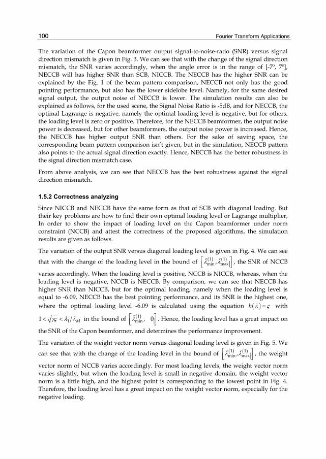
Fourier Transform Applications
100
The variation of the Capon beamformer output signal-to-noise-ratio (SNR) versus signal direction mismatch is given in Fig. 3. We can see that with the change of the signal direction mismatch, the SNR varies accordingly, when the angle error is in the range of [-7º, 7º], NECCB will has higher SNR than SCB, NICCB. The NECCB has the higher SNR can be explained by the Fig. 1 of the beam pattern comparison, NECCB not only has the good pointing performance, but also has the lower sidelobe level. Namely, for the same desired signal output, the output noise of NECCB is lower. The simulation results can also be explained as follows, for the used scene, the Signal Noise Ratio is -5dB, and for NECCB, the optimal Lagrange is negative, namely the optimal loading level is negative, but for others, the loading level is zero or positive. Therefore, for the NECCB beamformer, the output noise power is decreased, but for other beamformers, the output noise power is increased. Hence, the NECCB has higher output SNR than others. For the sake of saving space, the corresponding beam pattern comparison isn’t given, but in the simulation, NECCB pattern also points to the actual signal direction exactly. Hence, NECCB has the better robustness in the signal direction mismatch case.
From above analysis, we can see that NECCB has the best robustness against the signal direction mismatch.
1.5.2 Correctness analyzing
Since NICCB and NECCB have the same form as that of SCB with diagonal loading. But their key problems are how to find their own optimal loading level or Lagrange multiplier, In order to show the impact of loading level on the Capon beamformer under norm constraint (NCCB) and attest the correctness of the proposed algorithms, the simulation results are given as follows.
The variation of the output SNR versus diagonal loading level is given in Fig. 4. We can see
that with the change of the loading level in the bound of ( ) ( )1 1maxmin ,λ λ⎡ ⎤
⎢ ⎥⎣ ⎦, the SNR of NCCB
varies accordingly. When the loading level is positive, NCCB is NICCB, whereas, when the loading level is negative, NCCB is NECCB. By comparison, we can see that NECCB has higher SNR than NICCB, but for the optimal loading, namely when the loading level is equal to -6.09, NECCB has the best pointing performance, and its SNR is the highest one, where the optimal loading level -6.09 is calculated using the equation ( )h λ ς= with
11 Mγς λ λ< < in the bound of ( )1min , 0λ⎡ ⎤
⎢ ⎥⎣ ⎦. Hence, the loading level has a great impact on
the SNR of the Capon beamformer, and determines the performance improvement.
The variation of the weight vector norm versus diagonal loading level is given in Fig. 5. We
can see that with the change of the loading level in the bound of ( ) ( )1 1maxmin ,λ λ⎡ ⎤
⎢ ⎥⎣ ⎦, the weight
vector norm of NCCB varies accordingly. For most loading levels, the weight vector norm varies slightly, but when the loading level is small in negative domain, the weight vector norm is a little high, and the highest point is corresponding to the lowest point in Fig. 4. Therefore, the loading level has a great impact on the weight vector norm, especially for the negative loading.

Robust Beamforming and DOA Estimation
101
-40 -30 -20 -10 0 10 20 30 40 Digital Loading Level ( )λ
Beam
form
er S
NR
(dB)
6
4
2
0
-2
-4
-6
-8
Ideal-SCBSCBNCCBOptimal λ
-6.09
Fig. 4. Output SNR versus loading level
-40 -30 -20 -10 0 10 20 30 40 Digital Loading Level ( )λ
Wei
ght V
ecto
r Nor
m
1
0.9
0.8
0.7
0.6
0.5
0.4
0.3
Ideal-SCBSCBNCCBOptimal λ
-6.09
Fig. 5. Weight vector norm versus loading level
From the above simulation results, we can see that the loading level has a great impact on the performance of the Capon beamformer, and NECCB has the best pointing performance, namely, the optimal negative loading is the best. This is also consistent to the theory analysis, for the robust beamformer with diagonal loading, the improvement is determined by the optimal loading level, when the loading level is optimal, the performance
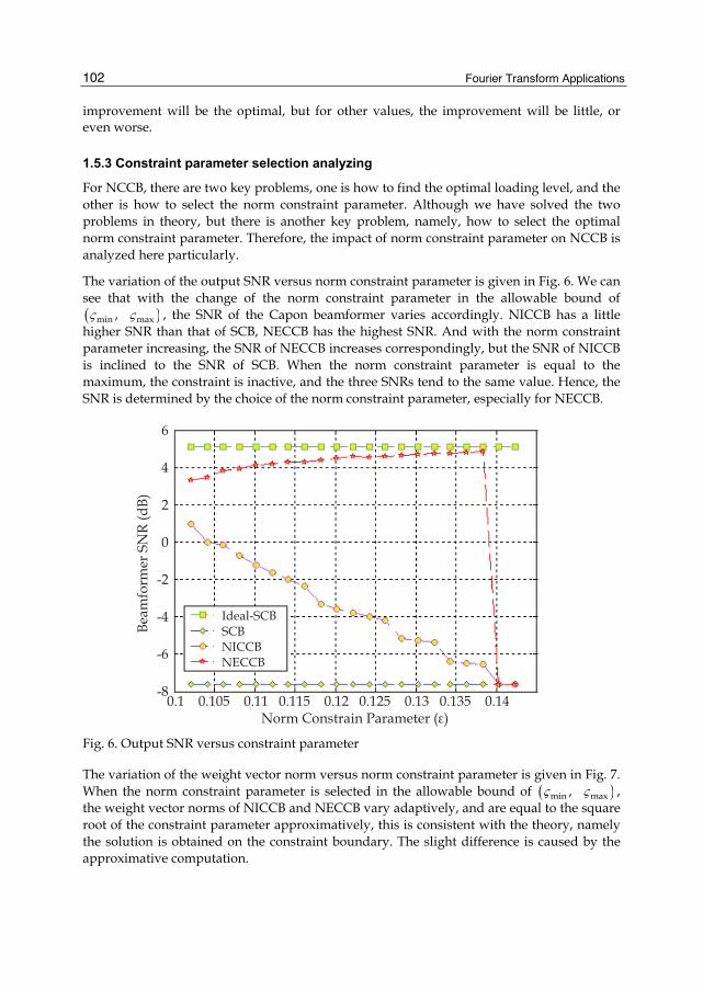
Fourier Transform Applications
102
improvement will be the optimal, but for other values, the improvement will be little, or even worse.
1.5.3 Constraint parameter selection analyzing
For NCCB, there are two key problems, one is how to find the optimal loading level, and the other is how to select the norm constraint parameter. Although we have solved the two problems in theory, but there is another key problem, namely, how to select the optimal norm constraint parameter. Therefore, the impact of norm constraint parameter on NCCB is analyzed here particularly.
The variation of the output SNR versus norm constraint parameter is given in Fig. 6. We can see that with the change of the norm constraint parameter in the allowable bound of ( )min max,ς ς , the SNR of the Capon beamformer varies accordingly. NICCB has a little higher SNR than that of SCB, NECCB has the highest SNR. And with the norm constraint parameter increasing, the SNR of NECCB increases correspondingly, but the SNR of NICCB is inclined to the SNR of SCB. When the norm constraint parameter is equal to the maximum, the constraint is inactive, and the three SNRs tend to the same value. Hence, the SNR is determined by the choice of the norm constraint parameter, especially for NECCB.
Beam
form
er S
NR
(dB)
6
4
2
0
-2
-4
-6
-8
Ideal-SCBSCBNICCBNECCB
0.1 0.105 0.11 0.115 0.12 0.125 0.13 0.135 0.14 Norm Constrain Parameter (ε)
Fig. 6. Output SNR versus constraint parameter
The variation of the weight vector norm versus norm constraint parameter is given in Fig. 7. When the norm constraint parameter is selected in the allowable bound of ( )min max,ς ς , the weight vector norms of NICCB and NECCB vary adaptively, and are equal to the square root of the constraint parameter approximatively, this is consistent with the theory, namely the solution is obtained on the constraint boundary. The slight difference is caused by the approximative computation.

Robust Beamforming and DOA Estimation
103
Wei
ght V
ecto
r Nor
m0.38
0.37
0.36
0.35
0.34
0.33
0.32
0.31
Ideal-SCBSCBNICCBNECCBNorm Contrain Value (ε)
0.1 0.105 0.11 0.115 0.12 0.125 0.13 0.135 0.14 Norm Constrain Parameter (ε)
Fig. 7. Weight norm versus constraint parameter
From above simulation results, we can see that if the norm constraint parameter is selected in the allowable bound, the norm constraint parameter has a great impact on the performance of NICCB and NECCB, especially for NECCB. But NECCB with the larger constraint parameter has the better pointing performance, namely, when the constraint parameter is selected as more larger in its allowable bound, the optimal negative loading has the optimal improvement.
1.6 Conclusion
From the above analysis, we can conclude as follows. (I) The proposed algorithm is correct and effective. (II) The norm constraint can improve the robustness of the Capon beamformer. Especially, the equality constraint has the preferable improvement to overcome the steering vector mismatch, and also has good robustness for the samples number. (III) When the norm constraint parameter is selected in the allowable bound, NECCB has the best performance, namely the optimal negative loading has the optimal improvement, this is because that the norm equality constraint is stronger than the norm inequality constraint.
2. Improved pattern synthesis method with linearly constraint minimum variance criterion Antenna pattern synthesis becomes the fundamental research contents with the wide application of the array antenna in communication, radar and other areas, and catches the attentions widely. The array antenna pattern synthesis is the task which solves the weight values of the every element to force the antenna pattern inclining to the anticipant shape. Dolph has first given the method of getting the weight function for uniform linear array to

Fourier Transform Applications
104
achieve the Chebychev pattern [39], therefore the optimal solution can be achieved in the sense of giving the mainlobe width and the maximum lowest sidelobe level. However, how to implement the pattern synthesis for the arbitrary array antenna efficiently is a challenging research task in array signal processing society.
Currently, the methods of pattern synthesis can be classified as the two types, one is the traditional vector weight methods [40-42], the other one is the matrix weight methods [43], therein, the intelligent computer methods are used to improve the calculating efficiency of the optimal weight vector, such as the genetic evolution algorithms [44] and the particle swarm optimization algorithms [45]. However, for any pattern synthesis method, the iterative operation can’t be avoided, and the iterative number determines the operation load directly, the operation load, or titled as the compute efficiency is the key metric to evaluate the validity of the pattern synthesis.
Guo Q et al propose the pattern synthesis method for the arbitrary array antenna with the linearly constraint minimun variance criterion (LCMV-PS) [45], compared with the traditional vector weight methods, this algorithm has the small iterative number and the preferable convergence. However, by analysis and simulation, it is found that the iterative coefficient determines its performance, namely, the iterative coefficient not only determines the pattern shape, but also determines the iterative number, or titled as the compute load. Therefore, how to select the iterative formula and its iterative coefficient is the key problem to reduce the compute load and enhanced the applicability.
In this chapter, for the LCMV-PS method proposed in [45], by analyzing its implementation and jammer power iterative formula, the improved fast robust LCMV-PS method is proposed [46]. This algorithm takes into account the effect of the relative amplitude between synthesis pattern and its reference upon the pattern synthesis adequately, via adding a proportion constant to the iterative formula, the effect of their relative amplitude upon the changing ratio of the jammer power is strengthened, not only the iterative efficiency of the jammer power is improved, namely the iterative number is reduced, and the pattern synthesis efficiency is improved, but also the selecting bound of the iterative coefficient is extended, namely the effect of the iterative coefficient upon the pattern synthesis is weakened, and the application area and applicability of the pattern synthesis method is enhanced greatly. The last simulation attests its correctness and effectiveness.
2.1 Pattern synthesis method with LCMV criterion
The problem of array pattern synthesis can be simplified as follows, namely for the given element number M and element position { } 1
Mi i=x , solving the complex weight vector w, and
force the array pattern ( )P θ with the definite width and maximum value in the desired direction, at the same time, make the sidelobe level according to the requirement.
The target of the pattern synthesis method for arbitrary arrays based on LCMV criterion (LCMV-PS) is making all the sidelobe peak level equal to the minimum that the array can achieve as possible. Furthermore, this method constructs many illusive jammers in the sidelobe region, and the jammer power will be justed by the synthesis pattern amplitude in its relative direction, namely, if the synthesis pattern amplitude is high in this direction, the illusive jammer power will be increased. Therefore, the LCMV-PS method can be simple described as follows:

Robust Beamforming and DOA Estimation
105
1. Specify the mainlobe region [ ]1 2,ML MLθ θ and sidelobe envelope ( )iD θ . Set the initial value of jammer power ( )0 if θ , if iθ is in the sidelobe region, ( )0 1if θ = , otherwise if in the mainlobe region, ( )0 0if θ = , 1,i N= , where N is the number of the uniformly distributed jammers with one degree spacing, namely, 1 2, , , Nθ θ θ are the degree values with the one degree spacing in the array pattern overlay region. And ( )iD θ is the given reference sidelobe envelope of the synthesis pattern.
2. Calculate jammer powers for the k-th iteration ( ) ( ) ( )1 2, , ,k k k Nf f fθ θ θ .
If k=0, then the jammer powers are the initial values ( ) ( ) ( )0 1 0 2 0, , , Nf f fθ θ θ . If k≥1, there is the iterative formula as follows:
( )[ ]
( ) ( ) ( ) [ ]
1 2
11 1 1 2
0 ,
max , 0 ,
ML ML
k k k 1k k ML ML
k 1
f P Prf Kf
Pr
θ θ θθ θ
θ θ θ θ θ− −− −
−
⎧ ∈⎪
= ⎧ ⎫−⎨ ⎪ ⎪+ ∉⎨ ⎬⎪ ⎪ ⎪⎩ ⎭⎩
(2.1)
where ( )1kf θ− is the jammer powers of the k-1-th iteration, K is the iterative coefficient. ( ) ( )1
HkP θ θ− = w a is the pattern of the k-1-th iteration, therein w is the relative weight
vector, ( )⋅a is the steering vector, and ( )H⋅ denotes the conjugate transposition. k 1Pr − is the sidelobe reference amplitude, if the arbitrary sidelobe shape is required in the pattern synthesis, it is only to substitute ( ) ( )k 1 k 1Pr θ Pr D θ− −= ⋅ for k 1Pr − in the above formula, and ( )D θ is the given sidelobe envelope.
3. Calculate the data covariance matrix xR , namely:
( ) ( ) ( )1 2, , , Hx k k k Ndiag f f fθ θ θ σ⎡ ⎤= ⋅ ⋅ +⎣ ⎦R A A I (2.2)
where ( ) ( ) ( )1 2, , , Nθ θ θ⎡ ⎤= ⎣ ⎦A a a a is the array manifold matrix. σ is a given small quantity, and I is the identity matrix, σ I is added to prevent the covariance matrix from being ill-conditioned.
4. Calculate the weight vector w according with the following LCMV beamforming algorithm, then synthesize the pattern. If it is satisfactory, stop; otherwise, go to step (2) and continue. Therein, w is solved by the below LCMV optimization problem, namely:
min
. .
H
Hs t
⎧⎪⎨⎪ =⎩
xww R w
C w f (2.3)
where C is the M×m constraint matrix, and f is the m×1 constraint value vector. Its optimal solution is:
( ) 11 1H −− −= x xw R C C R C f (2.4)
In the constraint condition of the optimization problem, the constraint of the mainlobe can be imposed, the constraint of the sidelobe can also be added, in other words, the constraint condition and parameter can be selected according to the pattern synthesis requirement.
Fourier Transform Applications
106
2.2 Improvement of the jammer power iteration formula
From the step of the LCMV-PS method, we can see that the key is the jammer power iteration in step (2), since it not only determines the synthesis pattern shape, but also determines the final iterative number.
By the particular analysis of the LCMV-PS implementing steps, it is not difficulty to find that although the relative difference of the synthesis pattern and the reference pattern
( )( )k 1 k 1 k 1P θ Pr Pr− − −− is used as the ratio factor for the gain change, and to control the change direction and quality of the jammer powers, actually, the expression of the iterative formula ( ) ( ) ( )( )( )1 1 1k k k k 1 k 1f Kf P Pr Prθ θ θ− − − − −+ − can be transformed as:
( ) ( ) ( ) ( ) ( ) ( )1 11 1 1 1k k 1 k
k k kk 1 k 1
P Pr Pf Kf f K K
Pr Prθ θ
θ θ θ− − −− − −
− −
⎛ ⎞−+ = ⋅ + −⎜ ⎟
⎝ ⎠ (2.5)
This expression indicates that the jammer powers between the adjacent iterations are different by a proportional factor, when the iterative coefficient K is given, the jammer power ratio of the adjacent iterations is determined by the relative amplitude of the synthesis pattern and the reference pattern ( )k 1 k 1P θ Pr− − . Therefore, for the given K, the change of the jammer powers in the iteration process is determined by ( )k 1 k 1P θ Pr− − , and the relationship is a linear function.
From the pattern synthesis process of the LCMV-PS method, when the synthesis pattern is higher than the reference pattern, the jammer powers should increase, and is in direct proportion to the difference of the two patterns. When the synthesis pattern is more higher than the reference pattern, the jammer powers should increase more larger. But when the synthesis pattern is close to the reference pattern, the change of the jammer power should be small, namely the adjustment should be precise at this time. Although the original iterative formula is consistent to the analyzing idea, and the change ratio of the iterative jammer powers is ( )( ) ( )1k 1 k 1K P θ Pr K− −⋅ + − , namely is in direct proportion to ( )k 1 k 1P θ Pr− − . Therefore, for the original method, K is the main parameter to determine the iterative effect and efficiency, and by the simulation, it is found that the synthesis pattern will be good when the parameter K is selected in a small region, such as the reference value K=0.1 in [42]. Actually, for the difference element number or array parameter, the optimal value of K will vary correspondingly. Hence, for the original method, how to select the optimal parameter K is the key matter, it not only determines the effect of the synthesis pattern, but also determines the efficiency of the jammer power iteration, namely the iterative number.
Since in the iterative process, it is the factor ( )( ) ( )1k 1 k 1K P θ Pr K− −⋅ + − determining the change quantity and direction of the jammer powers iteration, for the given K, the second item is constant, but the first item is the linear function of ( )k 1 k 1P θ Pr− − , and its proportional coefficient is K, namely the slope K determines the change quantity of the jammer power with ( )k 1 k 1P θ Pr− − . With the slope of the linear function increasing, namely for the given parameter Kp>1, the change ratio of ( )( ) ( )1p k 1 k 1K K P θ Pr K− −⋅ ⋅ + − with
( )k 1 k 1P θ Pr− − will be larger, namely the efficiency of the jammer power iteration will be improved. At the same time, for the given parameter Kp, when the effect of the jammer power iteration is better, the selection of K will be loosened, namely K can be selected in a wider region. Therefore, if the constant factor Kp (Kp>1) can be added as this method, the
Robust Beamforming and DOA Estimation
107
efficiency of the jammer power iteration will be improved, and the bound for selecting the iterative coefficient K will be enlarged, namely the selection of K will be simplified greatly.
Hence, in order to improve the iterative efficiency of the LCMV-PS method and simplify the selection of the iterative coefficient K, the iterative formula of the jammer power can be improved as follows, namely
( )[ ]
( ) ( )( ) [ ]
1 2
1 1 1 2
0 ,
max , 0 ,
ML ML
p k 1 k 1kk k ML ML
k 1
K P θ Prff K f
Pr
θ θ θ
θθ θ θ θ θ− −
− −−
⎧ ∈⎪
⎧ ⋅ − ⎫= ⎨ ⎪ ⎪+ ⋅ ⋅ ∉⎨ ⎬⎪⎪ ⎪⎩ ⎭⎩
(2.6)
where Kp is used to adjust the effect of the relative amplitude ( )k 1 k 1P θ Pr− − of the synthesis pattern and reference pattern upon the change ratio of the jammer power, namely is used to adjust the iterative efficiency of the pattern synthesis method, and other parameters have the same sense as forenamed. If Kp>1, the iterative efficiency will be advanced, whereas the iterative efficiency will be reduced. It is important that the effect of the iterative coefficient K upon the pattern synthesis is reduced greatly by adding the parameter Kp, therefore, the selection of parameter K will be simplified greatly.
Compared with the LCMV-PS method proposed in [42], the iterative formula of the jammer power is added by a constant Kp to adjust the iterative efficiency in this chapter, if Kp>>1, the efficiency of the proposed method will be improved greatly, therefore, the iterative number will be reduced, so that the operation load will be reduced greatly by the proposed method. At the same time, the bound for selecting K will also be enlarged greatly, and the application area and applicability of the pattern synthesis method is enhanced.
2.3 Simulations
Since the proposed method has the higher iterative efficiency and stronger applicability as compared with the LCMV-PS method proposed in [42], the simulation keystone is to compare the iterative efficiency of the two methods, and the effect of the iterative coefficient upon the two methods. The simulations are as follows.
2.3.1 Efficiency analyzing
In order to validate the efficiency of the proposed method, the single beam and multi-beam pattern synthesis examples of the uniform and non-uniform linear array are given respectively, and the single beam pattern synthesis examples of uniform and non-uniform planar array are also given respectively. For the convenience of comparison, the proposed improved LCMV-PS method is denoted as I-LCMV-PS, the LCMV-PS in [42] is denoted as LCMV-PS, the reference pattern is denoted as Reference.
The single beam synthesis pattern of the uniform linear array is given in Fig. 8. Therein, the element number is 32, the elements inter-space is half wavelength (λ/2), the mainlobe is point to 0º, the mainlobe width is 22º, the iterative parameter of jammer power K=0.5, and Kp=100. When the optimal weight vector is solved under the LCMV criterion, the mainlobe direction constraint is used only. Therein the iterative number of I-LCMV-PS is 5, but the iterative number of LCMV-PS is 20.

Fourier Transform Applications
108
0
-10
-20
-30
-40
-50
-60
-70
-80-100 -80 -60 -40 -20 0 20 40 60 80 100
Azimuth Angle (deg)
ReferenceI-LCMV-PSLCMV-PS
Beam
form
er P
atte
rn (d
B)
Fig. 8. Single beam synthesis pattern of uniform linear array
The single beam synthesis pattern of the non-uniform linear array is given in Fig. 9. Therein, the element number is 32, the element space vector is (λ/2)×[0.29595, 1.5655, 2.7845, 3.9334, 4.999, 5.9753, 6.8645, 7.6764, 8.428, 9.1413, 9.842, 10.557, 11.311, 12.127, 13.021, 14.002, 15.073, 16.226, 17.449, 18.72, 20.017, 21.312, 22.579, 23.795, 24.939, 26, 26.971, 27.856, 28.664, 29.413, 30.125, 30.825], the mainlobe is also point to 0º, the mainlobe width is also 22º, and K=0.5, Kp=100. When the optimal weight vector is solved under the LCMV criterion, the mainlobe direction constraint is used only. The iterative number of the two methods are 5 and 20, respectively.
0
-10
-20
-30
-40
-50
-60-100 -80 -60 -40 -20 0 20 40 60 80 100
Azimuth Angle (deg)
ReferenceI-LCMV-PSLCMV-PS
Beam
form
er P
atte
rn (d
B)
Fig. 9. Single beam synthesis pattern of non-uniform linear array
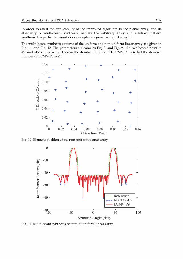
Robust Beamforming and DOA Estimation
109
In order to attest the applicability of the improved algorithm to the planar array, and its effectivity of multi-beam synthesis, namely the arbitrary array and arbitrary pattern synthesis, the particular simulation examples are given as Fig. 11.~Fig. 16.
The multi-beam synthesis patterns of the uniform and non-uniform linear array are given in Fig. 11. and Fig. 12. The parameters are same as Fig. 8. and Fig. 9., the two beams point to 45º and -45º respectively. Therein the iterative number of I-LCMV-PS is 6, but the iterative number of LCMV-PS is 25.
Y D
irec
tion
(Col
umn)
0.14
0.12
0.10
.008
0.06
0.04
0.02
0
X Direction (Row)0 0.02 0.04 0.06 0.08 0.10 0.12 0.14
Fig. 10. Element position of the non-uniform planar array
0
-10
-20
-30
-40
-50
Beam
form
er P
atte
rn (d
B)
-100 -50 0 50 100Azimuth Angle (deg)
ReferenceI-LCMV-PSLCMV-PS
Fig. 11. Multi-beam synthesis pattern of uniform linear array
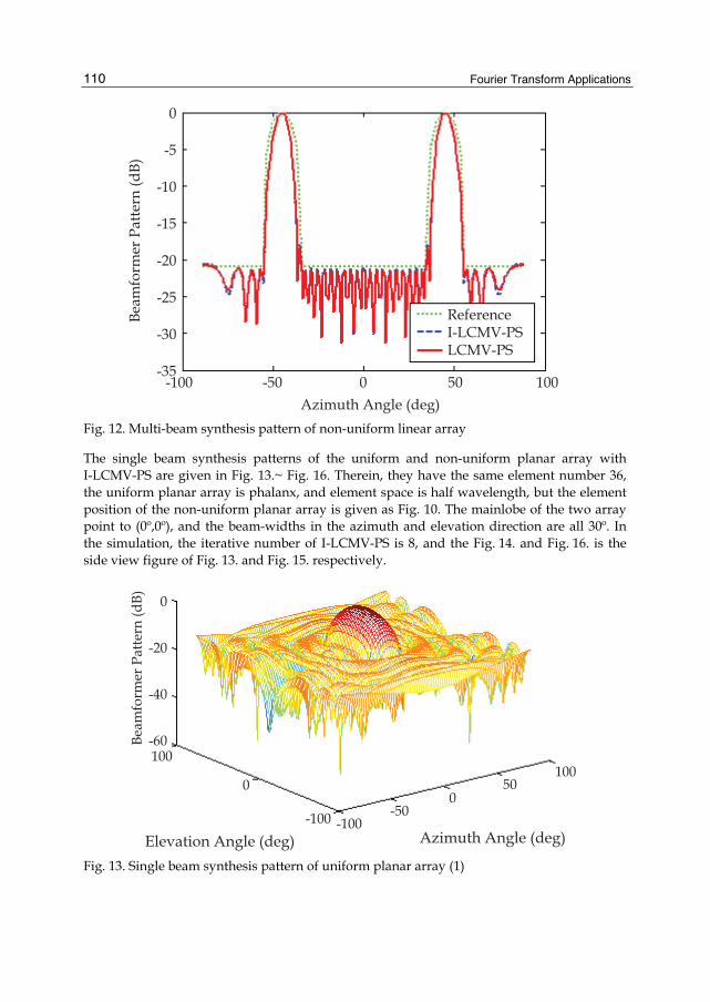
Fourier Transform Applications
110
0
-5
-10
-15
-20
-25
-30
-35
Beam
form
er P
atte
rn (d
B)
-100 -50 0 50 100Azimuth Angle (deg)
ReferenceI-LCMV-PSLCMV-PS
Fig. 12. Multi-beam synthesis pattern of non-uniform linear array
The single beam synthesis patterns of the uniform and non-uniform planar array with I-LCMV-PS are given in Fig. 13.~ Fig. 16. Therein, they have the same element number 36, the uniform planar array is phalanx, and element space is half wavelength, but the element position of the non-uniform planar array is given as Fig. 10. The mainlobe of the two array point to (0º,0º), and the beam-widths in the azimuth and elevation direction are all 30º. In the simulation, the iterative number of I-LCMV-PS is 8, and the Fig. 14. and Fig. 16. is the side view figure of Fig. 13. and Fig. 15. respectively.
Beam
form
er P
atte
rn (d
B) 0
-20
-40
-60100
0
-100Elevation Angle (deg) Azimuth Angle (deg)
-100
100
0-50
50
Fig. 13. Single beam synthesis pattern of uniform planar array (1)

Robust Beamforming and DOA Estimation
111
0
-10
-20
-30
-40
-50
-60
Beam
form
er P
atte
rn (d
B)
-100 -50 0 50 100
Fig. 14. Single beam synthesis pattern of uniform planar array (2)
Bea
mfo
rmer
Pat
tern
(dB
) 0
-10
-20
-30
-40
Elevation Angle (deg) Azimuth Angle (deg)
100
0
-100
100 50 0 -50-100
Fig. 15. Single beam synthesis pattern of non-uniform planar array (1)
From the above simulations, we can see that the two methods have the preferable synthesis pattern, but I-LCMV-PS has small iterative number, namely it has the higher pattern synthesis efficiency.

Fourier Transform Applications
112
0
-5
-10
-15
-20
-25
-30
-35
Beam
form
er P
atte
rn (d
B)
-100 -50 0 50 100 Fig. 16. Single beam synthesis pattern of non-uniform planar array (2)
2.3.2 Convergence analyzing
In order to compare the convergence characteristic, limit by the chapter length, here the example of the uniform linear array is given, about the examples of the non-uniform linear array and the planar array are similar to the uniform linear array.
Beam
form
er P
atte
rn (d
B)
0
-10
-20
-30
-40
-50
-60
-70
-80
-90-100 -80 -60 -40 -20 0 20 40 60 80 100
Azimuth angle (deg)
123≥4
Fig. 17. Synthesis pattern versus iterative number of I-LCMV-PS
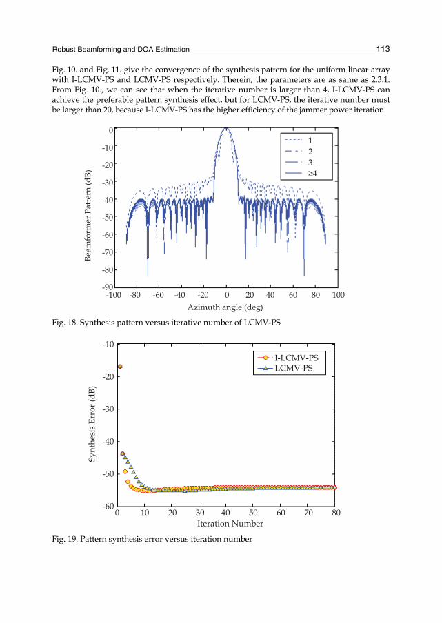
Robust Beamforming and DOA Estimation
113
Fig. 10. and Fig. 11. give the convergence of the synthesis pattern for the uniform linear array with I-LCMV-PS and LCMV-PS respectively. Therein, the parameters are as same as 2.3.1. From Fig. 10., we can see that when the iterative number is larger than 4, I-LCMV-PS can achieve the preferable pattern synthesis effect, but for LCMV-PS, the iterative number must be larger than 20, because I-LCMV-PS has the higher efficiency of the jammer power iteration.
Beam
form
er P
atte
rn (d
B)
0
-10
-20
-30
-40
-50
-60
-70
-80
-90-100 -80 -60 -40 -20 0 20 40 60 80 100
Azimuth angle (deg)
123≥4
Fig. 18. Synthesis pattern versus iterative number of LCMV-PS
-10
-20
-30
-40
-50
-60
Synt
hesi
s Er
ror (
dB)
0 10 20 30 40 50 60 70 80Iteration Number
I-LCMV-PSLCMV-PS
Fig. 19. Pattern synthesis error versus iteration number
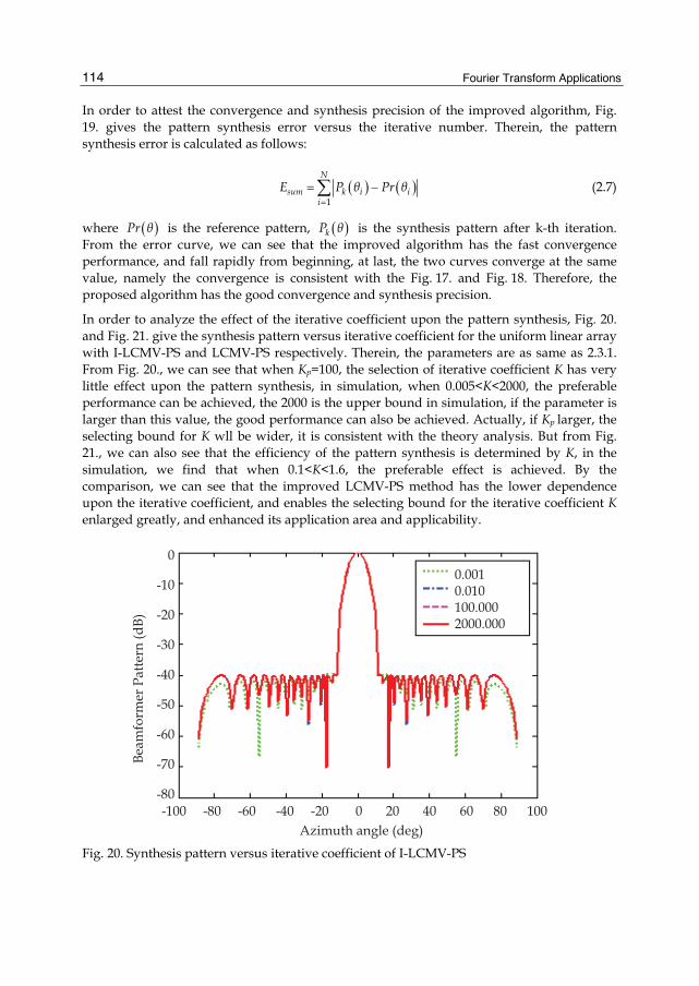
Fourier Transform Applications
114
In order to attest the convergence and synthesis precision of the improved algorithm, Fig. 19. gives the pattern synthesis error versus the iterative number. Therein, the pattern synthesis error is calculated as follows:
( ) ( )1
N
sum k i ii
E P θ Pr θ=
= −∑ (2.7)
where ( )Pr θ is the reference pattern, ( )kP θ is the synthesis pattern after k-th iteration. From the error curve, we can see that the improved algorithm has the fast convergence performance, and fall rapidly from beginning, at last, the two curves converge at the same value, namely the convergence is consistent with the Fig. 17. and Fig. 18. Therefore, the proposed algorithm has the good convergence and synthesis precision.
In order to analyze the effect of the iterative coefficient upon the pattern synthesis, Fig. 20. and Fig. 21. give the synthesis pattern versus iterative coefficient for the uniform linear array with I-LCMV-PS and LCMV-PS respectively. Therein, the parameters are as same as 2.3.1. From Fig. 20., we can see that when Kp=100, the selection of iterative coefficient K has very little effect upon the pattern synthesis, in simulation, when 0.005<K<2000, the preferable performance can be achieved, the 2000 is the upper bound in simulation, if the parameter is larger than this value, the good performance can also be achieved. Actually, if Kp larger, the selecting bound for K wll be wider, it is consistent with the theory analysis. But from Fig. 21., we can also see that the efficiency of the pattern synthesis is determined by K, in the simulation, we find that when 0.1<K<1.6, the preferable effect is achieved. By the comparison, we can see that the improved LCMV-PS method has the lower dependence upon the iterative coefficient, and enables the selecting bound for the iterative coefficient K enlarged greatly, and enhanced its application area and applicability.
Beam
form
er P
atte
rn (d
B)
0
-10
-20
-30
-40
-50
-60
-70
-80-100 -80 -60 -40 -20 0 20 40 60 80 100
Azimuth angle (deg)
0.0010.010100.0002000.000
Fig. 20. Synthesis pattern versus iterative coefficient of I-LCMV-PS

Robust Beamforming and DOA Estimation
115
Beam
form
er P
atte
rn (d
B)0
-10
-20
-30
-40
-50
-60
-70
-80-100 -80 -60 -40 -20 0 20 40 60 80 100
Azimuth angle (deg)
0.0010.1001.0002.000
Fig. 21. Synthesis pattern versus iterative coefficient of LCMV-PS
2.4 Conclusion
From the above analysis and simulation, we can conclude as follows: (I) The proposed jammer power iterative formula is correct and effective. (II) By the improvement for the iterative formula of the original method, the iterative efficiency is increased greatly, and the iterative number is reduced greatly, therefore the operation load of the pattern synthesis is reduced efficiently. (III)The improved jammer power iterative formula enlarges the selecting bound for the iterative coefficient, and reduces the effect of the parameter upon the pattern synthesis, and enhances the application area and applicability of the proposed pattern synthesis method.
3. Unitary Root-MUSIC The problem of estimating the direction-of-arrival (DOA) of narrowband sources from sensor array data has received considerable attention. The eigen-based methods for DOA estimation represent a class techniques that offer a much better resolution performance than that of conventional beamformers. In eigen-based methods, signal and noise subspaces are identified first via a M M× generalized EVD (GEVD) of the array data/noise correlation matrix pencil, where M equals the number of array elements. A search is then conducted over a null spectrum associated with the noise subspace, to locate the minima, from which the source DOA’s can be determined. In the case where a uniform linear array (ULA) is employed, the null-spectrum searching can be converted into a polynomial rooting problem. Two well known examples are the Root-MUSIC[47] and Root-Minimum-Norm[48] method. They belong to the so-called weighted root-form eigen-based methods. Compared to their spectrum-searching or spectral-form counterparts, root-form methods exhibit a higher resolution capability in dealing with closely spaced sources.Rao and Hari[49] argue that a
Fourier Transform Applications
116
zero of the null spectrum, having a large radial error, will cause the corresponding spectral minima to be less defined,but does not affect the DOA estimates. As for the mean-squared errors of the DOA estimates,Li and Vaccaro[50] show that both spectral and root-form methods yield the same expression. It should be borne in mind, however, that the result holds only when each of the sources has a minimum corresponding to it in the null spectrum.
A major issue regarding eigen-based methods is the heavy computational load associated with the GEVD. This is more significant when M is large. To remedy this the concept of beamspace transformation was proposed[51] as a means of reducing the dimension of the array data. Ta.S.L proposed a novel iterative implementation of beamspace root-form methods without the need for large-order polynomial rooting[52]. Marius.P, Alex.B.G and Martin.H proposed the unitary root MUSIC algorithm reduces the computational complexity because it exploits the eigendecomposition of a real-valued covariance matrix[53].
In this chapter [54], combining the algorithms of Root-MUSIC and Unitary-root MUSIC, the Root-MUSIC algorithm with real-valued eigendecomposition is given.
3.1 Array signal model
Assume a uniform linear array (ULA) is composed of M sensors, and let it receive q ( q M< ) narrowband signals impinging with unknown directions of arrival ((DOA)
1θ , 2θ ,… , qθ . Assume that there are N snapshots ( )1x , ( )2x ,… , ( )Nx available. The tth measured snapshot of the array is generally modeled as:
( ) ( ) ( )t t t= +x As n (3.1)
where ( ) ( )1 , , qθ θ⎡ ⎤= ⎣ ⎦A a a is the M q× composite steering matrix, the columns of which represent a basis for the signal subspace, ( )θa represents the array’s 1M × complex manifold:
( ) ( ) ( ) ( )2 sin 2 1 sin1, , ,Tj d j d Me eπ λ θ π λ θθ −⎡ ⎤= ⎢ ⎥⎣ ⎦
a (3.2)
In addition
( )ts denotes the 1q× vector of source waveforms; ( )tn denotes the 1M × vector of white sensor noise;
λ is the wavelength; d is the interelement space; ( )T⋅ denotes transpose.
It is generally assumed that signals are uncorrelated with the noise ( )tn . The sensor noise is assumed to be a zero-mean spatially and temporally uncorrelated Gaussian process with the uunknown diagonal covariance matrix given by
( ) ( ){ } { }2 2 2 2, , , ,Hn E t t diag σ σ σ σ= = =R n n I (3.3)
where {}E ⋅ is the expectation operator,and ( )H⋅ stands for the Hermitian transpose, I is the identity matrix, 2σ is the noise variance.
Robust Beamforming and DOA Estimation
117
Data model (1) allows us to write the covariance matrix of the array measurements as:
( ) ( ){ } 2H HE t t σ= = +R x x ASA I (3.4)
where ( ) ( ){ }HE t t=S s s is the q q× source waveform covariance matrix.
3.2 Root-MUSIC
Root-MUSIC is the polynomial rooting form of MUSIC, namely, the spectrum peak searching is replaced by polynomial rooting in MUSIC implementation.
In Root-MUSIC, the polynomial should be defined as follows
( ) ( ) 1, ,Hi if z z i q M= = +u a (3.5)
where, iu is the eigenvector corresponding to the M-q minimum eigen-value of the data covariance matrix, and
( ) 11 ,TMz z z −⎡ ⎤= ⎣ ⎦a (3.6)
From the above definition, we can include that the polynomial roots lie on the unit circle properly when exp( )z jω= , and ( )je ωa is the steering vector of space frequency ω. From the
eigen-space algorithms, ( )mjme ω =a a is the signal steering vector, and it is orthogonal to the
space of the noise. Therefore, the polynomial definition can be modified as the following form
( ) ( ) ( )H HN Nf z z z= a U U a (3.7)
where NU is the noise space, namely, let the eigendecomposition of the matrix R be defined in a standard way
2H H HS S S N Nσ= = +R U Λ U U Λ U U U (3.8)
where
1S q⎡ ⎤= ⎣ ⎦U u u , 1 ,N q M+⎡ ⎤= ⎣ ⎦U u u , { }1diag , ,S qλ λ=Λ and the subscripts S and N stand for signal- and noise-subspace, respectively.
Therefore, the source DOA information can be obtained when the above roots are solved. At the same time, we found the item of z∗ in the polynomial, and the solving process will become complex and difficult. In order to simplify problem, the above polynomial can be modified as
( ) ( ) ( )1 1M T HN Nf z z z z− −= a U U a (3.9)
Here, the polynomial order is 2(M-1), and has (M-1) pairs roots, the every pair roots have the mutual conjugate relationship. In the (M-1) pairs roots, there are q roots 1 , , qz z are distributed on the unit circle, and

Fourier Transform Applications
118
( )exp , 1i iz j i qω= ≤ ≤ (3.10)
For the ULA, the corresponding DOA of signal can be calculated as
( )arcsin arg , 1, ,2i iz i q
dλθπ
⎛ ⎞= =⎜ ⎟⎝ ⎠
(3.11)
where λ is the signal wavelength, d is the array space.
A simple alternative method is proposed in Ref.[55]. From above analysis, we can see that the signal space is orthogonal to the noise space, therefore
exp 2 sin , 1, ,i idz j i qπ θλ
⎛ ⎞= =⎜ ⎟⎝ ⎠
(3.12)
should be q roots of all M-q polynomials in Eq. (3.9), namely
( ) 0, 1, , , 1, ,i jf z j q i q M= = = + (3.13)
Eq.(3.9) represents M-q polynomials of M-1 order. From Eq.( 3-13), they should have a q-order maximum common factor, which can be denoted as ( )f z . The DOAs of all the sources can be obtained by rooting ( )f z . From the eigenvectors of the noise space, ( )f z can be obtained as follows
There exists a vector 1T
M qb b −⎡ ⎤= ⎣ ⎦b which satisfies
11 1
2
1 0 0H TNH
N qH MN
c c×
⎡ ⎤⎡ ⎤= =⎢ ⎥ ⎣ ⎦⎢ ⎥⎣ ⎦
UU b b
U (3.14)
where 1NU is q×(M-q) sub-matrix and 2NU is (M-q)×(M-q) sub-matrix of NU . This can be understood by noticing that the product of NU and b represents a linear combination of noise vectors represented in the M-q dimensional noise space. The product 2NU and b defines a system of M-q equations with M-q unknowns. b can be fixed to be the solution that results in a product [ ]1 0 T . The product of 1NU and b is then a set of coefficients that are determined.
Adopting this approach b is obtained by
[ ] ( )12 11 0 0 T
N M q−
× −=b U (3.15)
And 1 qc c⎡ ⎤= ⎣ ⎦c is determined easily as
[ ] ( )1
1 1 2 11 0 0 TN N N M q
−× −
= =c U b U U (3.16)
Now that c has been determined, the polynomial ( )f z is formed by
( )1
11
1, 1
qi
i Mi
f z c z c+
−+
== =∑ (3.17)

Robust Beamforming and DOA Estimation
119
Eq.(3.17) has q roots which are correspond to the DOAs of q sources. After obtaining q roots of Eq.(3.13), { } 1
qi iz
=, the DOAs of the sources are obtained by Eq.(3.12).
From the well known conventional Root-MUSIC polynomial of Eq.(3.7), we can conclude that it is a function of z, namely
( ) ( ) ( ) ( ){ } ( )1 1Root MUSIC 1 1 1M T H M T H
N N S Sf z z z z z z z− −− = = −a U U a a U U a (3.18)
Here the orthogonal property of the signal and noise subspace is used.
3.3 Root-MUSIC with real-valued eigendecomposition
The matrix R is the centro-Hermitian if
∗=R JR J (3.19)
where J is the exchange matrix with ones on its antidiagonal and zeros elsewhere, and ( )∗⋅ stands for complex conjugate. The matrix (3.3)is known to be centro-Hermitian if and only if S is a diagonal matrix, i.e., when the signal source are uncorrelated. However, to ‘double’ the number of snapshots and decorrelate possibly correlated source pairs in the case of an arbitrary matrix S , the centro-Hermitian property is sometimes forced by means of the so-called forward-backward (FB) averaging:
( )~
212
HFB σ∗= + = +R R JR J ASA I (3.20)
where
( )~ 1
2∗= +S S DS D (3.21)
( ) ( ) ( ) ( ){ }1 2 1 sin2 1 sin , , ,qj d Mj d Mdiag e e π λ θπ λ θ − −− −=D (3.22)
Let us define the matrix as:
= HFBC Q R Q (3.23)
therefore, the C is a real-valued covariance matrix, where Q is any unitary,column conjugate symmetric M M× matrix. Any matrix Q is column conjugate symmetric if
∗ =JQ Q (3.24)
For example, the following sparse matrices
212n
jj
⎡ ⎤= ⎢ ⎥−⎣ ⎦
I IQ
J J (3.25)
2 11 22
T Tn
j
j+
⎡ ⎤⎢ ⎥
= ⎢ ⎥⎢ ⎥−⎣ ⎦
I 0 I
Q 0 0J 0 J
(3.26)

Fourier Transform Applications
120
can be chosen for arrays with an even and odd number of sensors,respectively, where the vector ( )0, 0, , 0 T=0
From (3.23), and insert (3.20) to it, it follows that
( ) ( )1 12 2
∗ ∗⎡ ⎤ ⎡ ⎤= = + = +⎢ ⎥ ⎣ ⎦⎣ ⎦H H H H
FBC Q R Q Q R JR J Q Q RQ Q JR J Q (3.27)
using ∗ =JQ Q , ∗ =Q JQ and H =J J , we obtain that
( ) ( )
( ) ( ) ( )
1 12 21 12 2Re
∗ ∗
∗∗ ∗ ∗
⎡ ⎤⎡ ⎤= + = +⎣ ⎦ ⎣ ⎦
⎡ ⎤ ⎡ ⎤= + = +⎢ ⎥ ⎢ ⎥⎣ ⎦ ⎣ ⎦⎡ ⎤= ⎣ ⎦
HH H H
HH H H
H
C Q RQ Q JR JQ Q RQ JQ R JQ
Q RQ Q R Q Q RQ Q RQ
Q RQ
(3.28)
therefore, we prove that C is a real-valued covariance matrix.
Let the eigendecompositions of the matrices R , FBR and C be defined in a standard way
2H H HS S S N Nσ= = +R V Π V V Π V V V (3.29)
2H H HFB S S S N Nσ= = +R U Λ U U Λ U U U (3.30)
2H H HS S S N NC σ= = +E Γ E E Γ E E E (3.31)
where
1 , ,S q⎡ ⎤= ⎣ ⎦V v v , 1 , ,N q M+⎡ ⎤= ⎣ ⎦V v v , { }1 , ,S qdiag π π=Π
1 , ,S q⎡ ⎤= ⎣ ⎦U u u , 1 , ,N q M+⎡ ⎤= ⎣ ⎦U u u , { }1 , ,S qdiag λ λ=Λ
1 , ,S q⎡ ⎤= ⎣ ⎦E e e , 1 , ,N q M+⎡ ⎤= ⎣ ⎦E e e , { }1 , ,S qdiag γ γ=Γ
and the subscripts S and N stand for signal- and noise-subspace,respectively.
Assume the Characteristic equation for the matrix FBR as
λ⋅ = ⋅FBR u u (3.32)
we can obtain that
H H Hλ λ⋅ = ⋅ = ⋅FBQ R u Q u Q u (3.33)
with the use of equation: =HQQ I and the definition of C ,we obtain that
H H Hλ⋅ = ⋅ ⋅ ⋅ = ⋅ = ⋅H HFB FBQ R u Q R QQ u C Q u Q u (3.34)
Equation Hλ⋅ = ⋅HC Q u Q u can be identified as the characteristic one for the real-valued covariance matrix C .

Robust Beamforming and DOA Estimation
121
Hence, using (3.30), (3.31), (3.32) and (3.34), the eigenvectors and eigenvalues of the matrices FBR and C are related as
H=E Q U (3.35)
=Γ Λ (3.36)
It is well known that the conventional Root-MUSIC polynomial is given by
( ) ( ) ( )1T HMUSIC N Nf z z z= a V V a (3.37)
( ){ } ( )1 1T HS Sz z= −a V V a (3.38)
where
( ) 11, , ,TMz z z −⎡ ⎤= ⎣ ⎦a (3.39)
jz e ω= , and ( )2 sindω π λ θ= . Similarly to(3.37) and (3.38), the FB root-MUSIC polynomial can be used:
( ) ( ) ( )1 1M T HFB MUSIC N Nf z z z z−
− = a U U a (3.40)
( ){ } ( )1 1 1M T HS Sz z z−= −a U U a (3.41)
A simple manipulation with the use of (3.35) and =HQQ I , we can obtain that:
( ) ( ) ( )1 1M T HFB MUSIC N Nf z z z z−
− = ⋅ ⋅ ⋅ ⋅H Ha QQ U U QQ a (3.42)
( ) ( ) ( ) ( )1 1M TN Nz z z−= ⋅ ⋅ ⋅ ⋅
HH H Ha Q Q U Q U Q a (3.43)
( ) ( )1 1M T HN Nz z z−= ⋅ ⋅ ⋅ ⋅ ⋅Ha Q E E Q a (3.44)
( ) ( )~ ~
1 1T
M HN Nz z z−= ⋅ ⋅ ⋅a E E a (3.45)
( )C MUSICf z−= (3.46)
where the manifold
( ) ( )~
z z= ⋅Ha Q a (3.47)
should be exploited for the polynomial rooting in (3.45). The relationship between the former and the new manifolds follows from the expression for the real-valued covariance matrix (3.23). From (3.23)and (3.20), we have
Fourier Transform Applications
122
~ ~2 2
~ ~ ~2
H H
H
σ σ
σ
⎛ ⎞= = + = +⎜ ⎟
⎝ ⎠
= +
H H H HFB
H
C Q R Q Q ASA I Q Q ASA Q Q Q
ASA Q Q
(3.48)
(3.49)
where
~
H=A A Q (3.50)
Let us term the polynomial (3.46) as the polynomial of Root-MUSIC with real-valued eigendecomposition (RVED-Root-MUSIC), since it exploits the eigendecomposition of the real-valued matrix (3.24) instead of that of the complex matrices (3.18) or (3.20). But from (3.42) to (3.44), it is clear that the FB and RVED-Root-MUSIC polynomials are identical. Hence, the performance of RVED-ROOT-MUSIC does not depend on a particular choice of the unitary column conjugate symmetric matrix Q .
3.4 Polynomial coefficient finding
From (3.44) and (3.45), we obtain the polynomial of RVED-Root-MUSIC, which is a function of z . The next thing is finding the coefficient of the polynomial[56]..
Using (3.44), we have:
( ) ( ) ( )
( ) ( )
1
1
1
1
M T HC MUSIC N N
M T
f z z z z
z z z
−−
−
= ⋅ ⋅ ⋅ ⋅ ⋅
= ⋅ ⋅
Ha Q E E Q a
a G a (3.51)
where
( ),H
N N i j M Mg
×= ⋅ ⋅ ⋅ =HG Q E E Q (3.52)
Inserting (3.39) into (3.52), and with simple manipulation, we obtain that
( ) ( ) ( )
( )
( )
1 11 1 1
1,1 1,11 2 1
,1 ,
1
,1 ,2 ,1 1 1
1
, 1
1, , , 1, , ,
, , , 1 1, , ,
1
, , ,
1
TM MMC MUSIC
M TMM M
M M M
M M MM i M i M i
i i i Mi i i
M
Mi
f z z z z z z
g gz z z z
g g
zg z g z g z
z
g z
− − −− −−
−− −
− − −
= = =−
−
⎡ ⎤ ⎡ ⎤= ⋅ ⋅⎣ ⎦ ⎣ ⎦
⎡ ⎤⎢ ⎥ ⎡ ⎤⎡ ⎤= ⋅ ⋅⎢ ⎥⎣ ⎦ ⎣ ⎦⎢ ⎥⎣ ⎦
⎡ ⎤⎢ ⎥
⎡ ⎤ ⎢ ⎥= ⋅⎢ ⎥ ⎢ ⎥⎣ ⎦ ⎢ ⎥
⎢ ⎥⎣ ⎦
= ⋅
∑ ∑ ∑
G
( )11,2 ,
1 1 1
M M MMi M i M i
i i Mi i i
z g z z g z−− −
= = =
⎛ ⎞ ⎛ ⎞ ⎛ ⎞+ ⋅ + + ⋅⎜ ⎟ ⎜ ⎟ ⎜ ⎟
⎝ ⎠ ⎝ ⎠ ⎝ ⎠∑ ∑ ∑
Robust Beamforming and DOA Estimation
123
the polynomial of RVED-Root-MUSIC is given by
( ) ( )( )( )
( ) ( )
( )( ) ( )
( )
2 2 01,
2 2 12, 2, 1
2 2 23, 2, 1 1, 2
2 2 1, 1, 1 2,2 1,1
2 2, 1 1, 2 3,2 2,1
2 2 1, 1 1, 2 3,2 2,1
2,2 1,1
MC MUSIC M
MM M
MM M M
M MM M M M
M MM M M M
M MM M M M
MM M
f z g z
g g z
g g g z
g g g g z
g g g g z
g g g g z
g g z
− −−
− −−
− −− −
− − −− −
− −− − −
− − +− − −
−−
= ⋅
+ + ⋅
+ + + ⋅
+
+ + + + + ⋅
+ + + + + ⋅
+ + + + + ⋅
+
+ + ⋅ ( )
( ) ( )
2 3
2 2 2,1
M M
M M MMg z
− + −
− − + −+ ⋅
So the number of coefficient of the polynomial is 2 1M − , and the computation of the coefficient is given as follows
( )
,1
2 1 1
,1
1, 2, ,
1, 2, , 2 1
k
i M k ii
kM k
k M i ii
g k L
a
g k L L L
− +=
− − +
− +=
⎧⎪ =⎪⎪= ⎨⎪⎪ = + + −⎪⎩
∑
∑
(3.53)
where ka denotes the kth coefficient of the polynomial.
Based upon our analysis, using (3.4), (3.20), (3.23), (3.35), (3.26), (3.31), (3.35), (3.44), (3.51), (3.52) and (3.53), the fast algorithm for RVED-Root-MUSIC can be formulated as the following seven-step procedure:
Step 1. Compute R and FBR with the use of (3.4) and (3.6).and the estimate is given by
( ) ( )1
1 NH
kk k
N
∧
== ∑R x x then 1
2FB
∗∧ ∧ ∧⎛ ⎞⎜ ⎟= +⎜ ⎟⎝ ⎠
R R JR J .
Step 2. Compute C , and the Q is dependent on the number of array sensors. The estimate
of the real-valued covariance matrix is given by ∧ ∧= H
FBC Q R Q
Step 3. Obtain NE from the eigendecomposition of C .and the estimate of NE , ∧E is given
by the eigendecomposition of ∧C
Step 4. Compute G with the use of (3.52). And the estimate of G , ∧G is given by
H
N N∧ ∧
= ⋅ ⋅ ⋅ HG Q E E Q

Fourier Transform Applications
124
Step 5. Compute the coefficient of the polynomial by (3.53). Step 6. Find the root of the polynomial (3.51), and select the q roots that are nearest to the
unit circle as being the roots corresponding to the DOA estimates. Step 7. DOA estimate, using:
( )arcsin arg 1, ,2k kz k q
dλθπ
⎛ ⎞= =⎜ ⎟⎝ ⎠
where kz represents one of the q roots selected for DOA estimation.
From the above analysis, we can conclude that the RVED-Root-MUSIC has a lower computational complexity than the conventional root-MUSIC technique thanks to the eigendecomposition of the real-valued matrix instead of that of the complex matrices, and the asymptotic performance of it is better than of conventional root-MUSIC due to the FB averaging effect..
3.5 Simulations
In this section, we present some simulation results to illustrate the performance of RVED-Root-MUSIC. We consider a ULA with M=8 elements and the inter-element space is equal to a half of wavelength. There are three signals with SNRs of 30 dB impinges on the array from 1 80θ = − , 2 20θ = − , 3 40θ = . The detailed simulation results are shown as Fig. 22. ~ Fig. 25.
0.35
0.30
0.25
0.20
0.15
0.10
0.05
0
DO
A D
epar
ture
RVED Root MUSIC
-80-20 40
0 200 400 600 800 1000Snapshot Number
Fig. 22. DOA departure vs dnapshot number. Signal DOA=[-80 -20 40], SNR=5dB
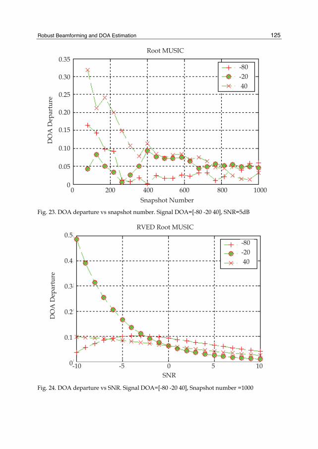
Robust Beamforming and DOA Estimation
125
0.35
0.30
0.25
0.20
0.15
0.10
0.05
0
DO
A D
epar
ture
Root MUSIC
-80-20 40
0 200 400 600 800 1000Snapshot Number
Fig. 23. DOA departure vs snapshot number. Signal DOA=[-80 -20 40], SNR=5dB
0.5
0.4
0.3
0.2
0.1
0
DO
A D
epar
ture
RVED Root MUSIC
-80-20 40
-10 -5 0 5 10SNR
Fig. 24. DOA departure vs SNR. Signal DOA=[-80 -20 40], Snapshot number =1000
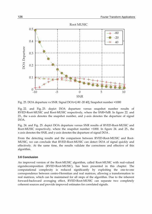
Fourier Transform Applications
126
0.5
0.4
0.3
0.2
0.1
0
DO
A D
epar
ture
Root MUSIC
-80-20 40
-10 -5 0 5 10SNR
Fig. 25. DOA departure vs SNR. Signal DOA=[-80 -20 40], Snapshot number =1000
Fig. 22. and Fig. 23. depict DOA departure versus snapshot number results of RVED-Root-MUSIC and Root-MUSIC respectively, where the SNR=5dB. In figure 22. and 23., the x-axis denotes the snapshot number, and y-axis denotes the departure of signal DOA.
Fig. 24. and Fig. 25. depict DOA departure versus SNR results of RVED-Root-MUSIC and Root-MUSIC respectively, where the snapshot number =1000. In figure 24. and 25., the x-axis denotes the SNR, and y-axis denotes the departure of signal DOA .
From the detecting results and the comparison between RVED-Root-MUSIC and Root-MUSIC, we can conclude that RVED-Root-MUSIC can detect DOA of signal quickly and effectively. At the same time, the results validate the correctness and effective of this algorithm.
3.6 Conclusion
An improved version of the Root-MUSIC algorithm, called Root-MUSIC with real-valued eigendecomposition (RVED-Root-MUSIC), has been presented in this chapter. The computational complexity is reduced significantly by exploiting the one-to-one correspondence between centro-Hermitian and real matrices, allowing a transformation to real matrices, which can be maintained for all steps of the algorithm. Due to the inherent forward-backward averaging effect, RVED-Root-MUSIC can separate two completely coherent sources and provide improved estimates for correlated signals.
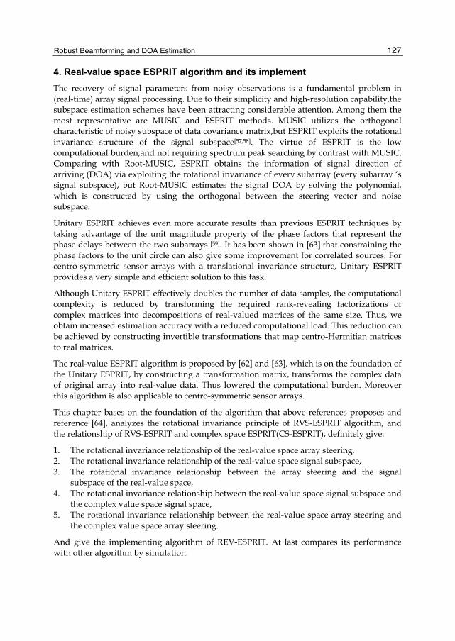
Robust Beamforming and DOA Estimation
127
4. Real-value space ESPRIT algorithm and its implement The recovery of signal parameters from noisy observations is a fundamental problem in (real-time) array signal processing. Due to their simplicity and high-resolution capability,the subspace estimation schemes have been attracting considerable attention. Among them the most representative are MUSIC and ESPRIT methods. MUSIC utilizes the orthogonal characteristic of noisy subspace of data covariance matrix,but ESPRIT exploits the rotational invariance structure of the signal subspace[57,58]. The virtue of ESPRIT is the low computational burden,and not requiring spectrum peak searching by contrast with MUSIC. Comparing with Root-MUSIC, ESPRIT obtains the information of signal direction of arriving (DOA) via exploiting the rotational invariance of every subarray (every subarray ‘s signal subspace), but Root-MUSIC estimates the signal DOA by solving the polynomial, which is constructed by using the orthogonal between the steering vector and noise subspace.
Unitary ESPRIT achieves even more accurate results than previous ESPRIT techniques by taking advantage of the unit magnitude property of the phase factors that represent the phase delays between the two subarrays [59]. It has been shown in [63] that constraining the phase factors to the unit circle can also give some improvement for correlated sources. For centro-symmetric sensor arrays with a translational invariance structure, Unitary ESPRIT provides a very simple and efficient solution to this task.
Although Unitary ESPRIT effectively doubles the number of data samples, the computational complexity is reduced by transforming the required rank-revealing factorizations of complex matrices into decompositions of real-valued matrices of the same size. Thus, we obtain increased estimation accuracy with a reduced computational load. This reduction can be achieved by constructing invertible transformations that map centro-Hermitian matrices to real matrices.
The real-value ESPRIT algorithm is proposed by [62] and [63], which is on the foundation of the Unitary ESPRIT, by constructing a transformation matrix, transforms the complex data of original array into real-value data. Thus lowered the computational burden. Moreover this algorithm is also applicable to centro-symmetric sensor arrays.
This chapter bases on the foundation of the algorithm that above references proposes and reference [64], analyzes the rotational invariance principle of RVS-ESPRIT algorithm, and the relationship of RVS-ESPRIT and complex space ESPRIT(CS-ESPRIT), definitely give:
1. The rotational invariance relationship of the real-value space array steering, 2. The rotational invariance relationship of the real-value space signal subspace, 3. The rotational invariance relationship between the array steering and the signal
subspace of the real-value space, 4. The rotational invariance relationship between the real-value space signal subspace and
the complex value space signal space, 5. The rotational invariance relationship between the real-value space array steering and
the complex value space array steering.
And give the implementing algorithm of REV-ESPRIT. At last compares its performance with other algorithm by simulation.

Fourier Transform Applications
128
This chapter is organized as follows[65]. It starts with a review of the signal model and the rotational invariance subspace principle. Next the RVS-ESPRIT algorithm is analyzed, among which includes the transformation from the complex space to real-value space, the rotational invariance principle of real-value space, and its implementing algorithm. Finally, the computer simulations with the comparison the performance of RVS-ESPRIT and the well-known LS- ESPRIT algorithm are given.
4.1 Signal model
Assume that there are two completely same subarray, their space Δ is already known, and every subarray consists of m elements. Consider N ( )N m< narrowband plane waves from far-field of the array, these plane waves are assumed to be impinging on the array from directions 1 2, , , Nθ θ θ , among them, iθ , 1, 2, ,i N= is angle between the array normal and the direction of the ith signal of the N narrowband planes waves imping. Because the structure of two arrays is completely same, therefore, for a signal, the difference of the two subarray outputs is only one phase difference iϕ , 1, 2, ,i N= . Suppose the first subarray receives the data for 1X , the second receives the data for 2X , then:
( ) ( )1 1 1 1Nθ θ⎡ ⎤= + = ⋅ +⎣ ⎦X a a S N A S N (4.1)
( ) ( )12 1 2 2
Nj jNe eϕ ϕθ θ⎡ ⎤= + = ⋅ +⎣ ⎦X a a S N AΦ S N (4.2)
Where, the direction matrix of subarray 1 is ( ) ( )1 1 Nθ θ⎡ ⎤= = ⎣ ⎦A A a a , the direction matrix of subarray 2 is 2 =A AΦ , S is the space signal vector, 1N and 2N are the noise vectors of the subarray 1 and 2, respectively,and are assumed to be white Gaussian, and among the formula:
1 Nj jdiag e eϕ ϕ⎡ ⎤= ⎣ ⎦Φ (4.3)
4.2 The rotational invariance subspace principle
From the above mathematics model, we can know that the signal direction information is included in A and Φ , because Φ is a diagonal matrix, so that we can obtain the DOA of signal through solving Φ , that is:
2 sin k
kπ Δ θ
ϕλ
⋅= (4.4)
where λ is the center wave-length of Arriving the wave. So if we obtain the rotational invariance relationship Φ of the two subarray, we can get the signal DOA information. First uniting the two subarray models, namely:
1 1
2 2
⎡ ⎤ ⎡ ⎤ ⎡ ⎤= = + = ⋅ +⎢ ⎥ ⎢ ⎥ ⎢ ⎥⋅⎣ ⎦ ⎣ ⎦ ⎣ ⎦
X A NX S A S N
X A Φ N (4.5)
Under the ideal condition, the covariance matrix is estimated as fellows:

Robust Beamforming and DOA Estimation
129
{ } HHS NE= ⋅ = ⋅ ⋅ +R X X A R A R (4.6)
where { }HS E= ⋅R S S , { }H
N E= ⋅R N N .
Let the eigendecompositions of the covariance matrix, there is:
2
1
mH H H
i i i S S S N N Ni
e eλ=
= = ⋅ ⋅ + ⋅ ⋅∑R U Σ U U Σ U (4.7)
Very obviously, the eigenvalue that gets from the top have the relationship as follows: 1 1 2N N mλ λ λ λ+≥ ≥ > = = . where SU is signal subspace that spanned by eigenvectors
which are corresponding to large eigenvalues, NU is noise subspace that spanned by eigenvectors which are corresponding to small eigenvalues.
We know that the signal subspace is spanned by large eigenvector is equal to that is spanned by array direction matrix in the above eigendecomposition, that is:
{ } ( ){ }Sspan span θ=U A (4.8)
At this time, existing a nonsingular matrix T , which can make:
( )S θ= ⋅U A T (4.9)
Obviously above-mentioned structure is coming into existence to the two subarrays, so have:
1
2
SS
S
⋅⎡ ⎤ ⎡ ⎤= =⎢ ⎥ ⎢ ⎥⋅⎣ ⎦ ⎣ ⎦
U A TU
U AΦ T (4.10)
Very obvious, the subspace spanned by array direction matrix A is equal to 1SU and 2SU which are spanned by the large eigenvectors of subarray 1 and 2 respectively.
{ } ( ){ } { }1 2S Sspan span spanθ= =U A U (4.11)
Moreover, from the relationship of the two subarrays with regard to signal direction matrix, we can know:
2 1=A A Φ (4.12)
Again from (4.10),we can know:
1
1 11
2 2 1
S S
S S S
−
−
⎧= ⋅ = ⋅⎧ ⎪⇒⎨ ⎨= ⋅ = ⋅ = ⋅ ⋅ ⋅⎩ ⎪⎩
U A T A U TU AΦ T U AΦ T U T Φ T
(4.13)
12 1 1S S S
−= ⋅ ⋅ ⋅ = ⋅U U T Φ T U Ψ (4.14)
where 1−= ⋅ ⋅Ψ T Φ T . (4.12) reflects the rotational invariance characteristic of the signal direction matrix of the two subarrays, but (4.14) reflects the rotational invariance characteristic of the received signal data subspace of the two subarrays.

Fourier Transform Applications
130
If the signal direction matrix A is full rank, we can obtain form (4.14) as fellows:
1−= ⋅ ⋅Φ T Ψ T (4.15)
So that,the diagonal matrix which is consisted of the eigenvalues of Ψ certainly be equal to Φ , but the every column of T is the eigenvectors of Ψ . Therefore, once we get the rotational invariance matrix Ψ , we can obtain the signal DOA from (4.4) directly.
4.3 Real-value space ESPRIT algorithm
4.3.1 The transformation from complex space into realvalue space
We know that the uniform linear array is centro-symmetric, and its signal direction matrix satisfy the nether formula:
M∗⋅ = ⋅J A A Δ (4.16)
where, MJ is the M M× exchange matrix with ones on its antidiagonal and zeros elsewhere, and the signal direction matrix makes reference to the first element of the array, the diagonal matrix ( )1M− −=Δ Φ , and the Φ is expressed as (4.3). If the reference point is selected as the central point of the array, so we have:
( ) ( )1 21C C C Nβ β⎡ ⎤= ⋅ = ⎣ ⎦A A Δ a a (4.17)
where
( ) ( ) ( )1 1
12 21i i
ii
M Mj jTj MjC i ie e e e
β ββββ β− −⎛ ⎞ ⎛ ⎞− −⎜ ⎟ ⎜ ⎟− −−⎝ ⎠ ⎝ ⎠⎡ ⎤= =
⎣ ⎦a a (4.18)
If matrix Q satisfying:
M∗⋅ =J Q Q (4.19)
we call it as the left real transformation matrix.
For example, Q can be chosen for arrays with an even and odd number of sensors respectively as the following sparse matrices:
212
n nn
n n
jj
⎡ ⎤= ⎢ ⎥−⎣ ⎦
I IQ
J J (4.20)
2 11 22
n nT T
n
n n
j
j+
⎡ ⎤⎢ ⎥
= ⎢ ⎥⎢ ⎥−⎣ ⎦
I 0 I
Q 0 0J 0 J
(4.21)
Moreover, from the bidirectional averaging algorithm, we can process the array data by once bidirectional averaging, and insert (4.16) into it, we can obtain:
( )12FB M M
∗= + ⋅ ⋅R R J R J (4.22)

Robust Beamforming and DOA Estimation
131
Insert HS N= ⋅ ⋅ +R A R A R into(4.13), we can obtain:
( )
( )
1212
H HFB S N M S N M
H TS N M S M M N M
∗
∗ ∗ ∗
⎛ ⎞= ⋅ ⋅ + + ⋅ ⋅ ⋅ + ⋅⎜ ⎟⎝ ⎠
= ⋅ ⋅ + + ⋅ ⋅ ⋅ ⋅ + ⋅ ⋅
R A R A R J A R A R J
A R A R J A R A J J R J (4.23)
because of ( ) ( )H H T H H
M M M∗ ∗⋅ = ⋅ ⇒ ⋅ = ⋅ ⇒ ⋅ = ⋅J A A Δ J A A Δ A J Δ A , and insert it into
(4.23), get the result:
( ) ( )( ) '
1 12 212
12
H HFB S S N M N M
H HS S N
H
L
∗ ∗
∗
= ⋅ + ⋅ ⋅ ⋅ + + ⋅ ⋅
= ⋅ + ⋅ ⋅ ⋅ +
= ⋅
R A R Δ R Δ A R J R J
A R Δ R Δ A R
Z Z
( )
( )
4.24
4.25
where
M L∗⎡ ⎤= ⋅ ⋅⎣ ⎦Z X J X J (4.26)
Since:
( )( )
( )
( ) ( )
1 12 2
121
21
2
1 1 12
HHM L M L
H H T HM L L M
H T HM M
H H HM M
H H HM M
L L
L
L
L
L L
∗ ∗
∗
∗
∗
∗
⎡ ⎤ ⎡ ⎤⋅ = ⋅ ⋅ ⋅ ⋅ ⋅⎣ ⎦ ⎣ ⎦
= + ⋅ ⋅ ⋅ ⋅ ⋅
= + ⋅ ⋅ ⋅
⎛ ⎞= + ⋅ ⋅⎜ ⎟⎝ ⎠⎡ ⎤⎛ ⎞= ⋅ + ⋅ ⋅ ⋅⎢ ⎥⎜ ⎟
⎝ ⎠⎢ ⎥⎣ ⎦
Z Z X J X J X J X J
XX J X J J X J
XX J X X J
XX J XX J
X X J X X J
(4.27)
Because ( )1 H
L
∧= ⋅R X X is the estimating formula of R . Thus (4.25) is established. When the
row number of data vector X is odd, we can definite:
1
2
T
M L×
⎡ ⎤⎢ ⎥
= ⎢ ⎥⎢ ⎥⎣ ⎦
X
X xX
(4.28)
If we process Z which is defined by (4.26) By means of matrix Q which is defined by (4.20) or (4.21) as fellows:
( ) 2HM L= ⋅ ⋅T X Q Z Q

Fourier Transform Applications
132
( )
{ } { }{ } { }
{ } { }
2
1 2 1 2
1 2 1 2
Re Im
2 Re 2 Im
Im Re
HM L
T T
∗ ∗
∗ ∗
= ⋅ ⋅
⎡ ⎤+ − −⎢ ⎥⎢ ⎥= −⎢ ⎥⎢ ⎥
+ −⎢ ⎥⎣ ⎦
T X Q Z Q
X JX X JX
x x
X JX X JX
(4.29)
If the row dimension of the data vector is even, the transformation matrix is:
( )
{ } { }{ } { }
2
1 2 1 2
1 2 1 2
Re Im
Im Re
HM L
∗ ∗
∗ ∗
= ⋅ ⋅
⎡ ⎤+ − −⎢ ⎥= ⎢ ⎥+ −⎢ ⎥⎣ ⎦
T X Q Z Q
X JX X JX
X JX X JX
(4.30)
What to need to be noticed here is, the matrix Q which defined by (4.20) and (4.21) satisfies
H⋅ =Q Q I (4.31)
From the transformation relationship of (4.28) and (4.29), we can see that ( )T X transforms complex data into real data, so that the computational burden is lowered greatly, and we can obtain:
( ) ( )
( )( )
2 2 2 2
121 1
2 21 1
2 2
HT
HH H H H HM L M L M L L M
H H H HM M M M
HM FB M
L
L L
L L
= ⋅
= ⋅ ⋅ ⋅ ⋅ ⋅ = ⋅ ⋅ ⋅ ⋅ ⋅
⎡ ⎤= ⋅ ⋅ ⋅ = ⋅ ⋅ ⋅⎢ ⎥⎣ ⎦= ⋅ ⋅
R T X T X
Q Z Q Q Z Q Q Z Q Q Z Q
Q Z Z Q Q Z Z Q
Q R Q
(4.32)
If the eigendecompositions of FBR as follows:
[ ]HS
FB S N HN
⎡ ⎤= ⋅ ⋅ ⎢ ⎥
⎢ ⎥⎣ ⎦
UR U U Σ
U (4.33)
Insert (4.33) into (4.32), we can obtain:
[ ]HSH
T M S N MHN
⎡ ⎤= ⋅ ⋅ ⋅ ⋅⎢ ⎥
⎢ ⎥⎣ ⎦
UR Q U U Σ Q
U (4.34)
(4.34) shows that the signal subspace of the transformation matrix TR is:
HS M S= ⋅E Q U (4.35)
Insert (4.24) into (4.32), we can obtain:

Robust Beamforming and DOA Estimation
133
( )
( )( ) ( ) ( )
( )
'
'
'
'
12
12
12
12
H H H HT M FB M M S S N M
H H H HM S S M M N M
HH H H HM S S M M N M
H H HT S S T M N M
∗
∗
∗
∗
⎡ ⎤= ⋅ ⋅ = ⋅ ⋅ + ⋅ ⋅ ⋅ + ⋅⎢ ⎥⎣ ⎦
= ⋅ ⋅ + ⋅ ⋅ ⋅ ⋅ + ⋅ ⋅
= ⋅ ⋅ + ⋅ ⋅ ⋅ ⋅ + ⋅ ⋅
= ⋅ + ⋅ ⋅ ⋅ + ⋅ ⋅
R Q R Q Q A R Δ R Δ A R Q
Q A R Δ R Δ A Q Q R Q
Q A R Δ R Δ Q A Q R Q
A R Δ R Δ A Q R Q
(4.36)
Therefore, the relationship between the real-value transformed signal direction matrix TA and the original complex signal direction matrix A is given by:
HT M= ⋅A Q A (4.37)
4.3.2 The real-value space rotational invariance principle
We analyze the signal subspace relationship of the two subarray data in the rotational invariance subspace algorithm theory, which is given by (4.14) 2 1S S= ⋅U U Ψ . If the array is uniform linear array, and the overlap element of the two subarrays is maximum, namely,
1m M= − , so the signal subspace rotational invariance of the two subarray data can be expressed as:
2 1S S⋅ = ⋅ ⋅K U K U Ψ (4.38)
where SU is the signal subspace of the received data of the whole uniform linear array, and:
[ ]( )1 1 10M M M− − ×=K I (4.39)
[ ]( )2 1 10 M M M− − ×=K I (4.40)
In the same way, the rotational invariance of the two subarray signal direction matrix can be given as follows:
2 1⋅ = ⋅ ⋅K A K A Φ (4.41)
where A is the signal direction matrix of the whole array. From the definition of (4.39) and (4.40), we can see that 1K and 2K satisfies:
1 2m M= ⋅ ⋅K J K J (4.42)
Utilize the relationship of the definition (4.19): M M∗ ∗⋅ = ⇒ ⋅ =J Q Q J Q Q again, we can
obtain:
( ) ( )
( ) ( ) ( ) ( )( )
2 2 2
1 1 1
1
HH H Hm M m m m M M M m m m M M M
HH Hm m M M m M m M
Hm M
∗∗ ∗ ∗
∗
⋅ ⋅ = ⋅ ⋅ ⋅ ⋅ ⋅ ⋅ = ⋅ ⋅ ⋅ ⋅ ⋅ ⋅
= ⋅ ⋅ ⋅ ⋅ = ⋅ ⋅ = ⋅ ⋅
= ⋅ ⋅
Q K Q Q J J K J J Q J Q J K J J Q
J Q K J Q Q K Q Q K Q
Q K Q
(4.43)
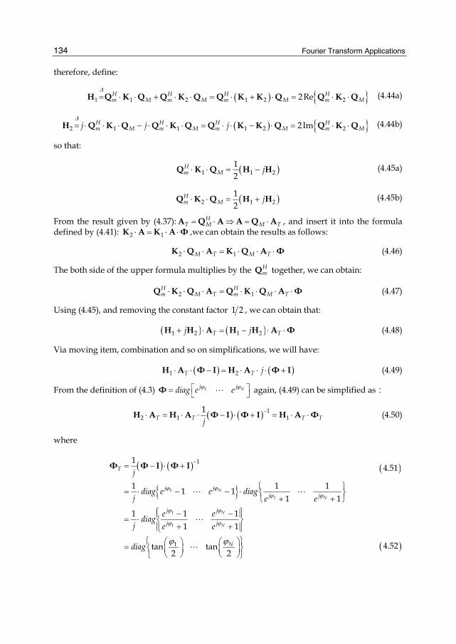
Fourier Transform Applications
134
therefore, define:
( ) { }1 1 2 1 2 22ReH H H Hm M m M m M m M
Δ= ⋅ ⋅ + ⋅ ⋅ = ⋅ + ⋅ = ⋅ ⋅H Q K Q Q K Q Q K K Q Q K Q (4.44a)
( ) { }2 1 1 1 2 22 ImH H H Hm M m M m M m Mj j j
Δ= ⋅ ⋅ ⋅ − ⋅ ⋅ ⋅ = ⋅ ⋅ − ⋅ = ⋅ ⋅H Q K Q Q K Q Q K K Q Q K Q (4.44b)
so that:
( )1 1 212
Hm M j⋅ ⋅ = −Q K Q H H (4.45a)
( )2 1 212
Hm M j⋅ ⋅ = +Q K Q H H (4.45b)
From the result given by (4.37): HT M M T= ⋅ ⇒ = ⋅A Q A A Q A , and insert it into the formula
defined by (4.41): 2 1⋅ = ⋅ ⋅K A K A Φ ,we can obtain the results as follows:
2 1M T M T⋅ ⋅ = ⋅ ⋅ ⋅K Q A K Q A Φ (4.46)
The both side of the upper formula multiplies by the HmQ together, we can obtain:
2 1H Hm M T m M T⋅ ⋅ ⋅ = ⋅ ⋅ ⋅ ⋅Q K Q A Q K Q A Φ (4.47)
Using (4.45), and removing the constant factor 1 2 , we can obtain that:
( ) ( )1 2 1 2T Tj j+ ⋅ = − ⋅ ⋅H H A H H A Φ (4.48)
Via moving item, combination and so on simplifications, we will have:
( ) ( )1 2T T j⋅ ⋅ − = ⋅ ⋅ ⋅ +H A Φ I H A Φ I (4.49)
From the definition of (4.3) 1 Nj jdiag e eϕ ϕ⎡ ⎤= ⎣ ⎦Φ again, (4.49) can be simplified as:
( ) ( ) 12 1 1
1T T T Tj
−⋅ = ⋅ ⋅ − ⋅ + = ⋅ ⋅H A H A Φ I Φ I H A Φ (4.50)
where
( ) ( )
{ }1
1
1
1
1
1
1
1 1 11 11 1
1 1 11 1
tan tan2 2
N
N
N
N
T
j jj j
j j
j j
N
j
diag e e diagj e e
e ediagj e e
diag
ϕ ϕϕ ϕ
ϕ ϕ
ϕ ϕ
ϕϕ
−= − ⋅ +
⎧ ⎫= ⋅ − − ⋅ ⎨ ⎬+ +⎩ ⎭
⎧ ⎫− −⎪ ⎪= ⋅ ⎨ ⎬+ +⎪ ⎪⎩ ⎭
⎧ ⎫⎛ ⎞⎛ ⎞= ⎨ ⎬⎜ ⎟ ⎜ ⎟⎝ ⎠ ⎝ ⎠⎩ ⎭
Φ Φ I Φ I
( )
( )
4.51
4.52
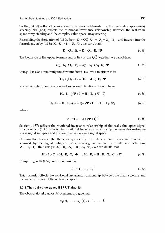
Robust Beamforming and DOA Estimation
135
So that, (4.50) reflects the rotational invariance relationship of the real-value space array steering, but (4.51) reflects the rotational invariance relationship between the real-value space array steering and the complex value space array steering.
Resembling the derivation of (4.50), from HS M S S M S= ⋅ ⇒ = ⋅E Q U U Q E , and insert it into the
formula given by (4.38): 2 1S S⋅ = ⋅ ⋅K U K U Ψ , we can obtain:
2 1M S M S⋅ ⋅ = ⋅ ⋅ ⋅K Q E K Q E Ψ (4.53)
The both side of the upper formula multiplies by the HmQ together, we can obtain:
2 1H HM M S M M S⋅ ⋅ ⋅ = ⋅ ⋅ ⋅ ⋅Q K Q E Q K Q E Ψ (4.54)
Using (4.45), and removing the constant factor 1 2 , we can obtain that:
( ) ( )1 2 1 2S Sj j+ ⋅ = − ⋅ ⋅H H E H H E Ψ (4.55)
Via moving item, combination and so on simplifications, we will have:
( ) ( )2 1S Sj⋅ ⋅ + = ⋅ ⋅ −H E Ψ I H E Ψ I (4.56)
( ) ( ) 12 1 1S S S Tj −⋅ = ⋅ ⋅ − ⋅ + = ⋅ ⋅H E H E Ψ I Ψ I H E Ψ (4.57)
where
( ) ( ) 1T j −= − ⋅ +Ψ Ψ I Ψ I (4.58)
So that, (4.57) reflects the rotational invariance relationship of the real-value space signal subspace, but (4.58) reflects the rotational invariance relationship between the real-value space signal subspace and the complex value space signal space.
Utilizing the character that the space spanned by array direction matrix is equal to which is spanned by the signal subspace, so a nonsingular matrix TT exists, and satisfying
T S T= ⋅A E T , thus using (4.50): 2 1T T T⋅ = ⋅ ⋅H A H A Φ , we can obtain that:
12 1 2 1S T S T T S S T T T
−⋅ ⋅ = ⋅ ⋅ ⋅ ⇒ ⋅ = ⋅ ⋅ ⋅ ⋅H E T H E T Φ H E H E T Φ T (4.59)
Comparing with (4.57), we can obtain that:
1T T T T
−= ⋅ ⋅Ψ T Φ T (4.60)
This formula reflects the rotational invariance relationship between the array steering and the signal subspace of the real-value space.
4.3.3 The real-value space ESPRIT algorithm
The observational data of M elements are given as:
( ) ( )1 , , Mx t x t , 1,t L=

Fourier Transform Applications
136
Step 1. Construct the M L× observational data matrix ( ) ( )1 , , L= ⎡ ⎤⎣ ⎦X x x , where ( ) ( ) ( )1 , , T
Mt x t x t= ⎡ ⎤⎣ ⎦x is the observational data vector which is consists of M elements observational signals.
Step 2. Get the estimating formula of R by ( )1 H
L
∧= ⋅R X X , and transform the received
array data into real-value space T∧R via (4.32).
Step 3. Compute the eigendecompositions of the real-value space T∧R , and get the signal
subspace S∧E , and the source number N
∧.
Step 4. Solve the rotational invariance of (4.57) by least square method (or total least square
method), and gain T∧Ψ .
Step 5. Compute the eigendecompositions of T∧Ψ , where
1
T T T T
−∧ ∧ ∧ ∧= ⋅ ⋅Ψ T Φ T , get
{ }1 , ,TN
diag Ω Ω ∧
∧=Φ .
Step 6. If T∧Φ is the real diagonal matrix, according as (4.3) and (4.52), compute the DOA of
imping signal as fellows:
( )2 arctan
1, ,arcsin
2
k k
k kk N
ϕ Ω
λθ ϕπ Δ
∧⎧ = ⋅⎪ ⎛ ⎞
⎛ ⎞ =⎨ ⎜ ⎟= ⋅⎜ ⎟ ⎝ ⎠⎪ ⎜ ⎟⋅⎝ ⎠⎩
(4.61)
If kΩ 1, ,k N∧⎛ ⎞
=⎜ ⎟⎝ ⎠
is complex, compute the DOA by (4.61) with the real part of kΩ .
4.4 Simulations
In order to validating the correctness and the effective of the proposed algorithm, we present some simulation results to illustrate the performance of RVS-ESPRIT. We consider a ULA with M=8 element and the interelement space is equal to a half of wavelength. There are three signals impinge on the array from 1 80θ = − , 2 20θ = − , 3 40θ = . The detailed simulation results are shown as Fig. 26. ~ Fig. 29.
Fig. 26. and Fig. 27. depicts DOA departure versus snapshot number results of RVS-ESPRIT and TLS-ESPRIT respectively, where the SNR=5dB. In figure 26. and 27., the x-axis denotes the snapshot number, and y-axis denotes the departure of signal DOA.
Fig. 28. and Fig. 29. depicts DOA departure versus SNR results of RVS-ESPRIT and TLS-ESPRIT respectively, where the snapshot number =1000. In figure 28. and 29., the x-axis denotes the SNR, and y-axis denotes the departure of signal DOA.
From the detecting results and comparison between RVS-ESPRIT and TLS-ESPRIT, we can conclude that RVS-ESPRIT can detect DOA of signal quickly and effectively. At the same time, the results validate the correctness and effective of this algorithm.
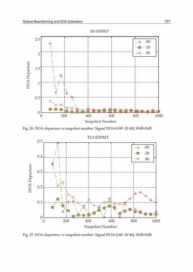
Robust Beamforming and DOA Estimation
137
2.5
2
1.5
1
0.5
0
DO
A D
epar
ture
RS ESPRIT
-80-20 40
0 200 400 600 800 1000Snapshot Number
Fig. 26. DOA departure vs snapshot number. Signal DOA=[-80 -20 40], SNR=5dB
0.5
0.4
0.3
0.2
0.1
0
DO
A D
epar
ture
TLS ESPRIT
-80-20 40
0 200 400 600 800 1000Snapshot Number
Fig. 27. DOA departure vs snapshot number. Signal DOA=[-80 -20 40], SNR=5dB

Fourier Transform Applications
138
25
20
15
10
5
0
DO
A D
epar
ture
RS ESPRIT
-80-20 40
-10 5 0 5 10SNR
Fig. 28. DOA departure versus SNR. Signal DOA=[-80 -20 40], Snapshot number =1000
0.7
0.6
0.5
0.4
0.3
0.2
0.1
0
DO
A D
epar
ture
TLS ESPRIT
-80-20 40
-10 -5 0 5 10SNR
Fig. 29. DOA departure versus SNR. Signal DOA=[-80 -20 40], Snapshot number =1000
Robust Beamforming and DOA Estimation
139
4.5 Conclusion
This chapter carrys on the detailed theories analysis of RVS-ESPRIT based on the theory of CS-ESPRIT, and gives the concrete implementing algorithm. Because the eigendecompositions of RVS-ESPRIT is in real domain, so the calculation speed is raised consumedly, then the speed of DOA estimating is improved largely also. Due to the inherent forward-backward averaging effect, RVS-ESPRIT can separate two completely coherent sources and provides improved estimates for correlated signals.
5. References [1] J. Capon. High resolution frequency-wavenumber spectrum analysis. Proc. IEEE, Vol.57,
pp: 1408-1418, Aug.1969. [2] J. S. Reed, J. D. Mallet, L. E. Brennan. Rapid convergence rate in adaptive arrays. IEEE
Trans. Aerosp. Electron. Syst., Vol. AES-10, No.6, pp: 853-863, Nov.1974. [3] D. H. Johnson, D. E. Dudgeon. Array signal processing: Concepts and Techniques.
Englewood Cliffs, NJ: Prentice-Hall, 1993. [4] H. Krim, M. Viberg. Two decades of array signal processing research. IEEE Signal
Process. Mag., Vol.13, No.4, pp: 67-94, Jul.1996. [5] L. C. Godara. Application of antenna arrays to mobile communications, Part II: Beam-
forming and direction-of-arrival considerations. Proc. IEEE, Vol.85, No.8, pp: 1195-1245, Aug.1997.
[6] H. L. Van Trees. Detection, estimation, and modulation theory, Part IV, Optimum array processing. New York: Wiley, 2002.
[7] P. S. Naidu. Sensor array signal processing. Boca Raton, FL: CRC, 2001. [8] J. R. Guerci. Space-time adaptive processing. Norwood, MA: Artech House, 2003. [9] Jian Li, Petre Stotica. Robust adaptive beamforming. New York: Wiley, 2006. [10] H. Cox. Resolving power and sensitivity to mismatch of optimum array processors.
J. Acoust. Soc. Amer., Vol.54, No.3, pp: 771-785, Mar.1973. [11] D. D. Feldman, L. J. Griffiths. A projection approach to robust adaptive beamforming.
IEEE Trans. Signal Processing, Vol.42, pp: 867-876, Apr.1994. [12] M. Wax, Y. Anu. Performance analysis of the minimum variance beamformer in the
presence of steering vector errors. IEEE Trans. Signal Processing, Vol.44, pp: 938-947, Apr.1996.
[13] E. K. Hung, R. M. Turner. A fast beamforming algorithm for large arrays. IEEE Trans. Aerosp. Electron. Syst., Vol.AES-19, pp: 598-607, Jul.1983.
[14] B. D. Carlson. Covariance matrix estimation errors and diagonal loading in adaptive arrays. IEEE Trans. Aerosp. Electron. Syst., Vol.24, pp: 397-401, Jul.1988.
[15] M. Wax, Y. Anu. Performance analysis of the minimum variance beamformer. IEEE Trans. Signal Processing, Vol.44, pp: 928-937, Apr.1996.
[16] H. Cox, R. M. Zeskind, M. H. Owen. Robust adaptive beamforming. IEEE Trans. Acoust., Speech, Signal Processing, Vol.ASSP-35, pp:1365-1376, Oct.1987.
[17] A. B. Gershman. Robust adaptive beamforming in sensor arrays. Int. J. Electron. Commun., Vol.53, pp: 305-314, Dec.1999.
[18] A. B. Gershman. Robust adaptive beamforming: an overview of recent trends and advances in the field. International Conference on Antenna Theory and Technique, 9-12 September, 2003, Sewstopol, Ukraine, pp: 30-35.

Fourier Transform Applications
140
[19] Sergiy A. Vorobyov, A. B. Gershman, Zhi-Quan Luo. Robust adaptive beamforming using worst-case performance optimization: a solution to the signal mismatch problem. IEEE Trans. Signal Processing. Vol.51, No.2, pp: 313-324, Feb.2003.
[20] Jian Li, Petre Stotica, Zhisong Wang.On robust capon beamformer and diagonal loading. IEEE Trans. Signal Processing. Vol.51, No.7, pp: 1702-1715, Jul.2003.
[21] S. Shahram, A. B. Gershman, Zhiquan Luo, et al. Robust adaptive beamforming for general-rank signal models. IEEE Trans. Signal Processing, Vol.51, No.9, pp: 2257-2269, Sep.2003.
[22] Jian Li, Petre Stotica, Zhisong Wang, Doubly constrained robust capon beamformer. IEEE Trans. Signal Processing. Vol.52, No.9, pp: 2407-2423, Sep.2004.
[23] G.L. Robert, P.B. Stephen. Robust minimum variance beamforming. IEEE Trans. Signal Processing, Vol.53, No.5, pp: 1684-1696, May.2005.
[24] Ayman Elnashar, Said M. Elnoubi, Hamdi A. El-Mikati. Further study on robust adaptive beamforming with optimum diagonal loading. IEEE Trans. Antennas Propagation, Vol.AP-54, No.12, pp: 3647-3658, Dec.2006.
[25] C.Y.Chen, P.P.Vaidyanathan. Quadratically constrained beamforming robust against direction-of- arrival mismatch. IEEE Trans. Signal Processing, Vol.55, No.8, pp: 4139-4150, Aug.2007.
[26] R. A. Monzingo, T. W. Miller. Introduction to adaptive arrays. New York: Wiley, 1980. [27] Z. Tian, K. L. Bell, H. L. Van Trees. A recursive least squares implementation for LCMP
beamforming under quadratic constraint. IEEE Trans. Signal Processing, Vol.49, No.6, pp: 1365-1376, Jun.2001.
[28] L. C. Godara. Error analysis of the optimal antenna array processors. IEEE Trans. Aerosp. Electron. Syst., Vol. AES-22, pp: 395-409, Jul.1986.
[29] K. L. Bell, Y. Ephraim, H. L. Van Trees, A Bayesian approach to robust adaptive beamforming. IEEE Trans. Signal Processing, Vol.48, pp: 386-398, Feb.2000.
[30] L. Chang, C. C. Yeh. Performance of DMI and eigenspace-based beamformers. IEEE Trans. Antennas Propagation, Vol.40, pp: 1336-1347, Nov.1992.
[31] Cheng-Chou Lee, Ju-Hong Lee. Eigenspace-based adaptive array beamforming with robust capabilities. IEEE Trans. Antennas Propagation, Vol.45, pp: 1711-1716, Dec.1997.
[32] J. Riba, J. Goldberg, G. Vazquez. Robust beamforming for interference rejection in mobile communications. IEEE Trans. Signal Processing, Vol.45, pp: 271-275, Jan.1997.
[33] J. R. Guerci. Theory and application of covariance matrix tapers for robust adaptive beamforming. IEEE Trans. Signal Processing, Vol.47, pp: 997-985, Apr.1999.
[34] J. R. Guerci, J.S.Bergin. Principal components,covariance matrix tapers,and the subspace leakage problem. IEEE Trans. Aerosp. Electron. Syst, Vol.38, pp: 152-162, Jan.2002.
[35] F. Vincent, O. Besson. Steering vector errors and diagonal loading, IEE Proceedings.-Radar Sonar Navig., Vol.151, No.6, pp: 337-343, Dec.2004.
[36] O. Besson, F. Vincent. Performance analysis of beamformers using generalized loading of the covariance matrix in the presence of random steering vector errors. IEEE Trans. Signal Processing, Vol.53, pp: 452-459, Feb.2005.
[37] Almir Mutapcic, Seung-Jean Kim, Stephen Boyd. Beamforming with uncertain weights. IEEE Signal Processing Letter, Vol.14, No.5, pp: 348-351, May.2007.

Robust Beamforming and DOA Estimation
141
[38] Liu Congfeng, Liao Guisheng, Robust capon beamformer under norm constraint, Signal Processing, May.2010, Vol.90, Issue.5, pp: 1573-1581.
[39] Dolph C L. A current distribution for broadside arrays which optimizes the relationship between beam width and sidelobe level. Proc IRE, June.1946, Vol.34, pp:335–348.
[40] Zhou P, Ingram M. Pattern synthesis for arbitrary arrays using an adaptive array method. IEEE Transactions on Antennas And Propagation. May.1999, Vol.47, No.5, pp:862-869.
[41] Wang F, Balakrishnan V, Zhou P Y, et al. Optimal array pattern synthesis using semidefinite programming. IEEE Transactions on Signal Processing, May.2003, Vol.51, No.5, pp:1172-1183.
[42] Guo Q, Liao G., Wu Y, et al. Pattern synthesis method for arbitrary arrays based on LCMV criterion. Electronics Letters. May.2003, Vol.39, No.23, pp:1628-1630.
[43] Xie Yao, Jian Li, Zheng Xiayu, et al. Optimal array pattern synthesis via matrix weighting, ICASSP, IEEE International Conference on Acoustics, Speech and Signal Processing – Proceedings, Apr 15-20 2007, Honolulu, HI, United States, IEEE Inc., Piscataway, NJ 08855-1331, United States, Vol.2, pp: 885-888.
[44] Kurup D G., Himdi M, Rydberg A. Synthesis of uniform amplitude unequally spaced antenna arrays using the differential evolution algorithm, IEEE Transactions on Antennas And Propagation. Sep.2003, Vol.51, No.9, pp:2210-2217.
[45] Boeringer D W, Werner D H. Particle swarm optimization versus genetic algorithms for phased array synthesis, IEEE Transactions on Antennas And Propagation. Mar.2004, Vol.52, No.3, pp:771-779.
[46] Liu Xiaojun, Liu Congfeng, Liao Guisheng, Improved pattern synthesis method with linearly constraint minimum variance criterion, 2010 IEEE Internation Conference on Wireless Communications, Networking and Information Security (WCNIS2010), 2010.6,25-27, Vol.2, Beijing China。
[47] Barabell A.J, Improving the resolution performance of eigenstructure-based direction-finding algorithms.Proc,ICASSP 83,1983,pp.336-339.
[48] Kumaresan R. and Tufts D.W., Estimating the angles of arrival of multiple plane wave,IEEE Trans,1983,AES-19,pp.134-138.
[49] Bao B and Hari.K, Performance analysis of root-MUSIC, IEEE Trans, 1989, ASSP-37,pp.1939-1949.
[50] Li F and Vaccaro.R.J,Analytical performance prediction of subspace-based algorithms for DOA estimation: SVD and Signal Processing II Algorithms,Analysis and Applications (Elsevier,New York,1991)
[51] Xu X.L and Buckley K.M, Reduced dimension beamspace broad-band localization, preprocessor design and evaluation.Proc.IEEE Forth Workshop on Spectrum Estimation and Modeling, 1988,pp22-26.
[52] Ta sung Lee, Fast implementation of root-form eigen-based methods for detecting closely spaced sources IEE Proceedings-F Vol.139.No.4,August 1992.
[53] Marius P, Alex B.G and Martin H, Unitary root-MUSIC with a real-valued eigendecomposition: a theoretical and experimental performacce study, IEEE Transactions on SP,Vol.48,No.5,May 2000,pp:1306-1314.
[54] Liu Congfeng, Liao Guisheng, Fast algorithm for root-MUSIC with real-valued eigendecomposition, Radar-2006: 2006 CIE International Conference on Radar 2006.10 ShangHai China.
Fourier Transform Applications
142
[55] Q. S Ren and A. J. Willis, Extending MUSIC to single snapshot and on line direction finding applications, International Radar Conference, IEE, Stevenage, United Kingdom, Oct.1997: 783-787.
[56] Liu Xiaojun, Liu Congfeng, Liao Guisheng, Polynomial coefficient finding for root-MUSIC, Journal of Electronic (China), 2009.8, Vol.26(4).
[57] R. Roy and T. Kailath, “ESPRIT-Estimation of signal parameters via rotational invariance techniques,” in Signal Processing Part 11: Control Theory and Applications (L. Auslander, F. A. Griinbaum, J. W. Helton, T. Kailath, P. Khargonekar, and S. Mitter, Eds.). Berlin, Vienna, New York Springer-Verlag, 1990, pp. 36941 1.
[58] R. H. Roy, ”ESPRIT-estimation of signal parameters via rRotational invariance techniques,” Ph.D. thesis, Stanford Univ., Stanford, CA, Aug. 1987.
[59] M. Haardt and M. E. Ali-Hackl, “Unitary ESPRIT: How to exploit additional information inherent in the rotational invariance structure,” in Proc. IEEE Int. ConJ Acoust., Speech, Signal Processing, Adelaide, Australia, Apr. 1994, pp. 229-232, vol. IV.
[60] S. U. Pillai and B. H. Kwon, “Forwardhackward spatial smoothing techniques for coherent signal identification,” IEEE Trans. Acoust., Speech, Signal Processing, vol. 37, pp. 8-15, Jan. 1989.
[61] B. D. Rao and K. V. S. Hari, “Weighted subspace methods and spatial smoothing: Analysis and comparison,” IEEE Trans. Signal Processing, vol. 41, pp. 788-803, Feb. 1993.
[62] Martin Haardt, Josef A. Nossek Unitary ESPRIT: how to obtain increased estimation accuracy with a reduced computational burden IEEE Trans. Signal Processing, Vol. 43, No. 5, pp.1232-1242. MAY 1995
[63] B. Ottersten, M. Viberg, and T. Kailath, “Performance analysis of the total least squares ESPRIT algorithm,” IEEE Trans. Signal P mcessing, vol. 39, pp. 1122-1135, May 1991.
[64] Wang Yongliang, Chen Hui, Peng Yingning, Wan qun Spatial spectrum estimation techniques and algorithm Tsinghua university press Beijing China 2004.
[65] Liu Congfeng, Liao Guisheng, Real-value space ESPRIT algorithm and Its implement, WiCOM 2006: 2006 International Conference on Wireless Communications, Networking, and Mobile Computing 2006.09 WuHan China.

1. Introduction
The solar corona has a very complex and highly dynamic structure. It consists of a largenumber of constantly evolving, loops and filaments, which interact with each other andare closely associated with the local magnetic field. The non-stationary character of solarplasma-magnetic structures manifests itself in various forms of the coronal magnetic loopsdynamics as rising motions, oscillations, meandering, twisting (Aschwanden et al., 1999;Schrijver et al., 1999), as well as in formation, sudden activation and eruption of filamentsand prominences. Energetic phenomena, related to these types of magnetic activity, rangefrom tiny transient brightenings (micro-flares) and jets to large, active-region-sized flaresand coronal mass ejections (CMEs). They are naturally accompanied by different kindsof electromagnetic (EM) emission, covering a wide frequency band from radio waves togamma-rays. Radiation, produced within a given plasma environment, carries an informationon physical and dynamic conditions in a radiating source. This causes an exceptionalimportance of the EM radiation, as a diagnostic tool, for understanding the nature and physicsof various solar dynamic phenomena. As a relatively new, in that context, direction of studyin the traditional branch of the solar microwave radio astronomy appears the analysis of theslow, long-periodic (e.g., > 1 s) fluctuations of the radiation intensity (Khodachenko et al.,2005; Zaitsev et al., 2003).
Microwave radiation from the magnetic loops in solar active regions (e.g., during solarflares) is usually interpreted as a gyro-synchrotron radiation, produced by fast electrons onharmonics of the gyro-frequency νB in the magnetic field B of the loop. In the case of apower-law distribution of electrons in energy as f (E) ∝ E−δ, the intensity of gyro-synchrotronradiation Iν from an optically thin loop (Dulk, 1985; Dulk & Marsh, 1982) is
Iν ∝ B−0.22+0.9δ(sin θ)−0.43+0.65δ, (1)
where θ is the angle between magnetic field and the direction of electromagnetic wavepropagation. For the observed typical values of the electron energy spectrum index 2 ≤ δ ≤ 7this implies the proportionality of intensity to a moderately high power of the background
Analysis of Long-Periodic Fluctuations of Solar Microwave Radiation, as a Way for Diagnostics
of Coronal Magnetic Loops Dynamics Maxim L. Khodachenko1, Albert G. Kislyakov2 and Eugeny I. Shkelev2
1Space Research Institute, Austrian Academy of Sciences, Graz, 2Lobachevsky State University, Nizhny Novgorod,
1Austria 2Russia
5

2 Will-be-set-by-IN-TECH
magnetic field and essential anisotropy of the radiation: Iν ∝ B1.58÷6.08( sin θ)0.87÷4.12.Equation (1) is obtained within an assumption of an optically thin source, when the radiationintensity is proportional to the emissivity ην (Dulk, 1985). According to the estimations inUrpo et al. (1994), a coronal loop with diameter of about 4 × 108 cm is optically thin in theconsidered frequency range for the gyro-synchrotron absorption if the density of fast electronsis < 2 × 109 cm−3. The typical density of > 10 keV electrons in the microwave burst events isusually 106 ÷ 107 cm−3 and therefore, it stays well within the above indicated limit.
It follows from the equation (1) that variations of the loop magnetic field, associated withdisturbances of the electric current in a radiating source, should modulate the intensity ofthe microwave radiation of the loop (Khodachenko et al., 2005; Zaitsev et al., 2003). Anotherorigin for the modulation of intensity of the observed microwave radiation can be due to thequasi-periodic motion (oscillation) of a coronal magnetic loop, containing the radiation source.This mechanism is connected with the anisotropy of the gyro-synchrotron emission, as well aswith the variation of the magnetic field value during the oscillatory motion of the loop, whichboth, according to the equation (1), can result in a quasi-periodic modulation of the receivedsignal (Khodachenko et al., 2006; 2011). Therefore, the analysis of slow modulations of solarmicrowave radiation may be used for the diagnostics of oscillating electric currents in thecoronal loops, as well as for the investigation of large-scale motion of the loops (including looposcillations) in solar active regions. By this, it is natural to expect that structural complexity ofsolar active regions will manifest itself in peculiarities of the emitted radiation.
The dynamic spectra of the long-periodic oscillations, modulating the intensity of microwaveradiation from solar active regions, have been found to contain quite often several spectraltracks, demonstrating a specific temporal behaviour (Zaitsev et al., 1998; 2001a;b; 2003).Khodachenko et al. (2005) considered these multi-track features as an indication that thedetected microwave radiation is produced within a system of a few closely located, magneticloops, having slightly different parameters and involved in a kind of common globaldynamic process. In several cases such slow modulations of solar microwave radiation(with multi-track spectra) were interpreted as the signatures of oscillating electric currents,running within the circuits of moving relative each other inductively connected coronalmagnetic loops (Khodachenko et al., 2006). The dynamics of these electric currents has beendescribed by means of the equivalent electric circuit (LCR-circuit) models of the coronal loops(Khodachenko et al., 2003; Zaitsev et al., 1998) characterized by time-dependent inductanceL, capacitance C, resistance R, as well as mutual inductance coefficients Mj (Khodachenko etal., 2003; 2009). The L, C, R and Mj parameters of electric circuit of a current-carrying loopdepend on shape, scale, position of the loop with respect to other loops, as well as on theplasma parameters and value of the total longitudinal current in the magnetic tube. In thatrespect it is worth to mention that the LCR-circuit model ignores the fact that changes of themagnetic field and related electric current propagate in plasma at the Alfvén speed. It ignoresany short-time variations of plasma parameters, which appear to be averaged in course ofderivation of the LCR model equation (Khodachenko et al., 2009; Zaitsev et al., 2001a). TheLCR approach assumes instant changes of the electric current over the whole electric circuitaccording to the varying potential and ignores all the "propagation effects" related to thesystem MHD modes. The LCR equations correctly describe temporal evolution of electriccurrents in a system of solar magnetic current-carrying loops only at a time scale longerthan the Alfvén wave propagation time. More generally, the equivalent electric circuit modelof a coronal loop tends to emphasize the global electric circuit, obscuring the effects of the
144 Fourier Transform Applications

Analysis of Long-Periodic Fluctuations of Solar Microwave Radiation, as a Way for Diagnostics of Coronal Magnetic Loops Dynamics 3
ambient plasma and details of the magnetic structure. The LCR model approach was appliedin particular for interpretation of the solar microwave burst long-periodic modulations withdrifting modulation frequencies ν(t) in the interval 0.03 ÷ 1 Hz. Based on the analysis of thefrequency drift of the modulations Zaitsev et al. (1998; 2001a; 2003) and Khodachenko et al.(2005) estimated also the values of the electric current in flaring loops (108 ÷ 1011 A), whichappeared to be close to the values obtained by other methods (Hardy et al., 1998; Leka et al.,1996; Moreton & Severny, 1968; Spangler, 2007; Tan et al., 2006).
However, not all long-periodic modulations of solar microwave radiation demonstratefrequency drift and occupy a similar frequency range. Khodachenko et al. (2009) pointedout that the frequency of LCR-oscillations of the electric current, which depends on specificparameters of a coronal loop, usually stays within the interval νLCR ≈ (0.03 ÷ 1) Hz.Therefore, the modulations of the solar microwave radiation intensity with 0.03Hz< ν < 1Hzare very likely to be due to the electric currents, oscillating in LCR-circuits of coronal loops.At the same time, modulations caused by the oscillatory motions of loops that contain theradiation sources, because of their direct connection with the large-scale dynamics of loops,should have typical frequencies < 0.01 Hz and exhibit no drift. Thus, it has been proposed in(Khodachenko et al., 2009) that one should distinguish, when speaking about different kindsof long-periodic modulations of the solar microwave radiation, between the low-frequency (LF)(≈ 0.03÷ 1 Hz) and very-low-frequency (VLF) (< 0.01 Hz) modulations, assuming the first to beconnected with the LCR-oscillations of electric currents in the coronal loops and the second tobe caused by large-scale motions of the radiation sources confined within the oscillating loops.LF modulations (e.g., 0.03÷ 1 Hz) have been studied in details and interpreted in terms of theequivalent electric circuit models of coronal loops in Khodachenko et al. (2005; 2006); Zaitsevet al. (1998; 2001a;b; 2003). They are not considered in this chapter, whereas we addresses herethe VLF modulations (< 0.01 Hz) of solar microwave radiation and their possible relation tothe large-scale dynamics of coronal loops in solar active regions. Some preliminary results onthat subject were reported recently in a short publication Khodachenko et al. (2011), and thepresent paper addresses this topic in more details.
Transverse oscillations of the coronal magnetic loops considered here are triggered by flaresand filament eruptions, i.e. by phenomena in which the significant Lorentz forces are likelyacting in association with the magnetic field adjustments. By this, all considered oscillatingloops have at least one footpoint in the immediate vicinity of a separatrix surface or of aflare ribbon. Using the potential-field extrapolations Schrijver & Brown (2000) demonstratedthat the field lines close to a separatrix surface exhibit strongly amplified displacements inresponse to small displacements in the photospheric "roots". This means that the magneticfield lines in the proximity of separatrix are much more sensitive to changes in the field sourcesthan are the field lines that lie well within domains of connectivity. Speaking about a natureof the observed transversal oscillations of coronal loops Schrijver et al. (2002) address twomodels: (a) transverse waves in coronal loops that act as wave guides and (b) mentionedabove, strong sensitivity of the shape of magnetic field lines near separatrix to changes in thebottom field sources. By this, the authors outline several observational features that favor themodel (b). Based on the extensive study of properties of transverse loop oscillations triggeredby flares, Aschwanden et al. (2002) also concluded that most of the loops do not fit the simplemodel of a kink eigen-mode oscillation. Therefore, the present paper is not dedicated tothe study of MHD oscillations in solar coronal loops. Our goal consists in demonstrationof the fact that quasi-periodic transverse motions of a coronal magnetic loop, which contains
145Analysis of Long-Periodic Fluctuations of SolarMicrowave Radiation, as a Way for Diagnostics of Coronal Magnetic Loops Dynamics

4 Will-be-set-by-IN-TECH
a source of microwave emission, may be connected with a specific modulation of radiationintensity received by a remote observer.
Speaking about other possible mechanisms (besides of the microwave radiation sourcelarge-scale oscillatory motion), which may cause a quasi-periodic modulation of thenon-thermal electron gyro-synchrotron radiation, it is necessary to mention that aquasi-periodically varying flow of the non-thermal electrons may also result in oscillationsof intensity of microwave radiation. Generation of energetic electrons usually is believed tobe associated with the processes of magnetic reconnection during solar flares (Miller et al.,1997). There are also theories which suggest acceleration of particles by the inductive andcharge separation electric fields, build in course of the continuous motion of solar large-scalecoronal magnetic structures (Khodachenko et al., 2003; Zaitsev & Stepanov, 1992). Besidesof that, particle acceleration in a collapsing magnetic trap (Karlický & Kosugi, 2004), in theMHD turbulence (LaRosa & Moore, 1993; Miller et al., 1996), and in shocks (Cargill et al.,1988; Holman & Pesses, 1983) are addressed as secondary possible mechanisms for energeticparticle production. An extended review of particle acceleration processes in solar flares wasrecently published by Aschwanden (2002). In most of these cases the typical periods areshorter than those of the VLF transverse oscillations of coronal loops. On the other hand,there are also models in which VLF large-scale oscillations of coronal loops control the processof generation of energetic particles after the impulsive phase of a flare (Nakariakov et al.,2006). This case, however, deserves a special study, which appears beyond the scope of thepresent paper. Our analysis here is based on the traditional scenario, according to which thenon-thermal particles, produced during a flare in particle acceleration regions (e.g., sites ofmagnetic reconnection or the area of separatrix currents), are injected into oscillating loops.
2. Peculiarities of VLF modulations of microwave radiation related to large-scaletransverse motions of the radiating sources in the oscillating coronal loops
Even taking into account the typical ranges of the modulation frequencies of microwaveradiation (mentioned above), it is usually difficult to identify the modulation mechanismacting in each particular case. Indeed, having in mind only Equation (1) one cannot say forsure if the observed modulation is due to a) the electric current oscillations in the radiationsource or b) the large-scale oscillatory motion of the loop. However, regarding the lastmodulation mechanism, an attention should be paid to the fact that large-scale transverseoscillatory motion of a coronal loop is accompanied by the periodic stress of magnetic fieldcreated in the loop, especially near its footpoints, during each inclination, i.e. two timesper oscillation cycle. This means that the magnetic field strength fluctuates during theoscillatory motion of the loop with a half-period Posc/2 of the loop oscillation. Therefore,according to Equation (1), for a transverse oscillating loop, a properly located observer, inaddition to the modulation caused by the emission diagram motion at the main oscillationfrequency ν0 = 1/Posc, may see in some cases the modulation at the double frequency of theloop oscillation 2ν0, as well as weak higher order harmonics caused by the non-linearity ofEquation (1). However, as it will be shown below the relative amplitude of the higher-orderharmonics, i.e., with numbers > 2 is rather low, and in the most cases only the first twoharmonic frequencies can be detected. The domination of the main and double-frequencyharmonics in the spectrum is caused by implicit presence of these frequencies in the signal,according to the above described character of the radiation modulating factors. Therefore,the presence of the "modulation pairs" in the low-frequency spectra, i.e., the lines which can
146 Fourier Transform Applications

Analysis of Long-Periodic Fluctuations of Solar Microwave Radiation, as a Way for Diagnostics of Coronal Magnetic Loops Dynamics 5
be associated with the main and double frequency of the loop oscillation (ν0 and 2ν0) mayindicate about a transverse oscillatory dynamics of the loop.
Formation of the "modulation pairs" and their higher-order harmonic companions inmulti-line dynamic spectrum of the VLF modulation of microwave radiation emitted froma transverse oscillating coronal loop may be illustrated with a simple model. Let’s supposethat the loop undergoes oscillations in the direction transverse to the loop plane as shown inFigure 1. The loop inclination relative to the vertical direction varies as α(t) = α0 sin(2πν0t),where α0 and ν0 are the angular amplitude and frequency of the loop oscillations, respectively.Assuming that this loop, when oriented vertically, is seen by a remote observer at the angle Θ0,we get that in course of the loop oscillation the viewing angle changes as Θ(t) = Θ0 − α(t).
Irrespectively of the nature of a coronal loop oscillation, the important feature of thelarge-scale transverse motion of the loop, consists in an oscillating magnetic stress, created inthe loop during its quasi-periodic inclinations. Assuming the local transverse disturbance ofthe magnetic field relative its initial vertical direction to be δB, we find that the total disturbedmagnetic field is δB/ cos α(t). For sufficiently small α(t) the following approximation canbe used: 1/(cos α(t)) ≈ 1/(1 − α(t)2)1/2 ≈ 1 + (1/2)α(t)2. This means that the disturbedmagnetic field in the loop varies in time as B(t) ≈ δB(1 + (1/2)α(t)2). Therefore, for theassumed above sinusoidal character of α(t), we finally obtain that the local magnetic field in atransverse oscillating magnetic loop may be approximated as B(t) ∝ (1 + 0.5α2
0 sin2(2πν0t)).Substitution of the expressions for Θ(t) and B(t) into (1) enables to construct a modelingsignal for the varying intensity of microwave radiation emitted from a transverse oscillatingmagnetic loop. The examples of dynamic spectra of this signal obtained with α0 = π/6 andδ = 5 for different viewing angles Θ0 = π/2; π/3; π/4; π/6 are shown in Figure 2.
Dynamical spectra of the modeling signal in Figure 2 demonstrate several important features,typical for the radiation emitted from a microwave source located in a transverse large-scaleoscillating magnetic loop, which may be observed in the solar microwave emission. Inparticular, for the most of the viewing angles (except of Θ0 = π/2) the dynamic spectracontain well pronounced "modulation pairs", e.g. the lines at the main ν0 and double 2ν0frequency of the oscillation. Besides of that, sometimes also a weak third harmonic at 3ν0may be observed, which appears due to essentially non-sinusoidal (non-harmonic) characterof the signal resulted from the joint action of two modulating factors: quasi-periodic magneticstress and emission diagram motion. In a special case of Θ0 = π/2, the absence of the mainfrequency component is caused by a "symmetrizing" (in this case) of the varying angular partof the emission intensity. This results in a situation when the diagram motion and magneticstress factors work synchronously.
As it can be seen in Figure 2, only the first two harmonics have high enough amplitudes. Inparticular, the spectral amplitude of third harmonic in the cases with Θ0 = π/3; π/4; π/6,never exceeds 25% of the main frequency component, whereas the second harmonicconstitutes usually about 65% of the last. Therefore, the detection of harmonics with numbershigher than 2 in a natural signal, will be in the most cases difficult due to the noisecontamination. The presence of modulation pairs in the VLF spectra of solar microwaveradiation may be considered as an imprint of a transverse kink-type motion of a loopcontaining the radiation source. This feature may be used for the indirect identification ofcandidates for transverse oscillating coronal loops by finding specific modulation lines in theVLF dynamic spectra of microwave radiation. However, the exact detection of transverse
147Analysis of Long-Periodic Fluctuations of SolarMicrowave Radiation, as a Way for Diagnostics of Coronal Magnetic Loops Dynamics

6 Will-be-set-by-IN-TECH
Fig. 1. Schematic view of an oscillating loop which contains a microwave radiation source.Θ0 is the direction to a remote observer and α0 is the angular amplitude of the looposcillations.
motion of the radiating loops by the dynamical spectra of microwave emission (with theexclusion of other mechanisms which may also generate higher spectral harmonics) requiresquantitative study of the measured radio signal and superimposing these results with theprecise calculation of the radiation from the loop, taking into account the loop position relativeobserver.
Several real observational examples are considered below, for which VLF modulations ofmicrowave radiation could be associated with the observed in EUV post-flare oscillatingcoronal loops.
148 Fourier Transform Applications
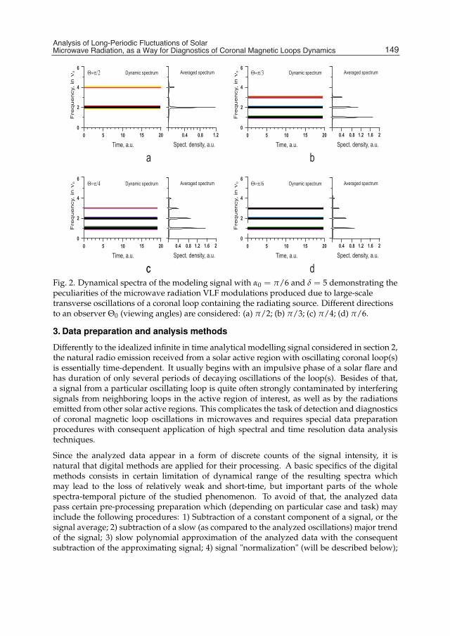
Analysis of Long-Periodic Fluctuations of Solar Microwave Radiation, as a Way for Diagnostics of Coronal Magnetic Loops Dynamics 7
Fig. 2. Dynamical spectra of the modeling signal with α0 = π/6 and δ = 5 demonstrating thepeculiarities of the microwave radiation VLF modulations produced due to large-scaletransverse oscillations of a coronal loop containing the radiating source. Different directionsto an observer Θ0 (viewing angles) are considered: (a) π/2; (b) π/3; (c) π/4; (d) π/6.
3. Data preparation and analysis methods
Differently to the idealized infinite in time analytical modelling signal considered in section 2,the natural radio emission received from a solar active region with oscillating coronal loop(s)is essentially time-dependent. It usually begins with an impulsive phase of a solar flare andhas duration of only several periods of decaying oscillations of the loop(s). Besides of that,a signal from a particular oscillating loop is quite often strongly contaminated by interferingsignals from neighboring loops in the active region of interest, as well as by the radiationsemitted from other solar active regions. This complicates the task of detection and diagnosticsof coronal magnetic loop oscillations in microwaves and requires special data preparationprocedures with consequent application of high spectral and time resolution data analysistechniques.
Since the analyzed data appear in a form of discrete counts of the signal intensity, it isnatural that digital methods are applied for their processing. A basic specifics of the digitalmethods consists in certain limitation of dynamical range of the resulting spectra whichmay lead to the loss of relatively weak and short-time, but important parts of the wholespectra-temporal picture of the studied phenomenon. To avoid of that, the analyzed datapass certain pre-processing preparation which (depending on particular case and task) mayinclude the following procedures: 1) Subtraction of a constant component of a signal, or thesignal average; 2) subtraction of a slow (as compared to the analyzed oscillations) major trendof the signal; 3) slow polynomial approximation of the analyzed data with the consequentsubtraction of the approximating signal; 4) signal "normalization" (will be described below);
149Analysis of Long-Periodic Fluctuations of SolarMicrowave Radiation, as a Way for Diagnostics of Coronal Magnetic Loops Dynamics

8 Will-be-set-by-IN-TECH
and 5) digital filtration of contaminating components. Altogether, the "subtraction" methods1-3 enhance visibility of weaker fluctuations of the radiation, enabling better analysis of theirspectral and temporal characteristics. Note, that the digital filtration (e.g., the method 5) withan appropriate filter(s) may efficiently substitute all the "subtraction" methods. However, theinertness of a filter results in some smoothing of the radio emission fluctuations of interest.Besides of that, information about the intensity of the radiation fluctuations is lost during thefrequency filtration.
The filtration algorithm consists in the application of a Gaussian window to the analyzedsignal spectrum, obtained with the discrete Fourier transform (DFT), with the consequentperformance of the reverse DFT. The Gaussian window for the low frequency (LF), highfrequency (HF), band-pass (BP), and band-lock (BL) filters, respectively, is determined by thefollowing expressions:
WLF(k) = exp{− k2
2 ·(
f1fs· d · N
)−2}
, k = 0, ..., N/2;
WHF(k) = 1 − exp{− k2
2 ·(
f1fs· d · N
)−2}
, k = 0, ..., N/2;
WBP(k) = exp{− 1
2 ·(
kN − f0
fs
)2 ·(
Δ ffs
· d)−2
}, k = 0, ..., N/2;
WBL(k) = 1 − exp{− 1
2 ·(
kN − f0
fs
)2 ·(
Δ ffs
· d)−2
}, k = 0, ..., N/2.
(2)
Here N is the number of counts in the analyzed signal, fs is the frequency of discretization, dis decimation coefficient (Marple, 1986), f1 is the cut-off frequency for the LF and HF filters,f0 and Δ f , are the central frequency and the band, respectively, for the BP and BL filters.
Let’s consider now the "normalization" method. It is based on a treatment of an analyticalsignal z(n) (Marple, 1986):
z(n) = s(n) + isH(n) = M(n) exp(iΨ(n)), (3)
where s(n) and sH(n) are the analyzed digital signal and its Hilbert conjugate, respectively,and n is the count number. The parameters M(n) and Ψ(n) are the module and phase of theanalytical signal, which are defined as the following:
M(n) =√
s(n)2 + sH(n)2,Ψ(n) = arctan
[sH(n)s(n)
].
(4)
The "normalization" procedure consists in division of the analytical signal z(n) on M(n). Bythis, the amplitudes of all spectral components of the analyzed process s(n) become to beequalized. Note, that due to the orthogonality of functions s(n) and sH(n), the value offunction M(n) never becomes zero. The "normalization" method is especially efficient forthe analysis of non-stationary modulation processes. It enables to detect and to follow thevariations of an "instantaneous" frequency of an oscillatory component of radiation.
An important role in the present work belongs also to the method, used for the detectionof quasi-periodic features in the time records of the solar microwave radiation intensity. Itconsists in application of an original data analysis algorithm (Shkelev et al., 2002; Zaitsev etal., 2001b) made as a combination of the "sliding window" Fourier (SWF) transform technique
150 Fourier Transform Applications
Analysis of Long-Periodic Fluctuations of Solar Microwave Radiation, as a Way for Diagnostics of Coronal Magnetic Loops Dynamics 9
and the nonlinear Wigner-Ville (WV) method (Cohen, 1989; Ville, 1948; Wigner, 1932). Belowwe outline the idea of this data analysis algorithm and its main features.
The classical Fourier transform enables the analysis of a given signal in terms of separatespectral frequency components. It is applied for the study of relative distribution of energybetween the spectral components in the case of sufficiently long (ideally infinite) durationof the analyzed signal. However such energetic spectrum does not provide an informationon a time when each particular spectral component appears. Possible improvement of theclassical Fourier transform method in that respect consists in its application within a certaininterval of time Δt (so called "window") and in a consequent shift of this "window" alongthe time axis. This approach became a standard method for the analysis of non-stationarysignals. Further generalization of SWF transform method leads to the wavelet analysis, whereeffect of the "window" is produced by means of a certain mother-wavelet function. Wavelettransform enables judging about energy distribution over the time and frequency of ananalyzed signal. Nowadays this method is also widely used for the analysis of non-stationaryand impulsive signals. Its efficiency is however strongly dependent on parameters of theapplied mother-wavelet function, which needs to be specially selected and adjusted to thetype of particular analyzed signal.
Recently one more spectral analysis method has been applied in astrophysics. This method isbased on the Wigner-Ville (WV) transform
P( f , t) =∫ ∞
−∞z(
t +τ
2
)z∗
(t − τ
2
)e−i2π f τdτ, (5)
where z(t) = s(t) + isH(t) is an analytic signal, made of the analyzed sample of real signals(t), and its Hilbert conjugate sH(t). Function P( f , t) gives distribution of the signal energyover frequency f and time, and may be visualized in the form of a dynamical spectrum of thesignal. According to its definition (5), WV transform may be also interpreted as Fourier image(relative the shifted time) of the local autocorrelation function for the analytical signal z(t).
Since the time t appears explicitly among the arguments of the WV spectrum P( f , t), thismethod is most efficient for high-resolution spectra-temporal analysis of non-stationarysignals with varying spectra, such as quasi-harmonic signals with a changing frequency,or varying impulsive signals. In these cases SWF transform and wavelet methods are lessefficient, because the averaging over the analysis window (or over the wavelet) results ina decrease of spectral density of the signal components, varying within the correspondingtime intervals. At the same time, the non-linearity and non-locality of WV method causeappearance of artificial inter-modulation spectral components at combination frequencies(artifacts) and may result also in suppression of weak spectral components of the signal by itsmore intense or noisy parts (Cohen, 1989; Shkelev et al., 2002). To compensate the drawbacksof SWF and WV data analysis methods, when they are used separately, and to keep theirstrong features, the methods were combined in a proper way in the SWF-WV algorithm,which uses various types of signal processing and filtration (with variable shape and sizeof the analysis windows) in order to eliminate possible artifacts and to provide high spectraland temporal resolution (Kislyakov et al., 2011; Shkelev et al., 2002).
To avoid the appearance of spurious spectra caused by the signal edge effects in the caseof analysis of real finite in time signal samples, the so called "weighting" functions withsmoothed edges are used. In the present study, the SWF spectrum Sk of a discrete signal
151Analysis of Long-Periodic Fluctuations of SolarMicrowave Radiation, as a Way for Diagnostics of Coronal Magnetic Loops Dynamics
10 Will-be-set-by-IN-TECH
sn consisting of N counts is calculated by a discrete Fourier transform (DFT) (Allen & Mills,2004; Marple, 1986):
Sk = ∑N−1n=0 wnd(n)sn exp
{−i 2πnk
N
}, k = 0, 1, ..., N − 1 (6)
with a sliding window wnd(n). The following window functions are used (see also Pollock(1999)):
wnd1(n) ={
1 , 0 ≤ n < N0 , n ≥ N – a rectangular window
wnd2(n) ={
cos2 (π·n2N
), 0 ≤ n < N/2
0 , n ≥ N/2– Henning’s window
wnd3(n) =
⎧⎪⎪⎨⎪⎪⎩
1 − 6 ·(
2·nN
)2+ 6 ·
(2·nN
)3, 0 ≤ n < N/4
2 ·(
1 − 2·nN
)3, N/4 ≤ n < N/2
0 , n ≥ N/2
– Parsen’s window.
(7)The advantage of this method consists in its high performance speed, especially if the standardalgorithms of fast Fourier transform (FFT) are used in the calculations (Allen & Mills, 2004;Marple, 1986). On the other hand, frequency resolution of SWF is reverse proportional tothe number of signal counts in the applied window. Therefore the size of window should besufficiently large. This in its turn decreases the temporal resolution of the method. In practice,the choice of particular type and width of the window is determined by dynamical features ofthe analyzed signal.
An algorithm of the discrete WV transform is determined by the following expression:
Pmk = P(mΔt, kΔ f ) = 2Δt2N−1
∑n=0
[zm+nz∗m−n exp
{−i
πnkN
}], {m, k} = 0, 1, 2, ..., 2N, (8)
where zn and z∗n are discrete values of the analyzed complex analytical signal made, asdetermined above, of the real discrete signal and its Hilbert conjugate; Δt is a period ofdiscretization, and Δ f = 1/(4NΔt) is the frequency step. Note, that WV transform resultsin real values only in the case of continuous functions integrated in infinite limits (like in (5)).The discrete WV transform (8) yields a complex function Pmk, which is called as "pseudo-WVtransform" (Cohen, 1989). In that respect in practice only a module of Pmk or its real part areconsidered.
In course of the comparative study performed in Kislyakov et al. (2011); Shkelev et al. (2002)it has been shown that WV data analysis technique enables higher spectral and temporalresolution than that of the SWF. In Shkelev et al. (2002) the efficiency of WV and SWFmethods was checked with various test signals, made as combinations of impulsive andquasi-harmonic processes. By this, along with the meaningful spectrum, WV transformgenerated specific artificial spectral features (due to the non-linearity of the method). It hasbeen shown in that respect that superimposing of the higher resolution WV spectra with thoseof lower resolution provided by SWF, may help to identify and to exclude these artificialspectral features form the consideration. Altogether, combined with each other the described
152 Fourier Transform Applications

Analysis of Long-Periodic Fluctuations of Solar Microwave Radiation, as a Way for Diagnostics of Coronal Magnetic Loops Dynamics 11
above SWF and WV methods provide an efficient data analysis algorithm characterizedby high sensitivity, high spectral and temporal resolution, and ability to detect complexmulti-signal modulations in the analyzed data records, enabling the dynamical spectra ofthese modulations. For successful operation of the SWF-WV algorithm, the sampling cadenceof analyzed data series should provide sufficient number of the data points, e.g. ≥ 10, 000points per realization. The length of the analyzed data series should be consistent withthe time scales of considered dynamic phenomena, i.e. the duration of an analyzed dataset should include at least several periods of the modulating oscillatory component. TheSWF-WV method appears the most efficient for the study of signals with non-stationarycomplex modulations. In such cases the traditional Fourier transform and wavelet methodsare less efficient. This feature of the algorithm has been, in particular, used to distinguishbetween the modulations, possibly caused by the large-scale transverse quasi-periodic motionof the loops, which are the subject of the present study, and the modulations with frequencydrifts related with the electric current LCR-oscillations in the loops.
For the visualization of the whole variety of the detected modulations, so called averagedspectral density plots are produced along with the dynamic spectra by the SWF-WValgorithm. These plots are obtained by averaging of multiple instantaneous cuts of thedynamic spectrum taken at given moments of time, so that short-living modulation featuresalso become clearly seen among the longer lasting modulation lines. These both types ofspectra (dynamic and averaged) enable the detection of the large-scale transverse oscillatorydynamics of the radiating coronal magnetic loops.
The universality of SWF-WV algorithm resulted in its successful application in differentbranches of space physics. The algorithm was used for the diagnostics of intrinsic physical anddynamical conditions in the stellar and planetary systems, solar/stellar winds, as well as insolar and planetary radiation sources and planetary environments (Khodachenko et al., 2006;Kislyakov et al., 2006; Panchenko et al., 2009; Zaitsev et al., 2003; 2004). Nowadays, the linkto SWF-WV data analysis algorithm is available for the scientific community via the on-linecatalogue of models and data analysis tools (http://europlanet-jra3.oeaw.ac.at/catalogue/),developed within the JRA3-EMDAF (European modelling and data analysis facilities) activity(http://europlanet-jra3.oeaw.ac.at/) of the European FP7 research infrastructure projectEuroplanet-RI.
4. Diagnostics of large-scale oscillations of coronal loops by the analysis of VLFmodulations of microwave radiation
5. Instrumentation and modulations detection capabilities
We analyze the VLF (< 0.01 Hz) modulations of solar microwave bursts recorded inMetsähovi Radio Observatory (Finland) with the 14-m and 1.8 m radio telescope antenna at 37GHz and 11.7 GHz, respectively. The key selection criterion for the analyzed microwave datawas their synchronism with the oscillating loops observed in extreme ultraviolet (EUV) byTRACE (Aschwanden et al., 2002). The width of the antenna beam pattern of the Metsähoviradio telescope at 37 GHz is 2.4’, the sensitivity of the receiver is about 0.1 sfu (10−23
W m−2 Hz−1), and time resolution, 0.05 ÷ 0.1 s. Therefore, at 37 GHz the spatial resolution ofthe radio telescope is sufficient for identification of an active region that contains a radiatingsource. This enables to analyze microwave radiation emitted directly from the region, imagedin EUV (e.g., observed by TRACE), and to perform the comparison of the radiation features
153Analysis of Long-Periodic Fluctuations of SolarMicrowave Radiation, as a Way for Diagnostics of Coronal Magnetic Loops Dynamics

12 Will-be-set-by-IN-TECH
and dynamics of coronal loops. At 11.7 GHz the radiation is collected from the whole solardisk and the position of the radiating source cannot be resolved. However, even in thiscase, by comparison with observations in other wavelengths and timing of the events, it isusually possible to identify the microwave radiation features related to the energy release anddynamic phenomena in particular active regions.
Variations of the background magnetic field in a radiating source may cause not only theamplitude modulation of microwave radio emission from solar active regions (according (1)),but also could result in a certain frequency modulation (due to the dependence of electrongyro-frequency νB on the magnetic field). The estimated width of the gyro-frequency variationinterval due to this effect is from several tens to several hundreds MHz. At the same time,the bandwidth of the receiver at Metsähovi is much larger than this interval and a possiblefrequency modulation of the microwave radio emission cannot be resolved. Thus, one candetect only the effects of varying magnetic field, manifested in the intensity modulation of themicrowave signal, due to (1).
5.1 Observations and interpretation
In this subsection, we show how the analysis of long-periodic modulations of solar microwaveradiation accompanying the explosive events on the Sun may be used to obtain information onthe details of large-scale dynamics of the coronal loops associated with flares and the overallstructure of solar active regions. By this, the primary focus here is made on VLF modulationsof the radiation, emitted from active regions where TRACE observed in EUV at the sametime the large-scale oscillations of coronal loops. Careful check of the solar microwave radioemission records available at Metsähovi revealed several events which coincide in time withthe EUV observations of oscillating coronal loops. Below these events are considered indetails.
Figure 3c shows the intensity profile and dynamic spectrum of VLF modulations ofmicrowave emission from the active region AR8910 on the limb (see Figure 3a,b) where agroup of oscillating loops (Figure 4a) was observed by TRACE after M2.0 flare on 2000-Mar-23,at 11:30-12:00 UT (Aschwanden et al., 2002). These observations were performed at 37 GHz,and the spatial resolution of the Metsähovi radio telescope was sufficient to resolve theradiating source in the active region AR8910.
A remarkable feature of the VLF modulation dynamic spectrum in Fig. 3c,d and the averagedspectral density plot in Fig. 3d consists in the presence of several "modulation pairs". Theseare the modulations (a) at 1.7 mHz (∼ 10 min) and 3.4 mHz (∼ 4.9 min); (b) at 6.0 mHz (∼ 2.8min) and 12.0 mHz (∼ 1.4 min), as well as (c) at 7.8 mHz (∼ 2.1 min) and 15.6 mHz (∼ 64s). According to the considerations in Section 2, these "modulation pairs" could indicate thetransverse oscillating loops with the periods, corresponding to the main frequencies of thepairs, i.e. ∼ 10 min; ∼ 2.8 min, and ∼ 2.1 min for the cases (a), (b), and (c), respectively. Bythis, the first "modulation pair" (case (a)) as a signature of the loop transverse oscillation witha period ∼ 10, fits quite well the results of TRACE observations, which found the oscillatingloop with approximately the same period (615 s) (Aschwanden et al., 2002; Schrijver et al.,2002). As it can be seen from the dynamical spectrum in Figure 3c, the spectral resolution ofthe analysis performed in this particular case was about 0.3 mHz. By this, the frequency 1.62mHz corresponding to the detected TRACE period of 615 s is definitely within the frequency
154 Fourier Transform Applications

Analysis of Long-Periodic Fluctuations of Solar Microwave Radiation, as a Way for Diagnostics of Coronal Magnetic Loops Dynamics 13
c
Fre
qu
en
cy,
Hz
Inte
nsi
ty,
a.u
0.01
0.008
0.006
0.004
0.002
0
1E+4
8E+3
4E+3
11:20 11:40 12:00
Time (UT)
d
Re
lativ
esp
ect
ral d
en
sity
Burst on 23.03.2000Spectrum averaged on T=90-240
at 37 Ghz30
25
20
15
10
5
0
0 4 6 8 10 12 14 16
Frequency, mHz2
1.7 mHz
3.4 mHz
6.0 mHz
7.8 mHz8.4 mHz
12.0 mHz
15.6 mHz
Solar burst on 23.03.2000at 37 GHz
Dynamicspectrumburst on2000-Mar-23
a b
SO
HO
/MD
IM
agneto
gra
m,2000-M
ar-
23
SO
HO
/EIT
304
Å,2000-M
ar-
23
Fig. 3. (a) SOHO/MDI Magnetogram of the Sun on 2000-Mar-23, white arrow points at theactive region AR8910; (b) The Sun image in 304 Å on 2000-Mar-23 from SOHO/EIT, whitearrow points at the active region AR8910; (c) Intensity profile and corresponding VLFmodulation dynamic spectrum of the microwave radiation, recorded from the active regionAR8910 on 2000-Mar-23, at 11:30-12:00; Color codes the dynamic spectral relative intensity(arbitrary units), more dark features correspond to stronger (better pronounced)modulations; (d) averaged spectral density of the VLF modulation.
interval 1.7 ± 0.3 mHz of the modulation feature revealed by the analysis of the microwaveradiation.
155Analysis of Long-Periodic Fluctuations of SolarMicrowave Radiation, as a Way for Diagnostics of Coronal Magnetic Loops Dynamics

14 Will-be-set-by-IN-TECH
Fig. 4. (a) Transverse oscillating coronal loops observed by TRACE in the active regionAR8910 after an M2.0 flare on 2000-Mar-23 at 11:30-12:00 UT (Aschwanden et al., 2002); (b)Phase comparison of the ∼ 10 min modulation component of the microwave emission on2000-Mar-23 and the amplitude of the corresponding 615 s oscillation of the TRACE loop.
A higher level of the second harmonic in the modulation pair 1.7 mHz (∼ 10 min) and3.4 mHz (∼ 4.9 min) is very likely due to the fact that in this particular case two differentmechanisms, modulating the microwave emission of the loop, are by chance manifestedsimultaneously. The first mechanism is that considered in this paper, which is connectedwith a large-scale transverse oscillation of the loop. The second mechanism is due tothe parametric resonance between 5-min velocity oscillations in the solar photosphere andacoustic oscillations of coronal magnetic loop modulating the microwave emission (Zaitsevet al., 2008). The effect consists in simultaneous excitation in the loop, which occasionallyappeared to have a resonant frequency close to 10 min, of oscillations with periods ∼5 min,∼10 min, and ∼3 min, which correspond to the 5-min pumping frequency of the photosphericconvection velocity oscillations, subharmonic, and the first upper frequency of the parametricresonance, respectively (Zaitsev et al., 2008; Zaitsev & Kislyakov, 2006).
It makes no sense to search in TRACE data for the signatures of other oscillating loops(cases (b) and (c)), indicated by the VLF modulations of the microwave radiation duringthe 2000-Mar-23 event, since with the usual 40 s image sampling cadence of TRACE andthe 4-point resolution limit of the instrument (Aschwanden et al., 2002) the fastest detectableby TRACE period is about 3 min. The remaining short-periodic "non-paired" modulationfeature at 8.4 mHz (∼ 1.9 min) may also be a part of a "modulation pair", of which thesecond harmonic counterpart could not be resolved in the VLF spectrum due to the strongcontamination of the analyzed microwave signal. Such weak higher harmonic componentsmay be as well a signature of another oscillatory process, which is unrelated to the large-scaletransverse motion of loops, e.g., a sausage-type MHD wave excited in a loop. Detailedanalysis of this special case remains however beyond the scope of the present study.
An additional confirmation of the fact that ∼ 10 min modulation of the microwave radiationemitted from the active region AR8910 on 2000-Mar-23, is connected with the transverse
156 Fourier Transform Applications

Analysis of Long-Periodic Fluctuations of Solar Microwave Radiation, as a Way for Diagnostics of Coronal Magnetic Loops Dynamics 15
oscillatory motion of a coronal loop, shown in Fig. 4a, and that it is in very likely related to themotion of the emission diagram pattern, comes from the graphs in Fig. 4b. This figure enablesphase comparison for the transverse motion of the loop (observed with TRACE Aschwandenet al. (2002)) and the filtered 1.7 mHz (∼ 10 min) component of the radiation. The lastcharacterizes temporal behaviour of the radio emission received from the oscillating loop.The shifted phase (∼ π) means that the maxima and minima of the radiation part controlledby the loop motion correspond to the specific orientations of the loop and are connected witha certain direction of the emission diagram relative to the observer.
The microwave burst on 2001-Sep-07 represents another example of manifestation of thecoronal loop transverse oscillations in modulation of solar radio emissions. The burst wasproduced during M-flare activity at 15:30 UT in the active region AR9601, close to the solardisc center (see Figure 5a,b), where TRACE observed a group of oscillating loops, immediatelyafter the flare (Aschwanden et al., 2002). The corresponding microwave radiation record wasmade at 11.7 GHz with the Metsähovi radio telescope. At this frequency, the Metsähoviantenna cannot resolve the position of a radiating source, and the emission from the wholesolar disk contributed to the analyzed microwave intensity profile. At the same time, as canbe seen in Fig. 5c, which presents the analyzed microwave radiation record with the burstand its VLF modulation dynamic spectrum, the spectral features related to the processes inthe flaring active region AR9601 can easily be identified by timing of the event. In particular,the dynamic spectrum of VLF modulations of the microwave radiation exhibits several lines,which start simultaneously with the impulsive phase of the flare (at 15:30 UT). These may bethe signatures of different oscillating loops excited by the flare. By this, most of the oscillations(e.g. the dynamic spectrum lines) decay at the time intervals > 20 min. Unfortunately forthis particular event it is impossible to determine exact duration of each of these decayingmodulations because the available microwave radiation record does not cover the end of theevent. As it can be seen in Fig. 5c, some of the dynamic spectrum lines continue beyond theanalyzed record time frame.
Three "modulation pairs" can be identified in the dynamic and averaged spectra in Fig. 5c,d:(a) 1.8 mHz (∼ 9.2 min) and 3.6 mHz (∼ 4.6 min); (b) 2.7 mHz (∼ 6.2 min) and 5.4 mHz(∼ 3.1 min); as well as (c) 4.3 mHz (∼ 3.8 min) and 8.6 mHz (∼ 1.9 min), which may bethe signatures of transverse oscillating loops with periods ∼ 9.2 min, ∼ 6.2 min, and ∼ 3.8min, respectively. We note that the loop periods in the cases (a) and (b) are consistent withthe 6-10 min oscillating loops observed with TRACE (Aschwanden et al., 2002), whereas theshorter period oscillation (case (c)) cannot be resolved by TRACE because of the relativelylong image sampling cadence. The modulation at 5.4 mHz (∼ 3.1 min) may also be a weakthird harmonic produced by the 9.2 min oscillating loop. If this is true, then the line at 2.7 mHz(∼ 6.2 min) will have no a pair-companion, and one should exclude the possibility of the ∼ 6.2min transverse oscillating loop. A "non-paired" weak modulation feature at 6.4 mHz (∼ 2.6min) may be a signature of an oscillating loop with not resolved second harmonic. At thesame time, as for the 2000-Mar-23 event, weak short-period harmonics may be the signaturesof oscillatory processes that are unrelated to the transverse motion of a loop, but caused onlyby a changing magnetic field in the radiating source.
The strong modulation line at 0.6 mHz (∼ 27.7 min) should be considered separately from allother modulations mentioned above. The dynamical spectrum in Fig. 5c, as well as a separatestudy of VLF modulations of the microwave radiation recorded before the faring burst at 15:30UT, reveal the presence of the ∼ 27.7 min component also before the flare. In view of the fact
157Analysis of Long-Periodic Fluctuations of SolarMicrowave Radiation, as a Way for Diagnostics of Coronal Magnetic Loops Dynamics
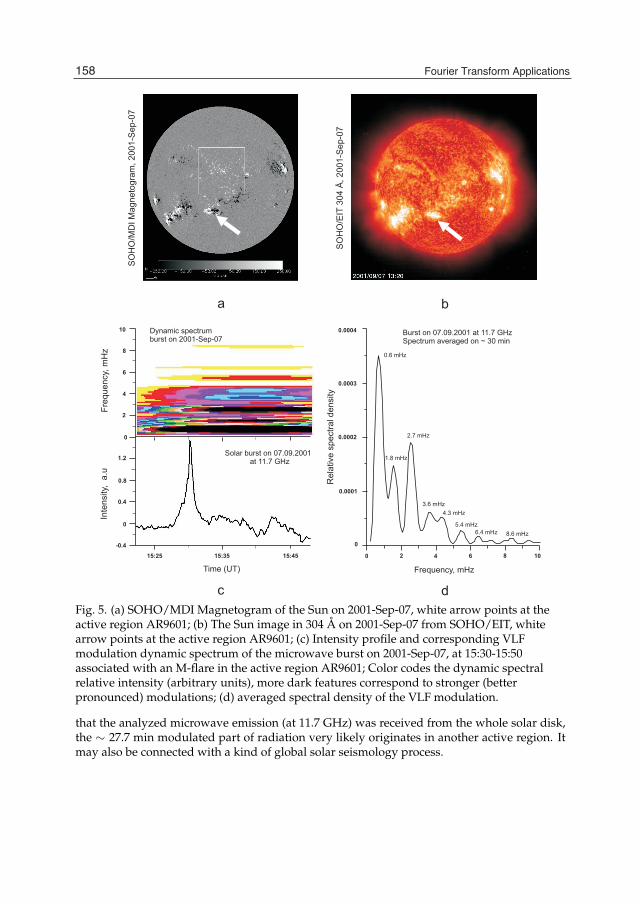
16 Will-be-set-by-IN-TECH
Fig. 5. (a) SOHO/MDI Magnetogram of the Sun on 2001-Sep-07, white arrow points at theactive region AR9601; (b) The Sun image in 304 Å on 2001-Sep-07 from SOHO/EIT, whitearrow points at the active region AR9601; (c) Intensity profile and corresponding VLFmodulation dynamic spectrum of the microwave burst on 2001-Sep-07, at 15:30-15:50associated with an M-flare in the active region AR9601; Color codes the dynamic spectralrelative intensity (arbitrary units), more dark features correspond to stronger (betterpronounced) modulations; (d) averaged spectral density of the VLF modulation.
that the analyzed microwave emission (at 11.7 GHz) was received from the whole solar disk,the ∼ 27.7 min modulated part of radiation very likely originates in another active region. Itmay also be connected with a kind of global solar seismology process.
158 Fourier Transform Applications

Analysis of Long-Periodic Fluctuations of Solar Microwave Radiation, as a Way for Diagnostics of Coronal Magnetic Loops Dynamics 17
The last example of possible manifestation of transverse oscillations of coronal loops inmicrowaves which we present here, is the event on 2001-Sep-15, when TRACE observedoscillating loops, associated with M flare at 11:23 UT in the active region AR9608, close tothe limb (see Figure 6a,b). Similar to the case of the microwave burst on 2001-Sep-07, theevent on 2001-Sep-15 was observed at 11.7 GHz, and the microwave radiation source inAR9608 was not resolved by the Metsähovi antenna. Thus, the emission from the wholesolar disk contributed to the analyzed microwave intensity profile. However, as for theburst on 2001-Sep-07, all the spectral features related to the flaring active region AR9608can be identified by event timing. As it can be seen in Fig. 6c, the dynamic spectrumof VLF modulations of the microwave radiation consists of several lines, most of whichbegin simultaneously with the impulsive phase of the flare at 11:23 UT. These lines may beassociated with oscillatory processes in the active region loops triggered by the flare. All thepost-flare oscillations decay at the time intervals from ∼ 20 min up to ∼ 1 hour.
Fig. 6d shows the averaged spectral density of the VLF modulations of the microwave burston 2001-Sep-15. At least one "modulation pair": 1.3 mHz (∼ 12.8 min) and 2.6 mHz (∼ 6.4min) can be identified among the detected modulation lines. It is very likely connectedwith a transverse oscillating loop having the period ∼ 12.8 min. This result agrees withthe reported TRACE observations of the oscillating loop in the active region AR9608 with aperiod ∼ 12 − 15 min. Other detected in the microwave record on 2001-Sep-15 (see Fig. 6c,d),more short-periodic modulations at 3.8 mHz (∼ 4.4 min) and 5.2 mHz (∼ 3.2 min) couldbe higher-order harmonics produced by the 12.8 min oscillating loop, or the modulationsassociated with oscillatory processes not connected with the transverse motion of loops. Theymay also be the signatures of oscillatory processes in small loops, which cannot be seen inthe TRACE EUV movies due to the limitations of the operated observing mode. Additionallyshould be mentioned a relatively weak line at 0.7 mHz (∼ 23.8 min). Its possible secondharmonic could contribute to the broad line near 1.3 mHz, which is identified as a mainfrequency line in another modulation pair. If that is the case, then this may be a signature ofanother transverse oscillating loop with the period ∼ 23.8 min. Verwichte et al. (2010) reportedrecently detection of such an oscillating loop related with the considered flaring event in thethe active region AR9608.
A special remark deserves also the long lasting ultra-low-frequency (ULF) modulationat 0.3 mHz (∼ 56 min), clearly visible in both, the dynamic and averaged, spectra ofthe long-periodic modulations of solar microwave radiation on 2001-Sep-15 in Figs. 6c,d.Similarly to the 27 min line in the case of the 2001-Sep-07 burst, this ULF modulation appearsbefore the flaring burst and lasts much longer than all other modulation lines in the spectrum(Fig. 6c). Therefore, it cannot be related to the flare in the active region AR9608 and consequentpost-flare dynamics of coronal loops. This modulation feature is probably connected with thesolar seismology processes, or a slow dynamics of another active region. As an additionalargument in support of the solar global i.e., helioseismic nature of the ULF (ν0 < 0.6 mHz,i.e. τ > 30 min) modulations may be the fact that these modulations are usually detectedin the radiation records made at 11.7 GHz when the radio emission from the whole solardisk contributes to the analyzed microwave intensity profile. The radiation emitted fromthe spatially resolved separate active regions, for example, at 37 GHz with Metsähovi radiotelescope, does not exhibit any ULF modulation features. In more details the ULF modulationsof solar microwave radiation are considered in Kislyakova et al. (2011).
159Analysis of Long-Periodic Fluctuations of SolarMicrowave Radiation, as a Way for Diagnostics of Coronal Magnetic Loops Dynamics

18 Will-be-set-by-IN-TECH
c d
Re
lativ
esp
ect
ral d
en
sity
Burst on 15.09.2001Spectrum averaged on ~ 40 min
at 11.7 Ghz,0.0025
0.002
0.0015
0.001
0.0005
0
0 2 3 4 5 6 7
Frequency, mHz
1
3.8 mHz
2.6 mHz
0.3 mHz
1.3 mHz
5.2 mHz
Fre
qu
en
cy,
mH
zIn
ten
sity
,a
.u
10
8
6
4
2
0
Dynamic spectrum,burst on 2001-Sep-15
8
7.5
7
10:00 11:00 12:00
Time (UT)
6.5
6
5.5
14:0013:00
Solar burst on 15.09.2001at 11.7 Ghz
a b
SO
HO
/MD
IM
agneto
gra
m,2001-S
ep-1
5
SO
HO
/EIT
304
Å,2001-S
ep-1
5
0.7 mHz
Fig. 6. (a) SOHO/MDI Magnetogram of the Sun on 2001-Sep-15, white arrow points at theactive region AR9608; (b) The Sun image in 304 Å on 2001-Sep-15 from SOHO/EIT, whitearrow points at the active region AR9608; (c) Intensity profile and corresponding VLFmodulation dynamic spectrum of the microwave burst on 2001-Sep-15, at 11:23-12:15associated with an M-flare in the active region AR9608; Color codes the dynamic spectralrelative intensity (arbitrary units), more dark features correspond to stronger (betterpronounced) modulations; (d) averaged spectral density of the VLF modulation.
5.2 On the magnetic field variations, estimated from VLF spectra
It is impossible, using the available data, to perform an exact calculation for the amplitude ofmagnetic field variations. That is because the analyzed microwave signals were recordedin relative units without calibration to the radiation intensity scale. At the same time,taking into account known values of the maximal intensity measured during the radio
160 Fourier Transform Applications
Analysis of Long-Periodic Fluctuations of Solar Microwave Radiation, as a Way for Diagnostics of Coronal Magnetic Loops Dynamics 19
bursts and the lower limit of sensitivity of the Metsähovi receiver, the intensity modulationamplitude ΔIν can be estimated roughly from the obtained VLF spectra, by their comparisonwith the spectra of specially created modelling signals (Khodachenko et al., 2005). For theconsidered in the paper events this estimation gives the value of the relative variation ofintensity ΔIν/I 0
ν ∼ 10−2 ÷ 10−1. Assuming, as an upper rough limit, that this variation ofintensity is connected only with the varying magnetic field, we come to a relation ΔIν/I 0
ν =(B/B0)
γ − 1 = ((ΔB/B0 + 1)γ − 1), where ΔB/B0 is the relative variation of magnetic field,and γ = −0.22 + 0.9δ is the power index of magnetic field in the equation (1). For 2 < δ < 7one gets that γ = 1.58 ÷ 6.08. For the case of small relative variations of the magnetic field wefinally obtain ΔIν/I 0
ν ≈ γΔB/B0 = 10−2 ÷ 10−1, which for B0 = 100G gives the amplitudeΔB = (0.16 ÷ 6.3) G.
6. Discussion, conclusions and perspectives
The analysis of VLF modulations of solar microwave bursts presented in this work showsgood temporal coincidence of the modulations and their oscillatory parameters with theobserved decaying large-scale transverse oscillations of the coronal loops triggered by flares.This indicates about a physical link between the oscillatory motion of the loops and variationsof the observed radio emission. As a working hypothesis to take this link into account, a loopwith the propagating beams of non-thermal particles which produce microwave emissiondue to the electron gyro-synchrotron mechanism, has been considered. As pointed out bySchrijver et al. (2002), who considered several cases of transverse oscillations of coronal loopsobserved with TRACE (including the event on 2000-Mar-23 addressed in the present paper),in almost all cases the oscillating loops lie at, or near, the large-scale separatrices, or near thesites involved in reconnection. These regions may be the sources of non-thermal particlesinjected into the loops and generating microwave emission there. Moreover, in the case on2000-Mar-23 the loop oscillation happened in response to a flaring event located at the loopbase Schrijver et al. (2002). That could provide a direct input of energetic particles into theloop.
In the most general case, thermal bremsstrahlung mechanism of the radiation should be alsoconsidered, besides of the gyro-synchrotron, for the analyzed frequency range of the solarmicrowave emission. If the last mechanism assumes that there are high energy electronspassing through the magnetic loop, the first one is connected with the radiation of hot plasmaheated by the electron beams in the chromospheric footpoints of the loop. A comparativestudy of contribution of the bremsstrahlung and gyro-synchrotron radiation to the microwaveemission of a flare, performed in Urpo et al. (1994), shows that thermal bremsstrahlungis more important for the microwave events that have an intensity of the order of or lessthan 100 SFU, with the exception of cases when the electron spectrum is sufficiently hard.Therefore, correct interpretation of the microwave radiation source requires considerationof both mechanisms, for example by involving of the hybrid thermal/nonthermal modelof the solar flare emission (Holman & Benka, 1992). However, looking at a possibility ofan oscillatory behaviour of the microwave radiation source which constitutes the primarysubject of the present study, we notice that in the case of the bremsstrahlung mechanismit is possible only for a varying energy deposition into the system, i.e. a varying flow ofnon-thermal particles heating the loop footpoints. In view of the unclearness of how thepost-flare transverse oscillating loop may modulate the source of accelerated electrons, webuilt our analysis with the assumption that the non-thermal particle population remains
161Analysis of Long-Periodic Fluctuations of SolarMicrowave Radiation, as a Way for Diagnostics of Coronal Magnetic Loops Dynamics

20 Will-be-set-by-IN-TECH
more-or-less stable, and all the variations of the observed microwave radiation are connectedwith the non-thermal gyro-synchrotron part of the radiation, modulated by the large-scaleoscillatory motion of the loop. The bremsstrahlung component, even being present in themicrowave radiation, does not contribute to the analyzed oscillating part of the emissionprovided by the gyro-synchrotron mechanism.
Our analysis here is based on the assumption of an optically thin microwave source. In thiscase the radiation intensity is proportional to emissivity ην, given by equation (Dulk, 1985)
ην ≈ 3.3 × 10−2410−0.52δ NB(sin θ)−0.43+0.65δ
(ν
νB
)1.22−0.9δ
, (9)
where ν is radiation frequency, N is the number of electrons per cubic centimeter with energyhigher than 10 keV, B is magnetic field, νB = eB/(2πmec), is the electron-cyclotron frequency,and δ is the electron energy spectrum index. This fact has been used for obtaining our basicequation (1) in Section 1. In the opposite case of an optically thick source, the intensity ofmicrowave radiation is proportional to the effective temperature Te f f , i.e., to the ratio ofemissivity ην and absorption coefficient κν. For the last, Dulk (1985) provides the followingexpression:
κν ≈ 1.4 × 10−910−0.22δ(N/B)(sin θ)−0.09+0.72δ
(ν
νB
)−1.3−0.98δ
. (10)
Therefore, in the case of an optically thick source the dependence of radiation intensity on thevarying magnetic field B(t) and direction to the observer Θ(t) will be different than that givenby the equation (1). However, the character of this dependence, i.e. Iν ∝ (sin(Θ(t)))kB(t)l ,where k and l are the numbers depending on the non-thermal electron spectral index δ, willremain the same. Therefore, one may expect similar manifestation of the varying B(t) andΘ(t) in the modulation of the received microwave emission also in the case of an opticallythick source.
Analysis of LF and VLF modulations of solar microwave radiation is a relatively newdirection in solar radio astronomy which appears nowadays a subject of a certain interest.VLF variations of solar microwave radiation intensity may be related to slow variations ofmagnetic field in a radiating source, as well as to large-scale motions of coronal structurescontaining the radiating source. Joint action of two radiation modulating factors: (i) thequasi-periodic fluctuation of magnetic field and (ii) motion of the radio emission diagram,in the case of a transverse oscillating coronal loop results in essentially non-sinusoidal(non-harmonic) character of the signal received by a remote observer, with stronglypronounced two first harmonics (at the main and double frequency of the oscillation),called here as "modulation pairs". Such specifics of the VLF spectrum has been used forthe identification of transverse oscillating loops triggered by flares. The analysis of solarmicrowave records has been performed with an algorithm based on Sliding Window Fouriertransform and Wigner-Ville techniques. This high sensitive algorithm provides, significantspectral and temporal resolution which enable clear detection of VLF "modulation pairs" inthe solar flaring microwave radiation (microwave bursts). Comparison of parameters of these"modulation pairs" with the simultaneous TRACE observations in EUV of the correspondingsolar active regions enabled to associate some of the paired VLF modulation features with thelarge-scale transverse oscillations of coronal loops. The "non-paired" features also detected
162 Fourier Transform Applications

Analysis of Long-Periodic Fluctuations of Solar Microwave Radiation, as a Way for Diagnostics of Coronal Magnetic Loops Dynamics 21
in the VLF modulation dynamic spectra, may be either parts of "modulation pairs" in whichthe second harmonic cannot be resolved because of the strong contamination of the analyzedsignal, or be the signatures of other oscillatory processes (MHD modes) in the loops, unrelatedto their large-scale transverse motion, e.g., sausage-type MHD waves.
The presence of "modulation pairs" in the VLF spectra of solar microwave radiation isconsidered here as an indication of the transverse oscillating coronal loops. However, theexact characterization of the transverse motion of radiating loops by the dynamical spectraof microwave emission needs a quantitative analysis of the measured radio signal andsuperimposing these results with a precise calculation of the radiation from the loop, takinginto account the loop position relative observer. This topic requires a dedicated study. Itoutlines the general direction for further development of the ideas expressed in the paper.
Besides of that, of certain interest appear the long lasting ULF modulations of solar microwaveradiation detected at < 0.6 mHz (> 30 min) in the absence of bursts, i.e. during the periodsof quiet Sun. It is remarkable that these modulations are not visible in the emissions fromseparate active regions, recorded in particular at 37 GHz with Metsähovi radio telescope. Butthey appear in the integrated radiation received from the whole solar disk at 11.7 GHz. Thisfact may be considered as an argument in support of the global helioseismic nature of theseULF modulations, which also require further more detailed study.
7. Acknowledgements
This work was supported by the Austrian Fond zur Förderung der wissenschaftlichenForschung (project P21197-N16). The authors are thankful to the JRA3/EMDAF(European Modelling and Data Analysis Facility; http://europlanet-jra3.oeaw.ac.at) – asubdivision of the European research infrastructure EUROPLANET-RI and EU FP7 projectIMPEx (http://impex-fp7.oeaw.ac.at) for the support of their research communication andcollaboration visits. The authors would like to thank M.Aschwanden for useful discussionsand the data regarding the transverse large-scale dynamics of coronal loops.
8. References
Allen, R.L. & Mills, D.W. (2004). Signal analysis: time, frequency, scale, and structure. IEEE Press,Wiley-Interscience, ISBN:0-471-23441-9.
Aschwanden, M.J.; Fletcher, L.; Schrijver, C.J.; Alexander, D. (1999). Coronal Loop OscillationsObserved with the Transition Region and Coronal Explorer. The Astrophysical Journal,Vol. 520, No. 2, 880–894, (DOI:10.1086/307502).
Aschwanden, M.J. (2002). Particle acceleration and kinematics in solar flares - A Synthesisof Recent Observations and Theoretical Concepts (Invited Review). Space ScienceReview, Vol. 101, No. 1, 1–227, (DOI:10.1023/A:1019712124366).
Aschwanden, M.J.; DePontieu, B.; Schrijver, C.J.; Title, A. (2002). Transverse Oscillations inCoronal Loops Observed with TRACE II. Measurements of Geometric and PhysicalParameters. Solar Physics, Vol. 206, No. 1, 99–132, (DOI:10.1023/A:1014916701283).
Cargill, P.J.; Goodrich, C.C.; Vlahos, L. (1988). Collisionless shock formation and the promptacceleration of solar flare ions. Astronomy and Astrophysics, Vol. 189, No. 1-2, Jan.,254–262, ISSN 0004-6361.
Cohen, L. (1989). Time-frequency distributions - A review. IEEE Proc., Vol. 77, July-1989,941–981, ISSN 0018-9219.
163Analysis of Long-Periodic Fluctuations of SolarMicrowave Radiation, as a Way for Diagnostics of Coronal Magnetic Loops Dynamics

22 Will-be-set-by-IN-TECH
Dulk, G.A. (1985). Radio emission from the sun and stars. IN: Annual review of astronomy andastrophysics, Vol. 23(A86-14507 04-90), 169–224, Palo Alto, CA, Annual Reviews, Inc.,(DOI:10.1146/annurev.aa.23.090185.001125).
Dulk, G.A. & Marsh, K.A. (1982). Simplified expressions for the gyrosynchrotron radiationfrom mildly relativistic, nonthermal and thermal electrons. The Astrophysical Journal,Vol. 259, Aug-1982, 350–358, (DOI:10.1086/160171).
Hardy, S.J.; Melrose, D.B.; Hudson, H.S. (1998). Observational tests of a double loop model forsolar flares. Publications Astronomical Society of Australia, Vol. 15, No. 3, 318–324.
Holman, G.D. & Benka, S.G. (1992). A hybrid thermal/nonthermal model for the energeticemissions from solar flares. The Astrophysical Journal, Vol. 400, No. 2, L79–L82, ISSN0004-637X, (DOI:10.1086/186654).
Holman, G.D. & Pesses, M.E. (1983). Solar type II radio emission and the shock driftacceleration of electrons. The Astrophysical Journal, Vol. 267, No. 15, 837–843, ISSN0004-637X, (DOI:10.1086/160918).
Karlický, M. & Kosugi, T. (2004). Acceleration and heating processes in acollapsing magnetic trap. Astronomy and Astrophysics, V. 419, 1159–1168,(DOI:10.1051/0004-6361:20034323).
Khodachenko, M.L.; Haerendel, G.; Rucker, H.O. (2003). Inductive electromagnetic effects insolar current-carrying magnetic loops. Astronomy and Astrophysics, Vol. 401, 721–732,(DOI:10.1051/0004-6361:20030146).
Khodachenko, M.L.; Zaitsev, V.V.; Kislaykov, A.G.; Rucker, H.O.; Urpo, S. (2005).Low-frequency modulations in the solar microwave radiation as a possible indicatorof inductive interaction of coronal magnetic loops. Astronomy and Astrophysics, Vol.433, No. 2, 691–699, (DOI:10.1051/0004-6361:20041988).
Khodachenko, M.L.; Rucker, H.O.; Kislaykov, A.G.; Zaitsev, V.V.; Urpo, S. (2006).Microwave Diagnostics of Dynamic Processes and Oscillations in Groups ofSolar Coronal Magnetic Loops. Space Science Reviews, Vol. 122, No. 1-4, 137–148,(DOI:10.1007/s11214-006-7767-0).
Khodachenko, M.L.; Zaitsev, V.V.; Kislyakov, A.G.; Stepanov, A.V. EquivalentElectric Circuit Models of Coronal Magnetic Loops and Related OscillatoryPhenomena on the Sun. (2009). Space Science Reviews, Vol. 149, No. 1-4, 83–117,(DOI:10.1007/s11214-009-9538-1).
Khodachenko, M.L.; Kislyakova, K.; Zaqarashvili, T.V.; Kislyakov, A.G.; Panchenko,M.; Zaitsev, V.V.; Arkhypov, O.V.; Rucker, H.O. (2011). Possiblemanifestation of large-scale transverse oscillations of coronal loops in solarmicrowave emission. Astronomy and Astrophysics, Vol. 525, CiteID A105,(DOI:10.1051/0004-6361/201014860).
Kislyakov, A. G.; Zaitsev, V. V.; Stepanov, A. V.; Urpo, S. (2006). On the Possible Connectionbetween Photospheric 5-Min Oscillation and Solar Flare Microwave Emission. SolarPhysics, Vol. 233, No. 1, 89–106, (DOI:10.1007/s11207-006-2850-y).
Kislyakova, K.G.; Zaitsev, V.V.; Urpo, S.; Riehokainen, A. (2011). Long-period oscillationsof the solar microwave emission. Astronomy Reports, Vol. 55, No. 3, 275–283,(DOI:10.1134/S1063772911030036).
Kislyakov, A.G.; Shkelev, E.I.; Lupov, S.Y.; Kislyakova, K.G. (2011). Parametersof astrophysical objects according to their electromagnetic emission intensitymodulation data. I. Observational data processing algorithms. Bulletin of the NizhnyNovgorod State University, No.2(1), 46–54, (in russian).
164 Fourier Transform Applications

Analysis of Long-Periodic Fluctuations of Solar Microwave Radiation, as a Way for Diagnostics of Coronal Magnetic Loops Dynamics 23
LaRosa, T.N. & Moore, R.L. (1993). A Mechanism for Bulk Energization in the Impulsive Phaseof Solar Flares: MHD Turbulent Cascade. The Astrophysical Journal, Vol. 418, 912–918,(DOI:10.1086/173448).
Leka, K.D.; Canfield, R.C.; McClymont, A.N.; van Driel-Gesztelyi, L. (1996). Evidencefor Current-carrying Emerging Flux. The Astrophysical Journal, Vol. 462, 547–560,(DOI:10.1086/177171).
Marple, S. L., Jr. (1986). Digital spectral analysis with applications. Prentice-Hall, Inc. UpperSaddle River, NJ, USA, ISBN:0-132-14149-3.
Miller, J.A.; LaRosa, T.N.; Moore, R.L. (1996). Stochastic Electron Acceleration by CascadingFast Mode Waves in Impulsive Solar Flares. The Astrophysical Journal, Vol. 461,445–464, (DOI:10.1086/177072).
Miller, J.A.; Cargill, P.J.; Emslie, A.G.; Holman, G.D.; Dennis, B.R.; LaRosa, T.N.; Winglee,R.M.; Benka, S.G.; Tsuneta, S. (1997). Critical issues for understanding particleacceleration in impulsive solar flares. Journal of Geophysical Research, Vol. 102, No.A7, 14631–14660, (DOI:10.1029/97JA00976).
Moreton, G.E. & Severny, A.B. (1968). Magnetic Fields and Flares in the Region CMP 20September 1963. Solar Physics, Vol. 3, No. 2, 282–297, (DOI:10.1007/BF00155163).
Nakariakov, V. M.; Foullon, C.; Verwichte, E.; Young, N. P. (2006). Quasi-periodicmodulation of solar and stellar flaring emission by magnetohydrodynamicoscillations in a nearby loop. Astronomy and Astrophysics, Vol. 452, No. 1, 343–346,(DOI:10.1051/0004-6361:20054608).
Panchenko, M.; Khodachenko, M. L.; Kislyakov, A. G.; Rucker, H. O.; Hanasz, J.; Kaiser, M.L.; Bale, S. D.; Lamy, L.; Cecconi, B.; Zarka, P.; Goetz, K. (2009). Daily variations ofauroral kilometric radiation observed by STEREO, Geophysical Research Letters, Vol.36, No. 6, CiteID L06102, (DOI:10.1029/2008GL037042).
Pollock, D.S.G. (1999). A handbook of time-series analysis, signal processing and dynamics. London:Academic Press, ISBN:0-12-560990-6.
Schrijver, C. J.; Title, A. M.; Berger, T. E.; Fletcher, L.; Hurlburt, N. E.; Nightingale, R. W.; Shine,R. A.; Tarbell, T. D.; Wolfson, J.; Golub, L.; Bookbinder, J. A.; Deluca, E. E.; McMullen,R. A.; Warren, H. P.; Kankelborg, C. C.; Handy, B. N.; de Pontieu, B. (1999). A newview of the solar outer atmosphere by the Transition Region and Coronal Explorer.Solar Physics, Vol. 187, No. 2, 261–302, (DOI:10.1023/A:1005194519642).
Schrijver, C.J.; Aschwanden, M.J.; Title, A.M. (2002). Transverse oscillations in coronal loopsobserved with TRACE I. An Overview of Events, Movies, and a Discussion ofCommon Properties and Required Conditions. Solar Physics, Vol. 206, No. 1, 69–98,(DOI:10.1023/A:1014957715396).
Schrijver, C.J. & Brown, D.S. (2000). Oscillations in the Magnetic Field of the Solar Corona inResponse to Flares near the Photosphere. The Astrophysical Journal, Vol. 537, No. 1,L69–L72, (DOI:10.1086/312753).
Shkelev, E.I.; Kislyakov, A.G.; Lupov, S.Y. (2002). Methods of decreasing of a cross-modulationeffects in the Wigner-Ville distribution. Izv. Vyss. Uchebn. Zaved., Ser. Radiofiz. (transl.as Radiophys. Quantum Electron.), Vol. 45, No. 5, 433-442.
Spangler, S.R. (2007). A Technique for Measuring Electrical Currents in the Solar Corona. TheAstrophysical Journal, Vol. 670, No. 1, 841–848, (DOI:10.1086/521995).
Tan, B.; Ji, H.; Huang, G.; Zhou, T.; Song, Q.; Huang, Y. (2006). Evolution of Electric CurrentsAssociated with Two M-Class Flares. Solar Physics, Vol. 239, No. 1-2, 137–148,(DOI:10.1007/s11207-006-0120-7).
165Analysis of Long-Periodic Fluctuations of SolarMicrowave Radiation, as a Way for Diagnostics of Coronal Magnetic Loops Dynamics

24 Will-be-set-by-IN-TECH
Urpo, S.; Bakhareva, N.M.; Zaitsev, V.V.; Stepanov, A.V. (1994). Comparison of mm-waveand X-ray diagnostics of flare plasma. Solar Physics, Vol. 154, No. 2, 317–334, ISSN0038-0938, (DOI:10.1007/BF00681102).
Verwichte, E.; Foullon, C.; Van Doorsselaere, T. (2010). Spatial Seismology of a Large CoronalLoop Arcade from TRACE and EIT Observations of its Transverse Oscillations. TheAstrophysical Journal, Vol. 717, No. 1, 458–467, (DOI:10.1088/0004-637X/717/1/458).
Ville, J. (1948). Câbles et Transm., Vol. 2A, 61.Wigner, E. (1932). On the Quantum Correction For Thermodynamic Equilibrium. Phys. Rev.,
Vol. 40, No. 5, 749–759, (DOI:10.1103/PhysRev.40.749).Zaitsev, V.V. & Stepanov, A.V. (1992). Towards the circuit theory of solar flares. Solar Physics,
Vol. 139, No. 2, 343–356, ISSN 0038-0938, (DOI:10.1007/BF00159158).Zaitsev, V.V.; Stepanov, A.V.; Urpo, S.; Pohjolainen, S. (1998). LRC-circuit analog of
current-carrying magnetic loop: diagnostics of electric parameters. Astronomy andAstrophysics, Vol. 337, 887–896.
Zaitsev, V.V.; Kislyakov, A.G.; Urpo, S.; Shkelev E.I. (2001a). Observational evidence forenergy accumulation and dissipation in coronal magnetic loops. Izv. Vyssh. Uchebn.Zaved., Ser. Radiofiz. (transl. as Radiophys. & Quant. Electronics), Vol. 44, No. 9, 697–709,(DOI:0033-8443/01/4409-0697$25.00).
Zaitsev, V.V.; Kislyakov, A.G.; Stepanov, A.V.; Urpo, S.; Shkelev E.I. (2001b).Low-frequency pulsations of coronal magnetic loops. Izv. Vyssh. Uchebn. Zaved.,Ser. Radiofiz. (transl. as Radiophys. & Quant. Electronics), Vol. 44, No. 1-2, 36–52,(DOI:0033-8443/01/441-2-0036$25.00).
Zaitsev, V.V.; Kislyakov, A.G.; Urpo, S.; Stepanov, A.V.; Shkelev E.I. (2003). Spectral-TemporalEvolution of Low-Frequency Pulsations in the Microwave Radiation of Solar Flares.Astronomy Reports, Vol. 47, No. 10, 873–882, (DOI:10.1134/1.1618999).
Zaitsev, V.V.; Kislyakov, A.G.; Stepanov, A.V.; Kliem, B.; Fürst, E. (2004). PulsatingMicrowave Emission from the Star AD Leo. Astronomy Letters, Vol. 30, 319–324,(DOI:10.1134/1.1738154).
Zaitsev, V. V.; Kislyakov, A. G.; Kislyakova, K. G. (2008). Parametric resonance in the solarcorona. Cosmic Research, Vol. 46, No. 4, 301–308, (DOI:10.1134/S0010952508040035).
Zaitsev, V. V. & Kislyakov, A. G. (2006). Parametric excitation of acoustic oscillationsin closed coronal magnetic loops. Astronomy Reports, Vol. 50, No. 10, 823–833,(DOI:10.1134/S1063772906100076).
166 Fourier Transform Applications

Part 2
Medical Applications


6
Spectral Analysis of Heart Rate Variability in Women
Ester da Silva1,2, Ana Cristina S. Rebelo1, Nayara Y. Tamburús2, Mariana R. Salviati2, Marcio Clementino S. Santos3 and Roberta S. Zuttin2
1Federal University of São Carlos, São Carlos, SP, 2College of Health Sciences, Methodist University of Piracicaba, Piracicaba, SP,
3Pará State University, Belém, PA, Brazil
1. Introduction This chapter discusses heart rate variability (HRV) to understand autonomic mechanisms and the use of linear analysis tools for frequency domain measures of HRV and spectral analysis by fast Fourier transform (FFT), and describes some results found in women.
Heart activity is largely modulated by the autonomic nervous system (ANS), which promotes rapid adjustments in the cardiovascular system during different stimuli (i.e., physical exercise, mental stress and postural change) (Hainsworth, 1998). HRV is a non-invasive measure used to analyze the influence of the autonomic nervous system on the heart, providing information about both sympathetic and parasympathetic contributions to consecutive heart rate (HR) oscillations. It has been proposed that a decrease in HRV is a powerful predictor of morbidity and mortality resulting from arrhythmic complications. HRV decreases with age (Catai et al., 2002; Melo et al., 2005) as a consequence of parasympathetic reduction and predominance of sympathetic modulation (Lipsitz et al., 1990; Longo & Correia, 1995; Akselrod, 1995).
The tool most commonly used in the frequency domain is spectral analysis, which consists of decomposing the HR variation in a given period into its fundamental oscillatory components, defining them by their frequency and amplitude. One of the mathematical algorithms most commonly used to determine the number, frequency and amplitude of these components is the FFT. The sum of all the components constitutes the so-called total power spectral density. Spectral analysis involves three distinct spectral components: 1) very low-frequency (VLF) fluctuations related to the renin-angiotensin system and thermoregulation; 2) low-frequency (LF) fluctuations related to the sympathetic and parasympathetic nervous systems and to baroreflex activity; and 3) high-frequency (HF) fluctuations associated with vagal activity (Longo & Correia, 1995; Task Force, 1996). The sympathovagal balance can also be expressed by the LF/HF ratio. Based on this analysis, it is possible to observe the predominance of one component over the other and the relationship between them, reflecting the autonomic modulation of the heart in the control of HR.
Fourier Transform Applications
170
Given the importance of the autonomic nervous system to cardiovascular health, several analytical measures, grouped into linear and non-linear methods, can be used to assess HRV. The ECG is recorded with the subject in a steady state (when rhythms are stationary) for a sufficiently long period to determine events occurring within the frequencies of interest. R-R interval spectral power is calculated from this series of intervals using an autoregressive algorithm, which yields center frequencies and absolute power of component fluctuations (Task Force, 1996).
Sympathovagal balance (in dimensionless units) is simply the ratio of absolute LF to absolute HF power, or the LF/HF ratio. The literature on sympathovagal balance is replete with disclaimers that spectral power reflects fluctuations, not absolute levels of autonomic nerve traffic (Akselrod 1995). If mathematical manipulation of R-R interval spectral power is to inspire confidence as a robust, reliable metric, it must be grounded solidly on physiological principles. It must stand on its own and calculations of sympathovagal balance may obscure rather than illuminate human physiology and pathophysiology (Eckberg 1997).
This chapter discusses the measurement and analysis of HRV, as well as results of data for women and the relationship between aging and hormonal changes (oral contraceptives and hormone replacement therapy), which contribute to modifications of the autonomic control of the heart. Each item will be discussed in a separate subitem of this chapter.
2. Measurement of heart rate variability An electrocardiogram and HR data were obtained using a one-channel heart monitor (MINISCOPE II Instramed, Porto Alegre, RS, Brazil) and processed using a Lab. PC+ analog-to-digital converter (Lab PC + / National Instruments, Co., Austin, TX, USA) acting as an interface between the heart rate monitor and a microcomputer. The ECG signal was recorded in real time after analog-to-digital conversion at a sampling rate of 500 Hz and the R-R intervals (ms) were calculated on a beat-to-beat basis using specific software (Silva et al., 1994). To evaluate the effect of body position on the HR response and its variability, R-R intervals were recorded over a 15-min period under resting conditions with the subjects in the supine and sitting positions, respectively.
HR and R-R intervals (RRI) can be obtained in real time, beat-by-beat, using the ECG and specific software (Silva et al., 1994). First, a visual inspection of RRI (ms) distribution obtained during 900s of collection at rest in the supine condition was carried out in order to eliminate the fragments containing spikes, which resulted in an interval with higher stability of ECG RRI tracing (Task Force, 1996).
3. Spectral analysis Linear HRV can be assessed by frequency domains. For the frequency domain, a spectral analysis was performed by FFT applied to a single window after the subtraction of a linear trend, at the R-R intervals previously chosen. The power spectral components were obtained at low (LF: 0.04 to 0.15 Hz) and high (HF: 0.15 to 0.4 Hz) frequencies, in absolute units (ms2), and the normalized units (nu) were computed by dividing the absolute power of a given LF or HF component (ms2) by the total power minus very low frequency (0.003-0.04 Hz) power

Spectral Analysis of Heart Rate Variability in Women
171
and then multiplying this ratio by 100. Since the LF band is modulated by both sympathetic and parasympathetic activity and the HF band is correlated with vagal cardiac control, the LF/HF ratio was calculated to determine the sympathovagal balance (Task Force, 1996). Sympathovagal balance is the ratio between LF and respiratory-frequency powers. Based on this analysis, it is possible to determine the predominance of one component over the other and the relationship between them, reflecting the autonomic modulation of the heart in the control of heart rate.
Figure 1, which is based on an autoregressive model, illustrates the HRV power spectra at rest in the supine and sitting positions of a representative subject in different conditions.
0 0.1 0.2 0.3 0.4 0 0.1 0.2 0.3 0.4Frequency (Hz) Frequency (Hz)
250
200
150
100
50
0
250
200
150
100
50
0
250
200
150
100
50
0
250
200
150
100
50
0
250
200
150
100
50
0
250
200
150
100
50
0
Pow
er s
pect
ral d
ensi
ty (m
s )2
Pow
er s
pect
ral d
ensi
ty (m
s )2
Pow
er s
pect
ral d
ensi
ty (m
s )2
Pow
er s
pect
ral d
ensi
ty (m
s )2
Pow
er s
pect
ral d
ensi
ty (m
s )2
Pow
er s
pect
ral d
ensi
ty (m
s )2
0 0.1 0.2 0.3 0.4 0 0.1 0.2 0.3 0.4
0 0.1 0.2 0.3 0.40 0.1 0.2 0.3 0.4Frequency (Hz) Frequency (Hz)
Frequency (Hz)Frequency (Hz) Fig. 1. Power spectral density of heart rate variability of a representative subject from the groups of young women (A and B), and postmenopausal women undergoing (C and D) and not undergoing (E and F) estrogen therapy, obtained at rest in the supine and sitting positions, respectively. Spectral components are shown as LF (0.04 to 0.15 Hz), HF (0.15 to 0.4 Hz) and VLF (below 0.04 Hz). (adapted by Neves et al., 2007)
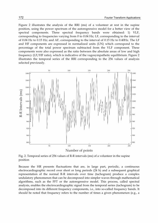
Fourier Transform Applications
172
Figure 2 illustrates the analysis of the RRI (ms) of a volunteer at rest in the supine position, using the power spectrum of the autoregressive model for a better view of the spectral components. Three spectral frequency bands were obtained: 1) VLF, corresponding to frequencies varying from 0 to 0.04 Hz; LF, corresponding to the interval of 0.04 Hz to 0.15 Hz; and AF, corresponding to the interval of 0.15 Hz to 0.40Hz. The LF and HF components are expressed in normalized units (UN) which correspond to the percentage of the total power spectrum subtracted from the VLF component. These components were also expressed as the ratio between the absolute areas of low and high frequency (LF/HF ratio), which is indicative of the vagosympathetic equilibrium. Figure 2 illustrates the temporal series of the RRI corresponding to the 256 values of analysis selected previously.
1080
1060
1040
1020
1000
980
960
940
920
900
880
50 100 150 200 250
50 100 150 200 250
Number of points
1080
1060
1040
1020
1000
980
960
940
920
900
880
R-R
Inte
rval
s (m
s)
Fig. 2. Temporal series of 256 values of R-R intervals (ms) of a volunteer in the supine position
Because the HR presents fluctuations that are, in large part, periodic, a continuous electrocardiographic record over short or long periods (24 h) and a subsequent graphical representation of the normal R-R intervals over time (tachogram) produce a complex undulatory phenomenon that can be decomposed into simpler waves through mathematical algorithms, such as the FFT or the autoregressive model. This process, called spectral analysis, enables the electrocardiographic signal from the temporal series (tachogram) to be decomposed into its different frequency components, i.e., into so-called frequency bands. It should be noted that frequency refers to the number of times a given phenomenon (e.g., a

Spectral Analysis of Heart Rate Variability in Women
173
sound wave, electric current or any form of cyclic wave) occurs over time. Normally, the frequency unit employed is Hertz (Hz), which is equivalent to one cycle per second. Figure 3 shows the application of an autoregressive model to view the power spectrum of the analysis of heart rate variability corresponding to these values of a volunteer of this study.
In long records (24 h), the total power is decomposed into four distinct bands: 1) high frequency band (HF), oscillating at a frequency of 0.15 a 0.40 Hz, i.e., 9-24 cycles/min, corresponding to the heart rate variations related to the respiratory cycle (respiratory sinus arrhythmia), which are typically modulated by parasympathetic activity; 2) low frequency or LF band (0.04 to 0.15 Hz or 2.4 to 9 cycles/min), modulated by both sympathetic and parasympathetic activities, with a predominance of sympathetic in some specific situations, and which reflects the oscillations of the baroreceptors system; 3) very low frequency or VLF band (0.003 to 0.04 Hz or 0.2 to 2.4 cycles/min), depending on the thermoregulatory mechanisms and the renin-angiotensin system, which is also regulated by sympathetic and parasympathetic activities; and 4) ultra low frequency or ULF band (< 0.003 Hz or < 0.2 cycles/min), which corresponds to most of the total variance, but whose physiological significance is not yet well defined. This band is influenced by the parasympathetic and sympathetic systems and is obviously absent from short duration records. It appears to be related with the neuroendocrine system, circadian rhythm, and other systems (Task Force, 1996).
A high frequency component equivalent to 0.25 Hz (15 cycles/min = 15 cycles/60 s = 0.25 cycles/s = 0.25 Hz), a low frequency component equivalent to 0.1 Hz (6 cycles/min) and a very low frequency component of 0.016 Hz (1 cycle/min). The combination of these three sine waves generates a complex wave signal that can be compared to the signal obtained when the heart rate is expressed on a temporal graph (tachogram). Moreover, the calculation of the area covered by each frequency band (which is proportional to the square of the amplitude of the original signal and hence, in this case, is expressed in ms2) enables one to separate the amount of variance (power) ascribed to each frequency. This allows for a more detailed study of the individual participation of each of the divisions of the ANS (sympathetic and parasympathetic) in different physiological and pathological situations, as well as its relationship with the main systems that interfere with HRV (respiratory, vasomotor, thermoregulatory, renin-angiotensin and central nervous systems). In fact, this is the main difference between spectral analysis and time domain analysis, since the latter generally fails to distinguish the dominant rhythms or oscillations that give the heart rate its variability (Task Force, 1996).
Spectral components are usually measured in absolute values of power (ms2). However, the values of LF and HF can also be expressed in normalized units (nu), which represent the value of each of these components in relation to the total power (TP) minus the VLF component. These values are calculated by means of the following formulas: HF (nu) = HF/(TP – VLF) x 100 and LF (nu) = LF/(TP – VLF) x 100. This minimizes the effects of changes in the VLF range on the other two components with faster frequencies (LF and HF). Another frequently used measure is the LF/HF ratio, which can provide useful information about the balance between the sympathetic and parasympathetic systems. It should also be noted that, because absolute values in ms2 are highly variable and distributed asymmetrically, they usually require logarithmic transformation (Task Force, 1996).

Fourier Transform Applications
174
150
100
50
0
Pow
er s
pect
ral d
ensi
ty (m
s )2
0 0.1 0.2 0.3 0.4 0.5 0.6 0.7
Frequency (Hz) Fig. 3. Power spectrum of the analysis of HRV obtained by applying an autoregressive model to a dataset of 256 values of R-R intervals in the supine position from one of the volunteers of this study, showing the VLF (light gray), LF (medium gray) and HF (dark gray) bands
4. Heart rate variability and oral contraceptives Third-generation combined oral contraceptives (COCs) containing desogestrel and gestodene (GEST) were introduced to reduce adverse effects such as fluid retention, nausea, headaches, and weight changes (Arangino et al., 1998; Read, 2010). The balance of risks and benefits of COC use varies, depending on patterns of usage and background risk of disease (Hannaford et al., 2010). The repercussions of COCs on cardiac autonomic modulation have not yet been thoroughly investigated. Studies reveal that female sex hormones influence cardiovascular autonomic function (Minson et al., 2000; Neves et al., 2007; Carter et al., 2009). Leicht et al. (2003) reported a positive correlation between circulating estrogen levels and HRV.
Furthermore, the cardioprotective effects of endogenous estrogen through vasodilation and inhibition of blood vessel injuries have been reported (Mendelsohn & Karas, 1999). Low levels of estrogen are associated with a reduction of cardiac autonomic modulation (Moodithaya 2009). Large clinical trials have shown that the long-term use of estrogen in combination with a progestogen may not be beneficial, and could even compromise the efficiency of autonomic HR modulation. Minson et al. (2000) confirmed that COC use can modify baroreflex sensitivity and sympathetic activity. However, Santos et al. (2008) and Schueller et al. (2006) found that COC users and non-users showed similar HRV indices.

Spectral Analysis of Heart Rate Variability in Women
175
Carter et al. (2009) observed no effects of OC use on the sympathetic modulation of the heart during orthostatic stress, nor differences in that regard between the phase of intake of active pills and that of intake of inactive pills. Women with greater physical activity, both users and non-users of OCs, showed a predominance of parasympathetic modulation and presented a greater complexity of pattern distribution and less regularity and predictability of sequential patterns than sedentary groups. Wenner et al. (2006) evaluated amenorrheic and eumenorrheic athletes who were users and non-users of OCs, and observed no influence on cardiac autonomic function. However, other studies suggest that there is a relationship between OC use and autonomic HR modulation, which the authors attribute to changes in vagal peripheral modulation caused by high levels of circulating estrogen (Minson, 2000; Leicht et al., 2003).
Santos et al. (2008) analyzed the autonomic modulation of HR based on frequency domain (LF, HF and LF/HF) indices and found that the use of contraceptives did not affect the results, since they detected no difference among the groups under study. This finding may be attributed to the pharmacological properties of low estrogen/progesterone dosages, as well as to the maintenance of the integrity of the autonomic modulation of HR, since the values found here fall within the range of normality. The results of this study suggest that low estrogen/progesterone dosages do not impair autonomic modulation in the age group under study.
5. Heart rate variability and hormonal therapy The aging process causes changes in the autonomic modulation of the cardiovascular system, and particularly in HR. The literature reports that parasympathetic activity in the sinus node decreases with age, leading to a reduction in HRV and a greater risk for cardiovascular events (Lipsitz et al., 1990). Structural and functional changes in the blood vessels, in the cardiac conduction system and in the sensitivity of baroreceptors, as well as increased myocardial stiffness, leading to greater force of contraction and reduced ventricular filling, contribute to reduce the functional capacity of the cardiovascular and hemodynamic system (Walsh, 1987). In addition, with increasing age, submaximal physical activity and decline in functional capacity lead to increased physiological stress (Perini et al., 2002).
The incidence of cardiovascular diseases among premenopausal women is low when compared to that of men in the same age group, but increases significantly after this period (Gensini et al., 1996). In several countries, cardiovascular diseases are the major cause of morbidity and mortality among postmenopausal women, representing an important public health problem (Mosca et al., 1997). The increase in the incidence of cardiovascular events among middle-aged women has been associated with the hypoestrogenism typical of this period of women’s lives (Greendale et al., 1999).
With regard to autonomic heart function, some studies have demonstrated the harmful effects of hypoestrogenism on HRV. Mercuro et al. (2000) found a reduction in HRV indices, analyzed in the time and frequency domains, after bilateral oophorectomy, i.e., through the interruption of estrogen production, as occurs in menopause. Liu et al. (2003) demonstrated higher values of HRV, analyzed in the time domain, in premenopausal

Fourier Transform Applications
176
women than in postmenopausal women and men in the same age group, illustrating the importance of estrogens in the autonomic differences brought about by menopause. Similar findings, also analyzed in the time domain, were reported by Brockbank et al. (2000) for premenopausal women compared to women after more than one year of menopause. Davy et al. (1998) reported that young women have higher HRV than menopausal women, and that HRV in both active and sedentary women tends to decline with advancing age. In earlier studies conducted in our laboratory (Ribeiro et al., 2001; Neves et al., 2007), lower levels of HRV in menopausal women compared to young women were also recorded.
To ascertain if a physical training program could promote physiological adaptations and improved sympathovagal balance of the heart, attenuating the deleterious effects of menopause on the cardiovascular system, Sakabe (2007) evaluated 18 sedentary women divided into two groups: Control Group – 10 postmenopausal women (50 to 60 years old) without hormone therapy (HT); and HT Group – 8 postmenopausal women (50 to 60 years old) undergoing HT (estradiol plus levonorgestrel). Both groups were assessed at two different times: before (assessment) and after (reassessment) a 3-month physical training program (PTP). Protocol 1 – to evaluate the autonomic modulation of the HR, the HR was recorded under resting conditions, supine and sitting positions, for 15 minutes in each position. The indices evaluated in Protocol 1 were: mean HR and R-R intervals (RRI), RMSSD index of the RRI, low (LF) and high (HF) frequency bands of the spectral analysis, in normalized units, and LF/HF ratio. It was concluded that hormone replacement therapy did not have a significant effect on HRV.
6. Heart rate variability and menopause Postmenopausal women have greater sympathetic and less parasympathetic activity than premenopausal women (Brockbank et al., 2000; Earnest et al., 2010). Moreover, Mercuro et al.’s study (2000) reveals the harmful effects of hypoestrogenism on the autonomic modulation of the HR, while other studies have demonstrated numerous evidences that endogenous hormones (estrogen and progesterone) contribute to a cardioprotective phenotype in women (Vitale et al., 2009).
Parasympathetic modulation shifts to a lower range with normal aging. Although parasympathetic modulation is generally higher in women than men, aging reduces the difference between genders, with changes in HRV beginning approximately at menopause (Earnest et al., 2010). Boettger (2010) examined changes in cardiovascular autonomic parameters obtained from short-term recordings over time. The data he collected indicated a lifelong shift in autonomic balance toward sympathetic predominance, starting at the age of 30 years.
Zuttin (2009) evaluated and compared autonomic modulation of the HR at rest in healthy young, premenopausal and postmenopausal women leading a sedentary lifestyle, to verify cardiovascular adjustment in response to postural changes. This investigation involved 113 healthy sedentary women, who were divided into a young group (YG) with an average age of 23±3.4 years (n=40), a premenopausal group (PreMG) aged 36±3.1 years (n= 39), and a postmenopausal group (PostMG) with an average age of 55±4.5 years (n=34).

Spectral Analysis of Heart Rate Variability in Women
177
In the supine position, it was found that the YG presented significantly higher values of the HF index in absolute units (ms2) and lower LF values (ms2) and ratio than the PostMG. In addition, the YG and PostMG showed a statistical difference in all the evaluated indices (p<0.05), while no difference was found between the PreMG and PostMG groups (p>0.05). In a comparison of the YG vs. PreMG and YG vs. PostMG groups in the sitting position, the YG presented significantly higher values for the ratio (p<0.05).
With regard to the effect of postural adjustment on the autonomic HR modulation, a comparison of the indices obtained in the supine and sitting positions revealed significant differences (p<0.05) in all the indices. On the other hand, the PreMG groups showed a difference in the LF/HF index (p<0.05), while the PostMG group showed no significant difference (p<0.05).
Having calculated the regression coefficients, it was found that the straight line of the adjusted regression indicates that, as the age of the subjects increases, it is possible to estimate the reduction of the HF index (ms2). The parameters indicate mainly a reduction of the postural change in parasympathetic modulation. With aging, the adjustment capacity diminishes, as indicated by the delta between the supine and sitting positions.
7. Conclusions This chapter discussed the measurement and analysis of HRV, as well as results of data for women and the relationship between aging, hormonal changes (oral contraceptives and hormone replacement therapy) which contribute to modifications in the autonomic control of heart rate.
8. Acknowledgments This chapter was financed by the Brazilian research funding agencies CNPq (National Council for Scientific and Technological Development – Process no. 370448/2007-3) and FAPESP (São Paulo Research Foundation – Process no. 2006/56788-1).
9. References Akselrod, S. (1995). Components of heart rate variability: Basic Studies. In: Heart Rate
Variability Malik, M & Camm, AJ, (Ed.), pp. 147-163, Futura Publishing Company, New York.
Arangino, S. et al. (1998). Effect of desogestrel-containing oral contraceptives on vascular reactivity and catecholamine levels. Contraception, Vol. 58, pp. 289 – 93, ISSN 1879-0518 (Electronic).
Boettger, M. K. et al. (2010). Influence of Age on Linear and Nonlinear Measures of Autonomic Cardiovascular Modulation. Annals Noninvasive Electrocardiology, Vol. 15, No. 2, pp. 165–174., ISSN 1542-474X (Electronic).
Brockbank, C. L. et al. (2000). Heart rate and its variability change after the menopause. Experimental Physiology, Vol. 85, No. 3, pp. 327-330, ISSN 1469-445X (Electronic).
Fourier Transform Applications
178
Carter, J. B., Banister, E. W. & Blaber, A. P. (2003). The effect of age and gender on heart rate variability after endurance training. Medicine and Science in Sports and Exercise, Vol. 35, No. 8, pp. 1333-1340, ISSN 1530-0315 (Electronic).
Catai, A. M. et al. (2002). Effects of aerobic exercise training on heart rate variability during wakefulness and sleep and cardiorespiratory responses of young and middle-aged healthy men. Brazilian Journal of Medical and Biology Research, Vol. 35, pp. 741–752, ISSN 1414-431X (Electronic).
Collier, S. R. (2008). Sex differences in the effects of aerobic and anaerobic exercise on blood pressure and arterial stiffness. Gender Medicine, Vol.5, No. 2, pp. 115-123, ISSN 1878-7398 (Electronic).
Davy, K. P. et al. (1998). Elevated heart rate variability in physically active young and older adult women. Clinical Science, Vol. 94, No. 6, pp. 579-584, ISSN 1470-8736 (Electronic).
Earnest, C. et al. (2010). Autonomic function and change in insulin for exercising postmenopausal women. Maturitas, Vol. 65, No. 3, pp. 284–291, ISSN 1873-4111 (Electronic).
Eckberg, M. D. (1997). Sympathovagal Balance: a critical appraisal. Circulation, Vol. 96, No. 9, pp. 3224-32, ISSN 1524-4539 (Electronic).
Gensini, G. F. et al. (1996). Menopause and risk of cardiovascular disease. Thrombosis Research, Vol. 84, No. 1, pp. 1-19, ISSN 1879-2472 (Electronic).
Greendale, G. A., Lee, N. P. & Arriola, E. R. (1999). The menopause. Lancet, Vol. 353, No. 9152, pp. 571-580, ISSN 1474-547X (Electronic).
Hainsworth (1998). Physiology of the cardiac autonomic system. In: Clinical guide to cardiac autonomic tests, Malik, M., (Ed.), pp. 51-65. Kluwer Academic Publishers, Dordrecht, Boston, London.
Hannaford, P. C. et al. (2010). Mortality among contraceptive pill users: Cohort evidence from Royal College of General Practitioners’ Oral Contraception Study. British medical journal, Vol. 340, pp. c927, ISSN 1468-5833 (Electronic).
Leicht, A.S., Hirning, D. A. & Allen, G. D. (2003). Heart rate variability and endogenous sex hormones during the menstrual cycle in young women. Experimental Physiology, Vol. 3, pp. 441-446, ISSN 1469-445X (Electronic).
Lipsitz, L. A. et al. (1990). Spectral characteristics of heart rate variability before and during postural tilt. Relations to aging and risk of syncope. Circulation, Vol. 81, pp. 1803–1810, ISSN 1524-4539 (Electronic).
Liu, C. C., Kuo, T. B., Yang, C. C. (2003). Effects of estrogen on gender-related autonomic differences in humans. American Journal of Physiology-Heart and Circulation Physiology, Vol. 285, No. 5, pp. 2188-2193, ISSN 1522-1539 (Electronic).
Longo, D. F. & Correia, M. J. (1995). Variabilidade da frequência cardíaca. Revista Portuguesa de Cardiologia, Vol. 14, pp. 241-262, ISSN 0870-2551.
Melo, et al. (2005). Effects of age and physical activity on the autonomic control of heart rate in healthy men. Brazilian Journal of Medical and Biological Research, Vol. 38, n. 9, p. 1331-1338, ISSN 1414-431X (Electronic).
Mendelsohn, M. E. & Karas, R. H. (1999). The protective effects of estrogen on the cardiovascular system. New England Journal of Medicine, Vol. 340, pp. 1801-1811, ISSN 1533-4406 (Electronic).
Spectral Analysis of Heart Rate Variability in Women
179
Mercuro, G. et al. (2000). Evidence of a role of endogenous estrogen in the modulation of autonomic nervous system. American Journal of Cardiology, Vol. 85, pp. 787-789, ISSN 1879-1913 (Electronic).
Minson et al. (2000). Sympathetic activity and baroreflex sensitivity in young women taking oral contraceptives. Circulation, Vol. 102, pp. 1473 – 1476, ISSN 1524-4539 (Electronic).
Moodithaya, S. S. & Avadhany, S. T. (2009). Comparison of cardiac autonomic activity between pre and post menopausal women using heart rate variability. Indian Journal of Physiology and Pharmacology, Vol. 53, pp. 227 – 234, ISSN 0019-5499 (Print).
Mosca L, et al. (1997). Cardiovascular disease in women: a statement for healthcare professionals from the American Heart Association. Writing Group. Circulation, Vol. 96, No. 7, pp. 2468-2482, ISSN 1524-4539 (Electronic).
Neves, V. F. C, et al. (2007). Autonomic modulation of heart rate of young and postmenopausal women undergoing estrogen therapy. Brazilian Journal of Medical and Biological Research, Vol. 40, pp. 491-499, ISSN 1414-431X (Electronic).
Perini, R. et al. (2002). Aerobic training and cardiovascular responses at rest and during exercise in older men and women. Medicine and Science in Sports and Exercise, Vol. 34, No. 4, pp. 700-708, ISSN 1530-0315 (Electronic).
Read, C. M. (2010). New regimens with combined oral contraceptive pills-moving away from traditional 21/7 cycles. European Journal of Contraception and Reproductive Health Care, Vol. 15, No. 2, pp. 32-41, ISSN 1473-0782 (Electronic).
Ribeiro, T. F. et al. (2001). Heart rate variability under resting conditions in postmenopausal and young women. Brazilian Journal of Medical and Biological Research, Vol. 34, No. 7, pp. 871-877, ISSN 1414-431X (Electronic).
Sakabe, D. W. (2007). Efeitos do treinamento físico sobre a modulação autonômica da frequência cardíaca e a capacidade aeróbia de mulheres pós-menopausa sem o uso de terapia hormonal, pp. 1-170, Avariable from:
http://www.teses.usp.br/teses/disponiveis/17/17145/tde-21052008-135005/pt-br.php
Santos, M. C. S. et al. (2008). Influence of oral contraceptive use on lipid levels and cardiorespiratory responses among healthy sedentary women. Brazilian Journal of Physical Therapy, Vol. 12, pp. 188 – 94, ISSN 1413-3555.
Schueller, P. O. et al. (2006). Effects of synthetic progestagens on autonomic tone, neurohormones and C-reactive protein levels in young healthy females of reproductive age. International Journal of Cardiology, Vol. 111, pp. 42 – 48, ISSN 1874-1754 (Electronic).
Silva, E et al. (1994). Design of a computerized system to evaluate the cardiac function during dynamic exercise. Physics in Medicine & Biology, Vol. 33, p. 409 abstract.
Task Force of the European Society of Cardiology and the North American Society of Pacing and Electrophysiology (1996). Heart rate variability: standards of measurements, physiological interpretation, and clinical use. Circulation, Vol. 93, pp. 1043-1065, ISSN 1524-4539 (Electronic).
Vitale, C., Mendelsohn, M. E. & Rosano, G. M. C. (2009). Gender differences in the cardiovascular effect of sex hormones. Nature Reviews. Cardiology, Vol. 6, pp. 532–542.

Fourier Transform Applications
180
Walsh, R. A. (1987). Cardiovascular effects of the aging process. The American Journal of Medicine, Vol. 82, No,1B, pp. 34-40, ISSN 1555-7162 (Electronic).
Wenner, M. M. et al. (2006). Preserved autonomic function in amenorrheic athletes. Journal of Applied Physiology, Vol. 101, pp. 590 –597, ISSN 0021-8987 (Print).
Zuttin, R. Z. (2009). Influência da idade sobre a modulação autonômica da frequência cardíaca e a capacidade aeróbia em mulheres. pp. 1-90, Piracicaba, Brazil, Available from https://www.unimep.br/phpg/bibdig/aluno/visualiza.php?cod=528.

0
Cortical Specification of a Fast FourierTransform Supports a Convolution
Model of Visual Perception
Phillip SheridanGriffith University
Australia
1. Introduction
Currently, the full extent of the role Fourier analysis plays in biological vision is unclear.Although we have examples of sensory organs that perform Fourier transforms, e.g. the lensof the eye and the cochlear, to date there is no direct empirical evidence for its implementationin cortical architecture. However, there does exist intriguing theoretical evidence that suggestsa role for the Fourier transform in a primate’s primary visual cortex (area V1) which emergesfrom recent developments in our knowledge of contextual modulation. This paper proposes anew Fourier transform and a specification of how this transform has a natural implementationin cortical architecture. The significance of this new Fourier transform and its specificationin neural circuitry is that it provides a plausible explanation for previously unexplainedobservable properties of the primate vision system.
1.0.0.1
The spatial response properties, such as orientation tuning and spatial frequency tuning,of neurons in area V1 have been known for some time (Schiller et al., 1976). For awhile, it was generally accepted that these tuning functions of receptive fields are largelycontext-independent (De Valois et al., 1979). However, later research has demonstratedcontextual influences from the region close to the receptive field (Sceniak et al., 2001);(Cavanaugh et al., 2002); (Bair & Movshen, 2004). Moreover, it has been found that this nearsurround region of a receptive field can modify receptive field responses through suppression(Blakemore & Tobin, 1972) and by cross-orientation facilitation effects (Sillito & Jones, 1996);(Cavanaugh et al., 2002); (Kimura & Ohzawa, 2009). It has also been demonstrated thatlong-range contextual modulation is as robust a feature of neural function in area V1 as theextensively studied receptive field properties of this area (Lamme, 1995). Since that time, theevidence for long-range contextual modulation continues to grow, e.g. (Zipser et al., 1996);(Lamme et al., 1998); (Lee et al., 1998).
1.0.0.2
Concurrent with this research establishing the empirical evidence for contextual modulationhas been research aimed at developing functional models of V1 that are consistent withthe empirical evidence. In the early 1980’s the concept of convolution was employed byDavid Marr (Marr & Hildreth, 1980) as a model that accounted for considerable observable
7
2 Will-be-set-by-IN-TECH
properties of the human vision system. Since that time further theoretical and empiricalevidence has been mounting that supports such a model. In particular, it has been shownthat response properties of neurons in area V1 are modeled by convolution of the input imagewith a family of Gabor functions (Sanger, 1988). Further research has demonstrated that theupper layers of area V1 are modeled well by a bank of Gabor filters (Grigorescu et al., 2003);(Huang et al., 2008); (Lee & Choe, 2003); (Ursine et al., 2004); (Tang et al., 2007). A related, butalternative, approach to the Gabor response functions to model simple and complex cells ofV1 is the use of Gaussian derivatives (Huang et al., 2009). The common denominator of thesecontextual modulation models is long-range convolution. However, the issue of acceptingthese state of the art computational models of contextual modulation as plausible functionalmodels of Layer 2/3 of V1 thus becomes one of addressing the cortical convolution conundrum,more specifically: how are the large scale convolutions required by such models accountedfor in cortical architecture?
1.0.0.3
This paper’s goal is to address the cortical convolution conundrum. In the process, we willpropose a new fast Fourier transform, named Generalised Overarching SHIA Fast FourierTransform (GOSH-FFT) and argue:
• GOSH-FFT has a natural implementation in the cortical architecture of visual area V1, and
• Its implementation provides a plausible cortical mechanism to account for theconvolutions implied by long-range contextual modulation.
The rest of this paper is organised as follows: Section 2 provides a description of keyneurophysiological and mathematical concepts underpinning the main thrust of this paper.Section 3 describes the Generalised Overarching SHIA Fast Fourier Transform (GOSH-FFT).Section 4 proposes a new interpretation of the physiology of long-range intrinsic connectionsand reinterprets previously introduced physiological concepts to propose a plausible corticalimplementation of GOSH-FFT. Section 5 discusses various implications of the novel materialof this paper. Section 6 summarises and concludes the paper. Section 7 is an appendix thatcontains a MatLab-like pseudo-code description of GOSH-FFT and a mathematical proof ofGOSH-FFT.
2. Background
This section reviews neurophysiological and mathematical concepts pertinent to theunderstanding of GOSH-FFT and its cortical implementation.
2.1 Physiological background
The primary visual cortex (V1) has a distinctive layer structure. Inputs from the lateralgeniculate nucleus (LGN) of the thalamus arrive chiefly to layer 4 in the monkey (Fitzpatricket al., 1985). Layers 2/3 of monkey V1 contain the first neurons in the feedforward hierarchythat are strongly responsive to orientated stimuli (Schiller et al., 1976); (De Valois et al.,1979); (Parker & Hawken, 1988); (Leventhal et al., 1995). Central to understanding responseproperties of neurons in V1 is the notion of the receptive field (Hubel & Wiesel, 1962). Thereceptive field of a neuron is that region of its visual field to which it responds most strongly.Neurons within layers 2/3 V1 have receptive fields that are oriented. That is, they preferstimuli that are lines of a certain orientation, or oriented texture elements (Hubel & Wiesel,
182 Fourier Transform Applications

Cortical Specification of a Fast Fourier Transform Supports a Convolution Model of Visual Perception 3
1974). The spatial and temporal frequency tuning preferences of neurons in V1 can alsobe measured. The neuron’s response properties measured via the receptive fields resemblespatially localized filters with a preferred orientation and spatial frequency (Schiller et al.,1976); (Foster et al., 1985); (Mikami et al., 1986); (Edwards et al., 1995) or spatio-temporalenergy (Basole et al., 2003); (Basole et al., 2006).
2.1.0.4
The orientation preference of neurons can be mapped using optical imaging techniques andneurological studies, which show good agreement with single cell measurements (Blasdel,1992); and groups of neurons which act as a single unit. It has been experimentallyshown that this single unit activity of large groups of single cells are composed of 104
(first order approximation) interconnected cells even in one local V1 column (Siegel, 1990).The advantages of modeling large scale neuron activity which exhibit cohort macroscopicorganisation was shown by (Sirovitch et al., 1996). No model was presented but organisingprinciples for analyzing and viewing data were presented. These techniques have revealedan intricate structure to the orientation preference map in layers 2/3. A critical feature ofthese structures is the orientation pinwheel (local map), in which the orientation preference ofthe neuronal population changes through the entire range of 180 degrees of orientations overthe 360 degrees of polar range of the circular pinwheel. At the centre of the pinwheel is thesingularity, which is the point at which lines of iso-orientation preference meet (Obermayer &Blasdel, 1993).
2.1.0.5
The cortex is often called the iso-cortex because of the repeated structures of which it iscomprised (Douglas & Martin, 1991). The smallest scale of structure is the minicolumn which,in the monkey, consists of 30 adjacent pyramidal cell shafts in layers 2/3 packed within adiameter of 23 μm (Peters & Sethares, 1996). There are approximately 20 cell bodies within aminicolumn in layers 2/3. The next largest physical scale in V1 at which repeated structuresoccur is the cortical column (Lund et al., 2003). The cortical column is 200 μm in diameter andis the scale at which long-range patchy connections terminate. A number of anatomical andfunctional markers repeat at a larger scale of 400 μm. These include the distance betweenCO blobs, the approximate periodicity of the orientation preference map, and the spatialscale of a single ocular dominance band (Lund et al., 2003). Orientation pinwheels are alsoof approximately this spatial scale. Each of these functional markers has been shown to beclosely related to the system of patchy connections, in which like response preference connectsto like, and the inter-patch distance in V1 has this same periodicity of 400 μm (Bartfeld &Grinvald, 1992); (Malach et al., 1993); (Bosking et al., 1997). The largest spatial scale is V1 itself,which is some 4 cm wide in the monkey. There are of the order of 10,000 CO blobs in layers2/3 of V1 (Murphy et al., 1998), and ocular dominance bands of 120 in number (Horton &Hocking, 1998), suggesting that the multiple response property maps with periodicity of 400μm repeat around 10,000 times over layers 2/3 of V1. The input connections from the LGNarborize at a range of scales within layer 4C of V1. These inputs are arranged in block-likestructures at the approximate scale of an ocular dominance band in layer 4C, but at a finerscale of approximately one column in layer 4C (Fitzpatrick et al., 1985). Further fine scalearborizations occur at approximately the scale of one minicolumn in layer 4A. At the globalscale of the cortex, inputs from the LGN are organized into a retinotopic mapping of thevisual field (Rolls and Cowey 1970; (Tootell et al., 1988). Connectivity into the layers 2/3
183Cortical Specification of a Fast FourierTransform Supports a Convolution Model of Visual Perception
4 Will-be-set-by-IN-TECH
of V1 occurs via a number of anatomical routes, apart from the well described feedforwardconnections from layer 4 (Fitzpatrick et al., 1985). Other routes of information transfer includeextra-striate feedback (Rockland et al., 1994); (Rockland & Vanhoesen, 1994); (Angelucci et al.,2002), long-range intrinsic fibres within V1 (Blasdel et al., 1985), as well as feedback from V1to the lateral geniculate nucleus (Marrocco et al., 1982); (Briggs & Usrey, 2007), and diffusionof visual signal in the retina (Kruger et al., 1975); (Berry et al., 1999).
2.1.0.6
The finest scale of axonal projections within V1 are the short-range intrinsic connections thatprovide connectivity between neurons up to the range approximated by an ocular dominancecolumn width, or 400 μm. Within V1, long-range patchy connections extend for 3 mmwithin the supra-granular layers (Stettler et al., 2002) and long-range connections within theinfra-granular layers extend for up to 6 mm (Rockland & Knutson, 2001). V1 also receivesfeedback from at least nine extra-striate areas (Rockland & Vanhoesen, 1994). Extra-striatefeedback is considered by most researchers to be the primary source of long-range horizontalinteractions measured in V1 (Alexander & Wright, 2006). These feedback connections are fastconducting myelinated cortico-cortical fibres, and while they traverse distances of up to 10 cmin the monkey, the transmission delays are of the same order as intrinsic short and long-rangeaxons within V1 (Bringuier et al., 1999); (Girard et al., 2001). These feedback connections areoften in register with the intrinsic patchy system within V1, depending on the area of origin(Angelucci et al., 2002); (Lund et al., 2003). The middle temporal (MT) visual area will servehere as brief illustration of the role of extra-striate feedback in V1. Receptive field sizes inMT are about 10 times larger than in V1 at all eccentricities (Albright & Desimone, 1987).Small focal injections of tracer into V1 indicate that the sizes of the feedback fields from MTto V1 are 21-fold larger than the aggregate receptive size of the V1 injection sites (Angelucciet al., 2002). These feedback connections are an obvious substrate for the integration of globalsignals into V1 (Bullier, 2001). The local-global map hypothesis (Alexander et al., 2004) ofV1 posits a non-local influence on the structure of local maps in V1. This hypothesis statesthat the global visual map in V1 is remapped to the local map scale in V1 in the form of amap of response properties, e.g. orientation, and in the case of the monkey, spatial frequencypreference and colour selectivity. These local maps tile the surface of V1 and each receiveinputs from a large extent of the visual field. So rather than the local map being simply a mapof primitive visual features that apply to a point in visual space, the local map is a map of primitivevisual features as they arise in the organisation of the visual field and become relevant to a location invisual space. As the maximum range of contextual modulation in V1 approaches the size of thevisual field (Alexander & Wright, 2006), the local organisation of response properties can beinfluenced by the functional properties of the global visual field.
2.2 Mathematical background
Fundamental to the Fourier transform proposed in this paper is the Spiral Honeycomb ImageAlgebra (SHIA). This is a data structure that embodies important properties of the naturalvisual constraints imposed by the primate eye (Sheridan et al., 2000). In particular, SHIAhas a discrete, finite and bounded domain which mimics the distribution of photo receptorson the retinal field. The underlying geometry of the SHIA is a hexagonal or rectangularlattice. In the former case, each hexagon has a designated positive integer address expressedin base seven. The numbered hexagons form clusters of super-hexagons of size 7n. These
184 Fourier Transform Applications

Cortical Specification of a Fast Fourier Transform Supports a Convolution Model of Visual Perception 5
self-similar super-hexagons tile the plane in a recursively modular manner. As an example, asuper-hexagon of size 72 = 49 and its concomitant addressing scheme is displayed in Fig. 1 (a).
(a) Hexagonal SHIA
(b) Rectangular SHIA
Fig. 1. Displays the two-level addressing scheme of SHIA: (a) Hexagonal and (b) Rectangular.
In the latter case, each rectangle has a designated positive integer address expressed in basefive. An example of this addressing scheme is displayed in Fig. 1 (b).
185Cortical Specification of a Fast FourierTransform Supports a Convolution Model of Visual Perception

6 Will-be-set-by-IN-TECH
2.2.0.7
The importance of the SHIA addressing scheme is that it facilitates primitive imagetransformations of translation, rotation and scaling. One of these transformations that hasproven to be of particular relevance to the Fourier transform is one that provides rotation andscaling. It is referred to as mapping M10 in the notation of SHIA. Fig. 2 (a) displays an imagerepresented in a four level SHIA, size is 74 = 2401. Fig. 2 (b) represents the effect of applyingM102 = M100 to this image.
The critical observation to make in regard to the effect of M10 is that it produces multiple’near’ copies at reduced resolution of the input image. This transform will play a critical rolein the proposed FFT.
2.2.0.8
The origin of what is now called a Fourier transform dates back to 1807 when Jean BaptisteJoseph Fourier defined the notion of representing a function as a trigonometric series. Thediscrete version of a Fourier transform (DFT) for a one-dimensional signal is defined as:
F(u) =1N
N−1
∑x=0
f (x)e−j2πux/N (1)
for u = 0, ...N − 1, where f (x) is a real valued function, N represents the number of elementsin the signal and j2 = −1.
The effect of this transform is to capture the spatial relationships inherent in the signal f(x)and express these relationships as the sum of sinusoidal function (frequency components).Similarly, the discrete version of an inverse Fourier transform (IDFT) for a one-dimensionalsignal is defined as:
f (x) =N−1
∑u=0
F(x)ej2πux/N (2)
for x = 0, ...N − 1, where F(u) is the Fourier transform of the real valued function f (x), Nrepresents the number of elements in the signal and j2 = −1.
The effect of this inverse Fourier transform is to take a signal in frequency domain back to thespatial domain.
2.2.0.9
Prior to the invention of the digital computer, the Fourier series was employed as a purelyanalytic tool. However, since that time, the development of a class of computationally efficientalgorithms, known as fast Fourier transforms (FFT), has meant the notion has become a usefulcomputational tool (VanLoan, 1992). One of the most attractive computational properties ofthe FFT is its ability to process signals at higher resolution with a minimal increase in cost tocomplexity. Today, most of us benefit from fast Fourier transforms every day without evenknowing it as these algorithms power a vast range of electronic technology such as digitalcameras and cell phones.
2.2.0.10
The relevance of a fast Fourier transform to this paper is its relationship to the notion ofconvolution. The convolution of two functions f (x) and g(x) is denoted by f (x) ∗ g(x) and
186 Fourier Transform Applications
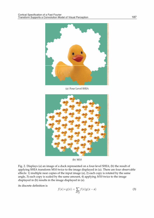
Cortical Specification of a Fast Fourier Transform Supports a Convolution Model of Visual Perception 7
(a) Four Level SHIA
(b) M10
Fig. 2. Displays (a) an image of a duck represented on a four-level SHIA; (b) the result ofapplying SHIA transform M10 twice to the image displayed in (a). There are four observableeffects: 1) multiple near copies of the input image (a), 2) each copy is rotated by the sameangle, 3) each copy is scaled by the same amount, 4) applying M10 twice to the imagedisplayed in (b) results in the image displayed in (a).
its discrete definition isf (x) ∗ g(x) = ∑
a∈gf (x)g(x − a) (3)
187Cortical Specification of a Fast FourierTransform Supports a Convolution Model of Visual Perception

8 Will-be-set-by-IN-TECH
A well known result to researchers in the field of signal processing is the ConvolutionTheorem, which relates convolution in the spatial domain to convolution in the frequencydomain. For two functions, f (x) and g(x), let F(x) and G(x) represent the Fourier transformof f (x) and g(x) respectively. The Convolution Theorem states that,
f (x) ∗ g(x) � F(x)G(x) (4)
In other words, the convolution of two functions in the spatial domain can be achieved by themultiplication of the functions in the frequency domain.
3. Generalised Overarching SHIA fast Fourier transform (GOSH-FFT)
In this section we propose a new fast Fourier transform that, as we will see later, possessesthe potential to be implemented in cortical architecture and thereby address the corticalconvolution conundrum. Associated with SHIA, as described in Section 2.2, is a Cooley-Tuckytype fast Fourier transform, named Generalised Overarching SHIA Fast Fourier Transform(GOSH-FFT). This novel fast Fourier transform employs the transform M10, as describedin Section 2.2, as the critical mechanism that turns a Fourier transform into a fast Fouriertransform.
3.0.0.11
Suppose an image is represented on a SHIA of size 7n, where n ≥ 0. Let m ≥ 0 such thatnmodulom = 0. Let k = n ÷ m and M denote M10m, the composite of M10 ◦ M10 ◦ ... m times.For(i:0:k)
1. Apply M to the input;
2. Perform a discrete Fourier transform over a sequence of sub images of size 7m;
3. Apply the inverse of Mi locally.
A special case of GOSH-FFT was initially described in (Sheridan, 2007), with m = 1. Thesignificance of the initial work was that it demonstrated the intrinsic connection between theFourier transform and primitive image transformations of translation, rotation and scaling. Italso turns out that another special case of GOSH-FFT, when n = 2m, will play a critical role inthe core hypothesis of this paper. This special case, named Particular SHIA FFT (PaSH-FFT),is illustrated in Fig. 3.
A complete statement of Algorithm 3.0.0.11 is written in MatLab-like pseudo-code and canbe found in Section 7 along with a mathematical proof that GOSH-FFT delivers a Fouriertransform.
4. Cortical implementation of contextual modulation
In Section 1, we reviewed state of the art models of contextual modulation and concludedthat these models implied the cortical convolution conundrum. We further motivate thisconundrum by observing that as a consequence of Equation 3, a convolution of the entirevisual field requires every minicolumn in Layer 2/3 of area V1 to receive an input from everyother minicolumn of that layer. As there just are not enough connections to convolve the visualfield in one cortical step, the convolution problem reduces to one of determining, given theknown connectivity, what is the sequence of intermediate neurons an initial input must pass
188 Fourier Transform Applications

Cortical Specification of a Fast Fourier Transform Supports a Convolution Model of Visual Perception 9
(a) Intermediate step (b) Fourier transform
(c) Intermediate step (d) Inverse Fourier transform
Fig. 3. Displays the results of applying the special case of GOSH-FFT, that is PaSH-FFT, toimage of Fig. 2 (a), with n=4 and m=2. The four sub figures display intermediate results ofPaSH-FFT: (a) on completion of first iteration of PaSH-FFT to Fig. 2; (b) Fourier transform oncompletion of second iteration; (c) on completion of first iteration of inverse PaSH-FFT; (d)Inverse PaSH-FFT on completion of second iteration.
through before being output as a convolved value. With the cortical convolution conundrumthus fully formulated, in this section we will establish a specification of a sufficient sequence ofsteps to address the issue. This specification will unfold in three steps. First, we will discusshow the SHIA transform M10 manifests in cortical architecture. We will then employ thismanifestation to demonstrate how neural circuitry accommodates PaSH-FFT. Lastly, we willshow how the cortical manifestation of PaSH-FFT supports long-range convolution.
4.1 Cortical manifestation of M10
A critical component of the fast Fourier transform, PaSH-FFT, is the transform M10.Consequently, it is an imperative of our argument that the redistribution properties of M10 beaccounted for in the neural circuitry of the visual system. To this end we now argue that therequired effects of M10 are accounted for by the long-range properties of patchy connections
189Cortical Specification of a Fast FourierTransform Supports a Convolution Model of Visual Perception

10 Will-be-set-by-IN-TECH
between columns of Layer 2/3 and similarly patchy extra-striate feedback connections to areaV1.
4.1.0.12
It has been argued that the orientation pinwheel comprises a unitary organisational structureor local map in layer 2/3 of area V1 (Hubel & Wiesel, 1974); (Bartfeld & Grinvald, 1992);(Blasdel, 1992). When four pinwheels are reflected about their common borders, a saddlepoint arises at the centre of the four pinwheels. See Fig. 4.
Fig. 4. Displays a schematic diagram of the pinwheel like structures of visual area V1,extracted from Figure 10 page 43 of Bruce et al. (2003).
4.1.0.13
In the macaque, the preferred response properties of V1 neurons can be influenced by activityfrom a wide extent of the visual field. A review of contextual modulation in the monkeydemonstrated contextual modulation in V1 from long-ranges in the visual field (Alexander& Wright, 2006). The review was compiled from a number of experimental paradigms,including visual stimulation with long lines while the neuron’s receptive field is occluded(Fiorani et al., 1992), surround only textures (Rossi et al., 2001) and colour patches placeddistally to the neuron’s receptive field (Wachtler et al., 2003). It was shown that the maximumrange of contextual modulation measurable in V1 approaches a large extent of the visualfield relative to a neuron’s receptive field size or the local cortical magnification factor. Someexperimental paradigms, such as the curve tracing effect (Roelfsema & Lamme, 1998); (Khayatet al., 2004), relative luminance (Kinoshita & Komatsu, 2001), and texture defined boundaries(Lee et al., 1998) show excitatory contextual modulation with ’tuning curves’ that are flat outto the maximum distance tested. The functional connectivity that underlies this long-rangecontextual modulation in the monkey is likely to involve cortico-cortical feedback from highervisual areas working in concert with long-range intrinsic patchy connectivity. In the monkey,the feedback connections to V1 from higher visual areas incorporate inputs from a very largeextent of the visual field (Angelucci et al., 2002); (Lund et al., 2003).
4.1.0.14
In the analysis that follows, the combination of patchy intrinsic connections and patchyfeedback connections are therefore assumed to enable transfer of visual information at rangesapproaching the global scale of the visual field. Moreover, we assume that the quantity anddistribution of these connections are adequate to deliver the effects of transform M10 at thescale of the visual field.
190 Fourier Transform Applications

Cortical Specification of a Fast Fourier Transform Supports a Convolution Model of Visual Perception 11
4.2 Cortical manifestation of PaSH-FFT
The next step in accounting for global convolution in cortical circuitry is to explore howPaSH-FFT manifests itself in cortical architecture. The raw data, at the lowest level ofPaSH-FFT, are complex numbers that must be multiplied and added. The first issue toaddress is to justify our assumption that the operations being performed by a neuroncould be represented as complex arithmetical operations on complex numbers. Specifically,PaSH-FFT requires that a neuron can be regarded as a mechanism capable of representing andmanipulating complex numbers in accordance with the arithmetical operations of additionand multiplication. There are many ways in which to interpret neuronal function in terms ofcomplex addition and multiplication. The model presented by (MacLennan, 1999) is adequatefor the purposes of this paper, where it is shown how the representation of complex numberscan be encoded as the rate and relative phase of axonal impulse. From this encoding, complexmultiplication is associated with the strength of a synaptic connection as the signal passesthrough it and complex addition is associated with the summing of the neuronal inputs.Thus at the lowest level of computation in our model, we assume that the operation beingperformed by a neuron can be represented as complex addition and multiplication.
4.2.0.15
In area V1, each neuron makes use of information available to it in real time. There is evidencethat contextual information is projected to widespread regions in V1 in an anticipatorymanner. Since the spatial changes in the visual field tend to be predictable from previousvisual inputs, anticipatory contextual inputs can arrive in time to be integrated in an adaptivemanner with ongoing feedforward input. In order to express the properties of widespreadcontextual integration in a more formal manner, however, we will use the mathematicalconvenience of assuming that each of the distinct mathematical processes to be describedoccurs in a step-wise fashion. This more constrained approach allows not only each distinctpart of the process to be formulated, but also formulates the inter-relationships betweenthe various sub-processes. Although it is claimed that this approach is appropriate for thepurposes of this paper, it must be acknowledged that the question of how such "contextualintegration" actually occurs in the neuronal system remains open.
4.2.0.16
At the finest scale of connectivity via short-range intrinsic connections, each neuron of alocal map is treated as if it were connected to every other neuron minicolumn of that localmap. While this is not literally true, considerations of poly-synaptic interactions at this localscale, and the real-time, anticipatory nature of visual processing means that it is a reasonableapproximation of the functional connectivity. Consequently, we can assume that each neuronin a local map can sum the outputs of all other neurons in that local map which have beenmultiplied by unique complex numbers. We call such a collection of parallel computations alocal computation. See Fig. 5, which is a schematic diagram of a local computation.
4.2.0.17
This paper now needs to discuss three types of local computations, each of which isdetermined by the interpretation of the input signal and the collection of synaptic strengthswhich weight the input signal. If the input signal is the spatial domain and the weights areassociated with a set of primitive roots of unity, then the resulting local computation is aFourier transform, denoted F. (See Equation 1 for a definition of a Fourier transform.) If the
191Cortical Specification of a Fast FourierTransform Supports a Convolution Model of Visual Perception
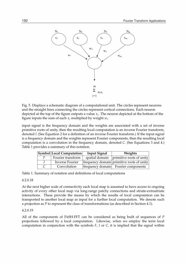
12 Will-be-set-by-IN-TECH
N1 N2 N3 Nm
x1 x2 x3 xm
m
wixi i=1
w1
w3w2
wm
Fig. 5. Displays a schematic diagram of a computational unit. The circles represent neuronsand the straight lines connecting the circles represent cortical connections. Each neurondepicted at the top of the figure outputs a value xi. The neuron depicted at the bottom of thefigure inputs the sum of each xi multiplied by weight wi.
input signal is the frequency domain and the weights are associated with a set of inverseprimitive roots of unity, then the resulting local computation is an inverse Fourier transform,denoted I. (See Equation 2 for a definition of an inverse Fourier transform.) If the input signalis a frequency domain and the weights represent Fourier components, then the resulting localcomputation is a convolution in the frequency domain, denoted C. (See Equations 3 and 4.)Table 1 provides a summary of this notation.
Symbol Local Computation Input Signal WeightsF Fourier transform spatial domain primitive roots of unityI Inverse Fourier frequency domain primitive roots of unityC Convolution frequency domain Fourier components
Table 1. Summary of notation and definitions of local computations
4.2.0.18
At the next higher scale of connectivity each local map is assumed to have access to ongoingactivity of every other local map via long-range patchy connections and striate-extrastriateinteractions. These provide the means by which the results of local computation can betransported to another local map as input for a further local computation. We denote sucha projection as P to represent the class of transformations (as described in Section 4.1).
4.2.0.19
All of the components of PaSH-FFT can be considered as being built of sequences of Pprojections followed by a local computation. Likewise, when we employ the term localcomputation in conjunction with the symbols F, I or C, it is implied that the signal within
192 Fourier Transform Applications

Cortical Specification of a Fast Fourier Transform Supports a Convolution Model of Visual Perception 13
a local map has been sent to every other neuron in that local map through a synapse whosestrength is associated with the appropriate weight of F, I or C respectively.
4.2.0.20
Although it is commonly accepted that the cortex has a massively parallel architecture,currently there exists no comprehensive model to describe these dynamics. The absenceof such a model means that in any particular cortical process, we cannot be sure whichaspects of the process are parallel and which are intrinsically sequential. We will employ thefollowing notation to show how the inherently sequential steps of PaSH-FFT can be mappedinto neural circuitry. Let the symbol � denote the composition of two local computations asfollows: given arbitrary local computations A and B to operate on a signal in sequence let(s)A � B = ((s)A)B.
Note that the operator is to the right of the input signal it operates on, which is enclosed inleft and right parenthesis ().
4.2.0.21
With these concepts in hand, we can now identify the sequential steps of PaSH-FFT. In thisspecial case, the size of the input signal is the square of the size of the local computationand represents two iterations of GOSH-FFT, as described in Section 3. The identification ofthe sequential steps also suggests the sequence of connections that the input signal musttraverse. We now illustrate this with PaSH-FFT, given an input signal s, then the applicationof PaSH-FFT would be expressed as follows:
(s)PaSH − FFT = (s)P � F � P � F � P (5)
Given the assumed neural parallelism, a count of the number of components on the right handside of the equals sign in Equation 5, reveals that a Fourier transform of the entire visual fieldcan be completed by the signal traversing a sequential path connecting five neurons. Likewise,an inverse Fourier transform can be delivered in cortical circuitry as follows:
(s)inversePaSH − FFT = (s)P � I � P � I � P (6)
4.3 Cortical manifestation of convolution
We now progress to the issue of how convolution could be implemented in corticalarchitecture. To this end, we describe the various computational constraints imposed by thecomputational requirements of convolution and argue that the known cortical architecturesatisfies these constraints.
4.3.0.22
The key to the solution of the convolution problem in the neurological domain is provided bythe Convolution Theorem, the same one employed by numerous digital signal processingapplications. This theorem was discussed in Section 2.2. The importance of the theoremis that the convolution of two functions in the spatial domain can be achieved by themultiplication of the functions in the frequency domain. The implications of this theoremto the cortical convolution conundrum are significant. In our model, the components of theFourier transform of the function the input signal is to be convolved with are representedby connection weights. Then, once the input signal has been transformed to the frequency
193Cortical Specification of a Fast FourierTransform Supports a Convolution Model of Visual Perception

14 Will-be-set-by-IN-TECH
domain the required convolutions can be performed by mere multiplications. In corticalterms, each component of the signal, in the frequency domain, must traverse a connection toone more neuron to achieve the desired multiplication. However, the resulting convolution,in the frequency domain, must be transformed back to the spatial domain to complete theconvolution. This is achieved with an inverse Fourier transform. Accordingly, the sequenceof connections along the path that terminates in the output of a convolved value in the spatialdomain is thus given by:
(s)Convolution = (s)P � F � P � F � C � P � I � P � I � P (7)
4.3.0.23
It is assumed that each component of the input signal traverses parallel paths along thenetwork. Thus, the net time cost to complete a convolution is equivalent to the time requiredfor a component of the input signal to traverse a path connecting 10 neurons. This path iscomposed of five short-range intrinsic connections and five long-range connections.
4.4 Analysis
The plausibility of the cortical model of convolution proposed in this paper is fundamentallypredicated on the assumptions made in its formulation. Consequently, we summarise theseassumptions along with the arguments offered to justify them before we provide an analysisof the model’s parameterisation:
1. The number of long-range patchy connections is adequate to achieve a redistribution ofthe global signal via transform M10. This was argued in Section 4.1 and heavily relied ona conclusion based on a review article reported in (Alexander & Wright, 2006).
2. A first order approximation of the number of minicolumns in a local map as 10,000. Thiswas discussed in Section 2.1 and relied on the work reported in (Siegel, 1990).
3. The number of short-range intrinsic connections is adequate to consider each local map asbeing fully connected. This was discussed in Section 4.2 and relied on the work reportedin (Siegel, 1990).
4. A first order approximation of the number of minicolumns in the global map is 10, 0002 =100 million. This was discussed in Section 2.1 and was based on the work reported in(Murphy et al., 1998) and Assumption 2.
4.4.0.24
The first assumption is possibly the most critical as it establishes the fundamental architecturalrelationship between the local and global maps and is essential to PaSH-FFT. The secondtwo assumptions implied that a Fourier transform of the portion of the signal representedin a local map would be completed by each component of the signal traversing one corticalconnection and that on completion of the first iteration of PaSH-FFT, the global signal consistsof 10,000 local discrete Fourier transforms each of which is at the scale of a local map. Then,on completion of the second iteration of PaSH-FFT, the 10,000 local Fourier transforms wouldbe transformed into a global Fourier transform of size 10, 0002 = 100 million, which by thefourth assumption represents the size of the global signal. From this we are able to assertthat the input spatial signal would be transformed to frequency space at a cost of the signaltraversing a path connecting four neurons. With the signal in frequency space, we employed
194 Fourier Transform Applications

Cortical Specification of a Fast Fourier Transform Supports a Convolution Model of Visual Perception 15
the Convolution Theorem to assert that with each component of the global signal traversingone additional connection, the state of the signal would represent a convolved signal infrequency space. This assertion was predicated on the assumption that the weight of eachof these last connections represented the Fourier weight of the appropriate gaussian. The finalstep was to transform the convolved signal back from frequency space to the spatial domain.This was achieved with the inverse PaSH-FFT, which would be completed at the additionalcost of the signal traversing a path connecting a further five neurons. Putting these threesteps together, we arrived at a total path length of 10 connections for the global input signalto be transformed into a representation of global convolution of the visual field. We also notethat this analysis accounted for a single global convolution of the input signal. However,there will be many global convolutions required, possibly up to one for every orientationpreference and spatial frequency preference represented in a local map. Although the inputspatial signal needs only to be transformed into the frequency domain once, each distinctconvolution would require a distinct set of parallel paths to transform the signal back intothe spatial domain. Consequently, the multiple convolutions would not necessarily resultin a longer path. Accordingly, we assert that the transform, PaSH-FFT, with appropriateparameterisation, would deliver a global convolution of the visual field. Moreover, this outputsignal is generated within the required time constraints imposed by observed contextualmodulation. Given our assumptions, the lowest number of iterations required to completea Fourier transform is two. Consequently, 10 represents the length of the shortest path (seeequation 7) possible to deliver a global convolution via PaSH-FFT.
5. Discussion
The signal processing literature describes many different types of fast Fourier transforms(FFT). Although any one of them represents an alternative candidate to PaSH-FFT, theproblem to address is accounting for how they might be implemented within the knownconstraints of cortical architecture. All fast Fourier transforms need to rearrange componentsbetween their intermediate steps of multiply and add. PaSH-FFT derives its rearrangementsof components with the transform M10 that, as argued, is compatible with the distributionand quantity of long-range cortical connections. If any other FFT could be substituted forPaSH-FFT in the model, one would need to account for the rearrangement phase of that FFTwithin the known connectivity of area V1.
5.0.0.25
Another issue worthy of some discussion pertains to the Fourier transform and the absence ofempirical evidence that would irrefutably demonstrate its cortical implementation. Part of theexplanation for this lack of evidence may be provided by the role the Fourier transform playsin the vision process as suggested by this paper. That is, PaSH-FFT was shown to be a meansto an end (convolution), not the end itself. Consequently, the question of finding neuronsthrough empirical experimentation that measures response properties of neurons that closelymodel the profile of a Fourier transform may remain unanswered for some time to come.
5.0.0.26
Underpinning the proposed implementation of PaSH-FFT in cortical architecture is a highlysimplistic model of the parallelism inherent in the cortex. The model employed did nottake into account at least two well accepted features of this parallel architecture. First, thesystem itself somehow synchronises the flow of the signal. Second, the cortex does not
195Cortical Specification of a Fast FourierTransform Supports a Convolution Model of Visual Perception

16 Will-be-set-by-IN-TECH
need computation-like synchronisation or state update. Synchronisation can be provided byconsidering "Small World" relationships. (Gao et al., 2001) have shown that a "Small World"network needs only a small fraction of long-range couplings to obtain a great improvement inboth stochastic resonance and synchronisation in network connectivity of bistable oscillators.We suggest that the known topology of the visual cortex (Zeki, 1993) if considered as a"Small World" network can provide the foregoing benefits. They would be consistent with thelong-range and short-range connectivities of V1 to retinal neurons which have the requiredbistable oscillator condition provided by on-centre or off-centre neurons responses to lightand dark and including those with colour opponency properties. The long and short-rangeselectivity for connections can be dynamic based on the neuron threshold levels and spatialfrequency channels (Dudkin, 1992). The system updates a neuronal state only when newinformation indicates a change in the input signal.
5.0.0.27
The cortical implementation of PaSH-FFT was discussed in Section 4.2 where it was arguedthat the known connectivity of area V1 was sufficient to support its cortical implementation.It was then argued that this implementation could deliver the required convolution in a’small’ number of sequential steps. However, the argument did not rule out the possibilityof an alternative mechanism that would deliver the required convolution in fewer stepsthan PaSH-FFT. It would appear that without a sufficiently developed model of the brain’sparallelism, it is unlikely that a mathematical proof of a lower bound for the minimum numberof sequential steps could be produced. Currently, the only bound that we can be sure of is thatthe required convolution could not be completed in one step. The question of determining theminimum lower bound remains an open question.
5.0.0.28
The role of the frequency domain was at the heart of the solution to the cortical convolutionconundrum proposed in this paper. However, the possibility of performing the convolutionin the spatial domain without resorting to the frequency domain cannot be ruled out by anyargument presented in this paper. Although it is unclear how this could be accomplishedwithout resorting to a highly asymmetric model of the distribution of the connectivity oflong-range connections. In any case, the search for an explanation of how the dynamicreconfiguration implied by the analysis of this paper is actually accomplished is likely toprovide many different conjectures along the way. One possible avenue in this endevourmight be provided by further tracer experiments such as those reported in (Angelucci et al.,2002).
6. Summary and conclusion
This paper reviewed the evidence for long-range contextual modulation and concluded thatit implied cortical convolution at the scale of the visual field. This resulted in the need toaddress the problem of how such long-range convolution could be accounted for with knowncortical connectivity and within known time constraints. The paper proposed a solution tothe problem that emerged from a mathematical analysis of cortical connectivity to account forthe implied constraints of long-range convolution. In particular, it was argued that the knowndistribution of the long-range patchy connections and extrastriate connections is adequateto provide the means by which the global visual signal can be transformed into frequencyspace where the convolution can be performed. The main thrust of the argument was that
196 Fourier Transform Applications

Cortical Specification of a Fast Fourier Transform Supports a Convolution Model of Visual Perception 17
these long-range connections facilitated the transformation of the signal into and out ofthe frequency domain via a new fast Fourier transform named PaSH-FFT. A mathematicalproof of the most general form of this FFT, GOSH-FFT, was provided in the appendix alongwith MatLab-like pseudo-code to facilitate the implementation of GOSH-FFT in computersoftware.
6.0.0.29
It was shown that, to a first order approximation, a cortical implementation of PaSH-FFT couldaccount for the large scale convolution implied by known models of contextual modulation.The significance of PaSH-FFT is that it:
• represents a plausible cortical mechanism to account for long-range contextualmodulation;
• suggests a theoretical explanation of how the brain might be wired to achieve large scaleFourier analysis;
• opens up the possibility of explaining other cortical processes via frequency spacecomputations.
It is the conclusion of this paper that the processing of the visual signal in the frequencydomain via a fast Fourier transform plays a fundamental role in primate vision.
7. Appendix
In this appendix, we present the pseudo-code for GOSH-FFT and a mathematical proof ofGOSH-FFT.
7.1 Appendix A
This section presents a formal statement of GOSH-FFT in MatLab-like pseudo-code.
Notation:
x = Complex array specifying the input signalbase = 7α, where α is an integer greater than zeron = 7β, where β/α , is an integer greater than zero.⊗ denotes scalar multiplication in SHIA
01 function y = GOSH − FFT(x, n, base, α)02 y ← x03 f orlevel = 1 : logbase(n04 f ← m10(y, α)05 r ← rootsO f Unity(baselevel)06 w ← m10(r, α)07 F ← localDFFT( f , w, level, n, base)08 y ← localM10Inverse(F, level, n, base, α)09 r ← w10 end11 end
197Cortical Specification of a Fast FourierTransform Supports a Convolution Model of Visual Perception

18 Will-be-set-by-IN-TECH
01 function T = m10(t, α)02 f ori = 0 : n − 103 a ← convertToSHIA(i)04 b ← 10α ⊗ a05 c ← convertFromSHIA(b)06 T(c) ← t(i)07 end08 end
01 function F = localDFT( f, w, level, n, base )02 subSignalSize ← baselevel
03 numSubSignals ← n/subSignalSize04 f ors = 0 : numSubSignals − 105 tab ← s × subSignalSize06 f ors = 0 : subSignalSize − 107 wLB ← i × base08 lB ← i × base + tab09 uB ← lB + base − 110 f oru = lB : uB11 F(u) ← ∑base−1
x=0 f (x + lB)× w(x + wLB)12 end13 end14 end15 end
01 function T = localM10Inverse( t, level, n, base )02 subSignalSize ← baselevel
03 numSubSignals ← n/subSignalSize04 for s = 0: numSubSignals-105 for i =0: subSignalSize-106 a ← convertToSHIA(i)07 b ← 10−α ⊗ a08 c ← convertFromSHIA(b)09 T(c) ← t(i)10 end11 end12 end
7.2 Appendix B
This section presents the mathematical proof of GOSH-FFT.
Notation: The symbol % will be employed to mean modular arithmetic. Let B = 7m, where mis a positive integer. N = Bp, where p is a positive integer.
Let M denote the compound transform M10m from SHIA.
198 Fourier Transform Applications
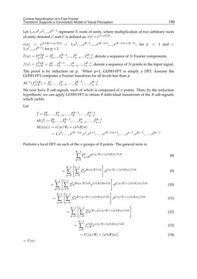
Cortical Specification of a Fast Fourier Transform Supports a Convolution Model of Visual Perception 19
Let 1, e, e2, e3, ..., eN−1 represent N roots of unity, where multiplication of two arbitrary rootsof unity denoted ei and ej is defined as: eiej = e(i+j)%N .
e(u) = e(u%B)+(u/B)n = 1, e1, ..., eB−1, ..., e(B−1)n, ..., e(B−1)n+(B−1), for p > 1 and =1, e1, ..., eB−1, for p = 1.
F(u) = Fu%Bu/B = F0
0 , ..., FB−10 , ..., F0
n−1, ...FB−1n−1 , denote a sequance of N Fourier components.
f (x) = f x%Bx/B = f 0
0 , ... f B−10 , ..., f 0
n−1, ..., f B−1n−1 , denote a sequence of N points in the input signal.
The proof is by induction on p. When p=1, GOSH-FFT is simply a DFT. Assume theGOSH-FFT computes a Fourier transform for all levels less than p.
M−1( f x%Bx/B ) = f 0
0 , . . . , f 0n−1, . . . , f B−1
0 , . . . , f B−1n−1 .
We now have B sub-signals, each of which is composed of n points. Then, by the inductionhypothesis, we can apply GOSH-FFT to obtain B individual transforms of the B sub-signals;which yields:
Let
f = F00 , . . . , F0
n−1, . . . , FB−10 , . . . , FB−1
n−1 .
M( f ) = F00 , . . . , FB−1
0 , . . . , F0n−1, . . . , FB−1
n−1
M(e(u)) = e((u/B) + (u%B)n)
= 1, en, . . . , e(B−1)n, e1, en+1, . . . , e(B−1)n+1, . . . , en−1, e2n−1, . . . , eBn−1
Perform a local DFT on each of the n groups of B points. The general term is:
B−1
∑q=0
Fqu/Beq((u/B)+((u%B)n))%N (8)
=B−1
∑q=0
[n−1
∑r=0
f qr eBr(u/B)%N
]eq(u/B)+((u%B)n))%N (9)
=B−1
∑q=0
[n−1
∑r=0
f qr eBn(u/B)%Ne(u%B)rBn%N
]eq((u/B)+((u%B))n))%N (10)
=B−1
∑q=0
[n−1
∑r=0
f qr eBr((u/B)+((u%B)n))%N
]eq((u/B)+((u%B)n))%N (11)
=B−1
∑q=0
[n−1
∑r=0
f qr e(Br+q)((u/B)+((u%B)n))%N
](12)
=N−1
∑s=0
f s%Bs/B es((u/B+((u%B)n))%N (13)
= F((u/B) + (u%B)n)) (14)
= F(u)
199Cortical Specification of a Fast FourierTransform Supports a Convolution Model of Visual Perception
20 Will-be-set-by-IN-TECH
Although this proof is for signals of size 7n represented on a hexagonal lattice, it applies to thecase of a signal of size 5n on a rectangular lattice with a few modifications, i.e. all appearancesof the number 7 needs to be replaced with the number 5.
8. Acknowlegements
The author thanks Valerie Christian McDougall for her work on improving the presentationof this manuscript.
The source code that implements GOSH-FFT is available in a software package namedVisioLab from the following website: http://www.ict.griffith.edu.au/sheridan/
9. References
Albright, T. D. & Desimone, R. (1987). Local precision of visuotopic organization in the middletemporal area (Mt) of the macaque. Experimental Brain Research, Vol. 65, No. 3, 1987,582-592
Alexander, D. M. & Bourke, P. D. (2004). Intrinsic connections in tree shrew V1 imply a globalto local mapping. Vision Research, Vol. 44, No. 9, 2004, 857-876
Alexander, D. M. & Wright, J. J. (2006). The maximum range and timing of excitatorycontextual modulation in monkey primary visual cortex. Visual Neuroscience, Vol. 23,No. 5, 2006, 721-728
Angelucci, A. & Levitt, J. B. (2002). Circuits for local and global signal integration in primaryvisual cortex. Journal of Neuroscience, Vol. 22, No. 19, 2002, 8633-8646
Bair, W. & Movshon, J. A. (2004) Adaptive temporal integration of motion indirection-selective neurons in macaque visual cortex. J Neurosci., Vol. 24, No. 33, 2004,7305-7323
Bartfeld, E. & A. Grinvald (1992). Relationships between Orientation-Preference Pinwheels,Cytochrome-Oxidase Blobs, and Ocular-Dominance Columns in Primate StriateCortex. Proceedings of the National Academy of Sciences of the United States of America,vol. 89, No. 24, pp. 11905-11909, 1992
Basole, A. & Kreft-Kerekes, V. (2006). Cortical cartography revisited: a frequency perspectiveon the functional architecture of visual cortex. Visual Perception, Part 1, Fundamentalsof Vision: Low and Mid-Level Processes in Perception Vol. 154, 2006, 121-134
Basole, A. & E. White, L. (2003). Mapping multiple features in the population response ofvisual cortex. Nature Vol. 23, No. 6943, 2003, 986-990
Berry, M. J. & Brivanlou, I. H. (1999). Anticipation of moving stimuli by the retina. Nature, Vol.398, No. 6725, 1999, 334-338
Blakemore, C. & Tobin, E. A. (1972). Lateral inhibition between orientation detectors in catsvisual-cortex. Exp Brain Res., Vol. 15, No. 4), 1972, 439-441
Blasdel, G. G. & Lund, J. S. (1985). Intrinsic Connections of Macaque Striate Cortex - AxonalProjections of Cells Outside Lamina 4C. Journal of Neuroscience, Vol. 5, No. 12, 1985,3350-3369
Blasdel, G. G. (1992). Orientation selectivity, preference, and continuity in monkey striatecortex. Journal of Neuroscience, Vol. 12, No. 8, 1992, 3139-61
Bosking, W. H. & Zhang, Y. (1997). Orientation selectivity and the arrangement of horizontalconnections in tree shrew striate cortex. Journal of Neuroscience, Vol. 17, No. 6, 1997,2112-2127
200 Fourier Transform Applications
Cortical Specification of a Fast Fourier Transform Supports a Convolution Model of Visual Perception 21
Briggs, F. & Usrey, W. M. (2007). A fast, reciprocal pathway between the lateral geniculatenucleus and visual cortex in the macaque monkey. Journal of Neuroscience, Vol. 27,No. 20, 2007, 5431-5436s
Bringuier, V. & Chavane, F. (1999). Horizontal propagation of visual activity in the synapticintegration field of area 17 neurons. Science, Vol. 283, No. 5402, 1999, 695-699
Bruce, V.; Green, P.R.; Georgeson, M. A. (2003). Visual perception physiology,psychology, andecology fourth edition, Psychology Press Taylor and Francis Group
Bullier, J. (2001). Feedback connections and conscious vision. Trends in Cognitive Sciences, Vol.5, No. 9, 2001, 369-370
Cavanaugh, J. R.; Bair, W.; Movshon, J. (2002) A. Selectivity and spatial distribution of signalsfrom the receptive field surround in macaque V1 neurons. J Neurophysiol., Vol. 88, No.5, 2002, 2547-2556
De Valois, K. K. & De Valois, R. L. (1979) Responses of Striate Cortex Cells to Grating andCheckerboard Patterns. Journal of Physiology-London, Vol. 291, Jun 1979, 483-505
Douglas, R. J. & Martin, K. A. C. (1991). A Functional Microcircuit for Cat Visual-Cortex.Journal of Physiology-London, Vol. 440, 1991, 735-769
Dudkin, K. (1992). Cooperative neural networks underlying image description in visualcortex. NeuROInformatics and Neurocomputers, Vol. 1, 1992, 387 - 398
Edwards, D. P. & Purpura, K. P. (1995). Contrast Sensitivity and Spatial-Frequency Responseof Primate Cortical-Neurons in and around the Cytochrome-Oxidase Blobs. VisionResearch, Vol. 35, No. 11, 1995, 1501-1523
Fiorani, M. & Rosa, M. G. (1992). Dynamic surrounds of receptive fields in primate striatecortex: a physiological basis for perceptual completion? Proceedings of the NationalAcademy of Sciences U S A, Vol. 89, No. 18, 1992, 8547-51
Fitzpatrick, D. & Lund, J. S. (1985). Intrinsic Connections of Macaque Striate Cortex - Afferentand Efferent Connections of Lamina 4C. Journal of Neuroscience, Vol. 5, No. 12, 1985,3329-3349
Foster, K. H. & Gaska, J. P. (1985). Spatial and temporal frequency selectivity of neurones invisual cortical areas V1 and V2 of the macaque monkey. Journal of Physiology, Vol. 365,1985, 331-63
Gao, Z. & Hu, B. (2001). Stochastic resonance of Small World Networks. Physicas Review, Vol.65, No. 16209, 1-4
Girard, P. & Hupe, J. M. (2001). Feedforward and feedback connections between areas V1 andV2 of the monkey have similar rapid conduction velocities. Journal of Neurophysiology,Vol. 85, No. 3, 2001, 1328-1331
Grigorescu, C.; Petkov N.; Westenberg, M. A. (2003) Contour detection based on nonclassicalreceptive field inhibition. IEEE Trans. Image Process., Vol. 12, No. 7, 2003, 729-739
Horton, J. C. & Hocking, D. R. (1998). Effect of early monocular enucleation upon oculardominance columns and cytochrome oxidase activity in monkey and human visualcortex. Visual Neuroscience, Vol. 15, No. 2, 1998, 289-303
Huang, W.; Jia, J.; Jia, J. ((2008) Modeling contextual modulation in the primary visual cortex.Neural Networks, Vol. 21, No. 8, 2008, 1182-1196
Huang, W.; Jiao, L.; Jia, J.; Yu, H. (2009) A neural contextual model for detecting perceptuallysalient contours. Pattern Recognition Letters, Vol. 30, No. 11, 2009, 985-993
Hubel, D. H. & Wiesel, T. N. (1962). Receptive Fields, Binocular Interaction and FunctionalArchitecture in Cats Visual Cortex. Journal of Physiology-London, Vol. 160, No. 1, 1962,106
201Cortical Specification of a Fast FourierTransform Supports a Convolution Model of Visual Perception

22 Will-be-set-by-IN-TECH
Hubel, D. H. & Wiesel, T. N. (1974). Sequence Regularity and Geometry of OrientationColumns in Monkey Striate Cortex. Journal of Comparative Neurology, Vol. 158, No.3, 1974, 267-294
Khayat, P. S. & Spekreijse, H. (2004). Correlates of transsaccadic integration in the primaryvisual cortex of the monkey. Proceedings of the National Academy of Sciences of the UnitedStates of America, Vol. 101, No. 34, 2004, 12712-12717
Kimura, R. & Ohzawa, I. (2009) Time course of cross-orientation suppression in the earlyvisual cortex. J Neurophysiol., Vol. 101, No. 3, 2009, 1463-1479
Kinoshita, M. & Komatsu, H. (2001). Neural representation of the luminance and brightnessof a uniform surface in the macaque primary visual cortex. Journal of Neurophysiology,Vol. 86, No. 5, 2001, 2559-2570
Kruger, J. & Fischer, B. (1975). Shift-Effect in Retinal Ganglion-Cells of Rhesus-Monkey.Experimental Brain Research, Vol. 23, No. 4, 1975, 443-446
Lamme, v. A. F. (1995). The neurophysiology of figure-ground segmentation in primary visualcortex. J. Neuroscience, Vol. 15, 1995, 1605-1615
Lamme, V. A. F.; Zipser, K.; Spekreijse, H. (1998). Figure-ground activity in primary visualcortex is suppressed by anesthesia. Proc Natl Acad Sci USA., Vol. 95, No. 6, 1998,3263-3268
Lee, T. S.; Mumford, D.; Romero, R.; Lamme, V. A. F. (1998). The role of the primary visualcortex in higher level vision. Vision Res., Vol. 38, No. 15, 1998, 2429-2454
Lee, H. C. & Choe, Y. (2003). Detecting salient contours using orientation energy distribution.Proc.Internat. Joint. Conf. on Neural Networks, Vol. 1, pp. 206-211
Leventhal, A. G. & Thompson, K. G. (1995). Concomitant Sensitivity to Orientation, Direction,and Color of Cells in Layer-2, Layer-3, and Layer-4 of Monkey Striate Cortex. Journalof Neuroscience, Vol. 15, No. 3, 1995, 1808-1818
Lund, J. S. & Angelucci, A. (2003). Anatomical substrates for functional columns in macaquemonkey primary visual cortex. Cerebral Cortex, Vol. 13, No. 1, 2003, 15-24
MacLennan, B. J. (1999). Field computation in natural and artificial intelligence. InformationSciences International Journal, Vol. 119 1999, 73-79
Malach, R. & Amir, Y. (1993). Relationship between Intrinsic Connections and FunctionalArchitecture Revealed by Optical Imaging and in-Vivo Targeted Biocytin Injectionsin Primate Striate Cortex. Proceedings of the National Academy of Sciences of the UnitedStates of America, Vol. 90, No. 22, 1993, 10469-10473
Marr, H. & Hildreth, E. (1980). Theory of edge detection. Proceedings of the Royal Society, Vol.B-207, 1980, 187-217
Marrocco, R. T. & McClurkin, J. W. (1982). Modulation of Lateral Geniculate-Nucleus CellResponsiveness by Visual Activation of the Cortico Geniculate Pathway. Journal ofNeuroscience, Vol. 2, No. 2, 1982, 256-263
Mikami, A. & Newsome, W. T. (1986). Motion selectivity in macaque visual cortex.II. Spatiotemporal range of directional interactions in MT and V1. Journal ofNeurophysiology, Vol. 55, No. 6, 1986, 1328-39
Murphy, K. M. & Jones, D. G. (1998). Spacing of cytochrome oxidase blobs in visual cortex ofnormal and strabismic monkeys. Cerebral Cortex, Vol. 8, No. 3, 1998, 237-244
Obermayer, K. & Blasdel, B. G. (1993). Geometry of Orientation and Ocular DominanceColumns in Monkey Striate Cortex. Journal of Neuroscience, Vol. 13, No. 10, 1993,4114-4129
202 Fourier Transform Applications

Cortical Specification of a Fast Fourier Transform Supports a Convolution Model of Visual Perception 23
Parker, A. J. & Hawken, M. J. (1988). Two-Dimensional Spatial Structure of Receptive-Fields inMonkey Striate Cortex. Journal of the Optical Society of America a-Optics Image Scienceand Vision, Vol. 5, No. 4, 1988, 598-605
Peters, A. & Sethares, C. (1996). Myelinated axons and the pyramidal cell modules in monkeyprimary visual cortex. Journal of Comparative Neurology, Vol. 365, No. 2, 1996, 232-255
Rockland, K. S. & Knutson, T. (2001). Axon collaterals of Meynert cells diverge over largeportions of area V1 in the macaque monkey. Journal of Comparative Neurology, Vol.441, No. 2, 2001, 134-147
Rockland, K. S. & Lund, J. S. (1983). Intrinsic Laminar Lattice Connections in PrimateVisual-Cortex. Journal of Comparative Neurology, Vol. 216, No. 3, 1983, 303-318
Rockland, K. S. & Saleem, K. S. (1994). Divergent Feedback Connections from Areas V4 andTeo in the Macaque. Visual Neuroscience, Vol. 11, No. 3, 1994, 579-600
Rockland, K. S. & Vanhoesen, G. W. (1994). Direct Temporal-Occipital Feedback Connectionsto Striate Cortex (V1) in the Macaque Monkey. Cerebral Cortex, Vol. 4, No. 3, 1994,300-313
Roelfsema, P. R. & Lamme, V. A. F. (1998). Object-based attention in the primary visual cortexof the macaque monkey. Nature, Vol. 395, No. 6700 376-381
Rolls, E. T. & Cowey, A. (1970). Topography of the retina and striate cortex and its relationshipto visual acuity in rhesus monkeys and squirrel monkeys. Experimental Brain Research,Vol. 10, No. 3, 1970, 298-310
Rossi, A. F. & Desimone, R. (2001). Contextual modulation in primary visual cortex ofmacaques. Journal of Neuroscience, Vol. 21, No. 5, 2001, 1698-1709
Sanger, T. D. (1988). Stereo disparity computation using Gabor filters. Biological Cybernetics,Vol. 59, 1988, 405-418
Sceniak, M. P.; Hawken, M. J.; Shapley, R. (2001). Visual spatial characterization of macaqueV1 neurons. J Neurophysiol., Vol. 85, No. 5, 2001, 1873-1887
Schiller, P. H. & Finlay, B. L. (1976). Quantitative Studies of Single-Cell Properties inMonkey Striate Cortex .2. Orientation Specificity and Ocular Dominance. Journal ofNeurophysiology, Vol. 39, No. 6, 1976, 1320-1333
Schiller, P. H. & Finlay, B. L. (1976). Quantitative studies of single-cell properties in monkeystriate cortex. III. Spatial frequency. J Neurophysiol, Vol. 39, No. 6, 1976, 1334-51
Sheridan, P.; Hintz, T.; Alexander, D. (2000). Pseudo invariant transformations on a hexagonallattice. Image Vision Comput., Vol. 18, No. 11, 2000, 907-917
Sheridan, P. E. (2007). A Method to Perform a Fast Fourier Transform with Primitive ImageTransformations. IEEE Transactions on Image Processing, Vol. 16, No. 5, 2007, 1355-1369
Siegel, R. M. (1990). Nonlinear dynamic system-theory primary visual cortical processing.Physica, Vol. 42, No. 1-3, 1990, 385-395
Sillito, A. M. & Jones, H. E. (1996). Context-dependent interactions and visual processing inV1. J Physiol Paris., Vol. 90, NO. 3-4, 1996, 205-209
Sirovitch, L.; Everson, R.; Kaplan, E.; Knight, B.; O’Brien, E.; Orbach, D. (1996). Modelling thefunctional organisation of the visual cortex. Physica, Vol. D96, 1996, 355-366
Stettler, D. D. & Das, A. (2002). Lateral connectivity and contextual interactions in macaqueprimary visual cortex. Neuron, Vol. 36, No. 4, 2002, 739-750
Tang, Q., Sang, N. & Zheng, P. (2007). Extraction of salient contours from cluttered scenes.Pattern Reccognition, Vol. 40, No. 11, 2007, 3100-3109
Tootell, R. B. H. & Hamilton, S. L. (1988). Functional-Anatomy of Macaque Striate Cortex.Journal of Neuroscience, Vol. 8, No. 5, 1988, 1500-1530
203Cortical Specification of a Fast FourierTransform Supports a Convolution Model of Visual Perception

24 Will-be-set-by-IN-TECH
Ursine, M.; La, G. E.; Cara (2004). A model of contextual interactions and contour detection inprimary visual cortex. Neural Networks, Vol. 17, No. 5-6, 2004, 719-735
Van Loan, C. (1992). Computational Frameworks for the Fast Fourier Transform, SIAM,Philadelphia, PA.
Wachtler, T. &. Sejnowski, T. J. (2003). Representation of color stimuli in awake macaqueprimary visual cortex. Neuron, Vol. 37, No. 4, 2003, 681-691
Zeki, S. (1993). A Vision of the Brain, Blackwell Scientific Publishing, Oxford.Zipser, K.; Lamme, V.; Schiller, P. (1996). Contextual modulation in primary visual cortex. J. of
Neuroscience, Vol. 16, No. 22, 1996, 736-738
204 Fourier Transform Applications

8
Spectral Analysis of Global Behaviour of C. Elegans Chromosomes
Afef Elloumi Oueslati1, Imen Messaoudi1, Zied Lachiri2 and Noureddine Ellouze1
Unité Signal, Image et Reconnaissance de Formes, Département de Génie Electrique, 1Ecole Nationale d’Ingénieurs de Tunis, BP 37, Campus Universitaire,
Le Belvédère, 1002, Tunis, 2Département de Génie Physique et Instrumentation
Institut National des Sciences Appliquées et de Technologie, BP 676, Centre Urbain Cedex, 1080, Tunis,
Tunisie
1. Introduction Fourier analysis is one of the most useful decomposition into frequency bands to provide a signal’s variations and irregularities measure. DNA spectral analysis based on Fourier Transform contributes in the systematic search of special DNA patterns which may correspond to biological important markers. For example, the Fourier harmonic analysis of the occurrence of a base “A” can give us the corresponding frequency with amplitude and a phase without being able to locate it in time. However it is interesting to also detect the moments of “silence” of base “A” i.e. the moments when this base does not exist. Such a representation of Fourier is thus limited with signals which contain transitory elements or evolutions in their spectral contents. For these non stationary signals, the DNA sequences, to highlight the frequency behavior, it becomes necessary to give the frequency the possibility of changes over time. It’s the time frequency analysis aim assured by the Short Time Fourier Transform. In fact, the punctual aspect is very important to localize particular regions in chromosomes, to characterize the beginning of a protein coding regions or a nucleosome or its end. By depicting the frequencies by a smoothed STFT, a 2D or 3D spectrogram representation, specific regions appear distinctly. In this paper, we are concerned with the periodicities 3, 6, 9 and 10.5. The periodicity 3 discussed in (Anastassiou, 2001; Berger et al, 2003; Cohanim et al, 2005; Kornberg, 1977; Segal et al, 2006; Susillo et al 2003; Trifonov & Sussman, 1980; Trifonov, 1998; Vaidyanathan & Yoon, 2004) is related with protein coding regions (called exons) in the gene. The periodicity 10.5 is related with nucleosome’s positions in the DNA sequence and the degree of deformability of the sequence in the DNA helix (Hayes et al, 1990; Trifonov & Sussman, 1980; Widom, 1996; Worcel et al 1981). The periodicity 6 and 9 are specific to C. Elegans organism.
This chapter is divided in five parts. First, we expose an introduction for relevant regions on chromosomes. In part three, we detailed the DNA’s sequence analysis approach, related to sequence global behavior problem. It exposes the spectral analysis, which follows a certain

Fourier Transform Applications
206
methodology that generates results to highlight the periodicities studied. This analysis is based on organisms translated into signals by three coding techniques. The algorithm steps of this technique are detailed to mention the generation method of spectrums and spectrograms. The fourth part deals with the study of the frequencies’ evolution. It present results for smoothed STFT, as a 1D, 2D or 3D spectrogram representation. Part five concludes this chapter.
2. The relevant regions in chromosomes The specific succession in the bases (A, G, C, and T) constitutes the hereditary message. Each DNA fragment involves a specific protein synthesis process. Proteins are synthesized from a set composed of 20 different amino acids, which are determined by three bases occurring in subsequent order. A group of three consecutive nucleotides with desoxyribose and phosphoric group is called a codon and a total of 64 different combinations specify 20 amino acids and three stop codons, namely TAA, TAG, and TGA. The protein synthesis (Fig.1) is realized in two steps: (1) the transcription within which the hereditary information is copied into the messenger RNA and, (2) the translation in which the messenger RNA is exploited by the ribosome to form the amino acid chain. To obtain numerical data from this succession of symbolic bases of a DNA sequence, we use binary indicator coding techniques.
genes
DNAsequence
Transcription
exon intronSplicing mRNA Traduction
Peptides
Fig. 1. The protein’s synthesis steps
In a DNA sequence, electron microscopy and biochemical studies have established that the bulk of the chromatin DNA is compacting into repeating structural units, named nucleosomes. A model of this DNA structure in such regions is proposed by Kornberg in (Kornberg, 1974, 1977). The chromatin is a dynamic structure, oscillating between the nucleosome and open structures depending on the environmental conditions (Kornberg, 1974, 1977; Oudet et al, 1978). And each nucleosome is formed by two molecules of each histone (protein) H2A,
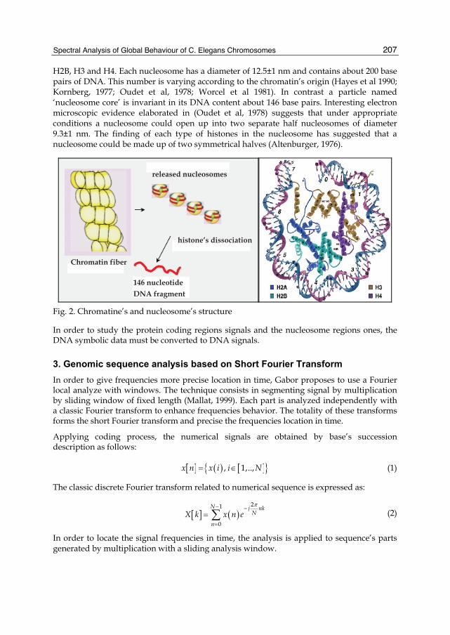
Spectral Analysis of Global Behaviour of C. Elegans Chromosomes
207
H2B, H3 and H4. Each nucleosome has a diameter of 12.5±1 nm and contains about 200 base pairs of DNA. This number is varying according to the chromatin’s origin (Hayes et al 1990; Kornberg, 1977; Oudet et al, 1978; Worcel et al 1981). In contrast a particle named ‘nucleosome core’ is invariant in its DNA content about 146 base pairs. Interesting electron microscopic evidence elaborated in (Oudet et al, 1978) suggests that under appropriate conditions a nucleosome could open up into two separate half nucleosomes of diameter 9.3±1 nm. The finding of each type of histones in the nucleosome has suggested that a nucleosome could be made up of two symmetrical halves (Altenburger, 1976).
released nucleosomes
histone’s dissociation
146 nucleotideDNA fragment
Chromatin fiber
Fig. 2. Chromatine’s and nucleosome’s structure
In order to study the protein coding regions signals and the nucleosome regions ones, the DNA symbolic data must be converted to DNA signals.
3. Genomic sequence analysis based on Short Fourier Transform In order to give frequencies more precise location in time, Gabor proposes to use a Fourier local analyze with windows. The technique consists in segmenting signal by multiplication by sliding window of fixed length (Mallat, 1999). Each part is analyzed independently with a classic Fourier transform to enhance frequencies behavior. The totality of these transforms forms the short Fourier transform and precise the frequencies location in time.
Applying coding process, the numerical signals are obtained by base’s succession description as follows:
[ ] ( ) [ ]{ }, 1,..,x n x i i N= ∈ (1)
The classic discrete Fourier transform related to numerical sequence is expressed as:
[ ] ( )21
0
N j nkN
nX k x n e
π− −
== ∑ (2)
In order to locate the signal frequencies in time, the analysis is applied to sequence’s parts generated by multiplication with a sliding analysis window.
Fourier Transform Applications
208
For this purpose, the numerical signal x[n] is divided into frames of N length. The expression become
[ ] [ ] [ ], .wx n i x n i nω Δ= − (3)
When based on the binary indicator ‘A’, the equation becomes:
[ ] [ ] [ ], .Aw Ax n i U n i nω Δ= − (4)
With i is the window’s order and the Δn is the adopted sliding value. The window’s length must be chosen to have an appropriate number of samples to guarantee the best frequency resolution. On each block xw [n], is applied a Fourier transform to determine Xw [k], k∈[0:N-1], k represents the frequency index. The FT expression associated with each frame is as follows:
[ ] [ ]21
0,
N j nki N
nX k x n i e
π
ω ω
− −
== ∑ (5)
With binary indicator ‘A’ coding, the equation is:
[ ] [ ]21
0,
N j nkN
A An
X k x n i eπ
ω
− −
== ∑ (6)
On the basis of this expression, many representations can be obtained. The sequence is associated to chromosome, the first analyze consists in studying the frequency global behavior. To enhance the frequencies, we used a mean smoothed spectrum. The principle consists in calculating the mean of the obtained spectrum of equation.
[ ] [ ]1
0
1 Nj i
iX k X k
Nω ω
−
== ∑ (7)
The chromosomes are generally constituted by more than 10 Mbp, so the obtained spectrum needs to be smoothed. A second mean of the mean spectrums is applied. The converted DNA sequence x[n] is divided into frames of M length with an overlap Δm. Each of these frames is also divided into N frames by multiplication with a sliding analysis window w[n]. On each part, a mean smoothed spectrum is generated. Finally, the mean of the spectrum for all the parts is calculated. The final expression of the spectrum is:
[ ] [ ]1
0
1 Mj
jX k X k
M ω
−
== ∑ (8)
3.1 The chromosomes coding techniques
This analysis aims to study the chromosome’s frequency global behaviour. For this purpose, it is important to enhance particularly the signals generated by the protein coding regions and the nucleosome regions. That’s why, three types of coding techniques are considered:

Spectral Analysis of Global Behaviour of C. Elegans Chromosomes
209
- A linear coding based on Binary indicators which is related to the base succession, - A Structural coding with Pnuc, which is an experimental coding based on the helix
deformability - A two-dimensional coding based on Frequency Chaos Game Representation which has
submerged from the field of physics known as 'chaotic dynamical systems'
3.1.1 Binary indicator’s techniques
The linear coding consists in attributing a binary value for each unit of the all indicators. Which are included in {’A’,’T’,’C’,’G’, ’TT’, ’TA’, ’GC’', ‘AAA’… ‘GGG’}. The marker associated takes the value of either 1 or 0 at location n for the first character, depending on whether or not the corresponding character group exists from the location n.
Base’s binary indicator:
[ ] [ ]bb B
S n U n∈
= ∑ (9)
Where:
[ ]1
0bif base b is in position n
U nelse
⎧= ⎨⎩
(10)
is the binary indicator of the base B={A,T,C,G}
Considering sequence DNAS and [ ]AU n the associated base’s binary indicator DNAS = ’AATCGCGACACTCATTCGG’ [ ]AU n = 1 1 0 0 0 0 0 1 0 1 0 0 0 1 0 0 0 0 0
Two Base’s binary indicator:
[ ] [ ]bbbb BB
S n U n∈
= ∑ (11)
where
[ ]1
0bbif base bb is in position n
U nelse
⎧= ⎨⎩
(12)
is the binary indicator of the base B
B={AA,AT,AC,AG,TA,TT,TC,TG,CA,CT,CC,CG,GA,GT,GC,GG}
Considering sequence DNAS and [ ]CGU n the associated base’s binary indicator DNAS = ’AATCGCGACACTCATTCGG’
[ ]CGU n = 0 0 0 1 0 1 0 0 0 0 0 0 0 0 0 0 1 0
Some dinucleotides as ‘AA’, ’TT’, ‘TA’ are enhancing the ADN flexibility around histones to constitute nucleosomes (Fig. 3).
Codon’s binary indicator: the three bases association called triplet or codon have a fundamental role in the process of amino acids fabrication. For these reasons, a coding

Fourier Transform Applications
210
technique based on these base’s association is used. We adopt binary indicators to each of the 64 codons (Table 1)
[ ] [ ]{ }, 1cod sS n U i i N= = … (13)
where:
[ ]1
0codif the codon cod starts at position n
U ielse
⎧= ⎨⎩
(14)
is the binary indicator of the codon cod and Ns is the sequence’s length. This marker takes the value of either 1 or 0 at location n for the first character depending on whether the corresponding character exists from the location n. Let’s consider the codon binary indicator
[ ]TCGU n .
Considering sequence DNAS and the associated codon’s binary indicator DNAS = ’AATCGCGACACTCATTCGG’
[ ]TCGU n = 0 0 1 0 0 0 0 0 0 0 0 0 0 0 1 0
Fig. 3. DNA flexibility around histones is enhanced by dinucleotide as ‘AA’, ’TT’, ‘TA’
BASE Codon associated
A AAA, AAT, AAC, AAG, ATA, ATT, ATC, ATG ACA, ACT, ACC, ACG, AGA, AGT, AGC, AGG
T TAA, TAT, TAC, TAG,TTA, TTT, TTC, TTG TCA, TCT, TCC, TCG, TGA, TGT, TGC, TGG
C CAA, CAT, CAC, CAG, CTA, CTT, CTC, CTG CGT, CGC, CGG, CCA, CCT, CCC, CCG, CGA
G GAA, GAT, GAC, GAG, GTA, GTT, GTC, GTG GCA, GCT, GCC, GCG, GGA, GGT, GGC, GGG
Table 1. Codon associated to each base

Spectral Analysis of Global Behaviour of C. Elegans Chromosomes
211
3.1.2 Pnuc: the structural coding techniques
The second coding technique is the Pnuc which is based on local bending and flexibility properties of the double helix; it is deduced experimentally from nucleosome positioning (Pnuc). By considering the matching of both stalks (A-T and C-G) along the helix, one base’s pair defines a plane and a direction in this plane. A description of the double helix shows the overlapping of the plans (Fig. 4). When considering that the planes are parallel, passing between planes needs translation and rotation of 34,3° of the orientation of the connection of the plan.
Fig. 4. A description of the double helix shows the overlapping of the plans
Now the plans are not parallel and the axis of the double helix presents curvature. By considering the interaction between a protein, a histone and a DNA’s sequence, this interaction is stronger when the contact area between both objects is the biggest. To increase this surface, it is necessary to roll up as much as possible the segment of DNA around the protein, in this way, we have two properties:
If the segment of DNA is not rolled up around the protein, it is in position of equilibrium, the curvature is static
The stalk must be flexible to allow the additional curvature around the protein. These two properties generate the nucleosome which generates an excessive curvature of the stalk.
Each trinucleotide is replaced by its numerical value given by the Pnuc table. The DNAS is then replaced by the numerical sequence PNUCC .
DNAS = ’AATCGCGACACTCATTCGG’ PNUCC = 0.7 5.3 8.3 7.5 7.5 6.0 5.4 5.2 6.5 5.8 5.4 5.4 6.7 0.7 3.0 8.3 4.7

Fourier Transform Applications
212
Trinucleotide PNUC Trinucleotide PNUC AAA/TTT 0.0 CAG/CTG 0.042 AAC/GTT 0.037 CCA/TGG 0.054 AAG/CTT 0.052 CCC/GGG 0.060 AAT/ATT 0.07 CCG/CGG 0.047 ACA/TGT 0.052 CGA/TCG 0.083 ACC/GGT 0.054 CGC/GCG 0.075 ACG/CGT 0.054 CTA/TAG 0.022 ACT/AGT 0.058 CTC/GAG 0.054 AGA/TCT 0.033 GAA/TTC 0.030 AGC/GCT 0.075 GAC/CTG 0.054 AGG/CCT 0.054 GCA/TGC 0.060 ATA/TAT 0.028 GCC/GGC 0.0100 ATC/GAT 0.053 GGA/TCC 0.038 ATG/CAT 0.067 GTA/TAC 0.037 CAA/TTG 0.033 TAA/TTA 0.020 CAC/GTG 0.065 TCA/TGA 0.054
Table 2. The PNuc table
The signal generated from this coding for a part of chromosome is given by Fig. 5. For clarity purpose the signal is multiplied by 10. Fig. 6 illustrate the stft method applied on this resulting signal. First, subfigure a shows a mean spectrum for distinct window of length 5*105.. The spectrum obtained needs smoothing so for the second figure (subfigure b) a blackman smoothing window is applied on each signal part before calculating the mean spectrum of equation 7. In the third and last figures (subfigure c and d) the equation 8 is used and the parameters chosen are: Blackman window, M=5*105 , N=5*104 and overlap 50% for subfigure c and N=5*103 with overlap 10% for subfigure d. The figure shows that meaning and smoothing are very efficient to have the best signal (subfigure d). In this signal, the periodicity 10 is enhanced to prove that this is a characteristic of helix flexibility.
Fig. 5. Pnuc signal of 2000 base pairs of chromosome 1 of C. Elegans genome

Spectral Analysis of Global Behaviour of C. Elegans Chromosomes
213
Fig. 6. Illustration of the smoothed mean spectrum applied on Pnuc signal of 2000 base pairs of chromosome 1 of C. Elegans genome
3.1.3 Fcgr: the two dimensionnal coding techniques
The third technique is submerged from the Chaos Game Representation (CGR) images which can forms a global signature of bio-sequences (Almeida et al, 2001; Cenac et al, 2004; Deshavanne et al, 1999, 2000; Joseph & Sasikumar, 2006; Oliver et al 1993; Fiser et al, 1994). The CGR paradigm is a holistic way of DNA representation. It provides a unique scatter pictures. In 1999, H. Joel Jeffrey uses for the first time this representation for studying the "non-randomness" of genomic sequences (Jeffrey, 1990). The CGR is an iterative algorithm for drawing fractal images to any desired scale. It maps nucleotide sequences in the [0,1]x[0,1] square. The four letters A, C, G and T are placed at the corners. The binary CGR vertices are assigned to the four nucleotides as:
( ) ( ) ( ) ( )0,0 , 0,1 , 1,1 , 1,0A C G Tl l l l= = = = (15)
Deriving scatter pictures, the CGR’s construction algorithm consists of three steps. First, the four letters A, C, G and T are placed at the corners of a rectangular unit square. Second, the first point is plotted halfway between the center of the square, and the corner corresponding
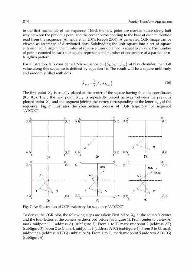
Fourier Transform Applications
214
to the first nucleotide of the sequence. Third, the new point are marked successively half way between the previous point and the corner corresponding to the base of each nucleotide read from the sequence (Almeida et al, 2001; Joseph 2006). A generated CGR image can be viewed as an image of distributed dots. Subdividing the unit square into a set of square entries of equal size n, the number of square entries obtained is equal to 2n ×2n. The number of points counted in each sub-square represents the number of occurrence of a particular n-lengthen pattern.
For illustration, let’s consider a DNA sequence { }1 2, ,...., NS S S S= of N nucleotides, the CGR value along this sequence is defined by equation 16. The result will be a square uniformly and randomly filled with dots.
( )1112 nn n sX X l
++ = + (16)
The first point 0X is usually placed at the center of the square having thus the coordinates (0.5, 0.5). Then, the next point 1nX + is repeatedly placed halfway between the previous plotted point nX and the segment joining the vertex corresponding to the letter 1ns + of the sequence. Fig. 7 illustrates the construction process of CGR trajectory for sequence "ATCGG".
Fig. 7. An illustration of CGR trajectory for sequence ″ATCGG″
To derive the CGR plot, the following steps are taken: First place 0X at the square’s center and the four letters at the corners as described before (subfigure 1). From center to vertex A, mark midpoint 1 ( address A) (subfigure 2). From 1 to T, mark midpoint 2 (address AT) (subfigure 3). From 2 to C, mark midpoint 3 (address ATC) (subfigure 4). From 3 to G, mark midpoint 4 (address ATCG) (subfigure 5). From 4 to G, mark midpoint 5 (address ATCGG) (subfigure 6).
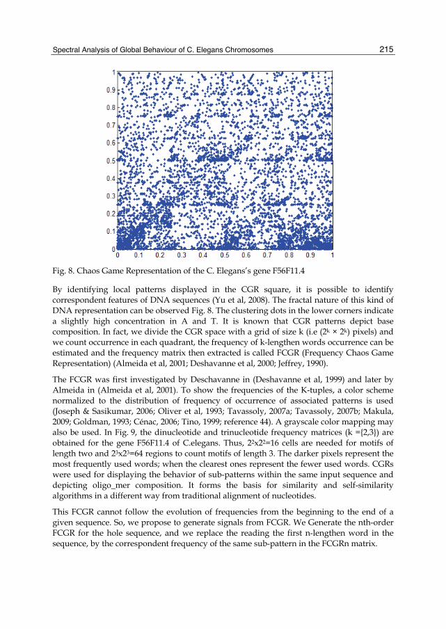
Spectral Analysis of Global Behaviour of C. Elegans Chromosomes
215
Fig. 8. Chaos Game Representation of the C. Elegans’s gene F56F11.4
By identifying local patterns displayed in the CGR square, it is possible to identify correspondent features of DNA sequences (Yu et al, 2008). The fractal nature of this kind of DNA representation can be observed Fig. 8. The clustering dots in the lower corners indicate a slightly high concentration in A and T. It is known that CGR patterns depict base composition. In fact, we divide the CGR space with a grid of size k (i.e (2k × 2k) pixels) and we count occurrence in each quadrant, the frequency of k-lengthen words occurrence can be estimated and the frequency matrix then extracted is called FCGR (Frequency Chaos Game Representation) (Almeida et al, 2001; Deshavanne et al, 2000; Jeffrey, 1990).
The FCGR was first investigated by Deschavanne in (Deshavanne et al, 1999) and later by Almeida in (Almeida et al, 2001). To show the frequencies of the K-tuples, a color scheme normalized to the distribution of frequency of occurrence of associated patterns is used (Joseph & Sasikumar, 2006; Oliver et al, 1993; Tavassoly, 2007a; Tavassoly, 2007b; Makula, 2009; Goldman, 1993; Cénac, 2006; Tino, 1999; reference 44). A grayscale color mapping may also be used. In Fig. 9, the dinucleotide and trinucleotide frequency matrices (k ={2,3}) are obtained for the gene F56F11.4 of C.elegans. Thus, 22x22=16 cells are needed for motifs of length two and 23x23=64 regions to count motifs of length 3. The darker pixels represent the most frequently used words; when the clearest ones represent the fewer used words. CGRs were used for displaying the behavior of sub-patterns within the same input sequence and depicting oligo_mer composition. It forms the basis for similarity and self-similarity algorithms in a different way from traditional alignment of nucleotides.
This FCGR cannot follow the evolution of frequencies from the beginning to the end of a given sequence. So, we propose to generate signals from FCGR. We Generate the nth-order FCGR for the hole sequence, and we replace the reading the first n-lengthen word in the sequence, by the correspondent frequency of the same sub-pattern in the FCGRn matrix.
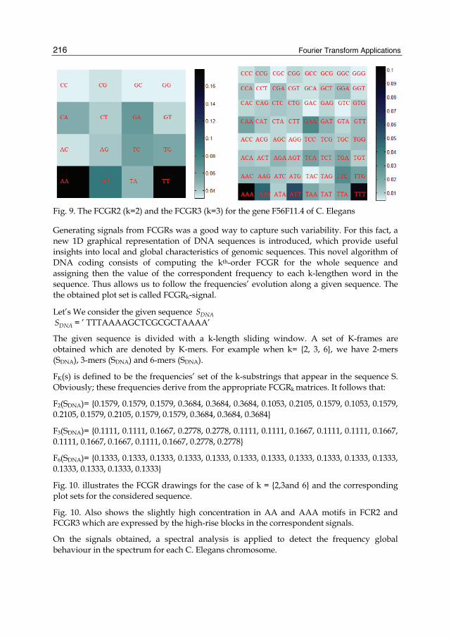
Fourier Transform Applications
216
Fig. 9. The FCGR2 (k=2) and the FCGR3 (k=3) for the gene F56F11.4 of C. Elegans
Generating signals from FCGRs was a good way to capture such variability. For this fact, a new 1D graphical representation of DNA sequences is introduced, which provide useful insights into local and global characteristics of genomic sequences. This novel algorithm of DNA coding consists of computing the kth-order FCGR for the whole sequence and assigning then the value of the correspondent frequency to each k-lengthen word in the sequence. Thus allows us to follow the frequencies’ evolution along a given sequence. The the obtained plot set is called FCGRk-signal.
Let’s We consider the given sequence DNAS DNAS = ’ TTTAAAAGCTCGCGCTAAAA’
The given sequence is divided with a k-length sliding window. A set of K-frames are obtained which are denoted by K-mers. For example when k= {2, 3, 6}, we have 2-mers (SDNA), 3-mers (SDNA) and 6-mers (SDNA).
FK(s) is defined to be the frequencies’ set of the k-substrings that appear in the sequence S. Obviously; these frequencies derive from the appropriate FCGRk matrices. It follows that:
F2(SDNA)= {0.1579, 0.1579, 0.1579, 0.3684, 0.3684, 0.3684, 0.1053, 0.2105, 0.1579, 0.1053, 0.1579, 0.2105, 0.1579, 0.2105, 0.1579, 0.1579, 0.3684, 0.3684, 0.3684}
F3(SDNA)= {0.1111, 0.1111, 0.1667, 0.2778, 0.2778, 0.1111, 0.1111, 0.1667, 0.1111, 0.1111, 0.1667, 0.1111, 0.1667, 0.1667, 0.1111, 0.1667, 0.2778, 0.2778}
F6(SDNA)= {0.1333, 0.1333, 0.1333, 0.1333, 0.1333, 0.1333, 0.1333, 0.1333, 0.1333, 0.1333, 0.1333, 0.1333, 0.1333, 0.1333, 0.1333}
Fig. 10. illustrates the FCGR drawings for the case of k = {2,3and 6} and the corresponding plot sets for the considered sequence.
Fig. 10. Also shows the slightly high concentration in AA and AAA motifs in FCR2 and FCGR3 which are expressed by the high-rise blocks in the correspondent signals.
On the signals obtained, a spectral analysis is applied to detect the frequency global behaviour in the spectrum for each C. Elegans chromosome.

Spectral Analysis of Global Behaviour of C. Elegans Chromosomes
217
(a) FCGR2 (b) FCGR2-signal
(c) FCGR3 (d) FCGR3-signal
(e) FCGR6 (f) FCGR6-signal
Fig. 10. FCG representation for k=2, 3 and 6 and the FCGR_signals associated

Fourier Transform Applications
218
3.2 The Fourier analysis method steps
The short time analysis is the technique used in order to locate specific regions in a DNA sequence. In this purpose, a mean values of Smoothed Discrete Fourier Transform is applied on sliding window along the DNA sequence to follow the peak’s evolution for specific frequencies points. The Fourier analysis algorithm steps are:
The converted DNA sequence x[n] is divided into frames of M length with an overlap Δm. Each of these frames is also divided into N frames by multiplication with a sliding analysis window w[n]:
[ , ] [ ] [ ]wx n i x n w n i nΔ= − (17)
Where i is the window index, and Δn the overlap. The weighting w[n] is assumed to be non zero in the interval [0, N-1]. The frame length value N is chosen in such a way that, on the one hand, the parameters to be measured remain constant and, on the other hand, that there are enough samples of x[n] within the frame to guarantee reliable frequency parameter determination. The choice of the windowing function influences the values of the short term parameters, the shorter the window the greater his influence (Mallat, 1999). We select N and M frame length as power of two to apply the Fast Fourier Transform algorithm.
Each weighted block xw[n], of the frame is transformed in the spectral domain using Discrete Fourier Transform (DFT), in order to extract the spectral parameters Xw[k], where k represents the index of the frequency ([0, N-1]). The DFT of each frame (in one of M sequence parts) is expressed as follows:
21
0[ ] [ , ]
N j nki Nw w
nX k x n i e
π− −
== ∑ (18)
Using the mean values, we calculate a DFT mean value for each frame (1: M). The expression of mean DFT is expressed as:
1
0
1[ ] [ ]N
j iw w
iXm k X k
N
−
== ∑ (19)
Where i correspond to the index frame of N frames ([1...N]), k is the index of the frequency and j correspond to the index frame of M frames ([1: M]). We constitute the matrix
( ), [ ]jwMAT j k Xm k= (20)
With these obtained values, we can constitute the matrix to represent restricted join time frequency information, known as 2D or 3D DNA spectrograms. This 2D or 3D representation consists of the spectrogram amplitude for a specific index periodicity in a specific nucleotide position in the chromosome.
4. Results The method has been applied on C. Elegans genome. The chromosomes have been divided on 1- million’s parts. The M frames have a length of 1024 bp and an overlap Δm=256, the

Spectral Analysis of Global Behaviour of C. Elegans Chromosomes
219
N frames of each M frames have length of 256 with Δn =128. The fig. 11 presents some examples for the spectrum related to each of the three coding technique used. In this figure, we show particularly the periodicities 3 and 10 which are closely depending on coding.
Fig. 11. Examples of spectrums and spectrograms generated with a mean valued technique based on smoothed Discrete Fourier Transform applied on sliding window along the DNA sequence parts of C. elegans genome. Two coding methods are used: a- linear coding technique (binary indicator) (subfigure a), b- structural coding technique (PNUC) (subfigure b)
In order to highlight the various frequencies characteristic of an organism, the tests were carried out with various coding over various sizes of segments and various widths. The example presented in the Table 3 presents the percentage of contribution of the trinucleotides in the highlighting of the various characteristic frequencies at the frequencies 1/3, 1/6.5, 1/9 and 1/10. The table shows that the organism C. Elegans is rich in periodicities and that these periodicities are raised by more than the 3/4 of these coding technique. We notice clearly that for periodicity 3, the rate has raised more 97 %, followed by periodicity 10 which has 90 % and periodicity 9 with 85 %. Periodicity 6.5 is a periodicity which is very marked for this organism 70 % of code contributes to its raising. It translates the existence with a very high rate of 6 bases groups at the periodicity 6. The majority of these groups represent polyA, generally associated for gene purposes.
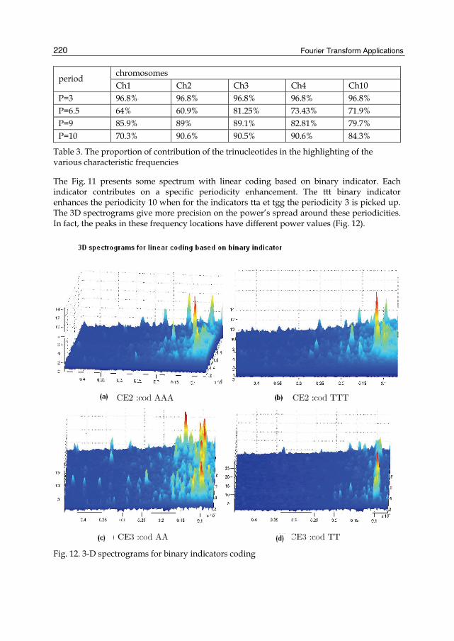
Fourier Transform Applications
220
chromosomes period Ch1 Ch2 Ch3 Ch4 Ch10
P=3 96.8% 96.8% 96.8% 96.8% 96.8% P=6.5 64% 60.9% 81.25% 73.43% 71.9% P=9 85.9% 89% 89.1% 82.81% 79.7% P=10 70.3% 90.6% 90.5% 90.6% 84.3%
Table 3. The proportion of contribution of the trinucleotides in the highlighting of the various characteristic frequencies
The Fig. 11 presents some spectrum with linear coding based on binary indicator. Each indicator contributes on a specific periodicity enhancement. The ttt binary indicator enhances the periodicity 10 when for the indicators tta et tgg the periodicity 3 is picked up. The 3D spectrograms give more precision on the power’s spread around these periodicities. In fact, the peaks in these frequency locations have different power values (Fig. 12).
Fig. 12. 3-D spectrograms for binary indicators coding

Spectral Analysis of Global Behaviour of C. Elegans Chromosomes
221
The spectrogram 3D adds a third element to the representation 2D. In addition to the localization of the periodicities in the segment, we visualize power associated with each peak. We can distinguish between the peaks which we can find in all the segments for a given periodicity: 10 and 3 and the peaks which are present in certain segments and which were eliminated by carrying out the average
The Fig. 12 is divided on 4 subfigures. Each one add to the 2D spectrograms the power values and locations of the periodicities Enhanced: it represents the 3-D spectrograms. Subfigures (a) and (b) are related to chromosomes2 of C. Elegans when the subfigures (c) and (d) concern chromosome 3.
This figure shows that for the binary indicator ‘AA’, ‘TT’, ‘AAA’ and ‘TTT’, the peaks around the frequency 1/10.5 are very pronounced. The variation of the degree view angle demonstrates that the peaks are locally spread in the chromosome part. In the literrature, it has been demonstrated both with the biochemical and signal processing studies, that the periodicity 10.5 related to the nucleosomes is varying. That’s why, these figures shows in one hand that there is peaks around this periodicity and in the other hand the peaks are spread in specific regions in the chromosome.
The Fig. 13 represents the spectrograms recovered after PNUC coding. The analysis breaks up the chromosome made up of 15,2Mbp into 15 parts of 1Mbp. We find the localization of the periodicity in the ends. In reality, the periodicity peaks are missed or have of very weak power in the sequence going of 6 Mbp with 12 Mbp, it is not localized on the centromer but it is around ends of the helix. We find it towards the position 13 Mbp until the end. In the parts where it exists it is not continuous, it is localized in specific time’s lapses.
In Fig. 14 mean valued technique based on smoothed Discrete Fourier Transform was applied along the parts 6, 9 and 13 of the chromosome 1 of C.elegans. From the 1D, 2D and 3D plots, it is observed that coding with FCGR2 reveal the presence of both 10.5 and 3 periodicities. The peaks are spread with different values according to parts around each of these periodicities. Each part has each own specificity. In fact, in part 9 (subfigure a) , periodicities 3 and 10 just submerge from the frequency behavior with peaks of modest values. For the part 6 these periodicities have the same behavior, the specificity is the presence of horizontal peaks around the location 750 in this part. When the part 13 is rich in periodicities 10 and 12 and poor in periodicity 3.
For coding with FCGR-3 (Fig.15), the very pronounced peaks correspond to the 10.5 periodicity; just in the left side other peaks appear around the frequency 0.11 which corresponds to the 9 periodicity; in the right side a few peaks occur around the frequency 1/12. The 3 periodicity disappears in the majority of the parts and when it appears, it is present only on a few areas with very low amplitudes. In Fig 15, we can distinguish between frequency behavior in the three parts represented. The periodicity 10 is more pronounced for the part 16 (subfigure b) when comparing with part 9 (subfigure a) and 10 (subfigure c).
As for the hexamers coding (FCGR6), we find that it enhances the frequency 1/10.5; upon rare zones the frequency 1/12 is observed (Fig.16). We clearly notice that this coding technique enhances the periodicity 10 and his neighbor in opposition to periodicity 3. The three parts shows different aspect of the repartition of the periodicities. In part 9 (subfigure a), the peaks are spread in a “large” frequency band around periodicity. The band is reduced for part 16 (subfigure b) to be located in two frequencies then the power is grouped in one frequency for part 12 (subfigure c).
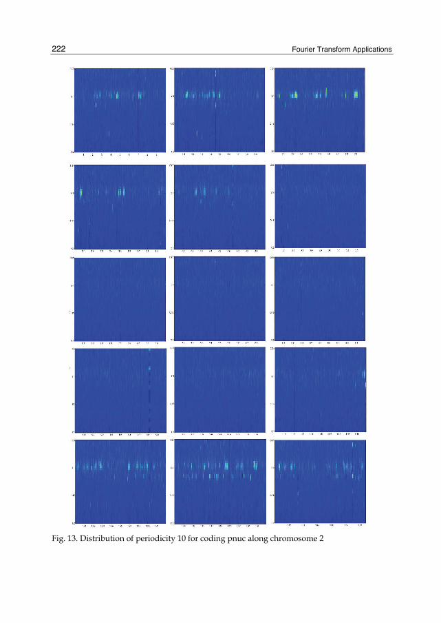
Fourier Transform Applications
222
Fig. 13. Distribution of periodicity 10 for coding pnuc along chromosome 2

Spectral Analysis of Global Behaviour of C. Elegans Chromosomes
223
0.05 0.1 0.15 0.2 0.25 0.3 0.35 0.4 0.45 0.510
20
30
40
50
500 1000 1500 2000 2500 3000 3500
0.1
0.2
0.3
0.4
a- Fourier analysis of part 9 of chromosome 1
0.05 0.1 0.15 0.2 0.25 0.3 0.35 0.4 0.45 0.510
20
30
40
50
500 1000 1500 2000 2500 3000 3500
0.1
0.2
0.3
0.4
b- Fourier analysis of part 6 of chromosome 1
0.05 0.1 0.15 0.2 0.25 0.3 0.35 0.4 0.45 0.510
20
30
40
50
60
500 1000 1500 2000 2500 3000 3500
0.1
0.2
0.3
0.4
c- Fourier analysis of part 13 of chromosome 1
Fig. 14. Examples of spectrums and spectrograms of chromosome’s parts with FCGR-2 signal coding
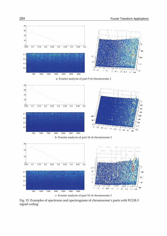
Fourier Transform Applications
224
0.05 0.1 0.15 0.2 0.25 0.3 0.35 0.4 0.45 0.55
10
15
20
25
500 1000 1500 2000 2500 3000 3500
0.1
0.2
0.3
0.4
a- Fourier analysis of part 9 of chromosome 1
0.05 0.1 0.15 0.2 0.25 0.3 0.35 0.4 0.45 0.55
10
15
20
25
500 1000 1500 2000 2500 3000 3500
0.1
0.2
0.3
0.4
b- Fourier analysis of part 16 of chromosome 1
0.05 0.1 0.15 0.2 0.25 0.3 0.35 0.4 0.45 0.55
10
15
20
500 1000 1500 2000 2500 3000 3500
0.1
0.2
0.3
0.4
c- Fourier analysis of part 10 of chromosome 1
Fig. 15. Examples of spectrums and spectrograms of chromosome’s parts with FCGR-3 signal coding

Spectral Analysis of Global Behaviour of C. Elegans Chromosomes
225
0.05 0.1 0.15 0.2 0.25 0.3 0.35 0.4 0.45 0.50.2
0.4
0.6
0.8
1
1.2
500 1000 1500 2000 2500 3000 3500
0.1
0.2
0.3
0.4
a- Fourier analysis of part 9 of chromosome 1
0.05 0.1 0.15 0.2 0.25 0.3 0.35 0.4 0.45 0.50
0.5
1
1.5
500 1000 1500 2000 2500 3000 3500
0.1
0.2
0.3
0.4
b- Fourier analysis of part 16 of chromosome 1
0.05 0.1 0.15 0.2 0.25 0.3 0.35 0.4 0.45 0.50
0.5
1
1.5
2
500 1000 1500 2000 2500 3000 3500
0.1
0.2
0.3
0.4
c- Fourier analysis of part 12 of chromosome 1
Fig. 16. Examples of spectrums and spectrograms of chromosome’s parts with FCGR-6 signal coding
Fourier Transform Applications
226
A peak around the frequency 1 / 4 nearby at position 2500 corresponds to a satellite (Fig. 16 subfigure a). This frequency derives from repetitions of certain dinucleotides in the area. The spectrogram reveals the presence of a satellite with multiple frequencies; this is manifested clearly in the 3D graph in the form of horizontally aligned peaks colored in red, the higher frequencies.
5. Conclusion In This chapter, we investigate the contribution of each coding technique: the linear, the two-dimensional and the structural one in the enhancement of the peaks related to the C. elegans genome periodicities. For this purpose, we use a mean values of smoothed Discrete Fourier Transform applied on sliding window along the DNA sequence to follow the peak evolution for specific frequency points around the frequencies. We detect periodicities around 3, 6, 9 and 10 and found periodicities 3 and 10 related respectively to genes and the positions of the nucleosomes. First we evaluate the frequencies spread through the chromosomes with a 1-D spectrum. Second, we consider the 2-D and 3-D DNA spectrograms to visually detect the specific parts of chromosomes related with protein coding regions, nucleosomes positioning regions, and other particular regions.
The time frequency analysis made it possible to follow the periodicities’ evolution. We studied the contribution of a range of binary indicators for the raising of exons’ peak frequency. We also studied the localization of the areas being able to form nucleosomes. Thanks to the spectrogram with two dimensions, we visualized the localization of the areas corresponding to periodicity 10 in the limits and not in the center of the helix. The three-dimensional spectrogram showed that the raised peaks do not correspond to the periodicity 10 but we see clearly in certain sequences and for some indicators two lines of peaks of variable powers around this periodicity. This result can explain the variation between 10 and 10.7 of the periodicities associated with the nucleosomes presented in the literature. It is also observable that these peaks are alternated around two periodicities; this result could be associated with the phenomena of chromatin compaction.
6. References Almeida, J.S., Carrico, J.A., Maretzek, A., Noble P.A. & Fletcher M. (2001) “Analysis of
genomic sequences by Chaos GameRepresentation”, Bioinformatics Vol. 17, n°5, pp 429–437.
Anastassiou D. (2001), “Genomic Signal processing”, IEEE Signal Processing Magazine, 18 (4), pp: 8-20.
Berger J. A., Mitra S. K.& Astola J. (2003), “Power spectrum analysis for DNA sequences”, Proc. of ISSPA 2003, pp 29-32, France, 1-4 July.
Cénac, P. (2006) “Étude statistique de séquences biologiques et convergence de martingales”, PhD thesis on Applied Mathematics, Paul Sabatier University, Toulouse III, pp 17−25.
Cénac P., Fayolle G., Lasgouttes J.M., (2004) “ Dynamical Systems in the Analysis of Biological Sequences”, research report n° 5351,pp 3–50.
Cohanim, A.B., Kashi Y. & Trifinov E.N. (2005), “Yeast Nucleosome DNA Pattern: Deconvolution from Genome Squences of S. cerevisiae, Journal of Biomolecular Structure & Dynamics ISSN 0739-1102, volume 22, Issue Number 6, Adenine Press, pp: 687-693.

Spectral Analysis of Global Behaviour of C. Elegans Chromosomes
227
Deschavanne, P., Giron, A., Vilain, J. Dufraigne, CH., & Fertil, B. (2000), “Genomic Signature Is Preserved in Short DNA Fragment”, International Symposium on Bio-Informatics and Biomedical Engineering, IEEE, pp 161–167.
Deschavanne, P., Giron, A., Vilain, J., Fagot, G. & Fertil, B. (1999) “Genomic signature: characterization and classification of species assessed by chaos game representation of sequences”, Mol Biol E, Vol 16, n°10, pp 1391–1399.
Fiser, A., Tusnady, G.E.& Simon, I.(1994) “Chaos game representation of protein structures”, J.Mol Graphics, Vol 12, pp 295,302–304.
Fukushima, A., Ikemurab, T., Kinouchie, M., Oshima, T., Kudod, Y., Morig, H. & Kanaya, S. (2002) “Periodicity in prokaryotic and eukaryotic genomes identified by powerspectrum analysis”, Elsevier, Gene 300, pp 203–211.
Goldman, N. (1993) “Nucleotide, dinucleotide and trinucleotide frequencies explain patterns observed in chaos game representations of DNA sequences”, Nucleic Acids Research Vol.21, n°10, pp 2487–2491.
Godsell, D.S. & Dickerson, R.E. (1994) “Bending and curvature calculations in b-dna”, Nucl. Acids Res, vol 22, pp 5497-5503.
Hayes, J.J., Tullius, T.D. & wolffe, A. P. (1990) “The structure of DNA in a nucleosome”, Proceedings of the National Academy of sciences of the United States of America, vol 87 No 19, pp 7405-7409, October.
Jeffrey, H.J., (1990) “Chaos game visualization of sequences”, Computers & Graphics, Elsevier, Vol.16, n°1, pp 25–33.
Joseph, J. & Sasikumar, R. (2006) “Chaos game representation for comparison of whole genomes”, BMC Bioinformatics, Vol 7, n°1, pp 1-10..
Kornberg, R.D. (1974), “Chromatin structure: a repeating unit of histones and DNA.” Science 184, pp:868-871,
Kornberg, R.D. (1977), “Structure of Chromatin”, Annu Rev Biochem. 46 , pp 931-954. Makula, M., (2009) “Interactive visualization of oligomer frequency in DNA” Computing and
Informatics, Vol. 28, pp 1001–1016. Nicorici, D., Berger, J. A. , Astola, J. & Mitra, S. K. ,(2003), “Finding borders between coding and
non coding DNA regions using recursive segmentation and statistics of stop codons”, Finnish Signal Processing Symposium (FINSIG'03), Tampere, Finland, pp. 231-235.
Oliver, J. L., Bernaola-Galvan, P., Guerrero, G. & Foman-Roldan, R. (1993), “Entropic profiles of DNA sequences through chaos-game-derived images,” J. Theor. Biol.,Vol 160, n°4, pp 457–470.
Oppenheim, A. V., Schafer ,R. W. & Buck, J. R., (1999) “Discrete Time Signal Processing”, 2nd Edition, Prentice Hall.
Oudet, P., Germond, J.E., Bellard, M., Spadafora, C. & Chambon, P. (1978) “Structure of Eucaryotic Chromosomes and Chromatin”, Phylosophical Transactions of the Royal Society of London. Series B, Biological Sciences, vol 283, No 997, pp: 241-258,
Segal, E., Fondufe-Mittendorf, Y., Chen, L., Thamstrom, A., Field, Y., Moore, I. K., Wang, J.P.Z. & widom, J. (2006) “ a genomic code for nucleosome positioning, nature vol 442, pp: 772-778, August
Sussillo, D., Kundaje, A. & Anastassiou, D., 2003 “Spectrogram analysis of genomes,” Eurasip Journal of Applied Signal Processing, vol. 2003, no. 4, .
Fourier Transform Applications
228
Tavassoly, I., Tavassoly, O., Rad, M.S.R & Dastjerdi, N.M. (2007a) “Multifractal Analysis of Chaos Game Representation Images of Mitochondrial DNA”, Frontiers in the Convergence of Bioscience and Information Technologies FBIT, IEEE, pp 224–229.
Tavassoly, I., Tavassoly, O., Rad, M.S.R & Dastjerdi, N.M. (2007b) “Three dimensional Chaos Game Representation of genomic sequences”, Frontiers in the Convergence of Bioscience and Information Technologies FBIT, IEEE, pp 219–223.
Tino, P. (1999) “Spatial representation of symbolic sequences through Iterative Function System”, IEEE, Vol 29, n°4, pp 386–393.
Trifonov, E. N. & Sussman, J.L. (1980) “ The Pitch of chromatin DNA is Reflected in its Nucleotide Sequence”, Proceedings of the National Academy of Sciences of the United States of America, Vol 77, No 7, part 2: Biological Sciences, pp:3816-3820.
Trifonov, E. N. (1998), “3-, 10.5-, 200- and 400-base periodicities in genome sequences”, Elsevier Physica A 249, pp :511-516,.
Vaidyanathan, P. P. & Yoon, B. J. (2004) “The role of signal processing concepts in genomics and proteomics”, Journal of the Franklin Institute (Special Issue on Genomics), vol. 341, pp. 111-135.
Widom, J. (1996) “Short-range Order in Two Eucaryotic Genomes: Relation to chromosome Structure” J. Mol. Biol. 259 pp 579-588
Worcel, A., Strogatz, S. & Riley, D. “Structure of chromatin and the linking number of DNA”, Proceedings of the National Academy of Sciences of the United States of America, Vol 78, No 3, part 2: Biological Sciences, pp:1461-1465, 1981
Yu, Z.G., Shi, L., Xiao, Q.J. & Anh, V., (2008) “Chaos game representation of genomes and their simulation by recurrent iterated function systems”, Bioinformatics and Biomedical Engineering ICBBE, IEEE , pp 41–46.

Part 3
Fourier and Helbert Transform Applications


1. Introduction
Linear spectral transform techniques such as the discrete Fourier transform and waveletanalysis over real and complex fields have been routinely applied in the literature (Burruset al. (1998); Strang & Nuygen (1996)). Furthermore, extensions of these techniques over finitefields (Blahut & Burrus (1991); Caire et al. (1993)) have led to applications in the areas ofinformation theory and error control coding (Blahut (2003); Dodd (2003); Sakk (2002); Wicker(1994)). The goal of this chapter is to review the Galois Field Fourier Transform, the associatedconvolution theorem and its application in the field of error control coding. In doing so, aninteresting connection will be established relating the convolution theorem over finite fieldsto error control codes designed using finite geometries (Blahut (2003); Lin & Costello (1983);Wicker (1994)).
While a complete exposition of the field of error control would be out of context for thischapter, we refer the interested reader to the recent characterizations of Low-Density ParityCheck (LDPC) codes (Pusane et al. (2011); Smarandache et al. (2009); Xia & Fu (2008)). Suchformulations have led to a resurgence of interest in the design (Kou et al. (2001); O.Vontobelet al. (2005); Tang et al. (2005); Vandendriesscher (2010)) and decoding (Kou et al. (2001); Liet al. (2010); Liu & Pados (2005); Ngatched et al. (2009); Tang et al. (2005); Zhang et al. (2010))of finite geometry codes. The formulation in this chapter is meant to serve as a guidingprinciple relating finite geometric properties to algebraic ones. The vehicle we have chosento demonstrate these relationships is an example from the field of error control. In particular,we show how a generalized Fourier-like convolution theorem can be applied as a decodingmethodology for finite geometry codes.
We begin in Section 2 by reviewing the Galois Field Fourier Transform (GFFT) followed byan overview of error control coding in Section 3. In addition, in Section 3.1 it is demonstratedhow the GFFT can be applied within the context of error control coding. Section 4 then goes onto generalize these results to linear transformations using Pascal’s triangle as an example. Thecombinatorics of such a transformation naturally lead to the design of codes derivable from
The Fourier Convolution Theorem over Finite Fields: Extensions of
Its Application to Error Control Coding Eric Sakk and Schinnel Small
Department of Computer Science, Morgan State University, Baltimore, MD,
USA
9
2 Will-be-set-by-IN-TECH
finite geometries. Finally, Sections 5 and 6 conclude this chapter by deriving and applying thegeneralized convolution theorem.
2. The Galois Field Fourier Transform
We are particulary interested in the case of finite fields where p is a prime number and α ∈GF(pm) is an element of order n. The Galois Field Fourier Transform (GFFT) and its inverseof a vector v = {v0, v1, ..., vn−1} over GF(p) of length n can be related via the equations:
Vj =n−1
∑i=0
αijvi j = 0, ..., n − 1
and
vi = (n)−1n−1
∑j=0
α−ijVj i = 0, ..., n − 1.
For any vector f over GF(p) where the above equations hold true, we define
F (v) ≡ V = {V0, V1, ..., Vn−1} (1)
as the GFFT of v andF−1(V) = v = {v0, v1, ..., vn−1} (2)
as the inverse GFFT of F.
Using this formulation, given two vectors
v = {v0, v1, ..., vn−1}w = {w0, w1, ..., wn−1}
(3)
over GF(p) and their associated transforms
F (v) = V = {V0, V1, ..., Vn−1}F (w) = W = {W0, W1, ..., Wn−1},
(4)
the familiar convolution theorem can be demonstrated to hold true for the finite field case.Specifically, computing
xj =n−1
∑k=0
vkw(j−k) (5)
is equivalent to computingxj = F−1(VjWj). (6)
3. Error control coding
Given a message encoded as a vector μ of length k over GF(p), the goal of error control coding(ECC) is to transform the message vector into a code vector C of length n > k in a way thatcauses C to be robust to errors arising over a communication channel (such as a wireless
232 Fourier Transform Applications

The Fourier Convolution Theorem over Finite Fields:Extensions of its Application to Error Control Codin 3
link, fiber optic cable, etc). Rather than the message vector μ, it is the code vector C that istransmitted over a channel where the receiver is only able to observe a received vector C.Ideally, in the absence of any noise, it should be the case that C = C. On the other hand, ifnoise is present on the channel, the method used to transform (i.e. ’encode’) the message μ
into the code vector C provides a way to recover μ from C. The basic strategy behind ECC is,given a message,
a. Embed a k dimensional message vector μ in a larger vector space of dimension n to createthe code vector C.
b. The addition of channel noise converts C into the received vector C.
c. If the channel noise does not cause C to be confused with other possible encodings, theoriginal code vector C can be recovered using some predetermined decoding scheme.Conceptually speaking, the C that lies within a predefined noise ’sphere’ with respect tothe original C will be decoded as the (ideally) unique C; hence, μ can be recovered as well.The size of the noise sphere (which is designed as part of the code) determines how manyerrors can be corrected.
The general idea behind ECC then is to find a C that minimizes ||C − C|| ; however,numerically determining the minimum distance solution is wrought with dimensionalityissues that can lead to computational intractability. Hence, classes of codes have been devisedthat relate the message encoding method to the decoding algorithm. Such algorithms are ofteniterative (Blahut (2003); Lin & Costello (1983); Wicker & Kim (2003)) and converge upon theoptimal solution by exploiting the mathematical structure designed into the code.
Two important quantities in the field of ECC are the Hamming weight and the Hammingdistance. Consider two vectors v and w of length n over GF(p).
Definition 3.1. The Hamming weight wH(v) of a vector v is defined as the number of non-zerocomponents in v.
Definition 3.2. The Hamming distance between v and w is defined as the number of components thatdiffer between v and w.
For example, over GF(3), assuming n = 5, v = {0 2 1 0 2} and w = {0 2 2 1 2}, according tothe above definitions we have that wH(v) = 3, wH(w) = 4 and dH(v, w) = 2.
An important quantity for defining the noise sphere is referred to as dmin which is theminimum Hamming distance between all code vectors defined in the code class. To correctup to t errors in any code vector, it turns out that dmin = 2t + 1. Furthermore, when the ECCis a linear code, a major simplification arises where dmin is simply the minimum Hammingweight computed over all non-zero code vectors in the code class.
3.1 Application of the GFFT to Reed-Solomon codes
The GFFT and the convolution theorem have been applied in the field of error control codingfor the construction of a class of linear codes known as Reed-Solomon codes (Blahut (2003);Wicker (1994)). The algorithm for encoding a message vector μ over GF(pm) of length k is
233The Fourier Convolution Theorem over Finite Fields:Extensions of Its Application to Error Control Coding
4 Will-be-set-by-IN-TECH
quite straightforward. To be able to correct up to t errors, create a vector of length n byappending μ with 2t consecutive zeros. The code vector C is then derived by computing theinverse GFFT of the appended construction. One approach to proving that this constructionis capable of correcting up to t errors involves applying the GFFT convolution theorem.Specifically, given a code vector C, a locator vector Λ must be defined such that CjΛj = 0 forall j = 0, · · · , n. Letting c and λ denote the GFFT of C and Λ, the convolution theorem impliesc ∗ λ = 0. Based upon the convolution approach, the conclusion can be reached that theinverse GFFT construction leads to Reed-Solomon codes capable of correcting up to t errorsin the code vector (Blahut (2003); Wicker (1994)).
The key feature of the GFFT approach to constructing Reed-Solomon codes described above isthat restrictions are placed on the position and the number of zeros appended to the messagevector. To summarize:
i. Addition of zeros to the message vector μ of length k is performed at prescribed locations.
ii. The resulting vector is then inverse transformed in order to compute the code vector C.
iii. The error correcting properties of this code can be demonstrated by applying theconvolution theorem.
In this work, one our of goals is to demonstrate that, given other linear transformationsinducing a convolution theorem, the above steps can be generalized to other classes ofcodes. As we shall see, the key is to define the transform and the structure of how zerosare introduced into the message vector.
4. Pascal codes
4.1 The Pascal matrix over finite fields
Let us now focus our attention on the case of GF(p) where p is prime. Our starting point willbe:
Definition 4.1. Let p be a prime number, then the ijth entry of a pm × pm mth order Pascal matrixPpm over GF (p) is defined as
pij = (j!)((j − i)!i!)−1 mod p
=
(ji
)mod p
(7)
for i, j = 0, 1, ..., pm − 1 and, by convention, if i > j, then pij = 0.
In other words, Ppm is an upper triangular matrix whose non-zero entries are the elements ofPascal’s triangle taken mod p. For the purposes of this work, it is useful to observe that Ppm
also has a Kronecker product description (Sakk & Wicker (2003)):
Ppm = Pp ⊗ Ppm−1 mod p (8)
where Pp is a 1st order Pascal matrix.
234 Fourier Transform Applications

The Fourier Convolution Theorem over Finite Fields:Extensions of its Application to Error Control Codin 5
Example 4.2. Consider the binary case where p = 2 and m = 3. Equation (8) gives
P23 =
⎡⎢⎢⎢⎢⎢⎢⎢⎢⎢⎢⎢⎣
1 1 1 1 1 1 1 10 1 0 1 0 1 0 10 0 1 1 0 0 1 10 0 0 1 0 0 0 10 0 0 0 1 1 1 10 0 0 0 0 1 0 10 0 0 0 0 0 1 10 0 0 0 0 0 0 1
⎤⎥⎥⎥⎥⎥⎥⎥⎥⎥⎥⎥⎦
.
Example 4.3. Consider the ternary case where p = 3 and m = 2. Equation (8) gives
P32 =
⎡⎢⎢⎢⎢⎢⎢⎢⎢⎢⎢⎢⎢⎢⎣
1 1 1 1 1 1 1 1 10 1 2 0 1 2 0 1 20 0 1 0 0 1 0 0 10 0 0 1 1 1 2 2 20 0 0 0 1 2 0 2 10 0 0 0 0 1 0 0 20 0 0 0 0 0 1 1 10 0 0 0 0 0 0 1 20 0 0 0 0 0 0 0 1
⎤⎥⎥⎥⎥⎥⎥⎥⎥⎥⎥⎥⎥⎥⎦
.
4.2 The inverse of the Pascal matrix
As Section 5 will require understanding Qpm ≡ P−1pm , we introduce the following.
Observation 4.4. Let p be prime and let Qp be the p × p matrix defined by
qij =
{(−1)j−i(j
i) mod p if j ≥ i,
0 otherwisefor i,j=0, 1, ..., p-1. (9)
Then Qp = P−1p mod p.
This result easily follows from the integer case (Call & Velleman (1993); Heller (1963)).Furthermore, it has been demonstrated that (Sakk (2002)):
Observation 4.5. If p is prime and Pp is a 1st order Pascal matrix over GF(p), then
Ppp mod p = Ip (10)
where Ip = p × p identity matrix.
Hence, it easily follows that
Corollary 4.6. If p is prime and Pp is a Pascal matrix over GF(p), then
Qp = P−1p mod p = Pp−1
p mod p. (11)
235The Fourier Convolution Theorem over Finite Fields:Extensions of Its Application to Error Control Coding
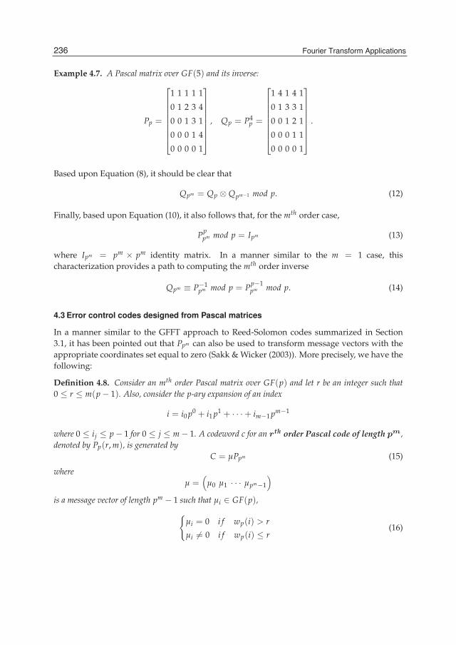
6 Will-be-set-by-IN-TECH
Example 4.7. A Pascal matrix over GF(5) and its inverse:
Pp =
⎡⎢⎢⎢⎢⎢⎢⎢⎣
1 1 1 1 1
0 1 2 3 4
0 0 1 3 1
0 0 0 1 4
0 0 0 0 1
⎤⎥⎥⎥⎥⎥⎥⎥⎦
, Qp = P4p =
⎡⎢⎢⎢⎢⎢⎢⎢⎣
1 4 1 4 1
0 1 3 3 1
0 0 1 2 1
0 0 0 1 1
0 0 0 0 1
⎤⎥⎥⎥⎥⎥⎥⎥⎦
.
Based upon Equation (8), it should be clear that
Qpm = Qp ⊗ Qpm−1 mod p. (12)
Finally, based upon Equation (10), it also follows that, for the mth order case,
Pppm mod p = Ipm (13)
where Ipm = pm × pm identity matrix. In a manner similar to the m = 1 case, thischaracterization provides a path to computing the mth order inverse
Qpm ≡ P−1pm mod p = Pp−1
pm mod p. (14)
4.3 Error control codes designed from Pascal matrices
In a manner similar to the GFFT approach to Reed-Solomon codes summarized in Section3.1, it has been pointed out that Ppm can also be used to transform message vectors with theappropriate coordinates set equal to zero (Sakk & Wicker (2003)). More precisely, we have thefollowing:
Definition 4.8. Consider an mth order Pascal matrix over GF(p) and let r be an integer such that0 ≤ r ≤ m(p − 1). Also, consider the p-ary expansion of an index
i = i0 p0 + i1 p1 + · · ·+ im−1 pm−1
where 0 ≤ ij ≤ p − 1 for 0 ≤ j ≤ m − 1. A codeword c for an rth order Pascal code of length pm,denoted by Pp(r, m), is generated by
C = μPpm (15)
whereμ =
(μ0 μ1 · · · μpm−1
)is a message vector of length pm − 1 such that μi ∈ GF(p),
{μi = 0 i f wp(i) > r
μi �= 0 i f wp(i) ≤ r(16)
236 Fourier Transform Applications

The Fourier Convolution Theorem over Finite Fields:Extensions of its Application to Error Control Codin 7
and
wp(i) ≡m−1
∑j=0
ij.
Error control codes derived from the mth order Pascal matrix over GF(2) (i.e. binary data) havebeen related (Forney (1988); Massey et al. (1973)) to a class of codes known as rth order binaryReed-Muller codes RM(r, m) of length 2m (MacWilliams & Sloane (1977); Wicker (1994)). Inaddition, it has been further demonstrated (Sakk (2002)) that P2(r, m) codes over GF(2) areequivalent to RM(r, m) codes with minimum distance dmin = 2m−r. These observations havebeen extended where it has been demonstrated that Pp(r, m) codes over GF(p) are equivalentto generalized Reed-Muller codes (GRM) codes (Sakk (2002)).
To place this class of codes in the same context as that outlined in Section 3.1, we mustshow how to introduce zeros into the message vector, apply the Pascal matrix as the lineartransformation and, based upon this transformation, introduce a convolution theorem. Fromthe definition above, a given code is specified by choosing p, m and a value of 0 ≤ r ≤m(p − 1). The code vector length then becomes n = pm; and, for this class of codes, a givenvalue of r defines the length k of the message. The rest of the n − k components of μ must beset to zero in a systematic way that leads to the minimum distance property of the code.
Example 4.9. Consider P23 in Example 4.2 (hence, n = 23 = 8) and a message vector μ =
(μ0, μ1, ..., μ7) and let s be the number of consecutive zeros in the vector μ for a given value ofr:
r = 0 (dmin = 8) : s = 7 μ = (μ0, 0, 0, 0, 0, 0, 0, 0) (k = 1)r = 1 (dmin = 4) : s = 3 μ = (μ0, μ1, μ2, 0, μ4, 0, 0, 0) (k = 4)r = 2 (dmin = 2) : s = 1 μ = (μ0, μ1, μ2, μ3, μ4, μ5, μ6, 0) (k = 7)r = 3 (dmin = 1) : s = 0 μ = (μ0, μ1, μ2, μ3, μ4, μ5, μ6, μ7) (k = 8)
Example 4.10. Consider P32 in Example 4.3 (hence, n = 32 = 9) and a message vector μ =
(μ0, μ1, ..., μ8) and let s be the number of consecutive zeros in the vector μ for a given value ofr:
r = 0 (dmin = 9) : s = 8 μ = (μ0, 0, 0, 0, 0, 0, 0, 0, 0) (k = 1)r = 1 (dmin = 6) : s = 5 μ = (μ0, μ1, 0, μ3, 0, 0, 0, 0, 0) (k = 3)r = 2 (dmin = 3) : s = 2 μ = (μ0, μ1, μ2, μ3, μ4, 0, μ6, 0, 0) (k = 6)r = 3 (dmin = 2) : s = 1 μ = (μ0, μ1, μ2, μ3, μ4, μ5, μ6, μ7, 0) (k = 8)r = 4 (dmin = 1) : s = 0 μ = (μ0, μ1, μ2, μ3, μ4, μ5, μ6, μ7, μ8) (k = 9)
In the above examples, dmin is shown in parentheses for each value of r; furthermore, observethat dmin = s + 1. Recalling for a moment the GFFT approach to Reed-Solomon code design,the minimum distance of a code where the message vector has n − k consecutive zeros canbe shown to be dmin = n − k + 1 (Blahut (2003); Wicker (1994)). It is apparent that, by usinga Pascal matrix as the transform, a result similar to that of the GFFT can be ascertained. Themajor difference is that, for Reed-Solomon codes, the string of zeros must occur at the end ofthe message vector before applying the GFFT to create C. For P(r, m), in addition to the stringof consecutive zeros, based upon the structure of Ppm , zeros must also be dispersed in otherpositions within μ to form code vectors C = μPpm .
237The Fourier Convolution Theorem over Finite Fields:Extensions of Its Application to Error Control Coding

8 Will-be-set-by-IN-TECH
5. Extensions of the Fourier convolution theorem over finite fields
The convolution operation involves relating the componentwise product of two vectors inone domain to the convolution of their transforms (Blahut & Burrus (1991)). Many lineartransforms have well-defined convolution operations. For instance, the Hadamard transformyields the so-called logical or ’dyadic’ convolution operation (Ahmed et al. (1973); Dodd(2003); Robinson (1972)). In this chapter, we develop extensions of the convolution theoremthat can be used to reveal useful properties of other classes of codes. As an example, wedemonstrate how the GFFT approach can be applied to describe generalized Reed-Mullercodes (Blahut (2003)).
To begin the formulation, we consider the componentwise product γj = μjλj of two vectorsμ = (μ0 ... μn−1) and λ = (λ0 ... λn−1). Furthermore, we consider matrix transforms such thatC ≡ μPpm and Λ ≡ λPpm or, equivalently, μ = CQpm and λ = ΛQpm where (Ppm )−1 ≡ Qpm .(here, ’μ’ denotes the message vector and ’C’ denotes the code vector). We demonstrate aformulation analogous to the convolution operation that describes γ = ΓQpm :
Γi =n−1
∑j=0
γj pji mod p i = 0, 1, ..., n − 1
=n−1
∑j=0
(μjλj)pji mod p
=n−1
∑j=0
μj(n−1
∑k=0
Λkqkj)pji mod p
=n−1
∑k=0
Λk(n−1
∑j=0
μjqkj pji) mod p
≡n−1
∑k=0
ΛkTi,k mod p i = 0, 1, ..., n − 1
(17)
where n = pm.
Notice that if we are dealing with familiar spectral transforms such as the Fourier or theHadamard transform (where P denotes the forward transform and Q denotes the inversetransform), Ti,k takes on a simple form. This is because the product qkj pji in ∑n−1
j=0 μjqkj pji
reduces to a term that enables us to take the transform of μ as Cf (i,k) = 1n (∑
n−1j=0 μj pj, f (i,k)).
For the case of the Fourier transform f (i, k) = i − k and Ti,k = C(i−k); as expected, one endsup with the convolution theorem (Blahut (2003); Wicker (1994)). In the case of a Hadamardtransform, f (i, k) = i ⊕ k (where ⊕ denotes bit-by-bit addition of the binary expansions of iand k) and Ti,k = C(i⊕k). Here, the bit-by-bit addition ⊕ of the binary expansions of i and kover GF(2) would result in the dyadic convolution (Ahmed et al. (1973); Robinson (1972)).
For the codes in this presentation, the qkj pji term in the above summation leads to aconvolution theorem that depends on the matrix Ppm . Furthermore, this theorem can alsobe applied to demonstrate how to decode C to recover the message vector μ. In Equation (17)
238 Fourier Transform Applications

The Fourier Convolution Theorem over Finite Fields:Extensions of its Application to Error Control Codin 9
qkj = (−1)j−k( jk) mod p and pji = (i
j) mod p; therefore, the product qkj pji will not lead to anexpression that readily reduces the inner summation to a single term. To see why, let’s writeout Ti,k as follows:
Ti = (Ti,0 Ti,1 ... Ti,n−1)
= (μ0 μ1 ... μn−1)
⎡⎢⎢⎢⎢⎣
q00 p0i q10 p0i · · · q(n−1)0 p0iq01 p1i q11 p1i · · · q(n−1)1 p1i
...... · · · ...
q0(n−1)p(n−1)i q1(n−1)p(n−1)i · · · q(n−1)(n−1)p(n−1)i
⎤⎥⎥⎥⎥⎦
= (μ0 μ1 ... μn−1)
⎡⎢⎢⎢⎢⎣
p0ip1i
. . .p(n−1)i
⎤⎥⎥⎥⎥⎦
⎡⎢⎢⎢⎢⎣
q00 q10 · · · q(n−1)0q01 q11 · · · q(n−1)1
...... · · · ...
q0(n−1) q1(n−1) · · · q(n−1)(n−1)
⎤⎥⎥⎥⎥⎦
≡ μDiQTpm
(18)
where T denotes the matrix transpose.
Observation 5.1. The components of the vector Ti = (Ti,0 Ti,1 ... Ti,n−1) can be written as a linearcombination of the components of C = (C0 ... Cn−1).
Proof: LetMi ≡ DiQT
pm (19)
where Di is defined in Equation (18) and
Ai ≡ Qpm Mi = Qpm DiQTpm
⇒ Mi = Ppm Ai.(20)
Then,Ti = μMi = μPpm Ai = CAi. (21)
Combining this result with Equation (17) we conclude
Γi =n−1
∑k=0
ΛkTi,k mod p i = 0, 1, ..., n − 1
=n−1
∑k=0
Λk(CAi)k mod p i = 0, 1, ..., n − 1
(22)
So, instead of Ti,k reducing to one single component of the vector C (as one might expectfrom a typical convolution operation), the Pascal convolution requires a linear combination ofthe components of C. Although this operation is slightly more complicated than the Fourierapproach, the identity in Equation (8) does induce a simplification.
Observation 5.2. (Symbolic Computation of Pascal Convolution)For the 1st order case where n = p and i = 0, ..., p − 1, using Equation (19) let Mi ≡ Mi,
239The Fourier Convolution Theorem over Finite Fields:Extensions of Its Application to Error Control Coding

10 Will-be-set-by-IN-TECH
using Equation (18) let Di ≡ Di and let Ai ≡ Qp Mi. Then, for any 0 ≤ j ≤ pm − 1 wherej = j0 p0 + j1 p1 + ... + jm−1 pm−1 and Aj = Qpm Mj,
Aj = Ajm−1 ⊗ ... ⊗ Aj1 ⊗ Aj0 (23)
where Mj ≡ DjQTpm .
Proof: The statement is clearly true for the first order case m = 1 since j = j0. By inductionlet j = j0 p0 + j1 p1 + ... + jm−1 pm−1 and assume that
Dj = Djm−1 ⊗ ... ⊗ Dj1 ⊗ Dj0
where 0 ≤ jk ≤ p − 1 for all k = 0, ..., m − 1. Consider any j′ = j0 p0 + ... +jm−1 pm−1 + jm pm and apply Equation (18) along with Lucas’ theorem to obtain thefollowing intermediate result:
Djm ⊗ Djm−1⊗... ⊗ Dj0 = Djm ⊗ Dj
=
⎡⎢⎢⎢⎢⎢⎣
(jm0 )
(jm1 )
. . .
( jmp−1)
⎤⎥⎥⎥⎥⎥⎦⊗
⎡⎢⎢⎢⎢⎢⎣
( j0)
( j1)
. . .
( jpm−1)
⎤⎥⎥⎥⎥⎥⎦
=
⎡⎢⎢⎢⎢⎢⎣
(j′0)
(j′1)
. . .
(j′
pm+1−1)
⎤⎥⎥⎥⎥⎥⎦
= Dj′
(24)
Therefore, Dj = Djm−1 ⊗ ...⊗ Dj1 ⊗ Dj0 is true. Next, successively apply the identity (AC)⊗(BD) = (A ⊗ B)(C ⊗ D) to obtain:
Mjm−1 ⊗ ... ⊗ Mj1 ⊗ Mj0 = (Djm−1 QTp )⊗ ... ⊗ (Dj1 QT
p )⊗ (Dj0 QTp )
= (Djm−1 ⊗ ... ⊗ Dj1 ⊗ Dj0 )(QTp ⊗ QT
p ⊗ ... ⊗ QTp )
= DjQTpm
= Mj
Finally, we arrive at the desired conclusion
(Ajm−1 ⊗ ... ⊗ Aj1 ⊗ Aj0 ) = (Qp Mjm−1 )⊗ ... ⊗ (Qp Mj1 )⊗ (Qp Mj0 )
= (Qp ⊗ Qp ⊗ ...Qp)(Mjm−1 ⊗ ... ⊗ Mj1 ⊗ Mj0 )
= Qpm Mj
= Aj.
240 Fourier Transform Applications

The Fourier Convolution Theorem over Finite Fields:Extensions of its Application to Error Control Codin 11
Observation 5.2 tells us that, in order to calculate Tj = CAj for arbitrary n = pm, one needonly calculate Ai for i = 0, ..., p − 1 and then take successive Kronecker products. The initialset of Ai for i = 0, ..., p − 1 can easily be calculated by referring back to Equation (20) whereAi = Qp Mi = QpDiQT
p .
An interesting property concerning the Ai is that the sum
pm−1
∑i=0
Ai =pm−1
∑i=0
QpDiQTp
(where the sum is taken mod p) is a matrix of ones. This follows from two observations. First,from the definition of Di in Equation (18), ∑
pm−1i=0 Di is a matrix whose (pm − 1, pm − 1) entry
is one and all other entries are zero. Second, it can also be demonstrated that the last columnof Qpm must be a column of ones. Therefore, Qp ∑
pm−1i=0 DiQT
p = ∑pm−1i=0 Ai is a matrix of ones.
Example 5.3. For p = 2, the 1st order case n = p gives i = 0, 1; hence, over GF(2),
Pp =
[1 10 1
], Qp = Pp =
[1 10 1
],
we calculate
A0 = QpD0QTp =
[1 10 1
] [1 00 0
] [1 01 1
]=
[1 00 0
]
A1 = QpD1QTp =
[1 10 1
] [1 00 1
] [1 01 1
]=
[0 11 1
].
From Observation 5.2, to obtain the Aj for n = p2 and j = 0, 1, 2, 3, one need only take successiveKronecker products as:
A0 = A0 ⊗ A0 =
⎡⎢⎢⎣
1 0 0 00 0 0 00 0 0 00 0 0 0
⎤⎥⎥⎦ , A1 = A0 ⊗ A1 =
⎡⎢⎢⎣
0 1 0 01 1 0 00 0 0 00 0 0 0
⎤⎥⎥⎦ ,
A2 = A1 ⊗ A0 =
⎡⎢⎢⎣
0 0 1 00 0 0 01 0 1 00 0 0 0
⎤⎥⎥⎦ , A3 = A1 ⊗ A1 =
⎡⎢⎢⎣
0 0 0 10 0 1 10 1 0 11 1 1 1
⎤⎥⎥⎦ .
As expected, the Ai are symmetric matrices. Also, notice, as mentioned above, that ∑pm−1i=0 Ai is a
matrix of ones. For the case where n = p2, let us now apply Observation 5.1 to calculate the Pascalconvolution of the vectors C = (C0, C1, C2, C3) and Λ = (Λ0, Λ1, Λ2, Λ3). Using Equation (22), wehave:
Γ0 = Λ0C0 + Λ1(0) + Λ2(0) + Λ3(0)Γ1 = Λ0C1 + Λ1(C0 + C1) + Λ2(0) + Λ3(0)Γ2 = Λ0C2 + Λ1(0) + Λ2(C0 + C2) + Λ3(0)Γ3 = Λ0C3 + Λ1(C2 + C3) + Λ2(C1 + C3) + Λ3(C0 + C1 + C2 + C3).
(25)
241The Fourier Convolution Theorem over Finite Fields:Extensions of Its Application to Error Control Coding

12 Will-be-set-by-IN-TECH
To close this section, we draw some immediate conclusions from Equation (25):
• Because of the Kronecker product, a good deal of self-similar structure can be observed inthe resulting vector Γ. For instance, the coefficients of the Λi can be computed by iterationstarting with the initial ’seed’ generated by A0 and A1. As an example, the coefficient ofΛ1 in Γ1 can be computed by adding the coefficient of Λ0 in Γ0 to the coefficient of Λ0 inΓ1. The coefficients of Λ2 and Λ3 in Γ2 and Γ3 can be computed by adding the coefficientsof Λ0 and Λ1 in Γ0 and Γ1 to the coefficients of Λ0 and Λ1 in Γ2 and Γ3, and so on.
• Looking at the result columnwise, the set of coefficients associated with a given Λi appearto be the checksums for an R(r, 2) binary Reed-Muller code ((MacWilliams & Sloane, 1977,p.385-388), (Wicker, 1994, p.155-165)). As pointed out in the next section, although thisobservation is true for the binary case, an orthogonal set of checksums for p > 2 will notcome about by this method. It is the dual of the Pascal convolution that will lead to thedecoding of GRM codes.
6. Majority logic decoding using Pascal convolution
GRM codes fall into a larger category of codes known as Euclidean geometry codes (Blahut(2003); Lin & Costello (1983); MacWilliams & Sloane (1977); Wicker (1994)) where it iswell-known that a technique known as ’majority logic decoding’ (MLD) can be used torecover the message vector. Based upon statements made in Section 4, it should be clearthat Pascal codes are also MLD. However, the role played by the Pascal convolution in thedecoding strategy is worthy of mention. As pointed out in the conclusions of Example 5.3, thechecksums of a majority logic decoding (MLD) scheme for GRM codes can be derived usingthe dual of the convolution relation derived above. We now demonstrate this observationmore clearly.
Because of the similar forms of Ppm and Qpm the dual convolution relation is easily derivedfrom the inverse transform. Consider the componentwise product Γj = CjΛj of two vectorswhere C = μPpm and Λ = λPpm :
γi =n−1
∑j=0
Γjqji mod p i = 0, 1, ..., n − 1
=n−1
∑j=0
(CjΛj)qji mod p
=n−1
∑j=0
Cj(n−1
∑k=0
λk pkj)qji mod p
=n−1
∑k=0
λk(n−1
∑j=0
Cj pkjqji) mod p
≡n−1
∑k=0
λksi,k mod p i = 0, 1, ..., n − 1
(26)
242 Fourier Transform Applications

The Fourier Convolution Theorem over Finite Fields:Extensions of its Application to Error Control Codin 13
where n = pm. Similar to Equation (18), one can also show that
si = (si,0 si,1 ... si,n−1)
= CΔiPTpm
(27)
which can also be written assi = μPpm ΔiPT
pm (28)
where Δi is a diagonal matrix with elements (q0i q1i ... q(n−1)i) along its diagonal.Furthermore, if we define
Bi ≡ Ppm ΔiPTpm (29)
then results similar to Observations 5.1 and 5.2 can also be demonstrated. However, inproving the dual of Observation 5.2 there is one difference be aware of. Since qji = (−1)i−j(i
j),
the Kronecker product in the dual of Equation (24) will contain extra factors of (−1)i−j. Toachieve the equality Δj = Δjm−1 ⊗ ... ⊗ Δj1 ⊗ Δj0 where j = j0 p0 + j1 p1 + ... + jm−1 pm−1 thefollowing identity will be required:
(−1)k = (−1)k0 p0+k1 p1+...+km−1 pm−1
= (−1)k0 ((−1)p)k1 ((−1)p2)k2 ...((−1)pm−1
)km−1
= (−1)∑m−1l=0 kl
for any 0 ≤ k ≤ pm − 1 where we have applied ap = a for any a ∈ GF(p). Then, followingthe proof of Observation 5.2, it is straightforward to show that for any 0 ≤ j ≤ pm − 1 wherej = j0 p0 + j1 p1 + ... + jm−1 pm−1,
Bj = Bjm−1 ⊗ ... ⊗ Bj1 ⊗ Bj0 (30)
whereBjk = PpΔjk PT
p .
In Section 4, we explained that the form of message vectors when applying Ppm as thetransformation where the message vector μ = (μ0, ..., μpm−1) should have all componentsμj = 0 if wp(j) > r (see Examples 4.9 and 4.10). To see how this formulation can lead to adecoding scheme, let us examine the case where p = 2, m = 2 and r = 1 (i.e. - a 1st orderbinary Reed-Muller code of length 4). Consider first using Equations (26) and (27) to calculatePascal convolution of the vectors μ = (μ0, μ1, μ2, μ3) and λ = (λ0, λ1, λ2, λ3):
00 : γ0 = λ0C0 + λ1(0) + λ2(0) + λ3(0)
01 : γ1 = λ0(C0 + C1) + λ1C1 + λ2(0) + λ3(0)
10 : γ2 = λ0(C0 + C2) + λ1(0) + λ2C2 + λ3(0)
11 : γ3 = λ0(∑3i=0 Ci) + λ1(C1 + C3) + λ2(C2 + C3) + λ3C3
. (31)
243The Fourier Convolution Theorem over Finite Fields:Extensions of Its Application to Error Control Coding
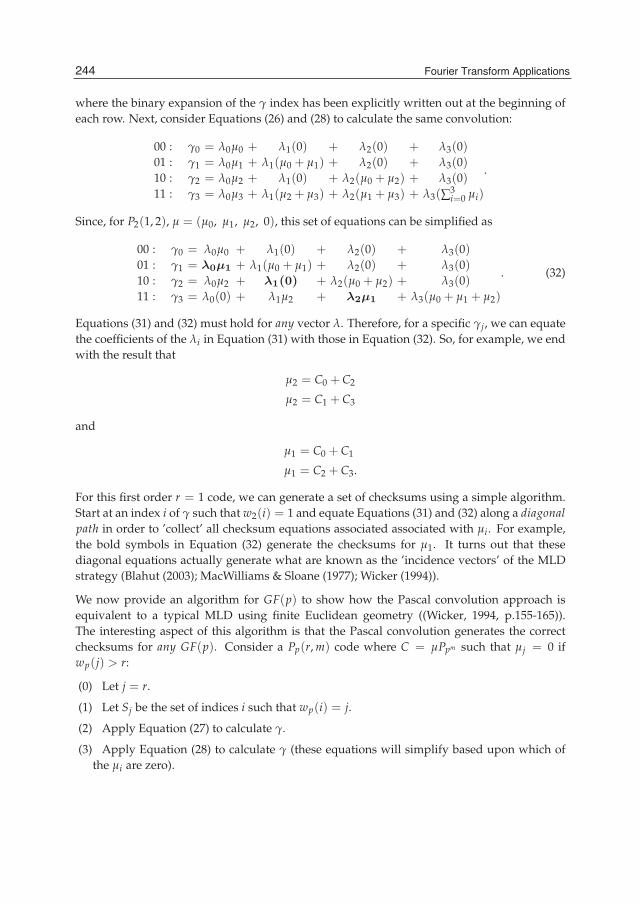
14 Will-be-set-by-IN-TECH
where the binary expansion of the γ index has been explicitly written out at the beginning ofeach row. Next, consider Equations (26) and (28) to calculate the same convolution:
00 : γ0 = λ0μ0 + λ1(0) + λ2(0) + λ3(0)01 : γ1 = λ0μ1 + λ1(μ0 + μ1) + λ2(0) + λ3(0)10 : γ2 = λ0μ2 + λ1(0) + λ2(μ0 + μ2) + λ3(0)11 : γ3 = λ0μ3 + λ1(μ2 + μ3) + λ2(μ1 + μ3) + λ3(∑3
i=0 μi)
.
Since, for P2(1, 2), μ = (μ0, μ1, μ2, 0), this set of equations can be simplified as
00 : γ0 = λ0μ0 + λ1(0) + λ2(0) + λ3(0)01 : γ1 = λ0μ1 + λ1(μ0 + μ1) + λ2(0) + λ3(0)10 : γ2 = λ0μ2 + λ1(0) + λ2(μ0 + μ2) + λ3(0)11 : γ3 = λ0(0) + λ1μ2 + λ2μ1 + λ3(μ0 + μ1 + μ2)
. (32)
Equations (31) and (32) must hold for any vector λ. Therefore, for a specific γj, we can equatethe coefficients of the λi in Equation (31) with those in Equation (32). So, for example, we endwith the result that
μ2 = C0 + C2
μ2 = C1 + C3
and
μ1 = C0 + C1
μ1 = C2 + C3.
For this first order r = 1 code, we can generate a set of checksums using a simple algorithm.Start at an index i of γ such that w2(i) = 1 and equate Equations (31) and (32) along a diagonalpath in order to ’collect’ all checksum equations associated associated with μi. For example,the bold symbols in Equation (32) generate the checksums for μ1. It turns out that thesediagonal equations actually generate what are known as the ’incidence vectors’ of the MLDstrategy (Blahut (2003); MacWilliams & Sloane (1977); Wicker (1994)).
We now provide an algorithm for GF(p) to show how the Pascal convolution approach isequivalent to a typical MLD using finite Euclidean geometry ((Wicker, 1994, p.155-165)).The interesting aspect of this algorithm is that the Pascal convolution generates the correctchecksums for any GF(p). Consider a Pp(r, m) code where C = μPpm such that μj = 0 ifwp(j) > r:
(0) Let j = r.
(1) Let Sj be the set of indices i such that wp(i) = j.
(2) Apply Equation (27) to calculate γ.
(3) Apply Equation (28) to calculate γ (these equations will simplify based upon which ofthe μi are zero).
244 Fourier Transform Applications

The Fourier Convolution Theorem over Finite Fields:Extensions of its Application to Error Control Codin 15
(4) For each i ∈ Sj, start at λ0 associated with γi and construct checksum equations byequating the result in Step (2) with that of Step (3) along a diagonal path (i.e. - starting atk=0, choose the coefficient of λk associated with γi+k).
(5) For i ∈ Sj, create estimates μi by a majority logic decision on the checksums.
(6) j = j − 1. If j < 0, stop.
(7) Remove the estimated components as:
C = μPpm
C ≡ C − C (= (μ − μ)Ppm ).
(8) Adjust μ to reflect the change in step (7) as follows. Construct a new vector μ whereμi = μi if i ∈ Sj and μi = 0 otherwise. Then let
μ ≡ μ − μ.
(9) Let C = C and μ = μ and go to Step (1).
As with typical MLD schemes, this algorithm starts with the highest order r to obtain estimatesof the code vector components and then successively estimates the lower order components.
Example 6.1. Let p = 3, m = 2 and r = 2. Consider decoding a P3(2, 2) code. From Example 4.10,
μ = (μ0, μ1, μ2, μ3, μ4, 0, μ6, 0, 0).
Also, we know that P3(2, 2) has dmin = 3 implying that we can correct a single error. Therefore, weexpect that the MLD equations should have at least three checksums.
(0) Start with j = 2.
(1) Let S2 = {2, 4, 6} (i.e. - i = i0 + i1 p such that w3(i) = 2).
(2,3,4) Rather than write out the equations for γi , we summarize by equating the results of step (2)and step (3):
i = 2 :
μ2 = c0 + c1 + c2
μ2 = c3 + c4 + c5
μ2 = c6 + c7 + c8
i = 4 :
μ4 = c0 + 2c1 + 2c3 + c4
2μ4 = 2c1 + c2 + c4 + 2c5
2μ4 = 2c3 + c4 + c6 + 2c7
μ4 = c4 + 2c5 + 2c7 + c8
i = 6 :
μ6 = c0 + c3 + c6
μ6 = c1 + c4 + c7
μ6 = c2 + c5 + c8
245The Fourier Convolution Theorem over Finite Fields:Extensions of Its Application to Error Control Coding

16 Will-be-set-by-IN-TECH
After estimating the message components dictated by S2 (step (5)), remove the code estimates fromC (step (7)) and begin work on S1 where now (step(8)) μi = 0 if wp(i) > 1. For S1, we have thechecksums:
i = 1 :
μ1 = 2c0 + c1
2μ1 = c1 + 2c2
μ1 = 2c3 + c4
2μ1 = c4 + 2c5
μ1 = 2c6 + c7
2μ1 = c7 + 2c8
i = 3 :
μ3 = 2c0 + c3
μ3 = 2c1 + c4
μ3 = 2c2 + c5
2μ3 = c3 + 2c6
2μ3 = c4 + 2c7
2μ3 = c5 + 2c8
After estimating the message components dictated by S1, once again, remove the code estimates fromC and begin work on S0 where now μi = 0 if wp(i) > 0. At this stage, with all other components ofμ = 0 except μ0, we are left with μ = C (i.e. - nine estimate of the check on μ0).
7. Conclusions
When considering the design of error control codes, it is interesting to look for guidingprinciples that can account for whole classes of codes. In this presentation, we have shownhow the GFFT convolution approach to Reed-Solomon codes can be extended to other classesof codes such as generalized Reed-Muller codes.
Code Convolution Principle Decoding StrategyReed-Solomon GFFT-based iterative
GRM generalized iterative
Table 1. Comparison of Fourier and generalized convolution techniques.
Instead of applying a Fourier matrix to encode the message, we have applied a Pascal matrixand extended the convolution theorem over finite fields. In doing so, we have observedthat this formulation leads to the well-known majority logic decoding algorithm. Additionalinvestigations have also considered codes in the context of the wavelet transform (Sakk& Wicker (2003)). The block codes addressed in this chapter have been shown to lendthemselves to graph-based iterative decoding strategies (see Table 1). The results derivedabove suggest that the generalized convolution approach is useful for understanding thesystematic introduction of redundancy for the sake of error control.
246 Fourier Transform Applications

The Fourier Convolution Theorem over Finite Fields:Extensions of its Application to Error Control Codin 17
8. References
Ahmed, N., Rao, K. & Abdussattar, A. (1973). On cyclic autocorrelation and theWalsh-Hadamard transform, IEEE Transactions on Electromagnetic Compatibility18: 141–146.
Blahut, R. (2003). Algebraic Codes for Data Transmission, Cambridge University Press.Blahut, R. & Burrus, C. (1991). Algebraic Methods for Signal Processing and Communications
Coding, Springer.Burrus, C., Gopinath, R. & Guo, H. (1998). Introduction to Wavelets and Wavelet Transforms,
Prentice-Hall, NJ.Caire, G., Grossman, R. & Poor, H. (1993). Wavelet transforms and associated finite cyclic
groups, IEEE Transactions on Information Theory 39: 1157–1166.Call, G. & Velleman, D. (1993). Pascal’s matrices, American Mathematical Monthly 100: 372–376.Dodd, M. (2003). Applications of the Discrete Fourier Transform in Information Theory and
Cryptology, PhD thesis, Royal Holloway and Bedford New College, University ofLondon.
Forney, G. D. (1988). Coset codes - Part II: Binary lattices and related codes, IEEE Transactionson Information Theory 34: 1152–1187.
Heller, S. (1963). Inverse of triangular matrix, American Mathematical Monthly 70: 334.Kou, Y., Lin, S. & Fossorier, M. P. C. (2001). Low-density parity-check codes based on finite
geometries: A rediscovery and new results, IEEE Transactions on Information Theory47: 2711–2736.
Li, G., Li, D., Wang, Y. & Sun, W. (2010). Hybrid decoding of finite geometry low-densityparity-check codes, IET Communications 4(10): 1238–1246.
Lin, S. & Costello, D. (1983). Error Control Coding: Fundamentals and Applications, Prentice-Hall,New York.
Liu, Z. & Pados, D. A. (2005). Decoding algorithm for finite-geometry LDPC codes, IEEETransactions on Communications 53: 415–421.
MacWilliams, F. J. & Sloane, N. J. A. (1977). The Theory of Error-Correcting Codes,North-Holland, Amsterdam.
Massey, J. L., Costello, D. J. & Justesen, J. (1973). Polynomial weights and code constructions,IEEE Transactions on Information Theory 19: 101–110.
Ngatched, T. M. N., F, T. & Bossert, M. (2009). An improved decoding algorithm forfinite-geometry LDPC codes, IEEE Transactions on Communications 57: 302–306.
O.Vontobel, P., Smarandache, R., Kiyavash, N., Teutsch, J. & D.Vukobratovic (2005). On theminimal pseudocodewords of codes from finite geometries, Proc. IEEE Int. Symp. Inf.Theory, Adelaide, Australia.
Pusane, A. E., Smarandache, R., Vontobel, P. O. & Costello, D. J. (2011). Deriving good LDPCconvolutional codes from LDPC block codes, IEEE Transactions on Information Theory57: 835–857.
Robinson, G. (1972). Logical convolution and discrete Walsh and Fourier power spectra, IEEETransactions on Audio and Electroacoustics 20: 271–280.
Sakk, E. (2002). Wavelet Packet Formulation of Generalized Reed Muller Codes, PhD thesis, CornellUniversity, Ithaca, NY.
247The Fourier Convolution Theorem over Finite Fields:Extensions of Its Application to Error Control Coding
18 Will-be-set-by-IN-TECH
Sakk, E. & Wicker, S. (2003). Wavelet packets for error control coding, Proceedings of the SPIEVolume 5207 (Wavelets X), San Diego, CA.
Smarandache, R., Pusane, A. E., Vontobel, P. O. & Costello, D. J. (2009). Pseudocodewordperformance analysis for LDPC convolutional codes, IEEE Transactions on InformationTheory 55: 2577–2598.
Strang, G. & Nuygen, T. (1996). Wavelets and Filter Banks, Wellesley-Cambridge Press,Wellesley, MA.
Tang, H., Xu, J., Lin, S. & Abdel-Ghaffar, K. A. S. (2005). Codes on finite geometries, IEEETransactions on Information Theory 51: 572–596.
Vandendriesscher, P. (2010). Some low-density parity-check codes derived from finitegeometries, Designs, Codes and Cryptography 54: 287–297.
Wicker, S. (1994). Error Control Systems for Digital Communication and Storage, Prentice Hall.Wicker, S. & Kim, S. (2003). Fundamentals of codes, graphs, and iterative decoding, Kluwer.Xia, S.-T. & Fu, F.-W. (2008). Minimum pseudoweight and minimum pseudocodewords of
LDPC codes, IEEE Transactions on Information Theory 54: 480–485.Zhang, L., Huang, Q. & Lin, S. (2010). Iterative decoding of a class of cyclic codess, Information
Theory and Applications Workshop (ITA), San Diego, CA.
248 Fourier Transform Applications

0
Application of the Weighted Energy Method in thePartial Fourier Space to Linearized Viscous
Conservation Laws with Non-Convex ConditionYoshihiro Ueda
Faculty of Maritime Sciences, Kobe UniversityJapan
1. Introduction
As you know, the energy method in the Fourier space is useful in deriving the decay estimatesfor problems in the whole space Rn. Recently, the author studied half space problems in Rn
+ =
R+ × Rn−1 and developed the energy method in the partial Fourier space obtained by takingthe Fourier transform with respect to the tangential variable Rn−1. Then the author appliedthis energy method to the half space problem for linearized viscous conservation laws withconvex condition and proved the asymptotic stability of planar stationary waves by showinga sharp convergence rate for t → ∞ (see, [14]).
In this chapter, we consider the half space problem for linearized viscous conservation lawswith non-convex condition, and derive the asymptotic stability of planar stationary waves andthe corresponding convergence rate. Our proof is based on the energy method in the partialFourier space with the anti-derivative method.
In this present chapter, we are concerned with the half space problem for the viscousconservation laws:
ut − Δu +∇ · f (u) = 0, (1.1)
u(0, x′, t) = ub, (1.2)
u(x, 0) = u0(x). (1.3)
Here x = (x1, · · · , xn) is the space variable in the half space Rn+ = R+ × Rn−1 with n ≥ 2;
we sometimes write as x = (x1, x′) with x1 ∈ R+ and x′ = (x2, · · · , xn) ∈ Rn−1; u(x, t) is theunknown function, u0(x) is the initial data satisfying
u0(x) → 0 as x1 → ∞,
and ub is the boundary data (assumed to be a constant) with ub < 0; f (u) = ( f1(u), · · · , fn(u))is a smooth function of u ∈ R with values in Rn and satisfies
f1(0) = 0, f1(u) > f1(0) (= 0) (1.4)
for u ∈ [ub, 0). Here we note that the condition (1.4) is the necessary condition for theexistence of the planar stationary waves (for the detail, see Section 2.2). We emphasize that
10

2 Will-be-set-by-IN-TECH
the assumption (1.4) is weaker than the convex condition
f ′′1 (u) > 0 (1.5)
for u ∈ [ub, 0] and f1(0) = 0. Namely, we do not assume the convex condition for our problem(1.1)–(1.3).
For viscous conservation laws (1.1) with the convex condition (1.5), there are many results onthe asymptotic stability of nonlinear waves. First, Il’in and Oleinik in [3] studied the stabilityof nonlinear waves in the one-dimensional whole space. Liu, Matsumura and Nishiharain the paper [8] discussed the stability of stationary waves in one-dimensional half space.More precisely, they proved the asymptotic stability of several kind of nonlinear wavessuch as rarefaction waves, stationary waves, and the superposition of stationary waves andrarefaction waves. Later, in a series of papers [5–7], their stability result of stationary waves inone-space dimension was generalized to the multi-dimensional case. Kawashima, Nishibataand Nishikawa [5] first considered the stability of non-degenerate planar stationary wavesin two-dimensional half space and obtained the convergence rate t−1/4−α/2 in L∞ norm byassuming that the initial perturbation is in L2
α(R+; L2(R)). Furthermore, the papers [6, 7]studied the n-dimensional problem in the Lp framework. In particular, the paper [7] showedthe stability of non-degenerate planar stationary waves and obtained the convergence ratet−(n/2)(1/2−1/p)−α/2 in Lp norm under the assumption that the initial perturbation belongs toL2
α(R+; L2x′ ).
Next, we refer to viscous conservation laws with non-convex condition. Liu and Nishiharain [9] and Nishikawa in [10] investigated the asymptotic stability of travelling waves inthe one-dimensional and multi-dimensional whole space, respectively. On the other hand,Hashimoto and Matsumura in [1] studied the asymptotic stability of stationary waves inthe one-dimensional half space. Especially, in order to relax the convex condition, Liu andNishihara in [9] and Nishikawa in [10] employed the anti-derivative method and achieved thedesired result. Moreover, Hashimoto and the author in [2] used the same method to derivethe asymptotic stability of stationary waves for damped wave equations with non-convexconvection term in one-dimensional half space. Inspired by these arguments, we try torelax the convex condition (1.5) and get the asymptotic stability of planar stationary wavefor the multi-dimensional problem (1.1)–(1.3). Unfortunately, Nishikawa in the paper [10]considered some special situation for the nonlinear term to make a good combination of theenergy method and the anti-derivative method. For the same reason, we will treat the specialsituation (for the detail, see Section 3).
All these stability results mentioned above are obtained by employing the energy method inthe physical space. On the other hand, it is useful to apply the energy method in the partialFourier space to show sharper convergence rate. Indeed the author’s paper [14] consideredour problem (1.1)–(1.3) with the convex condition (1.5) and obtained the sharper convergencerate of the planar stationary waves. We shall show the result of the paper [14] in detail.
We are interested in the asymptotic stability of one-dimensional stationary solution φ(x1)(called planar stationary wave) for the problem (1.1)–(1.3): φ(x1) is a solution to the problem
−φx1x1 + f1(φ)x1 = 0, (1.6)
φ(0) = ub, φ(x1) → 0 as x1 → ∞. (1.7)
250 Fourier Transform Applications

Application of the Weighted Energy Method in the Partial Fourier Space to Linearized Viscous Conservation Laws with Non-Convex Condition 3
To show the stability, it is convenient to introduce the perturbation v and write the solution uin the form
u(x, t) = φ(x1) + v(x, t).
The original problem (1.1)–(1.3) is then reduced to
vt − Δv +∇ · ( f (φ + v)− f (φ)) = 0, (1.8)
v(0, x′, t) = 0, (1.9)
v(x, 0) = v0(x), (1.10)
where v0(x) = u0(x)− φ(x1); notice that v0(x) → 0 as x1 → ∞.
Under the convex condition (1.5), the author in [14] showed the asymptotic stability of theplanar stationary wave φ(x1) by proving a sharp decay estimate for the perturbation v(x, t).To this end we employed the energy method in the partial Fourier space Rn
+ = R+ × Rn−1ξ
which is obtained by taking the Fourier transform with respect to the tangential variable x′ =(x2, · · · , xn) ∈ Rn−1; ξ = (ξ2, · · · , ξn) ∈ Rn−1
ξ is the Fourier variable corresponding to x′ ∈Rn−1. For the variable x1 ∈ R+ in the normal direction, we use L2 space (or weighted L2
space). As the result, for the corresponding linearized problem with f (φ + v)− f (φ) replacedby f ′(φ)v in (1.8), we showed the following pointwise estimate with respect to ξ ∈ Rn−1
ξ :
|Fv(·, ξ, t)|L2 ≤ Ce−κ|ξ|2t|Fv0(·, ξ)|L2 , (1.11)
where C and κ are positive constants. Here F denotes the Fourier transform with respect tox′ ∈ Rn−1 and | · |L2 is the L2 norm with respect to x1 ∈ R+. This pointwise estimate (1.11)enables us to get the following sharp decay estimate:
‖v(t)‖L2 ≤ Ct−(n−1)/4‖v0‖L2(L1), (1.12)
where ‖ · ‖L2 denotes the L2 norm with respect to x = (x1, x′) ∈ Rn+, ‖ · ‖L2(L1) is the norm in
L2(R+; L2x′ ∩ L1
x′ ), and C is a positive constant.
Furthermore, when the planar stationary wave φ(x1) is non-degenerate, the author appliedthe weighted energy method in the partial Fourier space Rn
+ = R+ × Rn−1ξ . Namely, we used
the weighted space L2α with respect to x1 ∈ R+. In this case, the pointwise estimate (1.11) is
improved to|Fv(·, ξ, t)|L2 ≤ C(1 + t)−α/2e−κ|ξ|2t|Fv0(·, ξ)|L2
α, (1.13)
where | · |L2α
denotes the L2α norm with respect to x1 ∈ R+. Consequently, we had the decay
estimate‖v(t)‖L2 ≤ C(1 + t)−α/2t−(n−1)/4‖v0‖L2
α(L1), (1.14)
where ‖ · ‖L2α(L1) is the norm in L2
α(R+; L2x′ ∩ L1
x′ ). For the above results, we refer to the reeder[14] in detail.
The main purpose of this chapter is to derive the sharp decay estimate (1.11)–(1.14) for thelinearized problem of (1.8)–(1.10) with non-convex condition (1.4), i.e.,
vt − Δv +∇ · ( f ′(φ)v) = 0 (1.15)
251Application of the Weighted Energy Method in the Partial Fourier Space to Linearized Viscous Conservation Laws with Non-Convex Condition

4 Will-be-set-by-IN-TECH
with (1.9), (1.10). To overcome the difficulty occured by the non-convex condition, we makea good combination of the weighted energy method in partial Fourier space employed in [14]and the anti-derivative method employed in [2, 9], and get the desired results. Once we obtainthe linear stability results for the problem (1.15), (1.9), (1.10), we may apply this results to theasymptotic stability for the nonlinear problem (1.8)–(1.10).
The remainder of this chapter is organized as follows. In Section 2, we introduce functionspaces and some preliminaries used in this chapter. Especially, we reformulate our problem(1.15), (1.9), (1.10) by using the anti-derivative method in Section 2.3. In the final section,we treat the half space problem for the reformulated viscous conservation laws and (1.15),(1.9), (1.10), and develop the weighted energy method in the partial Fourier space with theanti-derivative method. In this section, we derive pointwise estimates of solutions and provethe corresponding decay estimates.
2. Preliminaries
2.1 Notations and function spaces
Let us consider functions defined in the half space Rn+ = R+ ×Rn−1. We sometimes write the
space variable x = (x1, · · · , xn) ∈ Rn+ as x = (x1, x′) with x1 ∈ R+ and x′ = (x2, · · · , xn) ∈
Rn−1. The symbols ∇ = (∂x1 , · · · , ∂xn ) and Δ = ∑nj=1 ∂2
xjdenote the standard gradient and
Laplacian with respect to x = (x1, . . . , xn), respectively. The symbol ∇x′ = (∂x2 , · · · , ∂xn )denotes the gradient of the tangential direction with respect to x = (x2, . . . , xn). Thus wehave ∇ · g = ∑n
j=1 ∂xj gj for g = (g1, · · · , gn), and ∇x′ · g∗ = ∑nj=2 ∂xj gj for g∗ = (g2, · · · , gn).
Let v(x1, ξ) be the Fourier transform of v(x1, x′) with respect to x′ ∈ Rn−1:
v(x1, ξ) = F [v(x1, ·)](ξ) = (2π)−(n−1)/2∫
Rn−1v(x1, x′)e−ix′ ·ξ dx′, (2.1)
where ξ = (ξ2, · · · , ξn) ∈ Rn−1ξ is the Fourier variable corresponding to x′ = (x2, · · · , xn) ∈
Rn−1 and x′ · ξ = ∑nj=2 xjξ j.
Let 1 ≤ p ≤ ∞. We denote by Lpx′ = Lp(Rn−1) the Lp space with respect to x′ ∈ Rn−1, with
the norm ‖ · ‖Lpx′
. For a nonnegative integer s, we denote by Hsx′ = Hs(Rn−1) the Sobolev
space over Rn−1 with the norm
‖v‖Hsx′=
( s
∑k=0
‖∂kx′v‖2
L2x′
)1/2,
where ∂kx′ denotes the totality of all the k-th order derivatives with respect to x′ ∈ Rn−1. Also,
we denote by Lp(R+) the Lp space with respect to x1 ∈ R+, with the norm | · |Lp . For anonnegative integer s, we denote by Hs(R+) the Sobolev space over R+, with the norm | · |Hs .For α ∈ R, we denote by L2
α(R+) the weighted L2 space over R+ with the norm
|v|L2α=
( ∫ ∞
0(1 + x1)
α|v(x1)|2dx1
)1/2.
Now we introduce function spaces over the half space Rn+ = R+ × Rn−1. Let 1 ≤ p, q ≤ ∞, s
be a nonnegative integer, and α ∈ R. The space Lq(Lp) = Lq(R+; Lpx′ ) consists of Lq functions
252 Fourier Transform Applications

Application of the Weighted Energy Method in the Partial Fourier Space to Linearized Viscous Conservation Laws with Non-Convex Condition 5
of x1 ∈ R+ with values in Lpx′ with respect to x′ ∈ Rn−1. The norm is denoted by ‖ · ‖Lq(Lp).
When q = p, we simply write as
Lp = Lp(Lp), ‖ · ‖Lp = ‖ · ‖Lp(Lp).
The space Hs(Lp) = Hs(R+; Lpx′ ) consists of Hs functions of x1 ∈ R+ with values in Lp
x′ withrespect to x′ ∈ Rn−1. The norm is denoted by ‖ · ‖Hs(Lp). Also, L2
α(Lp) = L2α(R+; Lp
x′ ) denotesthe space of L2
α functions of x1 ∈ R+ with values in Lpx′ with respect to x′ ∈ Rn−1. The norm
is denoted by
‖v‖L2α(Lp) =
( ∫ ∞
0(1 + x1)
α‖v(x1, ·)‖2Lp
x′dx1
)1/2.
We sometimes useL2
α = L2α(L2), ‖ · ‖L2
α= ‖ · ‖L2
α(L2).
L2(Hs) = L2(R+; Hsx′ ) denotes the space of L2 functions of x1 ∈ R+ with values in Hs
x′ withrespect to x′ ∈ Rn−1, whose norm is given by
‖v‖L2(Hs) =( ∫ ∞
0‖v(x1, ·)‖2
Hsx′
dx1
)1/2
=( s
∑k=0
∫ ∞
0‖∂k
x′v(x1, ·)‖2L2
x′dx1
)1/2=
( s
∑k=0
‖∂kx′v‖2
L2
)1/2.
By the definition (2.1) of the Fourier transform, we see that
supξ∈Rn−1
ξ
|v(·, ξ)|L2 ≤ C‖v‖L2(L1) (2.2)
with C = (2π)−(n−1)/2. Also, it follows from the Plancherel theorem that
‖∂kx′v‖L2
α=
( ∫Rn−1
ξ
|ξ|2k|v(·, ξ)|2L2αdξ
)1/2. (2.3)
Let T > 0 and let X be a Banach space defined on the half space Rn+. Then C([0, T]; X) denotes
the space of continuous functions of t ∈ [0, T] with values in X.
In this paper, positive constants will be denoted by C or c.
2.2 Stationary solution
We review the results on the stationary problem (1.6)–(1.7). For the details, we refer the readerto [2, 8, 11–13].
Proposition 2.1 ([8]). Assume the condition (1.4). Then f ′1(0) ≤ 0 is necessary for the existence ofsolutions to the stationary problem (1.6)–(1.7). Conversely, under the condition f ′1(0) ≤ 0, we havethe following existence result:
(i) Non-degenerate case where f ′1(0) < 0: In this case the stationary problem (1.6)–(1.7) admits aunique smooth solution φ(x1) with φx1 > 0 (resp. φx1 < 0), provided that ub < 0 (resp. 0 < ub andf1(u) < f1(0) for 0 < u < ub). The solution verifies
|φ(x1)| ≤ Ce−cx1 , x1 > 0,
253Application of the Weighted Energy Method in the Partial Fourier Space to Linearized Viscous Conservation Laws with Non-Convex Condition

6 Will-be-set-by-IN-TECH
where C and c are positive constants.
(ii) Degenerate case where f ′1(0) = 0: In this case the problem (1.6)–(1.7) admits a unique smoothsolution φ(x1) if and only if ub < 0. The solution verifies φx1 > 0 and
|φ(x1)| ≤ C(1 + x1)−1/q, x1 > 0,
where q is the degeneracy exponent of f1 and C is a positive constant.
In this chapter we only treat the stationary solutions φ(x1) with φx1 > 0 and discusstheir stability; however, we must get the similar stability result of the monotone decreasingstationary solutions by using the same argument introduced in this chapter. (We refer thereader to [2].)
2.3 Reformulated problem
In this subsection we reformulate our problem by the anti-derivative method. To this end weintroduce a new function z(x, t) as
z(x, t) = −∫ ∞
x1
v(y, x′, t) dy. (2.4)
Here, we assume the integrability of v(x, t) over R+. This transformation is motivated bythe argument in Liu-Nishihara [9]. By using (2.4), we can reformulate (1.8)–(1.10) in terms ofz(x, t) as
zt − Δz + f ′(φ) · ∇z +∫ ∞
x1
φx1 f ′′∗ (φ) · ∇x′z dy = −g1 +∇x′ · h∗, (2.5)
zx1 (0, x′, t) = 0, (2.6)
z(x, 0) = z0(x), (2.7)
where z0(x) = − ∫ ∞x1(u0(y, x′) − φ(y))dy, f ′′∗ (φ) = ( f ′′2 (φ), · · · , f ′′n (φ)), and g1, ∇x′ · h∗ are
nonlinear terms defined by h∗ = (h2, · · · , hn) and
gj = f j(φ + zx1 )− f j(φ)− f ′j (φ)zx1 , hj =∫ ∞
x1
gj dy.
Once we obtain the solution for the problem (2.5)–(2.7), the differentiation v = zx1 is thesolution for (1.8)–(1.10). Namely, we will apply the weighted energy method in the partialFourier space and try ot derive the global solution in time to the reformulated problem(2.5)–(2.7). We will discuss this reformulated problem in Section 3 to prove our main theorems.
2.4 Weight function
We introduce the weight function employed in the weighted energy method. Our weightfunction is defined as
w(u) = (−eAu + 1)/ f1(u) for u ∈ [ub, 0], (2.8)
254 Fourier Transform Applications

Application of the Weighted Energy Method in the Partial Fourier Space to Linearized Viscous Conservation Laws with Non-Convex Condition 7
where A is a positive constant determined in Lemma 2.2. This weight function is veryimportant to derive a priori estimate in the latter section. For this weight function, we obtainthe following lemma.
Lemma 2.2 ([2]). Suppose that f1(u) satisfies (1.4). Let w(u) be the weight function defined in (2.8).Then there exists a positive constant δ such that if A ≥ δ, then w(u) satisfies the following conditions:
(i) (w f1)′(u) < 0 for u ∈ [ub, 0],
(ii) (w f1)′′(u) < 0 for u ∈ [ub, 0].
(2.9)
Moreover, let φ be the stationary solution constructed in Proposition 2.1. Then the weight functionsatisfies the following properties.
(i) Non-degenerate case where f ′1(0) < 0: The weight function w(φ) satisfies
c < w(φ) < C for φ ∈ [ub, 0].
(ii) Degenerate case where f ′1(0) = 0: The weight function w(φ) satisfies
c(1 + x1) < w(φ) < C(1 + x1) for φ ∈ [ub, 0].
Here, C and c are some positive constants which independent of x1.
The detail of the proof is omitted here. For the details, we refer the reader to [2].
3. Asymptotic stability with convergence rates
In the final section, we apply our weighted energy method in the partial Fourier space tothe linearized problem. We consider the linearized problem corresponding to the half spaceproblem (2.5)–(2.7). Namely, we consider (2.5) with gj = 0 for j = 1, · · · , n. For this linearizedequation, we treat the special situation that
" f j(u) are linear in u ∈ [ub, 0] for j = 2, · · · , n."
Then our initial value problem of the linearized equation is written as
zt − Δz + f ′(φ) · ∇z = 0 (3.1)
together with (2.6) and (2.7). Taking the Fourier transform with respect to x′ ∈ Rn−1 for thelinearized problem (3.1), (2.6), (2.7), we obtain
zt − zx1x1 + |ξ|2 z + f ′1(φ)zx1 + iξ · f ′∗(φ)z = 0,
zx1 (0, ξ, t) = 0,
z(x1, ξ, 0) = z0(x1, ξ),
(3.2)
where ξ = (ξ2, · · · , ξn) ∈ Rn−1ξ is the Fourier variable corresponding to x′ = (x2, · · · , xn) ∈
Rn−1, f ′∗(φ) = ( f ′2(φ), · · · , f ′n(φ)), and ξ · f ′∗(φ) = ∑nj=2 ξ j f ′j (φ). This is the formulation of our
linearized problem in the partial Fourier space Rn+ = R+ × Rn−1
ξ .
255Application of the Weighted Energy Method in the Partial Fourier Space to Linearized Viscous Conservation Laws with Non-Convex Condition

8 Will-be-set-by-IN-TECH
Furthermore, we sometimes use the differentiated problem. We differentiate the problem (3.1),(2.6), (2.7) with respect to x1. Then this yields our problem (1.15) together with (1.9) and (1.10),and the corresponding problem in the partial Fourier space:
vt − vx1x1 + |ξ|2v + ( f ′1(φ)v)x1 + iξ · f ′∗(φ)v = 0,
v(0, ξ, t) = 0,
v(x1, ξ, 0) = v0(x1, ξ).
(3.3)
Here we note that v = zx1 . By applying the weighted energy method to the above problems,we obtain the pointwise estimate of solutions.
3.1 Energy method
We apply the energy method to the problems (3.2) and (3.3) formulated in the partial Fourierspace and derive pointwise estimates of solutions to (3.2). We use L2 space for the variablex1 ∈ R+ in the normal direction. The result is given as follows.
Theorem 3.1 (Pointwise estimate). Let φ(x1) be a stationary solution with φx1 > 0. Then thesolution to the problem (3.2) verifies the following pointwise estimate.
(i) Non-degenerate case where f ′1(0) < 0: Suppose that z0(·, ξ) ∈ H2(R+) for each ξ ∈ Rn−1ξ . Then
it holds
|z(·, ξ, t)|L2α≤ Ce−κ|ξ|2t|z0(·, ξ)|L2
α, (3.4)
|zx1 (·, ξ, t)|L2 ≤ Ce−κ|ξ|2t(|z0(·, ξ)|L2α+ |(z0)x1 (·, ξ)|L2
), (3.5)
|zx1x1 (·, ξ, t)|L2 ≤ Ce−κ|ξ|2t(|z0(·, ξ)|L2α+ |(z0)x1 (·, ξ)|H1
)(3.6)
with α = 0, for ξ ∈ Rn−1ξ and t ≥ 0, where | · |L2
αdenotes the L2
α norm with respect to x1 ∈ R+, andC and κ are positive constants.
(ii) Degenerate case where f ′1(0) = 0: Suppose that z0(·, ξ) ∈ L21(R+) and (z0)x1 (·, ξ) ∈ H1(R+)
for each ξ ∈ Rn−1ξ . Then it holds that (3.4)–(3.6) with α = 1.
As a simple corollary we have the following decay estimate.
Corollary 3.2 (Decay estimate). Assume the same conditions of Proposition 3.1. Then the solutionto the problem (3.1), (2.6), (2.7) satisfies the following decay estimate.
(i) Non-degenerate case where f ′1(0) < 0: Suppose that z0 ∈ H2(L1). Then this yields
‖∂kx′z(t)‖L2
α≤ Ct−(n−1)/4−k/2‖z0‖L2
α(L1), (3.7)
‖∂kx′zx1 (t)‖L2 ≤ Ct−(n−1)/4−k/2(‖z0‖L2
α(L1) + ‖(z0)x1‖L2(L1)
), (3.8)
‖∂kx′zx1x1 (t)‖L2 ≤ Ct−(n−1)/4−k/2(‖z0‖L2
α(L1) + ‖(z0)x1‖H1(L1)
)(3.9)
with α = 0, for t > 0, where k ≥ 0 is an integer and C is a positive constant.
256 Fourier Transform Applications

Application of the Weighted Energy Method in the Partial Fourier Space to Linearized Viscous Conservation Laws with Non-Convex Condition 9
(ii) Degenerate case where f ′1(0) = 0: Suppose that z0 ∈ L21(L1) and (z0)x1 ∈ H1(L1). Then this
yields that (3.7)–(3.9) with α = 1.
Proof of Theorem 3.1. Throughout this proof, we use the weighted L2 norm:
|a|L2w=
(∫ ∞
0w(φ(x1)
)|a(x1)|2dx1
)1/2,
where w is the weight function defined by (2.8). For this weighted norm, by using Lemma 2.2,we see the following properties.
c| · |L2 ≤ | · |L2w≤ C| · |L2 for the non-degenerate case : f ′(0) < 0,
c| · |L21≤ | · |L2
w≤ C| · |L2
1for the degenerate case : f ′(0) = 0.
(3.10)
We prove (i) and (ii) in Theorem 3.1 in parallel. We first derive (3.4). We multiply (3.2)1 byw(φ) ¯z and take the real part, obtaining
12
w(φ)∂
∂t|z|2 + ∂
∂x1F1 +D1 = 0, (3.11)
where
D1 = w(φ)(|zx1 |2 + |ξ|2|z|2)− 12(w f1)
′′(φ)φx1 |z|2,
F1 =12(w f1)
′(φ)|z|2 − w(φ)Re( ¯zzx1 ),
and w is a weight function defined by (2.8). By virtue of (2.9)2 in Lemma 2.2, we have
D1 ≥ cw(φ)(|zx1 |2 + |ξ|2|z|2) + cφx1 |z|2, (3.12)
where c is a some positive constant. Therefore, integrating (3.11) in x1 ∈ R+, we get
∂
∂t|z|2L2
w+ c1D1 − (w f1)
′(ub)|z(0, ξ, t)|2 ≤ 0 (3.13)
with a positive constant c1, where
D1 = |zx1 |2L2w+ |ξ|2|z|2L2
w+ |√φx1 z|2L2 . (3.14)
Here, by virtue of (2.9)1, the last term of the left-hand side of (3.13) is positive. We multiply(3.13) by eκ|ξ|2t (κ > 0) to get
∂
∂t(eκ|ξ|2t|z|2L2
w) + eκ|ξ|2t(c1D1 − κ|ξ|2|z|2L2
w) ≤ 0. (3.15)
Noting that D1 ≥ |ξ|2|z|2L2w
, we choose κ > 0 such that κ < c1 and integrate (3.15) over [0, t].This yields
eκ|ξ|2t|z(·, ξ, t)|2L2w+
∫ t
0eκ|ξ|2τ D1(ξ, τ)dτ ≤ C|z0(·, ξ)|2L2
w, (3.16)
257Application of the Weighted Energy Method in the Partial Fourier Space to Linearized Viscous Conservation Laws with Non-Convex Condition

10 Will-be-set-by-IN-TECH
where C is a positive constant.
We next prove (3.5). Multiplying (3.3)1 by ¯v and taking the real part, then we have
12
∂
∂t|v|2 + ∂
∂x1F2 +D2 = 0, (3.17)
where
D2 = |vx1 |2 + |ξ|2|v|2 + 12
f ′′1 (φ)φx1 |v|2,
F2 =12
f ′1(φ)|v|2 − Re( ¯vvx1 ).
We integrate (3.17) in x1 ∈ R+ to obtain
∂
∂t|v|2L2 + 2D2 ≤ C|v|2L2 , (3.18)
where D2 = |vx1 |2L2 + |ξ|2|v|2L2 and C is a positive constant. We multiply (3.18) by eκ|ξ|2t (κ > 0)to get
∂
∂t(eκ|ξ|2t|v|2L2 ) + eκ|ξ|2t(2D2 − κ|ξ|2|v|2L2 ) ≤ Ceκ|ξ|2t|v|2L2 . (3.19)
Then we choose κ > 0 such that κ < 2 and integrate (3.19) over [0, t]. This yields
eκ|ξ|2t|v(·, ξ, t)|2L2 +∫ t
0eκ|ξ|2τ D2(ξ, τ)dτ ≤ C|v0(·, ξ)|2L2 + C
∫ t
0eκ|ξ|2τ |v(·, ξ, τ)|2L2 dτ.
Noting that v = zx1 and |v|L2 ≤ C|v|L2w
, we apply (3.16) to the above inequality. Then we get
eκ|ξ|2t|v(·, ξ, t)|2L2 +∫ t
0eκ|ξ|2τ D2(ξ, τ)dτ ≤ C(|z0(·, ξ)|2L2
w+ |v0(·, ξ)|2L2 ). (3.20)
We shall show (3.6). Multiplying (3.3)1 by − ¯vx1x1 and taking the real part, then we have
12
∂
∂t|vx1 |2 +
∂
∂x1F3 +D3 = 0, (3.21)
where
D3 = |vx1x1 |2 + |ξ|2|vx1 |2 +32
f ′′1 (φ)φx1 |vx1 |2
− 12(( f1 f ′′1 )
′ f1)′(φ)φx1 |v|2 −
12
iξ( f1 f ′′∗ )′(φ)φx1 |v|2,
F3 =12
f ′1(φ)|vx1 |2 +12{( f1 f ′′1 )
′(φ) + iξ f ′′∗ (φ)}φx1 |v|2
− Re(vt ¯vx1 )− (|ξ|2 + f ′′1 (φ)φx1 + iξ f ′∗(φ))Re(v ¯vx1 ).
258 Fourier Transform Applications

Application of the Weighted Energy Method in the Partial Fourier Space to Linearized Viscous Conservation Laws with Non-Convex Condition 11
Integrating (3.21) in x1 ∈ R+, we have
∂
∂t|vx1 |2L2 + 2D3 ≤ C(|v|2H1 + |ξ||v|2L2 ), (3.22)
where D3 = |vx1x1 |2L2 + |ξ|2|vx1 |2L2 and C is a positive constant. We multiply (3.22) by eκ|ξ|2t
(κ > 0) to get
∂
∂t(eκ|ξ|2t|vx1 |2L2 ) + eκ|ξ|2t(2D3 − κ|ξ|2|vx1 |2L2 ) ≤ Ceκ|ξ|2t(|v|2H1 + |ξ||v|2L2 ). (3.23)
Then we choose κ > 0 such that κ < 2 and integrate (3.23) over [0, t]. This yields
eκ|ξ|2t|vx1 (·, ξ, t)|2L2 +∫ t
0eκ|ξ|2τ D3(ξ, τ)dτ
≤ C|(v0)x1 (·, ξ)|2L2 + C∫ t
0eκ|ξ|2τ(|v(·, ξ, τ)|2H1 + |ξ|2|v(·, ξ, τ)|2L2 )dτ.
Thus, employing (3.16) and (3.20) to the above inequality, we obtain
eκ|ξ|2t|vx1 (·, ξ, t)|2L2 +∫ t
0eκ|ξ|2τ D3(ξ, τ)dτ ≤ C(|z0(·, ξ)|2L2
w+ |v0(·, ξ)|2H1 ). (3.24)
Finally, we apply (3.10) to the estimates (3.16), (3.20) and (3.24). Then this gives the desiredestimates (3.4)–(3.6) with α = 0, 1. Hence the proof of Theorem 3.1 is completed.
Here, for later use, we derive the corresponding time weighted estimate. We multiply (3.15)(or (3.19), (3.23)) with 0 < κ ≤ c1 (or 0 < κ < 2) by (1 + t)γ (γ ≥ 0) and integrate over [0, t].Then this yields the desired estimate:
(1 + t)γeκ|ξ|2t|z(·, ξ, t)|2L2 +∫ t
0(1 + τ)γeκ|ξ|2τ D1(ξ, τ)dτ
≤ C|z0(·, ξ)|2L2 + γC∫ t
0(1 + τ)γ−1eκ|ξ|2τ |z(·, ξ, τ)|2L2 dτ,
(3.25)
(1 + t)γeκ|ξ|2t|v(·, ξ, t)|2L2 +∫ t
0(1 + τ)γeκ|ξ|2τ D2(ξ, τ)dτ
≤ C|v0(·, ξ)|2L2 + C∫ t
0(1 + τ)γeκ|ξ|2τ |v(·, ξ, τ)|2L2 dτ,
(3.26)
(1 + t)γeκ|ξ|2t|vx1 (·, ξ, t)|2L2 +∫ t
0(1 + τ)γeκ|ξ|2τ D3(ξ, τ)dτ
≤ C|(v0)x1 (·, ξ)|2L2 + C∫ t
0(1 + τ)γeκ|ξ|2τ
(|v(·, ξ, τ)|2H1 + |ξ|2|v(·, ξ, τ)|2L2
)dτ,
(3.27)
where γ ≥ 0, and C is a positive constant. These will be used in the next subsection.
259Application of the Weighted Energy Method in the Partial Fourier Space to Linearized Viscous Conservation Laws with Non-Convex Condition

12 Will-be-set-by-IN-TECH
Proof of Corollary 3.2. By virtue of the Plancherel theorem, we have (2.3). Substituting (3.4)into (2.3), we obtain
‖∂kx′z(t)‖2
L2α≤ C
∫Rn−1
ξ
|ξ|2ke−κ|ξ|2t|z0(·, ξ)|2L2αdξ
≤ C supξ∈Rn−1
ξ
|z0(·, ξ)|2L2α
∫Rn−1
ξ
|ξ|2ke−κ|ξ|2tdξ
≤ Ct−(n−1)/2−k‖z0‖2L2
α(L1),
where C is a positive constant. Here we used (2.2) and the simple inequality∫Rn−1
ξ
|ξ|2ke−κ|ξ|2tdξ ≤ Ct−(n−1)/2−k
with a constant C. By applying the same argument to the pointwise estimates (3.5) and (3.6) wecan derive the decay estimate (3.8) and (3.9), respectively. Thus this completes the proof.
3.2 Weighted energy method
In the last subsection, we restrict to the non-degenerate case f ′1(0) < 0 and apply the weightedenergy method to the problems (3.2) and (3.3). This yields sharp pointwise estimates ofsolutions to (3.2). We use the weighted space L2
α(R+) (α ≥ 0) for x1 ∈ R+ in the normaldirection and this gives the additional decay (1 + t)−α/2. The result is stated as follows.
Theorem 3.3 (Pointwise estimate). Let f ′1(0) < 0 and let φ(x1) be a stationary solution withφx1 > 0. Let α ≥ 0 and suppose that z0(·, ξ) ∈ L2
α(R+) and (z0)x1 (·, ξ) ∈ H1(R+) for eachξ ∈ Rn−1
ξ . Then the solution to the problem (3.2) verifies the pointwise estimate
|z(·, ξ, t)|L2 ≤ C(1 + t)−α/2e−κ|ξ|2t|z0(·, ξ)|L2α, (3.28)
|zx1 (·, ξ, t)|L2 ≤ C(1 + t)−α/2e−κ|ξ|2t(|z0(·, ξ)|L2α+ |(z0)x1 (·, ξ)|L2
), (3.29)
|zx1x1 (·, ξ, t)|L2 ≤ C(1 + t)−α/2e−κ|ξ|2t(|z0(·, ξ)|L2α+ |(z0)x1 (·, ξ)|H1
)(3.30)
for ξ ∈ Rn−1ξ and t ≥ 0, where the norms | · |L2 , | · |H1 and | · |L2
αare with respect to x1 ∈ R+, and C
and κ are positive constants.
As an easy consequence, we have the following decay estimate.
Corollary 3.4 (Decay estimate). Assume the same conditions of Theorem 3.3. Let z0 ∈ L2α(L1) and
(z0)x1 ∈ H1(L1) for α ≥ 0. Then the solution to the problem (3.1), (2.6), (2.7) satisfies the decayestimate
‖∂kx′z(t)‖L2 ≤ C(1 + t)−α/2t−(n−1)/4−k/2‖z0‖L2
α(L1),
‖∂kx′zx1 (t)‖L2 ≤ C(1 + t)−α/2t−(n−1)/4−k/2(‖z0‖L2
α(L1) + ‖(z0)x1‖L2(L1)
),
‖∂kx′zx1x1 (t)‖L2 ≤ C(1 + t)−α/2t−(n−1)/4−k/2(‖z0‖L2
α(L1) + ‖(z0)x1‖H1(L1)
)
260 Fourier Transform Applications

Application of the Weighted Energy Method in the Partial Fourier Space to Linearized Viscous Conservation Laws with Non-Convex Condition 13
for t > 0, where k ≥ 0 is an integer and C is a positive constant.
The proof of Corollary 3.4 is completely same as the proof of Corollary 3.2 and omitted here.
Proof of Theorem 3.3. We use the weighted energy method to the problems (3.2) and (3.3)formulated in the partial Fourier space. Our computation is similar to the one used in [4, 10,12, 14] and divide into four steps.
Step 1. First, we show the following space-time weighted energy inequality:
(1 + t)γeκ|ξ|2t|z(·, ξ, t)|2L2β+
∫ t
0(1 + τ)γeκ|ξ|2τ
(Dβ(ξ, τ) + β|z(·, ξ, τ)|2L2
β−1
)dτ
≤ C|z0(·, ξ)|2L2β+ γC
∫ t
0(1 + τ)γ−1eκ|ξ|2τ |z(·, ξ, τ)|2L2
βdτ
(3.31)
for γ ≥ 0 and 0 ≤ β ≤ α, where
Dβ = |zx1 |2L2β+ |ξ|2|z|2L2
β+ |√φx1 z|2L2
β,
and C and κ are positive constants. Notice that D0 coincides with D1 in (3.14).
To prove (3.31), we use the equality (3.11). Notice that, by virtue of (2.9)1 in Lemma 2.2, wehave
−F1 ≥ c2|z|2 − C|zx1 |2 (3.32)
with positive constants c2 and C. Now we multiply (3.11) by (1 + x1)β (0 ≤ β ≤ α) to get
12
∂
∂t{(1 + x1)
β|z|2}+{(1 + x1)
βF1}
x1
+ (1 + x1)βD1 + β(1 + x1)
β−1(−F1) = 0.
We integrate this equality over x1 ∈ R+ and use (3.12) and (3.32), obtaining
∂
∂t|z|2L2
β,w+ c1Dβ + 2βc2|z|2L2
β−1− (w f1)
′(ub)|z(0, ξ, t)|2 ≤ βC|zx1 |2L2β−1
(3.33)
for 0 ≤ β ≤ α, where we define
|v|L2β,w
=(∫ ∞
0(1 + x1)
βw(φ(x1)
)|v(x1)|2dx1
)1/2,
and C is a positive constant. Here, by virtue of (2.9)1, the last term of the left-hand side of(3.33) is positive. We now observe that
|a|2L2β−1
≤ ε|a|2L2β+ Cε|a|2L2
for any ε > 0, where Cε is a constant depending on ε. We apply this inequality to the term onthe right-hand side of (3.33) by taking a = zx1 . Noting that Dβ ≥ |zx1 |2L2
β
, we choose ε > 0 so
small that αCε ≤ c1. This yields
∂
∂t|z|2L2
β,w+ c3Dβ + 2βc2|z|2L2
β−1≤ βC|zx1 |2L2 (3.34)
261Application of the Weighted Energy Method in the Partial Fourier Space to Linearized Viscous Conservation Laws with Non-Convex Condition

14 Will-be-set-by-IN-TECH
for constants c3 and C. Multiplying (3.34) by eκ|ξ|2t (κ > 0), we obtain
∂
∂t{
eκ|ξ|2t|z|2L2β,w
}+ eκ|ξ|2t(c3Dβ − κ|ξ|2|z|2L2
β
)+ 2βc2eκ|ξ|2t|z|2L2
β−1≤ βCeκ|ξ|2t|zx1 |2L2 .
As in (3.15), we choose κ > 0 such that κ ≤ c3. Then we multiply the resulting inequality by(1 + t)γ (γ ≥ 0) and integrate over [0, t]. This yields
(1 + t)γeκ|ξ|2t|z(·, ξ, t)|2L2β+
∫ t
0(1 + τ)γeκ|ξ|2τ
(Dβ(ξ, τ) + β|z(·, ξ, τ)|2L2
β−1
)dτ
≤ C|z0(·, ξ)|2L2β+ γC
∫ t
0(1 + τ)γ−1eκ|ξ|2τ |z(·, ξ, τ)|2L2
βdτ
+ βC∫ t
0(1 + τ)γeκ|ξ|2τ |zx1 (·, ξ, τ)|2L2 dτ,
(3.35)
where C is a positive constant. Here the last term on the right-hand side of (3.35) is alreadyestimated in (3.25) because |zx1 |2L2 ≤ D0 = D1. Therefore the proof of (3.31) is complete.
Step 2. Next we show the following estimate for α ≥ 0:
(1 + t)l eκ|ξ|2t|z(·, ξ, t)|2L2α−l
+∫ t
0(1 + τ)l eκ|ξ|2τ
(Dα−l(ξ, τ) + (α − l)|z(·, ξ, τ)|2L2
α−l−1
)dτ ≤ C|z0(·, ξ)|2L2
α
(3.36)
for each integer l with 0 ≤ l ≤ [α], where C and κ are positive constants. Note that if α ≥ 0 isan integer, then (3.36) with l = α gives the desired estimate (3.28).
We prove (3.36) by induction with respect to the integer l with 0 ≤ l ≤ [α]. First we put γ = 0and β = α in (3.31). This shows that (3.36) holds true for l = 0. Now, let 1 ≤ j ≤ [α] (for α ≥ 1)and suppose that (3.36) holds true for l = j − 1. In particular, we suppose that
∫ t
0(1 + τ)j−1eκ|ξ|2τ |z(·, ξ, τ)|2L2
α−jdτ ≤ C|z0(·, ξ)|2L2
α. (3.37)
Then we prove (3.36) for l = j. To this end, we put γ = j and β = α − j in (3.31). This gives
(1 + t)jeκ|ξ|2t|z(·, ξ, t)|2L2α−j
+∫ t
0(1 + τ)jeκ|ξ|2τ
(Dα−j(ξ, τ) + (α − j)|z(·, ξ, τ)|2L2
α−j−1
)dτ
≤ C|z0(·, ξ)|2L2α−j
+ jC∫ t
0(1 + τ)j−1eκ|ξ|2τ |z(·, ξ, τ)|2L2
α−jdτ ≤ C|z0(·, ξ)|2L2
α,
where we used (3.37) in the last estimate. This shows that (3.36) holds true also for l = j andtherefore the proof of (3.36) is complete.
Step 3. Next, when α > 0 is not an integer, we show that
(1 + t)γeκ|ξ|2t|z(·, ξ, t)|2L2 +∫ t
0(1 + τ)γeκ|ξ|2τ D1(ξ, τ)dτ
≤ C(1 + t)γ−α|z0(·, ξ)|2L2α
(3.38)
262 Fourier Transform Applications

Application of the Weighted Energy Method in the Partial Fourier Space to Linearized Viscous Conservation Laws with Non-Convex Condition 15
for γ > α, where D1 is defined in (3.12), and C and κ are positive constants. Notice that (3.38)gives the desired estimate (3.28) even if α > 0 is not an integer.
To prove (3.38), we recall the inequality (3.25) which is the same as (3.31) with β = 0. We needto estimate the second term on the right-hand side of (3.25). This can be done by applying thetechnique due to Nishikawa in [10]. When α > 0 is not an integer, we have from (3.36) withl = [α] that
(1 + t)[α]eκ|ξ|2t|z(·, ξ, t)|2L2α−[α]
≤ C|z0(·, ξ)|2L2α,
∫ t
0(1 + τ)[α]eκ|ξ|2τ |z(·, ξ, τ)|2L2
α−[α]−1≤ C|z0(·, ξ)|2L2
α,
(3.39)
where C is a positive constant. Now, using a simple interpolation inequality |a|L2 ≤|a|θL2
θ−1|a|1−θ
L2θ
(0 ≤ θ ≤ 1) and the Hölder inequality, we see that
∫ t
0(1 + τ)λ|a(τ)|2L2 dτ
≤( ∫ t
0(1 + τ)μ|a(τ)|2L2
θ−1dτ
)θ( ∫ t
0(1 + τ)ν|a(τ)|2L2
θdτ
)1−θ,
(3.40)
provided that λ = μθ + ν(1 − θ) with 0 ≤ θ ≤ 1. We use (3.40) for a = eκ|ξ|2t/2 z(x1, ξ, t),θ = α − [α], λ = γ − 1, μ = [α] and the corresponding ν determined by λ = μθ + ν(1 − θ).Then, using (3.39), we arrive at the estimate
∫ t
0(1 + τ)γ−1eκ|ξ|2τ |z(·, ξ, τ)|2L2 dτ
≤ C|z0(·, ξ)|2L2α
( ∫ t
0(1 + τ)ν−[α]dτ
)1−θ ≤ C(1 + t)γ−α|z0(·, ξ)|2L2α,
where we have used the fact that (ν − [α] + 1)(1 − θ) = γ − α. Substituting this estimate into(3.25), we get the desired estimate (3.38).
Step 4. Finally, we prove (3.29) and (3.30). Employing (3.38), we can estimate the last termof the right-hand side of (3.26). Namely, we obtain
(1 + t)γeκ|ξ|2t|v(·, ξ, t)|2L2 +∫ t
0(1 + τ)γeκ|ξ|2τ D2(ξ, τ)dτ
≤ C|v0(·, ξ)|2L2 + C(1 + t)γ−α|z0(·, ξ)|2L2α≤ C(1 + t)γ−α(|z0(·, ξ)|2L2
α+ |v0(·, ξ)|2L2 )
(3.41)
for γ > α. Thus this yields (3.29).
On the other hand, by applying (3.38) and (3.41) to (3.27), we get
(1 + t)γeκ|ξ|2t|vx1 (·, ξ, t)|2L2 +∫ t
0(1 + τ)γeκ|ξ|2τ D3(ξ, τ)dτ
≤ C(1 + t)γ−α(|z0(·, ξ)|2L2α+ |v0(·, ξ)|2H1 )
for γ > α. This means that (3.30). Hence this completes the proof of Theorem 3.3.
263Application of the Weighted Energy Method in the Partial Fourier Space to Linearized Viscous Conservation Laws with Non-Convex Condition

16 Will-be-set-by-IN-TECH
4. References
[1] Hashimoto, I. & Matsumura, A. (2007). Large time behavior of solutions to an initialboundary value problem on the half line for scalar viscous conservation law, MethodsAppl. Anal., Vol. 14, 45–60.
[2] Hashimoto, I. & Ueda, Y. (2011). Anti-derivative method in the half space andapplication to damped wave equations with non-convex convection, to appear inKyushu Journal of Mathematics.
[3] Il’in, A. M. & Oleinik, O. A. (1964). Behavior of the solution of the Cauchy problemfor certain quasilinear equations for unbounded increase of the time, Amer. Math. Soc.Transl., Vol. 42, 19–23.
[4] Kawashima, S. & Matsumura, A. (1985). Asymptotic stability of traveling wavesolutions of systems for one-dimensional gas motion, Commun. Math. Phys., Vol. 101,97–127.
[5] Kawashima, S.; Nishibata, S. & Nishikawa, M. (2003). Asymptotic stability of stationarywaves for two-dimensional viscous conservation laws in half plane, Discrete Contin.Dyn. Syst., Suppl., 469–476.
[6] Kawashima, S.; Nishibata, S. & Nishikawa, M. (2004). Lp energy method formulti-dimensional viscous conservation laws and application to the stability of planarwaves, J. Hyperbolic Differential Equations, Vol. 1, 581–603.
[7] Kawashima, S.; Nishibata, S. & Nishikawa, M. (2004). Asymptotic stability of stationarywaves for multi-dimensional viscous conservation laws in half space, preprint.
[8] Liu T.-P.; Matsumura, A. & Nishihara, K. (1998). Behaviors of solutions for the Burgersequation with boundary corresponding to rarefaction waves, SIAM J. Math. Anal., Vol.29, 293–308.
[9] Liu, T.-P. & Nishihara, K. (1997). Asymptotic behavior for scalar viscous conservationlaws with boundary effect, J. Differential Equations, Vol. 133, 296–320.
[10] Nishikawa, M. (1998). Convergence rate to the traveling wave for viscous conservationlaws, Funkcial. Ekvac., Vol. 41, 107–132.
[11] Ueda, Y. (2008). Asymptotic stability of stationary waves for damped wave equationswith a nonlinear convection term, Adv. Math. Sci. Appl., Vol. 18, No. 1, 329–343.
[12] Ueda, Y.; Nakamura, T. & Kawashima, S. (2008). Stability of planar waves for dampedwave equations with nonlinear convection in multi-dimensional half space, Kinetic andRelated Models, Vol. 1, 49–64.
[13] Ueda, Y.; Nakamura, T. & Kawashima, S. (2010). Stability of degenerate stationarywaves for viscous gases, Arch. Rational Mech. Anal., Vol. 198, 735–762.
[14] Ueda, Y.; Nakamura, T. & Kawashima, S. (2011). Energy method in the partial Fourierspace and application to stability problems in the half space, J. Differential Equations, Vol.250, 1169-1199.
264 Fourier Transform Applications
1. Introduction
Since Bachelier, a French mathematician, first tried to give a mathematical definition forBrownian motion and used it to model the dynamics of stock process in 1900, financialmathematics has developed a lot. Black & Scholes (1973) and Merton (1973) respectively usedthe geometric Brownian motion (GBM) to model the underlying asset’s price process so thatthey opened the gate of easy ways to compute option prices, which led one of the majorbreakthroughs of modern finance. Many good ideas have been proposed to model the stockpricing processes since then. Merton (1976) first introduced the jumps into the asset priceprocesses in his seminar paper. More recently, a lot of exponential Lévy models, includingKou’s model, Variance Gamma (VG) model, Inverse Gaussian (IG) model, Normal InverseGaussian (NIG) model, and CGMY model, etc., were proposed to add jumps in the financialmodels so that they can describe the statistical properties of financial time series better [e.g.see Cont & Tankov (2003) and references there in]. Also, serval stochastic volatility modeswere presented [e.g. see Heston (1993), Bates (1996), and Duffie et al (2000), etc.]. Empiricalfinancial data indicate that these models are usually more consist with financial markets.
Under assuming that the price of an underlying asset follows a GBM, Black & Scholes (1973)showed that the value of a European option satisfies a boundary problem of heat equation(Black-Scholes equation) so that they derived an explicit formula (Black-Scholes formula) forthe value. However, this nice analytic tractability in option pricing can not be carried over tothe most exponential Lévy models or the stochastic volatility modes for asset returns. Thus,many new approaches, including efficient numerical methods, for option pricing have beenproposed. These approaches and methods can be classified into four major groups: The partialintegro-differential equation (PIDE) and various numerical methods for such equations; TheMonte Carlo methods via the stochastic simulation techniques for underlying asset priceprocesses; Directly numerical integration and various numerical methods via differentialintegral transforms; Backward stochastic differential equation and its numerical methods.Each of them has its advantages and disadvantages for different financial models and specificapplications.
Since Stein & Stein (1991) first used Fourier inversion method to find the distribution of theunderlying asset in a stochastic volatility model, the Fourier transform methods have becomea very active field of financial mathematics. Heston (1993) applied the characteristic function
*The work was supported by the research grant MYRG136(Y1-L2)-FST11-DD from the ResearchCommittee of University of Macau.
Fourier Transform Methods for Option Pricing*
Deng Ding Department of Mathematics, University of Macau, Macao,
China
11
2 Will-be-set-by-IN-TECH
approach to obtain an analytic representation for the valuation of European options in theFourier domain. Duffie et al (2000) offered a comprehensive survey that Fourier transformmethods are applicable to a wide range of stochastic processes, the class of exponential affinediffusions [e.g. see Kwok et al (2010) and Schmelzle (2010)].
Carr & Madan (1999) pioneered the use of the fast Fourier transform (FFT) technique bymapping the Fourier transform directly to option prices via the characteristic function. Sincethen, many efficient numerical methods by using FFT techniques have been proposed,and many authors have discussed these methods in rigorous detail. Lee (2004) extendedtheir method significantly and proved an error analysis for these FFT methods. Lewis(2001) generalized this approach to several general payoff functions via the convolution ofgeneralized Fourier transforms.
Recently, some new ideas to improve the Fourier transform methods have been raised. Fang &Oosterlee (2008) proposed the COS method which is based on the Fourier and Fourier-cosineexpansion. Feng & Linetsky (2008) presented a new method which involves the relationbetween Fourier transform and the Hilbert transform, and the Sinc expansion in Hardy spaces.Lord et al (2008) extended the FFT-based methods to the CONV method, which is based onthe a quadrature technique and relies heavily on Fourier transform.
In this chapter, we demonstrate the application of Fourier transform as a very effective tool inoption pricing theory. Together with the fast Fourier transform technique and other importantproperties of Fourier transform, we survey serval different methods for pricing Europeanoptions and some path dependent options under different financial models.
This chapter is organized as follows. In the next section, the mathematical formulations thatwill be used in this chapter are reviewed. They include a brief discussion on Fourier transformwith its important properties; an introduction of discrete Fourier transform and the FFT idea;a definition of characteristic functions; and a brief review on the exponential Lévy models andstochastic volatility models in financial mathematics. In Section 3, several Fourier transformmethods for pricing European options are introduced. They include the Black-Scholes typeformulas, the FFT methods for signal underlying asset and for multi underlying assets, andthe Fourier expansion methods. In Section 4, three new Fourier transform methods for pricingpath dependent options are considered. They are the CONV method for pricing Bermudanbarrier option, the COS method for pricing Bermudan barrier option, and the fast Hilberttransform method for pricing barrier option.
2. Fourier transforms and characteristic functions
2.1 Fourier transforms
Let g(x) be a piecewise continuous real function over R which satisfies the integrabilitycondition: ∫ ∞
−∞|g(x)|dx < ∞.
The Fourier transform of g(x) is defined by
Fg(u) =∫ ∞
−∞eiuxg(x)dx, u ∈ R, (1)
266 Fourier Transform Applications

Fourier Transform Methods for Option Pricing 3
where i =√−1 is the imaginary unit. Given the function Fg(u), the function g(x) can be
recovered by the Fourier inversion formula:
g(x) =1
2π
∫ ∞
−∞e−iuxFg(u)du, x ∈ R. (2)
Sometime it may be more convenient to consider the generalized Fourier transform on thecomplex plane. Let a, b ∈ R with a < b. Assume
∫ ∞
−∞e−ax|g(x)|dx < ∞
and ∫ ∞
−∞e−bx|g(x)|dx < ∞.
Then, the generalized Fourier transform:
Fg(z) =∫ ∞
−∞eizxg(x)dx, z ∈ C,
exists and is analytic for all z in the strip S ={
z ∈ C : a < Im{z} < b}
. Moreover, within thisstrip the generalized Fourier transform may be inverted by integrating along a straight lineparalleled to the real axis:
g(x) =1
2π
∫ iw+∞
iw−∞e−ixzFg(z)dz, x ∈ R, (3)
with a < w < b. Here, Im{·} denotes taking the imaginary part of argument.
The following properties of Fourier transform are useful in this chapter.
P1.Differentiation: F(g′(x)
)(u) = −iuFg(u), where g′(x) is the derivative of g(x).
P2.Modulation: F(eλxg(x)
)(u) = Fg(u − iλ), where λ is a constant.
P3.Convolution: F ( f ∗ g)(u) = F f (u)Fg(u), where f ∗ g is the convolution of f (x) and g(x),which is defined by
( f ∗ g)(x) =∫ ∞
−∞f (y)g(x − y)dy.
P4.Relation with Hilbert transform: F (sgn · g)(u) = iH(Fg)(u), where sgn(x) is the signumfunction, and H is the Hilbert transform, which is defined by the Cauchy principal valueintegral:
H f (u) =1π
P.V.∫ ∞
−∞
f (x)u − x
dx.
P5.Parseval relation: 〈 f , g〉 = 12π 〈F f (u),Fg(u)〉, where 〈·, ·〉 is the inner product of two
square-integrable function defined by
〈 f , g〉 =∫ ∞
−∞f (x)g(x)dx.
267Fourier Transform Methods for Option Pricing

4 Will-be-set-by-IN-TECH
2.2 Fast Fourier transforms
Let N = 2L be a power of 2, and let x = (x0, x1, . . . , xN−1)T be a given N-dimensional vector,
where vT presents the transpose of a vector v. The discrete Fourier transform of x is anotherN-dimensional vector Dx = (y0, y1, . . . , yN−1)
T is defined by
yp =N−1
∑j=0
ei 2πN jpxj, p = 0, 1, . . . , N−1. (4)
Denote AN an N × N matrix whose (p, j)th entry is given by
ap j = ei 2πN jp, j, p = 0, 1, . . . , N−1.
Then, the discrete Fourier transform of x is given by
Dx = AN x.
It is clear that the computation to find Dx requires N2 steps. However, the fast Fourier technique(FFT) would require only 1
2 NL = 12 N log2 N steps. The idea behind the FFT algorithm is to
take advantage of the periodicity property of N roots of unity. For the given N-dimensionalvector x, denote x′ = (x0, x2, . . . , xN−2)
T and x′′ = (x1, x3, . . . , xN−1)T two N/2-dimensional
vectors. Then, we findy′ = AMx′ and y′′ = AMx′′,
where M = N/2, y′ = (y′0, y′1, . . . , y′M−1)T and y′′ = (y′′0 , y′′1 , . . . , y′′M−1)
T , and the matrixAM = [aj k]M×M given by
ap j = ei 2πN jp, j, p = 0, 1, . . . , M−1.
It is easy to verify that the vector Dx, which is defined in (4), now is given by
yp = y′p + ei 2πN py′′p , p = 0, 1, . . . , M−1,
yM+p = y′p − ei 2πN py′′p , p = 0, 1, . . . , M−1.
Instead of performing the matrix-vector multiplication AN x, we now only need to performtwo matrix-vector multiplications AMx′ and AMx′′ so that the number of operations isreduced from N2 to 2(N/2)2 = N2/2. The same procedure of reducing the length of thevector by half can be applied repeatedly. Using this FFT algorithm, the total number ofoperations is reduced from O(N2) to O(N log2 N). The similar FFT algorithm also can beused to calculate the discrete Fourier inversion transform:
xp =N−1
∑j=0
e−i 2πN jpyj, p = 0, 1, . . . , N−1.
2.3 Characteristic functions
Let X be a random variable having the density function f (x). Then, the characteristic functionof X is defined by
ϕX(u) = E[eiuX] = ∫ ∞
−∞eiux f (x)dx, u ∈ R,
268 Fourier Transform Applications
Fourier Transform Methods for Option Pricing 5
i.e. it is the Fourier transform of the density f (X). Here E[·] denotes the mathematicalexpectation. The characteristic functions are uniformly continuous and non-negative definite.Also they possess the following properties:
P6.If X and Y are independent, then ϕX+Y(u) = ϕX(u)ϕY(u).P7.If a, b ∈ R and Y = aX + b, then ϕY(u) = eibu ϕX(au).P8.X and Y have the same distribution function if and only if they have the same characteristic
function.
2.4 Exponential Lévy models
An adapted stochastic process Xt with X0 = 0 is called a Lévy process if it has independent andstationary increments, and it is continuous in probability. Moreover, every Lévy process hasa right continuous with left limits (càdlàd) version which is also a Lévy process. We alwayswork with this càdlàg version.
Let Xt be a Lévy process, and let B0 be the set family of all Borel sets U ⊂ R whose closure Udoes not contain 0. Set
μ((0, t], U
)= ∑
0<s≤t1U
(ΔXs
), t > 0, U ∈ B0,
and denote μ({0}, U
) ≡ 0. Then μ(dt, dx) is a σ-finite random measure on B(R+) × B0,which is called the jump measure of Xt. Set ν(U) = E
[μ([0, 1], U
)]for any U ∈ B0. It is
clear that ν(dx) is a σ-finite measure on B0, which is called the Lévy measure of Xt. Then, thecharacteristic function of Lévy process Xt has the Lévy-Khintchine representation:
ϕt(u) = etψ(u), u ∈ R, (5)
where the characteristic exponent function:
ψ(u) = iαu − 12
σ2u2 +∫
R
(eiux − 1 − iux1{|x|≤1}(x)
)ν(dx). (6)
Here the triple (α, σ2, ν(dx)) is called the Lévy triple of Xt. The proof of this Lévy-Khintchinedecomposition is based on the famous Lévy-Itô decomposition, and the detail can be found inCont & Tankov (2003). Also a Lévy process is a strong Markov process, and a semimartingale.Furthermore, under the condition:
∫{|x|≥1} exν(dx) < ∞, the exponential eXt is a martingale if
and only if
α +12
σ2 +∫
R
(ex − 1 − x1{|x|≤1}(x)
)ν(dx) = 0.
To ensure positivity as well as the independence and stationarity of log-returns, in financialmathematics, the price process of the underlying asset is usually modeled as the exponentialof a Lévy process Xt:
St = S0eXt , t ≥ 0. (7)
There are many models in the financing modeling literature simply correspond to differentchoices for σ2 and ν(dx) to the Lévy process Xt.
269Fourier Transform Methods for Option Pricing
6 Will-be-set-by-IN-TECH
The cases that σ2 �= 0 and ν(dx) is a finite measure, i.e. Xt is a Lévy jump diffusion:
Xt = μt + σBt +Nt
∑k=1
ξk, t ≥ 0,
where Bt is a standard Brownian motion, {ξk} is a sequence of independent and identicallydistributed random variables with common density fξ(x), and Nt is a Poisson process ofintensity λ, such that Bt, {ξk} and Nt are mutually independent. In these models, the Lévytriple is given by
α = μ + λ∫{|x|<1}
x fξ(x)dx, σ2 and ν(dx) = λ fξ(x)dx.
These models explain the jump part as the market responses to outside news: good news andbad news. The news arrives according to the Poisson process Nt, and the price changes inresponse according to the jump size ξk.
• The earliest of these models is due to Merton (1976). In this model, ξks are normallydistributed, with mean μJ and standard deviation σJ , so that the characteristic functionof Xt is given by
ϕt(u) = exp{
iαtu − 12
σ2tu2 + λt(eiμJ u− 1
2 σ2J u2 − 1
)}.
• The second one belongs to Kou (2002). In this model, ξks are non-symmetric doubleexponentially distributed, and the characteristic function of Xt is given by
ϕt(u) = exp{
iαtu − 12
σ2tu2 + λt( 1 − η2
1 + η2u2 eiκu − 1)}
,
where η and κ are parameters.
The cases that σ2 = 0 and ν(R \ {0}) = ∞, i.e., the models have infinite activity in jumps. Weonly list some examples here.
• The VG model, which is proposed by Madan et al (1998): Xt is a variance gamma processwith parameters σ, κ and θ, and its characteristic function is given by:
ϕt(u) =(1 − iθκu +
12
σ2κu2)−t/κ .
• The NIG model, which is presented by Barndorff-Nielsen (1997): Xt is a normal inverseGaussian process with parameters α, β and δ, and its characteristic function is given by:
ϕt(u) = exp{− δt
(√α2 − (β + iu)2 −
√α2 − β2
)}.
• The CGMY model, which is defined by Carr et al (2002): Xt is a CGMY process whosecharacteristic function is given by
ϕt(u) = exp{
tCΓ(−Y)[(M − iu)Y − MY + (G + iu)Y − GY]},
where the parameters C, G and M are nonnegative, Y < 2, and Γ(x) is the gamma function.
270 Fourier Transform Applications

Fourier Transform Methods for Option Pricing 7
• The Finite Moment Log Stable model, which is considered by Carr & Wu (2003): Xt is afinite moment log stable process whose characteristic function is given by
ϕt(u) = exp{
iωtu − (iσu)αt secπα
2
},
where ω, α and σ are parameters.
2.5 Stochastic volatility models
Although the class of Lévy processes is quite rich, it is sometime insufficient for multi-periodfinancial modeling. Several models combining jumps and stochastic volatility have beenappeared in the literature. We only list two such models here.
• The Heston’s stochastic volatility model [Heston (1993)]: In this model, the price processSt is defined by the system of stochastic differential equations (SDEs):{
dSt = μStdt +√
Vt StdBSt ,
dVt = κ(θ − Vt)dt + σ√
Vt dBVt ,
with the initial values S0 = s0 and V0 = v0, where BSt and BV
t are two standard Brownianmotions with correlation ρ (i.e. 〈BS, BV〉t = ρt), κ is the mean reversion, θ is the long-runvariance level, and σ is the volatility-of-volatility parameter. Although St is no longer aLévy process, under the risk neutral probability the characteristic function of the log-priceprocess Xt = log St is known in closed form:
ϕt(u) =exp
{ κθt(κ−iρσu)σ2 + irtu + ix0u
}(
cosh γt2 +
κ−iρσuγ sinh γt
2)2κθ/σ2 exp
{− (u2 + iu)v0
γ coth γt2 + κ − iρσu
},
where x0 = log s0, r is the interest rate, and γ =√
σ2(u2 + iu) + (κ − iρσu)2.• The Baste’s stochastic volatility model [Bates (1996)]: In this model, the price process St
and the variance process Vt are given by the system of SDEs:{dSt = μSt−dt +
√Vt St−dBS
t + St−dZt,
dVt = κ(θ − Vt)dt + σ√
Vt dBVt ,
where BSt and BV
t are two standard Brownian motions with correlation ρ, and Zt is acompound Poisson process with intensity λ and log-normal distribution of jump sizes suchthat if k is its jump size then
log(1 + k) ∼ N(
log(1 + k)− 12
δ2, δ2).
Similarly to the Heston’s model, the characteristic function of Xt = log St is known inclosed form:
ϕt(u) = ϕDt (u) · ϕJ
t (u),
where the characteristic function of the diffusion part:
ϕDt (u) =
exp{ κθt(κ−iρσu)
σ2 + i(r − λk)tu + ix0u}
(cosh γt
2 +κ−iρσu
γ sinh γt2)2κθ/σ2 exp
{− (u2 + iu)v0
γ coth γt2 + κ − iρσu
},
271Fourier Transform Methods for Option Pricing

8 Will-be-set-by-IN-TECH
and the characteristic function of the jump part:
ϕJt (u) = exp
{tλ(
e−12 δ2u2+i
(log(1+k)− 1
2 δ2)
u − 1)}
.
3. Fourier transform methods for pricing European options
3.1 Black-Scholes type formulas
Gurland (1948) used the Convolution property P3 to derive an formula for calculation of thedistribution function F(x) from the characteristic function ϕ(u) :
F(x) =12+
12π
∫ ∞
0
eiux ϕ(−u)− e−iux ϕ(u)iu
du.
Shephard (1991) gave a simple proof of this formula. From this formula by a simple calculationwe can get an important formula for Fourier inversion method:
P(X > x
)= 1 − F(x) =
12+
1π
∫ ∞
0Re
( e−iux ϕ(u)iu
)du. (8)
Here Re{·} denotes taking the real part of argument. Inside the field of finance, this Fourierinversion method was first considered by Stein & Stein (1991) to find the distribution of theunderlying asset price in a stochastic volatility model. Heston (1993) applied the formula (8),to obtain a Black-Scholes type formula for pricing a European call option in the stochasticvolatility model.
In fact, with help of the risk-neutral valuation, the price of a European call with spot price S0and strike price K is given by
V(S0, T; K) = e−rTE[(ST − K)+
]= e−rT
∫ ∞
−∞(ex − ek)+ fT(x)dx
=∫ ∞
ke−rT+x fT(x)dx − e−rTK
∫ ∞
kfT(x)dx = I1 − e−rTKI2,
where r is the interest rate, T is the maturity, k = log K, and fT(x) is the density function ofXT = log ST . It is clear that the second integral is the probability: Π2 = P(Xt > k). By theFourier inversion formula (8) we have
Π2 =12+
1π
∫ ∞
0Re
( e−iuk ϕT(u)iu
)du,
where ϕT(u) is the characteristic function of XT . By a change of probability measure, we canverify that the second integral is give by I1 = S0Π1, where
Π1 =12+
1π
∫ ∞
0Re
( e−iuk ϕT(u − i)iuϕT(−i)
)du,
Thus, the price of the European call now is given by a Black-Scholes type formula:
V(S0, T; K) = S0Π1 − Ke−r(T−t)Π2. (9)
272 Fourier Transform Applications

Fourier Transform Methods for Option Pricing 9
Beginning with Heston’s work, many authors used the Fourier inversion methods to solveadvanced valuation problems [e.g. see Bates (1996), Schmelzle (2010), and references therein].As mentioned by Carr & Madan (1999), the numerical integrals based on these methods aregenerally much faster than finite difference solutions to PDEs or PIDEs. Unfortunately, theFFT cannot be used to evaluate these integrals, since the integrands are singular at the requiredevaluation point u = 0.
Recently, several authors applied the Property P5 (Parseval relation) to derive the Fourierinversion formulas in option pricing [e.g. see Dufresne et al (2009)]. We have well known that,under the risk-neutral probability, the option price V(S0, T) with the terminal payoff H(ST) isgiven by
V(S0, T) = e−rTE[H(ST)
]= e−rT
∫ ∞
−∞H(x)pT(x)dx = e−rT〈H(x), pT(x)〉,
where pT(x) is the density function of ST . By the Parseval relation we have
V(S0, T) =e−rT
2π〈FH(u),F pT(u)〉.
3.2 Fast Fourier transform methods - single asset
1. The method of Carr and Madan. Carr & Madan (1999) developed a different methoddesigned to use the fast Fourier transform to price options. They introduced a newtechnique to calculate the Fourier transform of a modified call option price with respect tothe logarithmic strike price so that the fast Fourier transform can be applied to calculate theintegrals.
Consider a European call with the maturity T and the strike price K, which is written on astock whose price process is St = ert+Xt , under a risk-neutral probability. Let fT(x) be thedensity of XT . Consider the price of a call option:
VT(k) = e−rTE[(
eXT − ek)+] = e−rT∫ ∞
k(ex − ek) fT(x)dx, (10)
where k = ln K is the log strike price. Note that VT(k) → S0 = 1 as k → −∞, and the functionVT(k) is not square-integrable. Thus, we cannot express the Fourier transform in strike interms of the characteristic function ϕT(u) of XT and then find a range of strikes by Fourierinversion.
To obtain a square-integrable function we consider the modified call price:
VT(k : α) = eαkVT(k)
for some α > 0, which is chosen to improve the integrability. Carr & Madan (1999) showedthat a sufficient condition for square-integrability of V(k) is given by∫ ∞
−∞fT(x)e(1+α)xdx < ∞.
Consider the Fourier transform of V(k : α):
ψT(v : α) = F VT(k : α)(v) =∫ ∞
−∞eivkVT(k : α)dk.
273Fourier Transform Methods for Option Pricing

10 Will-be-set-by-IN-TECH
By (10) and the definition of characteristic functions we have
ψT(v : α) = e−rT∫ ∞
−∞fT(x)dx
∫ x
−∞
(ex+αk − e(1+α)k)eivkdk
=e−rT ϕT
(v − i(α + 1)
)α2 + α − v2 + i(2α + 1)v
, (11)
where ϕT(u) is the characteristic function of XT . Using the Fourier inverse transform we get
VT(k) = e−αkV(k : α) =e−αk
2π
∫ ∞
−∞e−ivkψT(v : α)dv.
Note that ψT(v : α) is odd in its imaginary part and even in its real part. Since V(k) is real wehave
VT(k) =e−αk
π
∫ ∞
0e−ivkψT(v : α)dv. (12)
Now this integral can be evaluated by the numerical approximation using the trapezoidalrule:
VT(kp) ≈ e−αkp
2π
N−1
∑j=0
e−ivjkp ψT(vj : α)Δv, p = 0, 1, . . . , N − 1.
to apply the FFT algorithm, we set N as a power of 2, and define the grid points:{kp = − 1
2 NΔk + pΔk, p = 0, 1, . . . , N−1,
vj = − 12 NΔu + jΔv, j = 0, 1, . . . , N−1,
with the step sizes Δk and Δv, which satisfy the Nyquist relation: ΔkΔv = 2π/N. Then, thenumerical approximation can expressed as
VT(kp) ≈ e−αkp
2π
N−1
∑j=0
(−1)j+pe−i 2πN jpψT(vj : α)Δv, p = 0, 1, . . . , N−1,
which can be efficiently computed by using FFT algorithm.
Many authors have discussed this Carr and Madan’s pricing method in rigorous detail. Lee(2004) extended this method significantly and proved an error analysis for this FFT method.On the other hand, numerical experiments show that this FFT method has a quite large errorwhen the strike price K is small, and its stability is very dependent on the choice of thedamping exponential factor α. Ding & U (2010) presented a modified FFT-based method toovercome these disadvantages.
2. The method of Lewis. Lewis (2001) introduced an option pricing method which generalizesprevious work on Fourier transform methods. The main idea of his method is to express theoption price via the convolution of generalized Fourier transforms, and then, to apply theproperty P5 (Parseval relation) to obtain the generalized Fourier transform of option price.
Consider a European type option whose payoff is H(ST) at maturity T, where St = S0ert+Xt
is the stock price process under the risk neutral probability. To proceed, we assume that Xt isa Lévy process having the analytic characteristic function ϕT(z), which is regular in the strip
274 Fourier Transform Applications

Fourier Transform Methods for Option Pricing 11
SX ={
z : a < Im{z} < b}
, and h(x) = H(ex+rT) is Fourier integrable in some strip Sh suchthat
SV = SX ∩ Sh �= ∅,
where SX is the complex conjugate set of SX .
Let s = log S0 denote the logarithm of current stock value. Then, the option price is given by
V(s) = e−rTE[
H(es+rT+XT
)]= e−rT
∫ ∞
−∞H(es+rT+x) fT(x)dx,
where fT(x) is density function of XT . Under the assumption we can compute the generalizedFourier transform of V(s) by the Parseval relation:
∫ ∞
−∞eizsV(s)ds = e−rT
∫ ∞
−∞fT(x)dx
∫ ∞
−∞eizs H(es+rT+x)ds
= e−rT∫ ∞
−∞e−izx fT(x)dx
∫ ∞
−∞eizy H(ey+rT)dy,
for all z ∈ S. Finally we obtain
FV(z) = e−rT ϕT(−z)Fh(z), z ∈ SV .
Option prices can now be given by the generalized Fourier inversion formula (3):
V(s) =e−rT
2π
∫ iw+∞
iw−∞ϕT(−z)Fh(z)dz,
with a < w < b, for a range of initial values s.
For a European call option, the function h(x) = (erT+x − ek)+, is Fourier integrable in theregion Im{z} > 1, where its generalized Fourier transform can be computed explicitly:
Fh(z) =∫ ∞
−∞eixz(ex+rT − ek)+dx =
ek+iz(k−rT)
iz(iz + 1).
Hence, the generalized Fourier transform of call option price takes the form:
FV(z) = ϕT(−z)e(1+iz)(k−rT)
iz(iz + 1), 1 < Im{z} < 1 + α.
and hence, the option price is given by
V(s) =ews+(1−w)(k−rT)
2π
∫ ∞
−∞
ϕT(−z)eiu(k−rT−s)
(iu − w)(1 + iu − w)du,
for some 1 < w < 1 + α. The integral in this formula can be approximated by using the FFTalgorithm as the formula (12). However, the choice of w is a delicate issue because choosingbig w leads to slower decay rates at infinity and bigger truncation errors, and while w is closeto one the denominator diverges and the discretization error becomes to large (see Chapter 11in Cont & Tankov (2003)). On the other hand, Lewis (2001) also listed the generalized Fouriertransforms Fh(z) and the strip Sh for various claims, for instance, the put option, the coveredcall or the cash-secured put, etc.
275Fourier Transform Methods for Option Pricing

12 Will-be-set-by-IN-TECH
3.3 Fast Fourier transform methods - multi assets
1. The most direct extension of the Carr and Madan method to the multi assets model is toprice the correlation option, whose payoff at the maturity T is defined by
H(S1T , S2T) = (S1T − K1)+(S2T − K2)
+,
where K1 and K2 are strike prices [see, e.g. Kwok et al (2010)]. Define Xit = log Sit andki = log Ki, i = 1, 2, and let fT(x1, x2) be the joint density of X1T and X2T under the risk neutralprobability. Then, the characteristic function of X1T and X2T is defined by the followingtwo-dimensional Fourier transform:
ϕT(u1, u2) =∫ ∞
−∞
∫ ∞
−∞ei(u1x1+u2x2) fT(x1, x2)dx1dx2.
Consider the price of the correlation option:
VT(k1, k2) = e−rT∫ ∞
k2
∫ ∞
k1
(ex1 − ek1 )(ex2 − ek2 ) fT(x1, x2)dx1dx2.
Following the Carr and Madam method we consider the modified call price:
VT(k1, k2 : α1, α2) = eα1k2+α2k2 VT(k1, k2),
for some parameters α1 > 0 and α2 > 0, which are chosen such that this modified priceis square integrable for negative value of k1 and k2. Then, by a direct integral the Fouriertransform of V(k1, k2) is given by
ψT(v1, v2) = F VT(k1, k2 : α1, α2)
=e−rT ϕT
(v1 − i(α1 + 1), v2 − i(α2 + 1)
)(α1 + iv1)(α1 + 1 + iv1)(α2 + iv2)(α2 + 1 + iv2)
.
Applying the Fourier inversion on ψT(v1, v2) and using the numerical approximation oftwo-dimensional Fourier inversion integral we have
VT(k1p, k2
q) =e−α1k1
p−α2k2q
(2π)2
∫ ∞
−∞
∫ ∞
−∞e−i(v1k1
p+v2k2q)ψT(v1, v2)dv1dv2
≈ e−α1k1p−α2k2
q
(2π)2
N−1
∑m=0
N−1
∑n=0
e−i(v1mk1
p+v2nk2
q)ψT(v1m, v2
n)Δv1Δv2,
for p, q = 0, 1, . . . , N−1. To apply the two-dimensional of the FFT algorithm we set
v1m =
(m − N
2)Δv1, v2
n =(n − N
2)Δv2, m, n = 0, 1, . . . , N−1,
andk1
p =(
p − N2)Δk1, k2
q =(q − N
2)Δk2, p, q = 0, 1, . . . , N−1,
where N is a power of 2, and the step sizes Δv1, Δv2, Δk1, and Δk2 observe the Nyquistrelations: Δv1Δk1 = Δv2Δk2 = 2π/N. Dempster & Hong (2002) shown that the numericalapproximation now is given by
VT(k1p, k2
q) ≈e−α1k1
p−α2k2q
(2π)2 ΨT(k1p, k2
q),
276 Fourier Transform Applications
Fourier Transform Methods for Option Pricing 13
for k1p �= k2
q, where
ΨT(k1p, k2
q) = (−1)p+qN−1
∑m=0
N−1
∑n=0
e−i 2πN (mp+nq)((−1)m+nψT(v1
m, v2n)Δv1Δv2),
which can be computed via the FFT algorithm.
There are some other types of terminal payoff functions that admit analytic representation ofthe Fourier transform of the damped option price [see e.g. Eberlein et al (2010), Lee (2004),and references therein]. However, to derive the FFT pricing algorithm for the spread option:
H(S1T , S2T) = (S1T − S2T − K)+, (13)
Dempster & Hong (2002) approximated the exercise region of H(S1T , S2T) by a combinationof rectangular strips.
2. Hurd & Zhou (2010) proposed an alternative approach to pricing the European spreadoption (13) under the three-factor SV model and exponential Lévy models. Let h(x1, x2) bethe terminal spread option payoff with the strike price K = 1, i.e.
h(x1, x2) = (ex1 − ex2 − 1)+. (14)
And denote Γ(z) the complex gamma function defined by
Γ(z) =∫ ∞
0e−ttz−1dt, Re{z} > 0.
Then, the method of Hurd and Zhou mainly relies on the following Fourier representation ofthe payoff function h(x1, x2):
h(x1, x2) =1
(2π)2
∫ iε2+∞
iε2−∞
∫ iε1+∞
iε1−∞ei(u1x1+u2x2) h(u1, u2)du1du2, (15)
where ε1 and ε2 are any two given real numbers with ε2 > 0 and ε1 + ε2 < −1, and
h(u1, u2) =Γ(i(u1 + u2)− 1
)Γ(−iu2)
Γ(iu1 + 1).
The proof of this formula can be found in the appendix of Hurd & Zhou (2010). Let X1t =log S1t and X2t = log S2t with X10 = x1 and X20 = x2, and let ϕT(u1, u2) be the characteristicfunction of X1T − x1 and X2T − x2. Then, we have
E[ei(u1X1T+u2X2T)
]= ei(u1x1+u2x2)ϕT(u1, u2).
Now, using the formula (16), the price of the spread option (14) is expressed as an explicittwo-dimensional Fourier inversion transform:
VT(x1, x2) = e−rTE[(
eX1T − eX2T − 1)+]
= e−rTE[ 1(2π)2
∫ iε2+∞
iε2−∞
∫ iε1+∞
iε1−∞ei(u1X1T+u2X2T) h(u1, u2)du1du2
]
=e−rT
(2π)2
∫ iε2+∞
iε2−∞
∫ iε1+∞
iε1−∞E[ei(u1X1T+u2X2T)
]h(u1, u2)du1du2
=e−rT
(2π)2
∫ iε2+∞
iε2−∞
∫ iε1+∞
iε1−∞ei(u1x1+u2x2)ϕT(u1, u2)h(u1, u2)du1du2.
277Fourier Transform Methods for Option Pricing

14 Will-be-set-by-IN-TECH
This two-dimensional Fourier inversion integral can be numerically computed by the usualFFT calculations. Since this approach does not require an approximation of the exercise region,it is considered to be more computationally efficient.
3.4 Fourier expansion methods
Fang & Oosterlee (2008) proposed a new numerical method for pricing European options,which is called the COS method. This method is based on the Fourier transform and theFourier-cosine expansion, and is shown to have the exponential convergence rate and linearcomputational complexity. And now, this novel method has been considered by many authorsto price various options [see e.g. Ding et al (2011b),Fang & Oosterlee (2009), and the referencestherein].
We recall that the price St of underlying asset follows an exponential Lévy model. Let Xt =log(St/K), where K is the strike price. Consider the price of European call in the form:
V0(K) = e−rTE[(ST − K)+
]= e−rTK
∫ ∞
0(ex − 1) fT(x)dx, (16)
where fT(x) is the probability density of XT under the risk-neutral probability. Let ϕT(u) bethe characteristic function of fT(x). The main ideas of the COS method are to choose twonumbers a and b such that the truncated integral approximates the infinite integral very well,i.e.,
ϕT(u) =∫ b
aeiux fT(x)dx ≈
∫ ∞
−∞eiux fT(x)dx = ϕT(u), (17)
and to consider the Fourier-cosine expansion of fT(x) in [a, b]:
fT(x) =12
A0 +∞
∑n=1
An cos(
nπx − ab − a
), x ∈ [a, b], (18)
where
An =2
b − a
∫ b
apT(x) cos
(nπ
x − ab − a
)dx, n = 0, 1, 2, . . . .
From (17) we have
An =2
b − aRe
{ϕT
( nπ
b − a
)exp
(− i
naπ
b − a
)}, n = 0, 1, 2, . . . .
Then, we get an approximation of fT(x) in (18) by
fT(x) ≈ 12
A0 +N−1
∑n=1
An cos(
nπx − ab − a
), x ∈ [a, b], (19)
where
An =2
b − aRe
{ϕT
( nπ
b − a
)exp
(− i
naπ
b − a
)}≈ An, n = 0, 1, . . . , N−1
Now, substituting (19) into (16), we obtain an approximation of the option price:
V0(K) ≈ Ke−rT{1
2A0
(Φ0(0, b)− Ψ0(0, b)
)+
N−1
∑n=1
An(Φn(0, b)− Ψn(0, b)
)}, (20)
278 Fourier Transform Applications

Fourier Transform Methods for Option Pricing 15
where Φn(0, b) and Ψn(0, b) are two integrals given by:
Φn(c, d) =∫ d
cex cos
(nπ
x − ab − a
)dx and Ψn(c, d) =
∫ d
ccos
(nπ
x − ab − a
)dx,
for any [c, d] ⊂ [a, b], which are analytically given by
Φn(c, d) =1
1 +( nπ
b−a)2
[cos
(nπ
d − ab − a
)ed − cos
(nπ
c − ab − a
)ec
+nπ
b − asin
(nπ
d − ab − a
)ed − nπ
b − asin
(nπ
c − ab − a
)ec],
Ψn(c, d) =
⎧⎨⎩
[sin
(nπ
d − ab − a
)− sin
(nπ
c − ab − a
)] b − anπ
n �= 0,
(d − c) n = 0.
Fang & Oosterlee (2008) also showed that, in most cases, the convergence rate of the COSformula (20) is exponential and the computational complexity is linear. They also discussedthe truncation range for COS method, and gave a general formula to determine the interval ofintegration [a, b] in that paper, which is given by
[a, b] =[c1 − δ
√c2 +
√c4, c1 + δ
√c2 +
√c4
], (21)
where c1, c2, and c4 are the first, second, and fourth cumulates of Xt = log(St/K). Also,the constant δ depends on the tolerance level in the approximation (17), and usually wechoose δ = 10. Meanwhile, Ding & U (2011) respectively applied the Fourier-sine and Fourierexpansions to substitute the Fourier-cosine expansion in (18). A comprehensive analysis withnumerical comparisons for these different methods is also given in their paper.
4. Fourier transform methods for pricing path dependent options
4.1 The CONV method for pricing Bermudan barrier options
Pricing Bermudan or barrier options is much harder than pricing European options. Becausethese options are depended on paths of the price process for the underlying assets. Recently,some new numerical integration methods based on Fourier transforms are proposed. Lord etal (2008) proposed an efficient and accurate FFT-based method, called the CONV method, toprice Bermudan options under exponential Lévy models.
In the following we apply the CONV method to price a Bermudan barrier option in which themonitored dates may be many times more than the exercise dates. Denote
G(S) =
{(S − K)+, for call option,
(K − S)+, for put option,
where K is the strike price, S is the spot price of the underlying asset. Let{T =
{tmL+l : m = 0, 1, . . . , M, l = 0, 1, . . . , L−1
},
Te ={
tmL : m = 1, . . . , M−1} ⊂ T,
(22)
279Fourier Transform Methods for Option Pricing

16 Will-be-set-by-IN-TECH
be the set of pre-specified monitored dates and the set of pre-specified exercise dates,respectively, before maturity T, where
0 = t0 < t1 < · · · < tML = T with Δt = tk − tk−1 = T/(ML).
Consider a discrete American barrier option, which is monitored at every tk ∈ T and can beexercised at each tk ∈ Te, namely Bermudan barrier option, whose payoff is given by
G(Stk )1{Stk<H} + R01{Stk≥H}, tk ∈ T.
Here Stk is the price of the underlying asset at time tk ∈ T, H > K is the constant barrier andR0 is the contractual rebate. That is, this Bermudan barrier option is an up-and-out barrieroption that cease to exist if the asset price Stk hits the barrier level H at one time tk ∈ T, and itcan also be exercised at any time tk ∈ Te before maturity T.
Denote V(S, tk) the value of this Bermudan barrier option at time tk and the spot priceStk = S. With help of the risk-neutral valuation formula, this price process can be computedrecursively by the following backward induction:⎧⎪⎪⎪⎪⎪⎨
⎪⎪⎪⎪⎪⎩
V(S, tML) = G(S)1{S<H} + R01{S≥H},
C(S, tk) = E[e−rΔtV(Stk+1 , tk+1) | Stk = S
], tk ∈ T,
V(S, tk) = C(S, tk)1{S<H} + e−r(T−tk)R01{S≥H}, tk ∈ T \ Te,
V(S, tk) = max{
G(S), C(S, tk)}
1{S<H} + e−r(T−tk)R01{S≥H}, tk ∈ Te,
(23)
in specialty, the initial price is given
V(S, t0) = C(S, t0) = E[e−rΔtV(S, t1) | St0 = S
].
Here r > 0 is the interest rate, and E[· | ·] is the conditional expectation under the risk-neutralprobability.
Assume that the price process of the underlying asset is given by
St = S0eXt , t ≥ 0,
where Xt is a Lévy process and S0 is the initial price. Let f (· | x) be the condition density ofXtk+1 given Xtk = x for tk ∈ T. Set
g(x) ={(S0ex − K)+, for a call option,(K − S0ex)+, for a put option.
Then the backward induction (23) can be rewritten by⎧⎪⎪⎪⎪⎨⎪⎪⎪⎪⎩
v(x, tML) = g(x)1{x<h} + R01{x≥h},
c(x, tk) = e−rΔt ∫ ∞−∞ v(y, tk+1) f (y | x)dy, tk ∈ T,
v(x, tk) = c(x, tk)1{x<h} + R01{x≥h}, tk ∈ T \ Te,
v(x, tk) = max{
g(x), c(x, tk)}
1{x<h} + e−r(T−tk)R01{x≥h}, tk ∈ Te,
(24)
andv(x, t0) = c(x, t0) = e−rΔt
∫ ∞
−∞v(y, t1) f (y | x)dy,
280 Fourier Transform Applications

Fourier Transform Methods for Option Pricing 17
where v(x, tk) = V(S0ex, tk) for any tk ∈ T, and h = log(H/S0).
Since each Lévy process is stationary and has independent increments, the condition densityf (· | x) possesses the property:
f (y|x) = f (y−x), x, y ∈ R,
where f (y) is the density of Xt1 under the initial condition Xt0 = x. Applying this property toinfinite integrals c(x, tk) in (24) it becomes to
c(x, tk) = e−rΔt∫ ∞
−∞v(y, tk+1) f (y−x)dy = e−rΔt
∫ ∞
−∞v(x+z, tk+1) f (z)dz
for any tk ∈ T. Then, this integral can be rewritten as a convolution of v(x+z, tk+1) and thefunction f (−x), i.e.
c(x, tk) = e−rΔt f (−x) ∗ v(x, tk+1).
Thus we haveeαxc(x, tk) = e−rΔt[eαx f (−x)
] ∗ [eαxv(x, tk+1)], (25)
where α > 0 is chosen to improve the integrability. Now, the main idea of CONV methodis that, taking the Fourier transform in the both sides of (25) and applying the Property P3(Convolution), the integral becomes
erΔtF [eαxc(x, tk)
](u) = F{[
eαx f (−x)] ∗ [eαxv(x, tk+1)
]}(u)
= F [eαx f (−x)
](u) · F [
eαxv(x, tk+1)](u).
Denote ϕ(z) is the characteristic function of the density f (x) on the complex plan C. Then, bya simple calculation, we have
erΔtF [eαxc(x, tk)
](u) = ϕ
(−(u−iα)) · F [
eαxv(x, tk+1)](u).
Thus, taking the inverse Fourier transform we obtain
eαxc(x, tk) = e−rΔt 12π
∫ ∞
−∞e−iux ϕ
(−(u−iα)) ∫ ∞
−∞eiuy+αyv(y, tk+1)dydu. (26)
Denote
κ = δ
√− ∂2 ϕT(u)
∂u2
∣∣∣u=0
+( ∂ϕT(u)
∂u
∣∣∣u=0
)2,
where ϕT(u) is the characteristic function of XT , and δ is a proportionality constant. Accordingto the suggestion from Lord et al (2008), we can take δ = 20 for the GBM model and δ = 40 forother exponential Lévy models. Let N be a power of 2. We consider the grid points on x-axes:
xj =(
j − 12
N)Δx, j = 0, 1, . . . , N−1,
where Δx = κ/N. Furthermore, we also consider the grid points for the numerical integralsin (26):
uj = (j − 12
N)Δu, yj = xj, j = 0, 1, . . . , N−1,
281Fourier Transform Methods for Option Pricing

18 Will-be-set-by-IN-TECH
where Δu = 2π/κ. It is clear that these grids satisfy the Nyquist relation: ΔuΔy = 2π/N.Now, for each tk ∈ T and each p = 0, 1, . . . , N−1, approximating the integral in (26) withcomposite trapezoidal rule and the second integral with left rectangle rule yields
c(xp, tk) ≈ e−αxp−rΔt ΔuΔy2π
N−1
∑j=0
(e−iuj xp ϕ
(−(uj−iα)) N−1
∑n=0
ωneiujyn+αyn v(yn, tk+1))
where the weights ωn are chosen as ω0 = ωN−1 = 12 and ωn = 1 for n = 1, . . . , N−2. Noting
that u0 = − 12 NΔu and Δx = Δy = 2π/(NΔu), we have
c(xp, tk) ≈ e−αxp−rΔteiu0(y0−x0)(−1)pN−1
∑j=0
(e−ijp 2π
N eij(y0−x0)Δu ϕ(−(uj−iα)
)
· 1N
N−1
∑n=0
eijn 2πN (−1)nωneαyn v(yn, tk+1)
). (27)
Now, we can employ the FFT algorithm to calculate the summations in the right side of (27).Once the integral c(xp, tk) is computed, we can determine the early-exercise price S∗
tk, tk ∈ Te,
by the procedure: for each tk ∈ Te, locate jk such that
c(xjk , tk)− g(xjk ) = 0, (28)
or, (c(xjk , tk)− g(xjk )
)(c(xjk+1, tk)− g(xjk+1)
) ≤ 0. (29)
In the case (28) set x∗(tk) = xjk , and in the case (29) set x∗(tk) = 12 (xjk + xjk+1
). Then theearly-exercise price at every tk ∈ Te is given by S∗
tk= S0ex∗(tk). Ding et al (2011b) gave a detail
algorithm, which summarizes the above procedure, for pricing an up-and-out Bermudanbarrier option, and the corresponding numerical experiments.
4.2 The COS method for pricing Bermudan barrier options
Recently, Fang & Oosterlee (2009) extended their COS method to price discrete early-exerciseoptions under exponential Lévy models, and Fang & Oosterlee (2011) further considered suchpricing problems under Heston’s model.
Assume that the price process of the underlying asset St follows an exponential Lévy model,and T and Te are the set of pre-specified monitored dates and the set of pre-specified exercisedates, respectively, before the maturity T, which are defined by (22). In the following, weapply the COS method to price the Bermudan barrier option which defined in precedingsubsection, whose payoff is given by
G(Stk )1{Stk<H} + R01{Stk≥H}, tk ∈ T,
where H > K is the constant barrier and R0 is the contractual rebate. Denote V(S, tk), tk ∈ Te,the value of this Bermudan barrier option at time tk and the spot price Stk = S. As in thepreceding subsection, with help of the risk-neutral valuation formula, this price process canbe computed recursively by the backward induction (23). In specialty, the initial price is givenby
V(S, t0) = C(S, t0) = E[e−rΔtV(S, t1) | St0 = S
]. (30)
282 Fourier Transform Applications
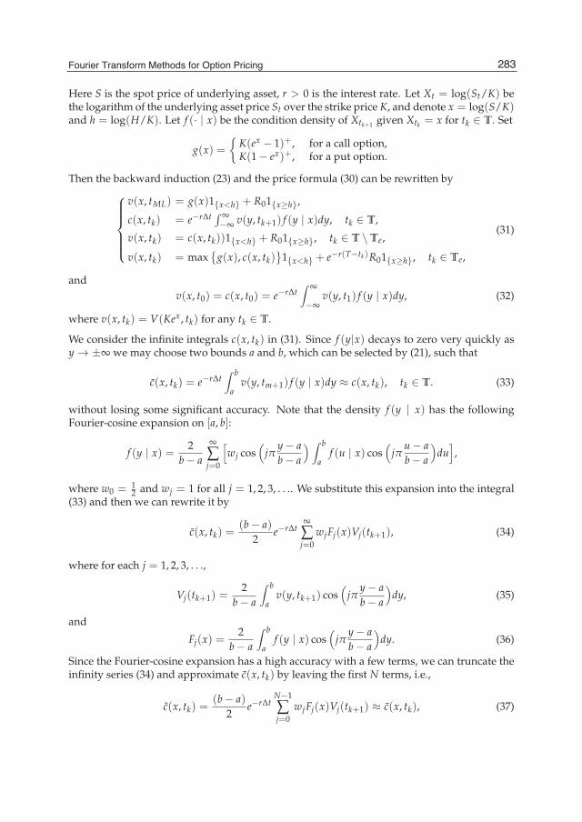
Fourier Transform Methods for Option Pricing 19
Here S is the spot price of underlying asset, r > 0 is the interest rate. Let Xt = log(St/K) bethe logarithm of the underlying asset price St over the strike price K, and denote x = log(S/K)and h = log(H/K). Let f (· | x) be the condition density of Xtk+1 given Xtk = x for tk ∈ T. Set
g(x) ={
K(ex − 1)+, for a call option,K(1 − ex)+, for a put option.
Then the backward induction (23) and the price formula (30) can be rewritten by⎧⎪⎪⎪⎪⎨⎪⎪⎪⎪⎩
v(x, tML) = g(x)1{x<h} + R01{x≥h},
c(x, tk) = e−rΔt ∫ ∞−∞ v(y, tk+1) f (y | x)dy, tk ∈ T,
v(x, tk) = c(x, tk))1{x<h} + R01{x≥h}, tk ∈ T \ Te,
v(x, tk) = max{
g(x), c(x, tk)}
1{x<h} + e−r(T−tk)R01{x≥h}, tk ∈ Te,
(31)
andv(x, t0) = c(x, t0) = e−rΔt
∫ ∞
−∞v(y, t1) f (y | x)dy, (32)
where v(x, tk) = V(Kex, tk) for any tk ∈ T.
We consider the infinite integrals c(x, tk) in (31). Since f (y|x) decays to zero very quickly asy → ±∞ we may choose two bounds a and b, which can be selected by (21), such that
c(x, tk) = e−rΔt∫ b
av(y, tm+1) f (y | x)dy ≈ c(x, tk), tk ∈ T. (33)
without losing some significant accuracy. Note that the density f (y | x) has the followingFourier-cosine expansion on [a, b]:
f (y | x) =2
b − a
∞
∑j=0
[wj cos
(jπ
y − ab − a
) ∫ b
af (u | x) cos
(jπ
u − ab − a
)du
],
where w0 = 12 and wj = 1 for all j = 1, 2, 3, . . .. We substitute this expansion into the integral
(33) and then we can rewrite it by
c(x, tk) =(b − a)
2e−rΔt
∞
∑j=0
wjFj(x)Vj(tk+1), (34)
where for each j = 1, 2, 3, . . .,
Vj(tk+1) =2
b − a
∫ b
av(y, tk+1) cos
(jπ
y − ab − a
)dy, (35)
and
Fj(x) =2
b − a
∫ b
af (y | x) cos
(jπ
y − ab − a
)dy. (36)
Since the Fourier-cosine expansion has a high accuracy with a few terms, we can truncate theinfinity series (34) and approximate c(x, tk) by leaving the first N terms, i.e.,
c(x, tk) =(b − a)
2e−rΔt
N−1
∑j=0
wjFj(x)Vj(tk+1) ≈ c(x, tk), (37)
283Fourier Transform Methods for Option Pricing

20 Will-be-set-by-IN-TECH
for any tk ∈ T, where w0 = wN−1 = 12 and wj = 1 for j = 1, . . . , N−2. On the other hand, we
can represent each integral (36) by approximation as the following
Fj(x) =2
b − aRe
{exp
(− i
jaπ
b − a
) ∫ b
af (u | x) exp
(i
juπ
b − a
)du
}≈ 2
b − aRe
{exp
(− i
jaπ
b − a
) ∫ ∞
−∞f (u | x) exp
(i
jπb − a
u)
du}
.
Let ϕ(u; x) be the characteristic function of f (· | x). Then, we can approximate each Fj(x) by
Fj(x) ≈ 2b − a
Re{
exp(− i
jaπ
b − a
)· ϕ
( jπb − a
; x)}
.
And so, we get the further numerical approximations of the integrals c(x, tk) in (37) by
c(x, tk) = e−rΔtN−1
∑j=0
wjRe{
exp(− i
jaπ
b − a
)· ϕ
( jπb − a
; x)}
Vj(tk+1) ≈ c(x, tj). (38)
In special, the approximation of initial price v(x, t0) in (32) is given by
v(x, t0) = e−rΔtN−1
∑j=0
wjRe{
exp(− i
jaπ
b − a
)· ϕ
( jπb − a
; x)}
Vj(t1). (39)
Meanwhile, since the characteristic function φ(u; x) possesses the property:
ϕ(u; x) = ϕ(u) · eiux, u ∈ R,
where ϕ(u) = ϕ(u; 0), the approximations (38) and (39) can be simplified to
c(x, tk) = e−rΔtN−1
∑j=0
wjRe{
exp(
ijπx − ab − a
)· ϕ
( jπb − a
)}Vj(tk+1), (40)
and the initial price of option
v(x, t0) = e−rΔtN−1
∑j=0
wjRe{
exp(
ijπx − ab − a
)· ϕ
( jπb − a
)}Vj(t1). (41)
In order to use this approximate formulation we still need to compute the integrals Vj(tk). Forconvenience we introduce the following notions: for any a ≤ x1 ≤ x2 ≤ b,
Cj(x1, x2; tk) =2
b − a
∫ x2
x1
c(x, tk) cos(
jπx − ab − a
)dx, j = 0, 1, . . . , N−1,
andDj(x1, x2) =
2R0b − a
∫ x2
x1
cos(
jπx − ab − a
)dx, j = 0, 1, . . . , N−1,
where c(x, tML) = g(x), and c(x, tk), tk ∈ T, are given in (40).
284 Fourier Transform Applications
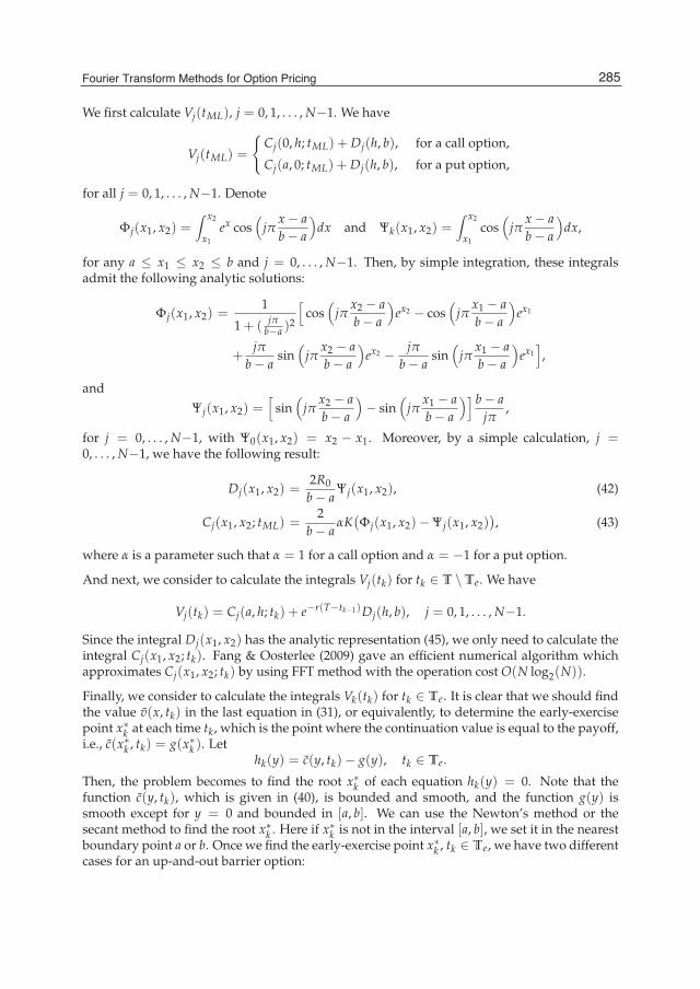
Fourier Transform Methods for Option Pricing 21
We first calculate Vj(tML), j = 0, 1, . . . , N−1. We have
Vj(tML) =
{Cj(0, h; tML) + Dj(h, b), for a call option,
Cj(a, 0; tML) + Dj(h, b), for a put option,
for all j = 0, 1, . . . , N−1. Denote
Φj(x1, x2) =∫ x2
x1
ex cos(
jπx − ab − a
)dx and Ψk(x1, x2) =
∫ x2
x1
cos(
jπx − ab − a
)dx,
for any a ≤ x1 ≤ x2 ≤ b and j = 0, . . . , N−1. Then, by simple integration, these integralsadmit the following analytic solutions:
Φj(x1, x2) =1
1 + (jπ
b−a )2
[cos
(jπ
x2 − ab − a
)ex2 − cos
(jπ
x1 − ab − a
)ex1
+jπ
b − asin
(jπ
x2 − ab − a
)ex2 − jπ
b − asin
(jπ
x1 − ab − a
)ex1
],
andΨj(x1, x2) =
[sin
(jπ
x2 − ab − a
)− sin
(jπ
x1 − ab − a
)] b − ajπ
,
for j = 0, . . . , N−1, with Ψ0(x1, x2) = x2 − x1. Moreover, by a simple calculation, j =0, . . . , N−1, we have the following result:
Dj(x1, x2) =2R0
b − aΨj(x1, x2), (42)
Cj(x1, x2; tML) =2
b − aαK
(Φj(x1, x2)− Ψj(x1, x2)
), (43)
where α is a parameter such that α = 1 for a call option and α = −1 for a put option.
And next, we consider to calculate the integrals Vj(tk) for tk ∈ T \ Te. We have
Vj(tk) = Cj(a, h; tk) + e−r(T−tk−1)Dj(h, b), j = 0, 1, . . . , N−1.
Since the integral Dj(x1, x2) has the analytic representation (45), we only need to calculate theintegral Cj(x1, x2; tk). Fang & Oosterlee (2009) gave an efficient numerical algorithm whichapproximates Cj(x1, x2; tk) by using FFT method with the operation cost O(N log2(N)).
Finally, we consider to calculate the integrals Vk(tk) for tk ∈ Te. It is clear that we should findthe value v(x, tk) in the last equation in (31), or equivalently, to determine the early-exercisepoint x∗k at each time tk, which is the point where the continuation value is equal to the payoff,i.e., c(x∗k , tk) = g(x∗k ). Let
hk(y) = c(y, tk)− g(y), tk ∈ Te.
Then, the problem becomes to find the root x∗k of each equation hk(y) = 0. Note that thefunction c(y, tk), which is given in (40), is bounded and smooth, and the function g(y) issmooth except for y = 0 and bounded in [a, b]. We can use the Newton’s method or thesecant method to find the root x∗k . Here if x∗k is not in the interval [a, b], we set it in the nearestboundary point a or b. Once we find the early-exercise point x∗k , tk ∈ Te, we have two differentcases for an up-and-out barrier option:
285Fourier Transform Methods for Option Pricing

22 Will-be-set-by-IN-TECH
Case 1: x∗k < h, which means the early-exercise point doesn’t hit the up barrier. Thus, We havethe authority to decide to execute the option now or reserve it to the next time point. So wecan split the integral that defines Vj(tk) into three parts: [a, x∗k ], (x∗k , h) and [h, b]. We have
Vj(tk) =
{Cj(a, x∗k ; tk) + Cj(x∗k , h; tML) + e−r(T−tk−1)Dj(h, b), for a call option,
Cj(a, x∗k ; tML) + Cj(x∗k , h; tk) + e−r(T−tk−1)Dj(h, b), for a put option.
Case 2: x∗k ≥ h , which means the early-exercise point hits the up barrier. Thus, the optionintegral can be split into two parts: [a, h) and [h, b]:
Vj(tk) =
{Cj(a, h; tk) + e−r(T−tk−1)Dj(h, b), for a call option,
Cj(a, h; tML) + e−r(T−tk−1)Dj(h, b), for a put option,
Ding et al (2011a) gave a detail algorithm, which summarizes the above procedure, for pricingan up-and-out Bermudan barrier option, and the corresponding numerical experiments.
4.3 The fast Hilbert transform approach for pricing barrier options
Feng & Linetsky (2008) presented a new numerical method to price discretely monitoredbarrier options under exponential Lévy models. Their method involves the relation withHilbert transform (Property P4) and the Sine expansion in Hardy spaces. They also gavean efficient computational algorithm based on the fast Hilbert transform.
Let T = {tk : k = 1, . . . , M} be the set of pre-specified monitored dates, where
0 = t0 < t1 < · · · < tM = T with Δt = tk − tk−1 = T/M.
We consider a European-type barrier put option whose payoff at maturity T is given by
G = 1{St1>L}1{St2>L} · · · 1{StM>L}(K − ST)+,
where K is the strike price and 0 < L < K is the lower barrier. We also assume that theunderlying asset price process is given by St = KeXt with S0 = S, where Xt is a Lévy processstarted at x = log(S/K). Denoting l = log(L/K), then, with help of the risk-neutral valuationformula, the price of this option is given by
V(x, t0) = e−rTE[1{Xt1>l}1{Xt2>l} · · · 1{XtM>l}K(1 − eXtM )+ | X0 = x
],
which can be computed recursively by the following backward induction:⎧⎪⎪⎨⎪⎪⎩
V(x, tM) = 1{x>l}K(1 − ex)+,
V(x, tk) = e−rΔt1{x>l}E[V(Xtk+1 , tk+1) | Xtk = x
], k = M−1, . . . , 1,
V(x, t0) = e−rTE[e−rΔtV(Xt1 , t1) | Xt0 = x
].
(44)
Since each Lévy process is stationary and has independent increments, for each k =1, . . . , M−1, we have
E[V(Xtk+1 , tk+1) | Xtk = x
]= E
[V(Xt1 , tk+1) | Xt0 = x
].
286 Fourier Transform Applications

Fourier Transform Methods for Option Pricing 23
Thus, letting Pt1 v(x) = E[v(Xt1 ) | Xt0 = x
]be the expectation operator, from the backward
induction (44) we get ⎧⎪⎨⎪⎩
vM(x) = 1{x>l} · K(1 − ex)+,
vk(x) = 1{x>l}Pt1 vk+1(x), j = M−1, . . . , 1,
v0(x) = Pt1 v1(x),
(45)
where vk(x) = erΔtV(x, tk). And hence, the problem now becomes to find the function v0(x)from the backward induction (45).
Note that 1{x>0} = 12(1 + sgn(x)
)for all x ∈ R. Using the Property P4 (Relation with Hilbert
transform) we obtain
F (1{x>0} · v)(u) =12(Fv(u) + iH(Fv)(u)
). (46)
Let a ∈ R and Ta be the transform operator: Tav(x) = v(x − a). Then, we have
1{x>a} = Ta1{x>0} =12(1 + Tasgn(x)
),
and hence,
1{x>a} · v(x) =12(v(x) + v(x) · Tasgn(x)
)=
12
(v(x) + Ta
(sgn · T−av
)(x)
).
Taking the Fourier transform to both sides of this equation, we have
F(1{x>a} · v
)(u) =
12Fv(u) +
12F(Ta
(sgn · T−av
))(u).
and using equation (46) we obtain
F(1{x>a} · v
)(u) =
12Fv(u) +
12
ieiauH(e−iayFv(y)
)(u). (47)
On other hand, noting that, for each k = 1, . . . , M−1, the condition density of Xtk+1 givenXtk = x possesses the property:
f (y|x) = f (y−x), x, y ∈ R,
where f (y) is the density of Xt1 under the initial condition Xt0 = x. The infinite integralsPt1 vk+1(x) in (45) becomes to
Pt1 vk+1(x) =∫ +∞
−∞vk+1(y) f (y−x)dy =
∫ +∞
−∞vk+1(x+z) f (z)dz.
Then, this integral can be rewritten as a convolution of vk+1(x+z) and the function f (−x), i.e.
Pt1 vk+1(x) = f (−x) ∗ vk+1(x).
Note that suppvk(x) ⊂ (l, 0) for each k = M, . . . , 1 from the backward induction (45). We cantake the Fourier transform in the both sides of (45). Applying the Property P3 (Convolution)we have
F [Pt1 vk(x)
](u) = F [
f (−x) ∗ vk+1(x)](u) = F [
f (−x)](u) · F [
vk+1(x)](u).
287Fourier Transform Methods for Option Pricing

24 Will-be-set-by-IN-TECH
Denote ϕ(u) is the characteristic function of f (x) on the complex plane C. Then, by a simplecalculation, we have
F [Pt1 vk(x)
](u) = ϕ(−u) · Fvk+1(u). (48)
Thus, using the formulas (47) and (48) we obtain⎧⎪⎪⎪⎪⎨⎪⎪⎪⎪⎩
vM(u) = K(1−eiul)iu − K(1−e(1+iu)l)
1+iu ,
vk(u) = 12 ϕ(−u)vk+1(u) + 1
2 ieiulH(e−iyl ϕ(−y)vk+1(y)
)(u),
k = M−1, . . . , 1,v0(u) = ϕ(−u)v1(u).
(49)
Here vk(u) = Fvk(u) for each k. Applying the truncated Sinc approximation, Feng & Linetsky(2008) obtained the discretization of vk(u):
vk(nh) =12
ϕ(−nh)vk+1(nh)
+ieinhl
2π
N
∑j=−N,j �=n
e−ijhl ϕ(−jh)vk+1(jh)1 − (−1)n−j
n − j, (50)
for n = −N, . . . , N and k = M−1, . . . , 1, where N is a positive integer and h is thediscretization step size. Then, the function v0(x) can be computed by the discretised inversionFourier transform:
v0(x) =1
2π
N
∑j=−N
e−ijhx ϕ(−jh)v1(jh)h.
Furthermore, Feng & Linetsky (2008) showed that the computation (50) involves a Toeplitzmatrix-vector multiplication, which can be accomplished in O(N log2 N) operations using theFFT technique. They also referred the corresponding algorithm of computing the discreteHilbert transform via the FFT as the Fast Hilbert Transform.
5. References
Barndorff-Nielsen, O. (1997). Normal inverse Gaussian distributions and stochastic volatilitymodelling, Scandinavian Journal of Statistics, Vol. 24, pp. 1–13.
Bates, D. S. (1996). Jumps and stochastic volatility: exchange rate processes implicit inDeutsche mark options, Rev. Financ. Stud., Vol. 9, pp. 69–107.
Black, F. & Scholes, M. (1973). The pricing of options and corporate liabilities, Journal of PoliticalEconomy, Vol. 81 (No. 3), pp. 637–654.
Borak, S., Detlefsen, K. & Härdle, W. (2005). FFT based option pricing, SFB 649 Discussionpaper 2005-011. http://sfb649.wiwi.hu-berlin.de
Carr, P., Geman, H., Madan, D. & Yor, M. (2002). The fine structure of asset returns: Anempirical investigation. Journal of Business, Vol. 75, pp. 305–332.
Carr, P. & Madan, D. (1999). Option valuation using the fast Fourier transform, Journal ofComputational Finance, Vol. 2 pp. 61–73.
Carr, P. & Wu, L. (2003). The finite moment log stable process and option pricing, Journal ofFinance, Vol. 58, pp. 753–777.
Cont, R. & Tankov, P. (2003). Financial Modelling with Jump Processes, Chapman & Hall/ CRCPress.
288 Fourier Transform Applications

Fourier Transform Methods for Option Pricing 25
Dempster, M. A. & Hong, S. S. G. (2002). Spread option valuation and the fast Fouriertransform, Mathematical Finance–Bachelier Congress 2000, Spring, pp. 203–220.
Ding, D & U, S. C. (2010). An accurate and stable FFT-based method for pricing options underexp-Levy processes, The Proceedings of ISCM II - EPMSC XII, American Institute ofPhysics, pp. 741–746.
Ding, D & U, S. C. (2011). Efficient option pricing methods based on Fourier series expansions,Journal of Mathematical Research and Exposition, Vol. 31, pp. 12–22.
Ding, D., Huang, H. & Zhao, J. (2011a). An efficient algorithm for Bermudan barrier optionpricing, Working paper, University of Macau.
Ding, D., Weng, Z. & Zhao, J. (2011b). Pricing Bermudan barrier options via a fast and accurateFFT-based Method, to appear in the Proceedings of CiSE 2011, IEEE.
Duffie, D., Pan, J. & Singleton, K. (2000). Transform analysis and asset pricing for affinejump-diffusions, Econometrica, Vol. 68, pp. 1343–1376.
Dufresne, D., Garrido, J. & Morales, M. (2009). Fourier inversion formulas in option pricingand insurance, Methodol. Comput. Appl. Probab., Vol. 11, pp. 359–383.
Eberlein, E., Glau, K., & Papapantoleon, A. (2010). Analysis of Fourier transform valuationformulas and application, Applied Mathematical Finance, Vol. 17, pp. 211–240.
Fang, F. & Oosterlee, C. W. (2008). A novel pricing method for European option based onFourier-cosine series expansions, SIAM J. Sci. Comput., Vol. 31, pp. 826–848.
Fang, F. & Oosterlee, C. W. (2009). Pricing early-exercise and discrete barrier options byFourier-cosine series expansions, Numer. Math., Vol. 114, pp. 27–62.
Fang, F. & Oosterlee, C. W. (2011). A Fourier-based valuation method for Bermudan andbarrier options under Heston’s model, SIAM J. Financial Math., Vol. 2, pp. 439–463.
Feng, L. & Linetsky, V. (2008). Pricing discretely monitored barrier options and defaultablebonds in Lévy process models: a fast Hilbert transform approach. MathematicalFinance, Vol. 18, pp. 337–384.
Gurland, J. (1948). Inversion formula for the distribution of ratios, Ann. Math. Statist., Vol. 19,pp. 228–237.
Heston, S. (1993). A closed-form solution for options with stochastic volatility withapplications to bond and currency options, Rev. Financ. Stud., Vol. 6, pp. 327–343.
Hurd, T. & Zhou, Z. (2010). A Fourier transform method for spread option pricing, SIAM J.Finan. Math., Vol. 1, pp. 142–157.
Lee, R. (2004). Option pricing by transform methods: Extensions, unification, and errorcontrol, Journal of Computational Finance, Vol. 7, pp. 51–86.
Lewis, A. (2001). A simple option formula for general jump-diffusion and other exponentialLévy processes. http://www.optioncity.net
Lord, R., Fang, F., Bervoets, F. & Oosterlee, C. W. (2008). A fast and accurate FFT-based methodfor pricing early-exercise options under Lévy processes. SIAM J. Sci. Comput., Vol. 30,pp. 1678–1705.
Kou, S. G. (2002). A jump-diffusion model for option pricing, Management Science, Vol. 48, pp.1086-1101.
Kwok, Y. K., Leung, K. S. & Wong, H. Y. (2010). Efficient options pricing using the fast Fouriertransform. http://ssrn.com/abstract=1534544
Madan, D., Carr, P. & Chang, E. (1998). The variance gamma process and option pricing,European Financial Review, Vol. 2, pp. 79–105.
Merton, R. (1973). Theory of rational option pricing, Bell Journal of Economics and ManagementScience , Vol. 4, pp. 141–183.
289Fourier Transform Methods for Option Pricing

26 Will-be-set-by-IN-TECH
Merton, R. (1976). Option pricing when underlying stock returns are discontinuous. J. Financ.Econ., Vol. 3, pp. 125–144.
Schmelzle, M. (2010). Option Pricing Formulae using Fourier Transform: Theoryand Application. http://pfadintegral.com/articles/option-pricing-formulae-using-fourier-transform/
Shephard, N. G. (1991). From characteristic function to distribution function: a simpleframework for the theory, Econometric Theory, Vol. 7, pp. 519–529.
Stein, E. & Stein, F. (1991). Stock price distribution with stochastic volatility: An analyticapproach, Rev. Financ. Stud., Vol. 4, pp. 727–752.
290 Fourier Transform Applications

0
Hilbert Transform and ApplicationsYi-Wen Liu
National Tsing Hua UniversityTaiwan
1. Introduction
Hilbert transform finds a companion function y(t) for a real function x(t) so that z(t) = x(t) +iy(t) can be analytically extended from the real line t ∈ R to upper half of the complex plane.
In the field of signal processing, Hilbert transform can be computed in a few steps:First, calculate the Fourier transform of the given signal x(t). Second, reject the negativefrequencies. Finally, calculate the inverse Fourier transform, and the result will be acomplex-valued signal where the real and the imaginary parts form a Hilbert-transform pair.
When x(t) is narrow-banded, |z(t)| can be regarded as a slow-varying envelope of x(t)while the phase derivative ∂t[tan−1(y/x)] is an instantaneous frequency. Thus, Hilberttransform can be interpreted as a way to represent a narrow-band signal in terms of amplitudeand frequency modulation. The transform is therefore useful for diverse purposes such aslatency analysis in neuro-physiological signals (Recio-Spinoso et al., 2011; van Drongelen,2007), design of bizarre stimuli for psychoacoustic experiments (Smith et al., 2002), speechdata compression for communication (Potamianos & Maragos, 1994), regularization ofconvergence problems in multi-channel acoustic echo cancellation (Liu & Smith, 2002), andsignal processing for auditory prostheses (Nie et al., 2006).
The rest of this review chapter is organized as follows: Sec. 2 reviews the mathematicaldefinition of Hilbert transform and various ways to calculate it. Secs. 3 and 4 reviewapplications of Hilbert transform in two major areas: Signal processing and systemidentification. The chapter concludes with remarks on the historical development of Hilberttransform in Sec. 6.
2. Mathematical foundations of Hilbert transform
The desire to construct the Hilbert transform stemmed from this simple quest: Given areal-valued function f : R → R, can we find an imaginary part ig such that fc = f + igcan be analytically extended? For example, if f (x) = cos(x), then by inspection we can findg(x) = sin(x) such that fc(x) = f + ig = exp(ix). This function can obviously be extendedanalytically to the entire complex plane by replacing the real variable x with the complexvariable z in the expression; the result is fext(z) = exp(iz) and we have
Re{ fext(z)}|z=x = f (x), (1)
12

2 Will-be-set-by-IN-TECH
which states that real part of the extended function is equal to the original given function f (x)on the real line. The companion function g(x) is called the Hilbert transform of f (x).
This simple example brings forth a few questions. First, is analytic extension always possiblefor reasonably smooth f (x)? If so, is the companion function g(x) unique, in the sense thatEq. (1) would hold? The answer to the second question is a definite ‘No’, because any fc(x) =f (x) + i{g(x) + g0} also satisfies Eq. (1), where g0 is an arbitrary constant. Therefore, theoriginal simple quest needs to be refined as follows.
2.1 Hilbert transform as a boundary-value problem
To establish the uniqueness of the companion function, we first note that any analyticfunction fext(z) = fR(z) + i f I(z) defined on the complex plane z = x + iy must satisfyCauchy-Riemann equations,
∂ fR∂x
=∂ f I∂y
,
∂ f I∂x
= − ∂ fR∂y
.
Consequently, both fR and f I satisfy Laplace’s equation,
∂2FR∂x2 +
∂2FR∂y2 = 0, (2)
∂2FI∂x2 +
∂2FI∂y2 = 0 (3)
over the region where fext(z) is analytic. Conventionally, by requiring fext(z) to be analytic inthe upper half-plane, the quest of finding the Hilbert transform for any given function f (x)can be formulated as a boundary value problem (Scott, 1970). By specifying the boundaryconditions that
• fR(x, 0) = f (x), and that• fR(x, y) = 0 as x → ±∞ or y → ∞,
fR(x, y) can be uniquely determined by solving Laplace’s equation (Eq. 2) in the upper halfplane. Then, through Cauchy-Riemann equations, f I(x, y) can be calculated in the entireupper half plane and in particular on its boundary the x-axis (Scott, 1970). Thus g(x) =FI(x, 0) is the Hilbert transform of the given function f (x).
2.2 Calculation through improper integrals
The above formulation of Hilbert transform as a boundary-value problem is hardly mentionedin recent texts [except as an exercise problem in Oppenheim & Schafer (2010)].1: Instead,
1 The boundary-value-problem formulation is missing for a reason — it does not tell us how to computethe Hilbert transform.
292 Fourier Transform Applications
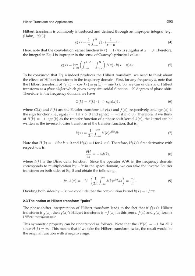
Hilbert Transform and Applications 3
Hilbert transform is commonly introduced and defined through an improper integral [e.g.,(Hahn, 1996)]:
g(x) =1π
∫ ∞
−∞f (u)
1x − u
du. (4)
Here, note that the convolution kernel function h(x) = 1/πx is singular at x = 0. Therefore,the integral in Eq. 4 is improper in the sense of Cauchy’s principal value:
g(x) = limε→0
(∫ x−ε
−∞+
∫ ∞
x+ε
)f (u) · h(x − u)du. (5)
To be convinced that Eq. 4 indeed produces the Hilbert transform, we need to think aboutthe effects of Hilbert transform in the frequency domain. First, for any frequency k, note thatthe Hilbert transform of fk(x) = cos(kx) is gk(x) = sin(kx). So, we can understand Hilberttransform as a phase shifter which gives every sinusoidal function −90 degrees of phase shift.Therefore, in the frequency domain, we have
G(k) = F(k) · (−i · sgn(k)) , (6)
where G(k) and F(k) are the Fourier transform of g(x) and f (x), respectively, and sgn(x) isthe sign function (i.e., sgn(k) = 1 if k > 0 and sgn(k) = −1 if k < 0.) Therefore, if we thinkof H(k) = −i · sgn(k) as the transfer function of a phase-shift kernel h(x), the kernel can bewritten as the inverse Fourier transform of the transfer function; that is,
h(x) =1
2π
∫ ∞
−∞H(k)eikxdk. (7)
Note that H(k) = −i for k > 0 and H(k) = i for k < 0. Therefore, H(k)’s first derivative withrespect to k is
∂H∂k
= −2iδ(k), (8)
where δ(k) is the Dirac delta function. Since the operator ∂/∂k in the frequency domaincorresponds to multiplication by −ix in the space domain, we can take the inverse Fouriertransform on both sides of Eq. 8 and obtain the following,
− ix · h(x) = −2i ·(
12π
∫ ∞
−∞δ(k)eikxdk
)=
−iπ
. (9)
Dividing both sides by −ix, we conclude that the convolution kernel h(x) = 1/πx.
2.3 The notion of Hilbert transform “pairs”
The phase-shifter interpretation of Hilbert transform leads to the fact that if f (x)’s Hilberttransform is g(x), then g(x)’s Hilbert transform is − f (x); in this sense, f (x) and g(x) form aHilbert transform pair.
This symmetric property can be understood as follows. Note that the H2(k) = −1 for all ksince H(k) = ±i. This means that if we take the Hilbert transform twice, the result would bethe original function with a negative sign.
293Hilbert Transform and Applications
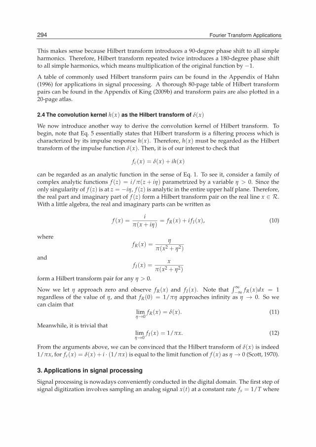
4 Will-be-set-by-IN-TECH
This makes sense because Hilbert transform introduces a 90-degree phase shift to all simpleharmonics. Therefore, Hilbert transform repeated twice introduces a 180-degree phase shiftto all simple harmonics, which means multiplication of the original function by −1.
A table of commonly used Hilbert transform pairs can be found in the Appendix of Hahn(1996) for applications in signal processing. A thorough 80-page table of Hilbert transformpairs can be found in the Appendix of King (2009b) and transform pairs are also plotted in a20-page atlas.
2.4 The convolution kernel h(x) as the Hilbert transform of δ(x)
We now introduce another way to derive the convolution kernel of Hilbert transform. Tobegin, note that Eq. 5 essentially states that Hilbert transform is a filtering process which ischaracterized by its impulse response h(x). Therefore, h(x) must be regarded as the Hilberttransform of the impulse function δ(x). Then, it is of our interest to check that
fc(x) = δ(x) + ih(x)
can be regarded as an analytic function in the sense of Eq. 1. To see it, consider a family ofcomplex analytic functions f (z) = i/π(z + iη) parametrized by a variable η > 0. Since theonly singularity of f (z) is at z = −iη, f (z) is analytic in the entire upper half plane. Therefore,the real part and imaginary part of f (z) form a Hilbert transform pair on the real line x ∈ R.With a little algebra, the real and imaginary parts can be written as
f (x) =i
π(x + iη)= fR(x) + i f I(x), (10)
wherefR(x) =
η
π(x2 + η2)
andf I(x) =
xπ(x2 + η2)
form a Hilbert transform pair for any η > 0.
Now we let η approach zero and observe fR(x) and f I(x). Note that∫ ∞−∞ fR(x)dx = 1
regardless of the value of η, and that fR(0) = 1/πη approaches infinity as η → 0. So wecan claim that
limη→0
fR(x) = δ(x). (11)
Meanwhile, it is trivial thatlimη→0
f I(x) = 1/πx. (12)
From the arguments above, we can be convinced that the Hilbert transform of δ(x) is indeed1/πx, for fc(x) = δ(x) + i · (1/πx) is equal to the limit function of f (x) as η → 0 (Scott, 1970).
3. Applications in signal processing
Signal processing is nowadays conveniently conducted in the digital domain. The first step ofsignal digitization involves sampling an analog signal x(t) at a constant rate fs = 1/T where
294 Fourier Transform Applications

Hilbert Transform and Applications 5
T is the sampling period. In this section, we denote the sampled waveform as x[n] = x(nT),using the square brackets [·] to indicate that the signal is sampled in discrete time. So thediscrete-time Fourier transform (DTFT) is defined as follows:2
X(jω) =∞
∑n=−∞
x[n]e−jωn.
Note that X(jω) is periodic at every 2π in the frequency domain.3 Next, we show how Hilberttransform can be defined in discrete time.
3.1 The discrete-time Hilbert transform and Hilbert transformers
Recall that the Hilbert transform introduce a 90-degree phase shift to all sinusoidalcomponents. In the discrete-time periodic-frequency domain, the transfer function of Hilberttransform is specified as follows,
H(jω) =
{−j, 0 < ω < π
j, −π < ω < 0(13)
The convolution kernel for H(jω) can be calculated through inverse Fourier transform(Oppenheim & Schafer, 2010):
h[n] =1
2π
∫ π
−πH(jω)ejωndω (14)
=
{2π
sin2(πn)n , n �= 0
0, n = 0(15)
Note that h[n] has a infinite support from n = −∞ to ∞. In practice, the entire function cannot be stored digitally. To circumvent this difficulty, we now discuss two major methods forcalculating the discrete-time Hilbert transform.
3.1.1 The MATLAB approach
The universally popular scientific-computing software MATLAB (MathWorks, Natick,Massachusetts, USA) has a hilbert() function that “computes the so-called discrete-timeanalytic signal X = Xr + i*Xi such that Xi is the Hilbert transform of Xr”.4 MATLAB’simplementation of the hilbert() function takes advantage of the fast Fourier transform(FFT). Essentially, the hilbert() function completes the calculation in three steps:
• Do the FFT of Xr.• Set the elements in FFT which correspond to frequency −π < ω < 0 to zero.• Do the inverse FFT.
2 We now switch to the electrical-engineering convention of using j to refer to√−1.
3 Hereafter, we use capital letters X, Y, Z, H, ... to denote spectrums in the frequency domain, andlowercase letters x, y, z, h for signals in the time domain.
4 This is what MATLAB’s help file shows.
295Hilbert Transform and Applications
6 Will-be-set-by-IN-TECH
That the three steps above can work is a consequence of the fact that, if xi[n] is the discreteHilbert transform of xr[n], the Fourier transform of xr[n] + jxi[n] vanishes for all negativefrequencies −π < ω < 0. This can be verified by inspecting the definition given in Eq. 13.
Remarks: Perhaps because of MATLAB’s popularity and easiness to use, many have allegedlymis-regard the returned vector X=hilbert(Xr) as the Hilbert transform of Xr. One must beaware of these deviations from the conventional definition to avoid unnecessary confusion.
3.1.2 Hilbert transform as a filter design problem
Thanks to FFT, MATLAB’s implementation of Hilbert transform is very efficient. However,it should be used with caution — note that the Hilbert transform defined in Eq. 13 has adiscontinuity at ω = 0. Consequently (due to Gibb’s phenomenon), the convolution kernelh[n] in Eq. 15 has an infinite support in time. As a result, when implemented through FFT, theHilbert transform kernel wraps around itself and time-domain aliasing comes in (Oppenheim& Schafer, 2010). The time-domain aliasing could be perceived as artifacts in applications suchas audio and video signal processing.
To avoid time-domain aliasing, one can formulate discrete Hilbert transform as a filter-designproblem. The ideal transfer function is specified by Eq. 13, and there are standard techniquesto design finite impulse response (FIR) or infinite impulse response (IIR) filters that appraochthe ideal transfer function. For example, one can truncate the ideal impulse response bymultiplying it with a window function w[n] which has a finite support (let’s say from n = −Nto N). Then the resulting function w[n]h[n] yields an approximate magnitude responseHw(jω) that has a smooth transition between negative and positive frequencies as well asripples in both regions. The height of the ripples can be reduced by selecting the windowfunction wisely, while the transition bandwidth is inversely proportional to the windowlength. Interested readers can refer to Chapter 7 and 12 of Oppenheim & Schafer (2010).
The FIR or IIR filters designed to approximate Hilbert transform are called Hilbert transformers.Next, we discuss applications of Hilbert transformers in communication and in biomedicalengineering.
3.2 Sampling of bandpass signals for communication
An important application of Hilbert transformers is in sampling bandpass signals.5 To explainthis, let us assume that a bandpass signal s(t) is has a region of support fc ≤ f ≤ fc + Δ f inthe frequency domain, where Δ f = 0.2 fc. Based on Nyquist’s theorem, the sampling rateneeds to be at least two times the highest frequency, or 2.4 fc, to avoid frequency-domainaliasing. However, the bandwidth of this signal is really Δ f = 0.2 fc, so fs = 2.4 fc is in fact anoversampling.
To take advantage of the narrow bandwidth, we initially need to sample at 2.4 fc to obtainedan oversampled signal sr[n] = s(nT), where T = 1/ fs. Then, we can use a Hilbert transformerto obtain si[n] such that the Fourier transform of s[n] = sr[n] + jsi[n] has no components atnegative frequencies π < ω < 0. Now, S(jω)’s region of support is ω ∈ (5π/6, π). Therefore,we can down sample s[n] by a factor of 6 and there would be no frequency-domain aliasing.
5 This part is adapted from Sec. 12.4.3 of Oppenheim & Schafer (2010)
296 Fourier Transform Applications

Hilbert Transform and Applications 7
Transmitting sd[n] = s[6n] is more efficient than transmitting sr[n] because the sampling rateis lowered.
To reconstruct sr[n] from sd[n], we can do the following:
• Expand sd[n] by a factor of 6; i.e., construct se[n] =
{sd[n/6], if n = 0,±6,±12, ...0, otherwise.
• Filter se[n] with the passband of (5π/6, π).• Take the real part, and the result is a reconstructed copy of sr[n].
In practice, since all Hilbert bandpass filters are not ideal, one needs to consider samplingat slightly higher than 2.4 fc. That would protect the passband from ripple interference bothduring downsampling and during signal reconstruction.
3.3 AM-FM decomposition for auditory prostheses
A cochlear implant device consists of up to tens of electrodes which are inserted as an array tothe cochlea to stimulate auditory nerves by electrical currents (Zeng et al., 2008). Each channel(electrode) represents an acoustic frequency band; the amount of currents sent to an electrodeshould faithfully reflect how acoustic energy entering through the ear microphone varies intime in the corresponding frequency band. Typically, acoustic waveforms are processed witha bank of filters and the resulting envelopes control the electrical currents sent to individualelectrodes.
In this application scenario, a Hilbert transformer has been found useful for envelopeextraction. This can be understood by noting that the Hilbert transform produces a sin(ωt) forevery cos(ωt). For a narrow-band signal sR(t), we can factor it as a product of slow-varyingenvelope A(t) and fast-varying fine structure f (t):
sR(t) = A(t) f (t) = A(t) cos[φ(t)]
where dφ(t)/dt can be regarded as an instantaneous frequency of the signal. It can be shownthat, if A(t) varies sufficiently slowly, the Hilbert transform produces approximately sI(t) =A(t) sin[φ(t)]. Then, the envelope A(t) can simply be estimated by taking the root of sum ofsquares:
A(t) �√
s2R(t) + s2
I (t). (16)
Clinically, encoding the currents based on A(t) provides clear speech perception forcochlear-implant users (Nie et al., 2006). Moreover, auditory pitch information can beextracted by taking the time-derivation of φ(t), which can be determined by the relative phasebetween sI and sR:
φ(t) = tan−1(
sI(t)sR(t)
).
Pitch is arguably the utmost important feature for music perception as well as understandingtonal languages. Here, we see Hilbert transform can serve as an efficient computation tool toextract it.
297Hilbert Transform and Applications
8 Will-be-set-by-IN-TECH
4. Applications in system identification
Hilbert transform relates the real part and the imaginary part of the transfer function ofany physically viable linear time-invariant system. By “physical viability” we mean a systemshould be stable and causal. Stability requires the systems to produce bounded output ifthe input is bounded [so called the bounded-input bounded-output criterion, (Oppenheim &Schafer, 2010)]. Causality prohibits the system from producing responses before any stimuluscomes in. Denote the impulse response as h(t) and its Laplace transform as H(s). The aboveconditions requires that
• h(t) = 0 for all t < 0 (causality)• All sigularities of H(s) are located in the left half-plane (stability).
The two conditions above ensure that H(s) converges and is analytic in the entire righthalf-plane, and in particular on the imaginary axis s = jω. Therefore, the real and imaginarypart of H(jω) = HR(ω) + jHI(ω) are inter-dependent in term of the Kramers-Krönig relations(King, 2009b):
HI(ω) =1π
∫ ∞
−∞
HR(u)duω − u
(17)
HR(ω) = − 1π
∫ ∞
−∞
HI(u)duω − u
(18)
which is basically Hilbert transform in its time-frequency dual form.
The Kramers-Krönig relations govern how physical viable transfer functions can vary infrequency. For instance, the real and imaginary part of an electromagnetic wave propagationfunction defines the attenuation and the wavenumber per unit length as a function offrequency. The frequency dependence of both functions is referred to as dispersion, for in opticsit describes how red light travels faster than violet light in water — so we behold the beautyof rainbows after raining. It is now intriguing to realize that the attenuation and velocity oflight are two inter-dependent functions of frequency. More physics-inclined readers can referto King’s thorough discussion on dispersion relations in electrodynamics and optics (King,2009b).
To a certain extent, the concept that the real and the imaginary parts are inter-dependentsimilarly applies to the magnitude and phase of transfer functions of a physically viablesystem. Note that any transfer function H(jω) can be decomposed logarithmically intomagnitude and phase:
log H(jω) = log |H(jω)|+ j∠H(jω).
This shows that the log-magnitude and the phase are real and imaginary parts of thelog-spectrum, respectively. It might appear that they must satisfy the Kramers-Krönigrelations. Unfortunately, this is a wishful thinking since apparently H(jω) =exp(−jωτ)H(jω), where τ is a constant, would have the same magnitude as H(jω) but adifferent phase response.6
It turns out that, for any given magnitude response, the uniqueness of phase response can beestablished if the transfer function satisfies a minimum-phase criterion; the criterion requires
6 in fact, h(t) = h(t − τ).
298 Fourier Transform Applications

Hilbert Transform and Applications 9
that all zeros and poles of the transfer function H(s) to be located in the left-half plane. Thiscriterion ensures that all the singularities of log H(s) are located in the left-half plane so thereal and imaginary parts of log H(s) become a Hilbert transform pair. Otherwise, any transferfunction can be uniquely factorized as a product of a minimum-phase function M(jω) andan all-pass function P(jω). It is noteworthy that the system whose transfer function is M(jω)has the minimal energy delay among all linear time-invariant systems of the same magnituderesponse. Further readings are recommended in Chapter 5 and 12 of Oppenheim & Schafer(2010).
5. Concluding remarks and historical developments
In this chapter, we first presented Hilbert transform as an analytic extension problem. Hilberttransform uniquely exists due to Cauchy-Riemann equations. We then reviewed severaldifferent ways to calculate Hilbert transform. A few important points stand out: First, Hilberttransform can be regarded as a 90-degree phase shifter. Secondly, the real part and imaginarypart of a physically viable transfer function must satisfy Kramers-Krönig relations, which isthe Hilbert transform applied in time-frequency duality. A good reference on these topics canbe found in Oppenheim & Schafer (2010).
The construction of Hilbert transform pairs through Cauchy-Riemann equations in Sec. 2.1was found in the appendices of an old text on microwave electronics (Scott, 1970). Theoriginal formulation was stated in terms of Kramers-Krönig relation, and in this chapter thatformulation is adapted so the signal is defined on the real line instead of the frequency axisjω.
As a matter of fact, the definition of Hilbert transform was not given by David Hilbert himself.The name “Hilbert transform” was first given by the British mathematician G. H. Hardy inhonor of Hilbert’s pioneering work on integral equations (King, 2009a). Hardy’s early workestablished mathematical rigor of the transform (Hardy, 1932), which we now apply in variousareas such as physiology and telecommnication. A review of these contributions from brilliantmathematicians reminds us that the transform really is a heritage from the 20th century.Nevertheless, it is also amusing that nowadays we calculate Hilbert transform with superfast computers, which might never had been envisioned by 20th-century pioneers, includingHilbert, Hardy, Scott, or even Oppenheim.
6. Acknowledgement
This work is supported by Taiwan’s National Science Council through research grantNo. 100-2221-E-007-011.
7. References
Hahn, S. L. (1996). Hilbert Transforms in Signal Processing, Artech House, Inc., Norwood, MA,USA.
Hardy, G. H. (1932). On hilbert transforms, Quart. J. Math. (Oxford) 3: 102–112.King, F. W. (2009a). Hilbert Transforms, Vol. 1, Cambridge University Press, Cambridge, UK.King, F. W. (2009b). Hilbert Transforms, Vol. 2, Cambridge University Press, Cambridge, UK.
299Hilbert Transform and Applications

10 Will-be-set-by-IN-TECH
Liu, Y.-W. & Smith, J. O. (2002). Perceptually similar orthogonal sounds and applications tomultichannel acoustic echo canceling, Proc. Audio Eng. Soc. 22nd Int. Conf., Espoo,Finland.
Nie, K., Barco, A. & Zeng, F.-G. (2006). Spectral and temporal cues in cochlear implant speechperception, Ear Hear. 27: 208–217.
Oppenheim, A. V. & Schafer, R. W. (2010). Discrete-Time Signal Processing, 3rd Edition, Pearson,Boston.
Potamianos, A. & Maragos, P. (1994). A comparison of the energy operator and the hilberttransform approach to signal and speech demodulation, Signal Processing 37(1): 95 –120.
Recio-Spinoso, A., Fan, Y.-H. & Ruggero, M. (2011). Basilar-membrane responses tobroadband noise modeled using linear filters with rational transfer functions,Biomedical Engineering, IEEE Transactions on 58(5): 1456 –1465.
Scott, A. (1970). Active and Nonlinear Wave Propagation in Electronics, Wiley-Interscience, NewYork.
Smith, Z. M., Delgutte, B. & Oxenham, A. J. (2002). Chimaeric sounds reveal dichotomies inauditory perception, Nature 416: 87–90.
van Drongelen, W. (2007). Signal Processing for Neuroscientists: Introduction to the analysis ofphysiological signals, Academic Press, London.
Zeng, F.-G., Rebscher, S., Harrison, W., Sun, X. & Feng, H. (2008). Cochlear implants: Systemdesign, integration, and evaluation, IEEE Rev. Biomed. Eng. 1: 115–142.
300 Fourier Transform Applications