fourier series { complex form
TRANSCRIPT

6.003: Signal Processing
Fourier Series – Complex Form
• complex numbers, complex exponentials, and their relation to sinusoids
• complex exponential form of Fourier series
• properties of Fourier series
February 11, 2020

Last Week
Representing a signal as a Fourier series.
Synthesis Equation
f(t) = c0 +∞∑k=1
ck cos(kωot) +∞∑k=1
dk sin(kωot) where ωo = 2πT
Analysis Equations
c0 = 1T
∫Tf(t) dt
ck = 2T
∫Tf(t) cos(kωot) dt
dk = 2T
∫Tf(t) sin(kωot) dt
Today: Simplifying the math with complex numbers.

Simplifying Math By Using Complex Numbers
Complex numbers simplify thinking about roots of numbers / polynomials:
• all numbers have two square roots, three cube roots, etc.
• all polynomials of order n have n roots (but some may be repeated).
Our biggest simplification comes from Euler’s formula, which relates com-
plex exponentials to trigonometric functions (Leonhard Euler, 1748).
ejθ = cos θ + j sin θwhere j =
√−1.
Richard Feynman called this ”the most remarkable formula in mathemat-
ics.”
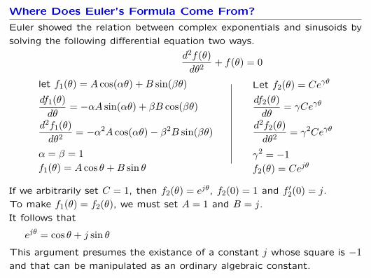
Where Does Euler’s Formula Come From?
Euler showed the relation between complex exponentials and sinusoids by
solving the following differential equation two ways.
d2f(θ)dθ2 + f(θ) = 0
let f1(θ) = A cos(αθ) +B sin(βθ)df1(θ)dθ
= −αA sin(αθ) + βB cos(βθ)
d2f1(θ)dθ2 = −α2A cos(αθ)− β2B sin(βθ)
α = β = 1f1(θ) = A cos θ +B sin θ
Let f2(θ) = Ceγθ
df2(θ)dθ
= γCeγθ
d2f2(θ)dθ2 = γ2Ceγθ
γ2 = −1f2(θ) = Cejθ
If we arbitrarily set C = 1, then f2(θ) = ejθ, f2(0) = 1 and f ′2(0) = j.
To make f1(θ) = f2(θ), we must set A = 1 and B = j.
It follows that
ejθ = cos θ + j sin θThis argument presumes the existance of a constant j whose square is −1and that can be manipulated as an ordinary algebraic constant.

Where Does Euler’s Formula Come From?
Euler’s formula also follows from Maclaurin expansion of the exponential
function, assuming the j behaves like any other algebraic constant.
Start with the expansion of the real-valued function:
eθ = 1 + θ + θ2
2! + θ3
3! + θ4
4! + θ5
5! + θ6
6! + θ7
7! + · · ·
Assume that the same expansion holds for complex-valued arguments:
ejθ = 1 + jθ + j2θ2
2! + j3θ3
3! + j4θ4
4! + j5θ5
5! + j6θ6
6! + j7θ7
7! + · · ·
= 1 + jθ − θ2
2! −jθ3
3! + θ4
4! + jθ5
5! −θ6
6! −jθ7
7! + · · ·
=(
1− θ2
2! + θ4
4! −θ6
6! + · · ·)
︸ ︷︷ ︸cos θ
+j(θ − θ3
3! + θ5
5! −θ7
7! + · · ·)
︸ ︷︷ ︸sin θ
Euler’s formula results by splitting the even and odd powers of θ.
ejθ = cos θ + j sin θ

Geometric Interpretation
In 1897, Caspar Wessel was the first to describe complex numbers as points
in the complex plane. Imaginary numbers had been in use since the 1500’s.
c = a+ jb
Re
Im
c
a
b

Algebraic Addition
Addition: the real part of a sum is the sum of the real parts, and
the imaginary part of a sum is the sum of the imaginary parts.
Let c1 and c2 represent complex numbers:
c1 = a1 + jb1
c2 = a2 + jb2
Then
c1 + c2 = (a1 + jb1) + (a2 + jb2) = (a1+a2) + j(b1+b2)

Geometric Addition
Rules for adding complex numbers are same as those for adding vectors.
Let c1 and c2 represent complex numbers:
c1 = a1 + jb1
c2 = a2 + jb2
Then
c1 + c2 = (a1 + jb1) + (a2 + jb2) = (a1+a2) + j(b1+b2)
Re
Im
a1a2
b1
b2

Geometric Addition
Rules for adding complex numbers are same as those for adding vectors.
Let c1 and c2 represent complex numbers:
c1 = a1 + jb1
c2 = a2 + jb2
Then
c1 + c2 = (a1 + jb1) + (a2 + jb2) = (a1+a2) + j(b1+b2)
Re
Im
a1a2 a1+a2
b1
b2b1+b2

Algebraic Multiplication
Multiplication is more complicated.
Let c1 and c2 represent complex numbers:
c1 = a1 + jb1
c2 = a2 + jb2
Thenc1×c2 = (a+jb)× (c+jd)
= a×c+ a×jd+ jb×c+ jb×jd= (ac− bd) + j(ad+ bc)
Although the rules of algebra apply, the result is complicated:
• the real part of a product is NOT the product of the real parts, and
• the imaginary part is NOT the product of the imaginary parts.

Geometric Multiplication
The two-dimensional view of complex numbers allows us to think about
multiplication by an imaginary number as a rotation.
Multiplying by j
• rotates 1 to j,
• rotates j to −1,
• rotates −1 to −j, and
• rotates −j to 1.
Re
Im
1
j
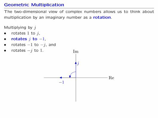
Geometric Multiplication
The two-dimensional view of complex numbers allows us to think about
multiplication by an imaginary number as a rotation.
Multiplying by j
• rotates 1 to j,
• rotates j to −1,
• rotates −1 to −j, and
• rotates −j to 1.
Re
Im
j
−1
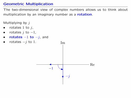
Geometric Multiplication
The two-dimensional view of complex numbers allows us to think about
multiplication by an imaginary number as a rotation.
Multiplying by j
• rotates 1 to j,
• rotates j to −1,
• rotates −1 to −j, and
• rotates −j to 1.
Re
Im
−1
−j

Geometric Multiplication
The two-dimensional view of complex numbers allows us to think about
multiplication by an imaginary number as a rotation.
Multiplying by j
• rotates 1 to j,
• rotates j to −1,
• rotates −1 to −j, and
• rotates −j to 1.
Re
Im
1
−j

Geometric Multiplication
The two-dimensional view of complex numbers allows us to think about
multiplication by an imaginary number as a rotation.
Multiplying by j
• rotates 1 to j,
• rotates j to −1,
• rotates −1 to −j, and
• rotates −j to 1.
Re
Im
1
j
−1
Multiplying by j rotates a vector by π/2.
Multiplying by j2 = −1 rotates a vector by π.

Geometric Multiplication
Multiplying by j rotates an arbitrary complex number by π/2.
c = a+ jb
jc = ja− b
Re
Im
jc
c
a−b
b
a
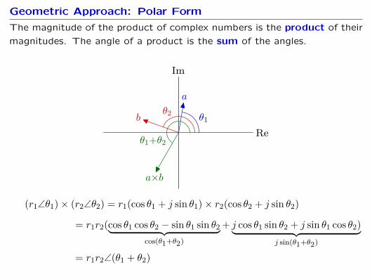
Geometric Approach: Polar Form
The magnitude of the product of complex numbers is the product of their
magnitudes. The angle of a product is the sum of the angles.
Re
Im
a
b
a×b
θ1θ2
θ1+θ2
(r1∠θ1)× (r2∠θ2) = r1(cos θ1 + j sin θ1)× r2(cos θ2 + j sin θ2)
= r1r2(cos θ1 cos θ2 − sin θ1 sin θ2︸ ︷︷ ︸cos(θ1+θ2)
+ j cos θ1 sin θ2 + j sin θ1 cos θ2)︸ ︷︷ ︸j sin(θ1+θ2)
= r1r2∠(θ1 + θ2)

Geometric Interpretation of Euler’s Formula
Euler’s formula equates polar and rectangular descriptions of a unit vector
at angle θ.
ejθ = cos θ + j sin θ
θRe
Im
cos θ
sinθ1
ejθ = cos θ + j sin θ
This interpretation came nearly 150 years after Euler’s formulation.
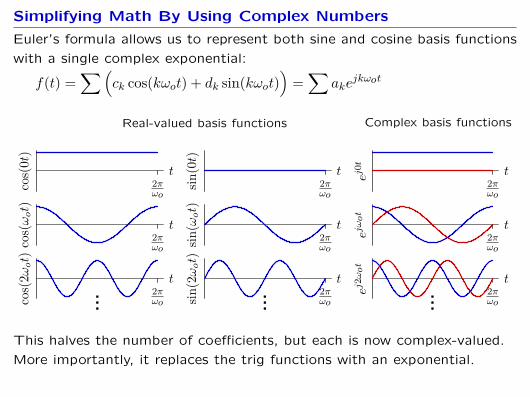
Simplifying Math By Using Complex Numbers
Euler’s formula allows us to represent both sine and cosine basis functions
with a single complex exponential:
f(t) =∑(
ck cos(kωot) + dk sin(kωot))
=∑
akejkωot
2πωo
t
cos(
0t)
2πωo
t
sin(0t)
2πωo
tej0t
2πωo
t
cos(ωot)
2πωo
t
sin(ω
ot)
2πωo
t
ejωot
2πωo
t
cos(
2ωot)
...2πωo
t
sin(2ωot)
...2πωo
t
ej2ωot
...
Real-valued basis functions Complex basis functions
This halves the number of coefficients, but each is now complex-valued.
More importantly, it replaces the trig functions with an exponential.

Converting From Trig Form To Complex Exponential Form
Assume that a function f(t) can be written as a Fourier series in trig form.
f(t) = f(t+ T ) = c0 +∞∑k=1
(ck cos(kωot) + dk sin(kωot)
)We can use Euler’s formula to convert sinusoids to complex exponentials.
ejkωot = cos(kωot) + j sin(kωot)cos(kωot) = Re{ejkωot} = (ejkωot + e−jkωot)/2sin(kωot) = Im{ejkωot} = −j(ejkωot − e−jkωot)/2
f(t) = c0+12
∞∑k=1
(cke
jkωot+cke−jkωot−jdkejkωot+jdke−jkωot)
= co+12
∞∑k=1
(ck−jdk)ejkωot+12
∞∑k=1
(ck+jdk)e−jkωot
= co+12
∞∑k=1
(ck−jdk)ejkωot+12
−∞∑k=−1
(c−k+jd−k)ejkωot =∞∑
k=−∞ake
jkωot
where ak ={ (ck − jdk)/2 if k > 0
c0 if k = 0(c−k + jd−k)/2 if k < 0

Negative Frequencies
The complex form of a Fourier series has both positive and negative k’s.
Only positive values of k are used in the trig form:
f(t) = c0 +∞∑k=1
ck cos(kωot) +∞∑k=1
dk sin(kωot)
but both positive and negative values of k are used in the exponential form:
f(t) =∞∑
k=−∞ake
jkωot
If we only included positive k in the previous sum, the result would always
have an imaginary component (unless ak = 0 for all k).
If f(t) is real-valued (as it must be for the trig form), then the complex
coefficients ak are conjugate symmetric:
a−k = a∗k
where the ∗ denotes the complex conjugate.
k : . . . −3 −2 −1 0 1 2 3 . . .
ak : . . .c3+jd3
2c2+jd2
2c1+jd1
2 c0c1−jd1
2c2−jd2
2c3−jd3
2 . . .

Fourier Series Directly From Complex Exponential Form
Assume that f(t) is periodic in T and is composed of a weighted sum of
harmonically related complex exponentials.
f(t) = f(t+ T ) =∞∑
k=−∞ake
jωokt
We can “sift” out the component at lωo by multiplying both sides by e−jlωot
and integrating over a period.
∫Tf(t)e−jωoltdt =
∫T
∞∑k=−∞
akejωokte−jωoltdt =
∞∑k=−∞
ak
∫Te jωo(k−l)tdt
={Tal if l = k
0 otherwise
Solving for al provides an explicit formula for the coefficients:
ak = 1T
∫Tf(t)e−jωoktdt ; where ωo = 2π
T.
This formulation works even if f(t) has complex values.

Orthogonality and Projection
Fourier components are separable because they are orthogonal.
Similar to separating a vector r into x and y components.
Since x and y are orthogonal, we can separate the x and y components of
r by projection:
a= r · xb= r · y
Then
r= ax+ by
x
y
a
rb

Orthogonal Decompositions
Vector representation: let r represent a vector with components a and b
in the x and y directions, respectively.
a = r · xb = r · y (“analysis” equations)
r = ax + by (“synthesis” equation)
ak=1T
∫Tf(t)e−j
2πTktdt (“analysis” equation)
f(t)= f(t+ T ) =∞∑
k=−∞ake
j 2πTkt (“synthesis” equation)

Orthogonal Decompositions
Vector representation: let r represent a vector with components a and b
in the x and y directions, respectively.
a = r · xb = r · y (“analysis” equations)
r = ax + by (“synthesis” equation)
Fourier series: let f(t) represent a signal with harmonic components
a0, a1, . . ., ak for harmonics e j0t, e j2πTt, . . ., e j
2πTkt respectively.
ak=1T
∫Tf(t)e−j
2πTktdt (“analysis” equation)
f(t)= f(t+ T ) =∞∑
k=−∞ake
j 2πTkt (“synthesis” equation)
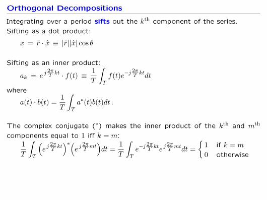
Orthogonal Decompositions
Integrating over a period sifts out the kth component of the series.
Sifting as a dot product:
x = r · x ≡ |r||x| cos θ
Sifting as an inner product:
ak = e j2πTkt · f(t) ≡ 1
T
∫Tf(t)e−j
2πTktdt
where
a(t) · b(t) = 1T
∫Ta∗(t)b(t)dt .
The complex conjugate (∗) makes the inner product of the kth and mth
components equal to 1 iff k = m:1T
∫T
(e j
2πTkt)∗(
e j2πTmt)dt = 1
T
∫Te−j
2πTkte j
2πTmtdt =
{1 if k = m
0 otherwise
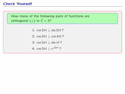
Check Yourself
How many of the following pairs of functions are
orthogonal (⊥) in T = 3?
1. cos 2πt ⊥ sin 2πt ?
2. cos 2πt ⊥ cos 4πt ?
3. cos 2πt ⊥ sin πt ?
4. cos 2πt ⊥ e j2πt ?
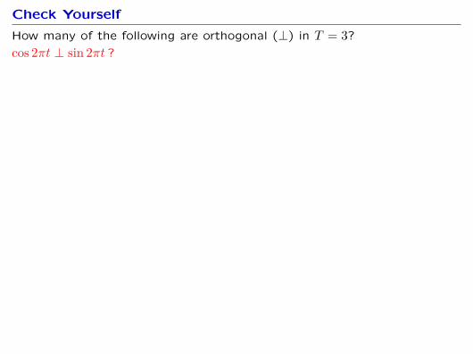
Check Yourself
How many of the following are orthogonal (⊥) in T = 3?
cos 2πt ⊥ sin 2πt ?

Check Yourself
How many of the following are orthogonal (⊥) in T = 3?
cos 2πt ⊥ sin 2πt ?
1 2 3t
cos 2πt
1 2 3t
sin 2πt
1 2 3t
cos 2πt sin 2πt = 12 sin 4πt
∫ 3
0dt = 0 therefore YES

Check Yourself
How many of the following are orthogonal (⊥) in T = 3?
cos 2πt ⊥ cos 4πt ?

Check Yourself
How many of the following are orthogonal (⊥) in T = 3?
cos 2πt ⊥ cos 4πt ?
1 2 3t
cos 2πt
1 2 3t
cos 4πt
1 2 3t
cos 2πt cos 4πt = 12 cos 6πt+ 1
2 cos 2πt
∫ 3
0dt = 0 therefore YES

Check Yourself
How many of the following are orthogonal (⊥) in T = 3?
cos 2πt ⊥ sin πt ?

Check Yourself
How many of the following are orthogonal (⊥) in T = 3?
cos 2πt ⊥ sin πt ?
1 2 3t
cos 2πt
1 2 3t
sin πt
1 2 3t
cos 2πt sin πt = 12 sin 3πt− 1
2 sin πt
∫ 3
0dt 6= 0 therefore NO

Check Yourself
How many of the following are orthogonal (⊥) in T = 3?
cos 2πt ⊥ ej2πt ?

Check Yourself
How many of the following are orthogonal (⊥) in T = 3?
cos 2πt ⊥ ej2πt ?
e2πt = cos 2πt+ j sin 2πt
cos 2πt ⊥ sin 2πt but not cos 2πtTherefore NO

Check Yourself
How many of the following pairs of functions
are orthogonal (⊥) in T = 3? 2
1. cos 2πt ⊥ sin 2πt ?√
2. cos 2πt ⊥ cos 4πt ?√
3. cos 2πt ⊥ sin πt ? X
4. cos 2πt ⊥ e j2πt ? X

Fourier Series
Comparison of trigonometric and complex exponential forms.
Complex Exponential Form
f(t) = f(t+ T ) =∞∑
k=−∞ake
jkωot
ak = 1T
∫Tf(t)e−jkωotdt
Trigonometric Form
f(t) = f(t+ T ) = co +∞∑k=1
ck cos(kωot) +∞∑k=1
dk sin(kωot)
c0 = 1T
∫Tf(t) dt
ck = 2T
∫T
cos(kωot) dt; k = 1, 2, 3, . . .
dk = 2T
∫T
sin(kωot) dt; k = 1, 2, 3, . . .

Comparison of Trigonometric and Complex Exponential Forms
It seems as though it takes more numbers to characterize the complex
exponential form:
• Each harmonic frequency in the complex exponential form depends on
two complex-valued numbers: ak and a−k.
• Each harmonic frequency in the trig form depends on two real-valued
numbers: ck and dk.
Q: What is going on?
A: The complex exponential form allows f(t) to have complex values.
The trigonometic form requires that f(t) be real-valued.
Q: Isn’t it twice the work to compute both ak and a−k?
A: Only if f(t) is complex-valued.
If f(t) is real-valued, then a−k is the complex conjugate of ak.

Is the Complex Exponential Form Actually Easier?
Last week, we determined the effect of a half-period shift on the Fourier
coefficients of the trig form. The result was a bit complicated.
Assume that f(t) is periodic in time with period T :
f(t) = f(t+ T ) .Let g(t) represent a version of f(t) shifted by half a period:
g(t) = f(t− T/2) .
How many of the following statements correctly describe the
effect of this shift on the Fourier series coefficients.
• cosine coefficients ck are negated X
• sine coefficients dk are negated X
• odd-numbered coefficients c1, d1, c3, d3, . . . are negated√
• sine and cosine coefficients are swapped: ck → dk and dk → ck X

Half-Period Shift
Shifting f(t) shifts the underlying basis functions of it Fourier expansion.
f(t− T/2) =∞∑k=0
ck cos (kωo(t− T/2)) +∞∑k=1
dk sin (kωo(t− T/2))
2πωo
t
cos(
0t)
cosine basis functions
2πωo
t
delayed half a period
2πωo
t
cos(ωot)
2πωo
t
2πωo
t
cos(
2ωot)
2πωo
t
2πωo2πωo
tt
cos(
3ωot)
...2πωo...
Half-period shift inverts ck terms if k is odd. It has no effect if k is even.

Half-Period Shift
Shifting f(t) shifts the underlying basis functions of it Fourier expansion.
f(t− T/2) =∞∑k=0
ck cos (kωo(t− T/2)) +∞∑k=1
dk sin (kωo(t− T/2))
2πωo
t
sin(0t)
sine basis functions
2πωo
t
delayed half a period
2πωo
t
sin(ω
ot)
2πωo
t
2πωo
t
sin(2ωot)
2πωo
t
2πωo2πωo
tt
sin(3ωot)
...2πωo...
Half-period shift inverts dk terms if and only if k is odd.

Quarter-Period Shift
Shifting by T/4 is even more complicated.
f(t− T/4) =∞∑k=0
ck cos (kωo(t− T/4)) +∞∑k=1
dk sin (kωo(t− T/4))
2πωo
t
cos(
0t)
cosine basis functions
2πωo
t
delayed one fourth period
2πωo
t
cos(ωot)
2πωo
t
2πωo
t
cos(
2ωot)
2πωo
t
2πωo2πωo
tt
cos(
3ωot)
...2πωo...
cos(ωot)→ sin(ωot); cos(2ωot)→ − cos(2ωot); cos(3ωot)→ − sin(3ωot)

Check Yourself: Alternative (more intuitive) Approach
Shifting f(t) shifts the underlying basis functions of it Fourier expansion.
f(t− T/4) =∞∑k=0
ck cos (kωo(t− T/4)) +∞∑k=1
dk sin (kωo(t− T/4))
2πωo
t
sin(0t)
sine basis functions
2πωo
t
delayed 1/4 period
2πωo
t
sin(ω
ot)
2πωo
t
2πωo
t
sin(2ωot)
2πωo
t
2πωo2πωo
tt
sin(3ωot)
...2πωo...
sin(ωot)→ − cos(ωot); sin(2ωot)→ − sin(2ωot); sin(3ωot)→ cos(3ωot)

Summary of Shift Results
Let ck and dk represent the Fourier series coefficients for f(t)
f(t) = f(t+ T ) = c0 +∞∑k=1
ck cos(kωot) +∞∑k=1
dk sin(kωot)
and c′k and d′k represent those for a half-period delay.
g(t) = f(t− T/2) = c0 +∞∑k=1
c′k cos(kωot) +∞∑k=1
d′k sin(kωot)
Then c′k = (−1)kck and d′k = (−1)kdk.
Let c′′k and d′′k represent those for a quarter-period delay.
g(t) = f(t− T/2) = c0 +∞∑k=1
c′k cos(kωot) +∞∑k=1
d′k sin(kωot)
Then
c′′k =
ck if k = 0, 4, 8, 12, . . .dk if k = 1, 5, 9, 13, . . .−ck if k = 2, 6, 10, 14, . . .−dk if k = 3, 7, 11, 15, . . .
d′′k =
dk if k = 0, 4, 8, 12, . . .−ck if k = 1, 5, 9, 13, . . .−dk if k = 2, 6, 10, 14, . . .ck if k = 3, 7, 11, 15, . . .

Other Shifts Yield Even More Complicated Results
Let ck and dk represent the Fourier series coefficients for f(t)
f(t) = f(t+ T ) = c0 +∞∑k=1
ck cos(kωot) +∞∑k=1
dk sin(kωot)
and c′′′k and d′′′k represent those for n eighth-period delay.
g(t) = f(t− T/8) = c0 +∞∑k=1
c′k cos(kωot) +∞∑k=1
d′k sin(kωot)
c′′′k =
ck if k = 0, 8, 16, 24, . . .√
22 (ck + dk) if k = 1, 9, 17, 25, . . .
dk if k = 2, 10, 18, 26, . . .√
22 (−ck + dk) if k = 3, 11, 19, 27, . . .
−ck if k = 4, 12, 20, 28, . . .√
22 (−ck − dk) if k = 5, 13, 21, 29, . . .
−dk if k = 6, 14, 22, 30, . . .√
22 (ck − dk) if k = 7, 15, 23, 31, . . .
d′′′k = . . .

Effects of Time Shifts on Complex Exponential Series
Delaying time by τ multiplies the complex exponential coefficients of a
Fourier series by a constant e−jkωoτ .
Let ak represent the complex exponential series coefficients of f(t) and a′krepresent the complex exponential series coefficents of g(t) = f(t− τ).
a′k = 1T
∫Tg(t)e−jkωotdt
= 1T
∫Tf(t− τ)e−jkωotdt
= 1T
∫Tf(s)e−jkωo(s+τ)ds
= e−jωoτ1T
∫Tf(s)e−jkωosds
= e−jkωoτak
Each coefficient a′k in the series for g(t) is a constant e−jkωot times the
corresponding coefficient ak in the series for f(t).

Summary
We introduced the complex exponential form of Fourier series.
• complex numbers, complex exponentials, and their relation to sinusoids
• analysis and synthesis with complex exponentials
• delay property: much simpler with complex exponentials
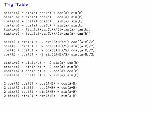
Trig Table
sin(a+b) = sin(a) cos(b) + cos(a) sin(b)sin(a-b) = sin(a) cos(b) - cos(a) sin(b)cos(a+b) = cos(a) cos(b) - sin(a) sin(b)cos(a-b) = cos(a) cos(b) + sin(a) sin(b)tan(a+b) = (tan(a)+tan(b))/(1-tan(a) tan(b))tan(a-b) = (tan(a)-tan(b))/(1+tan(a) tan(b))
sin(A) + sin(B) = 2 sin((A+B)/2) cos((A-B)/2)sin(A) - sin(B) = 2 cos((A+B)/2) sin((A-B)/2)cos(A) + cos(B) = 2 cos((A+B)/2) cos((A-B)/2)cos(A) - cos(B) = -2 sin((A+B)/2) sin((A-B)/2)
sin(a+b) + sin(a-b) = 2 sin(a) cos(b)sin(a+b) - sin(a-b) = 2 cos(a) sin(b)cos(a+b) + cos(a-b) = 2 cos(a) cos(b)cos(a+b) - cos(a-b) = -2 sin(a) sin(b)
2 cos(A) cos(B) = cos(A-B) + cos(A+B)2 sin(A) sin(B) = cos(A-B) - cos(A+B)2 sin(A) cos(B) = sin(A+B) + sin(A-B)2 cos(A) sin(B) = sin(A+B) - sin(A-B)