fourier analysis made easy - complex to real · fourier analysis made easy jean baptiste joseph,...
TRANSCRIPT

1Charan Langton, www.complextoreal.com
Fourier Analysis Made Easy
Jean Baptiste Joseph, Baron de Fourier, 1768 - 1830
While studying heat conduction in materials, Baron Fourier (a title given to him by Napoleon) developed his now famous Fourier series approximately 120 years after Newton published the first book on Calculus. It took him another twenty years to develop the Fourier transform which made the theory applicable to a variety of disciplines such as signal processing where Fourier analysis is now an essential tool. It seems that Fourier did little to develop the concept further and most of this work was done by Euler, LaGrange, Laplace and others. Fourier analysis is now also used heavily in communication, thermal analysis, image and signal processing, quantum mechanics and physics.
Fourier noticed that you can create some really interesting looking waves by just summing up simple sine and cosine waves. For example the wave in Figure 1, is a sum of the three sine waves shown in Figure 2 of various frequencies and amplitudes. From just this observation, Fourier correctly surmised that all kinds of interesting and useful waves could probably be created just by combining sines and cosines.
Figure 1 - An interesting looking wave
Figure 2 - Sine wave 1, Sine wave 2, Sine wave 3
So although we know that the wave of Figure 1 is created from the sum or superposition of the three regular looking waves shown in Figure 2, we can represent this knowledge in a more interesting way. Let’s look at the composite wave in three dimensions. When we look at the signal with time progressing to the right and the amplitude going up and down erratically, we are looking at the signal in what is called, the Time Domain. This is the summed signal. When we look at the same signal from the “side”, along the

2Charan Langton, www.complextoreal.com
frequency axis, now what we see are the constituent frequencies along the frequency axis. We also see the peak amplitudes of these discrete frequencies. This view of the signal is called the Frequency Domain. Another name for this view is the Signal Spectrum.
Figure 3 - Looking at signals from two different points of view
The concept of spectrum comes about from the realization that any arbitrary wave contains within it many different frequencies. A real signal of any type is an assemblage of all kinds of frequencies. Examples of such a signals is voice, which varies in frequency from 30 Hz to 10000 Hz. Although the range of frequencies is the same for most humans, the distribution of powers is different and results in a unique and recognizable sound. The spectrum is a way to quantify the power within each of the component frequencies.
The spectrum of the composite wave of Figure 1 is composed of just three frequencies and can be visualized in Frequency domain as in Figure 4. This view is called a one-sided spectrum. One-sided not because any thing has been left out of it, but that only positive frequencies are represented. (So what is a negative frequency? Is there such a thing? We will discuss this in more detail in chapter 2.)
Figure 4 - The Frequency Domain spectrum of wave in Figure 1
The x-axis in this spectrum represents the frequencies and y-axis is the amplitude or power in those frequencies. Typically a spectrum represents power, so the y-axis value is the peak amplitude squared, hence it is always a positive quantity. But often it is called amplitude, although technically this is not correct. The width of the spectrum is called the bandwidth of the signal and the resolution of the
3Charan Langton, www.complextoreal.com
frequencies ( )1n nf f+ − is called the bin size. The bin size of a spectrum is constant and is an important parameter in how well the signal has been represented.
The smallest frequency (which has the largest amplitude in Figure 4) is called the Fundamental Frequency. All other frequencies are integer multiples of this fundamental frequency in the analysis we are about to undertake. So if the smallest frequency in a spectrum is 21.3 Hz, then the next harmonic would be 2 times that. The bin size in this case would be 21.3 Hz as well.
A spectrum is a graphical representation of the power content of the fundamental frequency and all its harmonic or integer multiples. This graphical representation is a unique signature of the signal at a particular time. A spectrum hence is not a static thing and changes as the signal changes.
The process of breaking down any arbitrary wave into its harmonic components and identifying their contents, that is their amplitudes, is called Fourier Analysis.
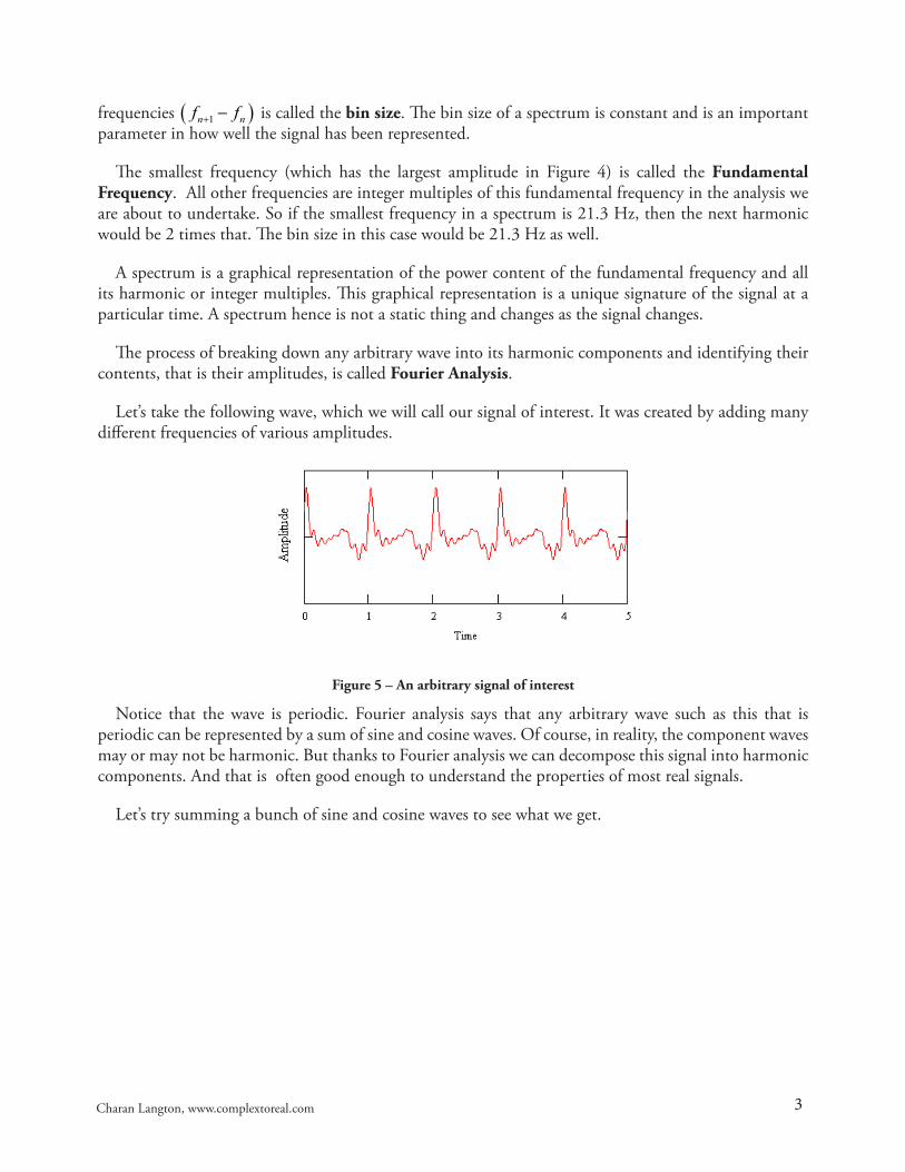
Let’s take the following wave, which we will call our signal of interest. It was created by adding many different frequencies of various amplitudes.
Figure 5 – An arbitrary signal of interest
Notice that the wave is periodic. Fourier analysis says that any arbitrary wave such as this that is periodic can be represented by a sum of sine and cosine waves. Of course, in reality, the component waves may or may not be harmonic. But thanks to Fourier analysis we can decompose this signal into harmonic components. And that is often good enough to understand the properties of most real signals.
Let’s try summing a bunch of sine and cosine waves to see what we get.
4Charan Langton, www.complextoreal.com
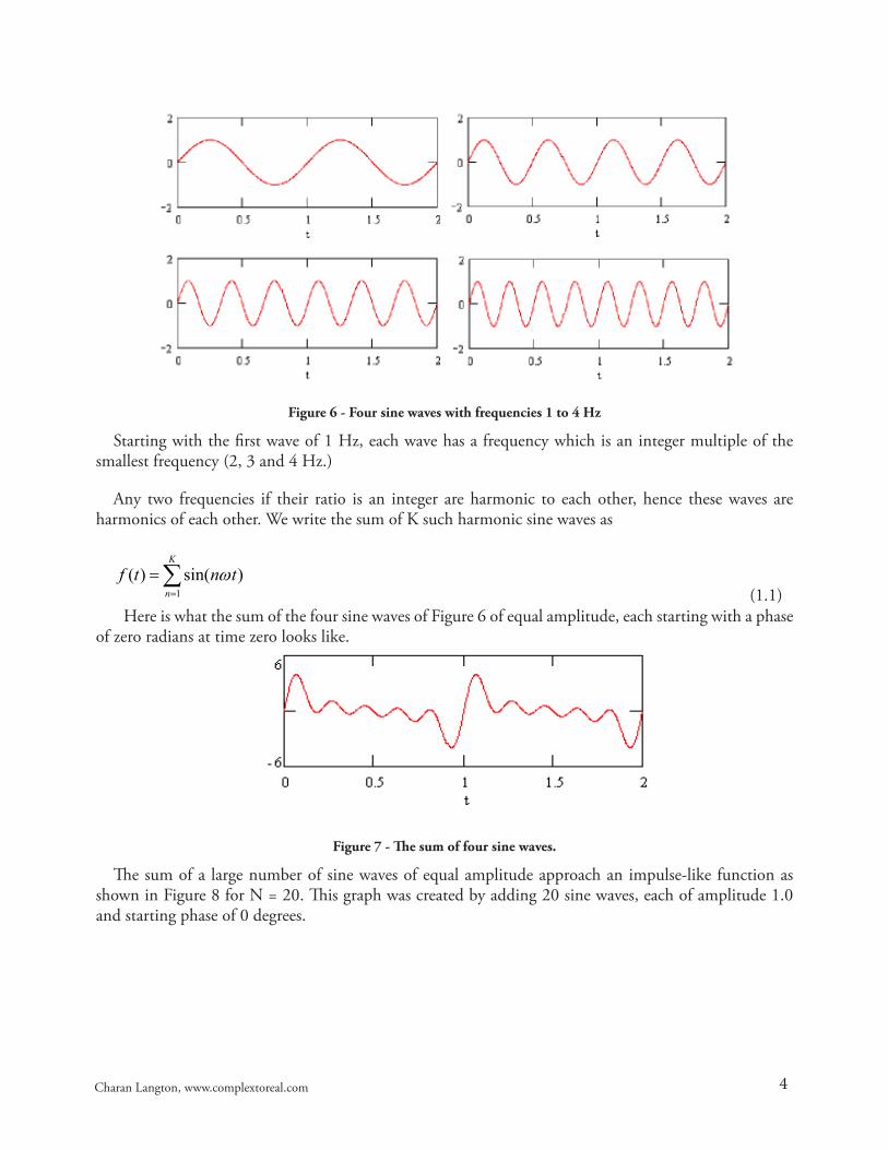
Figure 6 - Four sine waves with frequencies 1 to 4 Hz
Starting with the first wave of 1 Hz, each wave has a frequency which is an integer multiple of the smallest frequency (2, 3 and 4 Hz.)
Any two frequencies if their ratio is an integer are harmonic to each other, hence these waves are harmonics of each other. We write the sum of K such harmonic sine waves as
1( ) sin( )
K
nf t n tω
=
=∑ (1.1)
Here is what the sum of the four sine waves of Figure 6 of equal amplitude, each starting with a phase of zero radians at time zero looks like.
Figure 7 - The sum of four sine waves.
The sum of a large number of sine waves of equal amplitude approach an impulse-like function as shown in Figure 8 for N = 20. This graph was created by adding 20 sine waves, each of amplitude 1.0 and starting phase of 0 degrees.

5Charan Langton, www.complextoreal.com
Figure 8 - The sum of 20 harmonic sine waves.
We see two interesting things, one that the peak value is not the sum of the number of harmonics. The maximum amplitude is not equal to 20. Sine waves of harmonic frequencies do not have synchronous peaks. So the peak never adds to a linear sum of the amplitudes. This because all harmonic sine waves cross the x-axis at the same time but never peak at the same time, as opposed to cosine waves which peak at the same time but never cross the x-axis at the same time as we can see in Figures 9 and 10 .
The closed form solution of this summation is given by the following equation.
( )
0
1 1sin sin 12 2sin( )
1sin2
N
n
N Nn
N
ω ωω
ω=
+ =
∑ (1.2)
Figure 9 – These three harmonic sine waves all start at 0, and cross the x-axis at the same time. Note they all start at zero.
Figure 10 – Harmonic cosine waves peak synchronously. Note they all start at 1.0
Sine waves are considered odd functions from the following definition.
( ) ( )f x f x= − − (1.3)
6Charan Langton, www.complextoreal.com
Cosine waves are called even functions by a similar definition.
( ) ( )f x f x= − (1.4)
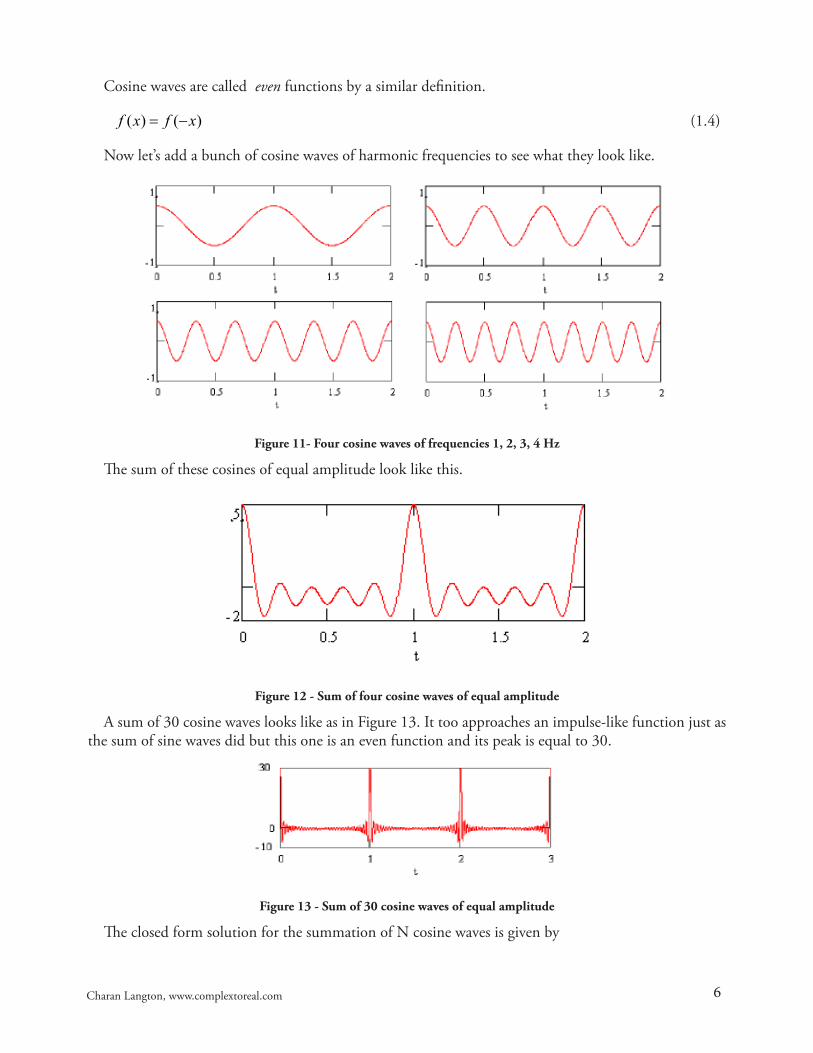
Now let’s add a bunch of cosine waves of harmonic frequencies to see what they look like.
Figure 11- Four cosine waves of frequencies 1, 2, 3, 4 Hz
The sum of these cosines of equal amplitude look like this.
Figure 12 - Sum of four cosine waves of equal amplitude
A sum of 30 cosine waves looks like as in Figure 13. It too approaches an impulse-like function just as the sum of sine waves did but this one is an even function and its peak is equal to 30.
Figure 13 - Sum of 30 cosine waves of equal amplitude
The closed form solution for the summation of N cosine waves is given by
7Charan Langton, www.complextoreal.com
( )
0
1 1cos sin 12 2cos( )
1sin2
N
n
N Nn
N
ω ωω
ω=
+ =
∑ (1.5)
Now let’s allow the amplitude of the cosine and sine waves to vary. Here is what one particular sum of four cosines and sines of unequal amplitude looks like.
Figure 14 - Sum of four cosine waves and sine waves of unequal amplitude.
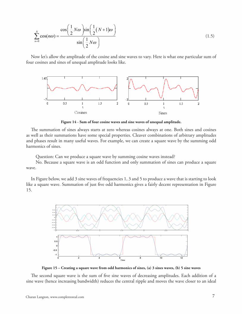
The summation of sines always starts at zero whereas cosines always at one. Both sines and cosines as well as their summations have some special properties. Cleaver combinations of arbitrary amplitudes and phases result in many useful waves. For example, we can create a square wave by the summing odd harmonics of sines.
Question: Can we produce a square wave by summing cosine waves instead?No. Because a square wave is an odd function and only summation of sines can produce a square
wave.
In Figure below, we add 3 sine waves of frequencies 1, 3 and 5 to produce a wave that is starting to look like a square wave. Summation of just five odd harmonics gives a fairly decent representation in Figure 15.
0 0.5 1 1.5 2 2.5 3-1
-0.8
-0.6
-0.4
-0.2
0
0.2
0.4
0.6
Figure 15 – Creating a square wave from odd harmonics of sines, (a) 3 sines waves, (b) 5 sine waves
The second square wave is the sum of five sine waves of decreasing amplitudes. Each addition of a sine wave (hence increasing bandwidth) reduces the central ripple and moves the wave closer to an ideal

8Charan Langton, www.complextoreal.com
square wave. The equation below gives the recipe of how this wave was created. The square wave is an odd function, so it can only be created from sine waves which have the necessary property of oddness. The even functions on the other hand can only be created using cosine waves. Non-symmetric signal representation would require both sines and cosines, such as for the signal in Figure 5.
Here is the expression for creating a square pulse from the summation of sine waves.
( )( )
( )1
sin 2 2 14( )2 1
4 1 1sin(2 ) sin(6 ) sin(10 )3 5
k
k ftsquare t
k
f t f t f t
ππ
π π ππ
∞
=
−=
−
= + + +
∑
(1.6)
Let’s look at two more special signals, triangular wave and sawtooth wave.
( ) ( )( )( )22
0
2
sin 2 2 18( ) 12 1
8 1 1sin(2 ) sin(6 ) sin(10 )9 25
k
k
k fttraingle t
k
f t f t f t
ππ
π π ππ
∞
=
+= −
+
= − + +
∑
(1.7)
Just looking at this equation, without knowing what it looks like, we know that since only sines are involved, this must be a odd function. The number of harmonics used to create the signal also tells us something of its bandwidth. A perfect reconstruction requires infinite number of harmonics which means infinite bandwidth.
Figure 16 – Triangular wave represented by sines
A triangular wave is also an odd function, which means it is constituted only of sine waves.
( ) 1
1
2 sin(2 )( ) 1 k
k
kftsawtooth tkπ
π
∞+
=
= −∑ (1.8)
Rectified wave – This is an even function, so we have only the cosines in the equation
( )
( )0
21
cos 22 4( )4 1n
f tA Af tnπ
π π
∞
=
= −−
∑ (1.9)

9Charan Langton, www.complextoreal.com
Figure 17 – Rectified wave represented by cosines
Fourier Series
Now we will put together what we have learned about harmonics for the creation of a general equation which can be used to represent any arbitrary periodic wave.
Let’s start with the two basic equations that sum harmonic frequencies of sines and cosines of equal amplitudes.
( )11
( ) sin 2n
f t n f tπ∞
=
=∑ (1.10)
( )21
( ) cos 2n
f t n f tπ∞
=
=∑ (1.11)
Here f is the fundamental frequency. We can also write these equations instead as
( )11
( ) sin 2 nn
f t f tπ∞
=
=∑ (1.12)
( )21
( ) cos 2 nn
f t f tπ∞
=
=∑ (1.13)
Where nf is the nth harmonic of the fundamental. Both of these equations can create a certain class of signals, such as odd or even. We already know what these summations look like. No matter how many sine waves we add, the starting point will always be zero. So if we want to create a wave that does not start at zero like the one in Figure 5, then we must include cosine waves in the formulation. We also understand that we need to allow the amplitudes to vary if we are to create anything interesting. Summation of equal amplitude sines and cosines are not interesting. By allowing the amplitude to vary, we can create a huge variety of waves, both odd, even and those with no symmetry.
Now let’s include both sines and cosines in one equation, allowing their amplitudes to vary by adding a different coefficient for each.

10Charan Langton, www.complextoreal.com
1 1
( ) sin(2 ) cos(2 )N N
n n n nn n
f t a f t b f tπ π= =
= +∑ ∑ (1.14)
The coefficients an represent the coefficient of the nth sine wave and bn of the nth cosine wave.
There is one other issue to tackle if we are to make this formula truly general, capable of representing all kinds of waves. The sum of sine and cosines is always symmetrical about the x-axis so there is no possibility of representing a wave with a dc offset. To do that we must add a bias to Equation (1.14). The constant, 0a we add to Equation (1.14) moves the whole wave up (or down) from the x-axis.
01 1
( ) sin(2 ) cos(2 )N N
n n n nn n
f t a f b f ta π π= =
= + +∑ ∑ (1.15)
The coefficient a0 provides us with the needed dc offset. Now with this equation we can describe any periodic wave, no matter how complicated looking it is. We know that ultimately we can represent it with just ordinary sines and cosines.
Question: Can we create an exponential and other non-periodic functions with this formulation?No. In fact hidden in this formula are exponentials. We can use exponentials to create periodic
waves but not the other way around.
Equation (1.15) is called the Fourier series equation. The coefficients a0, an, bn are called the Fourier Series Coefficients.
An equation with many faces
There are several different ways to write the Fourier series equation. One common representation is by radial frequency. We can replace frequency by ω and then write the equation as
01 1
( ) sin( ) cos( )N N
n n n nn n
f t a a t b tω ω= =
= + +∑ ∑ (1.16)
For discrete representation, we define T as the period of the fundamental frequency (the lowest frequency in the set). Then the period of the nth harmonic is T/n and /nf n T= . We now write the Fourier equation as follows
01
( ) sin 2 cos 2n nn
n nf t a a t b tT T
π π∞
=
= + +∑ (1.17)
The cosine representation, used often in signal processing is written by incorporating a variable for the phase. Now sine wave is not necessary because by changing the phase we can create any wave.
01
( ) cos( )n n nn
f t C C w t φ∞
=
= + +∑ (1.18)
Here is one more way to write the same equation by pulling out the constant amplitude term to the front.

11Charan Langton, www.complextoreal.com
01
1( ) ( sin cos )2 n n n n
nf t a a f t b f t
π
∞
=
= + +∑ (1.19)
We can also write the equation starting at zero frequency. Now the bias term is included with the zero frequency.
0
1( ) ( sin cos )2 n n n n
nf t a f t b f t
π
∞
=
= +∑ (1.20)
Additionally in its most important representation, the complex representation, the Fourier Equation is written as
/( ) jn t Tn
nf t C e π
∞
=−∞
= ∑ (1.21)
This says that we can create a periodic function by the summations of exponentials. Complex notation is a most useful albeit a scary looking form. In next part, we will look at how it is derived and used for signal processing.
A beautiful example showing how a sine wave is actually the sum of very many exponentials is given by Kalid Azad at http://betterexplained.com/articles/intuitive-understanding-of-sine-waves.
Figure 18 - A sine wave as a summation of exponentials
We see that a sine wave is the sum of a linear function and then addition and subtractions of restoring forces in the opposite directions. Mathematically we see this in the following power series equation of a sine wave.
3 5 7
sin( )3! 5! 7!x x xx x= − + − + (1.22)
All these different representations of the Fourier Series are identical and mean exactly the same thing.
12Charan Langton, www.complextoreal.com
How to compute the Fourier Coefficients of a wave
In signal processing we are interested in spectral components of a signal. We want to know what the bandwidth is, and how the power is distributed over that bandwidth. When looking at a signal, we have no idea what its components are. So ho can we go about assessing the signal? Fourier analysis gives us a tool to do this. But Fourier analysis means breaking a signal down in harmonics. Real life is not made up of neat harmonics. So when we use Fourier analysis, we are deconstructing a signal into harmonic components which is a sort of an approximation of reality and not its true representation.
We are interested in knowing how many of the sines and cosines the target signal (Figure 5) can be represented by and what their amplitudes are. Alternatively, what we really want are the Fourier coefficients of the signal. Once we know the Fourier coefficients, we can draw the spectrum.
Question: What is the relationship of Fourier coefficients to the spectrum?The coefficients of the sine wave and the coefficients of the cosines, both represent the amplitudes
and hence power of a particular harmonic.
How do we compute the Fourier Coefficients? We will look at each of the three types of coefficients separately and see how they can be computed.
Computing a0 the dc coefficient
01
1( ) ( sin cos )2 n n n n
nf t a f ta t b f
π
∞
=
= + +∑ (1.23)
The constant a0 in the Fourier Equation represents the dc offset. It can also be called the bias. But before we compute it, let’s take a look at a useful property of the sine and cosine waves.
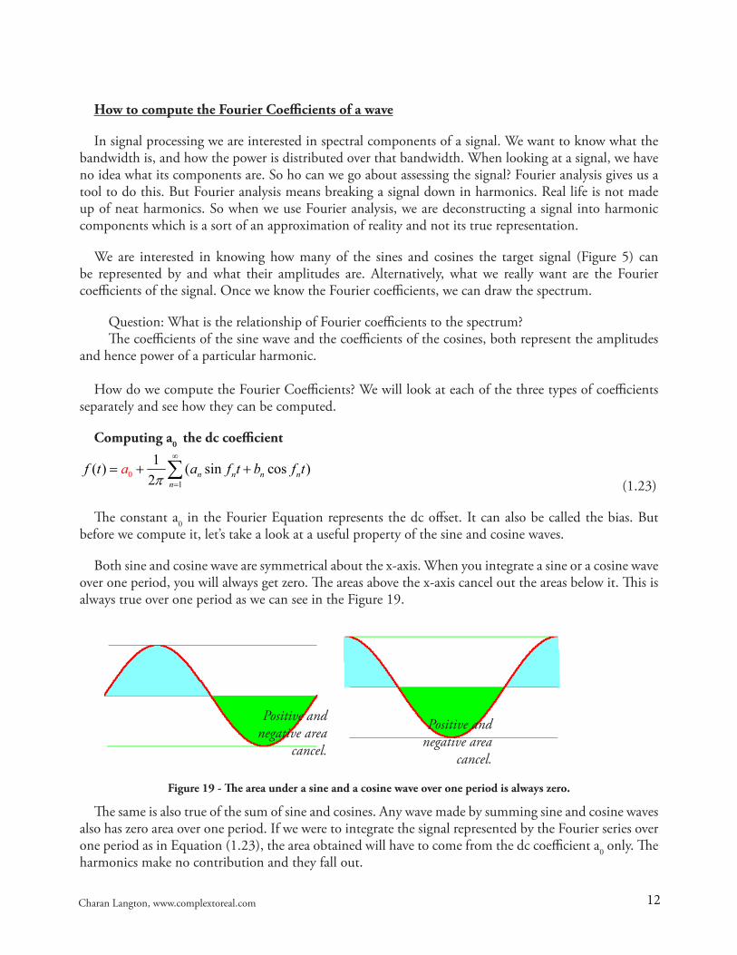
Both sine and cosine wave are symmetrical about the x-axis. When you integrate a sine or a cosine wave over one period, you will always get zero. The areas above the x-axis cancel out the areas below it. This is always true over one period as we can see in the Figure 19.
Figure 19 - The area under a sine and a cosine wave over one period is always zero.
The same is also true of the sum of sine and cosines. Any wave made by summing sine and cosine waves also has zero area over one period. If we were to integrate the signal represented by the Fourier series over one period as in Equation (1.23), the area obtained will have to come from the dc coefficient a0 only. The harmonics make no contribution and they fall out.
Positive and negative area
cancel.
Positive and negative area
cancel.
13Charan Langton, www.complextoreal.com
00 1
( s) in cosT
T
o
T
n non
a nwtf t dt b nwt ta dt d∞
=
= +
+ ∑∫ ∫ ∫
(1.24)
The second term is zero in Equation (1.24), since it is just the integral of a wave made up of sine and cosines.
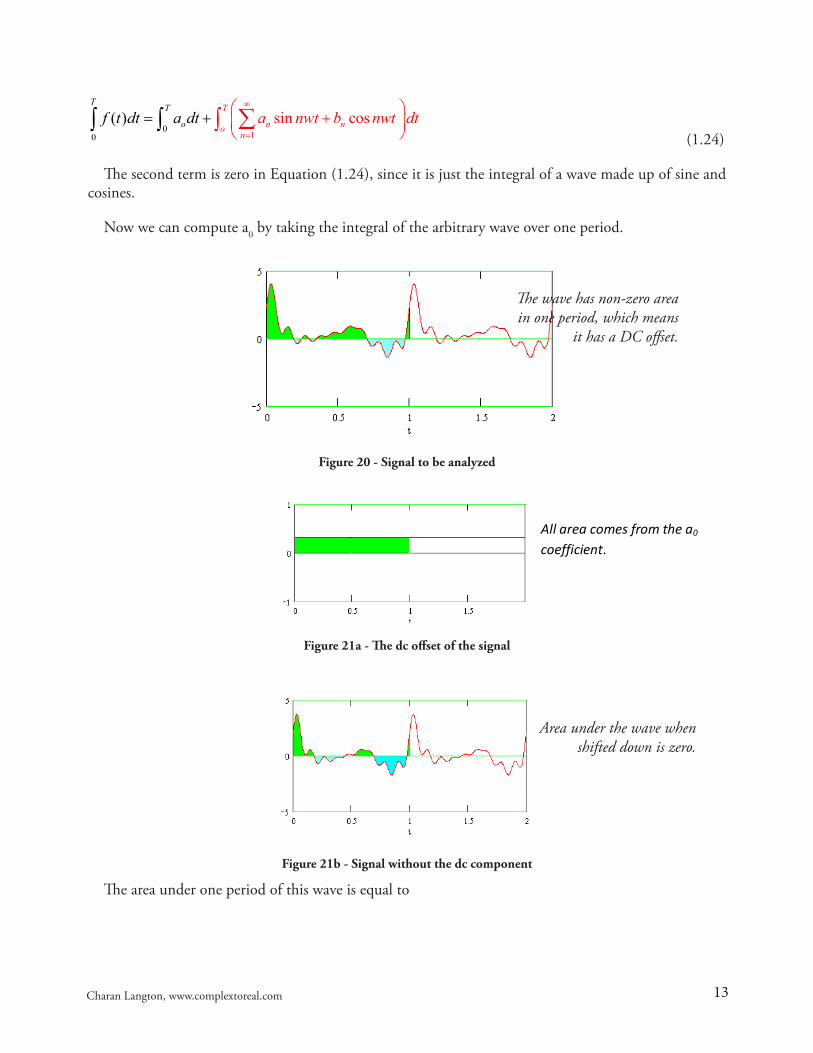
Now we can compute a0 by taking the integral of the arbitrary wave over one period.
Figure 20 - Signal to be analyzed
Figure 21a - The dc offset of the signal
Figure 21b - Signal without the dc component
The area under one period of this wave is equal to
The wave has non-zero area in one period, which means
it has a DC offset.
Area under the wave when shifted down is zero.
All area comes from the a0 coefficient.

14Charan Langton, www.complextoreal.com
00
( )T
T
of t dt a dt=∫ ∫ (1.25)
Integrating this very simple equation we get,
00
( )T
f t dt a T=∫ (1.26)
We can now write a very easy equation for computing
00
1 ( )T
a f t dtT
= ∫ (1.27)
Since no harmonics contribute to the area, we see that a0 is equal to simply the area under the wave for one period. We can compute this area in software and if it comes out zero, then there is no dc offset.
Computing na - the coefficients of sine waves
Now we employ a slightly different trick from basic trigonometry to compute the coefficients of the various sine waves. Below we show a sine wave that has been multiplied by itself.
Figure 22 - The area under a sine wave multiplied by itself is always non-zero.
We notice that the wave now lies entirely above the x-axis and has net positive area. From integral tables we can compute this area as equal to
0
sin sin / 2T
n na nwt nwt dt a T for n m= =∫ (1.28)
Now multiply the sine wave by an arbitrary harmonic of itself to see what happens to the area.
( ) sin sinf t n t n tω ω= ×
Multiplying one sine wave by any other causes the area
under the new wave to become zero.
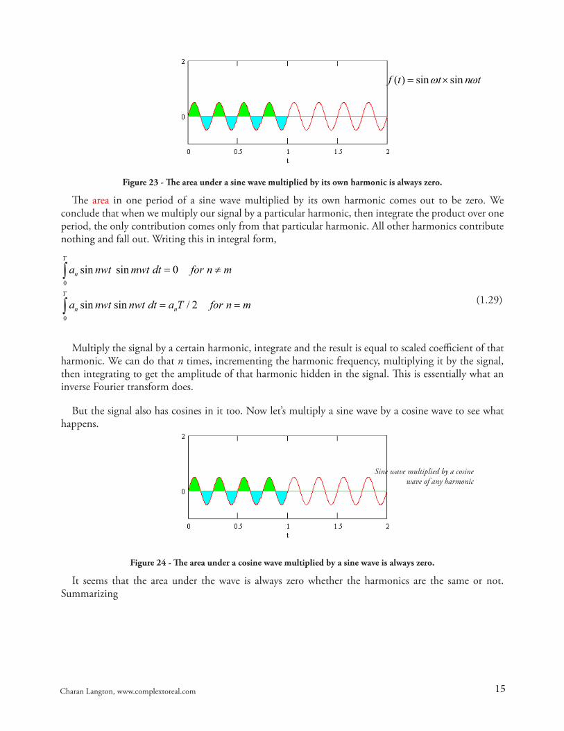
15Charan Langton, www.complextoreal.com
Figure 23 - The area under a sine wave multiplied by its own harmonic is always zero.
The area in one period of a sine wave multiplied by its own harmonic comes out to be zero. We conclude that when we multiply our signal by a particular harmonic, then integrate the product over one period, the only contribution comes only from that particular harmonic. All other harmonics contribute nothing and fall out. Writing this in integral form,
0
0
sin sin 0
sin sin / 2
T
n
T
n n
a nwt mwt dt for n m
a nwt nwt dt a T for n m
= ≠
= =
∫
∫ (1.29)
Multiply the signal by a certain harmonic, integrate and the result is equal to scaled coefficient of that harmonic. We can do that n times, incrementing the harmonic frequency, multiplying it by the signal, then integrating to get the amplitude of that harmonic hidden in the signal. This is essentially what an inverse Fourier transform does.
But the signal also has cosines in it too. Now let’s multiply a sine wave by a cosine wave to see what happens.
Figure 24 - The area under a cosine wave multiplied by a sine wave is always zero.
It seems that the area under the wave is always zero whether the harmonics are the same or not. Summarizing
Sine wave multiplied by a cosine wave of any harmonic
( ) sin sinf t t n tω ω= ×
16Charan Langton, www.complextoreal.com
0
0
0
sin sin 0
sin sin / 2
cos sin 0
T
n
T
n n
T
n
a nwt mwt dt for n m
a nwt nwt dt a T for n m
a nwt mwt dt
= ≠
= =
=
∫
∫
∫ (1.30)
Remember in vector representation sine and cosines are orthogonal to each other. This result tells us something about the orthogonality of sines and cosines. We are basically taking a dot product here. The dot product of a sine and cosine results in no area, hence the two signals are orthogonal. In fact all harmonics are orthogonal to each other. The dot product of two orthogonal waves is always zero which corroborates the above results. Another very satisfying interpretation is that sine wave and cosine waves act as filtering signals. In essence they act as a narrow-band filter and ignore all frequencies except the one of interest. This is the fundamental concept of a filter.
Now let’s use this information. Successively multiply the Fourier equation by a sine wave of a particular harmonic and integrate over one period as in equation below
00
0 sin cos si( )sin sin s0
in nT TT T
nno
f t nwt dt a na wt dt b nwt nwt d wt nwt dtt= + +∫∫∫ ∫ (1.31)
We know that the integral of the first and the third term is zero since the first term is just the integral of a sine wave multiplied by a constant and the third is of a sine wave multiplied by a cosine wave. This simplifies our equation considerably. We know that integral of the second term is
0
sin sin2
Tn
na Ta nwt nwt dt× =∫
(1.32)
From this we write the equation to obtain na as follows
0
2 ( ) sinT
na f t nwt dtT
= ∫ (1.33)
The coefficient na is hence computed by taking the target signal over one period, successively multiplying it with a sine wave of nth harmonic frequency and then integrating. This gives the coefficient for that particular harmonic. If we do this n times, we will get n coefficients.
Computing coefficient of cosines, bn
Now instead of multiplying by a sine wave we multiply by a cosine wave. The process is exactly the same as above.

17Charan Langton, www.complextoreal.com
0
00
co( )cos cs sin c os c s0
oosT TT
n
T
ona wt dt a nwf t nwt dt b nwt nwt dt nw t tt d= + ×× +∫ ∫ ∫ ∫
(1.34)
Now terms 1 and 2 become zero. The third terms as above is equal to
0
cos cos2
Tn
nb Tb nwt nwt dt× =∫
(1.35)
and the equation can be written as
0
2 ( ) cosT
nb f t nwt dtT
= ∫ (1.36)
So the process of finding the coefficients is multiplying the target signal with successively larger harmonic frequencies of a sine wave and integrating the results. This is easy to do in software. The result obtained is the coefficient for that particular frequency of sine wave. We do the same thing for cosine coefficients.
Let’s look at the signal from Figure 5. Here are the coefficients we used to create this signal.
na = [.4 .3 .7 .3 .3 .3 .2 .3 .4]
nb = [.05 .2 .7 .5 .2 .2 .1 .05 .02]
0a = .32
From this we can write the equation of the above wave as
. 4sin .3sin 2 .7sin 3 .3sin 4 .3sin 5 .3sin 6 .2sin 7 .3sin8 .4sin 9
.05cos .2cos 2 .7cos3 .5cos 4 .2cos5 .2cos 6 .1cos 7 .05cos8 .
(
01cos )
32) ..(
9t t t t tt t
f
t t tt t t t t
t
tt t
t+
+ + + + + + + + ++ + + +
=+ ++ + +
(1.37)
Conceptually the process of computing the coefficients consists of filtering the target signal one frequency at a time. In software when we compute the spectrum, this is exactly what we are doing. So the spectrum bins can be seen as tiny little filters.
Summary
The Fourier series is given by
01 1
( ) sin(2 ) cos(2 )N N
n n n nn n
f t a a f t b f tπ π= =
= + +∑ ∑ (1.38)
The coefficients in the Fourier series are given by
00
18Charan Langton, www.complextoreal.com
00
1 ( )T
a f t dtT
= ∫ (1.39)
0
2 ( ) sinT
na f t nwt dtT
= ∫ (1.40)
0
2 ( ) cosT
nb f t nwt dtT
= ∫ (1.41)
Coefficients become the spectrum
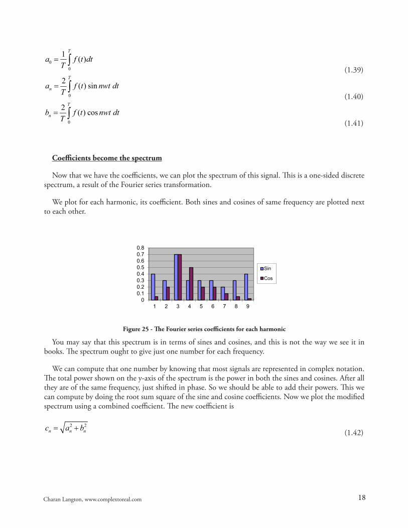
Now that we have the coefficients, we can plot the spectrum of this signal. This is a one-sided discrete spectrum, a result of the Fourier series transformation.
We plot for each harmonic, its coefficient. Both sines and cosines of same frequency are plotted next to each other.
00.10.20.30.40.50.60.70.8
1 2 3 4 5 6 7 8 9
Sin
Cos
Figure 25 - The Fourier series coefficients for each harmonic
You may say that this spectrum is in terms of sines and cosines, and this is not the way we see it in books. The spectrum ought to give just one number for each frequency.
We can compute that one number by knowing that most signals are represented in complex notation. The total power shown on the y-axis of the spectrum is the power in both the sines and cosines. After all they are of the same frequency, just shifted in phase. So we should be able to add their powers. This we can compute by doing the root sum square of the sine and cosine coefficients. Now we plot the modified spectrum using a combined coefficient. The new coefficient is
2 2n n nc a b= + (1.42)
19Charan Langton, www.complextoreal.com
00.2
0.40.6
0.81
1.2
1 2 3 4 5 6 7 8
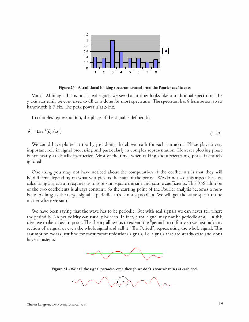
Figure 23 - A traditional looking spectrum created from the Fourier coefficients
Voila! Although this is not a real signal, we see that it now looks like a traditional spectrum. The y-axis can easily be converted to dB as is done for most spectrums. The spectrum has 8 harmonics, so its bandwidth is 7 Hz. The peak power is at 3 Hz.
In complex representation, the phase of the signal is defined by
1tan ( / )n n nb aφ −= (1.42)
We could have plotted it too by just doing the above math for each harmonic. Phase plays a very important role in signal processing and particularly in complex representation. However plotting phase is not nearly as visually instructive. Most of the time, when talking about spectrums, phase is entirely ignored.
One thing you may not have noticed about the computation of the coefficients is that they will be different depending on what you pick as the start of the period. We do not see this aspect because calculating a spectrum requires us to root sum square the sine and cosine coefficients. This RSS addition of the two coefficients is always constant. So the starting point of the Fourier analysis becomes a non-issue. As long as the target signal is periodic, this is not a problem. We will get the same spectrum no matter where we start.
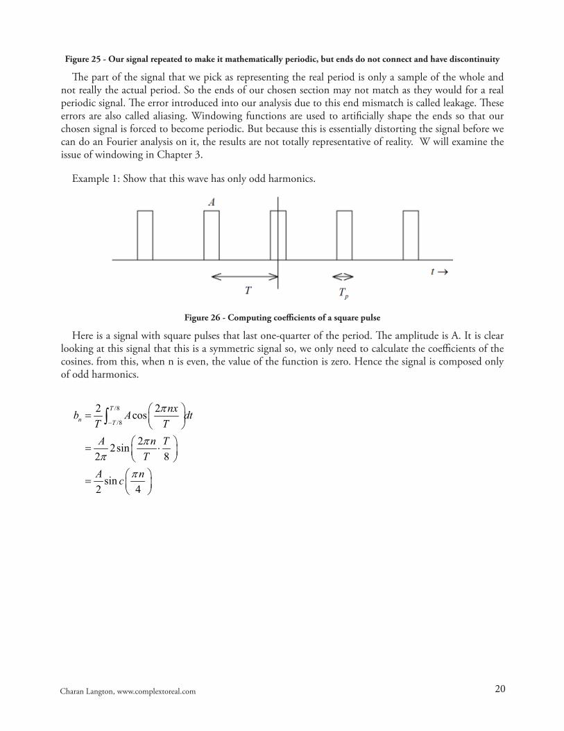
We have been saying that the wave has to be periodic. But with real signals we can never tell where the period is. No periodicity can usually be seen. In fact, a real signal may not be periodic at all. In this case, we make an assumption. The theory allows us to extend the “period” to infinity so we just pick any section of a signal or even the whole signal and call it “The Period”, representing the whole signal. This assumption works just fine for most communications signals, i.e. signals that are steady-state and don’t have transients.
Figure 24 - We call the signal periodic, even though we don’t know what lies at each end.
20Charan Langton, www.complextoreal.com
Figure 25 - Our signal repeated to make it mathematically periodic, but ends do not connect and have discontinuity
The part of the signal that we pick as representing the real period is only a sample of the whole and not really the actual period. So the ends of our chosen section may not match as they would for a real periodic signal. The error introduced into our analysis due to this end mismatch is called leakage. These errors are also called aliasing. Windowing functions are used to artificially shape the ends so that our chosen signal is forced to become periodic. But because this is essentially distorting the signal before we can do an Fourier analysis on it, the results are not totally representative of reality. W will examine the issue of windowing in Chapter 3.
Example 1: Show that this wave has only odd harmonics.
Figure 26 - Computing coefficients of a square pulse
Here is a signal with square pulses that last one-quarter of the period. The amplitude is A. It is clear looking at this signal that this is a symmetric signal so, we only need to calculate the coefficients of the cosines.
from this, when n is even, the value of the function is zero. Hence the signal is composed only of odd harmonics.
/8
/8
2 2cos
22sin2 8
sin2 4
T
n T
nxb A dtT TA n T
TA nc
π
ππ
π
−
=
= ⋅ =
∫
21Charan Langton, www.complextoreal.com
Example 2: Find the coefficients of this wave.
t�®�
T�
A�
Figure 27 - A saw-tooth wave
The wave is odd, so it only has sines.
( )
/2
/2
/22
2 2 2/2
2 2 2sin
2 24 cos sin2 4
2 cos
T
n T
T
T
tA nta dtT T T
A nt T T nttT T n n T
A nn
π
π ππ π
ππ
−
−
=
= − +
= −
∫
such that
0
1
02( 1)n
n
aAanπ
+
=
= −
To be continued....
Copyright 1998, 2012, All rights Reserved Charan Langton

22Charan Langton, www.complextoreal.com

23Charan Langton, www.complextoreal.com