fourier analysis - Åbo akademi |...
TRANSCRIPT
Fourier Analysis
Translation by Olof Staffans of the lecture notes
Fourier analyysi
by
Gustaf Gripenberg
January 5, 2009

0

Contents
0 Integration theory 3
1 Finite Fourier Transform 10
1.1 Introduction . . . . . . . . . . . . . . . . . . . . . . . . . . . . . . 10
1.2 L2-Theory (“Energy theory”) . . . . . . . . . . . . . . . . . . . . 14
1.3 Convolutions (”Faltningar”) . . . . . . . . . . . . . . . . . . . . . 21
1.4 Applications . . . . . . . . . . . . . . . . . . . . . . . . . . . . . . 31
1.4.1 Wirtinger’s Inequality . . . . . . . . . . . . . . . . . . . . 31
1.4.2 Weierstrass Approximation Theorem . . . . . . . . . . . . 32
1.4.3 Solution of Differential Equations . . . . . . . . . . . . . . 33
1.4.4 Solution of Partial Differential Equations . . . . . . . . . . 35
2 Fourier Integrals 36
2.1 L1-Theory . . . . . . . . . . . . . . . . . . . . . . . . . . . . . . . 36
2.2 Rapidly Decaying Test Functions . . . . . . . . . . . . . . . . . . 43
2.3 L2-Theory for Fourier Integrals . . . . . . . . . . . . . . . . . . . 45
2.4 An Inversion Theorem . . . . . . . . . . . . . . . . . . . . . . . . 48
2.5 Applications . . . . . . . . . . . . . . . . . . . . . . . . . . . . . . 52
2.5.1 The Poisson Summation Formula . . . . . . . . . . . . . . 52
2.5.2 Is L1(R) = C0(R) ? . . . . . . . . . . . . . . . . . . . . . . 53
2.5.3 The Euler-MacLauren Summation Formula . . . . . . . . . 54
2.5.4 Schwartz inequality . . . . . . . . . . . . . . . . . . . . . . 55
2.5.5 Heisenberg’s Uncertainty Principle . . . . . . . . . . . . . 55
2.5.6 Weierstrass’ Non-Differentiable Function . . . . . . . . . . 56
2.5.7 Differential Equations . . . . . . . . . . . . . . . . . . . . 59
2.5.8 Heat equation . . . . . . . . . . . . . . . . . . . . . . . . . 63
2.5.9 Wave equation . . . . . . . . . . . . . . . . . . . . . . . . 64
1

CONTENTS 2
3 Fourier Transforms of Distributions 67
3.1 What is a Measure? . . . . . . . . . . . . . . . . . . . . . . . . . . 67
3.2 What is a Distribution? . . . . . . . . . . . . . . . . . . . . . . . 69
3.3 How to Interpret a Function as a Distribution? . . . . . . . . . . . 71
3.4 Calculus with Distributions . . . . . . . . . . . . . . . . . . . . . 73
3.5 The Fourier Transform of a Distribution . . . . . . . . . . . . . . 76
3.6 The Fourier Transform of a Derivative . . . . . . . . . . . . . . . 77
3.7 Convolutions (”Faltningar”) . . . . . . . . . . . . . . . . . . . . . 79
3.8 Convergence in S ′ . . . . . . . . . . . . . . . . . . . . . . . . . . . 85
3.9 Distribution Solutions of ODE:s . . . . . . . . . . . . . . . . . . . 87
3.10 The Support and Spectrum of a Distribution . . . . . . . . . . . . 89
3.11 Trigonometric Polynomials . . . . . . . . . . . . . . . . . . . . . . 93
3.12 Singular differential equations . . . . . . . . . . . . . . . . . . . . 95
4 Fourier Series 99
5 The Discrete Fourier Transform 102
5.1 Definitions . . . . . . . . . . . . . . . . . . . . . . . . . . . . . . . 102
5.2 FFT=the Fast Fourier Transform . . . . . . . . . . . . . . . . . . 104
5.3 Computation of the Fourier Coefficients of a Periodic Function . . 107
5.4 Trigonometric Interpolation . . . . . . . . . . . . . . . . . . . . . 113
5.5 Generating Functions . . . . . . . . . . . . . . . . . . . . . . . . . 115
5.6 One-Sided Sequences . . . . . . . . . . . . . . . . . . . . . . . . . 116
5.7 The Polynomial Interpretation of a Finite Sequence . . . . . . . . 118
5.8 Formal Power Series and Analytic Functions . . . . . . . . . . . . 119
5.9 Inversion of (Formal) Power Series . . . . . . . . . . . . . . . . . . 121
5.10 Multidimensional FFT . . . . . . . . . . . . . . . . . . . . . . . . 122
6 The Laplace Transform 124
6.1 General Remarks . . . . . . . . . . . . . . . . . . . . . . . . . . . 124
6.2 The Standard Laplace Transform . . . . . . . . . . . . . . . . . . 125
6.3 The Connection with the Fourier Transform . . . . . . . . . . . . 126
6.4 The Laplace Transform of a Distribution . . . . . . . . . . . . . . 129
6.5 Discrete Time: Z-transform . . . . . . . . . . . . . . . . . . . . . 130
6.6 Using Laguerra Functions and FFT to Compute Laplace Transforms131
Chapter 0
Integration theory
This is a short summary of Lebesgue integration theory, which will be used in
the course.
Fact 0.1. Some subsets (=“delmangder”) E ⊂ R = (−∞,∞) are “measurable”
(=“matbara”) in the Lebesgue sense, others are not.
General Assumption 0.2. All the subsets E which we shall encounter in this
course are measurable.
Fact 0.3. All measurable subsets E ⊂ R have a measure (=“matt”) m(E), which
in simple cases correspond to “ the total length” of the set. E.g., the measure of
the interval (a, b) is b− a (and so is the measure of [a, b] and [a, b)).
Fact 0.4. Some sets E have measure zero, i.e., m(E) = 0. True for example if
E consists of finitely many (or countably many) points. (“mattet noll”)
The expression a.e. = “almost everywhere” (n.o. = nastan overallt) means that
something is true for all x ∈ R, except for those x which belong to some set E
with measure zero. For example, the function
f(x) =
1, |x| ≤ 1
0, |x| > 1
is continuous almost everywhere. The expression fn(x) → f(x) a.e. means that
the measure of the set x ∈ R for which fn(x) 9 f(x) is zero.
Think: “In all but finitely many points” (this is a simplification).
3

CHAPTER 0. INTEGRATION THEORY 4
Notation 0.5. R = (−∞,∞), C = complex plane.
The set of Riemann integrable functions f : I 7→ C (I ⊆ R is an interval) such
that ∫
I
|f(x)|pdx <∞, 1 ≤ p <∞,
though much larger than the space C(I) of continuous functions on I, is not
big enough for our purposes. This defect can be remedied by the use of the
Lebesgue integral instead of the Riemann integral. The Lebesgue integral is
more complicated to define and develop than the Riemann integral, but as a tool
it is easier to use as it has better properties. The main difference between the
Riemann and the Lebesgue integral is that the former uses intervals and their
lengths while the latter uses more general point sets and their measures.
Definition 0.6. A function f : I 7→ C (I ∈ R is an interval) is measurable if
there exists a sequence of continuous functions fn so that
fn(x) → f(x) for almost all x ∈ I
(i.e., the set of points x ∈ I for which fn(x) 9 f(x) has measure zero).
General Assumption 0.7. All the functions that we shall encounter in this
course are measurable.
Thus, the word “measurable” is understood throughout (when needed).
Definition 0.8. Let 1 ≤ p < ∞, and I ⊂ R an interval. We write f ∈ Lp(I) if
(f is measurable and) ∫
I
|f(x)|pdx <∞.
We define the norm of f in Lp(I) to be
‖f‖Lp(I) =
(∫
I
|f(x)|pdx)1/p
.
Physical interpretation:
p = 1 ‖f‖L1(I) =
∫
I
|f(x)|dx
CHAPTER 0. INTEGRATION THEORY 5
= “the total mass”. “Probability density” if f(x) ≥ 0, or a “size of the total
population”.
p = 2 ‖f‖L2(I) =
(∫
I
|f(x)|2dx)1/2
= “total energy” (e.g. in an electrical signal, such as alternating current).
These two cases are the two important ones (we ignore the rest). The third
important case is p = ∞.
Definition 0.9. f ∈ L∞(I) if (f is measurable and) there exists a number
M <∞ such that
|f(x)| < M a.e.
The norm of f is
‖f‖L∞(I) = infM : |f(x)| ≤M a.e.,
and it is denoted by
‖f‖L∞(I) = ess supx∈I
|f(x)|
(“essential supremum”, ”vasentligt supremum”).
Think: ‖f‖L∞(I) = “the largest value of f in I if we ignore a set of measure
zero”. For example:
f(x) =
0, x < 0
2, x = 0
1, x > 0
⇒ ‖f‖L∞(I) = 1.
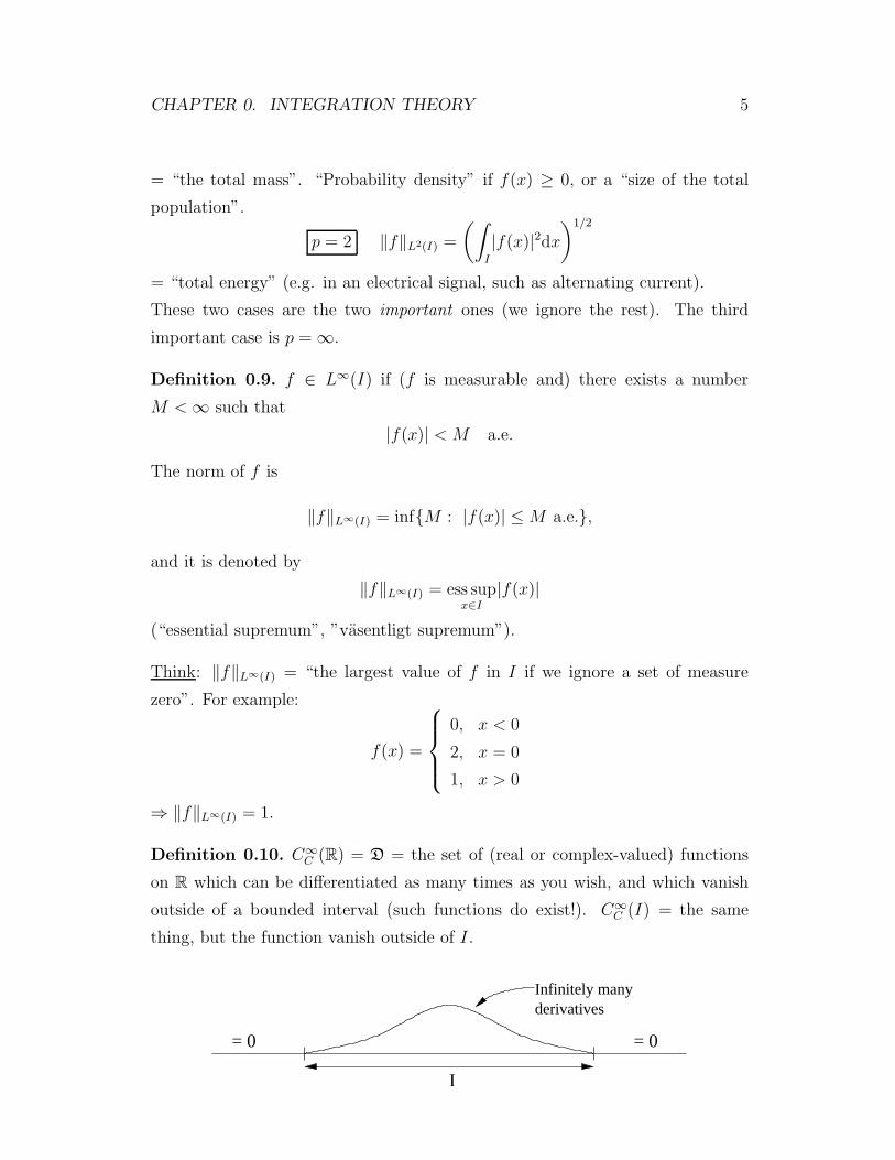
Definition 0.10. C∞C (R) = D = the set of (real or complex-valued) functions
on R which can be differentiated as many times as you wish, and which vanish
outside of a bounded interval (such functions do exist!). C∞C (I) = the same
thing, but the function vanish outside of I.
I
= 0 = 0
Infinitely manyderivatives
CHAPTER 0. INTEGRATION THEORY 6
Theorem 0.11. Let I ⊂ R be an interval. Then C∞C (I) is dense in Lp(I) for
all p, 1 ≤ p < ∞ (but not in L∞(I)). That is, for every f ∈ Lp(I) it is possible
to find a sequence fn ∈ C∞C (I) so that
limn→∞
‖fn − f‖Lp(I) = 0.
Proof. “Straightforward” (but takes a lot of work).
Theorem 0.12 (Fatou’s lemma). Let fn(x) ≥ 0 and let fn(x) → f(x) a.e. as
n→ ∞. Then ∫
I
f(x)dx ≤ limn→∞
∫
I
fn(x)dx
(if the latter limit exists). Thus,∫
I
[limn→∞
fn(x)]dx ≤ lim
n→∞
∫
I
fn(x)dx
if fn ≥ 0 (“f can have no more total mass than fn, but it may have less”). Often
we have equality, but not always.
Ex.
fn(x) =
n, 0 ≤ x ≤ 1/n
0, otherwise.
Homework: Compute the limits above in this case.
Theorem 0.13 (Monotone Convergence Theorem). If
0 ≤ f1(x) ≤ f2(x) ≤ . . .
and fn(x) → f(x) a.e., then∫
I
f(x)dx = limn→∞
∫
I
fn(x)dx (≤ ∞).
Thus, for a positive increasing sequence we have∫
I
[limn→∞
fn(x)]dx = lim
n→∞
∫
I
fn(x)dx
(the mass of the limit is the limit of the masses).
Theorem 0.14 (Lebesgue’s dominated convergence theorem). (Extremely use-
ful)
If fn(x) → f(x) a.e. and |fn(x)| ≤ g(x) a.e. and∫
I
g(x)dx <∞ (i.e., g ∈ L1(I)),
CHAPTER 0. INTEGRATION THEORY 7
then ∫
I
f(x)dx =
∫
I
[limn→∞
fn(x)]dx = lim
n→∞
∫
I
fn(x)dx.
Theorem 0.15 (Fubini’s theorem). (Very useful for multiple integrals).
If f (is measurable and)∫
I
∫
J
|f(x, y)|dy dx <∞
then the double integral ∫∫
I×Jf(x, y)dy dx
is well-defined, and equal to
=
∫
x∈I
(∫
y∈Jf(x, y)dy
)dx
=
∫
y∈J
(∫
x∈If(x, y)dx
)dy
If f ≥ 0, then all three integrals are well-defined, possibly = ∞, and if one of
them is <∞, then so are the others, and they are equal.
Note: These theorems are very useful, and often easier to use than the corre-
sponding theorems based on the Rieman integral.
Theorem 0.16 (Integration by parts a la Lebesgue). Let [a, b]be a finite interval,
u ∈ L1([a, b]), v ∈ L1([a, b]),
U(t) = U(a) +
∫ t
a
u(s)ds, V (t) = V (a) +
∫ t
a
v(s)ds, t ∈ [a, b].
Then ∫ b
a
u(t)V (t)dt = [U(t)V (t)]ba −∫ b
a
U(t)v(t)dt.
Proof.∫ b
a
u(t)V (t) =
∫ b
a
u(t)
∫ t
a
v(s)dsdt
Fubini=
(U(b) − U(a)
)V (a) +
∫ b
a
(∫ b
s
u(t)dt
)v(s)ds.
Since∫ b
s
u(t)dt =(∫ b
a
−∫ s
a
)u(t)dt = U(b) − U(a) −
∫ s
a
u(t)dt = U(b) − U(s),
CHAPTER 0. INTEGRATION THEORY 8
we get∫ b
a
u(t)V (t)dt =(U(b) − U(a)
)V (a) +
∫ b
a
(U(b) − U(s)) v(s)ds
=(U(b) − U(a)
)V (a) + U(b)
(V (b) − V (a)
)−∫ b
a
U(s)v(s)ds
= U(b)V (b) − U(a)V (a) −∫ b
a
U(s)v(s)ds.
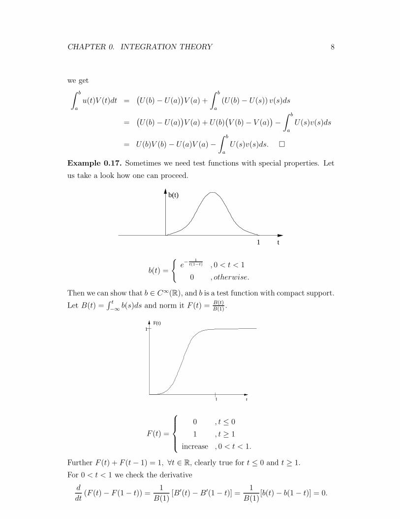
Example 0.17. Sometimes we need test functions with special properties. Let
us take a look how one can proceed.
1 t
b(t)
b(t) =
e−
1t(1−t) , 0 < t < 1
0 , otherwise.
Then we can show that b ∈ C∞(R), and b is a test function with compact support.
Let B(t) =∫ t−∞ b(s)ds and norm it F (t) = B(t)
B(1).
1
1F(t)
t
F (t) =
0 , t ≤ 0
1 , t ≥ 1
increase , 0 < t < 1.
Further F (t) + F (t− 1) = 1, ∀t ∈ R, clearly true for t ≤ 0 and t ≥ 1.
For 0 < t < 1 we check the derivative
d
dt(F (t) − F (1 − t)) =
1
B(1)[B′(t) − B′(1 − t)] =
1
B(1)[b(t) − b(1 − t)] = 0.

CHAPTER 0. INTEGRATION THEORY 9
F(t)F(1−t)
Let G(t) = F (Nt). Then G increases from 0 to 1 on the interval 0 ≤ t ≤ 1N
.
G(t) +G(1
N− t) = F (Nt) − F (1 −Nt) = 1, ∀t ∈ R.
1/N 1
G(t)G(1/N−t)

Chapter 1
The Fourier Series of a Periodic
Function
1.1 Introduction
Notation 1.1. We use the letter T with a double meaning:
a) T = [0, 1)
b) In the notations Lp(T), C(T), Cn(T) and C∞(T) we use the letter T to
imply that the functions are periodic with period 1, i.e., f(t + 1) = f(t)
for all t ∈ R. In particular, in the continuous case we require f(1) = f(0).
Since the functions are periodic we know the whole function as soon as we
know the values for t ∈ [0, 1).
Notation 1.2. ‖f‖Lp(T) =(∫ 1
0|f(t)|pdt
)1/p
, 1 ≤ p <∞. ‖f‖C(T) = maxt∈T |f(t)|(f continuous).
Definition 1.3. f ∈ L1(T) has the Fourier coefficients
f(n) =
∫ 1
0
e−2πintf(t)dt, n ∈ Z,
where Z = 0,±1,±2, . . .. The sequence f(n)n∈Z is the (finite) Fourier
transform of f .
Note:
f(n) =
∫ s+1
s
e−2πintf(t)dt ∀s ∈ R,
10
CHAPTER 1. FINITE FOURIER TRANSFORM 11
since the function inside the integral is periodic with period 1.
Note: The Fourier transform of a periodic function is a discrete sequence.
Theorem 1.4.
i) |f(n)| ≤ ‖f‖L1(T), ∀n ∈ Z
ii) limn→±∞ f(n) = 0.
Note: ii) is called the Riemann–Lebesgue lemma.
Proof.
i) |f(n)| = |∫ 1
0e−2πintf(t)dt| ≤
∫ 1
0|e−2πintf(t)|dt =
∫ 1
0|f(t)|dt = ‖f‖L1(T) (by
the triangle inequality for integrals).
ii) First consider the case where f is continuously differentiable, with f(0) = f(1).
Then integration by parts gives
f(n) =
∫ 1
0
e−2πintf(t)dt
=1
−2πin
[e−2πintf(t)
]10+
1
2πin
∫ 1
0
e−2πintf ′(t)dt
= 0 +1
2πinf ′(n), so by i),
|f(n)| =1
2πn|f ′(n)| ≤ 1
2πn
∫ 1
0
|f ′(s)|ds→ 0 as n→ ∞.
In the general case, take f ∈ L1(T) and ε > 0. By Theorem 0.11 we can
choose some g which is continuously differentiable with g(0) = g(1) = 0 so
that
‖f − g‖L1(T) =
∫ 1
0
|f(t) − g(t)|dt ≤ ε/2.
By i),
|f(n)| = |f(n) − g(n) + g(n)|≤ |f(n) − g(n)| + |g(n)|≤ ‖f − g‖L1(T) + |g(n)|≤ ǫ/2 + |g(n)|.
By the first part of the proof, for n large enough, |g(n)| ≤ ε/2, and so
|f(n)| ≤ ε.
This shows that |f(n)| → 0 as n→ ∞.
CHAPTER 1. FINITE FOURIER TRANSFORM 12
Question 1.5. If we know f(n)∞n=−∞ then can we reconstruct f(t)?
Answer: is more or less ”Yes”.
Definition 1.6. Cn(T) = n times continuously differentiable functions, periodic
with period 1. (In particular, f (k)(1) = f (k)(0) for 0 ≤ k ≤ n.)
Theorem 1.7. For all f ∈ C1(T) we have
f(t) = limN→∞M→∞
N∑
n=−Mf(n)e2πint, t ∈ R. (1.1)
We shall see later that the convergence is actually uniform in t.
Proof. Step 1. We shift the argument of f by replacing f(s) by g(s) = f(s+t).
Then
g(n) = e2πintf(n),
and (1.1) becomes
f(t) = g(0) = limN→∞M→∞
N∑
n=−Mf(n)e2πint.
Thus, it suffices to prove the case where t = 0 .
Step 2: If g(s) is the constant function g(s) ≡ g(0) = f(t), then (1.1) holds since
g(0) = g(0) and g(n) = 0 for n 6= 0 in this case. Replace g(s) by
h(s) = g(s) − g(0).
Then h satisfies all the assumptions which g does, and in addition, h(0) = 0.
Thus it suffices to prove the case where both t = 0 and f(0) = 0. For simplicity
we write f instead of h, but we suppose below that t = 0 and f(0) = 0
Step 2: Define
g(s) =
f(s)
e−2πis−1, s 6= integer (=“heltal”)
if ′(0)2π
, s = integer.
For s = n = integer we have e−2πis − 1 = 0, and by l’Hospital’s rule
lims→n
g(s) = lims→0
f ′(s)
−2πie−2πis=f ′(s)
−2πi= g(n)
CHAPTER 1. FINITE FOURIER TRANSFORM 13
(since e−i2πn = 1). Thus g is continuous. We clearly have
f(s) =(e−2πis − 1
)g(s), (1.2)
so
f(n) =
∫
T
e−2πinsf(s)ds (use (1.2))
=
∫
T
e−2πins(e−2πis − 1)g(s)ds
=
∫
T
e−2πi(n+1)sg(s)ds−∫
T
e−2πinsg(s)ds
= g(n+ 1) − g(n).
Thus,N∑
n=−Mf(n) = g(N + 1) − g(−M) → 0
by the Rieman–Lebesgue lemma (Theorem 1.4)
By working a little bit harder we get the following stronger version of Theorem
1.7:
Theorem 1.8. Let f ∈ L1(T), t0 ∈ R, and suppose that
∫ t0+1
t0−1
∣∣∣f(t) − f(t0)
t− t0
∣∣∣dt <∞. (1.3)
Then
f(t0) = limN→∞M→∞
N∑
n=−Mf(n)e2πint0 t ∈ R
Proof. We can repeat Steps 1 and 2 of the preceding proof to reduce the The-
orem to the case where t0 = 0 and f(t0) = 0. In Step 3 we define the function
g in the same way as before for s 6= n, but leave g(s) undefined for s = n.
Since lims→0 s−1(e−2πis − 1) = −2πi 6= 0, the function g belongs to L1(T) if and
only if condition (1.3) holds. The continuity of g was used only to ensure that
g ∈ L1(T), and since g ∈ L1(T) already under the weaker assumption (1.3), the
rest of the proof remains valid without any further changes.
CHAPTER 1. FINITE FOURIER TRANSFORM 14
Summary 1.9. If f ∈ L1(T), then the Fourier transform f(n)∞n=−∞ of f is
well-defined, and f(n) → 0 as n → ∞. If f ∈ C1(T), then we can reconstruct f
from its Fourier transform through
f(t) =
∞∑
n=−∞f(n)e2πint
(= lim
N→∞M→∞
N∑
n=−Mf(n)e2πint
).
The same reconstruction formula remains valid under the weaker assumption of
Theorem 1.8.
1.2 L2-Theory (“Energy theory”)
This theory is based on the fact that we can define an inner product (scalar
product) in L2(T), namely
〈f, g〉 =
∫ 1
0
f(t)g(t)dt, f, g ∈ L2(T).
Scalar product means that for all f, g, h ∈ L2(T)
i) 〈f + g, h〉 = 〈f, h〉 + 〈g, h〉
ii) 〈λf, g〉 = λ〈f, g〉 ∀λ ∈ C
iii) 〈g, f〉 = 〈f, g〉 (complex conjugation)
iv) 〈f, f〉 ≥ 0, and = 0 only when f ≡ 0.
These are the same rules that we know from the scalar products in Cn. In
addition we have
‖f‖2L2(T) =
∫
T
|f(t)|2dt =
∫
T
f(t)f(t)dt = 〈f, f〉.
This result can also be used to define the Fourier transform of a function f ∈L2(T), since L2(T) ⊂ L1(T).
Lemma 1.10. Every function f ∈ L2(T) also belongs to L1(T), and
‖f‖L1(T) ≤ ‖f‖L2(T).

CHAPTER 1. FINITE FOURIER TRANSFORM 15
Proof. Interpret∫
T|f(t)|dt as the inner product of |f(t)| and g(t) ≡ 1. By
Schwartz inequality (see course on Analysis II),
|〈f, g〉| =∫
T
|f(t)| · 1dt ≤ ‖f‖L2 · ‖g‖L2 = ‖f‖L2(T)
∫
T
12dt = ‖f‖L2(T).
Thus, ‖f‖L1(T) ≤ ‖f‖L2(T). Therefore:
f ∈ L2(t) =⇒∫
T
|f(t)|dt <∞
=⇒ f(n) =
∫
T
e−2πintf(t)dt is defined for all n.
It is not true that L2(R) ⊂ L1(R). Counter example:
f(t) =1√
1 + t2
∈ L2(R)
/∈ L1(R)
∈ C∞(R)
(too large at ∞).
Notation 1.11. en(t) = e2πint, n ∈ Z, t ∈ R.
Theorem 1.12 (Plancherel’s Theorem). Let f ∈ L2(T). Then
i)∑∞
n=−∞|f(n)|2 =∫ 1
0|f(t)|2dt = ‖f‖2
L2(T),
ii) f =∑∞
n=−∞ f(n)en in L2(T) (see explanation below).
Note: This is a very central result in, e.g., signal processing.
Note: It follows from i) that the sum∑∞
n=−∞|f(n)|2 always converges if f ∈ L2(T)
Note: i) says that
∞∑
n=−∞|f(n)|2 = the square of the total energy of the Fourier coefficients
= the square of the total energy of the original signal f
=
∫
T
|f(t)|2dt
Note: Interpretation of ii): Define
fM,N =
N∑
n=−Mf(n)en =
N∑
n=−Mf(n)e2πint.
CHAPTER 1. FINITE FOURIER TRANSFORM 16
Then
limM→∞N→∞
‖f − fM,N‖2 = 0 ⇐⇒
limM→∞N→∞
∫ 1
0
|f(t) − fM,N(t)|2dt = 0
(fM,N(t) need not converge to f(t) at every point, and not even almost every-
where).
The proof of Theorem 1.12 is based on some auxiliary results:
Theorem 1.13. If gn ∈ L2(T), fN =∑N
n=0 gn, gn ⊥ gm, and∑∞
n=0‖gn‖2L2(T) <∞,
then the limit
f = limN→∞
N∑
n=0
gn
exists in L2.
Proof. Course on “Analysis II” and course on “Hilbert Spaces”.
Interpretation: Every orthogonal sum with finite total energy converges.
Lemma 1.14. Suppose that∑∞
n=−∞|c(n)| <∞. Then the series
∞∑
n=−∞c(n)e2πint
converges uniformly to a continuous limit function g(t).
Proof.
i) The series∑∞
n=−∞ c(n)e2πint converges absolutely (since |e2πint| = 1), so
the limit
g(t) =
∞∑
n=−∞c(n)e2πint
exist for all t ∈ R.
ii) The convergens is uniform, because the error
|m∑
n=−mc(n)e2πint − g(t)| = |
∑
|n|>mc(n)e2πint|
≤∑
|n|>m|c(n)e2πint|
=∑
|n|>m|c(n)| → 0 as m→ ∞.
CHAPTER 1. FINITE FOURIER TRANSFORM 17
iii) If a sequence of continuous functions converge uniformly, then the limit is
continuous (proof “Analysis II”).
proof of Theorem 1.12. (Outline)
0 ≤ ‖f − fM,N‖2 = 〈f − fM,N , f − fM,N〉= 〈f, f〉︸ ︷︷ ︸
I
−〈fM,N , f〉︸ ︷︷ ︸II
−〈f, fM,N〉︸ ︷︷ ︸III
+ 〈fM,N , fM,N〉︸ ︷︷ ︸IV
I = 〈f, f〉 = ‖f‖2L2(T).
II = 〈N∑
n=−Mf(n)en, f〉 =
N∑
n=−Mf(n)〈en, f〉
=N∑
n=−Mf(n)〈f, en〉 =
N∑
n=−Mf(n)f(n)
=
N∑
n=−M|f(n)|2.
III = (the complex conjugate of II) = II.
IV =⟨ N∑
n=−Mf(n)en,
N∑
m=−Mf(m)em
⟩
=N∑
n=−Mf(n)f(m) 〈en, em〉︸ ︷︷ ︸
δmn
=N∑
n=−M|f(n)|2 = II = III.
Thus, adding I − II − III + IV = I − II ≥ 0, i.e.,
‖f‖2L2(T) −
N∑
n=−M|f(n)|2 ≥ 0.
This proves Bessel’s inequality
∞∑
n=−∞|f(n)|2 ≤ ‖f‖2
L2(T). (1.4)
How do we get equality?
By Theorem 1.13, applied to the sums
N∑
n=0
f(n)en and
−1∑
n=−Mf(n)en,

CHAPTER 1. FINITE FOURIER TRANSFORM 18
the limit
g = limM→∞N→∞
fM,N = limM→∞N→∞
N∑
n=−Mf(n)en (1.5)
does exist. Why is f = g? (This means that the sequence en is complete!). This
is (in principle) done in the following way
i) Argue as in the proof of Theorem 1.4 to show that if f ∈ C2(T), then
|f(n)| ≤ 1/(2πn)2‖f ′′‖L1 for n 6= 0. In particular, this means that∑∞
n=−∞|f(n)| < ∞. By Lemma 1.14, the convergence in (1.5) is actually
uniform, and by Theorem 1.7, the limit is equal to f . Uniform convergence
implies convergence in L2(T), so even if we interpret (1.5) in the L2-sense,
the limit is still equal to f a.e. This proves that fM,N → f in L2(T) if
f ∈ C2(T).
ii) Approximate an arbitrary f ∈ L2(T) by a function h ∈ C2(T) so that
‖f − h‖L2(T) ≤ ε.
iii) Use i) and ii) to show that ‖f − g‖L2(T) ≤ ε, where g is the limit in (1.5).
Since ε is arbitrary, we must have g = f .
Definition 1.15. Let 1 ≤ p <∞.
ℓp(Z) = set of all sequences an∞n=−∞ satisfying∞∑
n=−∞|an|p <∞.
The norm of a sequence a ∈ ℓp(Z) is
‖a‖ℓp(Z) =
( ∞∑
n=−∞|an|p
)1/p
Analogous to Lp(I):
p = 1 ‖a‖ℓ1(Z) = ”total mass” (probability),
p = 2 ‖a‖ℓ2(Z) = ”total energy”.
In the case of p = 2 we also define an inner product
〈a, b〉 =
∞∑
n=−∞anbn.

CHAPTER 1. FINITE FOURIER TRANSFORM 19
Definition 1.16. ℓ∞(Z) = set of all bounded sequences an∞n=−∞. The norm
in ℓ∞(Z) is
‖a‖ℓ∞(Z) = supn∈Z
|an|.
For details: See course in ”Analysis II”.
Definition 1.17. c0(Z) = the set of all sequences an∞n=−∞ satisfying limn→±∞ an = 0.
We use the norm
‖a‖c0(Z) = maxn∈Z
|an|
in c0(Z).
Note that c0(Z) ⊂ ℓ∞(Z), and that
‖a‖c0(Z) = ‖a‖ℓ∞(Z)
if a∞n=−∞ ∈ c0(Z).
Theorem 1.18. The Fourier transform maps L2(T) one to one onto ℓ2(Z), and
the Fourier inversion formula (see Theorem 1.12 ii) maps ℓ2(Z) one to one onto
L2(T). These two transforms preserves all distances and scalar products.
Proof. (Outline)
i) If f ∈ L2(T) then f ∈ ℓ2(Z). This follows from Theorem 1.12.
ii) If an∞n=−∞ ∈ ℓ2(Z), then the series
N∑
n=−Mane
2πint
converges to some limit function f ∈ L2(T). This follows from Theorem
1.13.
iii) If we compute the Fourier coefficients of f , then we find that an = f(n).
Thus, an∞n=−∞ is the Fourier transform of f . This shows that the Fourier
transform maps L2(T) onto ℓ2(Z).
iv) Distances are preserved. If f ∈ L2(T), g ∈ L2(T), then by Theorem 1.12
i),
‖f − g‖L2(T) = ‖f(n) − g(n)‖ℓ2(Z),
i.e., ∫
T
|f(t) − g(t)|2dt =
∞∑
n=−∞|f(n) − g(n)|2.

CHAPTER 1. FINITE FOURIER TRANSFORM 20
v) Inner products are preserved:
∫
T
|f(t) − g(t)|2dt = 〈f − g, f − g〉
= 〈f, f〉 − 〈f, g〉 − 〈g, f〉 + 〈g, g〉= 〈f, f〉 − 〈f, g〉 − 〈f, g〉 + 〈g, g〉= 〈f, f〉 + 〈g, g〉 − 2ℜRe〈f, g〉.
In the same way,
∞∑
n=−∞|f(n) − g(n)|2 = 〈f − g, f − g〉
= 〈f , f〉 + 〈g, g〉 − 2ℜ〈f , g〉.
By iv), subtracting these two equations from each other we get
ℜ〈f, g〉 = ℜ〈f , g〉.
If we replace f by if , then
Im〈f, g〉 = Re i〈f, g〉 = ℜ〈if, g〉= ℜ〈if , g〉 = Re i〈f , g〉= Im〈f , g〉.
Thus, 〈f, g〉L2(R) = 〈f , g〉ℓ2(Z), or more explicitely,
∫
T
f(t)g(t)dt =
∞∑
n=−∞f(n)g(n). (1.6)
This is called Parseval’s identity.
Theorem 1.19. The Fourier transform maps L1(T) into c0(Z) (but not onto),
and it is a contraction, i.e., the norm of the image is ≤ the norm of the original
function.
Proof. This is a rewritten version of Theorem 1.4. Parts i) and ii) say that
f(n)∞n=−∞ ∈ c0(Z), and part i) says that ‖f(n)‖c0(Z) ≤ ‖f‖L1(T).
The proof that there exist sequences in c0(Z) which are not the Fourier transform
of some function f ∈ L1(T) is much more complicated.
CHAPTER 1. FINITE FOURIER TRANSFORM 21
1.3 Convolutions (”Faltningar”)
Definition 1.20. The convolution (”faltningen”) of two functions f, g ∈ L1(T)
is
(f ∗ g)(t) =
∫
T
f(t− s)g(s)ds,
where∫
T=∫ α+1
αfor all α ∈ R, since the function s 7→ f(t− s)g(s) is periodic.
Note: In this integral we need values of f and g outside of the interval [0, 1), and
therefore the periodicity of f and g is important.
Theorem 1.21. If f, g ∈ L1(T), then (f ∗ g)(t) is defined almost everywhere,
and f ∗ g ∈ L1(T). Furthermore,
∥∥f ∗ g∥∥L1(T)
≤∥∥f∥∥L1(T)
∥∥g∥∥L1(T)
(1.7)
Proof. (We ignore measurability)
We begin with (1.7)
∥∥f ∗ g∥∥L1(T)
=
∫
T
|(f ∗ g)(t)| dt
=
∫
T
∣∣∫
T
f(t− s)g(s) ds∣∣ dt
-ineq.
≤∫
t∈T
∫
s∈T|f(t− s)g(s)| ds dt
Fubini=
∫
s∈T
(∫
t∈T|f(t− s)| dt
)|g(s)| ds
Put v=t−s,dv=dt=
∫
s∈T
(∫
v∈T|f(v)| dv
)
︸ ︷︷ ︸=‖f‖L1(T)
|g(s)| ds
= ‖f‖L1(T)
∫
s∈T|g(s)| ds = ‖f‖L1(T)‖g‖L1(T)
This integral is finite. By Fubini’s Theorem 0.15∫
T
f(t− s)g(s)ds
is defined for almost all t.
Theorem 1.22. For all f, g ∈ L1(T) we have
(f ∗ g)(n) = f(n)g(n), n ∈ Z

CHAPTER 1. FINITE FOURIER TRANSFORM 22
Proof. Homework.
Thus, the Fourier transform maps convolution onto pointwise multiplication.
Theorem 1.23. If k ∈ Cn(T) (n times continuously differentiable) and f ∈ L1(T),
then k ∗ f ∈ Cn(T), and (k ∗ f)(m)(t) = (k(m) ∗ f)(t) for all m = 0, 1, 2, . . . , n.
Proof. (Outline) We have for all h > 0
1
h[(k ∗ f) (t+ h) − (k ∗ f)(t)] =
1
h
∫ 1
0
[k(t+ h− s) − k(t− s)] f(s)ds.
By the mean value theorem,
k(t+ h− s) = k(t− s) + hk′(ξ),
for some ξ ∈ [t−s, t−s+h], and 1h[k(t+h−s)−k(t−s)] = f(ξ) → k′(t−s) as
h→ 0, and∣∣ 1h[k(t+h−s)−k(t−s)]
∣∣ = |f ′(ξ)| ≤M, where M = supT |k′(s)|. By
the Lebesgue dominated convergence theorem (which is true also if we replace
n→ ∞ by h→ 0)(take g(x) = M |f(x)|)
limh→0
∫ 1
0
1
h[k(t+ h− s) − k(t− s)]f(s) ds =
∫ 1
0
k′(t− s)f(s) ds,
so k ∗ f is differentiable, and (k ∗ f)′ = k′ ∗ f . By repeating this n times we find
that k ∗ f is n times differentiable, and that (k ∗ f)(n) = k(n) ∗ f . We must still
show that k(n) ∗ f is continuous. This follows from the next lemma.
Lemma 1.24. If k ∈ C(T) and f ∈ L1(T), then k ∗ f ∈ C(T).
Proof. By Lebesgue dominated convergence theorem (take g(t) = 2‖k‖C(T)f(t)),
(k ∗ f)(t+ h) − (k ∗ f)(t) =
∫ 1
0
[k(t+ h− s) − k(t− s)]f(s)ds→ 0 as h→ 0.
Corollary 1.25. If k ∈ C1(T) and f ∈ L1(T), then for all t ∈ R
(k ∗ f)(t) =
∞∑
n=−∞e2πintk(n)f(n).
Proof. Combine Theorems 1.7, 1.22 and 1.23.
Interpretation: This is a generalised inversion formula. If we choose k(n) so
that
CHAPTER 1. FINITE FOURIER TRANSFORM 23
i) k(n) ≈ 1 for small |n|
ii) k(n) ≈ 0 for large |n|,
then we set a “filtered” approximation of f , where the “high frequences” (= high
values of |n|) have been damped but the “low frequences” (= low values of |n|)remain. If we can take k(n) = 1 for all n then this gives us back f itself, but this
is impossible because of the Riemann-Lebesgue lemma.
Problem: Find a “good” function k ∈ C1(T) of this type.
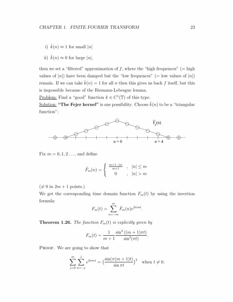
Solution: “The Fejer kernel” is one possibility. Choose k(n) to be a “triangular
function”:
n = 0 n = 4
F (n)4
Fix m = 0, 1, 2 . . . , and define
Fm(n) =
m+1−|n|m+1
, |n| ≤ m
0 , |n| > m
( 6= 0 in 2m+ 1 points.)
We get the corresponding time domain function Fm(t) by using the invertion
formula:
Fm(t) =
m∑
n=−mFm(n)e2πint.
Theorem 1.26. The function Fm(t) is explicitly given by
Fm(t) =1
m+ 1
sin2 ((m+ 1)πt)
sin2(πt).
Proof. We are going to show that
m∑
j=0
j∑
n=−je2πint =
(sin(π(m+ 1)t)
sin πt
)2when t 6= 0.
CHAPTER 1. FINITE FOURIER TRANSFORM 24
Let z = e2πit, z = e−2πit, for t 6= n, n = 0, 1, 2, . . . . Also z 6= 1, and
j∑
n=−je2πint =
j∑
n=0
e2πint +
j∑
n=1
e−2πint =
j∑
n=0
zn +
j∑
n=1
zn
=1 − zj+1
1 − z+z(1 − zj)
1 − z=
1 − zj+1
1 − z+
=1︷︸︸︷z · z(1 − zj)
z − z · z︸︷︷︸=1
=zj − zj+1
1 − z.
Hence
m∑
j=0
j∑
n=−je2πint =
m∑
j=0
zj − zj+1
1 − z=
1
1 − z
(m∑
j=0
zj −m∑
j=0
zj+1
)
=1
1 − z
(1 − zm+1
1 − z− z
(1 − zm+1
1 − z
))
=1
1 − z
[1 − zm+1
1 − z−
=1︷︸︸︷z · z(1 − zm+1
z(1 − z)
]
=1
1 − z
[1 − zm+1
1 − z− 1 − zm+1
z − 1
]
=−zm+1 + 2 − zm+1
|1 − z|2 .
sin t = 12i
(eit − e−it), cos t = 12(eit + e−it). Now
|1 − z| = |1 − e2πit| = |eiπt(e−iπt − eiπt)| = |e−iπt − eiπt| = 2|sin(πt)|
and
zm+1 − 2 + zm+1 = e2πi(m+1) − 2 + e−2πi(m+1)
=(eπi(m+1) − e−πi(m+1)
)2=(2i sin(π(m+ 1))
)2.
Hencem∑
j=0
j∑
n=−je2πint =
4(sin(π(m+ 1)))2
4(sin(πt))2=(sin(π(m+ 1))
sin(πt)
)2
Note also that
m∑
j=0
j∑
n=−je2πint =
m∑
n=−m
m∑
j=|n|e2πint =
m∑
n=−m(m+ 1 − |n|)e2πint.

CHAPTER 1. FINITE FOURIER TRANSFORM 25
-2 -1 1 2
1
2
3
4
5
6
Comment 1.27.
i) Fm(t) ∈ C∞(T) (infinitely many derivatives).
ii) Fm(t) ≥ 0.
iii)∫
T|Fm(t)|dt =
∫TFm(t)dt = Fm(0) = 1,
so the total mass of Fm is 1.
iv) For all δ, 0 < δ < 12,
limm→∞
∫ 1−δ
δ
Fm(t)dt = 0,
i.e. the mass of Fm gets concentrated to the integers t = 0,±1,±2 . . .
as m→ ∞.
Definition 1.28. A sequence of functions Fm with the properties i)-iv) above is
called a (periodic) approximate identity. (Often i) is replaced by Fm ∈ L1(T).)
Theorem 1.29. If f ∈ L1(T), then, as m→ ∞,
i) Fm ∗ f → f in L1(T), and
ii) (Fm ∗ f)(t) → f(t) for almost all t.
Here i) means that∫
T|(Fm ∗ f)(t) − f(t)|dt→ 0 as m→ ∞
Proof. See page 27.
By combining Theorem 1.23 and Comment 1.27 we find that Fm ∗ f ∈ C∞(T).
This combined with Theorem 1.29 gives us the following periodic version of
Theorem 0.11:

CHAPTER 1. FINITE FOURIER TRANSFORM 26
Corollary 1.30. For every f ∈ L1(T) and ε > 0 there is a function g ∈ C∞(T)
such that ‖g − f‖L1(T) ≤ ε.
Proof. Choose g = Fm ∗ f where m is large enough.
To prove Theorem 1.29 we need a number of simpler results:
Lemma 1.31. For all f, g ∈ L1(T) we have f ∗ g = g ∗ f
Proof.
(f ∗ g)(t) =
∫
T
f(t− s)g(s)ds
t−s=v,ds=−dv=
∫
T
f(v)g(t− v)dv = (g ∗ f)(t)
We also need:
Theorem 1.32. If g ∈ C(T), then Fm ∗ g → g uniformly as m→ ∞, i.e.
maxt∈R
|(Fm ∗ g)(t) − g(t)| → 0 as m→ ∞.
Proof.
(Fm ∗ g)(t) − g(t)Lemma 1.31
= (g ∗ Fm)(t) − g(t)
Comment 1.27= (g ∗ Fm)(t) − g(t)
∫
T
Fm(s)ds
=
∫
T
[g(t− s) − g(t)]Fm(s)ds.
Since g is continuous and periodic, it is uniformly continuous, and given ε > 0
there is a δ > 0 so that |g(t − s) − g(t)| ≤ ε if |s| ≤ δ. Split the intgral above
into (choose the interval of integration to be [−12, 1
2])
∫ 12
− 12
[g(t− s) − g(t)]Fm(s)ds =(∫ −δ
− 12︸︷︷︸I
+
∫ δ
−δ︸︷︷︸II
+
∫ 12
δ︸︷︷︸III
)[g(t− s) − g(t)]Fm(s)ds
Let M = supt∈R|g(t)|. Then |g(t− s) − g(t)| ≤ 2M , and
|I + III| ≤(∫ −δ
− 12
+
∫ 12
δ
)2MFm(s)ds
= 2M
∫ 1−δ
δ
Fm(s)ds

CHAPTER 1. FINITE FOURIER TRANSFORM 27
and by Comment 1.27iv) this goes to zero as m→ ∞. Therefore, we can choose
m so large that
|I + III| ≤ ε (m ≥ m0, and m0 large.)
|II| ≤∫ δ
−δ|g(t− s) − g(t)|Fm(s)ds
≤ ε
∫ δ
−δFm(s)ds
≤ ε
∫ 12
− 12
Fm(s)ds = ε
Thus, for m ≥ m0 we have
|(Fm ∗ g)(t) − g(t)| ≤ 2ε (for all t).
Thus, limm→∞ supt∈R|(Fm ∗ g)(t) − g(t)| = 0, i.e., (Fm ∗ g)(t) → g(t) uniformly
as m→ ∞.
The proof of Theorem 1.29 also uses the following weaker version of Lemma 0.11:
Lemma 1.33. For every f ∈ L1(T) and ε > 0 there is a function g ∈ C(T) such
that ‖f − g‖L1(T) ≤ ε.
Proof. Course in Lebesgue integration theory.
(We already used a stronger version of this lemma in the proof of Theorem 1.12.)
Proof of Theorem 1.29, part i): (The proof of part ii) is bypassed, typically
proved in a course on integration theory.)
Let ε > 0, and choose some g ∈ C(T) with ‖f − g‖L1(T) ≤ ε. Then
‖Fm ∗ f − f‖L1(T) ≤ ‖Fm ∗ g − g + Fm ∗ (f − g) − (f − g)‖L1(t)
≤ ‖Fm ∗ g − g‖L1(T) + ‖Fm ∗ (f − g)‖L1(T) + ‖(f − g)‖L1(T)
Thm 1.21≤ ‖Fm ∗ g − g‖L1(T) + (‖Fm‖L1(T) + 1︸ ︷︷ ︸
=2
) ‖f − g‖L1(T)︸ ︷︷ ︸≤ε
= ‖Fm ∗ g − g‖L1(T) + 2ε.
CHAPTER 1. FINITE FOURIER TRANSFORM 28
Now ‖Fm ∗ g − g‖L1(T) =
∫ 1
0
|(Fm ∗ g(t) − g(t)| dt
≤∫ 1
0
maxs∈[0,1]
|(Fm ∗ g(s) − g(s)| dt
= maxs∈[0,1]
|(Fm ∗ g(s) − g(s)| ·∫ 1
0
dt
︸ ︷︷ ︸=1
.
By Theorem 1.32, this tends to zero as m→ ∞. Thus for large enough m,
‖Fm ∗ f − f‖L1(T) ≤ 3ε,
so Fm ∗ f → f in L1(T) as m→ ∞.
(Thus, we have “almost” proved Theorem 1.29 i): we have reduced it to a proof
of Lemma 1.33 and other “standard properties of integrals”.)
In the proof of Theorem 1.29 we used the “trivial” triangle inequality in L1(T):
‖f + g‖L1(T) =
∫|f(t) + g(t)| dt ≤
∫|f(t)| + |g(t)| dt
= ‖f‖L1(T) + ‖g‖L1(T)
Similar inequalities are true in all Lp(T), 1 ≤ p ≤ ∞, and a more “sophisticated”
version of the preceding proof gives:
Theorem 1.34. If 1 ≤ p < ∞ and f ∈ Lp(T), then Fm ∗ f → f in Lp(T) as
m→ ∞, and also pointwise a.e.
Proof. See Gripenberg.
Note: This is not true in L∞(T). The correct “L∞-version” is given in Theorem
1.32.
Corollary 1.35. (Important!) If f ∈ Lp(T), 1 ≤ p <∞, or f ∈ Cn(T), then
limm→∞
m∑
n=−m
m+ 1 − |n|m+ 1
f(n)e2πint = f(t),
where the convergence is in the norm of Lp, and also pointwise a.e. In the case
where f ∈ Cn(T) we have uniform convergence, and the derivatives of order ≤ n
also converge uniformly.

CHAPTER 1. FINITE FOURIER TRANSFORM 29
Proof. By Corollary 1.25 and Comment 1.27,
m∑
n=−m
m+ 1 − |n|m+ 1
f(n)e2πint = (Fm ∗ f)(t)
The rest follows from Theorems 1.34, 1.32, and 1.23, and Lemma 1.31.
Interpretation: We improve the convergence of the sum
∞∑
n=−∞f(n)e2πint
by multiplying the coefficients by the “damping factors” m+1−|n|m+1
, |n| ≤ m. This
particular method is called Cesaro summability. (Other “summability” methods
use other damping factors.)
Theorem 1.36. (Important!) The Fourier coefficients f(n), n ∈ Z of a func-
tion f ∈ L1(T) determine f uniquely a.e., i.e., if f(n) = g(n) for all n, then
f(t) = g(t) a.e.
Proof. Suppose that g(n) = f(n) for all n. Define h(t) = f(t) − g(t). Then
h(n) = f(n) − g(n) = 0, n ∈ Z. By Theorem 1.29,
h(t) = limm→∞
m∑
n=−m
m+ 1 − |n|m+ 1
h(n)︸︷︷︸=0
e2πint = 0
in the “L1-sense”, i.e.
‖h‖ =
∫ 1
0
|h(t)| dt = 0
This implies h(t) = 0 a.e., so f(t) = g(t) a.e.
Theorem 1.37. Suppose that f ∈ L1(T) and that∑∞
n=−∞|f(n)| <∞. Then the
series ∞∑
n=−∞f(n)e2πint
converges uniformly to a continuous limit function g(t), and f(t) = g(t) a.e.
Proof. The uniform convergence follows from Lemma 1.14. We must have
f(t) = g(t) a.e. because of Theorems 1.29 and 1.36.
The following theorem is much more surprising. It says that not every sequence
ann∈Z is the set of Fourier coefficients of some f ∈ L1(T).
CHAPTER 1. FINITE FOURIER TRANSFORM 30
Theorem 1.38. Let f ∈ L1(T), f(n) ≥ 0 for n ≥ 0, and f(−n) = −f(n) (i.e.
f(n) is an odd function). Then
i)
∞∑
n=1
1
nf(n) <∞
ii)∞∑
n=−∞n 6=0
| 1nf(n)| <∞.
Proof. Second half easy: Since f is odd,∑
n 6=0n∈Z
| 1nf(n)| =
∑
n>0
| 1nf(n)| +
∑
n<0
| 1nf(−n)|
= 2
∞∑
n=1
| 1nf(n)| <∞ if i) holds.
i): Note that f(n) = −f(−n) gives f(0) = 0. Define g(t) =∫ t0f(s)ds. Then
g(1)− g(0) =∫ 1
0f(s)ds = f(0) = 0, so that g is continuous. It is not difficult to
show (=homework) that
g(n) =1
2πinf(n), n 6= 0.
By Corollary 1.35,
g(0) = g(0) e2πi·0·0︸ ︷︷ ︸=1
+ limm→∞
m∑
n=−m
m+ 1 − |n|m+ 1︸ ︷︷ ︸
even
g(n)︸︷︷︸even
e2πin0︸ ︷︷ ︸
=1
= g(0) +2
2πilimm→∞
m∑
n=0
m+ 1 − n
m+ 1
f(n)
n︸ ︷︷ ︸≥0
.
Thus
limm→∞
m∑
n=1
m+ 1 − n
m+ 1
f(n)
n= K = a finite pos. number.
In particular, for all finite M ,
M∑
n=1
f(n)
n= lim
m→∞
M∑
n=1
m+ 1 − n
m+ 1
f(n)
n≤ K,
and so∑∞
n=1f(n)n
≤ K <∞.
Theorem 1.39. If f ∈ Ck(T) and g = f (k), then g(n) = (2πin)kf(n), n ∈ Z.
Proof. Homework.
Note: True under the weaker assumption that f ∈ Ck−1(T), g ∈ L1(T), and
fk−1(t) = fk−1(0) +∫ t0g(s)ds.

CHAPTER 1. FINITE FOURIER TRANSFORM 31
1.4 Applications
1.4.1 Wirtinger’s Inequality
Theorem 1.40 (Wirtinger’s Inequality). Suppose that f ∈ L2(a, b), and that “f
has a derivative in L2(a, b)”, i.e., suppose that
f(t) = f(a) +
∫ t
a
g(s)ds
where g ∈ L2(a, b). In addition, suppose that f(a) = f(b) = 0. Then
∫ b
a
|f(t)|2dt ≤(b− a
π
)2 ∫ b
a
|g(t)|2dt (1.8)
(=
(b− a
π
)2 ∫ b
a
|f ′(t)|2dt).
Comment 1.41. A function f which can be written in the form
f(t) = f(a) +
∫ t
a
g(s)ds,
where g ∈ L1(a, b) is called absolutely continuous on (a, b). This is the “Lebesgue
version of differentiability”. See, for example, Rudin’s “Real and Complex Anal-
ysis”.
Proof. i) First we reduce the interval (a, b) to (0, 1/2): Define
F (s) = f(a+ 2(b− a)s)
G(s) = F ′(s) = 2(b− a)g(a+ 2(b− a)s).
Then F (0) = F (1/2) = 0 and F (t) =∫ t0G(s)ds. Change variable in the integral:
t = a+ 2(b− a)s, dt = 2(b− a)ds,
and (1.8) becomes
∫ 1/2
0
|F (s)|2ds ≤ 1
4π2
∫ 1/2
0
|G(s)|2ds. (1.9)
We extend F and G to periodic functions, period one, so that F is odd and G
is even: F (−t) = −F (t) and G(−t) = G(t) (first to the interval (−1/2, 1/2) and

CHAPTER 1. FINITE FOURIER TRANSFORM 32
then by periodicity to all of R). The extended function F is continuous since
F (0) = F (1/2) = 0. Then (1.9) becomes∫
T
|F (s)|2ds ≤ 1
4π2
∫
T
|G(s)|2ds ⇔
‖F‖L2(T) ≤ 1
2π‖G‖L2(T)
By Parseval’s identity, equation (1.6) on page 20, and Theorem 1.39 this is
equivalent to∞∑
n=−∞|F (n)|2 ≤ 1
4π2
∞∑
n=−∞|2πnF (n)|2. (1.10)
Here
F (0) =
∫ 1/2
−1/2
F (s)ds = 0.
since F is odd, and for n 6= 0 we have (2πn)2 ≥ 4π2. Thus (1.10) is true.
Note: The constant(b−aπ
)2is the best possible: we get equality if we take
F (1) 6= 0, F (−1) = −F (1), and all other F (n) = 0. (Which function is this?)
1.4.2 Weierstrass Approximation Theorem
Theorem 1.42 (Weierstrass Approximation Theorem). Every continuous func-
tion on a closed interval [a, b] can be uniformly approximated by a polynomial:
For every ε > 0 there is a polynomial P so that
maxt∈[a,b]
|P (t) − f(t)| ≤ ε (1.11)
Proof. First change the variable so that the interval becomes [0, 1/2] (see
previous page). Then extend f to an even function on [−1/2, 1/2] (see previous
page). Then extend f to a continuous 1-periodic function. By Corollary 1.35,
the sequence
fm(t) =m∑
n=−mFm(n)f(n)e2πint
(Fm = Fejer kernel) converges to f uniformly. Choose m so large that
|fm(t) − f(t)| ≤ ε/2
for all t. The function fm(t) is analytic, so by the course in analytic functions,
the series∞∑
k=0
f(k)m (0)
k!tk

CHAPTER 1. FINITE FOURIER TRANSFORM 33
converges to fm(t), uniformly for t ∈ [−1/2, 1/2]. By taking N large enough we
therefore have
|PN(t) − fm(t)| ≤ ε/2 for t ∈ [−1/2, 1/2],
where PN(t) =∑N
k=0f(k)m (0)k!
tk. This is a polynomial, and |PN(t) − f(t)| ≤ ε
for t ∈ [−1/2, 1/2]. Changing the variable t back to the original one we get a
polynomial satisfying (1.11).
1.4.3 Solution of Differential Equations
There are many ways to use Fourier series to solve differential equations. We
give only two examples.
Example 1.43. Solve the differential equation
y′′(x) + λy(x) = f(x), 0 ≤ x ≤ 1, (1.12)
with boundary conditions y(0) = y(1), y′(0) = y′(1). (These are periodic bound-
ary conditions.) The function f is given, and λ ∈ C is a constant.
Solution. Extend y and f to all of R so that they become periodic, period
1. The equation + boundary conditions then give y ∈ C1(T). If we in addition
assume that f ∈ L2(T), then (1.12) says that y′′ = f − λy ∈ L2(T) (i.e. f ′ is
“absolutely continuous”).
Assuming that f ∈ C1(T) and that f ′ is absolutely continuous we have by one
of the homeworks
(y′′)(n) = (2πin)2y(n),
so by transforming (1.12) we get
−4π2n2y(n) + λy(n) = f(n), n ∈ Z, or (1.13)
(λ− 4π2n2)y(n) = f(n), n ∈ Z.
Case A: λ 6= 4π2n2 for all n ∈ Z. Then (1.13) gives
y(n) =f(n)
λ− 4π2n2.
The sequence on the right is in ℓ1(Z), so y(n) ∈ ℓ1(Z). (i.e.,∑
|y(n)| < ∞). By
Theorem 1.37,
y(t) =
∞∑
n=−∞
f(n)
λ− 4π2n2︸ ︷︷ ︸=y(n)
e2πint, t ∈ R.
CHAPTER 1. FINITE FOURIER TRANSFORM 34
Thus, this is the only possible solution of (1.12).
How do we know that it is, indeed, a solution? Actually, we don’t, but by working
harder, and using the results from Chapter 0, it can be shown that y ∈ C1(T),
and
y′(t) =
∞∑
n=−∞2πiny(n)e2πint,
where the sequence
2πiny(n) =2πiny(n)
λ− 4π2n2
belongs to ℓ1(Z) (both 2πinλ−4π2n2 and y(n) belongs to ℓ2(Z), and the product of two
ℓ2-sequences is an ℓ1-sequence; see Analysis II). The sequence
(2πin)2y(n) =−4π2n2
λ− 4π2n2f(n)
is an ℓ2-sequence, and
∞∑
n=−∞
−4π2n2
λ− 4π2n2f(n) → f ′′(t)
in the L2-sense. Thus, f ∈ C1(T), f ′ is “absolutely continuous”, and equation
(1.12) holds in the L2-sense (but not necessary everywhere). (It is called a mild
solution of (1.12)).
Case B: λ = 4π2k2 for some k ∈ Z. Write
λ− 4π2n2 = 4π2(k2 − n2) = 4π2(k − n)(k + n).
We get two additional necessary conditions: f(±k) = 0. (If this condition is not
true then the equation has no solutions.)
If f(k) = f(−k) = 0, then we get infinitely many solutions: Choose y(k) and
y(−k) arbitrarily, and
y(n) =f(n)
4π2(k2 − n2), n 6= ±k.
Continue as in Case A.
Example 1.44. Same equation, but new boundary conditions: Interval is [0, 1/2],
and
y(0) = 0 = y(1/2).
CHAPTER 1. FINITE FOURIER TRANSFORM 35
Extend y and f to [−1/2, 1/2] as odd functions
y(t) = −y(−t), −1/2 ≤ t ≤ 0
f(t) = −f(−t), −1/2 ≤ t ≤ 0
and then make them periodic, period 1. Continue as before. This leads to a
Fourier series with odd coefficients, which can be rewritten as a sinus-series.
Example 1.45. Same equation, interval [0, 1/2], boundary conditions
y′(0) = 0 = y′(1/2).
Extend y and f to even functions, and continue as above. This leads to a solution
with even coefficients y(n), and it can be rewritten as a cosinus-series.
1.4.4 Solution of Partial Differential Equations
See course on special functions.
Chapter 2
Fourier Integrals
2.1 L1-Theory
Repetition: R = (−∞,∞),
f ∈ L1(R) ⇔∫ ∞
−∞|f(t)|dt <∞ (and f measurable)
f ∈ L2(R) ⇔∫ ∞
−∞|f(t)|2dt <∞ (and f measurable)
Definition 2.1. The Fourier transform of f ∈ L1(R) is given by
f(ω) =
∫ ∞
−∞e−2πiωtf(t)dt, ω ∈ R
Comparison to chapter 1:
f ∈ L1(T) ⇒ f(n) defined for all n ∈ Z
f ∈ L1(R) ⇒ f(ω) defined for all ω ∈ R
Notation 2.2. C0(R) = “continuous functions f(t) satisfying f(t) → 0 as
t→ ±∞”. The norm in C0 is
‖f‖C0(R) = maxt∈R
|f(t)| (= supt∈R
|f(t)|).
Compare this to c0(Z).
Theorem 2.3. The Fourier transform F maps L1(R) → C0(R), and it is a
contraction, i.e., if f ∈ L1(R), then f ∈ C0(R) and ‖f‖C0(R) ≤ ‖f‖L1(R), i.e.,
36

CHAPTER 2. FOURIER INTEGRALS 37
i) f is continuous
ii) f(ω) → 0 as ω → ±∞
iii) |f(ω)| ≤∫∞−∞|f(t)|dt, ω ∈ R.
Note: Part ii) is again the Riemann-Lesbesgue lemma.
Proof. iii) “The same” as the proof of Theorem 1.4 i).
ii) “The same” as the proof of Theorem 1.4 ii), (replace n by ω, and prove this
first in the special case where f is continuously differentiable and vanishes outside
of some finite interval).
i) (The only “new” thing):
|f(ω + h) − f(ω)| =∣∣∫
R
(e−2πi(ω+h)t − e−2πiωt
)f(t)dt
∣∣
=∣∣∫
R
(e−2πiht − 1
)e−2πiωtf(t)dt
∣∣
-ineq.
≤∫
R
|e−2πiht − 1||f(t)| dt→ 0 as h→ 0
(use Lesbesgue’s dominated convergens Theorem, e−2πiht → 1 as h → 0, and
|e−2πiht − 1| ≤ 2).
Question 2.4. Is it possible to find a function f ∈ L1(R) whose Fourier trans-
form is the same as the original function?
Answer: Yes, there are many. See course on special functions. All functions
which are eigenfunctions with eigenvalue 1 are mapped onto themselves.
Special case:
Example 2.5. If h0(t) = e−πt2, t ∈ R, then h0(ω) = e−πω
2, ω ∈ R
Proof. See course on special functions.
Note: After rescaling, this becomes the normal (Gaussian) distribution function.
This is no coincidence!
Another useful Fourier transform is:
Example 2.6. The Fejer kernel in L1(R) is
F (t) =(sin(πt)
πt
)2.

CHAPTER 2. FOURIER INTEGRALS 38
The transform of this function is
F (ω) =
1 − |ω| , |ω| ≤ 1,
0 , otherwise.
Proof. Direct computation. (Compare this to the periodic Fejer kernel on page
23.)
Theorem 2.7 (Basic rules). Let f ∈ L1(R), τ, λ ∈ R
a) g(t) = f(t− τ) ⇒ g(ω) = e−2πiωτ f(ω)
b) g(t) = e2πiτtf(t) ⇒ g(ω) = f(ω − τ)
c) g(t) = f(−t) ⇒ g(ω) = f(−ω)
d) g(t) = f(t) ⇒ g(ω) = f(−ω)
e) g(t) = λf(λt) ⇒ g(ω) = f(ωλ) (λ > 0)
f) g ∈ L1 and h = f ∗ g ⇒ h(ω) = f(ω)g(ω)
g)g(t) = −2πitf(t)
and g ∈ L1
⇒
f ∈ C1(R), and
f ′(ω) = g(ω)
h)f is “absolutely continuous“
and f ′ = g ∈ L1(R)
⇒ g(ω) = 2πiωf(ω).
Proof. (a)-(e): Straightforward computation.
(g)-(h): Homework(?) (or later).
The formal inversion for Fourier integrals is
f(ω) =
∫ ∞
−∞e−2πiωtf(t)dt
f(t)?=
∫ ∞
−∞e2πiωtf(ω)dω
This is true in “some cases” in “some sense”. To prove this we need some
additional machinery.
Definition 2.8. Let f ∈ L1(R) and g ∈ Lp(R), where 1 ≤ p ≤ ∞. Then we
define
(f ∗ g)(t) =
∫
R
f(t− s)g(s)ds
for all those t ∈ R for which this integral converges absolutely, i.e.,∫
R
|f(t− s)g(s)|ds <∞.
CHAPTER 2. FOURIER INTEGRALS 39
Lemma 2.9. With f and p as above, f ∗ g is defined a.e., f ∗ g ∈ Lp(R), and
‖f ∗ g‖Lp(R) ≤ ‖f‖L1(R)‖g‖Lp(R).
If p = ∞, then f ∗ g is defined everywhere and uniformly continuous.
Conclusion 2.10. If ‖f‖L1(R) ≤ 1, then the mapping g 7→ f ∗ g is a contraction
from Lp(R) to itself (same as in periodic case).
Proof. p = 1: “same” proof as we gave on page 21.
p = ∞: Boundedness of f ∗ g easy. To prove continuity we approximate f by a
function with compact support and show that ‖f(t)− f(t+h)‖L1 → 0 as h→ 0.
p 6= 1,∞: Significantly harder, case p = 2 found in Gasquet.
Notation 2.11. BUC(R) = “all bounded and continuous functions on R”. We
use the norm
‖f‖BUC(R) = supt∈R
|f(t)|.
Theorem 2.12 (“Approximate identity”). Let k ∈ L1(R), k(0) =∫∞−∞ k(t)dt =
1, and define
kλ(t) = λk(λt), t ∈ R, λ > 0.
If f belongs to one of the function spaces
a) f ∈ Lp(R), 1 ≤ p <∞ (note: p 6= ∞),
b) f ∈ C0(R),
c) f ∈ BUC(R),
then kλ ∗ f belongs to the same function space, and
kλ ∗ f → f as λ→ ∞
in the norm of the same function space, i.e.,
‖kλ ∗ f − f‖Lp(R) → 0 as λ→ ∞ if f ∈ Lp(R)
supt∈R|(kλ ∗ f)(t) − f(t)| → 0 as λ→ ∞
if f ∈ BUC(R),
or f ∈ C0(R).
It also conveges a.e. if we assume that∫∞0
(sups≥|t||k(s)|)dt <∞.
CHAPTER 2. FOURIER INTEGRALS 40
Proof. “The same” as the proofs of Theorems 1.29, 1.32 and 1.33. That is,
the computations stay the same, but the bounds of integration change (T → R),
and the motivations change a little (but not much).
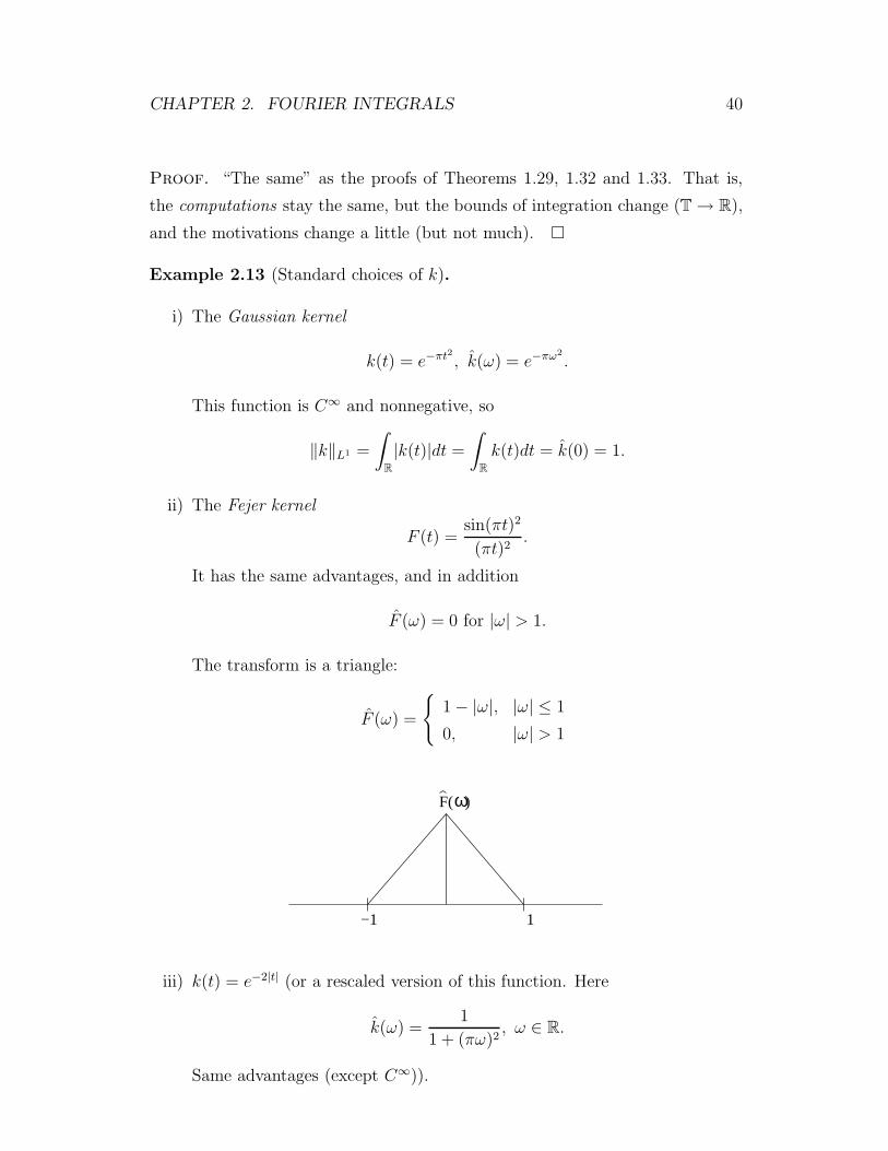
Example 2.13 (Standard choices of k).
i) The Gaussian kernel
k(t) = e−πt2
, k(ω) = e−πω2
.
This function is C∞ and nonnegative, so
‖k‖L1 =
∫
R
|k(t)|dt =
∫
R
k(t)dt = k(0) = 1.
ii) The Fejer kernel
F (t) =sin(πt)2
(πt)2.
It has the same advantages, and in addition
F (ω) = 0 for |ω| > 1.
The transform is a triangle:
F (ω) =
1 − |ω|, |ω| ≤ 1
0, |ω| > 1
−1 1
F( )ω
iii) k(t) = e−2|t| (or a rescaled version of this function. Here
k(ω) =1
1 + (πω)2, ω ∈ R.
Same advantages (except C∞)).

CHAPTER 2. FOURIER INTEGRALS 41
Comment 2.14. According to Theorem 2.7 (e), kλ(ω) → k(0) = 1 as λ →∞, for all ω ∈ R. All the kernels above are “low pass filters” (non causal).
It is possible to use “one-sided” (“causal”) filters instead (i.e., k(t) = 0 for
t < 0). Substituting these into Theorem 2.12 we get “approximate identities”,
which “converge to a δ-distribution”. Details later.
Theorem 2.15. If both f ∈ L1(R) and f ∈ L1(R), then the inversion formula
f(t) =
∫ ∞
−∞e2πiωtf(ω)dω (2.1)
is valid for almost all t ∈ R. By redefining f on a set of measure zero we can
make it hold for all t ∈ R (the right hand side of (2.1) is continuous).
Proof. We approximate∫
Re2πiωtf(ω)dω by
∫Re2πiωte−ε
2πω2f(ω)dω (where ε > 0 is small)
=∫
Re2πiωt−ε
2πω2 ∫Re−2πiωsf(s)dsdω (Fubini)
=∫s∈R
f(s)
∫
ω∈R
e−2πiω(s−t) e−ε2πω2
︸ ︷︷ ︸k(εω2)
dωds
︸ ︷︷ ︸(⋆)
(Ex. 2.13 last page)
(⋆) The Fourier transform of k(εω2) at the point s− t. By Theorem 2.7 (e) this
is equal to
=1
εk(s− t
ε) =
1
εk(t− s
ε)
(since k(ω) = e−πω2
is even).
The whole thing is
∫
s∈R
f(s)1
εk
(t− s
ε
)ds = (f ∗ k 1
ε)(t) → f ∈ L1(R)
as ε→ 0+ according to Theorem 2.12. Thus, for almost all t ∈ R,
f(t) = limε→0
∫
R
e2πiωte−ε2πω2
f(ω)dω.
On the other hand, by the Lebesgue dominated convergence theorem, since
|e2πiωte−ε2πω2
f(ω)| ≤ |f(ω)| ∈ L1(R),
limε→0
∫
R
e2πiωte−ε2πω2
f(ω)dω =
∫
R
e2πiωtf(ω)dω.

CHAPTER 2. FOURIER INTEGRALS 42
Thus, (2.1) holds a.e. The proof of the fact that
∫
R
e2πiωtf(ω)dω ∈ C0(R)
is the same as the proof of Theorem 2.3 (replace t by −t).
The same proof also gives us the following “approximate inversion formula”:
Theorem 2.16. Suppose that k ∈ L1(R), k ∈ L1(R), and that
k(0) =
∫
R
k(t)dt = 1.
If f belongs to one of the function spaces
a) f ∈ Lp(R), 1 ≤ p <∞
b) f ∈ C0(R)
c) f ∈ BUC(R)
then ∫
R
e2πiωtk(εω)f(ω)dω → f(t)
in the norm of the given space (i.e., in Lp-norm, or in the sup-norm), and also
a.e. if∫∞0
(sups≥|t||k(s)|)dt <∞.
Proof. Almost the same as the proof given above. If k is not even, then we
end up with a convolution with the function kε(t) = 1εk(−t/ε) instead, but we
can still apply Theorem 2.12 with k(t) replaced by k(−t).
Corollary 2.17. The inversion in Theorem 2.15 can be interpreted as follows:
If f ∈ L1(R) and f ∈ L1(R), then,
ˆf(t) = f(−t) a.e.
Hereˆf(t) = the Fourier transform of f evaluated at the point t.
Proof. By Theorem 2.15,
f(t) =
∫
R
e−2πi(−t)ω f(ω)dω
︸ ︷︷ ︸Fourier transform of f at the point (−t)
a.e.

CHAPTER 2. FOURIER INTEGRALS 43
Corollary 2.18.ˆˆf(t) = f(t) (If we repeat the Fourier transform 4 times, then
we get back the original function). (True at least if f ∈ L1(R) and f ∈ L1(R). )
As a prelude (=preludium) to the L2-theory we still prove some additional results:
Lemma 2.19. Let f ∈ L1(R) and g ∈ L1(R). Then
∫
R
f(t)g(t)dt =
∫
R
f(s)g(s)ds
Proof.
∫
R
f(t)g(t)dt =
∫
t∈R
f(t)
∫
s∈R
e−2πitsg(s)dsdt (Fubini)
=
∫
s∈R
(∫
t∈R
f(t)e−2πistdt
)g(s)ds
=
∫
s∈R
f(s)g(s)ds.
Theorem 2.20. Let f ∈ L1(R), h ∈ L1(R) and h ∈ L1(R). Then
∫
R
f(t)h(t)dt =
∫
R
f(ω)h(ω)dω. (2.2)
Specifically, if f = h, then (f ∈ L2(R) and)
‖f‖L2(R) = ‖f‖L2(R). (2.3)
Proof. Since h(t) =∫ω∈R
e2πiωth(ω)dω we have
∫
R
f(t)h(t)dt =
∫
t∈R
f(t)
∫
ω∈R
e−2πiωth(ω)dωdt (Fubini)
=
∫
s∈R
(∫
t∈R
f(t)e−2πistdt
)h(ω)dω
=
∫
R
f(ω)h(ω)dω.
2.2 Rapidly Decaying Test Functions
(“Snabbt avtagande testfunktioner”).
Definition 2.21. S = the set of functions f with the following properties
i) f ∈ C∞(R) (infinitely many times differentiable)

CHAPTER 2. FOURIER INTEGRALS 44
ii) tkf (n)(t) → 0 as t→ ±∞ and this is true for all
k, n ∈ Z+ = 0, 1, 2, 3, . . ..
Thus: Every derivative of f → 0 at infinity faster than any negative power of t.
Note: There is no natural norm in this space (it is not a “Banach” space).
However, it is possible to find a complete, shift-invariant metric on this space (it
is a Frechet space).
Example 2.22. f(t) = P (t)e−πt2 ∈ S for every polynomial P (t). For example,
the Hermite functions are of this type (see course in special functions).
Comment 2.23. Gripenberg denotes S by C∞↓ (R). The functions in S are called
rapidly decaying test functions.
The main result of this section is
Theorem 2.24. f ∈ S ⇐⇒ f ∈ S
That is, both the Fourier transform and the inverse Fourier transform maps this
class of functions onto itself. Before proving this we prove the following
Lemma 2.25. We can replace condition (ii) in the definition of the class S by
one of the conditions
iii)∫
R|tkf (n)(t)|dt <∞, k, n ∈ Z+ or
iv) |(ddt
)ntkf(t)| → 0 as t→ ±∞, k, n ∈ Z+
without changing the class of functions S.
Proof. If ii) holds, then for all k, n ∈ Z+,
supt∈R
|(1 + t2)tkf (n)(t)| <∞
(replace k by k + 2 in ii). Thus, for some constant M,
|tkf (n)(t)| ≤ M
1 + t2=⇒
∫
R
|tkf (n)(t)|dt <∞.
Conversely, if iii) holds, then we can define g(t) = tk+1f (n)(t) and get
g′(t) = (k + 1)tkf (n)(t)︸ ︷︷ ︸∈L1
+ tk+1f (n+1)(t)︸ ︷︷ ︸∈L1
,
CHAPTER 2. FOURIER INTEGRALS 45
so g′ ∈ L1(R), i.e., ∫ ∞
−∞|g′(t)|dt <∞.
This implies
|g(t)| ≤ |g(0) +
∫ t
0
g′(s)ds|
≤ |g(0)| +∫ t
0
|g′(s)|ds
≤ |g(0)| +∫ ∞
−∞|g′(s)|ds = |g(0)| + ‖g′‖L1 ,
so g is bounded. Thus,
tkf (n)(t) =1
tg(t) → 0 as t→ ±∞.
The proof that ii) ⇐⇒ iv) is left as a homework.
Proof of Theorem 2.24. By Theorem 2.7, the Fourier transform of
(−2πit)kf (n)(t) is
(d
dω
)k(2πiω)nf(ω).
Therefore, if f ∈ S, then condition iii) on the last page holds, and by Theorem
2.3, f satisfies the condition iv) on the last page. Thus f ∈ S. The same ar-
gument with e−2πiωt replaced by e+2πiωt shows that if f ∈ S, then the Fourier
inverse transform of f (which is f) belongs to S.
Note: Theorem 2.24 is the basis for the theory of Fourier transforms of distribu-
tions. More on this later.
2.3 L2-Theory for Fourier Integrals
As we saw earlier in Lemma 1.10, L2(T) ⊂ L1(T). However, it is not true that
L2(R) ⊂ L1(R). Counter example:
f(t) =1√
1 + t2
∈ L2(R)
6∈ L1(R)
∈ C∞(R)
(too large at ∞).
So how on earth should we define f(ω) for f ∈ L2(R), if the integral∫
R
e−2πintf(t)dt
CHAPTER 2. FOURIER INTEGRALS 46
does not converge?
Recall: Lebesgue integral converges ⇐⇒ converges absolutely ⇐⇒∫|e−2πintf(t)|dt <∞ ⇐⇒ f ∈ L1(R).
We are saved by Theorem 2.20. Notice, in particular, condition (2.3) in that
theorem!
Definition 2.26 (L2-Fourier transform).
i) Approximate f ∈ L2(R) by a sequence fn ∈ S which converges to f in
L2(R). We do this e.g. by “smoothing” and “cutting” (“utjamning” och
“klippning”): Let k(t) = e−πt2, define
kn(t) = nk(nt), and
fn(t) = k
(t
n
)
︸ ︷︷ ︸⋆
(kn ∗ f)(t)︸ ︷︷ ︸⋆⋆
︸ ︷︷ ︸the product belongs to S
(⋆) this tends to zero faster than any polynomial as t→ ∞.
(⋆⋆) “smoothing” by an approximate identity, belongs toC∞ and is bounded.
By Theorem 2.12 kn ∗ f → f in L2 as n → ∞. The functions k(tn
)tend
to k(0) = 1 at every point t as n → ∞, and they are uniformly bounded
by 1. By using the appropriate version of the Lesbesgue convergence we
let fn → f in L2(R) as n→ ∞.
ii) Since fn converges in L2, also fn must converge to something in L2. More
about this in “Analysis II”. This follows from Theorem 2.20. (fn → f ⇒fn Cauchy sequence ⇒ fn Cauchy seqence ⇒ fn converges.)
iii) Call the limit to which fn converges “The Fourier transform of f”, and
denote it f .
Definition 2.27 (Inverse Fourier transform). We do exactly as above, but re-
place e−2πiωt by e+2πiωt.
Final conclusion:

CHAPTER 2. FOURIER INTEGRALS 47
Theorem 2.28. The “extended” Fourier transform which we have defined above
has the following properties: It maps L2(R) one-to-one onto L2(R), and if f is the
Fourier transform of f , then f is the inverse Fourier transform of f . Moreover,
all norms, distances and inner products are preserved.
Explanation:
i) “Normes preserved” means∫
R
|f(t)|2dt =
∫
R
|f(ω)|2dω,
or equivalently, ‖f‖L2(R) = ‖f‖L2(R).
ii) “Distances preserved” means
‖f − g‖L2(R) = ‖f − g‖L2(R)
(apply i) with f replaced by f − g)
iii) “Inner product preserved” means∫
R
f(t)g(t)dt =
∫
R
f(ω)g(ω)dω,
which is often written as
〈f, g〉L2(R) = 〈f , g〉L2(R).
This was theory. How to do in practice?
One answer: We saw earlier that if [a, b] is a finite interval, and if f ∈ L2[a, b] ⇒f ∈ L1[a, b], so for each T > 0, the integral
fT (ω) =
∫ T
−Te−2πiωtf(t)dt
is defined for all ω ∈ R. We can try to let T → ∞, and see what happens. (This
resembles the theory for the inversion formula for the periodical L2-theory.)
Theorem 2.29. Suppose that f ∈ L2(R). Then
limT→∞
∫ T
−Te−2πiωtf(t)dt = f(ω)
in the L2-sense as T → ∞, and likewise
limT→∞
∫ T
−Te2πiωtf(ω)dω = f(t)
in the L2-sense.

CHAPTER 2. FOURIER INTEGRALS 48
Proof. Much too hard to be presented here. Another possibility: Use the Fejer
kernel or the Gaussian kernel, or any other kernel, and define
f(ω) = limn→∞∫
Re−2πiωtk
(tn
)f(t)dt,
f(t) = limn→∞∫
Re+2πiωtk
(ωn
)f(ω)dω.
We typically have the same type of convergence as we had in the Fourier inversion
formula in the periodic case. (This is a well-developed part of mathematics, with
lots of results available.) See Gripenberg’s compendium for some additional
results.
2.4 An Inversion Theorem
From time to time we need a better (= more useful) inversion theorem for the
Fourier transform, so let us prove one here:
Theorem 2.30. Suppose that f ∈ L1(R) + L2(R) (i.e., f = f1 + f2, where
f1 ∈ L1(R) and f2 ∈ L2(R)). Let t0 ∈ R, and suppose that
∫ t0+1
t0−1
∣∣∣f(t) − f(t0)
t− t0
∣∣∣dt <∞. (2.4)
Then
f(t0) = limS→∞T→∞
∫ T
−Se2πiωt0 f(ω)dω, (2.5)
where f(ω) = f1(ω) + f2(ω).
Comment: Condition (2.4) is true if, for example, f is differentiable at the point
t0.
Proof. Step 1. First replace f(t) by g(t) = f(t+ t0). Then
g(ω) = e2πiωt0 f(ω),
and (2.5) becomes
g(0) = limS→∞T→∞
∫ T
−Sg(ω)dω,
and (2.4) becomes ∫ 1
−1
∣∣∣g(t− t0) − g(0)
t− t0
∣∣∣dt <∞.
Thus, it suffices to prove the case where t0 = 0 .
CHAPTER 2. FOURIER INTEGRALS 49
Step 2: We know that the theorem is true if g(t) = e−πt2
(See Example 2.5 and
Theorem 2.15). Replace g(t) by
h(t) = g(t) − g(0)e−πt2
.
Then h satisfies all the assumptions which g does, and in addition, h(0) = 0.
Thus it suffices to prove the case where both (⋆) t0 = 0 and f(0) = 0 .
For simplicity we write f instead of h but assume (⋆). Then (2.4) and (2.5)
simplify:
∫ 1
−1
∣∣∣f(t)
t
∣∣∣dt < ∞, (2.6)
limS→∞T→∞
∫ T
−Sf(ω)dω = 0. (2.7)
Step 3: If f ∈ L1(R), then we argue as follows. Define
g(t) =f(t)
−2πit.
Then g ∈ L1(R). By Fubini’s theorem,
∫ T
−Sf(ω)dω =
∫ T
−S
∫ ∞
−∞e−2πiωtf(t)dtdω
=
∫ ∞
−∞
∫ T
−Se−2πiωtdωf(t)dt
=
∫ ∞
−∞
[1
−2πite−2πiωt
]T
−Sf(t)dt
=
∫ ∞
−∞
[e−2πiT t − e−2πi(−S)t
] f(t)
−2πitdt
= g(T ) − g(−S),
and this tends to zero as T → ∞ and S → ∞ (see Theorem 2.3). This proves
(2.7).
Step 4: If instead f ∈ L2(R), then we use Parseval’s identity
∫ ∞
−∞f(t)h(t)dt =
∫ ∞
−∞f(ω)h(ω)dω
in a clever way: Choose
h(ω) =
1, −S ≤ t ≤ T,
0, otherwise.
CHAPTER 2. FOURIER INTEGRALS 50
Then the inverse Fourier transform h(t) of h is
h(t) =
∫ T
−Se2πiωtdω
=
[1
2πite2πiωt
]T
−S=
1
2πit
[e2πiT t − e2πi(−S)t
]
so Parseval’s identity gives
∫ T
−Sf(ω)dω =
∫ ∞
−∞f(t)
1
−2πit
[e−2πiT t − e−2πi(−S)t
]dt
= (with g(t) as in Step 3)
=
∫ ∞
−∞
[e−2πiT t − e−2πi(S)t
]g(t)dt
= g(T ) − g(−S) → 0 as
T → ∞,
S → ∞.
Step 5: If f = f1 + f2, where f1 ∈ L1(R) and f2 ∈ L2(R), then we apply Step 3
to f1 and Step 4 to f2, and get in both cases (2.7) with f replaced by f1 and f2.
Note: This means that in “most cases” where f is continuous at t0 we have
f(t0) = limS→∞T→∞
∫ T
−Se2πiωt0 f(ω)dω.
(continuous functions which do not satisfy (2.4) do exist, but they are difficult
to find.) In some cases we can even use the inversion formula at a point where
f is discontinuous.
Theorem 2.31. Suppose that f ∈ L1(R) + L2(R). Let t0 ∈ R, and suppose that
the two limits
f(t0+) = limt↓t0
f(t)
f(t0−) = limt↑t0
f(t)
exist, and that
∫ t0+1
t0
∣∣∣f(t) − f(t0+)
t− t0
∣∣∣dt < ∞,
∫ t0
t0−1
∣∣∣f(t) − f(t0−)
t− t0
∣∣∣dt < ∞.

CHAPTER 2. FOURIER INTEGRALS 51
Then
limT→∞
∫ T
−Te2πiωt0 f(ω)dω =
1
2[f(t0+) + f(t0−)].
Note: Here we integrate∫ T−T , not
∫ T−S, and the result is the average of the right
and left hand limits.
Proof. As in the proof of Theorem 2.30 we may assume that
Step 1: t0 = 0 , (see Step 1 of that proof)
Step 2: f(t0+) + f(t0−) = 0 , (see Step 2 of that proof).
Step 3: The claim is true in the special case where
g(t) =
e−t, t > 0,
−et, t < 0,
because g(0+) = 1, g(0−) = −1, g(0+) + g(0−) = 0, and∫ T
−Tg(ω)dω = 0 for all T,
since f is odd =⇒ g is odd.
Step 4: Define h(t) = f(t)−f(0+) · g(t), where g is the function in Step 3. Then
h(0+) = f(0+) − f(0+) = 0 and
h(0−) = f(0−) − f(0+)(−1) = 0, so
h is continuous. Now apply Theorem 2.30 to h. It gives
0 = h(0) = limT→∞
∫ T
−Th(ω)dω.
Since also
0 = f(0+)[g(0+) + g(0−)] = limT→∞
∫ T
−Tg(ω)dω,
we therefore get
0 = f(0+) + f(0−) = limT→∞
∫ T
−T[h(ω) + g(ω)]dω = lim
T→∞
∫ T
−Tf(ω)dω.
Comment 2.32. Theorems 2.30 and 2.31 also remain true if we replace
limT→∞
∫ T
−Te2πiωtf(ω)dω
by
limε→0
∫ ∞
−∞e2πiωte−π(εω)2 f(ω)dω (2.8)
(and other similar “summability” formulas). Compare this to Theorem 2.16. In
the case of Theorem 2.31 it is important that the “cutoff kernel” (= e−π(εω)2 in
(2.8)) is even.

CHAPTER 2. FOURIER INTEGRALS 52
2.5 Applications
2.5.1 The Poisson Summation Formula
Suppose that f ∈ L1(R) ∩ C(R), that∑∞
n=−∞|f(n)| < ∞ (i.e., f ∈ ℓ1(Z)), and
that∑∞
n=−∞ f(t+n) converges uniformly for all t in some interval (−δ, δ). Then
∞∑
n=−∞f(n) =
∞∑
n=−∞f(n) (2.9)
Note: The uniform convergence of∑f(t + n) can be difficult to check. One
possible way out is: If we define
εn = sup−δ<t<δ
|f(t+ n)|,
and if∑∞
n=−∞ εn < ∞, then∑∞
n=−∞ f(t + n) converges (even absolutely), and
the convergence is uniform in (−δ, δ). The proof is roughly the same as what we
did on page 29.
Proof of (2.9). We first construct a periodic function g ∈ L1(T) with the
Fourier coefficients f(n):
f(n) =
∫ ∞
−∞e−2πintf(t)dt
=∞∑
k=−∞
∫ k+1
k
e−2πintf(t)dt
t=k+s=
∞∑
k=−∞
∫ 1
0
e−2πinsf(s+ k)ds
Thm 0.14=
∫ 1
0
e−2πins
( ∞∑
k=−∞f(s+ k)
)ds
= g(n), where g(t) =
∞∑
n=−∞f(t+ n).
(For this part of the proof it is enough to have f ∈ L1(R). The other conditions
are needed later.)
So we have g(n) = f(n). By the inversion formula for the periodic Fourier
transform:
g(0) =
∞∑
n=−∞e2πin0g(n) =
∞∑
n=−∞g(n) =
∞∑
n=−∞f(n),

CHAPTER 2. FOURIER INTEGRALS 53
provided (=forutsatt) that we are allowed to use the Fourier inversion formula.
This is allowed if g ∈ C[−δ, δ] and g ∈ ℓ1(Z) (Theorem 1.37). This was part of
our assumption.
In addition we need to know that the formula
g(t) =
∞∑
n=−∞f(t+ n)
holds at the point t = 0 (almost everywhere is no good, we need it in exactly
this point). This is OK if∑∞
n=−∞ f(t + n) converges uniformly in [−δ, δ] (this
also implies that the limit function g is continuous).
Note: By working harder in the proof, Gripenberg is able to weaken some of the
assumptions. There are also some counter-examples on how things can go wrong
if you try to weaken the assumptions in the wrong way.
2.5.2 Is L1(R) = C0(R) ?
That is, is every function g ∈ C0(R) the Fourier transform of a function f ∈L1(R)?
The answer is no, as the following counter-example shows. Take
g(ω) =
ωln 2
, |ω| ≤ 1,1
ln(1+ω), ω > 1,
− 1ln(1−ω)
, ω < −1.
Suppose that this would be the Fourier transform of a function f ∈ L1(R). As
in the proof on the previous page, we define
h(t) =∞∑
n=−∞f(t+ n).
Then (as we saw there), h ∈ L1(T), and h(n) = f(n) for n = 0,±1,±2, . . ..
However, since∑∞
n=11nh(n) = ∞, this is not the Fourier sequence of any h ∈
L1(T) (by Theorem 1.38). Thus:
Not every h ∈ C0(R) is the Fourier transform of some f ∈ L1(R).
But:
f ∈ L1(R) ⇒ f ∈ C0(R) ( Page 36)
f ∈ L2(R) ⇔ f ∈ L2(R) ( Page 47)
f ∈ S ⇔ f ∈ S ( Page 44)

CHAPTER 2. FOURIER INTEGRALS 54
2.5.3 The Euler-MacLauren Summation Formula
Let f ∈ C∞(R+) (where R+ = [0,∞)), and suppose that
f (n) ∈ L1(R+)
for all n ∈ Z+ = 0, 1, 2, 3 . . .. We define f(t) for t < 0 so that f(t) is even.
Warning: f is continuous at the origin, but f ′ may be discontinuous! For exam-
ple, f(t) = e−|2t|
f(t)=e −2|t|
We want to use Poisson summation formula. Is this allowed?
By Theorem 2.7, f (n) = (2πiω)nf(ω), and f (n) is bounded, so
supω∈R
|(2πiω)n||f(ω)| <∞ for all n ⇒∞∑
n=−∞|f(n)| <∞.
By the note on page 52, also∑∞
n=−∞ f(t+n) converges uniformly in (−1, 1). By
the Poisson summation formula:
∞∑
n=0
f(n) =1
2f(0) +
1
2
∞∑
n=−∞f(n)
=1
2f(0) +
1
2
∞∑
n=−∞f(n)
=1
2f(0) +
1
2f(0) +
1
2
∞∑
n=1
[f(n) + f(−n)
]
=1
2f(0) +
1
2f(0) +
∞∑
n=1
∫ ∞
−∞
1
2
(e2πint + e−2πint
)︸ ︷︷ ︸
cos(2πnt)
f(t)dt
=1
2f(0) +
∫ ∞
0
f(t)dt+
∞∑
n=1
∫ ∞
0
cos(2πnt)f(t)dt
Here we integrate by parts several times, always integrating the cosine-function
and differentiating f . All the substitution terms containing odd derivatives of
CHAPTER 2. FOURIER INTEGRALS 55
f vanish since sin(2πnt) = 0 for t = 0. See Gripenberg for details. The result
looks something like
∞∑
n=0
f(n) =
∫ ∞
0
f(t)dt+1
2f(0) − 1
12f ′(0) +
1
720f ′′′(0) − 1
30240f (5)(0) + . . .
2.5.4 Schwartz inequality
The Schwartz inequality will be used below. It says that
|〈f, g〉| ≤ ‖f‖L2‖g‖L2
(true for all possible L2-spaces, both L2(R) and L2(T) etc.)
2.5.5 Heisenberg’s Uncertainty Principle
For all f ∈ L2(R), we have
(∫ ∞
−∞t2|f(t)|2dt
)(∫ ∞
−∞ω2|f(ω)|2dω
)≥ 1
16π2
∥∥f∥∥4
L2(R)
Interpretation: The more concentrated f is in the neighborhood of zero, the
more spread out must f be, and conversely. (Here we must think that ‖f‖L2(R)
is fixed, e.g. ‖f‖L2(R) = 1.)
In quantum mechanics: The product of “time uncertainty” and “space uncer-
tainty” cannot be less than a given fixed number.

CHAPTER 2. FOURIER INTEGRALS 56
Proof. We begin with the case where f ∈ S. Then
16π
∫
R
|tf(t)|dt∫
R
|ωf(ω)|dω = 4
∫
R
|tf(t)|dt∫
R
|f ′(t)|dt
(f ′(ω) = 2πiωf(ω) and Parseval’s iden. holds). Now use Scwartz ineq.
≥ 4
(∫
R
|tf(t)||f ′(t)|dt)
= 4
(∫
R
|tf(t)||f ′(t)|dt)
≥ 4
(∫
R
Re[tf(t)f ′(t)]dt
)
= 4
(∫
R
t
[1
2
(f(t)f ′(t) + f(t)f ′(t)
)]dt
)2
=
∫
R
td
dt(f(t)f(t))︸ ︷︷ ︸
=|f(t)|
dt (integrate by parts)
=([t|f(t)|]∞−∞︸ ︷︷ ︸
=0
−∫ ∞
−∞|f(t)|dt
)
=
(∫ ∞
−∞|f(t)|dt
)
This proves the case where f ∈ S. If f ∈ L(R), but f ∈ S, then we choose a
sequence of functions fn ∈ S so that
∫ ∞
−∞|fn(t)|dt →
∫ ∞
−∞|f(t)|dt and
∫ ∞
−∞|tfn(t)|dt →
∫ ∞
−∞|tf(t)|dt and
∫ ∞
−∞|ωfn(ω)|dω →
∫ ∞
−∞|ωf(ω)|dω
(This can be done, not quite obvious). Since the inequality holds for each fn, it
must also hold for f .
2.5.6 Weierstrass’ Non-Differentiable Function
Define σ(t) =∑∞
k=0 ak cos(2πbkt), t ∈ R where 0 < a < 1 and ab≥ 1.
Lemma 2.33. This sum defines a continuous function σ which is not differ-
entiable at any point.

CHAPTER 2. FOURIER INTEGRALS 57
Proof. Convergence easy: At each t,
∞∑
k=0
|ak cos(2πbkt)| ≤∞∑
k=0
ak =1
1 − a<∞,
and absolute convergence ⇒ convergence. The convergence is even uniform: The
error is
∣∣∞∑
k=K
ak cos(2πbkt)∣∣ ≤
∞∑
k=K
|ak cos(2πbkt)| ≤∞∑
k=K
ak =aK
1 − a→ 0 as K → ∞
so by choosing K large enough we can make the error smaller than ε, and the
same K works for all t.
By “Analysis II”: If a sequence of continuous functions converges uniformly, then
the limit function is continuous. Thus, σ is continuous.
Why is it not differentiable? At least does the formal derivative not converge:
Formally we should have
σ′(t) =
∞∑
k=0
ak · 2πbk(−1) sin(2πbkt),
and the terms in this serie do not seem to go to zero (since (ab)k ≥ 1). (If a sum
converges, then the terms must tend to zero.)
To prove that σ is not differentiable we cut the sum appropriatly: Choose some
function ϕ ∈ L1(R) with the following properties:
i) ϕ(1) = 1
ii) ϕ(ω) = 0 for ω ≤ 1b
and ω > b
iii)∫∞−∞|tϕ(t)|dt <∞.
0 1/b 1 b
ϕ(ω)
We can get such a function from the Fejer kernel: Take the square of the Fejer
kernel (⇒ its Fourier transform is the convolution of f with itself), squeeze it
(Theorem 2.7(e)), and shift it (Theorem 2.7(b)) so that it vanishes outside of
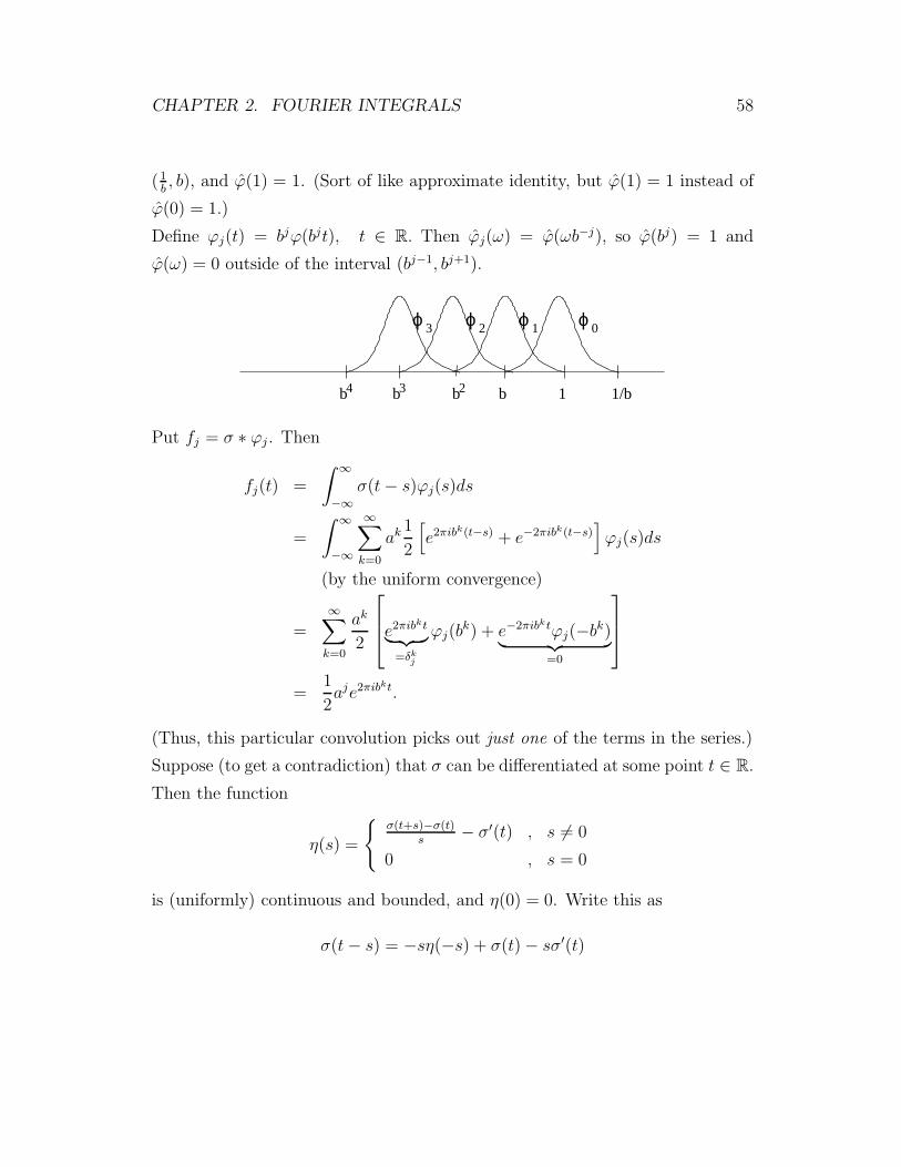
CHAPTER 2. FOURIER INTEGRALS 58
(1b, b), and ϕ(1) = 1. (Sort of like approximate identity, but ϕ(1) = 1 instead of
ϕ(0) = 1.)
Define ϕj(t) = bjϕ(bjt), t ∈ R. Then ϕj(ω) = ϕ(ωb−j), so ϕ(bj) = 1 and
ϕ(ω) = 0 outside of the interval (bj−1, bj+1).
ϕ 0ϕ 1ϕ 2ϕ 3
b4 b3 b2 b 1 1/b
Put fj = σ ∗ ϕj . Then
fj(t) =
∫ ∞
−∞σ(t− s)ϕj(s)ds
=
∫ ∞
−∞
∞∑
k=0
ak1
2
[e2πib
k(t−s) + e−2πibk(t−s)]ϕj(s)ds
(by the uniform convergence)
=∞∑
k=0
ak
2
e2πibkt︸ ︷︷ ︸
=δkj
ϕj(bk) + e−2πibktϕj(−bk)︸ ︷︷ ︸
=0
=1
2aje2πib
kt.
(Thus, this particular convolution picks out just one of the terms in the series.)
Suppose (to get a contradiction) that σ can be differentiated at some point t ∈ R.
Then the function
η(s) =
σ(t+s)−σ(t)
s− σ′(t) , s 6= 0
0 , s = 0
is (uniformly) continuous and bounded, and η(0) = 0. Write this as
σ(t− s) = −sη(−s) + σ(t) − sσ′(t)

CHAPTER 2. FOURIER INTEGRALS 59
i.e.,
fj(t) =
∫
R
σ(t− s)ϕj(s)ds
=
∫
R
−sη(−s)ϕj(s)ds+ σ(t)
∫
R
ϕj(s)ds
︸ ︷︷ ︸=ϕj(0)=0
−σ′(t)
∫
R
sϕj(s)ds
︸ ︷︷ ︸ϕ′
j(0)
−2πi=0
= −∫
R
sη(−s)bjϕ(bjs)ds
bjs=t= −bj
∫
R
η(−sbj
)︸ ︷︷ ︸
→0 pointwise
sϕ(s)ds︸ ︷︷ ︸∈L1
→ 0 by the Lesbesgue dominated convergence theorem as j → ∞.
Thus,
b−jfj(t) → 0 as j → ∞ ⇔ 1
2
(ab
)je2πib
jt → 0 as j → ∞.
As |e2πibjt| = 1, this is ⇔(ab
)j → 0 as j → ∞. Impossible, since ab≥ 1. Our
assumption that σ is differentiable at the point t must be wrong ⇒ σ(t) is not
differentiable in any point!
2.5.7 Differential Equations
Solve the differential equation
u′′(t) + λu(t) = f(t), t ∈ R (2.10)
where we require that f ∈ L2(R), u ∈ L2(R), u ∈ C1(R), u′ ∈ L2(R) and that u′
is of the form
u′(t) = u′(0) +
∫ t
0
v(s)ds,
where v ∈ L2(R) (that is, u′ is “absolutely continuous” and its “generalized
derivative” belongs to L2).
The solution of this problem is based on the following lemmas:
Lemma 2.34. Let k = 1, 2, 3, . . .. Then the following conditions are equivalent:
i) u ∈ L2(R)∩Ck−1(R), u(k−1) is “absolutely continuous” and the “generalized
derivative of u(k−1)” belongs to L2(R).
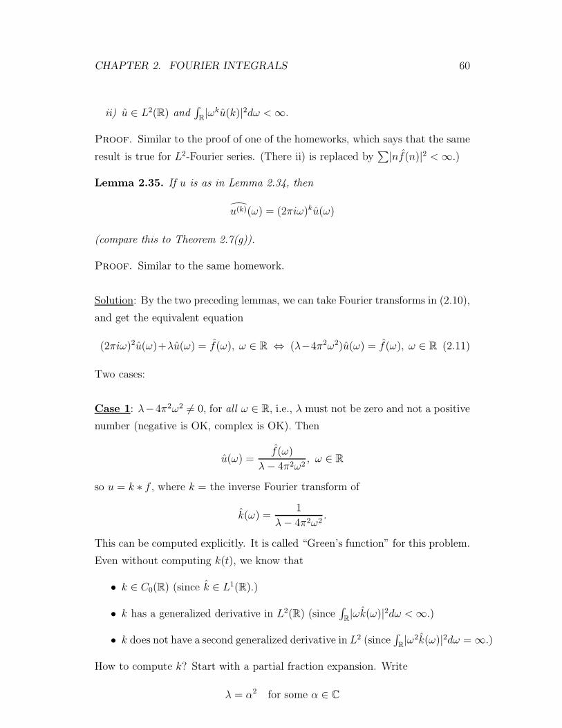
CHAPTER 2. FOURIER INTEGRALS 60
ii) u ∈ L2(R) and∫
R|ωku(k)|2dω <∞.
Proof. Similar to the proof of one of the homeworks, which says that the same
result is true for L2-Fourier series. (There ii) is replaced by∑
|nf(n)|2 <∞.)
Lemma 2.35. If u is as in Lemma 2.34, then
u(k)(ω) = (2πiω)ku(ω)
(compare this to Theorem 2.7(g)).
Proof. Similar to the same homework.
Solution: By the two preceding lemmas, we can take Fourier transforms in (2.10),
and get the equivalent equation
(2πiω)2u(ω)+λu(ω) = f(ω), ω ∈ R ⇔ (λ−4π2ω2)u(ω) = f(ω), ω ∈ R (2.11)
Two cases:
Case 1: λ−4π2ω2 6= 0, for all ω ∈ R, i.e., λ must not be zero and not a positive
number (negative is OK, complex is OK). Then
u(ω) =f(ω)
λ− 4π2ω2, ω ∈ R
so u = k ∗ f , where k = the inverse Fourier transform of
k(ω) =1
λ− 4π2ω2.
This can be computed explicitly. It is called “Green’s function” for this problem.
Even without computing k(t), we know that
• k ∈ C0(R) (since k ∈ L1(R).)
• k has a generalized derivative in L2(R) (since∫
R|ωk(ω)|2dω <∞.)
• k does not have a second generalized derivative in L2 (since∫
R|ω2k(ω)|2dω = ∞.)
How to compute k? Start with a partial fraction expansion. Write
λ = α2 for some α ∈ C

CHAPTER 2. FOURIER INTEGRALS 61
(α = pure imaginary if λ < 0). Then
1
λ− 4π2ω2=
1
α2 − 4π2ω2=
1
α− 2πω· 1
α+ 2πω
=A
α− 2πω+
B
α + 2πω
=Aα + 2πωA+Bα− 2πωB
(α− 2πω)(α+ 2πω)
⇒ (A+B)α = 1
(A− B)2πω = 0
⇒ A = B =
1
2α
Now we must still invert 1α+2πω
and 1α−2πω
. This we do as follows:
Auxiliary result 1: Compute the transform of
f(t) =
e−zt , t ≥ 0,
0 , t < 0,
where Re(z) > 0 (⇒ f ∈ L2(R) ∩L1(R), but f /∈ C(R) because of the jump at
the origin). Simply compute:
f(ω) =
∫ ∞
0
e−2πiωte−ztdt
=
[e−(z+2πiω)t
−(z + 2πiω)
]∞
0
=1
2πiω + z.
Auxiliary result 2: Compute the transform of
f(t) =
ezt , t ≤ 0,
0 , t > 0,
where Re(z) > 0 (⇒ f ∈ L2(R) ∩ L1(R), but f /∈ C(R))
⇒ f(ω) =
∫ 0
−∞e2πiωteztdt
=
[e(z−2πiω)t
(z − 2πiω)t
]0
−∞=
1
z − 2πiω.
Back to the function k:
k(ω) =1
2α
(1
α− 2πω+
1
α + 2πω
)
=1
2α
(i
iα− 2πiω+
i
iα + 2πiω
).
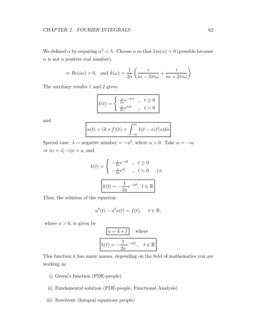
CHAPTER 2. FOURIER INTEGRALS 62
We defined α by requiring α2 = λ. Choose α so that Im(α) < 0 (possible because
α is not a positive real number).
⇒ Re(iα) > 0, and k(ω) =1
2α
(i
iα− 2πiω+
i
iα + 2πiω
)
The auxiliary results 1 and 2 gives:
k(t) =
i
2αe−iαt , t ≥ 0
i2αeiαt , t < 0
and
u(t) = (k ∗ f)(t) =
∫ ∞
−∞k(t− s)f(s)ds
Special case: λ = negative number = −a2, where a > 0. Take α = −ia⇒ iα = i(−i)a = a, and
k(t) =
− 1
2ae−at , t ≥ 0
− 12aeat , t < 0 i.e.
k(t) = − 1
2ae−|at|, t ∈ R
Thus, the solution of the equation
u′′(t) − a2u(t) = f(t), t ∈ R,
where a > 0, is given by
u = k ∗ f where
k(t) = − 1
2ae−a|t|, t ∈ R
This function k has many names, depending on the field of mathematics you are
working in:
i) Green’s function (PDE-people)
ii) Fundamental solution (PDE-people, Functional Analysis)
iii) Resolvent (Integral equations people)

CHAPTER 2. FOURIER INTEGRALS 63
Case 2: λ = a2 = a nonnegative number. Then
f(ω) = (a2 − 4π2ω2)u(ω) = (a− 2πω)(a+ 2πω)u(ω).
As u(ω) ∈ L2(R) we get a necessary condition for the existence of a solution: If
a solution exists then
∫
R
∣∣ f(ω)
(a− 2πω)(a+ 2πω)
∣∣2dω <∞. (2.12)
(Since the denominator vanishes for ω = ± a2π
, this forces f to vanish at ± a2π
,
and to be “small” near these points.)
If the condition (2.12) holds, then we can continue the solution as before.
Sideremark: These results mean that this particular problem has no “eigenval-
ues” and no “eigenfunctions”. Instead it has a “contionuous spectrum” consisting
of the positive real line. (Ignore this comment!)
2.5.8 Heat equation
This equation:
∂∂tu(t, x) = ∂2
∂x2u(t, x) + g(t, x),
t > 0
x ∈ R
u(0, x) = f(x) (initial value)
is solved in the same way. Rather than proving everything we proceed in a formal
mannor (everything can be proved, but it takes a lot of time and energy.)
Transform the equation in the x-direction,
u(t, γ) =
∫
R
e−2πiγxu(t, x)dx.
Assuming that∫
Re−2πiγx ∂
∂tu(t, x) = ∂
∂t
∫Re−2πiγxu(t, x)dx we get
∂∂tu(t, γ) = (2πiγ)2u(t, γ) + g(t, γ)
u(0, γ) = f(γ)
⇔∂∂tu(t, γ) = −4π2γ2u(t, γ) + g(t, γ)
u(0, γ) = f(γ)

CHAPTER 2. FOURIER INTEGRALS 64
We solve this by using the standard “variation of constants lemma”:
u(t, γ) = f(γ)e−4π2γ2t
︸ ︷︷ ︸ +
∫ t
0
e−4π2γ2(t−s)g(s, γ)ds
︸ ︷︷ ︸= u1(t, γ) + u2(t, γ)
We can invert e−4π2γ2t = e−π(2√πtγ)2 = e−π(γ/λ)2 where λ = (2
√πt)−1:
According to Theorem 2.7 and Example 2.5, this is the transform of
k(t, x) =1
2√πte−π( x
2√
πt)2
=1
2√πte−
x2
4t
We know that f(γ)k(γ) = k ∗ f(γ), so
u1(t, x) =∫∞−∞
12√πte−(x−y)2/4tf(y)dy,
(By the same argument:
s and t− s are fixed when we transform.)
u2(t, x) =∫ t0(k ∗ g)(s)ds
=∫ t0
∫∞−∞
1
2√π(t−s)
e−(x−y)2/4(t−s)g(s, y)dyds,
u(t, x) = u1(t, x) + u2(t, x)
The function
k(t, x) =1
2√πte−
x2
4t
is the Green’s function or the fundamental solution of the heat equation on the
real line R = (−∞,∞), or the heat kernel.
Note: To prove that this “solution” is indeed a solution we need to assume that
- all functions are in L2(R) with respect to x, i.e.,∫ ∞
−∞|u(t, x)|2dx <∞,
∫ ∞
−∞|g(t, x)|2dx <∞,
∫ ∞
−∞|f(x)|2dx <∞,
- some (weak) continuity assumptions with respect to t.
2.5.9 Wave equation
∂2
∂t2u(t, x) = ∂2
∂x2u(t, x) + k(t, x),
t > 0,
x ∈ R.
u(0, x) = f(x), x ∈ R
∂∂tu(0, x) = g(x), x ∈ R
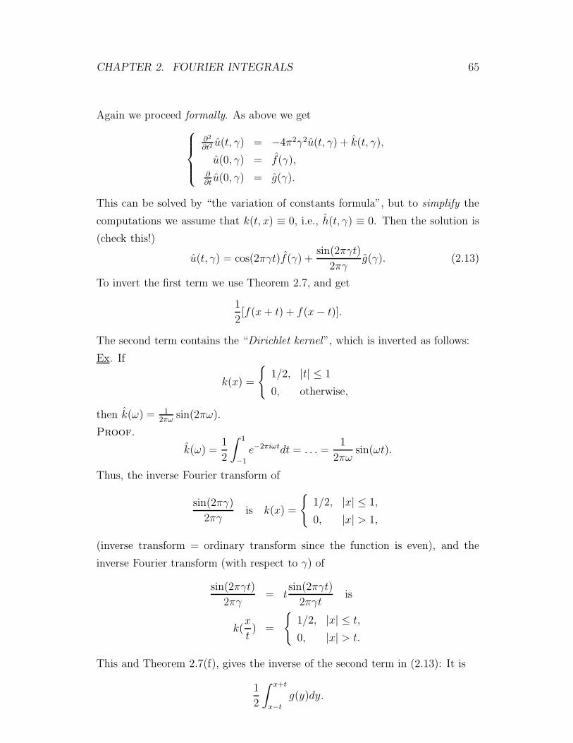
CHAPTER 2. FOURIER INTEGRALS 65
Again we proceed formally. As above we get
∂2
∂t2u(t, γ) = −4π2γ2u(t, γ) + k(t, γ),
u(0, γ) = f(γ),∂∂tu(0, γ) = g(γ).
This can be solved by “the variation of constants formula”, but to simplify the
computations we assume that k(t, x) ≡ 0, i.e., h(t, γ) ≡ 0. Then the solution is
(check this!)
u(t, γ) = cos(2πγt)f(γ) +sin(2πγt)
2πγg(γ). (2.13)
To invert the first term we use Theorem 2.7, and get
1
2[f(x+ t) + f(x− t)].
The second term contains the “Dirichlet kernel”, which is inverted as follows:
Ex. If
k(x) =
1/2, |t| ≤ 1
0, otherwise,
then k(ω) = 12πω
sin(2πω).
Proof.
k(ω) =1
2
∫ 1
−1
e−2πiωtdt = . . . =1
2πωsin(ωt).
Thus, the inverse Fourier transform of
sin(2πγ)
2πγis k(x) =
1/2, |x| ≤ 1,
0, |x| > 1,
(inverse transform = ordinary transform since the function is even), and the
inverse Fourier transform (with respect to γ) of
sin(2πγt)
2πγ= t
sin(2πγt)
2πγtis
k(x
t) =
1/2, |x| ≤ t,
0, |x| > t.
This and Theorem 2.7(f), gives the inverse of the second term in (2.13): It is
1
2
∫ x+t
x−tg(y)dy.

CHAPTER 2. FOURIER INTEGRALS 66
Conclusion: The solution of the wave equation with h(t, x) ≡ 0 seems to be
u(t, x) =1
2[f(x+ t) + f(x− t)] +
1
2
∫ x+t
x−tg(y)dy,
a formula known as d’Alembert’s formula.
Interpretation: This is the sum of two waves: u(t, x) = u+(t, x)+u−(t, x), where
u+(t, x) =1
2f(x+ t) +
1
2G(x+ t)
moves to the left with speed one, and
u−(t, x) =1
2f(x− t) − 1
2G(x− t)
moves to the right with speed one. Here
G(x) =
∫ x
0
g(y)dy, x ∈ R.

Chapter 3
Fourier Transforms of
Distributions
Questions
1) How do we transform a function f /∈ L1(R), f /∈ L2(R), for example
Weierstrass function
σ(t) =
∞∑
k=0
ak cos(2πbkt),
where b 6= integer (if b is an integer, then σ is periodic and we can use
Chapter I)?
2) Can we interpret both the periodic F -transform (on L1(T)) and the Fourier
integral (on L1(R)) as special cases of a “more general” Fourier transform?
3) How do you differentiate a discontinuous function?
The answer: Use “distribution theory”, developed in France by Schwartz in
1950’s.
3.1 What is a Measure?
We start with a simpler question: what is a “δ-function”? Typical definition:
δ(x) = 0, x 6= 0
δ(0) = ∞∫ ε−ε δ(x)dx = 1, (for ε > 0).
67
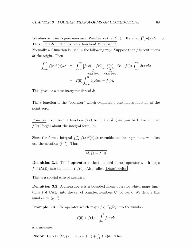
CHAPTER 3. FOURIER TRANSFORMS OF DISTRIBUTIONS 68
We observe: This is pure nonsense. We observe that δ(x) = 0 a.e., so∫ ε−ε δ(x)dx = 0.
Thus: The δ-function is not a function! What is it?
Normally a δ-function is used in the following way: Suppose that f is continuous
at the origin. Then
∫ ∞
−∞f(x)δ(x)dx =
∫ ∞
−∞[f(x) − f(0)]︸ ︷︷ ︸
=0when x=0
δ(x)︸︷︷︸=0
when x 6=0
dx+ f(0)
∫ ∞
−∞δ(x)dx
= f(0)
∫ ∞
−∞δ(x)dx = f(0).
This gives us a new interpretation of δ:
The δ-function is the “operator” which evaluates a continuous function at the
point zero.
Principle: You feed a function f(x) to δ, and δ gives you back the number
f(0) (forget about the integral formula).
Since the formal integral∫∞−∞ f(x)δ(x)dx resembles an inner product, we often
use the notation 〈δ, f〉. Thus
〈δ, f〉 = f(0)
Definition 3.1. The δ-operator is the (bounded linear) operator which maps
f ∈ C0(R) into the number f(0). Also called Dirac’s delta .
This is a special case of measure:
Definition 3.2. A measure µ is a bounded linear operator which maps func-
tions f ∈ C0(R) into the set of complex numbers C (or real). We denote this
number by 〈µ, f〉.
Example 3.3. The operator which maps f ∈ C0(R) into the number
f(0) + f(1) +
∫ 1
0
f(s)ds
is a measure.
Proof. Denote 〈G, f〉 = f(0) + f(1) +∫ 1
0f(s)ds. Then
CHAPTER 3. FOURIER TRANSFORMS OF DISTRIBUTIONS 69
i) G maps C0(R) → C.
ii) G is linear :
〈G, λf + µg〉 = λf(0) + µg(0) + λf(1) + µg(1)
+
∫ 1
0
(λf(s) + µg(s))ds
= λf(0) + λf(1) +
∫ 1
0
λf(s)ds
+µg(0) + µg(1) +
∫ 1
0
µg(s)ds
= λ〈G, f〉 + µ〈G, g〉.
iii) G is continuous : If fn → f in C0(R), then maxt∈R|fn(t) − f(t)| → 0 as
n→ ∞, so
fn(0) → f(0), fn(1) → f(1) and
∫ 1
0
fn(s)ds→∫ 1
0
f(s)ds,
so
〈G, fn〉 → 〈G, f〉 as n→ ∞.
Thus, G is a measure.
Warning 3.4. 〈G, f〉 is linear in f , not conjugate linear:
〈G, λf〉 = λ〈G, f〉, and not = λ〈G, f〉.
Alternative notation 3.5. Instead of 〈G, f〉 many people write G(f) or Gf
(for example , Gripenberg). See Gasquet for more details.
3.2 What is a Distribution?
Physisists often also use “the derivative of a δ-function”, which is defined as
〈δ′, f〉 = −f ′(0),
here f ′(0) = derivative of f at zero. This is not a measure: It is not defined
for all f ∈ C0(R) (only for those that are differentiable at zero). It is linear,
but it is not continuous (easy to prove). This is an example of a more general
distribution.
CHAPTER 3. FOURIER TRANSFORMS OF DISTRIBUTIONS 70
Definition 3.6. A tempered distribution (=tempererad distribution) is a
continuous linear operator from S to C. We denote the set of such distributions
by S ′. (The set S was defined in Section 2.2).
Theorem 3.7. Every measure is a distribution.
Proof.
i) Maps S into C, since S ⊂ C0(R).
ii) Linearity is OK.
iii) Continuity is OK: If fn → f in S, then fn → f in C0(R), so 〈µ, fn〉 → 〈µ, f〉(more details below!)
Example 3.8. Define 〈δ′, ϕ〉 = −ϕ′(0), ϕ ∈ S. Then δ′ is a tempered distribu-
tion
Proof.
i) Maps S → C? Yes!
ii) Linear? Yes!
iii) Continuous? Yes!
(See below for details!)
What does ϕn → ϕ in S mean?
Definition 3.9. ϕn → ϕ in S means the following: For all positive integers k, m,
tkϕ(m)n (t) → tkϕ(m)(t)
uniformly in t, i.e.,
limn→∞
maxt∈R
|tk(ϕ(m)n (t) − ϕ(m)(t))| = 0.
Lemma 3.10. If ϕn → ϕ in S, then
ϕ(m)n → ϕ(m) in C0(R)
for all m = 0, 1, 2, . . .
Proof. Obvious.
Proof that δ′ is continuous: If ϕn → ϕ in S, then maxt∈R|ϕ′n(t) − ϕ′(t)| → 0
as n→ ∞, so
〈δ′, ϕn〉 = −ϕ′n(0) → ϕ′(0) = 〈δ′, ϕ〉.
CHAPTER 3. FOURIER TRANSFORMS OF DISTRIBUTIONS 71
3.3 How to Interpret a Function as a Distribu-
tion?
Lemma 3.11. If f ∈ L1(R) then the operator which maps ϕ ∈ S into
〈F, ϕ〉 =
∫ ∞
−∞f(s)ϕ(s)ds
is a continuous linear map from S to C. (Thus, F is a tempered distribution).
Note: No complex conjugate on ϕ!
Note: F is even a measure.
Proof.
i) For every ϕ ∈ S, the integral converges (absolutely), and defines a number
in C. Thus, F maps S → C.
ii) Linearity : for all ϕ, ψ ∈ S and λ, µ ∈ C,
〈F, λϕ+ µψ〉 =
∫
R
f(s)[λϕ(s) + µψ(s)]ds
= λ
∫
R
f(s)ϕ(s)ds+ µ
∫
R
f(s)ψ(s)ds
= λ〈F, ϕ〉 + µ〈F, ψ〉.
iii) Continuity : If ϕn → ϕ in S, then ϕn → ϕ in C0(R), and by Lebesgue’s
dominated convergence theorem,
〈F, ϕn〉 =
∫
R
f(s)ϕn(s)ds→∫
R
f(s)ϕ(s)ds = 〈F, ϕ〉.
The same proof plus a little additional work proves:
Theorem 3.12. If ∫ ∞
−∞
|f(t)|1 + |t|ndt <∞
for some n = 0, 1, 2, . . ., then the formula
〈F, ϕ〉 =
∫ ∞
−∞f(s)ϕ(s)ds, ϕ ∈ S,
defines a tempered distribution F .
CHAPTER 3. FOURIER TRANSFORMS OF DISTRIBUTIONS 72
Definition 3.13. We call the distribution F in Lemma 3.11 and Theorem 3.12
the distribution induced by f , and often write 〈f, ϕ〉 instead of 〈F, ϕ〉. Thus,
〈f, ϕ〉 =
∫ ∞
−∞f(s)ϕ(s)ds, ϕ ∈ S.
This is sort of like an inner product, but we cannot change places of f and ϕ: f
is “the distribution” and ϕ is “the test function” in 〈f, ϕ〉.Does “the distribution f” determine “the function f” uniquely? Yes!
Theorem 3.14. Suppose that the two functions f1 and f2 satisfy∫
R
|fi(t)|1 + |t|ndt <∞ (i = 1 or i = 2),
and that they induce the same distribution, i.e., that∫
R
f1(t)ϕ(t)dt =
∫
R
f2(t)ϕ(t)dt, ϕ ∈ S.
Then f1(t) = f2(t) almost everywhere.
Proof. Let g = f1 − f2. Then
∫
R
g(t)ϕ(t)dt = 0 for all ϕ ∈ S ⇐⇒∫
R
g(t)
(1 + t2)n/2(1 + t2)n/2ϕ(t)dt = 0 ∀ϕ ∈ S.
Easy to show that (1 + t2)n/2ϕ(t)︸ ︷︷ ︸ψ(t)
∈ S ⇐⇒ ϕ ∈ S. If we define h(t) = g(t)
(1+t2)n/2 ,
then h ∈ L1(R), and∫ ∞
−∞h(s)ψ(s)ds = 0 ∀ψ ∈ S.
If ψ ∈ S then also the function s 7→ ψ(t− s) belongs to S, so
∫
R
h(s)ψ(t− s)ds = 0
∀ψ ∈ S,∀t ∈ R.
(3.1)
Take ψn(s) = ne−π(ns)2 . Then ψn ∈ S, and by 3.1,
ψn ∗ h ≡ 0.
On the other hand, by Theorem 2.12, ψn ∗ h → h in L1(R) as n → ∞, so this
gives h(t) = 0 a.e.

CHAPTER 3. FOURIER TRANSFORMS OF DISTRIBUTIONS 73
Corollary 3.15. If we know “the distribution f”, then from this knowledge we
can reconstruct f(t) for almost all t.
Proof. Use the same method as above. We know that h(t) ∈ L1(R), and that
(ψn ∗ h)(t) → h(t) =f(t)
(1 + t2)n/2.
As soon as we know “the distribution f”, we also know the values of
(ψn ∗ h)(t) =
∫ ∞
−∞
f(s)
(1 + s2)n/2(1 + s2)n/2ψn(t− s)ds
for all t.
3.4 Calculus with Distributions
(=Rakneregler)
3.16 (Addition). If f and g are two distributions, then f + g is the distribution
〈f + g, ϕ〉 = 〈f, ϕ〉 + 〈g, ϕ〉, ϕ ∈ S.
(f and g distributions ⇐⇒ f ∈ S ′ and g ∈ S ′).
3.17 (Multiplication by a constant). If λ is a constant and f ∈ S ′, then λf is
the distribution
〈λf, ϕ〉 = λ〈f, ϕ〉, ϕ ∈ S.
3.18 (Multiplication by a test function). If f ∈ S ′ and η ∈ S, then ηf is the
distribution
〈ηf, ϕ〉 = 〈f, ηϕ〉 ϕ ∈ S.
Motivation: If f would be induced by a function, then this would be the natural
definition, because∫
R
[η(s)f(s)]ϕ(s)ds =
∫
R
f(s)[η(s)ϕ(s)]ds = 〈f, ηϕ〉.
Warning 3.19. In general, you cannot multiply two distributions. For example,
δ2 = δδ is nonsense(δ = “δ-function”)
=Dirac’s delta

CHAPTER 3. FOURIER TRANSFORMS OF DISTRIBUTIONS 74
However, it is possible to multiply distributions by a larger class of “test func-
tions”:
Definition 3.20. By the class C∞pol(R) of tempered test functions we mean the
following:
ψ ∈ C∞pol(R) ⇐⇒ f ∈ C∞(R),
and for every k = 0, 1, 2, . . . there are two numbers M and n so that
|ψ(k)(t)| ≤M(1 + |t|n), t ∈ R.
Thus, f ∈ C∞pol(R) ⇐⇒ f ∈ C∞(R), and every derivative of f grows at most as
a polynomial as t→ ∞.
Repetition:
S = “rapidly decaying test functions”
S ′ = “tempered distributions”
C∞pol(R) = “tempered test functions”.
Example 3.21. Every polynomial belongs to C∞pol. So do the functions
1
1 + x2, (1 + x2)±m (m need not be an integer)
Lemma 3.22. If ψ ∈ C∞pol(R) and ϕ ∈ S, then
ψϕ ∈ S.
Proof. Easy (special case used on page 72).
Definition 3.23. If ψ ∈ C∞pol(R) and f ∈ S ′, then ψf is the distribution
〈ψf, ϕ〉 = 〈f, ψϕ〉, ϕ ∈ S
(O.K. since ψϕ ∈ S).
Now to the big surprise : Every distribution has a derivative, which is another
distribution!
Definition 3.24. Let f ∈ S ′. Then the distribution derivative of f is the
distribution defined by
〈f ′, ϕ〉 = −〈f, ϕ′〉, ϕ ∈ S
(This is O.K., because ϕ ∈ S =⇒ ϕ′ ∈ S, so −〈f, ϕ′〉 is defined).
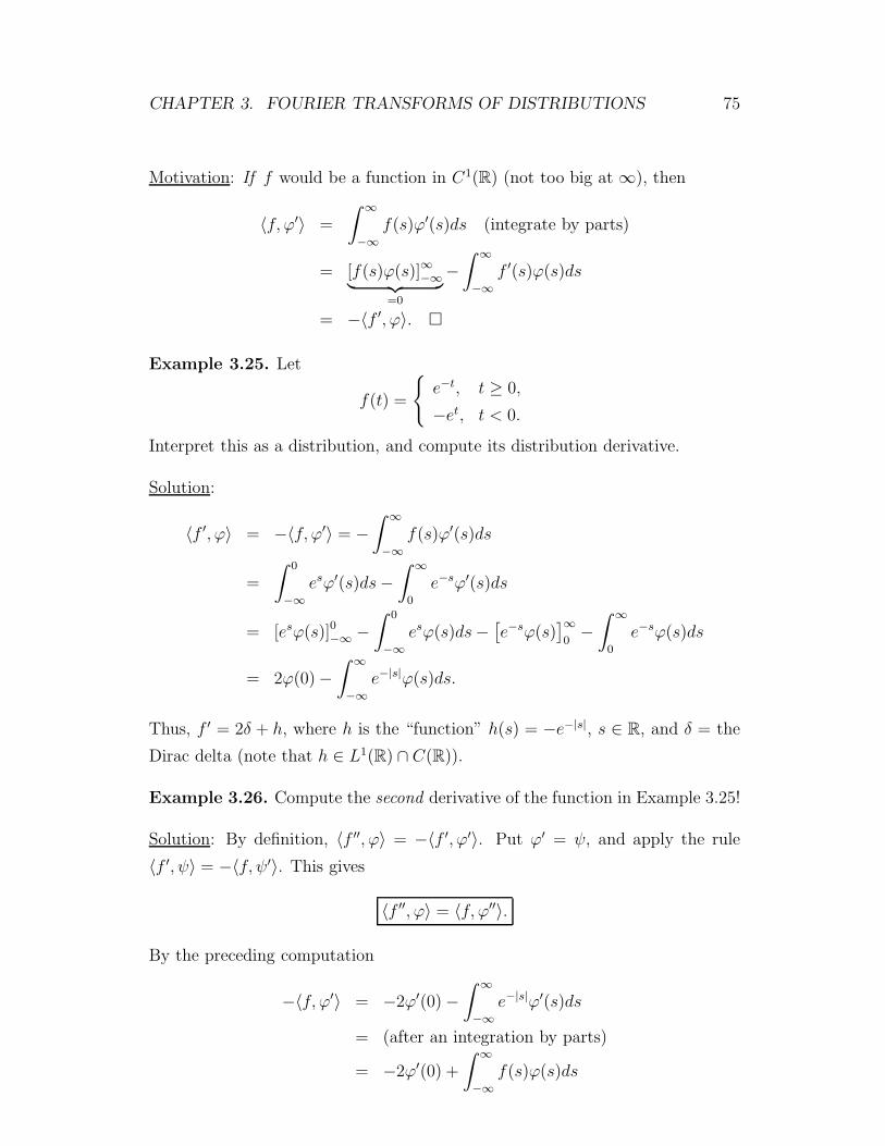
CHAPTER 3. FOURIER TRANSFORMS OF DISTRIBUTIONS 75
Motivation: If f would be a function in C1(R) (not too big at ∞), then
〈f, ϕ′〉 =
∫ ∞
−∞f(s)ϕ′(s)ds (integrate by parts)
= [f(s)ϕ(s)]∞−∞︸ ︷︷ ︸=0
−∫ ∞
−∞f ′(s)ϕ(s)ds
= −〈f ′, ϕ〉.
Example 3.25. Let
f(t) =
e−t, t ≥ 0,
−et, t < 0.
Interpret this as a distribution, and compute its distribution derivative.
Solution:
〈f ′, ϕ〉 = −〈f, ϕ′〉 = −∫ ∞
−∞f(s)ϕ′(s)ds
=
∫ 0
−∞esϕ′(s)ds−
∫ ∞
0
e−sϕ′(s)ds
= [esϕ(s)]0−∞ −∫ 0
−∞esϕ(s)ds−
[e−sϕ(s)
]∞0−∫ ∞
0
e−sϕ(s)ds
= 2ϕ(0) −∫ ∞
−∞e−|s|ϕ(s)ds.
Thus, f ′ = 2δ + h, where h is the “function” h(s) = −e−|s|, s ∈ R, and δ = the
Dirac delta (note that h ∈ L1(R) ∩ C(R)).
Example 3.26. Compute the second derivative of the function in Example 3.25!
Solution: By definition, 〈f ′′, ϕ〉 = −〈f ′, ϕ′〉. Put ϕ′ = ψ, and apply the rule
〈f ′, ψ〉 = −〈f, ψ′〉. This gives
〈f ′′, ϕ〉 = 〈f, ϕ′′〉.
By the preceding computation
−〈f, ϕ′〉 = −2ϕ′(0) −∫ ∞
−∞e−|s|ϕ′(s)ds
= (after an integration by parts)
= −2ϕ′(0) +
∫ ∞
−∞f(s)ϕ(s)ds

CHAPTER 3. FOURIER TRANSFORMS OF DISTRIBUTIONS 76
(f = original function). Thus,
〈f ′′, ϕ〉 = −2ϕ′(0) +
∫ ∞
−∞f(s)ϕ(s)ds.
Conclusion: In the distribution sense,
f ′′ = 2δ′ + f,
where 〈δ′, ϕ〉 = −ϕ′(0). This is the distribution derivative of Dirac’s delta. In
particular: f is a distribution solution of the differential equation
f ′′ − f = 2δ′.
This has something to do with the differential equation on page 59. More about
this later.
3.5 The Fourier Transform of a Distribution
Repetition: By Lemma 2.19, we have
∫ ∞
−∞f(t)g(t)dt =
∫ ∞
−∞f(t)g(t)dt
if f, g ∈ L1(R). Take g = ϕ ∈ S. Then ϕ ∈ S (See Theorem 2.24), so we can
interpret both f and f in the distribution sense and get
Definition 3.27. The Fourier transform of a distribution f ∈ S is the distribu-
tion defined by
〈f , ϕ〉 = 〈f, ϕ〉, ϕ ∈ S.
Possible, since ϕ ∈ S ⇐⇒ ϕ ∈ S.
Problem: Is this really a distribution? It is well-defined and linear, but is it
continuous? To prove this we need to know that
ϕn → ϕ in S ⇐⇒ ϕn → ϕ in S.
This is a true statement (see Gripenberg or Gasquet for a proof), and we get
Theorem 3.28. The Fourier transform maps the class of tempered distributions
onto itself:
f ∈ S ′ ⇐⇒ f ∈ S ′.
CHAPTER 3. FOURIER TRANSFORMS OF DISTRIBUTIONS 77
There is an obvious way of computing the inverse Fourier transform:
Theorem 3.29. The inverse Fourier transform f of a distribution f ∈ S ′ is
given by
〈f, ϕ〉 = 〈f , ψ〉, ϕ ∈ S,
where ψ = the inverse Fourier transform of ϕ, i.e., ψ(t) =∫∞−∞ e2πitωϕ(ω)dω.
Proof. If ψ = the inverse Fourier transform of ϕ, then ϕ = ψ and the formula
simply says that 〈f, ψ〉 = 〈f , ψ〉.
3.6 The Fourier Transform of a Derivative
Problem 3.30. Let f ∈ S ′. Then f ′ ∈ S ′. Find the Fourier transform of f ′.
Solution: Define η(t) = 2πit, t ∈ R. Then η ∈ C∞pol, so we can multiply a
tempered distribution by η. By various definitions (start with 3.27)
〈(f ′), ϕ〉 = 〈f ′, ϕ〉 (use Definition 3.24)
= −〈f, (ϕ)′〉 (use Theorem 2.7(g))
= −〈f, ψ〉 (where ψ(s) = −2πisϕ(s))
= −〈f , ψ〉 (by Definition 3.27)
= 〈f , ηϕ〉 (see Definition above of η)
= 〈ηf , ϕ〉 (by Definition 3.23).
Thus, (f ′) = ηf where η(ω) = 2πiω, ω ∈ R.
This proves one half of:
Theorem 3.31.
(f ′) = (i2πω)f and
(−2πitf) = (f)′
More precisely, if we define η(t) = 2πit, then η ∈ C∞pol, and
(f ′) = ηf , (ηf) = −f ′.
By repeating this result several times we get
Theorem 3.32.
(f (k)) = (2πiω)kf k ∈ Z+
( (−2πit)kf) = f (k).
CHAPTER 3. FOURIER TRANSFORMS OF DISTRIBUTIONS 78
Example 3.33. Compute the Fourier transform of
f(t) =
e−t, t > 0,
−et, t < 0.
Smart solution: By the Examples 3.25 and 3.26.
f ′′ = 2δ′ + f (in the distribution sense).
Transform this:
[(2πiω)2 − 1]f = 2(δ′) = 2(2πiω)δ
(since δ′ is the derivative of δ). Thus, we need δ:
〈δ, ϕ〉 = 〈δ, ϕ〉 = ϕ(0) =
∫
R
ϕ(s)ds
=
∫
R
1 · ϕ(s)ds =
∫
R
f(s)ϕ(s)ds,
where f(s) ≡ 1. Thus δ is the distribution which is induced by the function
f(s) ≡ 1, i.e., we may write δ ≡ 1 .
Thus, −(4π2ω2 + 1)f = 4πiω, so f is induced by the function 4πiω−(1+4π2ω2)
. Thus,
f(ω) =4πiω
−(1 + 4π2ω2).
In particular:
Lemma 3.34.
δ(ω) ≡ 1 and
1 = δ.
(The Fourier transform of δ is the function ≡ 1, and the Fourier transform of
the function ≡ 1 is the Dirac delta.)
Combining this with Theorem 3.32 we get
Lemma 3.35.
δ(k) = (2πiω)k, k ∈ Z+ = 0, 1, 2, . . .[(−2πit)k
]= δ(k)
CHAPTER 3. FOURIER TRANSFORMS OF DISTRIBUTIONS 79
3.7 Convolutions (”Faltningar”)
It is sometimes (but not always) possible to define the convolution of two distri-
butions. One possibility is the following: If ϕ, ψ ∈ S, then we know that
(ϕ ∗ ψ) = ϕψ,
so we can define ϕ ∗ψ to be the inverse Fourier transform of ϕψ. The same idea
applies to distributions in some cases:
Definition 3.36. Let f ∈ S ′ and suppose that g ∈ S ′ happens to be such that
g ∈ C∞pol(R) (i.e., g is induced by a function in C∞
pol(R), i.e., g is the inverse
F -transform of a function in C∞pol). Then we define
f ∗ g = the inverse Fourier transform of f g,
i.e. (cf. page 77):
〈f ∗ g, ϕ〉 = 〈f g, ϕ〉
where ϕ is the inverse Fourier transform of ϕ:
ϕ(t) =
∫ ∞
−∞e2πiωtϕ(ω)dω.
This is possible since g ∈ C∞pol, so that f g ∈ S ′; see page 74
To get a direct interpretation (which does not involve Fourier transforms) we
need two more definitions:
Definition 3.37. Let t ∈ R, f ∈ S ′, ϕ ∈ S. Then the translations τtfand τtϕ
are given by
(τtϕ)(s) = ϕ(s− t), s ∈ R
〈τtf, ϕ〉 = 〈f, τ−tϕ〉
Motivation: τtϕ translates ϕ to the right by the amount t (if t > 0, to the left if
t < 0).
For ordinary functions f we have∫ ∞
−∞(τtf)(s)ϕ(s)ds =
∫ ∞
−∞f(s− t)ϕ(s)ds (s− t = v)
=
∫ ∞
−∞f(v)ϕ(v + t)dv
=
∫ ∞
−∞f(v)τ−tϕ(v)dv,
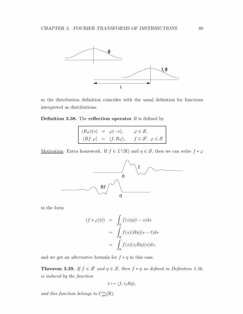
CHAPTER 3. FOURIER TRANSFORMS OF DISTRIBUTIONS 80
t
τ ϕt
ϕ
so the distribution definition coincides with the usual definition for functions
interpreted as distributions.
Definition 3.38. The reflection operator R is defined by
(Rϕ)(s) = ϕ(−s), ϕ ∈ S,〈Rf, ϕ〉 = 〈f, Rϕ〉, f ∈ S ′, ϕ ∈ S
Motivation: Extra homework. If f ∈ L1(R) and η ∈ S, then we can write f ∗ ϕ
0
0
f
Rf
in the form
(f ∗ ϕ)(t) =
∫
R
f(s)η(t− s)ds
=
∫
R
f(s)(Rη)(s− t)ds
=
∫
R
f(s)(τtRη)(s)ds,
and we get an alternative formula for f ∗ η in this case.
Theorem 3.39. If f ∈ S ′ and η ∈ S, then f ∗ η as defined in Definition 3.36,
is induced by the function
t 7→ 〈f, τtRη〉,
and this function belongs to C∞pol(R).
CHAPTER 3. FOURIER TRANSFORMS OF DISTRIBUTIONS 81
We shall give a partial proof of this theorem (skipping the most complicated
part). It is based on some auxiliary results which will be used later, too.
Lemma 3.40. Let ϕ ∈ S, and let
ϕε(t) =ϕ(t+ ε) − ϕ(t)
ε, t ∈ R.
Then ϕε → ϕ′ in S as ε→ 0.
Proof. (Outline) Must show that
limε→0
supt∈R
|t|k|ϕ(m)ε (t) − ϕ(m+1)(t)| = 0
for all t,m ∈ Z+. By the mean value theorem,
ϕ(m)(t+ ε) = ϕ(m)(t) + εϕ(m+1)(ξ)
where t < ξ < t+ ε (if ε > 0). Thus
|ϕ(m)ε (t) − ϕ(m+1)(t)| = |ϕ(m+1)(ξ) − ϕ(m+1)(t)|
= |∫ t
ξ
ϕ(m+2)(s)ds|(
where t < ξ < t+ ε if ε > 0
or t+ ε < ξ < t if ε < 0
)
≤∫ t+|ε|
t−|ε||ϕ(m+2)(s)|ds,
and this multiplied by |t|k tends uniformly to zero as ε→ 0. (Here I am skipping
a couple of lines).
Lemma 3.41. For every f ∈ S ′ there exist two numbers M > 0 and N ∈ Z+ so
that
|〈f, ϕ〉| ≤M max0≤j,k≤Nt∈R
|tjϕ(k)(t)|. (3.2)
Interpretation: Every f ∈ S ′ has a finite order (we need only derivatives ϕ(k)
where k ≤ N) and a finite polynomial growth rate (we need only a finite power
tj with j ≤ N).
Proof. Assume to get a contradiction that (3.2) is false. Then for all n ∈ Z+,
there is a function ϕn ∈ S so that
|〈f, ϕn〉| ≥ n max0≤j,k≤nt∈R
|tjϕ(k)n (t)|.

CHAPTER 3. FOURIER TRANSFORMS OF DISTRIBUTIONS 82
Multiply ϕn by a constant to make 〈f, ϕn〉 = 1. Then
max0≤j,k≤nt∈R
|tjϕ(k)n (t)| ≤ 1
n→ 0 as n→ ∞,
so ϕn → 0 in S as n → ∞. As f is continuous, this implies that 〈f, ϕn〉 → 0
as n → ∞. This contradicts the assumption 〈f, ϕn〉 = 1. Thus, (3.2) cannot be
false.
Theorem 3.42. Define ϕ(t) = 〈f, τtRη〉. Then ϕ ∈ C∞pol, and for all n ∈ Z+,
ϕ(n)(t) = 〈f (n), τtRη〉 = 〈f, τtRη(n)〉.
Note: As soon as we have proved Theorem 3.39, we may write this as
(f ∗ η)(n) = f (n) ∗ η = f ∗ η(n).
Thus, to differentiate f ∗η it suffices to differentiate either f or η (but not both).
The derivatives may also be distributed between f and η:
(f ∗ η)(n) = f (k) ∗ η(n−k), 0 ≤ k ≤ n.
Motivation: A formal differentiation of
(f ∗ ϕ)(t) =
∫
R
f(t− s)ϕ(s)ds gives
(f ∗ ϕ)′ =
∫
R
f ′(t− s)ϕ(s)ds = f ′ ∗ ϕ,
and a formal differentiation of
(f ∗ ϕ)(t) =
∫
R
f(s)ϕ(t− s)ds gives
(f ∗ ϕ)′ =
∫
R
f(s)ϕ′(t− s)ds = f ∗ ϕ′.
Proof of Theorem 3.42.
i) 1ε[ϕ(t+ ε) − ϕ(t)] = 〈f, 1
ε(τt+εRη − τtRη)〉. Here
1
ε(τt+εRη − τtRη)(s) =
1
ε[(Rη)(s− t− ε) − Rη(s− t)]
=1
ε[η(t+ ε− s) − η(t− s)] (by Lemma 3.40)
→ η′(t− s) = (Rη′)(s− t) = τtRη′.
CHAPTER 3. FOURIER TRANSFORMS OF DISTRIBUTIONS 83
Thus, the following limit exists:
limε→0
1
ε[ϕ(t+ ε) − ϕ(t)] = 〈f, τtRη′〉.
Repeating the same argument n times we find that ϕ is n times differen-
tiable, and that
ϕ(n) = 〈f, τtRη(n)〉
(or written differently, (f ∗ η)(n) = f ∗ η(n).)
ii) A direct computation shows: If we put
ψ(s) = η(t− s) = (Rη)(s− t) = (τtRη)(s),
then ψ′(s) = −η′(t − s) = −τtRη′. Thus 〈f, τtRη′〉 = −〈f, ψ′〉 = 〈f ′, ψ〉 =
〈f ′, τtRη〉 (by the definition of distributed derivative). Thus, ϕ′ = 〈f, τtRη′〉 =
〈f ′, τtRη〉 (or written differently, f ∗ η′ = f ′ ∗ η). Repeating this n times
we get
f ∗ η(n) = f (n) ∗ η.
iii) The estimate which shows that ϕ ∈ C∞pol: By Lemma 3.41,
|ϕ(n)(t)| = |〈f (n), τtRη〉|≤ M max
0≤j,k≤Ns∈R
|sj(τtRη)(k)(s)| (ψ as above)
= M max0≤j,k≤Ns∈R
|sjη(k)(t− s)| (t− s = v)
= M max0≤j,k≤Nv∈R
|(t− v)jη(k)(s)|
≤ a polynomial in |t|.
To prove Theorem 3.39 it suffices to prove the following lemma (if two distribu-
tions have the same Fourier transform, then they are equal):
Lemma 3.43. Define ϕ(t) = 〈f, τtRη〉. Then ϕ = f η.
Proof. (Outline) By the distribution definition of ϕ:
〈ϕ, ψ〉 = 〈ϕ, ψ〉 for all ψ ∈ S.

CHAPTER 3. FOURIER TRANSFORMS OF DISTRIBUTIONS 84
We compute this:
〈ϕ, ψ〉 =
∫ ∞
−∞ϕ(s)︸︷︷︸
functionin C∞
pol
ψ(s)ds
=
∫ ∞
−∞〈f, τsRη〉ψ(s)ds
= (this step is too difficult : To show that we may move
the integral to the other side of f requires more theory
then we have time to present)
= 〈f,∫ ∞
−∞τsRηϕ(s)ds〉 = (⋆)
Here τsRη is the function
(τsRη)(t) = (Rη)(t− s) = η(s− t) = (τtη)(s),
so the integral is∫ ∞
−∞η(s− t)ψ(s)ds =
∫ ∞
−∞(τtη)(s)ψ(s)ds (see page 43)
=
∫ ∞
−∞(τtη)(s)ψ(s)ds (see page 38)
=
∫ ∞
−∞e−2πitsη(s)ψ(s)ds
︸ ︷︷ ︸F-transform of ηψ
(⋆) = 〈f, ηψ〉 = 〈f , ηψ〉= 〈f η, ψ〉. Thus, ϕ = f η.
Using this result it is easy to prove:
Theorem 3.44. Let f ∈ S ′, ϕ, ψ ∈ S. Then
(f ∗ ϕ)︸ ︷︷ ︸in C∞
pol
∗ ψ︸︷︷︸in S
︸ ︷︷ ︸in C∞
pol
= f︸︷︷︸in S′
∗ (ϕ ∗ ψ)︸ ︷︷ ︸in S︸ ︷︷ ︸
in C∞pol
Proof. Take the Fourier transforms:
(f ∗ ϕ)︸ ︷︷ ︸↓f ϕ
∗ ψ︸︷︷︸↓ψ︸ ︷︷ ︸
(f ϕ)ψ
= f︸︷︷︸↓f
∗ (ϕ ∗ ψ)︸ ︷︷ ︸↓ϕψ︸ ︷︷ ︸
f(ϕψ)
.

CHAPTER 3. FOURIER TRANSFORMS OF DISTRIBUTIONS 85
The transforms are the same, hence so are the original distributions (note that
both (f ∗ϕ) ∗ψ and f ∗ (ϕ ∗ψ) are in C∞pol so we are allowed to take distribution
Fourier transforms).
3.8 Convergence in S ′
We define convergence in S ′ by means of test functions in S. (This is a special
case of “weak” or “weak*”-convergence).
Definition 3.45. fn → f in S ′ means that
〈fn, ϕ〉 → 〈f, ϕ〉 for all ϕ ∈ S.
Lemma 3.46. Let η ∈ S with η(0) = 1, and define ηλ(t) = λη(λt), t ∈ R, λ > 0.
Then, for all ϕ ∈ S,
ηλ ∗ ϕ→ ϕ in S as λ→ ∞.
Note: We had this type of ”δ-sequences” also in the L1-theory on page 36.
Proof. (Outline.) The Fourier transform is continuous S → S (which we have
not proved, but it is true). Therefore
ηλ ∗ ϕ→ ϕ in S ⇐⇒ ηλ ∗ ϕ→ ϕ in S⇐⇒ ηλϕ→ ϕ in S⇐⇒ η(ω/λ)ϕ(ω) → ϕ(ω) in S as λ→ ∞.
Thus, we must show that
supω∈R
∣∣∣ωk(d
dω
)j[η(ω/λ) − 1]ϕ(ω)
∣∣∣→ 0 as λ→ ∞.
This is a “straightforward” mechanical computation (which does take some time).
Theorem 3.47. Define ηλ as in Lemma 3.46. Then
ηλ → δ in S ′ as λ→ ∞.
Comment: This is the reason for the name ”δ-sequence”.
Proof. The claim (=”pastaende”) is that for all ϕ ∈ S,∫
R
ηλ(t)ϕ(t)dt→ 〈δ, ϕ〉 = ϕ(0) as λ→ ∞.
CHAPTER 3. FOURIER TRANSFORMS OF DISTRIBUTIONS 86
(Or equivalently,∫Rλη(λt)ϕ(t)dt→ ϕ(0) as λ→ ∞). Rewrite this as
∫
R
ηλ(t)(Rϕ)(−t)dt = (ηλ ∗Rϕ)(0),
and by Lemma 3.46, this tends to (Rϕ)(0) = ϕ(0) as λ→ ∞. Thus,
〈ηλ, ϕ〉 → 〈δ, ϕ〉 for all ϕ ∈ S as λ→ ∞,
so ηλ → δ in S ′.
Theorem 3.48. Define ηλ as in Lemma 3.46. Then, for all f ∈ S ′, we have
ηλ ∗ f → f in S ′ as λ→ ∞.
Proof. The claim is that
〈ηλ ∗ f, ϕ〉 → 〈f, ϕ〉 for all ϕ ∈ S.
Replace ϕ with the reflected
ψ = Rϕ =⇒ 〈ηλ ∗ f, Rψ〉 → 〈f, Rψ〉 for all ϕ ∈ S⇐⇒ (by Thm 3.39) ((ηλ ∗ f) ∗ ψ)(0) → (f ∗ ψ)(0) (use Thm 3.44)
⇐⇒ f ∗ (ηλ ∗ ψ)(0) → (f ∗ ψ)(0) (use Thm 3.39)
⇐⇒ 〈f, R(ηλ ∗ ψ)〉 → 〈f, Rψ〉.
This is true because f is continuous and ηλ ∗ ψ → ψ in S, according to Lemma
3.46.
There is a General Rule about distributions:
Metatheorem: All reasonable claims about distribution convergence are true.
Problem: What is “reasonable”?
Among others, the following results are reasonable:
Theorem 3.49. All the operations on distributions and test functions which we
have defined are continuous. Thus, if
fn → f in S ′, gn → g in S ′,
ψn → ψ in C∞pol (which we have not defined!),
ϕn → ϕ in S,λn → λ in C, then, among others,

CHAPTER 3. FOURIER TRANSFORMS OF DISTRIBUTIONS 87
i) fn + gn → f + g in S ′
ii) λnfn → λf in S ′
iii) ψnfn → ψf in S ′
iv) ψn ∗ fn → ψ ∗ f in S ′ (ψ =inverse F-transform of ψ)
v) ϕn ∗ fn → ϕ ∗ f in C∞pol
vi) f ′n → f ′ in S ′
vii) fn → f in S ′ etc.
Proof. “Easy” but long.
3.9 Distribution Solutions of ODE:s
Example 3.50. Find the function u ∈ L2(R+) ∩ C1(R+) with an “absolutely
continuous” derivative u′ which satisfies the equation
u′′(x) − u(x) = f(x), x > 0,
u(0) = 1.
Here f ∈ L2(R+) is given.
Solution. Let v be the solution of homework 22. Thenv′′(x) − v(x) = f(x), x > 0,
v(0) = 0.(3.3)
Define w = u− v. Then w is a solution ofw′′(x) − w(x) = 0, x ≥ 0,
w(0) = 1.(3.4)
In addition we require w ∈ L2(R+).
Elementary solution. The characteristic equation is
λ2 − 1 = 0, roots λ = ±1,
general solution
w(x) = c1ex + c2e
−x.

CHAPTER 3. FOURIER TRANSFORMS OF DISTRIBUTIONS 88
The condition w(x) ∈ L2(R+) forces c1 = 0. The condition w(0) = 1 gives
w(0) = c2e0 = c2 = 1. Thus: w(x) = e−x, x ≥ 0.
Original solution: u(x) = e−x + v(x), where v is a solution of homework 22, i.e.,
u(x) = e−x +1
2e−x
∫ ∞
0
e−yf(y)dy − 1
2
∫ ∞
0
e−|x−y|f(y)dy.
Distribution solution. Make w an even function, and differentiate: we
denote the distribution derivatives by w(1) and w(2). Then
w(1) = w′ (since w is continuous at zero)
w(2) = w′′ + 2w′(0)︸ ︷︷ ︸due to jumpdiscontinuityat zero in w′
δ0 (Dirac delta at the point zero)
The problem says: w′′ = w, so
w(2) − w = 2w′(0)δ0. Transform:
((2πiγ)2 − 1)w(γ) = 2w′(0) (since δ0 ≡ 1)
=⇒ w(γ) = 2w′(0)1+4π2γ2 ,
whose inverse transform is −w′(0)e−|x| (see page 62). We are only interested in
values x ≥ 0 so
w(x) = −w′(0)e−x, x > 0.
The condition w(0) = 1 gives −w′(0) = 1, so
w(x) = e−x, x ≥ 0.
Example 3.51. Solve the equation
u′′(x) − u(x) = f(x), x > 0,
u′(0) = a,
where a =given constant, f(x) given function.
Many different ways exist to attack this problem:
Method 1. Split u in two parts: u = v + w, where
v′′(x) − v(x) = f(x), x > 0
v′(0) = 0,
CHAPTER 3. FOURIER TRANSFORMS OF DISTRIBUTIONS 89
and w′′(x) − w(x) = 0, x > 0
w′(0) = a,
We can solve the first equation by making an even extension of v. The second
equation can be solved as above.
Method 2. Make an even extension of u and transform. Let u(1) and u(2) be
the distribution derivatives of u. Then as above,
u(1) = u′ (u is continuous)
u(2) = u′′ + 2 u′(0)︸︷︷︸=a
δ0 (u′ discontinuous)
By the equation: u′′ = u+ f , so
u(2) − u = 2aδ0 + f
Transform this:[(2πiγ)2 − 1]u = 2a+ f , so
u = −2a1+4π2γ2 − f
1+4π2γ2
Invert:
u(x) = −ae−|x| − 1
2
∫ ∞
−∞e−|x−y|f(y)dy.
Since f is even, this becomes for x > 0:
u(x) = −ae−x − 1
2e−x
∫ ∞
0
e−yf(y)dy − 1
2
∫ ∞
0
e−|x−y|f(y)dy.
Method 3. The method to make u and f even or odd works, but it is a “dirty
trick” which has to be memorized. A simpler method is to define u(t) ≡ 0 and
f(t) ≡ 0 for t < 0, and to continue as above. We shall return to this method in
connection with the Laplace transform.
Partial Differential Equations are solved in a similar manner. The computations
become slightly more complicated, and the motivations become much more com-
plicated. For example, we can replace all the functions in the examples on page
63 and 64 by distributions, and the results “stay the same”.
3.10 The Support and Spectrum of a Distribu-
tion
“Support” = “the piece of the real line on which the distribution stands”
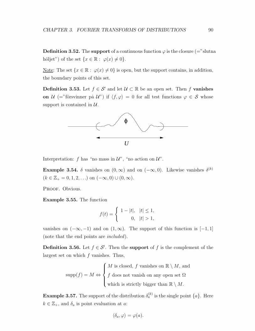
CHAPTER 3. FOURIER TRANSFORMS OF DISTRIBUTIONS 90
Definition 3.52. The support of a continuous function ϕ is the closure (=”slutna
holjet”) of the set x ∈ R : ϕ(x) 6= 0.
Note: The set x ∈ R : ϕ(x) 6= 0 is open, but the support contains, in addition,
the boundary points of this set.
Definition 3.53. Let f ∈ S ′ and let U ⊂ R be an open set. Then f vanishes
on U (=”forsvinner pa U”) if 〈f, ϕ〉 = 0 for all test functions ϕ ∈ S whose
support is contained in U .
U
ϕ
Interpretation: f has “no mass in U”, “no action on U”.
Example 3.54. δ vanishes on (0,∞) and on (−∞, 0). Likewise vanishes δ(k)
(k ∈ Z+ = 0, 1, 2, . . .) on (−∞, 0) ∪ (0,∞).
Proof. Obvious.
Example 3.55. The function
f(t) =
1 − |t|, |t| ≤ 1,
0, |t| > 1,
vanishes on (−∞,−1) and on (1,∞). The support of this function is [−1, 1]
(note that the end points are included).
Definition 3.56. Let f ∈ S ′. Then the support of f is the complement of the
largest set on which f vanishes. Thus,
supp(f) = M ⇔
M is closed, f vanishes on R \M , and
f does not vanish on any open set Ω
which is strictly bigger than R \M .
Example 3.57. The support of the distribution δ(k)a is the single point a. Here
k ∈ Z+, and δa is point evaluation at a:
〈δa, ϕ〉 = ϕ(a).
CHAPTER 3. FOURIER TRANSFORMS OF DISTRIBUTIONS 91
Definition 3.58. The spectrum of a distribution f ∈ S ′ is the support of f .
Lemma 3.59. If M ⊂ R is closed, then supp(f) ⊂M if and only if f vanishes
on R \M .
Proof. Easy.
Example 3.60. Interpret f(t) = tn as a distribution. Then f = 1(−2πi)n δ
(n), as
we saw on page 78. Thus the support of f is 0, so the spectrum of f is 0.
By adding such functions we get:
Theorem 3.61. The spectrum of the function f(t) ≡ 0 is empty. The spectrum
of every other polynomial is the single point 0.
Proof. f(t) ≡ 0 ⇐⇒ spectrum is empty follows from definition. The other
half is proved above.
The converse is true, but much harder to prove:
Theorem 3.62. If f ∈ S ′ and if the spectrum of f is 0, then f is a polynomial
( 6≡ 0).
This follows from the following theorem by taking Fourier transforms:
Theorem 3.63. If the support of f is one single point a then f can be written
as a finite sum
f =
n∑
k=0
anδ(k)a .
Proof. Too difficult to include. See e.g., Rudin’s “Functional Analysis”.
Possible homework: Show that
Theorem 3.64. The spectrum of f is a ⇐⇒ f(t) = e2πiatP (t), where P is a
polynomial, P 6≡ 0.
Theorem 3.65. Suppose that f ∈ S ′ has a bounded support, i.e., f vanishes on
(−∞,−T ) and on (T,∞) for some T > 0 ( ⇐⇒ supp(f) ⊂ [−T, T ]). Then f
can be interpreted as a function, namely as
f(ω) = 〈f, η(t)e−2πiωt〉,
where η ∈ S is an arbitrary function satifying η(t) ≡ 1 for t ∈ [−T−1, T+1] (or,
more generally, for t ∈ U where U is an open set containing supp(f)). Moreover,
f ∈ C∞pol(R).
CHAPTER 3. FOURIER TRANSFORMS OF DISTRIBUTIONS 92
Proof. (Not quite complete)
Step 1. Define
ψ(ω) = 〈f, η(t)e−2πiωt〉,
where η is as above. If we choose two different η1 and η2, then η1(t) − η2(t) = 0
is an open set U containing supp(f). Since f vanishes on R\U , we have
〈f, η1(t)e−2πiωt〉 = 〈f, η2(t)e
−2πiωt〉,
so ψ(ω) does not depend on how we choose η.
Step 2. For simplicity, choose η(t) so that η(t) ≡ 0 for |t| > T + 1 (where T as
in the theorem). A “simple” but boring computation shows that
1
ε[e−2πi(ω+ε)t − e−2πiωt]η(t) → ∂
∂ωe−2πiωtη(t) = −2πite−2πiωtη(t)
in S as ε → 0 (all derivatives converge uniformly on [−T−1, T+1], and everything
is ≡ 0 outside this interval). Since we have convergence in S, also the following
limit exists:
limε→0
1
ε(ψ(ω + ε) − ψ(ω)) = ψ′(ω)
= limε→0
〈f, 1ε(e−2πi(ω+ε)t − e−2πiωt)η(t)〉
= 〈f,−2πite−2πiωtη(t)〉.
Repeating the same computation with η replaced by (−2πit)η(t), etc., we find
that ψ is infinitely many times differentiable, and that
ψ(k)(ω) = 〈f, (−2πit)ke−2πiωtη(t)〉, k ∈ Z+. (3.5)
Step 3. Show that the derivatives grow at most polynomially. By Lemma 3.41,
we have
|〈f, ϕ〉| ≤M max0≤t,l≤Nt∈R
|tjϕ(l)(t)|.
Apply this to (3.5) =⇒
|ψ(k)(ω)| ≤ M max0≤j,l≤Nt∈R
∣∣∣tj(d
dt
)l(−2πit)ke−2πiωtη(t)
∣∣∣.
The derivative l = 0 gives a constant independent of ω.
The derivative l = 1 gives a constant times |ω|.
CHAPTER 3. FOURIER TRANSFORMS OF DISTRIBUTIONS 93
The derivative l = 2 gives a constant times |ω|2, etc.
Thus, |ψ(k)(ω)| ≤ const. x[1 + |w|N ], so ψ ∈ C∞pol.
Step 4. Show that ψ = f . That is, show that∫
R
ψ(ω)ϕ(ω)dω = 〈f , ϕ〉(= 〈f, ϕ〉).
Here we need the same “advanced” step as on page 83:∫
R
ψ(ω)ϕ(ω)dω =
∫
R
〈f, e−2πiωtη(t)ϕ(ω)〉dω
= (why??) = 〈f,∫
R
e−2πiωtη(t)ϕ(ω)dω〉
= 〈f, η(t)ϕ(t)〉(
since η(t) ≡ 1 in a
neighborhood of supp(f)
)
= 〈f, ϕ〉.
A very short explanation of why “why??” is permitted: Replace the integral by
a Riemann sum, which converges in S, i.e., approximate
∫
R
e−2πiωtϕ(ω)dω = limn→∞
∞∑
k=−∞e−2πiωktϕ(ωk)
1
n,
where ωk = k/n.
3.11 Trigonometric Polynomials
Definition 3.66. A trigonometric polynomial is a sum of the form
ψ(t) =m∑
j=1
cje2πiωjt.
The numbers ωj are called the frequencies of ψ.
Theorem 3.67. If we interpret ψ as a polynomial then the spectrum of ψ is
ω1, ω2, . . . , ωm, i.e., the spectrum consists of the frequencies of the polynomial.
Proof. Follows from homework 27, since supp(δωj) = ωj.
Example 3.68. Find the spectrum of the Weierstrass function
σ(t) =∞∑
k=0
ak cos(2πbkt),
where 0 < a < 1, ab ≥ 1.

CHAPTER 3. FOURIER TRANSFORMS OF DISTRIBUTIONS 94
To solve this we need the following lemma
Lemma 3.69. Let 0 < a < 1, b > 0. Then
N∑
k=0
ak cos(2πbkt) →∞∑
k=0
ak cos(2πbkt)
in S ′ as N → ∞.
Proof. Easy. Must show that for all ϕ ∈ S,
∫
R
(N∑
k=0
−∞∑
k=0
)ak cos(2πbkt)ϕ(t)dt→ 0 as N → ∞.
This is true because
∫
R
∞∑
k=N+1
|ak cos(2πbkt)ϕ(t)|dt ≤∫
R
∞∑
k=N+1
ak|ϕ(t)|dt
≤∞∑
k=N+1
ak∫ ∞
−∞|ϕ(t)|dt
=aN+1
1 − a
∫ ∞
−∞|ϕ(t)|dt→ 0 as N → ∞.
Solution of 3.68: Since∑N
k=0 →∑∞
k=0 in S ′, also the Fourier transforms converge
in S ′, so to find σ it is enough to find the transform of∑N
k=0 ak cos(2πbkt) and
to let N → ∞. This transform is
δ0 +1
2[a(δb + δ−b) + a2(δ−b2 + δb2) + . . .+ aN (δ−bN + δbN )].
Thus,
σ = δ0 +1
2
∞∑
n=1
an(δ−bn + δbn),
where the sum converges in S ′, and the support of this is 0,±b,±b2,±b3, . . .,which is also the spectrum of σ.
Example 3.70. Let f be periodic with period 1, and suppose that f ∈ L1(T),
i.e.,∫ 1
0|f(t)|dt <∞. Find the Fourier transform and the spectrum of f .
Solution: (Outline) The inversion formula for the periodic transform says that
f =
∞∑
n=−∞f(n)e2πint.
CHAPTER 3. FOURIER TRANSFORMS OF DISTRIBUTIONS 95
Working as on page 86 (but a little bit harder) we find that the sum converges
in S ′, so we are allowed to take transforms:
f =
∞∑
n=−∞f(n)δn (converges still in S ′).
Thus, the spectrum of f is n ∈ N : f(n) 6= 0. Compare this to the theory of
Fourier series.
General Conclusion 3.71. The distribution Fourier transform contains all the
other Fourier transforms in this course. A “universal transform”.
3.12 Singular differential equations
Definition 3.72. A linear differential equation of the type
n∑
k=0
aku(k) = f (3.6)
is regular if it has exactly one solution u ∈ S ′ for every f ∈ S ′. Otherwise it is
singular.
Thus: Singular means: For some f ∈ S ′ it has either no solution or more than
one solution.
Example 3.73. The equation u′ = f . Taking f = 0 we get many different so-
lutions, namely u =constant (different constants give different solutions). Thus,
this equation is singular.
Example 3.74. We saw earlier on page 59-63 that if we work with L2-functions
instead of distributions, then the equation
u′′ + λu = f
is singular iff λ > 0. The same result is true for distributions:
Theorem 3.75. The equation (3.6) is regular
⇔n∑
k=0
ak(2πiω)k 6= 0 for all ω ∈ R.
CHAPTER 3. FOURIER TRANSFORMS OF DISTRIBUTIONS 96
Before proving this, let us define
Definition 3.76. The function D(ω) =∑n
k=0 ak(2πiω)k is called the symbol of
(3.6)
Thus: Singular ⇔ the symbol vanishes for some ω ∈ R.
Proof of theorem 3.75. Part 1: Suppose that D(ω) 6= 0 for all ω ∈ R.
Transform (3.6):
n∑
k=0
ak(2πiω)ku = f ⇔ D(ω)u = f .
If D(ω) 6= 0 for all ω, then 1D(ω)
∈ C∞pol, so we can multiply by 1
D(ω):
u =1
D(ω)f ⇔ u = K ∗ f
where K is the inverse distribution Fourier transform of 1D(ω)
. Therefore, (3.6)
has exactly one solution u ∈ S ′ for every f ∈ S ′.
Part 2: Suppose that D(a) = 0 for some a ∈ R. Then
〈Dδa, ϕ〉 = 〈δa, Dϕ〉 = D(a)ϕ(a) = 0.
This is true for all ϕ ∈ S, so Dδa is the zero distribution: Dδa = 0.
⇔n∑
k=0
ak(2πiω)kδa = 0.
Let v be the inverse transform of δa, i.e.,
v(t) = e2πiat ⇒n∑
k=0
akv(k) = 0.
Thus, v is one solution of (3.6) with f ≡ 0. Another solution is v ≡ 0. Thus,
(3.6) has at least two different solutions ⇒ the equation is singular.
Definition 3.77. If (3.6) is regular, then we call K =inverse transform of 1D(ω)
the Green’s function of (3.6). (Not defined for singular problems.)
How many solutions does a singular equation have? Find them all! (Solution
later!)
CHAPTER 3. FOURIER TRANSFORMS OF DISTRIBUTIONS 97
Example 3.78. If f ∈ C(R) (and |f(t)| ≤M(1 + |t|k) for some M and k), then
the equation
u′ = f
has at least the solutions
u(x) =
∫ x
0
f(x)dx+ constant
Does it have more solutions?
Answer: No! Why?
Suppose that u′ = f and v′ = f ⇒ u′−v′ = 0. Transform this ⇒ (2πiω)(u−v) =
0.
Let ϕ be a test function which vanishes in some interval [−ε, ε](⇔ the support
of ϕ is in (−∞,−ε] ∪ [ε,∞)). Then
ψ(ω) =ϕ(ω)
2πiω
is also a test function (it is ≡ 0 in [−ε, ε]), since (2πiω)(u− v) = 0 we get
0 = 〈(2πiω)(u− v), ψ〉= 〈u− v, 2πiωψ(ω)〉 = 〈u− v, ϕ〉.
Thus, 〈u − v, ϕ〉 = 0 when supp(ϕ) ⊂ (−∞,−ε] ∪ [ε,∞), so by definition,
supp(u− v) ⊂ 0. By theorem 3.63, u− v is a polynomial. The only polynomial
whose derivative is zero is the constant function, so u− v is a constant.
A more sophisticated version of the same argument proves the following theorem:
Theorem 3.79. Suppose that the equation
n∑
k=0
aku(k) = f (3.7)
is singular, and suppose that the symbolD(ω) has exactly r simple zeros ω1, ω2, . . . , ωr.
If the equation (3.7) has a solution v, then every other solution u ∈ S ′ of (3.7)
is of the form
u = v +
r∑
j=1
bje2πiωjt,
where the coefficients bj can be chosen arbitrarily.

CHAPTER 3. FOURIER TRANSFORMS OF DISTRIBUTIONS 98
Compare this to example 3.78: The symbol of the equation u′ = f is 2πiω, which
has a simple zero at zero.
Comment 3.80. The equation (3.7) always has a distribution solution, for all
f ∈ S ′. This is proved for the equation u′ = f in [GW99, p. 277], and this can
be extended to the general case.
Comment 3.81. A zero ωj of order r ≥ 2 of D gives rise to terms of the type
P (t)e2πiωjt, where P (t) is a polynomial of degree ≤ r − 1.

Chapter 4
The Fourier Transform of a
Sequence (Discrete Time)
From our earlier results we very quickly get a Fourier transform theory for se-
quences an∞n=−∞. We interpret this sequence as the distribution
∞∑
n=−∞anδn (δn = Dirac’s delta at the point n)
For example, this converges in S ′ if
|an| ≤M(1 + |n|N) for some M,N
and the Fourier transform is:
∞∑
n=−∞ane
−2πiωn =
∞∑
k=−∞a−ke
2πiωk
which also converges in S ′. This transform is identical to the inverse transform
discussed in Chapter 1 (periodic function!), except for the fact that we replace i
by −i (or equivalently, replace n by −n). Therefore:
Theorem 4.1. All the results listed in Chapter 1 can be applied to the theory
of Fourier transforms of sequences, provided that we intercharge the Fourier
transform and the inverse Fourier transform.
Notation 4.2. To simplify the notations we write the original sequence as f(n),
n ∈ Z, and denote the Fourier transform as f . Then f is periodic (function or
99

CHAPTER 4. FOURIER SERIES 100
distribution, depending on the size of |f(n)| as n→ ∞), and
f(ω) =∞∑
n=−∞f(n)e−2πiωn.
From Chapter 1 we can give e.g., the following results:
Theorem 4.3.
i) f ∈ ℓ2(Z) ⇔ f ∈ L2(T),
ii) f ∈ ℓ1(Z) ⇒ f ∈ C(T) (converse false),
iii) (f g) = f ∗ g if e.g.
f ∈ L1(T)
g ∈ L1(T)or
f ∈ ℓ2(Z)
g ∈ ℓ2(Z)
iv) Etc.
We can also define discrete convolutions:
Definition 4.4. (f ∗ g)(n) =∑∞
k=−∞ f(n− k)g(k).
This is defined whenever the sum converges absolutely. For example, if f(k) 6= 0
only for finitely many k or if
f ∈ ℓ1(Z), g ∈ ℓ∞(Z), or if
f ∈ ℓ2(Z), g ∈ ℓ2(Z), etc.
Lemma 4.5.
i) f ∈ ℓ1(Z), g ∈ Lp(Z), 1 ≤ p ≤ ∞, ⇒ f ∗ g ∈ ℓp(Z)
ii) f ∈ ℓ1(Z), g ∈ c0(Z) ⇒ f ∗ g ∈ c0(Z).
Proof. “Same” as in Chapter 1 (replace all integrals by sums).
Theorem 4.6. If f ∈ ℓ1(Z) and g ∈ ℓ1(Z), then
(f ∗ g)(ω) = f(ω)g(ω).
Also true if e.g. f ∈ ℓ2(Z) and g ∈ ℓ2(Z).
Proof. ℓ1-case: “Same” as proof of Theorem 1.21 (replace integrals by sums).
In the ℓ2-case we first approximate by an ℓ1-sequence, use the ℓ1-theory, and pass
to the limit.
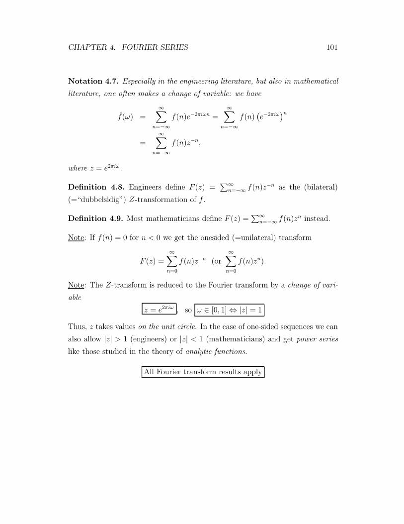
CHAPTER 4. FOURIER SERIES 101
Notation 4.7. Especially in the engineering literature, but also in mathematical
literature, one often makes a change of variable: we have
f(ω) =
∞∑
n=−∞f(n)e−2πiωn =
∞∑
n=−∞f(n)
(e−2πiω
)n
=∞∑
n=−∞f(n)z−n,
where z = e2πiω.
Definition 4.8. Engineers define F (z) =∑∞
n=−∞ f(n)z−n as the (bilateral)
(=“dubbelsidig”) Z-transformation of f .
Definition 4.9. Most mathematicians define F (z) =∑∞
n=−∞ f(n)zn instead.
Note: If f(n) = 0 for n < 0 we get the onesided (=unilateral) transform
F (z) =
∞∑
n=0
f(n)z−n (or
∞∑
n=0
f(n)zn).
Note: The Z-transform is reduced to the Fourier transform by a change of vari-
able
z = e2πiω , so ω ∈ [0, 1] ⇔ |z| = 1
Thus, z takes values on the unit circle. In the case of one-sided sequences we can
also allow |z| > 1 (engineers) or |z| < 1 (mathematicians) and get power series
like those studied in the theory of analytic functions.
All Fourier transform results apply
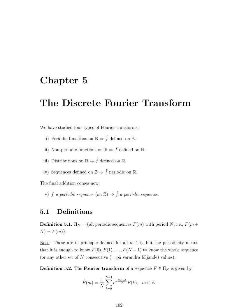
Chapter 5
The Discrete Fourier Transform
We have studied four types of Fourier transforms:
i) Periodic functions on R ⇒ f defined on Z.
ii) Non-periodic functions on R ⇒ f defined on R.
iii) Distributions on R ⇒ f defined on R.
iv) Sequences defined on Z ⇒ f periodic on R.
The final addition comes now:
v) f a periodic sequence (on Z) ⇒ f a periodic sequence.
5.1 Definitions
Definition 5.1. ΠN = all periodic sequences F (m) with period N , i.e., F (m+
N) = F (m).
Note: These are in principle defined for all n ∈ Z, but the periodicity means
that it is enough to know F (0), F (1), . . . , F (N − 1) to know the whole sequence
(or any other set of N consecutive (= pa varandra foljande) values).
Definition 5.2. The Fourier transform of a sequence F ∈ ΠN is given by
F (m) =1
N
N−1∑
k=0
e−2πimk
N F (k), m ∈ Z.
102
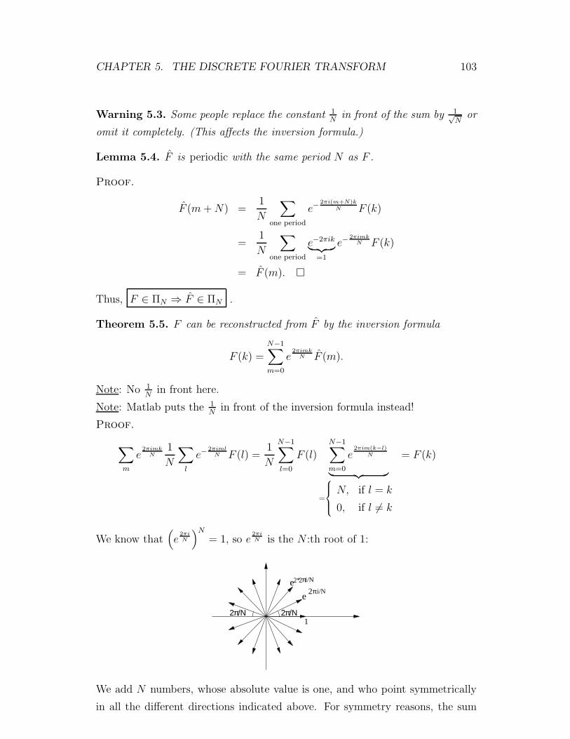
CHAPTER 5. THE DISCRETE FOURIER TRANSFORM 103
Warning 5.3. Some people replace the constant 1N
in front of the sum by 1√N
or
omit it completely. (This affects the inversion formula.)
Lemma 5.4. F is periodic with the same period N as F .
Proof.
F (m+N) =1
N
∑
one period
e−2πi(m+N)k
N F (k)
=1
N
∑
one period
e−2πik︸ ︷︷ ︸
=1
e−2πimk
N F (k)
= F (m).
Thus, F ∈ ΠN ⇒ F ∈ ΠN .
Theorem 5.5. F can be reconstructed from F by the inversion formula
F (k) =
N−1∑
m=0
e2πimk
N F (m).
Note: No 1N
in front here.
Note: Matlab puts the 1N
in front of the inversion formula instead!
Proof.
∑
m
e2πimk
N1
N
∑
l
e−2πiml
N F (l) =1
N
N−1∑
l=0
F (l)
N−1∑
m=0
e2πim(k−l)
N
︸ ︷︷ ︸
=
8
>
>
<
>
>
:
N, if l = k
0, if l 6= k
= F (k)
We know that(e
2πiN
)N= 1, so e
2πiN is the N :th root of 1:
2πi/Ne
e2*2πi/N
2π/Ν 2π/Ν1
We add N numbers, whose absolute value is one, and who point symmetrically
in all the different directions indicated above. For symmetry reasons, the sum

CHAPTER 5. THE DISCRETE FOURIER TRANSFORM 104
must be zero (except when l = k). (You always jump an angle 2π(k−l)N
for each
turn, and go k − l times around before you are done.)
Definition 5.6. The convolution F ∗G of two sequences in ΠN are defined by
(F ∗G)(m) =∑
one period
F (m− k)G(k)
(Note: Some indeces get out of the interval [0, N−1]. You must use the periodicity
of F and G to get the corresponding values of F (m− k)G(k).).
Definition 5.7. The (ordinary) product F ·G is defined by
(F ·G)(m) = F (m)G(m), m ∈ Z.
Theorem 5.8. (F ·G) = F ∗ G and (F ∗G) = NF · G (note the extra factor
N).
Proof. Easy. (Homework?)
Definition 5.9. (RF )(n) = F (−n) (reflection operator).
As before: The inverse transform = the ususal transform plus reflection:
Theorem 5.10. F = N(RF ) (note the extra factor N), where ˆ = Fourier
transform and ˇ= Inverse Fourier transform.
Proof. Easy. We could have avoided the factor N by a different scaling (but
then it shows up in other places instead).
5.2 FFT=the Fast Fourier Transform
Question 5.11. How many flops do we need to compute the Fourier transform
of F ∈ ΠN?
FLOP=FLoating Point Operation=multiplication or addition or combination
of both.
1 Megaflop = 1 million flops/second (106)
1 Gigaflop = 1 billion flops/second (109)
(Used as speed measures of computers.)
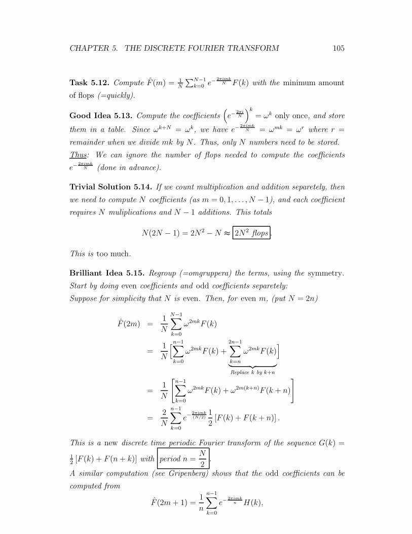
CHAPTER 5. THE DISCRETE FOURIER TRANSFORM 105
Task 5.12. Compute F (m) = 1N
∑N−1k=0 e
− 2πimkN F (k) with the minimum amount
of flops (=quickly).
Good Idea 5.13. Compute the coefficients(e−
2πiN
)k= ωk only once, and store
them in a table. Since ωk+N = ωk, we have e−2πimk
N = ωmk = ωr where r =
remainder when we divide mk by N . Thus, only N numbers need to be stored.
Thus: We can ignore the number of flops needed to compute the coefficients
e−2πimk
N (done in advance).
Trivial Solution 5.14. If we count multiplication and addition separetely, then
we need to compute N coefficients (as m = 0, 1, . . . , N − 1), and each coefficient
requires N muliplications and N − 1 additions. This totals
N(2N − 1) = 2N2 −N ≈ 2N2 flops .
This is too much.
Brilliant Idea 5.15. Regroup (=omgruppera) the terms, using the symmetry.
Start by doing even coefficients and odd coefficients separetely:
Suppose for simplicity that N is even. Then, for even m, (put N = 2n)
F (2m) =1
N
N−1∑
k=0
ω2mkF (k)
=1
N
[n−1∑
k=0
ω2mkF (k) +
2n−1∑
k=n
ω2mkF (k)
︸ ︷︷ ︸Replace k by k+n
]
=1
N
[n−1∑
k=0
ω2mkF (k) + ω2m(k+n)F (k + n)
]
=2
N
n−1∑
k=0
e−2πimk(N/2)
1
2[F (k) + F (k + n)] .
This is a new discrete time periodic Fourier transform of the sequence G(k) =
12[F (k) + F (n+ k)] with period n =
N
2.
A similar computation (see Gripenberg) shows that the odd coefficients can be
computed from
F (2m+ 1) =1
n
n−1∑
k=0
e−2πimk
n H(k),
CHAPTER 5. THE DISCRETE FOURIER TRANSFORM 106
where H(k) = 12e−
iπkn [F (k) − F (k + n)]. Thus, instead of one transform of order
N we get two transforms of order n = N2.
Number of flops: Computing the new transforms by brute force (as in 5.14 on
page 105) we need the following flops:
Even: n(2n− 1) = N2
2− N
2+ n additions = N2
2flops.
Odd: The numbers e−iπkn = e−
2iπkN are found in the table already computed.
We essentially again need the same amount, namely N2
2+ N
2(n extra multiplica-
tions).
Total: N2
2+ N2
2+ N
2= N2+ N
2≈ N2. Thus, this approximately halfed the number
of needed flops.
Repeat 5.16. Divide the new smaller transforms into two halfs, and again, and
again. This is possible if N = 2k for some integer k, e.g., N = 1024 = 210.
Final conclusion: After some smaller adjustments we get down to
3
22kk flops.
Here N = 2k, so k = log2N , and we get
Theorem 5.17. The Fast Fourier Transform with radius 2 outlined above needs
approximately 32N log2N flops.
This is much smaller than 2N2 − N for large N . For example N = 210 = 1024
gives3
2N log2N ≈ 15000 ≪ 2000000 = 2N2 −N.
Definition 5.18. Fast Fourier transform with
radius 2 : split into 2 parts at each step N = 2k
radius 3 : split into 3 parts at each step N = 3k
radius m : split into m parts at each step N = mk
Note: Based on symmetries. “The same” computations repeat themselves, so by
combining them in a clever way we can do it quicker.
Note: The FFT is so fast that it caused a minor revolution to many branches of
numerical analysis. It made it possible to compute Fourier transforms in practice.
Rest of this chapter: How to use the FFT to compute the other transforms dis-
cussed earlier.

CHAPTER 5. THE DISCRETE FOURIER TRANSFORM 107
5.3 Computation of the Fourier Coefficients of
a Periodic Function
Problem 5.19. Let f ∈ C(T). Compute
f(k) =
∫ 1
0
e−2πiktf(t)dt
as efficiently as possible.
Solution: Turn f into a periodic sequence and use FFT!
Conversion 5.20. Choose some N ∈ Z, and put
F (m) = f(m
N), m ∈ Z
(equidistant “sampling”). The periodicity of f makes F periodic with period N .
Thus, F ∈ ΠN .
Theorem 5.21 (Error estimte). If f ∈ C(T) and f ∈ ℓ1(Z) (i.e.,∑
|f(k)| <∞),
then
F (m) − f(m) =∑
k 6=0
f(m+ kN).
Proof. By the inversion formula, for all t,
f(t) =∑
j∈Z
e2πijtf(j).
Put tk = kN
⇒f(tk) = F (k) =
∑
j∈Z
e2πikj
N f(j)
(this series converges uniformly by Lemma 1.14). By the definition of F :
F (m) =1
N
N−1∑
k=0
e−2πimk
N F (k)
=1
N
∑
j∈Z
f(j)N−1∑
k=0
e2πi(j−m)k
N
︸ ︷︷ ︸
=
8
>
>
<
>
>
:
N, if j−mN
= integer
0, if j−mN
6= integer
=∑
l∈Z
f(m+Nl).
CHAPTER 5. THE DISCRETE FOURIER TRANSFORM 108
Take away the term f(m) (l = 0) to get
F (m) = f(m) +∑
l 6=0
f(m+Nl).
Note: If N is “large” and if f(m) → 0 “quickly” as m→ ∞, then the error
∑
l 6=0
f(m+Nl) ≈ 0.
First Method 5.22. Put
i) f(m) ≈ F (m) if |m| < N2
ii) f(m) ≈ 12F (m) if |m| = N
2(N even)
iii) f(m) ≈ 0 if |m| > N2.
Here ii) is not important. We could use f(N2) = 0 or f(N
2) = F (m) instead.
Here
F (m) =1
N
N−1∑
k=0
e−2πimk
N F (k).
Notation 5.23. Let us denote (note the extra star)
∗∑
|k|≤N/2ak =
∑
|k|≤N/2ak
= the usual sum of ak if N odd (then we have exactly N terms), and
∗∑
|k|≤N/2ak =
a sum where the first and last terms have been
divided by two (these are the same if the sequence
is periodic with period N , there is “one term too
many” in this case).
First Method 5.24 (Error). The first method gives the error:
i) |m| < N2
gives the error
|f(m) − F (m)| ≤∑
k 6=0
|f(m+ kN)|
ii) |m| = N2
gives the error
|f(m) − 1
2F (m)|
CHAPTER 5. THE DISCRETE FOURIER TRANSFORM 109
iii) |m| > N2
gives the error |f(m)|.
we can simplify this into the following crude (=”grov”) estimate:
supm∈Z
|f(m) − F (m)| ≤∗∑
|m|≥N/2|f(m)| (5.1)
(because this sum is ≥ the actual error).
First Method 5.25 (Drawbacks).
1 Large error.
2 Inaccurate error estimate (5.1).
3 The error estimate based on f and not on f .
We need a better method.
Second Method 5.26 (General Principle).
1 Evaluate t at the points tk = kN
(as before), F (k) = f(tk)
2 Use the sequence F to construct a new function P ∈ C(T ) which “approx-
imates” f .
3 Compute the Fourier coefficients of P .
4 Approximate f(n) by P (n).
For this to succeed we must choose P in a smart way. The final result will be
quite simple, but for later use we shall derive P from some “basic principles”.
Choice of P 5.27. Clearly P depends on F . To simplify the computations we
require P to satisfy (write P = P (F ))
A) P is linear: P (λF + µG) = λP (F ) + µP (G)
B) P is translation invariant: If we translate F , then P (F ) is translated by
the same amount: If we denote
(τjF )(m) = F (m− j), then
P (τjF ) = τj/NP (F )
(j discrete steps ⇐⇒ a time difference of j/N).

CHAPTER 5. THE DISCRETE FOURIER TRANSFORM 110
This leads to simple computations: We want to compute P (m) (which we use as
approximations of f(m)) Define a δ-sequence:
D(n) =
1, for n = 0,±N,±2N, . . .
0, otherwise.
Then
N 2Nperiod
zero
(τkD)(n) =
1, if n = k + jN, j ∈ Z
0, otherwise,
so
[F (k)τkD](n) =
F (k), n = k + jN
0, otherwise.
and so
F =
N−1∑
k=0
F (k)τkD
Therefore, the principles A) and B) give
P (F ) =
N−1∑
k=0
F (k)P (τkD)
=
N−1∑
k=0
F (k)τk/NP (D),
Where P (D) is the approximation of D = “unit pulse at time zero” D.

CHAPTER 5. THE DISCRETE FOURIER TRANSFORM 111
We denote this function by p. Let us transform P (F ):
(P (F ))(m) =
∫ 1
0
N+1∑
k=0
F (k)(τk/Np)(s)e−2πismds
=
N+1∑
k=0
F (k)
∫ 1
0
e−2πismp(s− k
N)ds (s− k
N= t)
=N+1∑
k=0
F (k)
∫one
period
e−2πim(t+ kN
)p(t)dt
=N+1∑
k=0
F (k)e−−2πimk
N
∫one
period
e−2πimtp(t)dt
︸ ︷︷ ︸p(m)
= p(m)N+1∑
k=0
F (k)e−2πimk
N
︸ ︷︷ ︸=NF (m)
= Np(m)F (m).
We can get rid of the factor N by replacing p by Np. This is our approximation
of the “pulse of size N at zero”
N, n = 0 + jN
0, otherwise.
Second Method 5.28. Construct F as in the First Method, and compute F .
Then the approximation of f(m) is
f(m) ≈ F (m)p(m),
where p is the Fourier transform of the function that we get when we apply our
approximation procedure to the sequence
ND(n) =
N, n = 0(+jN)
0, otherwise.
Note: The complicated proof of this simple method will pay off in a second!
Approximation Method 5.29. Use any type of translation-invariant inter-
polation method, for example splines. The simplest possible method is linear
interpolation: If we interpolate the pulse ND in this way we get Thus,
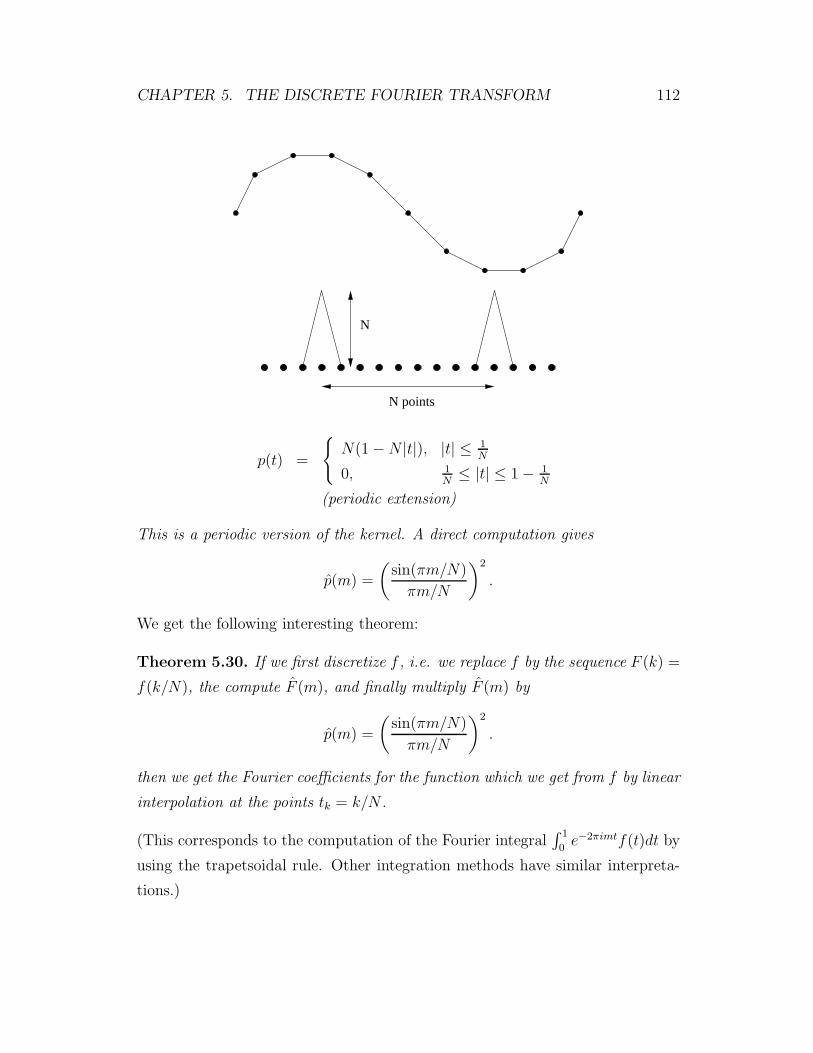
CHAPTER 5. THE DISCRETE FOURIER TRANSFORM 112
N points
N
p(t) =
N(1 −N |t|), |t| ≤ 1
N
0, 1N
≤ |t| ≤ 1 − 1N
(periodic extension)
This is a periodic version of the kernel. A direct computation gives
p(m) =
(sin(πm/N)
πm/N
)2
.
We get the following interesting theorem:
Theorem 5.30. If we first discretize f , i.e. we replace f by the sequence F (k) =
f(k/N), the compute F (m), and finally multiply F (m) by
p(m) =
(sin(πm/N)
πm/N
)2
.
then we get the Fourier coefficients for the function which we get from f by linear
interpolation at the points tk = k/N .
(This corresponds to the computation of the Fourier integral∫ 1
0e−2πimtf(t)dt by
using the trapetsoidal rule. Other integration methods have similar interpreta-
tions.)
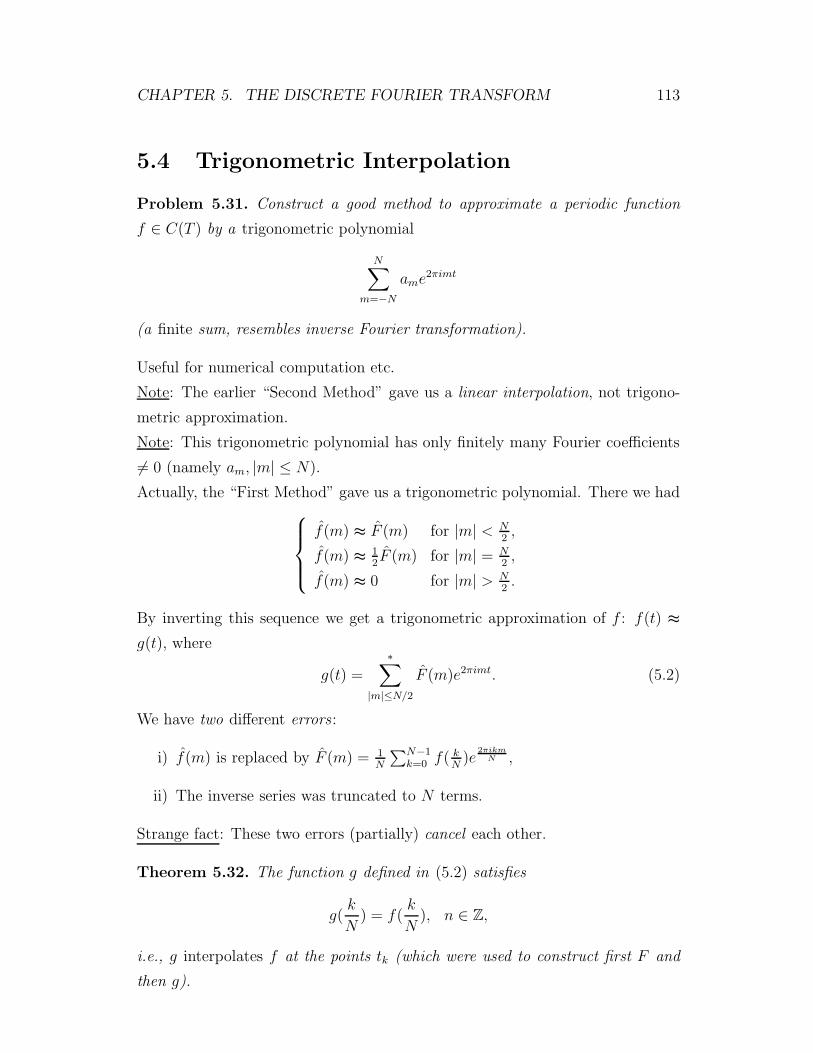
CHAPTER 5. THE DISCRETE FOURIER TRANSFORM 113
5.4 Trigonometric Interpolation
Problem 5.31. Construct a good method to approximate a periodic function
f ∈ C(T ) by a trigonometric polynomial
N∑
m=−Name
2πimt
(a finite sum, resembles inverse Fourier transformation).
Useful for numerical computation etc.
Note: The earlier “Second Method” gave us a linear interpolation, not trigono-
metric approximation.
Note: This trigonometric polynomial has only finitely many Fourier coefficients
6= 0 (namely am, |m| ≤ N).
Actually, the “First Method” gave us a trigonometric polynomial. There we had
f(m) ≈ F (m) for |m| < N2,
f(m) ≈ 12F (m) for |m| = N
2,
f(m) ≈ 0 for |m| > N2.
By inverting this sequence we get a trigonometric approximation of f : f(t) ≈
g(t), where
g(t) =
∗∑
|m|≤N/2F (m)e2πimt. (5.2)
We have two different errors:
i) f(m) is replaced by F (m) = 1N
∑N−1k=0 f( k
N)e
2πikmN ,
ii) The inverse series was truncated to N terms.
Strange fact: These two errors (partially) cancel each other.
Theorem 5.32. The function g defined in (5.2) satisfies
g(k
N) = f(
k
N), n ∈ Z,
i.e., g interpolates f at the points tk (which were used to construct first F and
then g).
CHAPTER 5. THE DISCRETE FOURIER TRANSFORM 114
Proof. We defined F (k) = f( kN
), and
F (m) =∗∑
|k|≤N/2F (k)e−
2πimkN .
By the inversion formula on page 103,
g(k
N) =
∗∑
|m|≤N/2F (m)e
2πimkN (use periodicity)
=
N−1∑
m=0
F (m)e2πimk
N
= F (k) = f(k
N)
Error estimate: How large is |f(t)−g(t)| between the mesh points tk = kN
(where
the error is zero)? We get an estimate from the computation in the last section.
Suppose that f ∈ ℓ1(Z) and f ∈ C(T ) so that the inversion formula holds for all
t (see Theorem 1.37). Then
f(t) =∑
m∈Z
f(m)e2πimt, and
g(t) =∗∑
|m|≤N/2F (m)e2πimt (Theorem 5.21)
=
∗∑
|m|≤N/2
[f(m) +
∑
k 6=0
f(m+ kN)
]e2πimt
= f(t) −∗∑
|m|≥N/2f(m)e2πimt +
∗∑
|m|≤N/2
∑
k 6=0
f(m+ kN)e2πimt.
Thus
|g(t) − f(t)| ≤∗∑
|m|≥N/2|f(m)| +
∗∑
|m|≤N/2
∑
k 6=0
|f(m+ kM)|︸ ︷︷ ︸
=P∗
|l|≥N/2|f(l)|
= 2∗∑
|m|≥N/2|f(m)|
(take l = m + kN , every |l| > N2
appears one time, no |l| < N2
appears, and
|l| = N2
two times).
This leads to the following theorem:
CHAPTER 5. THE DISCRETE FOURIER TRANSFORM 115
Theorem 5.33. If∑∞
m=−∞|f(m)| <∞, then
|g(t) − f(t)| ≤ 2∗∑
|m|≥N/2|f(m)|,
whereg(t) =
∑∗|m|≤N/2 F (m)e2πimt, and
F (m) = 1N
∑∗|m|≤N/2 e
− 2πimkN f( k
N).
This is nice if f(m) → 0 rapidly as m→ ∞. Better accuracy by increasing N .
5.5 Generating Functions
Definition 5.34. The generating function of the sequence Jn(x) is the func-
tion
f(x, z) =∑
n
Jn(x)zn,
where the sum over n ∈ Z or over n ∈ Z+, depending on for which values of n
the functions Jn(x) are defined.
Note: We did this in the course on special functions. E.g., if Jn = Bessel’s
function of order n, then
f(x, z) = ex2(z−1/2).
Note: For a fixed value of x, this is the “mathematician’s version” of the Z-
transform described on page 101.
Make a change of variable:
z = e2πit ⇒ f(x, e2πit) =∑
n∈Z
Jn(x)(e2πit)n
=∑
n∈Z
Jn(x)e2πint,
Comparing this to the inversion formula in Chapter 1 we get
Theorem 5.35. For a fixed x, the n:th Fourier coefficient of the function t 7→f(x, e2πit) is equal to Jn(x).
Thus, we can compute Jn(x) by the method descibed in Section 5.3 to compute
the coefficients an = Jn(x) (x = fixed, n varies):

CHAPTER 5. THE DISCRETE FOURIER TRANSFORM 116
1) Discretize F (k) = f(x, e2πik
N )
2) F (m) = 1N
∑∗|k|≤N/2 e
− 2πimkN F (k)
3) F (m) − Jn(x) =∑
k 6=0 am+kN , (Theorem 5.21)
where am+kN = Jm+kN(x).
5.6 One-Sided Sequences
So far we have been talking about periodic sequences (in ΠN). Instead one often
wants to discuss
A) Finite sequences A(0), A(1), . . . , A(N − 1) or
B) One-sided sequences A(n), n ∈ Z+ = 0, 1, 2 . . .
Note: 5.36. A finite sequence is a special csse of a one-sided sequence: put
A(n) = 0 for n ≥ N .
Note: 5.37. A one-sided sequence is a special case of a two-sided sequence: put
A(n) = 0 for n < 0.
Problem: These extended sequences are not periodic. ⇒ We cannot use the Fast
Fourier Transform directly.
Notation 5.38. CZ+ = all complex valued sequences A(n), n ∈ Z+
Definition 5.39. The convolution of two sequences A,B ∈ CZ+ is
(A ∗B)(m) =
m∑
k=0
A(m− k)B(k), m ∈ Z+
Note: The summation boundaries are the natural ones if we think that A(k) =
B(k) = 0 for k < 0.
Notation 5.40.
A|n(k) =
A(k), 0 ≤ k < n
0, k ≥ n.
Thus, this restricts the sequence A(k) to the n first terms.

CHAPTER 5. THE DISCRETE FOURIER TRANSFORM 117
Lemma 5.41. (A ∗B)|n = (A|n ∗B|n)|n
Proof. Easy.
Notation 5.42. A = 0n means that A(k) = 0 for 0 ≤ k < n− 1, i.e., A|n = 0.
Lemma 5.43. If A = 0n and B = 0m, then A ∗B = 0n+m.
Proof. Easy.
Computation of A ∗B 5.44 (One-sided convolution).
1) Choose a number N ≥ 2n (often a power of 2).
2) Define
F (k) =
A(k), 0 ≤ k < n,
0, n ≤ k < N,
and extend F to be periodic, period N .
3) Define
G(k) =
B(k), 0 ≤ k < n,
0, n ≤ k < N,
periodic extension: G(k +N) = G(k).
Then, for all m, 0 ≤ m < n,
(F ∗G)(m)︸ ︷︷ ︸periodic convolution
=
N−1∑
k=0
F (m− k)G(k)
=
m∑
k=0
F (m− k)G(k)
=m∑
k=0
A(m− k)G(k) = (A ∗B)(m)︸ ︷︷ ︸one-sided convolution
Note: Important that N ≥ 2n.
Thus, this way we have computed the n first coefficients of (A ∗B).
Theorem 5.45. The method described below allows us to compute (A ∗ B)|n
(=the first n coefficients of A ∗B) with a number of FLOP:s which is
C · n log2 n, where C is a constant.
Method: 1)-3) same as above

CHAPTER 5. THE DISCRETE FOURIER TRANSFORM 118
4) Use FFT to compute
F · G(= N(F ∗G)).
5) Use the inverse FFT to compute
F ∗G =1
N(F · G)
Then (A ∗B)|n = (F ∗G)|n.
Note: A “naive” computation of A ∗ B|n requires C1 · n2 FLOPs, where C1 is
another constant.
Note: Use “naive” method if n small. Use “FFT-inverse FFT” if n is large.
Note: The rest of this chapter applies one-sided convolutions to different situa-
tions. In all cases the method described in Theorem 5.45 can be used to compute
these.
5.7 The Polynomial Interpretation of a Finite
Sequence
Problem 5.46. Compute the product of two polynomials:
p(x) =
n∑
k=0
akxk q(x) =
m∑
l=0
blxl.
Solution: Define ak = 0 for k > 0 and bl = 0 for l > m. Then
p(x)q(x) =
( ∞∑
k=0
akxk
)( ∞∑
l=0
blxl
)
︸ ︷︷ ︸sums are actually finite
=∑
k,l
akblxk+l (k + l = j, k = j − l)
=∑
j
xjj∑
l=0
aj−lbl =m+n∑
j=0
cjxj ,
where cj =∑j
l=0 aj−lbl. This gives
Theorem 5.47.

CHAPTER 5. THE DISCRETE FOURIER TRANSFORM 119
i) Multiplication of two polynomials corresponds to a convolution of their
coefficients: If
p(x) =
n∑
k=0
akxk, q(x) =
m∑
l=0
blxl,
then p(x)q(x) =∑m+n
j=0 cjxj, where c = a ∗ b.
ii) Addition of two polynomials corresponds to addition of the coefficients:
p(x) + q(x) =∑
cjxj , where cj = aj + bj .
iii) Multiplication of a polynomial by a complex constant corresponds to mul-
tiplication of the coefficients by the same constant.
Operation Polynomial Coefficients
Addition p(x) + q(x) ak + bkmaxm,nk=0
Multiplication by
λ ∈ C
λp(x) λaknk=0
Multiplication p(x)q(x) (a ∗ b)(k)Thus there is a one-to-one correspondence between
polynomials ⇐⇒ finite sequences,
where the operations correspond as described above. This is used in all symbolic
computer computations of polynomials.
Note: Two different conventions are in common use:
A) first coefficient is a0 (= lowest order),
B) first coefficient is an (= highest order).
5.8 Formal Power Series and Analytic Functions
Next we extend “polynomials” so that they may contain infinitely many terms.
Definition 5.48. A Formal Power Series (FPS) is a sum of the type
∞∑
k=0
A(k)xk
which need not converge for any x 6= 0. (If it does converge, then it defines an
analytic function in the region of convergence.)

CHAPTER 5. THE DISCRETE FOURIER TRANSFORM 120
Example 5.49.∑∞
k=0xk
k!converges for all x (and the sum is ex).
Example 5.50.∑∞
k=0 xk converges for |x| < 1 (and the sum is 1
1−x).
Example 5.51.∑∞
k=0 k!xk converges for no x 6= 0.
All of these are formal power series (and the first two are “ordinary” power
series).
Calculus with FPS 5.52. We borrow the calculus rules from the polynomials:
i) We add two FPS:s by adding the coefficients:
[ ∞∑
k=0
A(k)xk
]+
[ ∞∑
k=0
B(k)xk
]=
∞∑
k=0
[A(k) +B(k)]xk.
ii) We multiply a FPS by a constant λ by multiplying each coefficients by λ:
λ
∞∑
k=0
A(k)xk =
∞∑
k=0
[λA(k)]xk.
iii) We multiply two FPS:s with each other by taking the convolution of the
coefficients:
[ ∞∑
k=0
A(k)xk
][ ∞∑
k=0
B(k)xk
]=
∞∑
k=0
C(k)xk,
where C = A ∗B.
Notation 5.53. We denote A(x) =∑∞
k=0A(k)xk.
Conclusion 5.54. There is a one-to-one correspondence between all Formal
Power Series and all one-sided sequences (bounded or not). We denoted these by
CZ+ on page 116.
Comment 5.55. In the sequence (=”fortsattningen”) we operate with FPS:s.
These power series often converge, and then they define analytic functions, but
this fact is not used anywhere in the proofs.

CHAPTER 5. THE DISCRETE FOURIER TRANSFORM 121
5.9 Inversion of (Formal) Power Series
Problem 5.56. Given a (formal) power series A(x) =∑A(k)xk, find the in-
verse formal power series B(x) =∑B(k)xk.
Thus, we want to find B(x) so that
A(x)B(x) = 1, i.e.,[ ∞∑
k=0
A(k)xk
][ ∞∑
l=0
B(l)xl
]= 1 + 0x+ 0x2 + . . .
Notation 5.57. δ0 = 1, 0, 0, . . . = the sequence whose power series is 1 +
0x+ 0x2 + . . .. This series converges, and the sum is ≡ 1. More generally:
δk = 0, 0, 0, . . . , 0, 1, 0, 0, . . .= 0 + 0x+ 0x2 + . . .+ 0xk−1 + 1xk + 0xk+1 + 0xk+2 + . . .
= xk
Power Series Sequence
δk xk
Solution. We know that A∗B = δ0, or equivalently, A(x)B(x) = 1. Explicitly,
A(x)B(x) = A(0)B(0) (times x0) (5.3)
+[A(0)B(1) + A(1)B(0)]x (5.4)
+[A(0)B(2) + A(1)B(1) + A(2)B(0)]x2 (5.5)
+ . . . (5.6)
From this we can solve:
i) A(0)B(0) = 1 =⇒ A(0) 6= 0 and B(0) = 1A(0)
.
ii) A(0)B(1) + A(1)B(0) = 0 =⇒ B(1) = −A(1)B(0)A(0)
(always possible)
iii) A(0)B(2) + A(1)B(1) + A(2)B(0) = 1 =⇒ B(2) = − 1A(0)
[A(1)B(1) +
A(2)B(0)], etc.
we get a theorem:
Theorem 5.58. The FPS A(x) can be inverted if and only if A(0) 6= 0. The
inverse series [A(x)]−1 is obtained recursively by the procedure described above.
CHAPTER 5. THE DISCRETE FOURIER TRANSFORM 122
Recursive means:
i) Solve B(0)
ii) Solve B(1) using B(0)
iii) Solve B(2) using B(1) and B(0)
iv) Solve B(3) using B(2), B(1) and B(0), etc.
This is Hard Work. For example
sin(x) = x− x3
3!+x5
5!− . . .
cos(x) = 1 − x2
2!+x4
4!− . . .
tan(x) =sin(x)
cos(x)= sin(x)
1
cos(x)︸ ︷︷ ︸convolution
=???
Hard Work means: Number of FLOPS is a constant times N2. Better method:
Use FFT.
Theorem 5.59. Let A(0) 6= 0. and let B(x) be the inverse of A(x). Then, for
every k ≥ 1,
B|2k = (B|k ∗ (2δ0 − A ∗B|k))|2k (5.7)
Proof. See Gripenberg.
Usage: First compute B|1 = 1A(0)
, 0, 0, 0, . . .Then B|2 = B(0), B(1), 0, 0, 0, . . . (use (5.7))
Then B|4 = B(0), B(1), B(2), B(3), 0, , 0, 0, . . .Then B|8 = 8 terms 6= 0 etc.
Use the method on page 117 for the convolutions. (Useful only if you need lots
of coefficients).
5.10 Multidimensional FFT
Especially in image processing we also need the discrete Fourier transform in
several dimensions. Let d = 1, 2, 3, . . . be the “space dimension”. Put ΠdN =
sequences x(k1, k2, . . . , kd) which are N -periodic in each variable separately.
CHAPTER 5. THE DISCRETE FOURIER TRANSFORM 123
Definition 5.60. The d-dimensional Fourier transform is obtained by transform-
ing d successive (=”efter varandra”) “ordinary” Fourier transformations, one for
each variable.
Lemma 5.61. The d-dimensional Fourier transform is given by
x(m1, m2, . . . , md) =1
Nd
∑
k1
∑
k2
· · ·∑
kd
e−2πi(k1m1+k2m2+...+kdmd)
N x(k1, k2, . . . , kd).
Proof. Easy.
All 1-dimensional results generalize easy to the d-dimensional case.
Notation 5.62. We call k = (k1, k2, . . . , kd) and m = (m1, m2, . . . , md) multi-
indeces (=pluralis av “multi-index”), and put
k · m = k1m1 + k2m2 + . . .+ kdmd
(=the “inner product” of k and m).
Lemma 5.63.
x(m) =1
Nd
∑
k
e−2πim·k
N x(k),
x(k) =∑
me
2πim·kN x(m).
Definition 5.64.
(F ·G)(m) = F (m)G(m)
(F ∗G)(m) =∑
k
F (m − k)G(k),
where all the components of m and k run over one period.
Theorem 5.65.
(F ·G) = F ∗ G,(F ∗G) = NdF · G.
Proof. Follows from Theorem 5.8.
In practice: Either use one multi-dimensional, or use d one-dimensional trans-
forms (not much difference, multi-dimensional a little faster).
Chapter 6
The Laplace Transform
6.1 General Remarks
Example 6.1. We send in a “signal” u into an “amplifier”, and get an “output
signal” y:
Black boxu y
Under quite general assumptions it can be shown that
y(t) = (K ∗ u)(t) =
∫ t
−∞K(t− s)u(s)ds,
i.e., the output is the convolution (=”faltningen”) of u with the “inpulse re-
sponse” K.
Terminology 6.2. “Impulse response” (=pulssvar) since y = K if u = a delta
distribution.
Causality 6.3. The upper bound in the integral is t, i.e., (K ∗u)(t) depends only
on past values of u, and not on future values. This is called causality.
If, in addition u(t) = 0 for t < 0, then y(t) = 0 for t < 0, and
y(t) =
∫ t
0
K(t− s)u(s)ds,
which is a one-sided convolution.
Classification 6.4. Approximately: The Laplace-transform is the Fourier trans-
form applied to one-sided signals (defined on R+). In addition there is a change
of variable which rotate the complax plane.
124
CHAPTER 6. THE LAPLACE TRANSFORM 125
6.2 The Standard Laplace Transform
Definition 6.5. Suppose that∫∞0e−σt|f(t)|dt < ∞ for some σ ∈ R. Then we
define the Laplace transform f(s) of f by
f(s) =
∫ ∞
0
e−stf(t)dt, ℜ(s) ≥ σ.
Lemma 6.6. The integral above converges absolutely for all s ∈ C with ℜ(s) ≥ σ
(i.e., f(s) is well-defined for such s).
Proof. Write s = α + iβ. Then
|e−stf(t)| = |e−αteiβtf(t)|= e−αt|f(t)|≤ e−σt|f(t)|, so∫ ∞
0
|e−stf(t)|dt ≤∫ ∞
0
e−σt|f(t)|dt <∞.
Theorem 6.7. f(s) is analytic in the open half-plane Re(s) > σ, i.e., f(s) has
a complex derivative with respect to s.
Proof. (Outline)
f(z) − f(s)
z − s=
∫ ∞
0
e−zt − e−st
z − sf(t)dt
=
∫ ∞
0
e−(z−s)t − 1
z − se−stf(t)dt (put z − s = h)
=
∫ ∞
0
1
h[e−ht − 1]︸ ︷︷ ︸→−t as h→0
e−stf(t)dt
As Re(s) > σ we find that∫∞0
|te−stf(t)|d <∞ and a “short”computation (about12
page) shows that the Lebesgue dominated convergence theorem can be applied
(show that | 1h(e−ht − 1)| ≤ const. · t · eαt, where α = 1
2[σ + ℜ(s)] (this is true
for some small enough h), and then show that∫∞0teαt|e−stf(t)|dt < ∞). Thus,
ddsf(s) exists, and
d
dsf(s) = −
∫ ∞
0
e−sttf(t)dt, ℜ(s) > σ
Corollary 6.8. ddsf(s) is the Laplace transform of g(t) = −tf(t), and this
Laplace transform converges (at least) in the half-plane Re(s) > σ.
CHAPTER 6. THE LAPLACE TRANSFORM 126
Theorem 6.9. f(s) is bounded in the half-plane ℜ(s) ≥ σ.
Proof. (cf. proof of Lemma 6.6)
|f(s)| = |∫ ∞
0
e−stf(t)dt| ≤∫ ∞
0
|e−stf(t)|dt
=
∫ ∞
0
e−(ℜs)t|f(t)|dt ≤∫ ∞
0
e−σt|f(t)|dt <∞.
Definition 6.10. A bounded analytic function on the half-plane Re(s) > σ
is called a H∞-function (over this half-plane).
Theorem 6.11. If f is absolutely continuous and∫∞0e−σt|g(t)|dt < ∞ (i.e.,
f(t) = f(0) +∫ t0g(s)ds, where
∫∞0e−σt|g(t)|dt <∞), then
(f ′)(s) = sf(s) − f(0), ℜ(s) > σ.
Proof. Integration by parts (a la Lebesgue) gives
limT→∞
∫ T
0
e−stf(t)
︸ ︷︷ ︸=f(s)
dt = limT→∞
([e−st−s f(t)
]T0
+1
s
∫ ∞
0
e−stf ′(t)dt
)
=1
sf(0) +
1
sf ′(s), so
(f ′)(s) = sf(s) − f(0).
6.3 The Connection with the Fourier Transform
Let Re(s) > σ, and make a change of variable:∫ ∞
0
e−stf(t)dt (t = 2πv; dt = 2πdv)
=
∫ ∞
0
e−2πsvf(2πv)2πdv (s = α + iω)
=
∫ ∞
0
e−2πiωve−2παvf(2πv)2πdv (put f(t) = 0 for t < 0)
=
∫ ∞
−∞e−2πiωtg(t)dt,
where
g(t) =
2πe−2παtf(2πt) , t ≥ 0
0 , t < 0.(6.1)
Thus, we got

CHAPTER 6. THE LAPLACE TRANSFORM 127
Theorem 6.12. On the line Re(s) = α (which is a line parallell with the imagi-
nary axis −∞ < ω < ∞) f(s) coincides (=sammanfaller med) with the Fourier
transform of the function g defined in (6.1).
Thus, modulo a change of variable, the Laplace transform is the Fourier transform
of a function vanishing for t < 0. From Theorem 6.12 and the theory about
Fourier transforms of functions in L1(R) and L2(R) we can derive a number of
results. For example:
Theorem 6.13. (Compare to Theorem 2.3, page 36) If f ∈ L1(R+) (i.e.,∫∞0
|f(t)|dt <∞), then
lim|s|→∞ℜ(s)≥0
|f(s)| = 0
(where s→ ∞ in the half plane Re(s) > 0 in an arbitrary manner)
Re
Im
Combining Theorem 6.12 with one of the theorems about the inversion of the
Fourier integral we get formulas of the type
1
2π
∫ ∞
−∞e2πiωtf(α + iω)dω =
e−2παtf(t), t > 0,
0, t < 0.
This is often written as a complex line integral: We integrate along the line
Re(s) = α, and replace 2πt → t and multiply the formulas by e2παt to get
(s = α + iω, ds = idω)
f(t) =1
2πi
∫ α+i∞
α−i∞estf(s)ds (6.2)
=1
2πi
∫ ∞
ω=−∞e(α+iω)tf(α + iω)idω
CHAPTER 6. THE LAPLACE TRANSFORM 128
Warning 6.14. This integral seldom converges absolutely. If it does converge
absolutely, then (See Theorem 2.3 with the Fourier theorem replaced by the in-
verse Fourier theorem) the function
g(t) =
2πe−2παtf(t), t ≥ 0,
0, t < 0
must be continuous. In other words:
Lemma 6.15. If the integral (6.2) converges absolutely, then f must be contin-
uous and satisfy f(0) = 0.
Therefore, the inversion theorems given in Theorem 2.30 and Theorem 2.31 are
much more useful. They give (under the assumptions given there)
1
2[f(t+) + f(t−)] = lim
T→∞
1
2πi
∫ α+iT
α−iTestf(s)ds
(and we interpret f(t) = 0 for t < 0). By Theorem 6.11, if f is absolutely
continuous and f ′ ∈ L1(R+), then (use also Theorem 6.13)
f(s) =1
s[ ˜(f ′)(s) + f(0)],
where ˜(f ′)(s) → 0 as |s| → ∞, ℜ(s) ≥ 0. Thus, for large values of ω, f(α+iω) ≈f(0)iω
, so the convergence is slow in general. Apart from the space H∞ (see page
126) (over the half plane) another much used space (especially in Control theory)
is H2.
Theorem 6.16. If f ∈ L2(R+), then the Laplace transform f of f is analytic in
the half-plane ℜ(s) > 0, and it satisfy, in addition
supα>0
∫ ∞
−∞|f(α + iω)|2dω <∞,
i.e., there is a constant M so that∫ ∞
−∞|f(α+ iω)|2dω ≤M (for all α > 0).
Proof. By Theorem 6.12 and the L2-theory for Fourier integrals (see Section
2.3),∫ ∞
−∞|f(α + iω)|2dω =
∫ ∞
0
|2πe−2παtf(2πt)|2dt (2πt = v)
= 2π
∫ ∞
0
|e−αvf(v)|2dv
≤ 2π
∫ ∞
0
|f(v)|2dv = 2π‖f‖L2(0,∞).
CHAPTER 6. THE LAPLACE TRANSFORM 129
Converesly:
Theorem 6.17. If ϕ is analytic in ℜ(s) > 0, and ϕ satisfies
supα>0
∫ ∞
−∞|ϕ(α + iω)|2dω <∞, (6.3)
then ϕ is the Laplace transform of a function f ∈ L2(R+).
Proof. Not too difficult (but rather long).
Definition 6.18. An H2-function over the half-plane ℜ(s) > 0 is a function ϕ
which is analytic and satisfies (6.3).
6.4 The Laplace Transform of a Distribution
Let f ∈ S ′ (tempered distribution), and suppose that the support of f is con-
tained in [0,∞) = R+ (i.e., f vanishes on (−∞, 0)). Then we can define the
Laplace transform of f in two ways:
i) Make a change of variables as on page 126 and use the Fourier transform
theory.
ii) Define f(s) as f applied to the “test function” e−st, t > 0. (Warning: this
is not a test function!)
Both methods lead to the same result, but the second method is actually simpler.
If ℜ(s) > 0, then t 7→ e−st behaves like a test function on [0,∞) but not on
(−∞, 0). However, f is supported on [0,∞), so it does not matter how e−st
behaves for t < 0. More precisely, we take an arbitrary “cut off” function
η ∈ C∞pol satisfying
η(t) ≡ 1 for t ≥ −1,
η(t) ≡ 0 for t ≤ −2.
Then η(t)e−st = e−st for t ∈ [−1,∞), and since f is supported on [0,∞) we can
replace e−st by η(t)e−st to get
Definition 6.19. If f ∈ S ′ vanishes on (−∞, 0), then we define the Laplace
transform f(s) of f by
f(s) = 〈f, η(t)e−st〉, ℜ(s) > 0.
CHAPTER 6. THE LAPLACE TRANSFORM 130
(Compare this to what we did on page 84).
Note: In the same way we can define the Laplace transform of a distribution that
is not necessarily tempered, but which becomes tempered after multiplication by
e−σt for some σ > 0. In this case the Laplace transform will be defined in the
half-plane ℜs > σ.
Theorem 6.20. If f vanishes on (−∞, 0), then f is analytic on the half-plane
ℜs > 0.
Proof omitted.
Note: f need not be bounded. For example, if f = δ′, then
(δ′)(s) = 〈δ′, η(t)e−st〉 = −〈δ, η(t)e−st〉
=d
dte−st |t=0 = −s.
(which is unbounded). On the other hand
δ(s) = 〈δ, η(t)e−st〉 = e−st |t=0 = 1.
Theorem 6.21. If f ∈ S ′ vanishes on (−∞, 0), then
i) [tf(t)](s) = −[f(s)]′
ii) f ′(s) = sf(s)
ℜ(s) > 0
Proof. Easy (homework?)
Warning 6.22. You can apply this distribution transform also to functions, but
remember to put f(t) = 0 for t < 0. This automatically leads to a δ-term in the
distribution derivative of f : after we define f(t) = 0 for t < 0, the distribution
derivative of f is
f(0)δ0︸ ︷︷ ︸dervatives of jump at zero
+ f ′(t)︸︷︷︸usual derivative
6.5 Discrete Time: Z-transform
This is a short continuation of the theory on page 101.
In discrete time we also run into one-sided convolutions (as we have seen), and
it is possible to compute these by the FFT. From a mathematical point of view
the Z-tranform is often simpler than the Fourier transform.
CHAPTER 6. THE LAPLACE TRANSFORM 131
Definition 6.23. The Z-transform of a sequence f(n)∞n=0 is given by
f(z) =
∞∑
n=0
f(n)z−n,
for all these z ∈ C for which the series converges absolutely.
Lemma 6.24.
i) There is a number ρ ∈ [0,∞] so that f(z) converges for |z| > ρ and f(z)
diverges for |z| < ρ.
ii) f is analytic for |z| > ρ.
Proof. Course on analytic functions.
As we noticed on page 101, the Z-transform can be converted to the discrete
time Fourier transform by a simple change of variable.
6.6 Using Laguerra Functions and FFT to Com-
pute Laplace Transforms
We start by recalling some results from the course in special functions:
Definition 6.25. The Laguerra polynomials Lm are given by
Lm(t) =1
m!et( ddt
)m(tme−t), m ≥ 0,
and the Laguerra functions ℓm are given by
ℓ,(t) =1
m!e
t2
( ddt
)m(tme−t), m ≥ 0.
Note that ℓm(t) = e−t2Lm(t).
Lemma 6.26. The Laguerra polynomials can be computed recusively from the
formula
(m+ 1)Lm+1(t) + (t− 2m− 1)Lm(t) +mLm−1(t) = 0,
with starting values L−1 ≡ 0 and L1 ≡ 1.
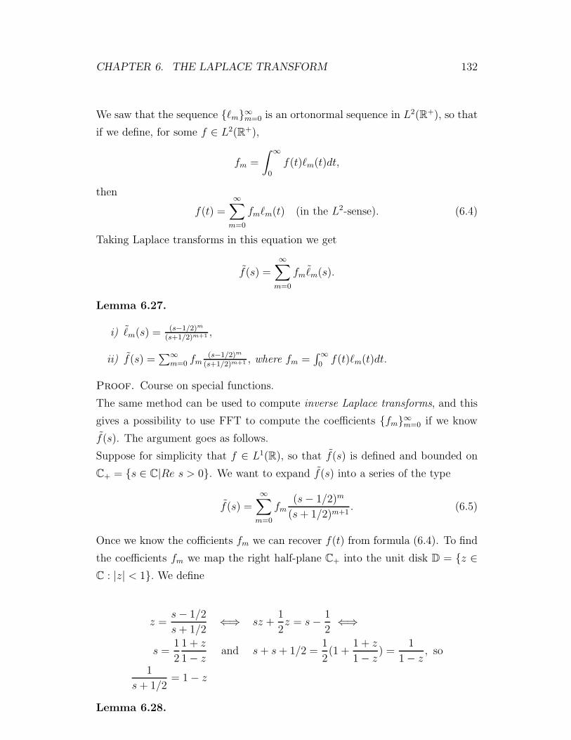
CHAPTER 6. THE LAPLACE TRANSFORM 132
We saw that the sequence ℓm∞m=0 is an ortonormal sequence in L2(R+), so that
if we define, for some f ∈ L2(R+),
fm =
∫ ∞
0
f(t)ℓm(t)dt,
then
f(t) =
∞∑
m=0
fmℓm(t) (in the L2-sense). (6.4)
Taking Laplace transforms in this equation we get
f(s) =
∞∑
m=0
fmℓm(s).
Lemma 6.27.
i) ℓm(s) = (s−1/2)m
(s+1/2)m+1 ,
ii) f(s) =∑∞
m=0 fm(s−1/2)m
(s+1/2)m+1 , where fm =∫∞0f(t)ℓm(t)dt.
Proof. Course on special functions.
The same method can be used to compute inverse Laplace transforms, and this
gives a possibility to use FFT to compute the coefficients fm∞m=0 if we know
f(s). The argument goes as follows.
Suppose for simplicity that f ∈ L1(R), so that f(s) is defined and bounded on
C+ = s ∈ C|Re s > 0. We want to expand f(s) into a series of the type
f(s) =
∞∑
m=0
fm(s− 1/2)m
(s+ 1/2)m+1. (6.5)
Once we know the cofficients fm we can recover f(t) from formula (6.4). To find
the coefficients fm we map the right half-plane C+ into the unit disk D = z ∈C : |z| < 1. We define
z =s− 1/2
s+ 1/2⇐⇒ sz +
1
2z = s− 1
2⇐⇒
s =1
2
1 + z
1 − zand s+ s+ 1/2 =
1
2(1 +
1 + z
1 − z) =
1
1 − z, so
1
s+ 1/2= 1 − z
Lemma 6.28.
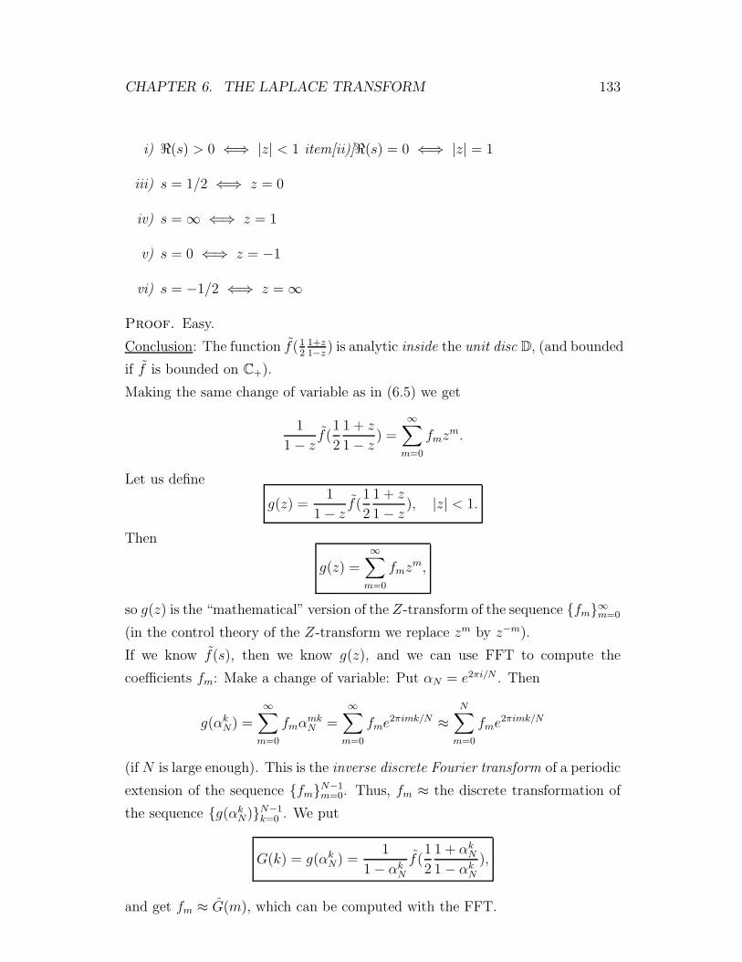
CHAPTER 6. THE LAPLACE TRANSFORM 133
i) ℜ(s) > 0 ⇐⇒ |z| < 1 item[ii)]ℜ(s) = 0 ⇐⇒ |z| = 1
iii) s = 1/2 ⇐⇒ z = 0
iv) s = ∞ ⇐⇒ z = 1
v) s = 0 ⇐⇒ z = −1
vi) s = −1/2 ⇐⇒ z = ∞
Proof. Easy.
Conclusion: The function f(12
1+z1−z ) is analytic inside the unit disc D, (and bounded
if f is bounded on C+).
Making the same change of variable as in (6.5) we get
1
1 − zf(
1
2
1 + z
1 − z) =
∞∑
m=0
fmzm.
Let us define
g(z) =1
1 − zf(
1
2
1 + z
1 − z), |z| < 1.
Then
g(z) =∞∑
m=0
fmzm,
so g(z) is the “mathematical” version of the Z-transform of the sequence fm∞m=0
(in the control theory of the Z-transform we replace zm by z−m).
If we know f(s), then we know g(z), and we can use FFT to compute the
coefficients fm: Make a change of variable: Put αN = e2πi/N . Then
g(αkN) =
∞∑
m=0
fmαmkN =
∞∑
m=0
fme2πimk/N ≈
N∑
m=0
fme2πimk/N
(if N is large enough). This is the inverse discrete Fourier transform of a periodic
extension of the sequence fmN−1m=0. Thus, fm ≈ the discrete transformation of
the sequence g(αkN)N−1k=0 . We put
G(k) = g(αkN) =1
1 − αkNf(
1
2
1 + αkN1 − αkN
),
and get fm ≈ G(m), which can be computed with the FFT.
CHAPTER 6. THE LAPLACE TRANSFORM 134
Error estimate: We know that fm = g(m) (see page 115) and that g(m) = 0 for
m < 0. By the error estimate on page 108 we get
|G(m) − fm| =∑
k 6=0
|fm+kN |
(where we put fm = 0 for m < 0).

Bibliography
[Gri04] Gustaf Gripernberg, Fourier-muunnosten perusteet (lecture notes),
http://math.tkk.fi/teaching/fourier/, 2004.
[GW99] C. Gasquet and P. Witomski, Fourier analysis and applications, Texts
in Applied Mathematics, vol. 30, Springer-Verlag, New York, 1999, Fil-
tering, numerical computation, wavelets, Translated from the French
and with a preface by R. Ryan. MR MR1657104 (99h:42003)
[Wal02] David F. Walnut, An introduction to wavelet analysis, Applied and Nu-
merical Harmonic Analysis, Birkhauser Boston Inc., Boston, MA, 2002.
MR MR1854350 (2002f:42039)
135