Four Parameters of Interest in the Evaluation

of Social Programs

James J. Heckman Justin L. Tobias Edward Vytlacil

Nu eld College, Oxford, August, 2005

1

1 Introduction

This paper uses a latent variable framework to unite the recent treatment

e ect literature with the classical selection bias literature.

We obtain simple closed-form expressions for four treatment parameters of in-

terest: the Average Treatment E ect (ATE), the e ect of Treatment on the

Treated (TT), the Local Average Treatment E ect (LATE) (Imbens and An-

grist 1994), and the Marginal Treatment E ect (MTE) (Björklund and Mo tt

1987; Heckman 1997; Heckman and Vytlacil 1999, 2000a-b) for the “textbook”

Gaussian selection model. Discuss how one might approach estimation of the

distributions associated with these parameters of interest.

2

2 Treatment Parameters in a Canonical Model

Consider a model of potential outcomes:

1 = 1 + 1 (2.1)

0 = 0 + 0

= +

Each agent is observed in only one state, so that either 1 or 0 is observed.

The pair ( 1 0) is never observed for any given person.

Gain is denoted by 1 0

3

( ) denotes the observed treatment decision

( ) = 1 denotes receipt of treatment

( ) = 0 denotes nonreceipt.

is a latent variable which generates ( ),

( ) = 1[ ( ) 0] = 1[ + 0] (2.2)

4

1[ ] is the indicator function which takes the value 1 if the event is true, 0

otherwise.

Extension of the Roy (1951) model, = 1 0 , where represents the

cost of participating in the treated state

( ) = 1[ ].

( ) indicates whether or not the individual would have received treatment

had her value of been externally set to , holding her unobserved con-

stant.

5

Varying , we can manipulate an individual’s probability of receiving treat-

ment without a ecting the potential outcomes.

Assume ( 1 0) independent of and .

denotes observed earnings.

= 1 + (1 ) 0 (2.3)

Switching regression model: Quandt (1972), Rubin’s model (Rubin 1978), or

Roy model of income distribution (Roy 1951: Heckman and Honoré 1990).1

1Amemiya (1985) has classified models of this type as generalized tobit models, and refersto the model in (1) as the Type 5 tobit model.

6

Estimating the return to a college education.

represents log earnings, 0 denotes the log earnings of college graduates and

1 denotes the log earnings of those not selecting into higher education.

The latent index maps people into either the “college” (or treated) state and

the “no-college” (or untreated) state.

Expected college log wage premium for given characteristics ,

( i.e. ( 1 0 | )).2

2Other applications which fit directly into this model include Lee (1978) and Willis andRosen (1979).

7

Examine four treatment parameters: Average Treatment E ect (ATE), the

e ect of Treatment on the Treated (TT), the Local Average Treatment E ect

(LATE), and the Marginal Treatment E ect (MTE).

8

Average Treatment E ect (ATE): expected gain from participating in the pro-

gram for a randomly chosen individual.

1 0 : gain from program participation, where is sample size.

ATE( ) = ( | = ) = ( 1 0)

ATE = ( ) =

ZATE( ) ( )

1X=1

ATE( ) = ( 1 0)

9

Treatment on the Treated (TT):

TT( ( ) = 1) = ( | = = ( ) = 1) (2.4)

= ( 1 0) + ( 1 0 | = = )

= ( 1 0) + ( 1 0 | )

10

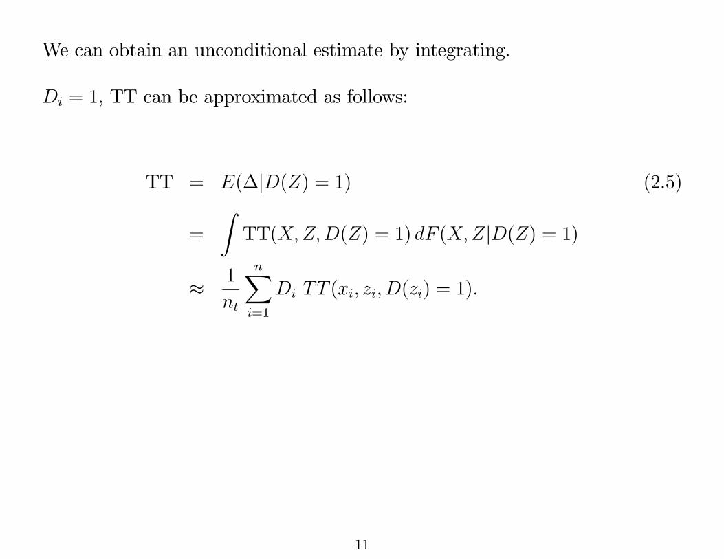
We can obtain an unconditional estimate by integrating.

= 1, TT can be approximated as follows:

TT = ( | ( ) = 1) (2.5)

=

ZTT( ( ) = 1) ( | ( ) = 1)

1 X=1

( ( ) = 1)

11

Local Average Treatment E ect (LATE) of Imbens and Angrist (1994)

LATE is defined as the expected outcome gain for those induced to receive

treatment through a change in the instrument from = to = 0 .

LATE parameter as a change in the index from = to = 0 , where

0 and and 0 are identical except for their coordinate. We could

equivalently define the treatment parameters in terms of the propensity score,

( ) = Pr( = 1| ) = 1 ( ),

denotes the cdf of the random variable .

12

The LATE parameter:

LATE( ( ) = 0 ( 0) = 1 = ) = ( | ( ) = 0 ( 0) = 1 = )

= ( 1 0) + ( 1 0 | 0 = )

= ( 1 0) + ( 1 0 | 0 )

13

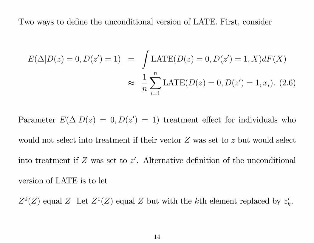
Two ways to define the unconditional version of LATE. First, consider

( | ( ) = 0 ( 0) = 1) =

ZLATE( ( ) = 0 ( 0) = 1 ) ( )

1X=1

LATE( ( ) = 0 ( 0) = 1 ) (2.6)

Parameter ( | ( ) = 0 ( 0) = 1) treatment e ect for individuals who

would not select into treatment if their vector was set to but would select

into treatment if was set to 0. Alternative definition of the unconditional

version of LATE is to let

0( ) equal Let 1( ) equal but with the th element replaced by 0 .

14

Second definition of the unconditional version of LATE,

( | ( 0( )) = 0 ( 1( )) = 1) (2.7)

=

ZLATE( ( 0( )) = 0 ( 1( )) = 1 ) ( )

1X=1

LATE( ( 0( )) = 0 ( 1( )) = 1 )

15

Marginal Treatment E ect (MTE) (Björklund and Mo tt 1987; Heckman

1997; Heckman and Smith 1998; Heckman and Vytlacil 1999, 2000a-b),

MTE( ) = ( | = = ) (2.8)

= ( 1 0) + ( 1 0 | = = )

= ( 1 0) + ( 1 0 | = )

where third equality follows ( 1 0) independent of .

16

At low values of average the outcome gain for those with unobservables

making them least likely to participate, while evaluation of the MTE parameter

at high values of is the gain for those individuals with unobservables which

make them most likely to participate. is independent of , the MTE

parameter unconditional on observed covariates can be written as

MTE( ) =

ZMTE( ) ( )

1X=1

MTE( ) = ( 1 0) + ( 1 0| = )

17

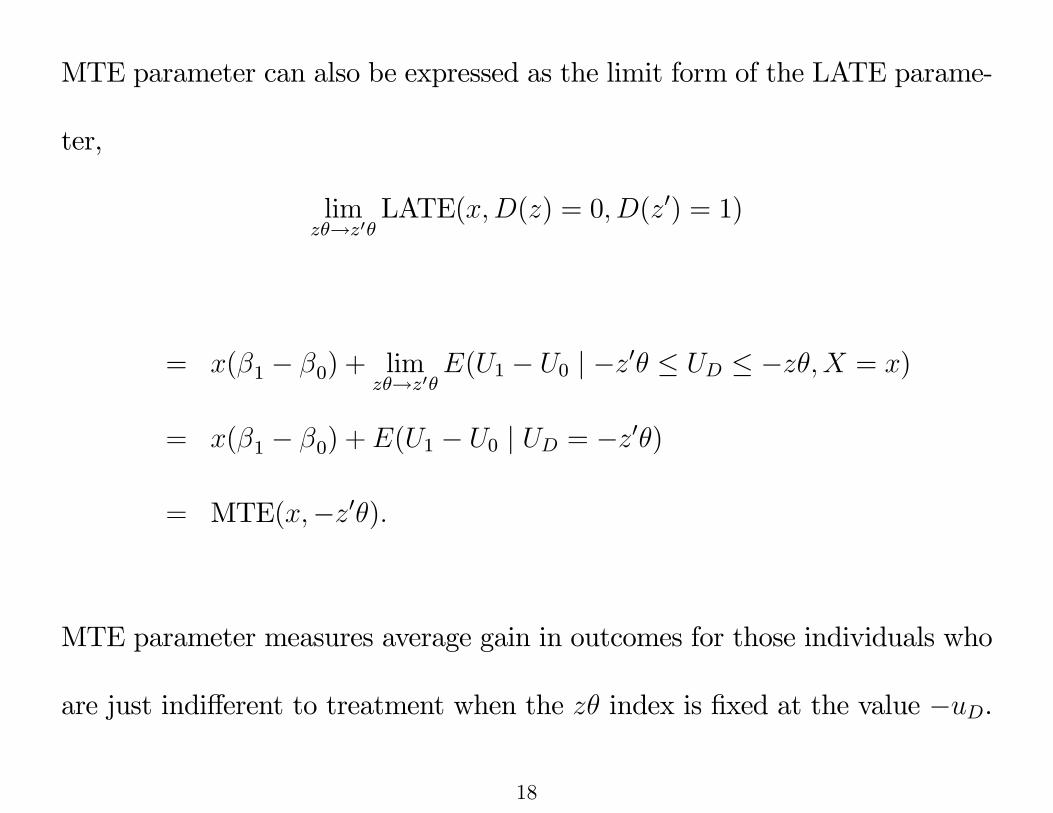
MTE parameter can also be expressed as the limit form of the LATE parame-

ter,

lim0LATE( ( ) = 0 ( 0) = 1)

= ( 1 0) + lim0

( 1 0 | 0 = )

= ( 1 0) + ( 1 0 | = 0 )

= MTE( 0 )

MTE parameter measures average gain in outcomes for those individuals who

are just indi erent to treatment when the index is fixed at the value .

18

3 Simple Expressions for the Di erent Treat-

ment Parameters in the General Case

Textbook normal model:

1

0

0

1 1 0

121 10

0 1020

19

Treatment on the Treated (TT) is:

TT( ( ) = 1) = ( 1 0) + ( 1 1 0 0)( )

( )

Thus, if Cov( 1 0 ) = 0, or 1 1 = 0 0

If Cov( 1 0 ) 0, then TT ATE

, TT ATE.

(e.g. Cramer 1946 or Johnson, Kotz, and Balakrishnan 1992)

20

( ) ( ) and , then

( | ) = +

μ( ) ( )

( ) ( )

¶

= ( ) , = ( ) . Thus,

LATE( ( ) = 0 ( 0) = 1) = ( 1 0 | 0 )) (3.1)

= ( 1 0) + ( 1 1 0 0)( 0 ) ( )

( 0 ) ( )

21

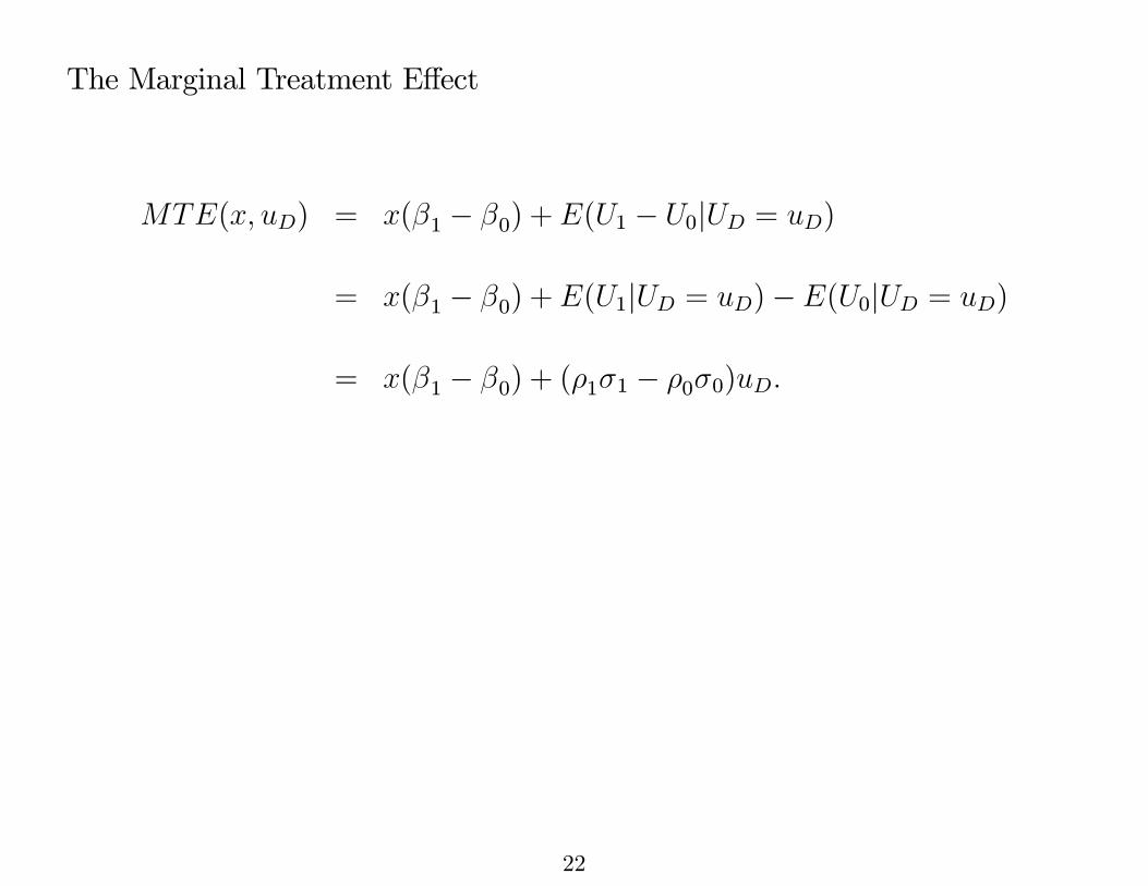
The Marginal Treatment E ect

( ) = ( 1 0) + ( 1 0| = )

= ( 1 0) + ( 1| = ) ( 0| = )

= ( 1 0) + ( 1 1 0 0)

22

Limit form of LATE.3

( ) = ( 1 0) + ( 1 1 0 0) lim( ) ( )

( ) ( )

¸

= ( 1 0) + ( 1 1 0 0) lim( ( ) ( )) ( )

( ( ) ( )) ( )

¸

= ( 1 0) + ( 1 1 0 0)

3The last line in this derivation follows from L’Hôpital’s rule.

23

Evaluating MTE when is large corresponds to case where average outcome

gain is evaluated for those individuals with unobservables making them most

likely to participate, (and conversely when is small).

When = 0, MTE = ATE as a consequence of symmetry of normal distrib-

ution.

24

Non-Normal Extensions

Following Lee (1982, 1983), trivariate Normal model can be generalized by

exploiting natural flexibility of selection equation.

In latent variable framework, selection rule assigns people to treated state

( = 1) provided 0

This is equivalent to setting = 1 when ( ) ( 0 ) for some strictly

increasing function

25

Suppose , where an absolutely continuous distribution function.

For simplicity, assume symmetry of about zero so that ( ) = 1 ( ).

˜ ( ) ( ) 1 ( ) ˜ is standard normal random variable.

26

Original model in (1) is equivalent to the transformed model:

1 =01 + 1 0 =

00 + 0 = ( 0 ) + ˜

now assume [ ˜ 1 0]0 is trivariate normal. Obtain the following selection-

corrected conditional mean functions:

( 1 | ( ) = 1 = = ) = 01 + 1 1

( ( 0 ))( 0 )

(3.2)

( 0 | ( ) = 0 = = ) = 00 0 0

( ( 0 ))1 ( 0 )

(3.3)

27

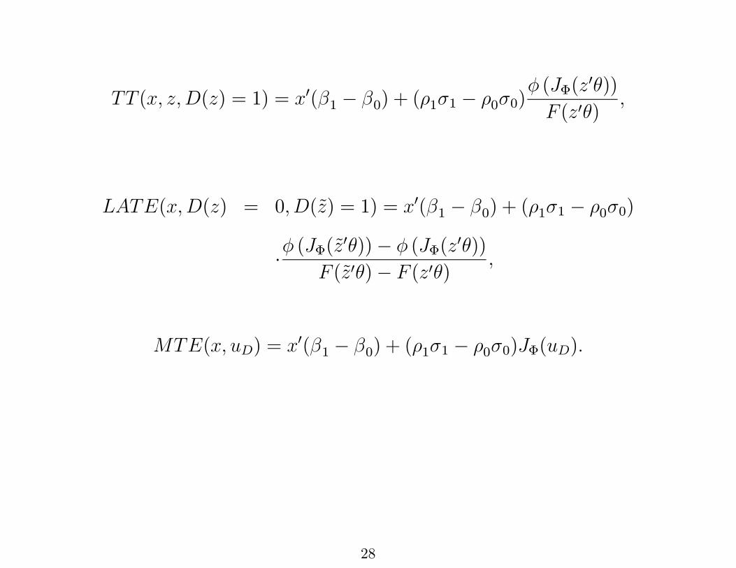
( ( ) = 1) = 0( 1 0) + ( 1 1 0 0)( ( 0 ))( 0 )

( ( ) = 0 (˜) = 1) = 0( 1 0) + ( 1 1 0 0)

· ( ( 0̃ )) ( ( 0 ))( 0̃ ) ( 0 )

( ) = 0( 1 0) + ( 1 1 0 0) ( )

28

Less straightforward generalization can be achieved by following Lee (1982,

1983) in (14) to be jointly distributed according to the Student- distribution.

( ) denotes the multivariate. Student- density function with mean ,

scale matrix (variance equal to [ ( 2)] ) and degrees of freedom.4

Let denote the standardized univariate Student density with mean 0 and

scale parameter equal to 1. Let denote the associated cdf.

4The mean exists when 1 and the variance exists when 2

29

Letting , we define ( ) 1( ( )) as before, again noting that

( ) = ( ) Assume [ ˜ 1 0]0 has a trivariate (0 ) density.

( 1 | ( ) = 1 = = ) = 01

+ 1 1

μ+ [ ( 0 )]2

1

¶μ( ( 0 ))( 0 )

¶¸

( 0 | ( ) = 0 = = ) = 00

0 0

μ+ [ ( 0 )]2

1

¶μ( ( 0 ))1 ( 0 )

¶¸

30

( )

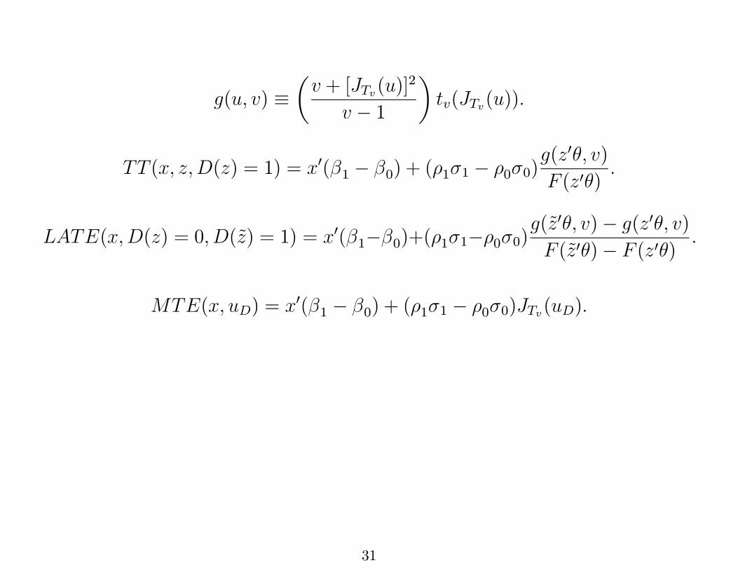
μ+ [ ( )]2

1

¶( ( ))

( ( ) = 1) = 0( 1 0) + ( 1 1 0 0)( 0 )

( 0 )

( ( ) = 0 (˜) = 1) = 0( 1 0)+( 1 1 0 0)( 0̃ ) ( 0 )

( 0̃ ) ( 0 )

( ) = 0( 1 0) + ( 1 1 0 0) ( )

31

3.1 Estimation

1. Obtain ˆ from a probit model on the decision to take the treatment.

2. Compute the appropriate selection correction terms evaluated at ˆ,

(i.e. ( ˆ) ( ˆ) when = 1,

and ( ˆ) (1 ( ˆ)) when = 0 )

32

3. Run treatment-outcome-specific regressions (for the groups { : =

1} and { : = 0}) with the inclusion of the appropriate selection-

correction terms obtained from the previous step.

4. Given ˆ0 ˆ1 1̂ 1 and 0̂ 0 obtained from step 3, and ˆ from step (1),

use these parameter estimates to obtain point estimates of the treatment

parameters for given , , and 0. Alternatively, one could integrate

over the distribution of the characteristics to obtain unconditional esti-

mates, as suggested in section 2.

33

Table 1Point Estimates and Standard Errors of Alternate Treatment Parameters

Outcome Errors / Link Function ATE TT LATE

Normal/Normal .092 .039 .079(SSR=345.25) (.03) (.04) (.03)

tv=2 / Logit .061 .036 .053(SSR = 346.09) (.02) (.03) (.02)

tv=3 / Logit .073 .035 .062(SSR = 345.79) (.02) (.03) (.02)

tv=4 / Logit .079 .035 .067(SSR = 345.61) (.02) (.04) (.03)

tv=5 / Logit .082 .034 .069(SSR = 345.51) (.03) (.04) (.03)

tv=6 / Logit .084 .034 .071(SSR = 345.44) (.03) (.04) (.03)

tv=8 / Logit .085 .034 .073(SSR = 345.36) (.03) (.04) (.03)

tv=12 / Logit .087 .034 .073(SSR = 345.29) (.03) (.04) (.04)

tv=24 / Logit .088 .033 .075(SSR = 345.23) (.04) (.04) (.03)

tv=2 / tv=2 .067 .028 .058(SSR = 345.68) (.03) (.04) (.03)

tv=3 / tv=3 .075 .030 .063(SSR = 345.56) (.03) (.04) (.03)

tv=4 / tv=4 .079 .031 .066(SSR = 345.48) (.03) (.04) (.03)

tv=5 / tv=5 .082 .032 .069(SSR = 345.43) (.03) (.04) (.03)

tv=6 / tv=6 .084 .033 .070(SSR = 345.40) (.03) (.04) (.03)

tv=8 / tv=8 .086 .034 .072(SSR = 345.36) (.03) (.04) (.03)

tv=12 / tv=12 .088 .036 .075(SSR = 345.32) (.03) (.04) (.03)

tv=24 / tv=24 .090 .037 .077(SSR = 345.29) (.03) (.04) (.03)

34

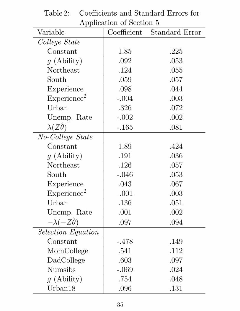
Table 2: Coe cients and Standard Errors forApplication of Section 5

Variable Coe cient Standard Error

College StateConstant 1.85 .225g (Ability) .092 .053Northeast .124 .055South .059 .057Experience .098 .044Experience2 -.004 .003Urban .326 .072Unemp. Rate -.002 .002

(Zˆ) -.165 .081

No-College StateConstant 1.89 .424g (Ability) .191 .036Northeast .126 .057South -.046 .053Experience .043 .067Experience2 -.001 .003Urban .136 .051Unemp. Rate .001 .002

( Zˆ) .097 .094

Selection EquationConstant -.478 .149MomCollege .541 .112DadCollege .603 .097Numsibs -.069 .024g (Ability) .754 .048Urban18 .096 .131

35

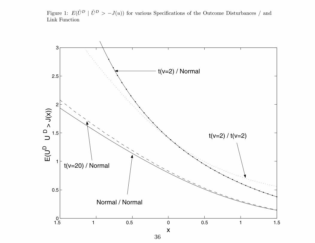
Figure 1: E( ~UD j ~UD > ¡J(u)) for various Speci¯cations of the Outcome Disturbances / andLink Function

1.5 1 0.5 0 0.5 1 1.50

0.5

1

1.5

2

2.5

3E

(UD

UD

> J

(x))

x

Normal / Normal

t(v=2) / Normal

t(v=2) / t(v=2)

t(v=20) / Normal

36

Distributions of Treatment on the Treated and Marginal Treatment E®ects UsingNormal and t2 Models. Generated NORMAL Data. 1,000 Replications with N = 1,500.

Figure 2: Treatment on the Treated with Z = ¡2: True Value ¼ 2:28

1.4 1.6 1.8 2 2.2 2.4 2.6 2.8 3 3.20

0.2

0.4

0.6

0.8

1

1.2

1.4

1.6

1.8

2

Normalt(2)

37

Figure 3: Marginal Treatment E®ect with uD = 1: True Value ¼ 1:54

1.4 1.6 1.8 2 2.2 2.4 2.6 2.80

0.5

1

1.5

2

2.5

3

Marginal Treatment Effect Z=2. True MTE 2.08.

t(4)

Normal

38

Distributions of Treatment on the Treated and Marginal Treatment E®ects UsingNormal and t2 Models. Generated t4 Data. 1,000 Replications with N = 2,500.

Figure 4: Treatment on the Treated with Z = ¡2: True Value ¼ 2:64

1.8 2 2.2 2.4 2.6 2.8 3 3.2 3.4 3.60

0.2

0.4

0.6

0.8

1

1.2

1.4

1.6

1.8

2

Treatment on the Treated Z=2. True TT 2.64.

t(4)Normal

39

Figure 5: Marginal Treatment E®ect with uD = 2: True Value ¼ 2:08

1.4 1.6 1.8 2 2.2 2.4 2.6 2.80

0.5

1

1.5

2

2.5

3

Marginal Treatment Effect Z=2. True MTE 2.08.

t(4)

Normal

40

Figure 6: Probability of Correctly Choosing Normal Model Over t2 Model Using MSE Criterion.1,000 Iterations

33

0 100 200 300 400 500 600 700 800 900 10000.5

0.55

0.6

0.65

0.7

0.75

0.8

0.85

0.9

Number of Observations

Pro

babi

lity

of C

hoos

ing

Cor

rect

ly

Probability of Selecting Correct Model Using MSE Criterion. 1,000 Iterations

ρ1D = .95, ρ0D = .1

ρ1D = .5, ρ0D = .1

ρ1D = .2, ρ0D = .1

41

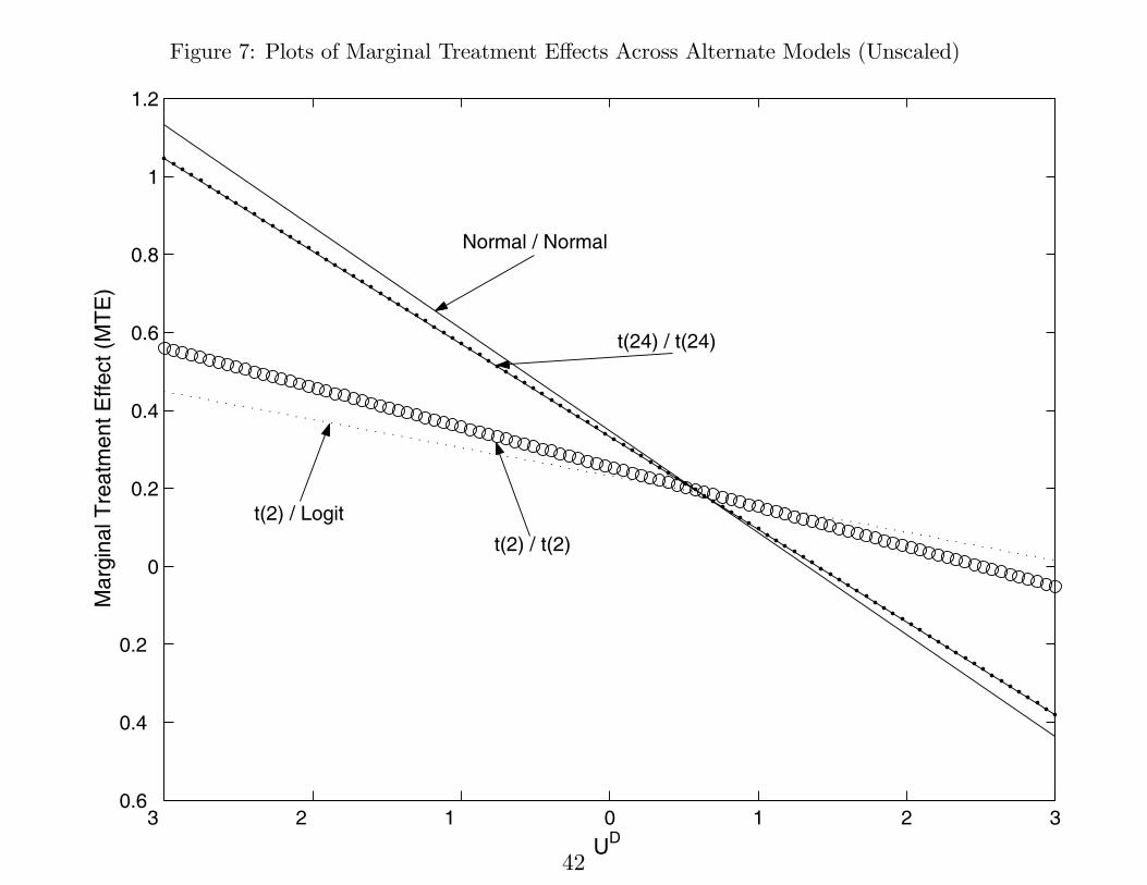
Figure 7: Plots of Marginal Treatment E®ects Across Alternate Models (Unscaled)

3 2 1 0 1 2 30.6

0.4

0.2

0

0.2

0.4

0.6

0.8

1

1.2

UD

Mar

gina

l Tre

atm

ent E

ffect

(M

TE

)

Normal / Normal

t(24) / t(24)

t(2) / Logit

t(2) / t(2)

42