foundations of engineering economy edition chapter 1.pdf1 chapter 1 foundations of engineering...

1

1C h a p t e r

Foundations ofEngineering Economy

T he need for engineering economy is primarily motivated by the work thatengineers do in performing analysis, synthesizing, and coming to a conclu-sion as they work on projects of all sizes. In other words, engineering econ-

omy is at the heart of making decisions. These decisions involve the fundamentalelements of cash flows of money, time, and interest rates. This chapter introducesthe basic concepts and terminology necessary for an engineer to combine thesethree essential elements in organized, mathematically correct ways to solve prob-lems that will lead to better decisions.

Royalty-Free/CORBIS

bLa01293_ch01_001-026 8/4/07 7:03 PM

2

Purpose: Understand the fundamental concepts of engineering economy.

Doubling time

Spreadsheet functions

Cash flows

Symbols

Simple and compound interest

Equivalence

Interest rate

Study approach and terms

Definition and role

Objectives

1. Determine the role of engineering economy in thedecision-making process.

2. Identify what is needed to successfully perform anengineering economy study.

3. Perform calculations about interest rate and rate of return.

4. Understand what equivalence means in economic terms.

5. Calculate simple interest and compound interest for oneor more interest periods.

6. Identify and use engineering economy terminology andsymbols.

7. Understand cash flows, their estimation, and how tographically represent them.

8. Use the rule of 72 to estimate a compound interest rate ornumber of years for an amount of money to double in size.

9. Formulate Excel© functions used in engineering economy.

bLa01293_ch01_001-026 8/7/07 5:22 PM

1.2 Performing an Engineering Economy Study 3

1.1 WHAT IS ENGINEERING ECONOMY?

Before we begin to develop the fundamental concepts upon which engineeringeconomy is based, it would be appropriate to define what is meant by engineeringeconomy. In the simplest of terms, engineering economy is a collection of tech-niques that simplify comparisons of alternatives on an economic basis. In definingwhat engineering economy is, it might also be helpful to define what it is not. Engi-neering economy is not a method or process for determining what the alternativesare. On the contrary, engineering economy begins only after the alternatives havebeen identified. If the best alternative is actually one that the engineer has not evenrecognized as an alternative, then all of the engineering economic analysis tools inthis book will not result in its selection.

While economics will be the sole criterion for selecting the best alternatives inthis book, real-world decisions usually include many other factors in the decision-making process. For example, in determining whether to build a nuclear-powered,gas-fired, or coal-fired power plant, factors such as safety, air pollution, public accept-ance, water demand, waste disposal, global warming, and many others would beconsidered in identifying the best alternative. The inclusion of other factors (besideseconomics) in the decision-marking process is called multiple attribute analysis. Thistopic is introduced in Appendix C.

1.2 PERFORMING AN ENGINEERING ECONOMY STUDY

In order to apply economic analysis techniques, it is necessary to understand thebasic terminology and fundamental concepts that form the foundation for engineering-economy studies. Some of these terms and concepts are described below.

1.2.1 AlternativesAn alternative is a stand-alone solution for a given situation. We are faced with alter-natives in virtually everything we do, from selecting the method of transportation weuse to get to work every day to deciding between buying a house or renting one.Similarly, in engineering practice, there are always several ways of accomplishing agiven task, and it is necessary to be able to compare them in a rational manner sothat the most economical alternative can be selected. The alternatives in engineeringconsiderations usually involve such items as purchase cost (first cost), anticipateduseful life, yearly costs of maintaining assets (annual maintenance and operatingcosts), anticipated resale value (salvage value), and the interest rate. After the factsand all the relevant estimates have been collected, an engineering economy analysiscan be conducted to determine which is best from an economic point of view.

1.2.2 Cash FlowsThe estimated inflows (revenues) and outflows (costs) of money are called cashflows. These estimates are truly the heart of an engineering economic analysis.

bLa01293_ch01_001-026 8/7/07 5:22 PM

4 Chapter 1 Foundations of Engineering Economy

They also represent the weakest part of the analysis, because most of the numbersare judgments about what is going to happen in the future. After all, who can accu-rately predict the price of oil next week, much less next month, next year, or nextdecade? Thus, no matter how sophisticated the analysis technique, the end resultis only as reliable as the data that it is based on.

1.2.3 Alternative SelectionEvery situation has at least two alternatives. In addition to the one or more formu-lated alternatives, there is always the alternative of inaction, called the do-nothing(DN) alternative. This is the as-is or status quo condition. In any situation, whenone consciously or subconsciously does not take any action, he or she is actuallyselecting the DN alternative. Of course, if the status quo alternative is selected, thedecision-making process should indicate that doing nothing is the most favorableeconomic outcome at the time the evaluation is made. The procedures developedin this book will enable you to consciously identify the alternative(s) that is (are)economically the best.

1.2.4 Evaluation CriteriaWhether we are aware of it or not, we use criteria every day to choose betweenalternatives. For example, when you drive to campus, you decide to take the “best”route. But how did you define best? Was the best route the safest, shortest, fastest,cheapest, most scenic, or what? Obviously, depending upon which criterion or com-bination of criteria is used to identify the best, a different route might be selectedeach time. In economic analysis, financial units (dollars or other currency) are gen-erally used as the tangible basis for evaluation. Thus, when there are several waysof accomplishing a stated objective, the alternative with the lowest overall cost orhighest overall net income is selected.

1.2.5 Intangible FactorsIn many cases, alternatives have noneconomic or intangible factors that are diffi-cult to quantify. When the alternatives under consideration are hard to distinguisheconomically, intangible factors may tilt the decision in the direction of one of thealternatives. A few examples of noneconomic factors are goodwill, convenience,friendship, and morale.

1.2.6 Time Value of MoneyIt is often said that money makes money. The statement is indeed true, for ifwe elect to invest money today, we inherently expect to have more money inthe future. If a person or company borrows money today, by tomorrow more thanthe original loan principal will be owed. This fact is also explained by the timevalue of money.

bLa01293_ch01_001-026 8/4/07 7:03 PM

1.3 Interest Rate, Rate of Return, and MARR 5

The change in the amount of money over a given time period is called the

time value of money; it is the most important concept in engineering

economy.

The time value of money can be taken into account by several methods in aneconomy study, as we will learn. The method’s final output is a measure of worth,for example, rate of return. This measure is used to accept/reject an alternative.

1.3 INTEREST RATE, RATE OF RETURN, AND MARR

Interest is the manifestation of the time value of money, and it essentially rep-resents “rent” paid for use of the money. Computationally, interest is the differ-ence between an ending amount of money and the beginning amount. If thedifference is zero or negative, there is no interest. There are always two perspectivesto an amount of interest—interest paid and interest earned. Interest is paid whena person or organization borrows money (obtains a loan) and repays a largeramount. Interest is earned when a person or organization saves, invests, or lendsmoney and obtains a return of a larger amount. The computations and numeri-cal values are essentially the same for both perspectives, but they are interpreteddifferently.

Interest paid or earned is determined by using the relation

[1.1]

When interest over a specific time unit is expressed as a percentage of the origi-nal amount (principal), the result is called the interest rate or rate of return (ROR).

[1.2]

The time unit of the interest rate is called the interest period. By far the most com-mon interest period used to state an interest rate is 1 year. Shorter time periods canbe used, such as, 1% per month. Thus, the interest period of the interest rate shouldalways be included. If only the rate is stated, for example, 8.5%, a 1-year interestperiod is assumed.

The term return on investment (ROI) is used equivalently with ROR in differ-ent industries and settings, especially where large capital funds are committed toengineering-oriented programs. The term interest rate paid is more appropriate forthe borrower’s perspective, while rate of return earned is better from the investor’sperspective.

Interest rate or rate of return �interest accrued per time unit

original amount� 100%

Interest � end amount � original amount

EXAMPLE 1.1An employee at LaserKinetics.com borrows $10,000 on May 1 and must repaya total of $10,700 exactly 1 year later. Determine the interest amount and theinterest rate paid.

bLa01293_ch01_001-026 8/4/07 7:03 PM


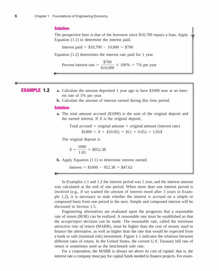
In Examples 1.1 and 1.2 the interest period was 1 year, and the interest amountwas calculated at the end of one period. When more than one interest period isinvolved (e.g., if we wanted the amount of interest owed after 3 years in Exam-ple 1.2), it is necessary to state whether the interest is accrued on a simple orcompound basis from one period to the next. Simple and compound interest will bediscussed in Section 1.5.

Engineering alternatives are evaluated upon the prognosis that a reasonablerate of return (ROR) can be realized. A reasonable rate must be established so thatthe accept/reject decision can be made. The reasonable rate, called the minimumattractive rate of return (MARR), must be higher than the cost of money used tofinance the alternative, as well as higher than the rate that would be expected froma bank or safe (minimal risk) investment. Figure 1-1 indicates the relations betweendifferent rates of return. In the United States, the current U.S. Treasury bill rate ofreturn is sometimes used as the benchmark safe rate.

For a corporation, the MARR is always set above its cost of capital, that is, theinterest rate a company must pay for capital funds needed to finance projects. For exam-

SolutionThe perspective here is that of the borrower since $10,700 repays a loan. ApplyEquation [1.1] to determine the interest paid.

Equation [1.2] determines the interest rate paid for 1 year.

Percent interest rate �$700

$10,000� 100% � 7% per year

Interest paid � $10,700 � 10,000 � $700

EXAMPLE 1.2 a. Calculate the amount deposited 1 year ago to have $1000 now at an inter-est rate of 5% per year.

b. Calculate the amount of interest earned during this time period.

Solutiona. The total amount accrued ($1000) is the sum of the original deposit and

the earned interest. If X is the original deposit,

The original deposit is

b. Apply Equation [1.1] to determine interest earned.

Interest � $1000 � 952.38 � $47.62

X �1000

1.05� $952.38

$1000 � X � X(0.05) � X(1 � 0.05) � 1.05X Total accrued � original amount � original amount (interest rate)

bLa01293_ch01_001-026 9/7/07 10:59 PM

1.3 Interest Rate, Rate of Return, and MARR 7

ple, if a corporation can borrow capital funds at an average of 5% per year and expectsto clear at least 6% per year on a project, the minimum MARR will be 11% per year.

The MARR is also referred to as the hurdle rate; that is, a financially viableproject’s expected ROR must meet or exceed the hurdle rate. Note that the MARRis not a rate calculated like the ROR; MARR is established by financial managersand is used as a criterion for accept/reject decisions. The following inequality mustbe correct for any accepted project.

Descriptions and problems in the following chapters use stated MARR values withthe assumption that they are set correctly relative to the cost of capital and theexpected rate of return. If more understanding of capital funds and the establish-ment of the MARR is required, refer to Section 13.5 for further detail.

An additional economic consideration for any engineering economy study isinflation. In simple terms, bank interest rates reflect two things: a so-called realrate of return plus the expected inflation rate. The safest investments (such as U.S.government bonds) typically have a 3% to 4% real rate of return built into theiroverall interest rates. Thus, an interest rate of, say, 9% per year on a U.S. govern-ment bond means that investors expect the inflation rate to be in the range of 5%to 6% per year. Clearly, then, inflation causes interest rates to rise. Inflation is dis-cussed in detail in Chapter 10.

ROR � MARR � cost of capital

Rate of return,percent

Expected rate of return ona new project

Rate of return on“safe investment”

Range for the rate of return onpending projects

MARRAll proposals must offerat least MARR tobe considered

Range of cost of capital

FIGURE 1.1MARR relative to costof capital and otherrate of return values.

bLa01293_ch01_001-026 8/4/07 7:03 PM


1.4 EQUIVALENCE

Equivalent terms are used often in the transfer between scales and units. For exam-ple, 1000 meters is equal to (or equivalent to) 1 kilometer, 12 inches equals 1 foot,and 1 quart equals 2 pints or 0.946 liter.

In engineering economy, when considered together, the time value of moneyand the interest rate help develop the concept of economic equivalence, whichmeans that different sums of money at different times would be equal in economicvalue. For example, if the interest rate is 6% per year, $100 today (present time)is equivalent to $106 one year from today.

So, if someone offered you a gift of $100 today or $106 one year from today, itwould make no difference which offer you accepted from an economic perspec-tive. In either case you have $106 one year from today. However, the two sumsof money are equivalent to each other only when the interest rate is 6% per year.At a higher or lower interest rate, $100 today is not equivalent to $106 one yearfrom today.

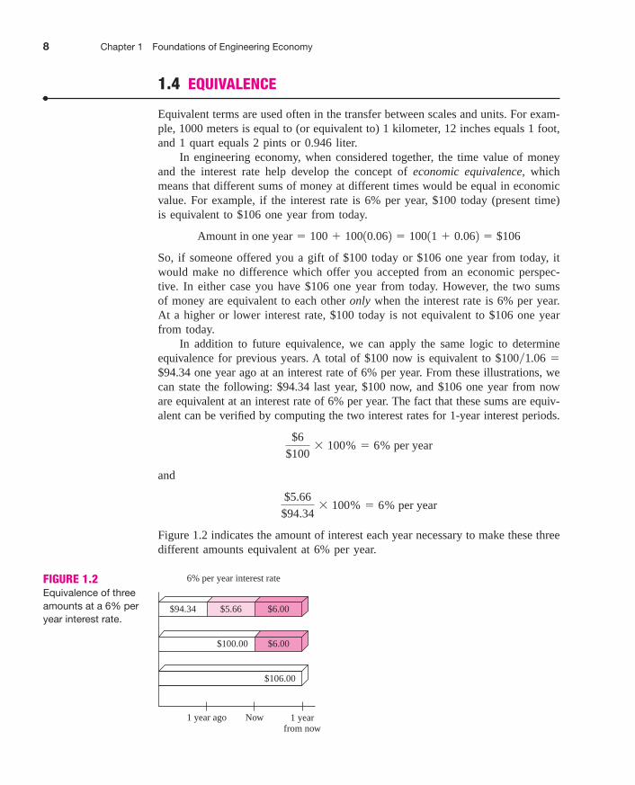
In addition to future equivalence, we can apply the same logic to determineequivalence for previous years. A total of $100 now is equivalent to $100�1.06 �$94.34 one year ago at an interest rate of 6% per year. From these illustrations, wecan state the following: $94.34 last year, $100 now, and $106 one year from noware equivalent at an interest rate of 6% per year. The fact that these sums are equiv-alent can be verified by computing the two interest rates for 1-year interest periods.

and

Figure 1.2 indicates the amount of interest each year necessary to make these threedifferent amounts equivalent at 6% per year.

$5.66

$94.34� 100% � 6% per year

$6

$100� 100% � 6% per year

Amount in one year � 100 � 10010.062 � 10011 � 0.062 � $106

FIGURE 1.2Equivalence of threeamounts at a 6% peryear interest rate.

1 year ago

6% per year interest rate

Now

$100.00 $6.00

$106.00

1 yearfrom now

$94.34 $5.66 $6.00

bLa01293_ch01_001-026 8/4/07 7:03 PM

1.5 Simple and Compound Interest 9

1.5 SIMPLE AND COMPOUND INTEREST

The terms interest, interest period, and interest rate were introduced in Section 1.3for calculating equivalent sums of money for one interest period in the past andone period in the future. However, for more than one interest period, the terms sim-ple interest and compound interest become important.

Simple interest is calculated using the principal only, ignoring any interestaccrued in preceding interest periods. The total simple interest over several peri-ods is computed as

[1.3]

where the interest rate is expressed in decimal form.

Interest � (principal)(number of periods)(interest rate)

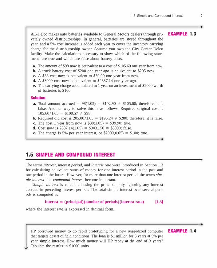
EXAMPLE 1.4HP borrowed money to do rapid prototyping for a new ruggedized computerthat targets desert oilfield conditions. The loan is $1 million for 3 years at 5% peryear simple interest. How much money will HP repay at the end of 3 years?Tabulate the results in $1000 units.

AC-Delco makes auto batteries available to General Motors dealers through pri-vately owned distributorships. In general, batteries are stored throughout theyear, and a 5% cost increase is added each year to cover the inventory carryingcharge for the distributorship owner. Assume you own the City Center Delcofacility. Make the calculations necessary to show which of the following state-ments are true and which are false about battery costs.

a. The amount of $98 now is equivalent to a cost of $105.60 one year from now.b. A truck battery cost of $200 one year ago is equivalent to $205 now.c. A $38 cost now is equivalent to $39.90 one year from now.d. A $3000 cost now is equivalent to $2887.14 one year ago.e. The carrying charge accumulated in 1 year on an investment of $2000 worth

of batteries is $100.

Solutiona. Total amount accrued � 98(1.05) � $102.90 � $105.60; therefore, it is

false. Another way to solve this is as follows: Required original cost is105.60�1.05 � $100.57 � $98.

b. Required old cost is 205.00�1.05 � $195.24 � $200; therefore, it is false.c. The cost 1 year from now is $38(1.05) � $39.90; true.d. Cost now is 2887.14(1.05) � $3031.50 � $3000; false.e. The charge is 5% per year interest, or $2000(0.05) � $100; true.

EXAMPLE 1.3

bLa01293_ch01_001-026 8/4/07 7:03 PM


For compound interest, the interest accrued for each interest period is calculatedon the principal plus the total amount of interest accumulated in all previous periods.Thus, compound interest means interest on top of interest. Compound interestreflects the effect of the time value of money on the interest also. Now the interestfor one period is calculated as

[1.4]Interest � (principal � all accrued interest)(interest rate)

EXAMPLE 1.5 If HP borrows $1,000,000 from a different source at 5% per year compoundinterest, compute the total amount due after 3 years. Compare the results of thisand the previous example.

SolutionThe interest for each of the 3 years in $1000 units is

Total interest for 3 years from Equation [1.3] is

The amount due after 3 years in $1000 units is

The $50,000 interest accrued in the first year and the $50,000 accrued inthe second year do not earn interest. The interest due each year is calculatedonly on the $1,000,000 principal.

The details of this loan repayment are tabulated in Table 1.1 from the per-spective of the borrower. The year zero represents the present, that is, when themoney is borrowed. No payment is made until the end of year 3. The amountowed each year increases uniformly by $50,000, since simple interest is figuredon only the loan principal.

Total due � $1000 � 150 � $1150

Total interest � 1000132 10.052 � $150

Interest per year � 100010.052 � $50

TABLE 1.1 Simple Interest Computations (in $1000 units)

(1) (2) (3) (4) (5)

End of Amount Amount Amount

Year Borrowed Interest Owed Paid

0 $1000

1 — $50 $1050 $ 0

2 — 50 1100 0

3 — 50 1150 1150

bLa01293_ch01_001-026 8/4/07 7:03 PM


Another and shorter way to calculate the total amount due after 3 years inExample 1.5 is to combine calculations rather than perform them on a year-by-year basis. The total due each year is as follows:

Year 1:Year 2:Year 3:

The year 3 total is calculated directly; it does not require the year 2 total. In gen-eral formula form,

This fundamental relation is used many times in upcoming chapters.

Total due after a number of years � principal(1 � interest rate)number of years

$1000(1.05)3 � $1157.63$1000(1.05)2 � $1102.50$1000(1.05)1 � $1050.00

TABLE 1.2 Compound Interest Computations (in $1000 units),Example 1.5

(1) (2) (3) (4) (5)

End of Amount Amount Amount

Year Borrowed Interest Owed Paid

0 $1000

1 — $50.00 $1050.00 $ 0

2 — 52.50 1102.50 0

3 — 55.13 1157.63 1157.63

SolutionThe interest and total amount due each year are computed separately usingEquation [1.4]. In $1000 units,

Year 1 interest:

Total amount due after year 1:

Year 2 interest:


Year 3 interest:


The details are shown in Table 1.2. The repayment plan is the same as that forthe simple interest example—no payment until the principal plus accrued inter-est is due at the end of year 3. An extra ofinterest is paid compared to simple interest over the 3-year period.

Comment: The difference between simple and compound interest grows signif-icantly each year. If the computations are continued for more years, for exam-ple, 10 years, the difference is $128,894; after 20 years compound interest is$653,298 more than simple interest.

$1,157,630 � 1,150,000 � $7,630

$1102.50 � 55.13 � $1157.63

$1102.5010.052 � $55.13

$1050 � 52.50 � $1102.50

$105010.052 � $52.50

$1000 � 50.00 � $1050.00

$100010.052 � $50.00

bLa01293_ch01_001-026 8/7/07 5:22 PM


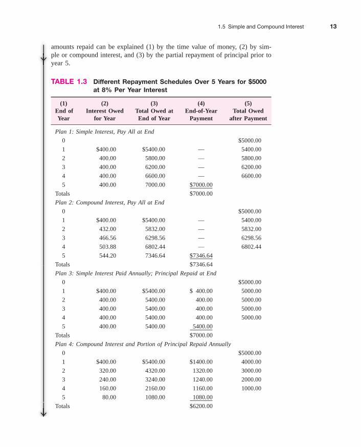
We combine the concepts of interest rate, simple interest, compound interest, andequivalence to demonstrate that different loan repayment plans may be equivalent, butthey may differ substantially in monetary amounts from one year to another. This alsoshows that there are many ways to take into account the time value of money. Thefollowing example illustrates equivalence for five different loan repayment plans.

EXAMPLE 1.6 a. Demonstrate the concept of equivalence using the different loan repaymentplans described below. Each plan repays a $5000 loan in 5 years at 8%interest per year.� Plan 1: Simple interest, pay all at end. No interest or principal is paid

until the end of year 5. Interest accumulates each year on the principalonly.

� Plan 2: Compound interest, pay all at end. No interest or principal ispaid until the end of year 5. Interest accumulates each year on the totalof principal and all accrued interest.

� Plan 3: Simple interest paid annually, principal repaid at end. Theaccrued interest is paid each year, and the entire principal is repaid atthe end of year 5.

� Plan 4: Compound interest and portion of principal repaid annually.

The accrued interest and one-fifth of the principal (or $1000) is repaideach year. The outstanding loan balance decreases each year, so the inter-est for each year decreases.

� Plan 5: Equal payments of compound interest and principal made

annually. Equal payments are made each year with a portion goingtoward principal repayment and the remainder covering the accrued inter-est. Since the loan balance decreases at a rate slower than that in plan4 due to the equal end-of-year payments, the interest decreases, but at aslower rate.

b. Make a statement about the equivalence of each plan at 8% simple or com-pound interest, as appropriate.

Solutiona. Table 1.3 presents the interest, payment amount, total owed at the end of

each year, and total amount paid over the 5-year period (column 4 totals).The amounts of interest (column 2) are determined as follows:

Plan 1

Plan 2

Plan 3

Plan 4

Plan 5

Note that the amounts of the annual payments are different for each repaymentschedule and that the total amounts repaid for most plans are different, eventhough each repayment plan requires exactly 5 years. The difference in the total

Compound interest � (total owed previous year)(0.08)Compound interest � (total owed previous year)(0.08)Simple interest � (original principal)(0.08)Compound interest � (total owed previous year)(0.08)Simple interest � (original principal)(0.08)

bLa01293_ch01_001-026 8/4/07 7:03 PM


amounts repaid can be explained (1) by the time value of money, (2) by sim-ple or compound interest, and (3) by the partial repayment of principal prior toyear 5.

TABLE 1.3 Different Repayment Schedules Over 5 Years for $5000at 8% Per Year Interest

(1) (2) (3) (4) (5)

End of Interest Owed Total Owed at End-of-Year Total Owed

Year for Year End of Year Payment after Payment

Plan 1: Simple Interest, Pay All at End0 $5000.00

1 $400.00 $5400.00 — 5400.00

2 400.00 5800.00 — 5800.00

3 400.00 6200.00 — 6200.00

4 400.00 6600.00 — 6600.00

5 400.00 7000.00 $7000.00

Totals $7000.00

Plan 2: Compound Interest, Pay All at End0 $5000.00

1 $400.00 $5400.00 — 5400.00

2 432.00 5832.00 — 5832.00

3 466.56 6298.56 — 6298.56

4 503.88 6802.44 — 6802.44

5 544.20 7346.64 $7346.64

Totals $7346.64

Plan 3: Simple Interest Paid Annually; Principal Repaid at End0 $5000.00

1 $400.00 $5400.00 $ 400.00 5000.00

2 400.00 5400.00 400.00 5000.00

3 400.00 5400.00 400.00 5000.00

4 400.00 5400.00 400.00 5000.00

5 400.00 5400.00 5400.00

Totals $7000.00

Plan 4: Compound Interest and Portion of Principal Repaid Annually0 $5000.00

1 $400.00 $5400.00 $1400.00 4000.00

2 320.00 4320.00 1320.00 3000.00

3 240.00 3240.00 1240.00 2000.00

4 160.00 2160.00 1160.00 1000.00

5 80.00 1080.00 1080.00

Totals $6200.00

bLa01293_ch01_001-026 8/4/07 7:03 PM


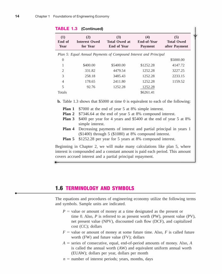
TABLE 1.3 (Continued)

(1) (2) (3) (4) (5)

End of Interest Owed Total Owed at End-of-Year Total Owed

Year for Year End of Year Payment after Payment

1.6 TERMINOLOGY AND SYMBOLS

The equations and procedures of engineering economy utilize the following termsand symbols. Sample units are indicated.

value or amount of money at a time designated as the present ortime 0. Also, P is referred to as present worth (PW), present value (PV),net present value (NPV), discounted cash flow (DCF), and capitalizedcost (CC); dollars

value or amount of money at some future time. Also, F is called futureworth (FW) and future value (FV); dollars

series of consecutive, equal, end-of-period amounts of money. Also, Ais called the annual worth (AW) and equivalent uniform annual worth(EUAW); dollars per year, dollars per month

number of interest periods; years, months, days n �

A �

F �

P �

Plan 5: Equal Annual Payments of Compound Interest and Principal0 $5000.00

1 $400.00 $5400.00 $1252.28 4147.72

2 331.82 4479.54 1252.28 3227.25

3 258.18 3485.43 1252.28 2233.15

4 178.65 2411.80 1252.28 1159.52

5 92.76 1252.28 1252.28

Totals $6261.41

b. Table 1.3 shows that $5000 at time 0 is equivalent to each of the following:

Plan 1 $7000 at the end of year 5 at 8% simple interest.Plan 2 $7346.64 at the end of year 5 at 8% compound interest.Plan 3 $400 per year for 4 years and $5400 at the end of year 5 at 8%

simple interest.Plan 4 Decreasing payments of interest and partial principal in years 1

($1400) through 5 ($1080) at 8% compound interest.Plan 5 $1252.28 per year for 5 years at 8% compound interest.

Beginning in Chapter 2, we will make many calculations like plan 5, whereinterest is compounded and a constant amount is paid each period. This amountcovers accrued interest and a partial principal repayment.

bLa01293_ch01_001-026 9/4/07 12:21 PM

1.6 Terminology and Symbols 15

interest rate or rate of return per time period; percent per year, percentper month, percent per day

time, stated in periods; years, months, days

The symbols P and F represent one-time occurrences: A occurs with the same valueeach interest period for a specified number of periods. It should be clear that apresent value P represents a single sum of money at some time prior to a futurevalue F or prior to the first occurrence of an equivalent series amount A.

It is important to note that the symbol A always represents a uniform amount(i.e., the same amount each period) that extends through consecutive interest peri-ods. Both conditions must exist before the series can be represented by A.

The interest rate i is assumed to be a compound rate, unless specifically statedas simple interest. The rate i is expressed in percent per interest period, for exam-ple, 12% per year. Unless stated otherwise, assume that the rate applies through-out the entire n years or interest periods. The decimal equivalent for i is alwaysused in engineering economy computations.

All engineering economy problems involve the element of time n and interestrate i. In general, every problem will involve at least four of the symbols P, F, A,n, and i, with at least three of them estimated or known.

t �

i �

In Examples 1.7 and 1.8, the P value is a receipt to the borrower, and F or Ais a disbursement from the borrower. It is equally correct to use these symbols inthe reverse roles.

EXAMPLE 1.7A new college graduate has a job with Boeing Aerospace. She plans to borrow$10,000 now to help in buying a car. She has arranged to repay the entire prin-cipal plus 8% per year interest after 5 years. Identify the engineering economysymbols involved and their values for the total owed after 5 years.

SolutionIn this case, P and F are involved, since all amounts are single payments, as wellas n and i. Time is expressed in years.

The future amount F is unknown.

F � ?n � 5 yearsi � 8% per yearP � $10,000

EXAMPLE 1.8Assume you borrow $2000 now at 7% per year for 10 years and must repay theloan in equal yearly payments. Determine the symbols involved and their values.

SolutionTime is in years.

n � 10 years

i � 7% per year

A � ? per year for 5 years

P � $2000

bLa01293_ch01_001-026 9/4/07 12:21 PM


EXAMPLE 1.10

1.7 CASH FLOWS: THEIR ESTIMATION AND DIAGRAMMING

Cash flows are inflows and outflows of money. These cash flows may be estimatesor observed values. Every person or company has cash receipts—revenue andincome (inflows); and cash disbursements—expenses, and costs (outflows). Thesereceipts and disbursements are the cash flows, with a plus sign representing cashinflows and a minus sign representing cash outflows. Cash flows occur during spec-ified periods of time, such as 1 month or 1 year.

Of all the elements of an engineering economy study, cash flow estimation is likelythe most difficult and inexact. Cash flow estimates are just that—estimates about anuncertain future. Once estimated, the techniques of this book guide the decision-making process. But the time-proven accuracy of an alternative’s estimated cash inflowsand outflows clearly dictates the quality of the economic analysis and conclusion.

You plan to make a lump-sum deposit of $5000 now into an investment accountthat pays 6% per year, and you plan to withdraw an equal end-of-year amountof $1000 for 5 years, starting next year. At the end of the sixth year, you planto close your account by withdrawing the remaining money. Define the engi-neering economy symbols involved.

SolutionTime is expressed in years.

for the A series and 6 for the F value n � 5 years

i � 6% per year

F � ? at end of year 6

A � $1000 per year for 5 years

P � $5000

EXAMPLE 1.9 On July 1, 2008, your new employer Ford Motor Company deposits $5000 intoyour money market account, as part of your employment bonus. The accountpays interest at 5% per year. You expect to withdraw an equal annual amounteach year for the following 10 years. Identify the symbols and their values.

SolutionTime is in years.

n � 10 years

i � 5% per year

A � ? per year

P � $5000

bLa01293_ch01_001-026 8/7/07 10:05 PM

1.7 Cash Flows: Their Estimation and Diagramming 17

Cash inflows, or receipts, may be comprised of the following, depending uponthe nature of the proposed activity and the type of business involved.

Samples of Cash Inflow Estimates

Revenues (from sales and contracts)

Operating cost reductions (resulting from an alternative)

Salvage value

Construction and facility cost savings

Receipt of loan principal

Income tax savings

Receipts from stock and bond sales

Cash outflows, or disbursements, may be comprised of the following, again depend-ing upon the nature of the activity and type of business.

Samples of Cash Outflow Estimates

First cost of assets

Engineering design costs

Operating costs (annual and incremental)

Periodic maintenance and rebuild costs

Loan interest and principal payments

Major expected/unexpected upgrade costs

Income taxes

Background information for estimates may be available in departments such asaccounting, finance, marketing, sales, engineering, design, manufacturing, produc-tion, field services, and computer services. The accuracy of estimates is largelydependent upon the experiences of the person making the estimate with similar sit-uations. Usually point estimates are made; that is, a single-value estimate is devel-oped for each economic element of an alternative. If a statistical approach to theengineering economy study is undertaken, a range estimate or distribution estimatemay be developed. Though more involved computationally, a statistical study pro-vides more complete results when key estimates are expected to vary widely. Wewill use point estimates throughout most of this book.

Once the cash inflow and outflow estimates are developed, the net cash flowcan be determined.

[1.5]

Since cash flows normally take place at varying times within an interest period, asimplifying end-of-period assumption is made.

The end-of-period convention means that all cash flows are assumed tooccur at the end of an interest period. When several receipts anddisbursements occur within a given interest period, the net cash flowis assumed to occur at the end of the interest period.

� cash inflows � cash outflows

Net cash flow � receipts � disbursements

bLa01293_ch01_001-026 8/4/07 7:03 PM


However, it should be understood that, although F or A amounts are located atthe end of the interest period by convention, the end of the period is not nec-essarily December 31. In Example 1.9 the deposit took place on July 1, 2008,and the withdrawals will take place on July 1 of each succeeding year for10 years. Thus, end of the period means end of interest period, not end ofcalendar year.

The cash flow diagram is a very important tool in an economic analysis, espe-cially when the cash flow series is complex. It is a graphical representation of cashflows drawn on a time scale. The diagram includes what is known, what is esti-mated, and what is needed. That is, once the cash flow diagram is complete, anotherperson should be able to work the problem by looking at the diagram.

Cash flow diagram time is the present, and is the end of timeperiod 1. We assume that the periods are in years for now. The time scale of Fig-ure 1.3 is set up for 5 years. Since the end-of-year convention places cash flowsat the ends of years, the “1” marks the end of year 1.

While it is not necessary to use an exact scale on the cash flow diagram, youwill probably avoid errors if you make a neat diagram to approximate scale forboth time and relative cash flow magnitudes.

The direction of the arrows on the cash flow diagram is important. A verticalarrow pointing up indicates a positive cash flow. Conversely, an arrow pointingdown indicates a negative cash flow. Figure 1.4 illustrates a receipt (cash inflow)at the end of year 1 and equal disbursements (cash outflows) at the end of years2 and 3.

The perspective or vantage point must be determined prior to placing a signon each cash flow and diagramming it. As an illustration, if you borrow $2500 tobuy a $2000 used Harley-Davidson for cash, and you use the remaining $500 fora new paint job, there may be several different perspectives taken. Possibleperspectives, cash flow signs, and amounts are as follows.

t � 1 t � 0

0 1

Year 1

2

Time

3 4

Year 5

5

FIGURE 1.3A typical cash flowtime scale for 5 years.

Perspective Cash Flow, $

Credit union �2500

You as borrower �2500

You as purchaser, �2000

and as paint customer �500

Used cycle dealer �2000

Paint shop owner �500

bLa01293_ch01_001-026 8/4/07 7:03 PM

1.7 Cash Flows: Their Estimation and Diagramming 19

1

+

–

2 3 Time

Cas

h fl

ow, $

FIGURE 1.4Example of positiveand negative cashflows.

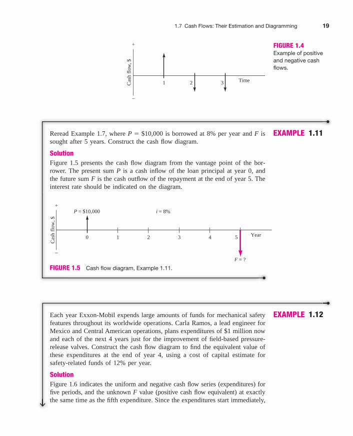
EXAMPLE 1.11

0

F = ?

+

–

5432

i = 8%

1 Year

P = $10,000

Cas

h fl

ow, $

FIGURE 1.5 Cash flow diagram, Example 1.11.

Reread Example 1.7, where is borrowed at 8% per year and F issought after 5 years. Construct the cash flow diagram.

SolutionFigure 1.5 presents the cash flow diagram from the vantage point of the bor-rower. The present sum P is a cash inflow of the loan principal at year 0, andthe future sum F is the cash outflow of the repayment at the end of year 5. Theinterest rate should be indicated on the diagram.

P � $10,000

EXAMPLE 1.12Each year Exxon-Mobil expends large amounts of funds for mechanical safetyfeatures throughout its worldwide operations. Carla Ramos, a lead engineer forMexico and Central American operations, plans expenditures of $1 million nowand each of the next 4 years just for the improvement of field-based pressure-release valves. Construct the cash flow diagram to find the equivalent value ofthese expenditures at the end of year 4, using a cost of capital estimate forsafety-related funds of 12% per year.

SolutionFigure 1.6 indicates the uniform and negative cash flow series (expenditures) forfive periods, and the unknown F value (positive cash flow equivalent) at exactlythe same time as the fifth expenditure. Since the expenditures start immediately,

bLa01293_ch01_001-026 9/4/07 9:35 PM


0 1 2

A = $1,000,000

3

F = ?i = 12%

4 Year�1


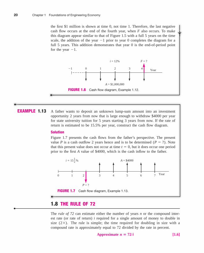
EXAMPLE 1.13

0 1 2

P = ?

7653

A = $4000

4 Year

i = 15 %12


1.8 THE RULE OF 72

The rule of 72 can estimate either the number of years n or the compound inter-est rate (or rate of return) i required for a single amount of money to double insize The rule is simple; the time required for doubling in size with acompound rate is approximately equal to 72 divided by the rate in percent.

Approximate [1.6]n � 72/i

(2�).

the first $1 million is shown at time 0, not time 1. Therefore, the last negativecash flow occurs at the end of the fourth year, when F also occurs. To makethis diagram appear similar to that of Figure 1.5 with a full 5 years on the timescale, the addition of the year prior to year 0 completes the diagram for afull 5 years. This addition demonstrates that year 0 is the end-of-period pointfor the year �1.

�1

A father wants to deposit an unknown lump-sum amount into an investmentopportunity 2 years from now that is large enough to withdraw $4000 per yearfor state university tuition for 5 years starting 3 years from now. If the rate ofreturn is estimated to be 15.5% per year, construct the cash flow diagram.

SolutionFigure 1.7 presents the cash flows from the father’s perspective. The presentvalue P is a cash outflow 2 years hence and is to be determined Notethat this present value does not occur at time but it does occur one periodprior to the first A value of $4000, which is the cash inflow to the father.

t � 0,(P � ?).

bLa01293_ch01_001-026 9/4/07 9:36 PM

1.9 Introduction to Using Spreadsheet Functions 21

For example, at 5% per year, it takes approximately years for a currentamount to double. (The actual time is 14.2 years.) Table 1.4 compares rule-of-72results to the actual times required using time value of money formulas discussedin Chapter 2.

Solving Equation [1.6] for i approximates the compound rate per year for dou-bling in n years.

Approximate [1.7]

For example, if the cost of gasoline doubles in 6 years, the compound rate isapproximately per year. (The exact rate is 12.25% per year.) Theapproximate number of years or compound rate for a current amount to quadru-ple (4�) is twice the answer obtained from the rule of 72 for doubling the amount.

For simple interest, the rule of 100 is used with the same equation formatsas above, but the n or i value is exact. For example, money doubles in exactly12 years at a simple rate of per year. And, at 10% simple inter-est, it takes exactly years to double.

1.9 INTRODUCTION TO USING SPREADSHEET FUNCTIONS

The functions on a computer spreadsheet can greatly reduce the amount of handand calculator work for equivalency computations involving compound interest andthe terms P, F, A, i, and n. Often a predefined function can be entered into onecell and we can obtain the final answer immediately. Any spreadsheet system canbe used; Excel is used throughout this book because it is readily available and easyto use.

100/10 � 10100/12 � 8.33%

72/6 � 12%

i � 72/n

72/5 � 14.4

TABLE 1.4 Number of YearsRequired for Money toDouble

Time to Double, Years

Compound Rate, Rule-of-72

% per year Result Actual

5 14.4 14.2

8 9.0 9.0

10 7.2 7.3

12 6.0 6.1

24 3.0 3.2

bLa01293_ch01_001-026 8/4/07 7:03 PM

foundations of engineering economy edition chapter 1.pdf1 chapter 1 foundations of engineering...

Documents