NTIA Report 94-302

Foundations, Applications, and Assessment of Wavelets

David A. Sutherland, Jr.

U.S. DEPARTMENT OF COMMERCE Ronald H. Brown, Secretary

Larry Irving, Assistant Secretary

for Communications and Information

December 1993

iii

PREFACE

The views and opinions expressed in this report are those of the author and do not in any way represent an official position of the National Telecommunications and Information Administration or of the U.S. Department of Commerce. Programming and plotting software are mentioned in this report to adequately explain the presentation of wavelet function plots. In no case does such identification imply recommendation or endorsement by the National Telecommunications and Information Administration, nor does it imply that the software identified are necessarily the best available for this application.

v

CONTENTS

1. INTRODUCTION .................................................................................................... 1 2. WAVELET BASICS ................................................................................................ 4 2.1 Preliminaries ................................................................................................ 4 2.1.1 Integral Transforms ..................................................................... 4 2.1.2 The Fourier Transform ................................................................ 5 2.1.3 The Windowed Fourier Transform.............................................. 6 2.2 Wavelets ..................................................................................................... 8 2.2.1 Characteristics of Wavelet Functions.......................................... 8 2.2.2 The Continuous Wavelet Transform ......................................... 13 2.2.3 Time-Frequency Localization ................................................... 14 2.2.4 Frames and the Discrete Wavelet Transform............................ 18 2.2.5 Orthonormal Wavelet Bases With Compact Support ............... 20 2.2.6 Introduction to Multiresolution Analysis .................................. 20 2.2.7 Determining Orthonormality of Wavelets................................. 31 2.2.8 Approximation Qualities of Wavelets....................................... 32 3. TELECOMMUNICATIONS ISSUES ................................................................... 41 3.1 Signal Processing....................................................................................... 33 3.1.1 Filter Banks and Wavelets......................................................... 33 3.1.2 Multiresolution Analysis in Two Dimensions .......................... 34 3.2 The Human Hearing System and Wavelets............................................... 37 3.3 Wavelet Packets and Compression............................................................ 39 4. NON-TELECOMMUNICATIONS APPLICATIONS.......................................... 41 5. SUMMARY ........................................................................................................... 42 6. CONCLUSIONS AND RECOMMENDATIONS ................................................. 43 7. REFERENCES ....................................................................................................... 45 8. BIBLIOGRAPHY................................................................................................... 49 APPENDIX ................................................................................................................. 50

1

FOUNDATIONS, APPLICATIONS, AND ASSESSMENT OF WAVELETS

David A. Sutherland Jr.∗

This report is an introduction to wavelet theory intended for the technical professional working in telecommunications. The basics of wavelet theory are presented with an emphasis on explanation of the principles and ideas involved rather than on the mathematical proofs. Differences between the wavelet transform and the windowed Fourier transform are pointed out. Wavelet applications to several issues important to telecommunications are presented.

Keywords: filter bank; filters; harmonic analysis; signal processing; time-frequency

methods; wavelets; wavelet transform; windowed Fourier transform

1. INTRODUCTION The purpose of this report is to introduce the subject of wavelets to the engineer, scientist, or technical specialist working in telecommunications. The report presents the ideas and the basics of wavelet theory without subjecting the reader to very much mathematical rigor. In fact, this paper presents only one formal mathematical proof (for the sake of illustration), handwaves a few other proofs, and states many results without proof. In each case, reference is provided for further research and reading. A bibliography for further reading is also provided. A major goal is to present information necessary for the telecommunications specialist to decide if further investigation of wavelets and their applications is warranted. It is not assumed that the telecommunications specialist is necessarily knowledgeable about any of the subjects to which wavelet theory is applied, such as digital signal processing, image processing, harmonic analysis, and real analysis. Such experts should delve into the literature listed in the references and bibliography directly. This report concentrates on a short treatment of the mathematical basics of wavelet theory. The reader should be familiar with Fourier analysis as is usually gained at the baccalaureate level for electronics engineers or as may be found in Spiegel (1974), Hsu (1984), or Chui (1992). The report concentrates on general characteristics of wavelets with an emphasis on the differences between wavelets and the long-established Fourier transform theory, and specifically the windowed Fourier transform. A few issues and aspects that directly pertain to telecommunications are presented along with a short list of other areas in which there is interest and ongoing work in applying wavelets. ∗ The author is with the Institute for Telecommunication Sciences, National Telecommunications and Information Administration, U.S. Department of Commerce, 325 Broadway, Boulder CO 80303.

2

The presentation on wavelets is limited to real functions. The discussion can also be extended to complex wavelet functions. The subject can be considered a subset of harmonic analysis (interested readers should consult the references or bibliography). Wavelets are families of functions which are written

.)( 21

, ⎟⎠⎞

⎜⎝⎛ −

= −

abxaxba ψψ (1)

Thus, the family {ψa,b} is generated by dilations and translations of the single function ψ. This function is called the analyzing wavelet, the basic wavelet, or the mother wavelet in the literature. The wavelet coefficients of a function are determined by the inner product in L2(R) of the members of the family and the function in question. The function can then be reconstructed from the wavelet coefficients. Dilation, translation, L2(R), and its inner product will be defined shortly. An example of a wavelet is the Haar function (Figure 1), which is defined

The Haar wavelet is not a very useful wavelet as an analysis tool, but it is often used (as it is here) for illustrative purposes. Haar discovered these "wavelets" around 1910. It has been known since then that the family of wavelets generated by the Haar function is an orthonormal basis of L2(R) (this fact will be proved using a wavelet analysis technique later) (Daubechies, 1992). Dilation and translation have been referred to as the "Haar processes" of "squeezing by one half" and "shifting" in the literature of Walsh and other orthogonal functions (Harmuth, 1972). In the mid 1980s, wavelets were used in research in seismic analysis, mainly in France. The French researchers led by J. Morlet, a geophysicist; Alexander Grossman, a physicist; and Yves Meyer, a mathematician, coined the name ondelettes (wavelets) and built strong initial mathematical foundations (Rioul and Vetterli, 1991). This generated the strong, recent interest in wavelets which has been fueled by more and more new applications of wavelets to other diverse fields.

3

Figure 1. The Haar wavelet. The interest in wavelets is due to increased time-frequency localization which wavelets provide in certain instances. That is, a wavelet analysis may provide increased resolution of a signal in comparison to Fourier techniques. The windowed Fourier transform (the short-time Fourier transform or the Gabor transform) also attempts to provide increased time-frequency resolution. Wavelets can also be considered a subset of time-frequency signal, representation methods which attempt to characterize a signal over a time-frequency plane or a combination of the time domain and the frequency domain. A wavelet analysis provides a time-scale representation with the scale representing a frequency band or octave. Specifically, wavelets are one of the linear time-frequency representations of which the windowed Fourier transform is also a member (Hlawatsch and Boudreaux-Bartels, 1992).

4

2. WAVELET BASICS This section of the report contains the elementary ideas on wavelets. It is intended to give the reader a basic foundation of the subject and should be considered introductory.

2.1 Preliminaries This section of the report covers the elementary ideas of Fourier analysis, especially the windowed Fourier transform. It is not intended to be complete but contains the ideas important to the foundations of the wavelet transform. 2.1.1 Integral Transforms A transform is an explicit operation, T, on a function, g(x), for example, which leads to another function, ĝ(s), that is, { } ),(ˆ)( sgxgT = (3) where s is the transform variable. The idea is that the value of ĝ(s) depends on the whole of g(x) and not on any single value of g(x) at a particular value of the independent variable, x. An integral transform involves integration over x. For example, take .0,)( >= − aexg xa (4) Let T be the operation (transform) defined by the two following steps: 1. Multiply g(x) by .2 sxie π− (5) 2. Integrate the product over x on the real line, (-∞, ∞). The result is

5

∫∞

−∞=

−−=x

sxixa dxeesg π2)(ˆ (6)

( )

.2

222 sa π+

=

This operation is obviously the familiar Fourier integral transform. It is also the inner product, in L2(R), written ., 2 sxixa ee π−− (7)

If a = 1, then the value of ĝ at s = 3.5 is 0.004127. This value depends on the whole of g(x). That is, ĝ(3.5) does not depend on any single value of g(x) at a particular value of x (Bracewell, 1990). Electrical and electronics engineers are usually familiar with the discrete and continuous versions of the Fourier transform, the Laplace transform, the Z transform, and the Hilbert transform. There are many other useful integral transforms (Bracewell, 1990). I will not dwell on general transforms except to note that the transforms discussed in this report are linear, that is, for functions g1(x) and g2(x), and constants a and b, { } { } { } ,)()()()( 2121 xgbTxgaTxbgxagT +=+ (8) which means that the superposition principal applies. 2.1.2 The Fourier Transform The Fourier transform represents the frequency content of a signal (function) g(t) over all time. Time, t, is the continuous independent variable of the signal. The Fourier transform of a function, g(t), is defined for the remainder of this paper as

∫∞

−∞=

−=t

ti dtetgg .)(21)(ˆ ω

πω (9)

The unit of ω is cycles per unit time which represents a temporal frequency. The unit of ω can be cycles per unit length if the independent variable of g is length rather than

6

time. Thus ω can represent a spatial frequency. The Fourier transform translates a function (signal) in the time domain to a function in the frequency domain. The Fourier transform is a one-to-one mapping from the real line, R, onto itself. An interpretation of the Fourier transform of a signal, g(t), is that it is the inner product of g(t) with sine wave basis functions defined on the entire real line. The Fourier transform, therefore, works well if the signal is made up of a few stationary components. A stationary signal is one whose statistical properties do not evolve in time; hence, a periodic signal is stationary. But the Fourier transform will not work as well if the signal has non-stationary components. Any sharp transitions in a signal over time will be spread out over the entire frequency axis of ĝ(ω). Such sharp transitions are, for example, noise, spikes, and other high-frequency, short-lived components. These transitions are localized in time and thus are non-stationary (Rioul and Vetterli, 1991). 2.1.3 The Windowed Fourier Transform The windowed Fourier transform looks at a non-stationary signal through a window so that the signal is approximately stationary in the window. This attempts to introduce time dependency (time localization) to the Fourier analysis. The windowed Fourier transform is defined as

( )( ) ∫∞

−∞=

−−=s

siwin dsetsgsftfT .)()(, ωω (10)

The windowed Fourier transform in its discrete form is defined by letting t=nt0, and ω=mω0, where m and n are integers, and t0 and ω0 are positive and fixed. The discrete windowed Fourier transform is defined as ( )( ) ∫ −−= .)()( 0

0, dsentsgsffT simwinnm

ωω (11) In both cases, (10) and (11), f(t) is the signal (function). The signal is multiplied by the windowing function, g(t) or g(t-t0). The windowing function, g, generally has compact support and has reasonable smoothness. Specifically, the windowing function must tend to zero quickly. A useful example for g(t) is a Gaussian with the tails chopped beyond 3σ. Equation (10) can be interpreted as the frequency content of f(t) near a specific value of t. Hence, the windowed Fourier transform describes f(t) in the time-frequency plane. That

7

is, the windowed Fourier transform maps the one-dimensional representation of a signal to a two-dimensional representation in time and frequency. The windowed Fourier transform is also known as the short time Fourier transform (STFT) or the Gabor transform. Figure 2 illustrates the construction of the argument of the windowed Fourier transform. The transform computes the Fourier coefficients for the product f(t)g(t). This is repeated for translated versions of the windowing function, i.e., g(t-t0), g(t-t1), ... .

Figure 2. The argument of the windowed Fourier transform. Another interpretation is that the windowed Fourier transform is a modulated filter bank. That is, equation 10 filters the signal over t with a bandpass filter at a given frequency, ω. This filter has as impulse response the window function, g(t), modulated to that frequency (Rioul and Vetterli, 1991). The time-frequency resolution of the windowed Fourier transform is fixed over the time-frequency plane since the same window is normally used for all frequencies. In fact, the product of the two resolutions is lower bounded, that is,

,41π

ω ≥∆∆ t (12)

where ∆ω is the frequency resolution and ∆t is the time resolution. Two frequencies cannot be resolved by the windowed Fourier transform unless they are more than ∆ω

8

apart. Likewise two pulses cannot be resolved unless they are more than ∆t apart. Equation 12 indicates that increased resolution in frequency is bought only with decreased resolution in time and vice versa. Note that if the windowing function, g(t), is a Gaussian, then the lower bound expressed in (12) is an equality (Rioul and Vetterli, 1991). Examples of other windowing functions and their characteristics can be found in the signal processing literature; see, for example, Harris (1978).

2.2 Wavelets The basic ideas of wavelets are covered in this section. Discrete and continuous wavelets are covered. Time-frequency resolution of the windowed Fourier transform and of the wavelet transform are discussed in enough detail to make the differences clear and a theorem introducing multiresolution analysis is presented in detail. The theorem is illustrative of the process of wavelet analysis and the characteristics of wavelet bases and wavelet functions. Multiresolution analysis is an important development of wavelets and is based on previous work in video decomposition (Burt and Adelson, 1983). 2.2.1 Characteristics of Wavelet Functions Generating L2(0,2π) and L2(R) L2(0,2π) is the set of all measurable (piecewise continuous) functions, f, defined on the interval (0,2π) in R such that

∫=

∞<π2

0

2 .)(x

dxxf (13)

Any function f ∈ L2(0,2π) can be extended periodically to the real line by defining )2()( π−= xfxf (14) for all x ∈ R. This function space is generated by the basis {einx}. This basis is the set of integer dilations of f(x)=eix. The spaces L2(0,2π) AND L2(R) are different. In particular, a function in the latter satisfies

9

∫∞

−∞=

∞<x

dxxf .)( 2 (15)

The space L2(R) is the set of all measurable functions (again, piecewise continuous) that satisfy (15); that is, they are square integrable. Another interpretation of L2(R) is that it is the space of one-dimensional signals with finite energy. It is clear from (15) that the {einx} basis functions of L2(0,2π), sines and cosines (waves), do not belong to L2(R). Are there waves or wavelike functions that do belong to L2(R) that can be used to generate the space? If they exist, it is clear again from (15) that such a wavelike function must decay or go to zero fairly quickly (this is one explanation for the use of the term "wavelet," as a little or small wave). To get the wavelike function to cover all of the real line it is now necessary to translate (shift) our function over the real line. To cover all "frequencies" like the basis {einx} does for L2(0,2π) we must dilate and contract our function. The result is that we do not have single frequency waves, but waves that partition frequencies into frequency bands (octaves). The demonstration of a wavelet basis for L2(R) will be taken up in a later section of this report. The norm of a function f(x) ∈ L2(R), indicated by ||f||, is the square root of the inner product of the function with itself or

Dilation A dilation of a function, f(x), is another function g(x)=f(kx) where 0<k<1. This has the effect of "spreading" the function out over its domain. A contraction, the opposite of dilation, of a function has k>1. The action of a contraction is "squeezing" the function over its domain. For example, let ψ be the Haar wavelet defined in (2). Then, a dilation of the Haar wavelet, k=1/2, is

10

while a contraction of the Haar wavelet, k=2, is

Dilations and contractions are used to change the basic wavelet (mother wavelet) to another scale. That is, by dilation and contraction, a wavelet analysis can partition a signal (or function) into "frequency bands" or octaves determined by scale, rather than into single frequencies as does a Fourier analysis. The scale parameter is most often 2 (binary dilation and contraction), but other scale parameters are also possible. Binary dilations of the mother wavelet can then be indexed by the integers, that is

where j ∈ I. In Section 2.2.3 I take up the advantages of this partitioning to time-frequency resolution offered by wavelets and in Section 2.2.6, I offer an example of such a partitioning. Translation A translation of a function, f(x), is another function, g(x)=f(x-k) which has the effect of moving the function, shifting f(x), to the right, if k is positive. If k is negative, the function is translated to the left. Translations of wavelets are generally translations by dyadic rationals (this means that the numerator and denominator are determined by separate indices). This is necessary to ensure that the entire real line is covered even when the scale changes. For example, consider

11

( )kxj −−2ψ (20) where k and j are both integers. Note that -j indexes both the dilation factor, 2-j and the denominator of the dyadic translation, k/2-j (in terms of the notation used in (1), a=2j and b=k2j). This guarantees that successive translations, k increased or decreased by one, are adjacent and leave no uncovered gaps in the real line. Notice that all wavelets in a family (defined by a basic or mother wavelet) can be indexed by scale and translation. Section 2.2.6 gives a detailed example of translation and dilation indexing in a wavelet analysis. Definition of a Wavelet A wavelet is a function, ψ(x) ∈ L2(R), such that ( ) ,ˆ

21 ∞<∫− ξξψξ d (21)

which is known as the admissibility condition. This implies that with sufficient decay at infinity ∫ = .0)( dxxψ (22) A single wavelet generates a wavelet family (later a wavelet basis or a frame) by the formula

( ) .22 2, kxj

j

kj −= −−

ψψ (23) Note that ., ψψ =kj (24) For wavelets in a particular class (which we shall investigate later) there exists a scaling function φ(x) which corresponds to ψ(x). Several necessary properties or conditions on wavelets can be analyzed in terms of the scaling function and will be taken up in later sections. The Scaling Function A basic wavelet can be defined in terms of a scaling function. For example, the Haar wavelet (2) can be written in terms of the scaling function φ(x) by

12

)12()2()( −−= xxx φφψ (25) where

which is the scaling function associated with the Haar wavelet. The scaling function is not necessarily unique for any wavelet. The scaling functions for each separate scale, j, are determined by the recursive relationship

∑∞

=− −=

01 ,)2()(

kjkj kxcx φφ (27)

where φ0 is given by (26), and where the recursive coefficients, ck's, are not trivially determined. Note here that only finitely many of the ck's are non-zero. Determining the ck's will not be taken up in this report. See, for example, Daubechies (1992) or Strichartz (1993). Wavelets are defined recursively. Therefore, except for the Haar wavelets, a wavelet cannot be defined in closed form. The problem with wavelets here is that their distinct properties cannot be determined directly, but only indirectly by dealing with the recursion relationships, specifically the recursion coefficients that define the scaling function (27) and that define the wavelets at the same scale as φj by ∑ −−= −

kjk

kj kxcx .)2()1()( 1 φψ (28)

Thus, in practice, an individual wavelet in the wavelet family is defined in terms of the scaling function at the same scale as the wavelet and the scaling function is defined in terms of the scaling function φ0 that is associated with the mother wavelet ψ(x). It is clear that everything is determined by the scaling function and the recursion coefficients. More on the scaling function is discussed in later sections. This property of definition by recursion is one reason that wavelets receive much attention as there are many ways to accelerate the recursive process to do the necessary computations. Strang (1989) even refers to wavelets as "recursion heaven."

13

Equations 27 and 28 indicate that wavelets and the associated scaling functions have a self-similar nature due to the processes of recursive definition. 2.2.2 The Continuous Wavelet Transform A method of getting increased resolution in both time and frequency is the "constant Q analysis," where Q stands for quality factor. The main feature here is that frequency resolution is proportional to the frequency or

.c=∆ωω (29)

In constant Q analysis there is a filter bank with constant relative bandwidth, i.e., where c is constant. Instead of a single filter, as in the windowed Fourier transform, the bandwidth of each one of the bandpass filters, or windowing functions, in the bank is proportional to its central frequency. The bandpass filters in a constant Q analysis do not necessarily have to be similar or related. The wavelet transform does the same type of windowing analysis as a constant Q approach except that all the filters are related. In fact, they are scaled and translated versions of the same function, called the mother wavelet or the analyzing wavelet (or just plain wavelet). The continuous wavelet transform is

( )( ) ( )∫ ⎟⎠⎞

⎜⎝⎛ −

= − dta

bttfabafT wav ψ21

, (30)

where a,b are real, a≠0, and ψ is the mother wavelet or analyzing wavelet. The functions

⎟⎠⎞

⎜⎝⎛ −

= −

abtaba ψψ 2

1

, (31)

are wavelets, as in little waves. The mother wavelet or analyzing wavelet is ψ1,0. The family {ψa,b} is generated by the mother wavelet. At this point the family {ψa,b} is assumed to be a suitable basis of L2(R). The mother wavelet is also referred to as the generating wavelet since it generates a basis. Note the similarity of (30) with the windowed Fourier transform, (10). Both are inner products of a signal (function) with a set of doubly indexed functions.

14

To recover f, the reconstruction formula for (30) is given by

( )∫∫∞

−∞=

∞

−∞=

−=b

bawav

a adadbfTCf 2,

1 ψψ (32)

where ( )∫

−= .ˆ2 21 ξξψξπψ dC (33) Equation 33 must clearly be bounded, see (21), for (32) to make any sense. So, equation 33 is known as the admissibility condition. Proof of (32) can be found in Daubechies (1992) or Chui (1992). 2.2.3 Time-Frequency Localization It has already been indicated that wavelets give increased time-frequency resolution, whereas the windowed Fourier transform is limited by an uncertainty relationship. This is explained in more detail here; even further details can be found in Chui (1992) or Daubechies (1992). The windowed Fourier transform attempts to introduce time localization to signal analysis. Notice that (10) is a function of both time and frequency. The transform maps the signal from the time domain (the real line) to the time-frequency plane (phase space). However, as mentioned before, time and frequency resolution of the windowed Fourier transform is fixed since that same window is used for all frequencies. This can be seen in the following. The Gaussian is the optimal window for time-frequency resolution since (12) is an equality for a Gaussian. Note also that the Fourier transform of a Gaussian is another Gaussian. The general Gaussian is

,2

1)( 4

2

αα πα

t

etg−

= (34)

where α is a fixed and positive constant. It can be shown that the width, RMS duration, of the Gaussian window function is α½, see Chui (1992). The form of the windowed Fourier transform (10) is then

15

( )( ) ( ) ( ) .)(, dtbtgtfefTt

tiwinba −= ∫

∞

−∞=

−α

ωω (35)

This is interpreted as the localization of the Fourier transform of f(t) around time b by the windowing function gα(t). If we let ,)()(,, btgetG ti

b −= αω

ωα (36) then (35) becomes

( )( ) .)()( ,,, dttGtffT bt

winba ωαω ∫

∞

−∞=

= (37)

Note that (37) is the inner product ., ,, ωα bGf (38) Now, by invoking Parseval's identity

,ˆ,ˆ21, ,,,, ωαωα π bb GfGf = (39)

which relates inner products of L2(R) functions with the inner products of their Fourier transforms, we arrive at

So, the windowed Fourier transform of f(t) at window width α½ centered at t=b is equal to the windowed inverse Fourier transform at window width (α/4)½ centered at η=ω (up

16

to the leading coefficient). Hence, the frequency window is also fixed for every central frequency. Time-frequency resolution is illustrated by Figure 3.

Figure 3. Time-frequency resolution of the short-time Fourier transform. Our conclusion is that the time-frequency window is fixed for any choice of central frequency and for any choice of time. The implication is that the windowed Fourier transform is not useful in situations where it is necessary to analyze high and low frequencies at the same time. Now show that the time-frequency window is not fixed for the wavelet transform. The general wavelet is again defined as

.)( 21

, ⎟⎠⎞

⎜⎝⎛ −

= −

abtatba ψψ (41)

And the wavelet transform of a signal (function), f(t), is

17

∫ ⎟⎠⎞

⎜⎝⎛ −

= − ,)(, 21

dta

bttfaf ψψ (42)

where f(t) ∈ L2(R). Assume that both ψ and its Fourier transform are window functions, that is tψ(t) ∈ L2(R) and ωψ̂ (ω) ∈ L2(R). This assumption has the appearance of handwaving. But not every wavelet meets this criteria. For example, the Fourier transform of the Haar wavelet does not fall off to zero quickly enough and hence cannot be a window function. The assumption is necessary to keep this discussion general for wavelets. For a detailed discussion see Daubechies (1992). Note that this is automatic for the Gaussian windowed Fourier transform. By applying Parseval’s identity we have

( ) .ˆˆ2

,21

ωωψπ

ψ ω daefaa

f ib∫ −

−

= (43)

The Fourier transform of ψ(aω) is a window function with radius

ψ̂1∆

a (44)

and center frequency ω* / a, where ψ̂∆ (45) is the radius of the Fourier transform and ω* is the center frequency of the original wavelet (Chui, 1992). If we now consider the window as a filter with a center frequency of ω* / a and a bandwidth twice (44), then the ratio of the center frequency to the bandwidth is given by

.2

*

ψ̂

ω∆

(46)

Notice that this is independent of the center frequency of the window. This is basically constant-Q filtering. Hence, the time window narrows for high-frequency analysis and

18

widens for low-frequency analysis because of the uncertainty relationship (12). This is illustrated graphically in the time-frequency plane in Figure 4.

Figure 4. Time-frequency resolution of the wavelet transform. It must be pointed out that constant-Q filtering is a development of Fourier analysis; it is not exclusive to wavelet analysis. Constant-Q filtering can be accomplished by varying the α parameter in (34). The resulting windows are not necessarily scaled or translated versions of a basic Gaussian (however, they can be). In fact, windows for high and low frequencies may be totally different functions altogether. In a wavelet analysis, all the windows are scaled and translated versions of one function, the mother wavelet. 2.2.4 Frames and the Discrete Wavelet Transform The discrete wavelet transform comes from the continuous wavelet transform (30) by discretizing the two parameters a and b. Let a = a0

m, where m is an integer and a0 ≠ 1. The most "natural" choice for the dilation parameter is to set a0 = 2, although this is by no means the only choice. For the translation parameter, b, we must make sure to relate it to a0 so that the real line is covered as in 2.2.1. So let b = nb0a0

m where b0 > 0. Note that both m and n range over the integers. Hence, we have the discrete wavelet transform

19

( ) ( ) ( )∫ −= −− ,002

0, dtnbtatfafW mm

wavnm ψ (47)

which is just the inner product nmf ,,ψ (48) in L2(R). The question now is whether these coefficients, from (47), completely characterize f. Or equivalently, can f be completely reconstructed from the coefficients (47)? The answer is yes, if the {ψm,n} is an orthonormal basis of L2(R). But, the wavelet basis does not necessarily have to be orthonormal. Nor does the family {ψm,n} have to be a basis at all. The condition is that the {ψm,n} must constitute a frame. The family {ψm,n} is a frame in L2(R) if for all functions, f ∈ L2(R), there exist real numbers, A > 0 and B < ∞, such that ., 22

,,

2 fBffAnm

nm ≤≤ ∑ ψ (49)

This is an admissibility condition for the discrete wavelet transform. If A = B the frame is called a tight frame and if A=B=1 the frame is an orthonormal basis of L2(R). In the case that A=B the number is called the redundancy ratio, which is the ratio of frame vectors to the basis vectors of the space (Heil and Walnut, 1989). The frame does not necessarily have to be a basis and in fact the frame does not necessarily have to be linearly independent. This implies that uniqueness of representation is lost. Nevertheless, recovery is numerically stable. Frames are useful in situations in which orthonormal bases can’t be used or in which conditions on the functions being analyzed make orthonormal bases unwieldy. Note that the idea of frames is not new and that in fact the notion of frames is also used in Fourier analysis; specifically, it can be used to create orthonormal bases for the windowed Fourier transform (Daubechies, 1992). A specific formula exists for exact reconstruction of f from the coefficients in terms of a discrete inverse wavelet formula, which is ∑=

nmnmnmff

,,,

~, ψψ (50)

20

where the kernel function of the inverse formula (or the dual of ψ) is indicated by the tilde. There are problems with the dual in that it also must generate a wavelet family which constitutes a frame. Another problem is that the dual might not be in L2(R). 2.2.5 Orthonormal Wavelet Bases With Compact Support An orthonormal basis of functions of L2(R) is useful for several reasons. The L2(R) functions can be represented by a linearly independent set of basis functions uniquely. With an orthonormal basis, the expansion coefficients may be computed by use of the inner product for L2(R). The alternative is to compute the coefficients by a large system of equations which could be very time consuming (Alpert, 1992). An orthonormal basis is also stable. This is extremely important in numerical representation of functions. The idea is that if the coefficients of the representation of a function are perturbed then the function itself is perturbed the same amount and vice versa. This is important since numerical representations are truncated; that is, computers can only represent real numbers to finite precision (Alpert, 1992). A method giving an orthogonal decomposition of subspaces of L2(R) is important for multiresolution analysis. This will be taken up in the next section. Compact support is desirable in signal processing to avoid distortion in compression. Basically, a reconstructed signal which is the result of linear filtering will avoid distortion if the filter has linear phase (Rioul and Vetterli, 1991). Daubechies (1988) has discovered a family of orthonormal wavelet bases with compact support. The Haar function is the first member in the family. Of this family, the Haar function is the only one that has a closed form solution. The properties of the other wavelets in the family may only be observed indirectly. An example of this is given in section 2.2.7 which gives a method to determine the orthonormality of a general wavelet. Other members of the Daubechies family of wavelets are graphically displayed in the Appendix along with their filter coefficients. 2.2.6 Introduction to Multiresolution Analysis Multiresolution analysis is a method of analyzing a signal at different scales, and hence is also referred to as multiscale approximation. Multiresolution analysis is probably the most significant development in the work on wavelets. It has application to pattern recognition (in artificial intelligence), image compression, and signal analysis and detection. Nevertheless, the ideas aren’t new since multiresolution analysis is a further development and refinement of the Laplacian pyramid scheme of Burt and Adelson (1983).

21

The simplest of wavelet functions is the Haar function, or Haar wavelet (2). The Haar function is widely used for illustrative purposes, but it is not a very useful analysis tool. I will use the Haar wavelet to present an illustrative proof of a theorem from Daubechies (1992) which is rich in the basic ideas of wavelets, uses wavelets as an analysis tool, and introduces the basic concept of multiresolution analysis. The family of wavelets with the Haar function (2) as the generating wavelet is defined by

( ) ,22 2, kxj

j

kj −= −−ψψ (51)

where j and k are integers and ψ is the Haar wavelet. Here j is the scale factor and k is the translation factor. The scale factor operates on the integer 2, the dilation factor. This is not the only choice for the dilation factor, by any means, although it is convenient. The subscripts, j and k, and the dilation factor characterize the individual wavelets. THEOREM: The family of functions, {ψj,k}, as defined by (51) and with the Haar Wavelet as the mother wavelet is an orthonormal basis of L2(R). PROOF: The first task is to show that the ψj,k are indeed orthonormal. That is, show that

The left side of (52) is the inner product in L2(R) and is given by

∫∞

−∞=′′

xkjkj dxxx .)()( ,, ψψ (53)

Suppose the scale is the same, j=j′. Then, if the translation is the same, k=k′, we have

∫∞

−∞=

=x

kj dxx .1)(2,ψ (54)

(The poor readers are left to fend off the ugly integrations for themselves). If the translation is not the same, k≠k′ (scale still the same), then the two wavelets do not overlap. And since each wavelet equals zero on the support of the other, their product is zero.

22

Now suppose that the scale is not the same, j≠j′. If the wavelets do not overlap, then their product is zero as above. If the wavelets do overlap we have the situation below in Figure 5.

Figure 5. Overlapping wavelets of different scale-Haar mother wavelet. The product of these two wavelets is just the smaller-scale wavelet times a constant (the constant amplitude of the larger-scale wavelet). The integral of the product is proportional to the integral of the smaller-scale wavelet, which is zero, see (21) and (22). Hence, the family of wavelets, {ψj,k}, is orthogonal. Orthonormality follows from the fact that the square root of the norm of any of the ψj,k’s equals one. The second task is to show that any function f′ ∈ L2(R) can be arbitrarily approximated by a finite linear combination of members of {ψj,k}. That is, I must show that given ε>0

,,, εψ <−′ ∑∑ kjkjkj

Cf (55)

where the j’s and k’s are bounded (note here that the double summation in (55) is called a wavelet series) and • indicates the norm for L2(R) given by (16). Recall that L2(R) can be interpreted as the space of square integrable functions characterized by (13.). Thus, the second task is to show that a signal with finite energy can be arbitrarily

23

approximated by a finite linear combination of the members of {ψj,k} which are also in L2(R). It is known that f′ can be arbitrarily approximated by a function, f, with compact support, which is piecewise constant on the intervals [ℓ2-m,(ℓ+1)2-m) where ℓ,m∈I. The function, f, is simply a step function with step width of 2-m. The integer, ℓ, indexes the intervals of width 2-m. Therefore, we can find an f such that

.2ε

<′− ff (56)

Then, by showing that

,2,,εψ <−∑∑

j kkjkjCf (57)

and by invoking the triangle inequality, we have

.

22

,,,,

εεε

ψψ

=+<

−+′−≤−′ ∑∑∑∑j k

kjkjj k

kjkj CfffCf (58)

We have introduced a step function, f, that arbitrarily approximates f′. Thus the task, proving (58), is to show that the finite linear combination of members of {ψj,k} arbitrarily approximate f. So, let f be supported on [-2M′,2M′] and be piecewise constant on the intervals, [ℓ2-M,(ℓ+1)2-M), where M and M′ are positive integers. The integer ℓ indexes the intervals of which there are M+M′+1. Let f0=f. And let fℓ0=f0 on the interval [ℓ2-M,(ℓ+1)2-M). The basic process is to decompose f0 into two parts, ,110 δ+= ff (59) where f1 is the same type of function as f0, but with step width 2-M+1, that is, the step width of f1 is twice as long as that of f0. The δ1’s represent the fine level of detail that is subtracted from f0 to get f1. The new step function, f1, approximates f1 on the intervals [n2-M+1,(n+1)2-M+1). Define fn

1= f1 on the interval [n2-M+l,(n+1)2-M+1) and let

.2

012

021 ++

= nnn

fff (60)

24

So, the fn1’s are determined by the process of averaging consecutive fℓ0’s which is

illustrated in Figure 6.

Figure 6. Averaging process. Hence, f1 is the average of f0 over the intervals [n2-M+1,(n+1)2-M+1). Notice that f1 is a fuzzier (more blurred) or less detailed approximation of f′ than f0 since the high frequency information has been taken out of f0. This "filtering" process is illustrated in Figure 7. The function, δ1, is also piecewise constant, as is f0, on the intervals [ℓ2-M,(ℓ+1)2-M), and has the same step size as f0. So, δ1 must be subscripted the same as f0. The sum of the pair δ2n

1, δ2n+11 is just a translated and scaled version of the Haar wavelet (2), the mother

wavelet, and so is one of the ψj,k’s, since

( ) ,21 0

120

210

212 +−=−= nnnnn ffffδ (61)

and

( ) .21 1

20

20

1210

121

12 nnnnnn ffff δδ −=−=−= +++ (62)

Note here that 2n=ℓ.

25

Figure 7. Reduction of detail. So, δ1 can be written as the sum

( )ll

l

−= −

+−=∑

−+′

−+′

xMMM

MM

112

2

12

1 21

1

ψδδ (63)

or in a more compact and convenient notation ∑ +−+−=

lll .,1,1

1MMC ψδ (64)

And, f0 can now be written as ∑ +−+−+=

lll .,1,1

10MMCff ψ (65)

The same process can be applied to f1, which leads us to

26

∑ +−+−+=l

ll .,2,221

MMCff ψ (66)

This second step is illustrated in Figure 8.

Figure 8. Second averaging process. This process is continued until the entire support of f, [-2M′,2M′], is covered, and we have

∑ ∑′

+=

′+ +=M

Mjjj

MM Cff1

,, ,l

ll ψ (67)

where .01

MMMMMM fff ′+′+−

′+ += (68) The constant function f-1

M+M′ is the average of f on the interval [-2M′,0), and f0M+M′ is the

average of f on the interval [0,2M′); see Figure 9.

27

Figure 9. The function fM+M′. We can continue the above decomposition process ,11 +′++′+′+ += MMMMMM ff δ (69) where

and

( ) ( ) .12212

21 1

11

0 +−= −−′+−

−−′+′+ xfxf MMMMMMMM ψψδ (71)

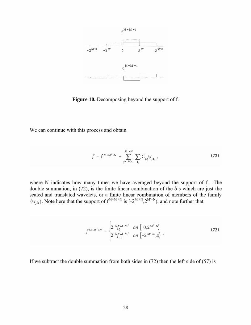
What has happened is that we have continued the averaging (decomposition) process beyond the support of f. There is nothing to stop us from taking the averages over the larger interval. This is illustrated in Figure 10.

28

Figure 10. Decomposing beyond the support of f. We can continue with this process and obtain

where N indicates how many times we have averaged beyond the support of f. The double summation, in (72), is the finite linear combination of the δ’s which are just the scaled and translated wavelets, or a finite linear combination of members of the family {ψj,k}. Note here that the support of fM+M′+N is [-2M′+N,2M′+N), and note further that

If we subtract the double summation from both sides in (72) then the left side of (57) is

29

By taking N large enough, this expression is as small as we want, which will satisfy (57) and in turn (58), which proves the theorem. This theorem is an introduction to multiresolution (multiscale) wavelet analysis. Each fm is contained in a subspace, Vm, m ∈ I, of L2(R). The subspace Vm is the space of all functions that are piecewise constant on the intervals [ℓ2-m,(ℓ+1)2-m). What a surprise! The spaces, Vm, are called a ladder of spaces and have the following properties:

Any sequence of subspaces of L2(R) which satisfy (75) is a multiresolution analysis. Note that these properties indicate that the Vm’s are just scaled versions of one space. Now for the real surprise! If there exists a sequence of subspaces of L2(R) that satisfy (75), then there exists a function φ∈ V0 such that φ0,k(x)=φ(x-k) is an orthonormal basis of V0, and the associated wavelet basis is an orthonormal basis of L2(R) (Mallat, 1989a). This function, φ, is called the scaling function of the multiresolution analysis (or the scaling function of the associated wavelet ψ), and is not necessarily unique. The scaling function is said to generate the multiresolution analysis. For the Haar wavelet, the scaling function is

30

Our mother wavelet can be described in terms of the scaling function as in (25). More generally the wavelet is defined by ∑ −−= +−

nn

n xx ,)12()1()( 1φαψ (77)

where the coefficients .,2 ,1 nn −= φφα (78) The Laplacian Pyramid Scheme Multiresolution analysis is an application and refinement of the Laplacian pyramid scheme of image encoding developed by Burt and Adelson (1983). This technique takes the original image, g(0), and applies an appropriate low pass filter. The result of the filtering operation, g(1), is subtracted from the original image. This difference, L(0), is encoded and, since it is largely uncorrelated, can be easily compressed by other techniques. The resultant image, g(1), is then subjected to the same filtering operation at a different scale. The result is the sequence L(0), L(1), L(2), L(3), ... , L(n). Note that the first element contains the high-frequency data, which is the most highly detailed information. Note also that the sequence g(0), g(1), g(2), ... , g(n-1) is a set of fuzzier and fuzzier (less detailed) versions of the original image. This set was called a "quasi-bandpass" copy of the original image and could be used directly, for example, for pattern recognition tasks. This Laplacian pyramid algorithm suffers from the fact that information at different levels is correlated. This leads to a significant question: Is similarity of adjacent detail images, L(i) and L(i+1) due to the redundant information added by the algorithm or is the similarity due to some property of the image? According to Mallat (1989c) this is not an easy problem to solve; however, it is crucial in pattern recognition. This Laplacian pyramid scheme is the same basic technique used in multiresolution analysis. It was first applied by Stephane Mallat (1989a), with an orthonormal wavelet basis. The advantage of using wavelets for such a scheme is that the orthonormality at each scale eliminates redundancy. This in turn results in eliminating the correlation between resolution levels.

31

2.2.7 Determining Orthonormality of Wavelets The orthonormality of the Haar wavelet basis can be determined directly since it is the only wavelet basis such that each member of the generated family can be described in closed form. For other wavelet bases, the individual wavelets can only be described recursively. In order to determine the orthonormality of a general wavelet we must use another approach. Start with the scaling function of the general wavelet (27) and take its Fourier transform,

⎟⎠⎞

⎜⎝⎛= ∑

−

2ˆ

21)(ˆ 2 ξφξφ

ξ

n

in

neh (79)

where the hn’s are filter coefficients, or the ck’s in (27), then rewrite it as

.2

ˆ2

)(ˆ 0 ⎟⎠⎞

⎜⎝⎛

⎟⎠⎞

⎜⎝⎛=

ξφξξφ m (80)

We then note a result from Daubechies (1992) that states that for every orthonormal family of functions, φ(x-n), in L2(R)

( ) .212ˆ 2

ππζφ =+∑

l

l (81)

Substitute (80) into (81) and we have

( ) ( ) .21ˆ 22

0 ππζφπζ =++∑ ll

l

m (82)

Note that ζ=ξ/2. If we now separate the summation of (82) into odd and even terms, and apply (81) while noting that m0 is periodic, we have

( ) ( ) ,120

20 =++ πζζ mm (83)

which is the condition we want. If (83) is satisfied then we have an orthonormal wavelet basis of L2(R). We note that this requires knowledge of the recursion coefficients, hn.

32

We have found a method to check for orthonormality. We note that some wavelet bases can be "made" into an orthonormal family by an orthogonalization trick. The formula in terms of the non-orthogonal scaling function is

( ) ( ) ( ) ,ˆ2ˆ21ˆ 2

12

ξφπξφπ

ξφ−

∗⎥⎦

⎤⎢⎣

⎡+= ∑

l

l (84)

where the original non-orthogonal family constitutes a Riesz basis. For details on Riesz bases consult Daubechies (1992) or Chui (1992). Basically, a Riesz basis (or an unconditional basis) is a basis which is a frame as well (Ruskai, 1992). 2.2.8 Approximation Qualities of Wavelets The approximation qualities of wavelets can be stated as follows: All polynomials of degree less than or equal to p-1 can be written as linear combinations of the translates of φ. Suitably smooth functions, functions for which the pth derivative exists, can be approximated with error O(hP) by linear combinations of the translates of φ-j such that

( ) ,22 )( pjp

k

jk fCkxaf ≤−−∑ −φ (85)

where h is the scale, 2-j. The first p moments of the wavelet ψ(x), associated with the scaling function φ(x), are zero, that is ∫ −== .1,...,0,0)( pmdxxxmψ (86) The wavelet coefficients of a suitable smooth function decay like C2-jp. These statements follow from a previously developed theory of translates which states that for accuracy hP, the Fourier transform of φ must have zeros of order p at all points ξ=2πn. This implies that m0, from (80), has a zero of order p at ξ=π (Strang, 1989; Daubechies, 1992; and Beylkin et aL, 1992).

33

3. TELECOMMUNICATIONS ISSUES This section covers a few applications of wavelets to issues important to telecommunications. The section on signal processing points out the strong connection of wavelets and finite impulse response filter theory and extends the ideas presented on multiresolution analysis to two dimensions which is important to video signal processing. Since audio signals are also important to telecommunications a brief section is included on the multiresolution analysis which is carried out by the human hearing system. And finally ideas which generalize the orthonormal wavelet bases are presented.

3.1 Signal Processing This section discusses the connection of wavelets to already known filter bank theory. It is pointed out that filter sequences which characterize wavelets are already known and characterized by workers in filter bank theory. They are quadrature mirror filters (or quadrature conjugate filters). An extension of multiresolution analysis to two-dimensional signals is also presented. 3.1.1 Filter Banks and Wavelets Finite impulse response filter bank theory includes orthogonal wavelet bases. In fact, orthonormal wavelet bases with compact support is a special case. While Daubechies was constructing her orthonormal wavelet bases with compact support, characterized by the finite sequences satisfying (89) and (90), workers in filter bank theory were characterizing the same sequences as two-channel perfect reconstruction quadrature mirror filter (QMF) banks (also known as conjugate quadrature filter (CQF) banks) (Gopinath and Burrus, 1992; and Vaidyanathan and Hoang, 1988). A filter bank can be thought of, simply, as a filtering of a signal by several filters in parallel followed by subsampling. A filter is a convolution operator. The sequence hn in (79) is called the scaling vector. The scaling vector determines the frequency decomposition of the discrete wavelet transform. The orthogonal properties of the scaling function and related wavelet function are determined by the scaling vector and follow from (79) (Gopinath and Burrus, 1992) by continuing to take Fourier transforms, that is

( ) .2

ˆ2

1ˆ1

2 ⎟⎠⎞

⎜⎝⎛

⎥⎥⎦

⎤

⎢⎢⎣

⎡= ∏∑

=

−

M

M

m n

in

nmeh ξφξφξ

(87)

34

In the limit (87) becomes

( ) ( )∏ ∑∞

=

−=

1

2

210ˆˆ

m n

in

nmehξ

φξφ (88)

which converges if .2=∑ nh (89) Now (89) and ,,02 kknn hh δ=∑ + (90) when satisfied by finite sequences hn (along with additional regularity assumptions; that is, the number of times the wavelet function is continuously differentiable) are the characterization of the family of orthonormal wavelet bases with compact support that was discovered by Daubechies and by Vaidyanathan in filter bank theory (Daubechies, 1992 and Vaidyanathan and Hoang, 1988). In filter bank theory, filters which satisfy (90) are called QMF’s or QCF’s. Lawton (1990) showed that any finite sequence hn satisfying (89) and (90) is a scaling vector that leads to a tight frame (a frame that is a basis) in L2(R). In fact, Lawton (1990) showed that almost all choices for the sequence hn lead to an orthonormal basis. From a filter bank point of view, these sequences are a two-channel (filter) perfect reconstruction filter bank (Vetterli 1992, Gopinath and Burrus 1992, with further reference to (Lawton, 1990). Very simply (and naively), the two channels (filters) are the scaling function (or scaling vector) and the wavelet (or wavelet vector). 3.1.2 Multiresolution Analysis in Two Dimensions There are several wavelet methods for decomposing a two-dimensional signal. Some of these methods are used in wavelet techniques of numerical analysis applied to matrix operations. Numerical methods and associated issues are not fully discussed in this report. These methods have application to image compression, two-dimensional digital signal processing, and pattern recognition. An analyzing wavelet for a two-dimensional multiresolution analysis in L2(R) can be created from the tensor product of two wavelet bases in L2(R). For example, if the wavelet functions in the one-dimensional basis are

35

( )kxx jj

kj −= −−22)( 2

, ψψ (91) then the corresponding wavelets in two dimensions are defined as ( ) ( ) .),( ,,,,, yxyx mlkjmlkj ψψψ = (92) A problem with this representation is that the variables are dilated separately. Perhaps a more useful approach is the following, which starts with a separable multiresolution decomposition of L2(R2) and produces three associated analyzing wavelets that together generate an orthonormal basis of L2(R2). Separability means that each of the subspaces can be decomposed as a tensor product of two identical subspaces of L2(R). Details can be found in Mallat (1989a). If the scaling function φ(x) generates a multiresolution analysis of L2(R), then a scaling function generating a multiresolution analysis of L2(R2) can be defined as ( ) ( ) ( ) ., yxyx φφ=Φ (93) This is technically the tensor product of the two one-dimensional multiresolution analyses. If ψ(x) is the wavelet defined by the scaling function φ(x), then

)()(

)()()()(

yxyxyx

d

v

h

ψψ

φψ

ψφ

=Ψ

=Ψ

=Ψ

(94)

are wavelets and generate an orthonormal basis of L2(R2). The superscripts h, v, and d are meant to be descriptive of horizontal, vertical, and diagonal spatial orientations. The multiresolution decomposition of a two-dimensional image is illustrated in Figures 11-13. The multiresolution decomposition of a white square on a black background is illustrated in Figure 14. If the coefficients of the scaling function φ and the wavelet ψ are considered as the coefficients of the QMF filters, H and G, respectively, in one dimension, then the decomposition process that leads to hi, for example, is

1. Applying the filter G to the rows of the image Ai, 2. Down-sampling the columns by a factor of 2,

36

37

3. Applying the filter H to the columns, and 4. Down-sampling the rows by a factor of 2.

Separable filtering follows from the separable multiresolution analysis. If the image Ai is an N x N field, the resultant, Ai+1, is an N/2 x N/2 field or one-fourth as large. The resultant image hi represents the vertical high frequencies. Thus, the horizontal edges from the image Ai will be emphasized in the resultant hi. Likewise, the vertical edges of the image Ai will be emphasized in the resultant vi. And, diagonal edges and corners will be emphasized in di. Note that in di the high frequencies in both directions are emphasized. This is illustrated in Figure 14 (Mallat 1989a). Figure 14 is the two-dimensional wavelet decomposition of a white square on a black background, which clearly indicates emphasis of edges and corners (diagonal edges). Strictly, the white areas of the resultants (referred to as detail images) represent the absolute values of the non-zero wavelet coefficients. Each level of decomposition can be interpreted as a signal composition of frequency channels that are spatially oriented. Note that the emphasis here is on horizontal and vertical frequencies (vertical and horizontal edges respectively). This emphasis may not be appropriate for all two-dimensional signals or images. An advantage is that this type of decomposition can lead to increased compression ratios since the orthogonality of the basis means that each level of decomposition is not correlated to the other levels; thus, redundant information is minimized. Another advantage is that efficiency of matrix operations on these images or signals is increased since a matrix representation may be reduced to a sparse matrix. This is not applicable to every image or two-dimensional signal. 3.2 The Human Hearing System and Wavelets Wavelet analysis has been applied to efforts in modeling the human acoustical analysis system. Wavelets apply to the first stage of this analysis, which takes place in the cochlea of the inner ear. The structure and the processes of the cochlea are what drives the model. Wavelets do not apply farther than the cochlea in modeling the human hearing system; that is, wavelets do not apply to the brain processes. Multiresolution analysis (multiscale analysis) seems to mimic some of the processes in the cochlea. If the cochlea is considered in an unrolled, stretched-out form (rather than its normal spiral shape) then a spatial coordinate, y, can be introduced along the stretched-out axis. A vibration (a pure tone for example) transmitted by the inner ear, travels in the cochlear fluid and causes a response excitation of the basilar membrane which has the same frequency as the tone, but with a window in y. The window is the region in

38

which the response excitation for that frequency reaches a maximum. The vibrations of the pure tone die out quickly after passing that window, or are subtracted from the input signal. The lower the vibration, the farther it travels in the cochlea. Hence, it appears that the cochlea manages a multiresolution analysis of incoming sound. The dependence of the window on frequency corresponds to a shift by the logarithm of the frequency. This only applies to frequencies above approximately 800 Hz. A response function of a general excitation function in the cochlea can then be written as

( ) ( ) ωωφωπ

ω dyefytF ti logˆ21),( −= ∫ 95)

where the product of φ and the exponential term is the window. This can be reduced to the form ( )( ) ττψτ dtafataG −= ∫ )(),( (96) by setting

( ) )(21ˆ xe x φπ

ψ =− (97)

and setting y=log a, that is, F(t,log a) = G(a,t) and applying the convolution theorem for Fourier transform pairs. Equation 96 is a wavelet transform. Note that dilation comes from the logarithmic shifts in the frequency (Daubechies, 1992). The cochlea seems to naturally apply a multiresolution analysis to incoming vibrations. This naturally lends itself to a wavelet analysis. However, below 800 Hz the window dependence is linear rather than logarithmic. And wavelet filters are not necessarily the best filters for this step in the analysis. Any unity-gain, invertible filter can be used. There are other factors that enter into the choice of filter, such as shape and overlap. Other filters are known that model the cochlear processes more closely (Yang, 1992). Research into modeling of the human hearing system has used wavelets largely because the wavelet transforms seem to model the spatial quality of the cochlear processes. Some researchers have used wavelets in an attempt to study sound structure to reduce sound to granular components that could characterize individual speech components. The speech can be reduced to individual components; however, wavelets do not solve the converse problem. That is, a wavelet decomposition, or multiresolution analysis, does not correspond to individual elements that make up speech (Liénard and d’Allesandro, 1990).

39

3.3 Wavelet Packets and Compression The previous section on filters indicated that the wavelet decomposition is a two-channel filter bank. In this section, this idea is generalized beyond the wavelet basis to a multichannel scheme. In fact, this is a generalization of multiresolution analysis. Simply, starting with the orthogonal scaling vector of a wavelet, the hn’s, we can decompose (decouple) the Hilbert Space L2(R) into many other orthogonal bases of which the wavelet basis is just one. Using one of the information cost functions such as Shannon entropy (uncertainty), or a predetermined cutoff (of the size of the coefficients) determined by the application, we can determine the best basis from among our library of bases corresponding to several different scaling vectors (wavelets) for characterization of the particular signal in question. There exist algorithms which bring the computations for such determination down to O(C N log N) where N is the number of discrete samples and C is the length of the filter (the scaling vector) (Coifman et a1., 1992). For a segment of length N, note that there are 2N bases per scaling vector. A discrete signal with length N=2n is decomposed into n wavelet packet bases. Coefficients in each representation that do not meet the cutoff are set to zero. A search is done for the basis subset that has the least number of non-zero coefficients (Wickerhauser, 1992). This is the best basis. The particular functions that generate the wavelet packet bases are determined as follows: ),()(),()( 10 xxWxxW ψφ == (98) ( )∑ −=

knkn kxWhxW ,22)(2 (99)

and ( )∑ −=+

knkn kxWgxW ,22)(12 (100)

where the hk’s are the scaling vector and the gk’s are the wavelet vector and .)1( 1+−−= i

ii hg (101)

Note that (98) is just the scaling function and the wavelet determined by the scaling vector. The wavelet packet coefficients corresponding to a particular wavelet packet

40

function W for a function (signal) are determined by the inner product of the signal samples and the dilations and translations of the W2n+1’s. The basis corresponding to the W2n+1’s is constructed by dilation and translation just as a wavelet basis is constructed. The procedure is not limited to wavelets. Trigonometric functions, Walsh functions, and smoothed Walsh functions are also part of the library of basic functions that generate orthonormal bases of L2(R). Like other time-frequency methods, wavelet packets work best when there is a priori information about the signal. This way the best wavelet can be pre-selected that will provide the best basis. From this library, the best basis can be selected to represent the signal. The methods used to choose the best basis are adaptive and generally use correlation of the individual bases with the signal. The higher the correlation the better the basis. Another method uses the uncertainty, (distance from the basis) as a measure of information, to determine the best basis. A compression scheme can be seen with these methods. If a coefficient is not above a particular cutoff, then that coefficient is changed to zero. This scheme works best when a certain distortion, caused by compression, is allowable and can be characterized by some measure of the coefficients. For details, including discussions on the algorithms, the reader is referred to (Coifman et al., 1992; Coifman and Wickerhauser, 1992; and Wickerhauser, 1992). These wavelet packet techniques are based on what Daubechies (1992) calls the "splitting trick." Basically the space L2(R), can be split into two parts or frequency channels by filtering with wavelet filters. This corresponds to taking a signal, f(t), and splitting its spectrum into two parts. Then each part of the signal is handled as a separate signal. This allows for a variable frequency resolution of a signal.

41

4. NON-TELECOMMUNICATIONS APPLICATIONS The following is a non-exhaustive listing of various applications for which wavelets have found at least some interest. Since wavelets are a subset of harmonic analysis in mathematics it should come as no surprise that several applications of wavelets are found there. Wavelets have been applied to the numerical solution of partial differential equations (Liandrat et al., 1992; Perrier, 1990), to the study of singular integrals (David, 1991), path integrals (Paul, 1990), the theory of function spaces (Frazier and Jawerth, 1992), and abstract algebra (Bohnke, 1992). The self similar nature of wavelets has led to their application to the study of fractals and in particular to the study of chaos and turbulence (Arneodo et a1., 1991). Most of the work of Mallat in developing multiresolution analysis has been driven by artificial intelligence work in pattern analysis and computer vision. (Mallat, 1989b,c; Mallat, 1991). A signal processing application uses a wavelet analysis to detect delayed ventricular potentials in an electrocardiogram. These potentials in the heart are predictors of ventricular tachycardia (fast heart beat) or ventricular fibrillation. Normal Fourier DSP techniques have trouble distinguishing the late potentials due to normal muscle noise or general background noise. Wavelet digital signal processing may provide a method to detect such potentials (Tuteur, 1990). There is a French paper that describes remote monitoring of a nuclear power plant using detectors based on wavelets. The idea is to monitor neutron noise to determine the state of the core and the instrumentation within the core. Non-stationary signal techniques are obviously needed in these applications. Wavelets seem to fit the bill and have also provided a method for real-time detection (Garreau, 1991). Wavelets are being used in observational cosmology to determine the hierarchical structures of galaxy clusters. Such structures include clusters of stars, superclusters, and voids. This represents an advance since earlier techniques depended on artificial parameters which provided too much smoothing of the data (Slezak et al., 1990).

42

5. SUMMARY This report provides an introduction to wavelets to the practicing technical expert in telecommunications. I have presented the mathematical basics of wavelets and have described a few issues important to telecommunications. The emphasis has been on providing information without getting bogged down in the ε’s and the δ’s of the mathematical details. Many results are stated without proof with references provided for the interested reader. The discussion is limited to real functions.

43

6. CONCLUSIONS AND RECOMMENDATIONS The study of wavelets has proved to be an interesting exercise into several areas. However the study has been disappointing in that no new theory has been uncovered. Indeed the opinion is expressed in the literature that wavelets are not a major breakthrough since all the ideas and principles involved are well known. Thus, wavelets have provided a new way to apply these old ideas. However, the recent interest in wavelets has been fueled by a synthesis of the different ideas surrounding wavelets into a unified subject. I have noticed several articles on wavelets in which the authors appear to be apologetic about using wavelets, see the paper by Yang (1992) for example. The application of wavelets to the human hearing system is disappointing in that the literature indicates that wavelets are known not to be the best way to model the human hearing system. Another paper, on wavelets and filter banks (Gopinath and Burrus, 1992) declares that the ideas around multiresolution analysis have more to do with filter banks than the existence of a continuous wavelet function. This paper also shows that the some of the characteristics of wavelet filters are not important to digital signal processing. Another disappointment is the repetition of information about wavelets in the literature. I have seen one paper that essentially has been repeated four times in different media and presents absolutely no new information. I have felt at times that the main use of wavelets is to provide researchers with publication material. This is unfair to those actually doing research, such as Stephane Mallat, who is looking for answers to pattern recognition problems. Nevertheless, wavelets should be a part of the DSP tool box. Wavelets may provide increased resolution of signals in certain situations. In particular, when analyzing non-stationary signals, the time-frequency localization methods may be better than Fourier techniques. Wavelets hold some promise for computer vision and pattern recognition problems for which Fourier analysis has not provided adequate solutions. This by no means should imply that Fourier analysis techniques should be replaced. If the tried and true Fourier techniques are adequate to solve a problem then there is nothing gained by forcing "new" principles and techniques to provide exactly the same solution. It should be pointed out that there are many other techniques that can be applied to these problems. A look through the current signal processing literature is eye-opening in this regard. I started this study with much enthusiasm about wavelets and what they could accomplish in the field of telecommunications. My attitude was dampened along the way as it became clear to me that wavelets will have application only in specific situations. The status of wavelet research is summed up in the following from a review of the wavelet books by Chui (1992).

44

"Wavelet theory has matured and become well understood by those in the engineering community. The last part of Chui’s second book shows that the use of wavelets in discrete-time signal processing is hard to justify. The wavelet regularity, which is a meaningful and important measure in wavelet theory, is shown to be practically insignificant in discrete time signal processing. The current attitude toward wavelet research, therefore, is to pause a little bit and reexamine its practicality from the perspective of both the mathematical sciences and the engineering disciplines (Akansu, 1993)."

45

7. REFERENCES Akansu, A.N. (1993), Book review of An Introduction to Wavelets and Wavelets: A

Tutorial in Theory and Applications by Charles K. Chui, American Scientist, 81, No. 5, September-October, p. 498.

Alpert, B.K. (1992), Wavelets and other bases for fast numerical transforms, Wavelets: A

Tutorial in Theory and Applications, C.K. Chui (ed), (Academic Press, Boston, MA), pp. 181-216.

Arneodo, A., F. Argoul, E. Bacry, J. Elezgaray, E. Freysz, G. Grasseau, J.F. Muzy, and

B. Pouligny (1991), Wavelet transform of fractals, Wavelets and Applications, Y. Meyer (ed.) (Springer-Verlag, New York, NY), pp. 286-352.

Beylkin, G, R Coifman, and V. Rohklin (1992), Wavelets in numerical analysis,

Wavelets and Their Applications, M.B. Ruskai, G. Beylkin, R. Coifman, I. Daubechies, S. Mallat, Y. Meyer, and L. Raphael (eds.) (Jones and Bartlett, Boston, MA), pp. 181-210.

Bohnke, G. (1992), Besov-Sobolev algebras of symbols, Wavelets and Their

Applications, M.B. Ruskai, G. Beylkin, R. Coifman, I. Daubechies, S. Mallat, Y. Meyer, and L. Raphael (eds.) (Jones and Bartlett, Boston, MA), pp. 216-231.

Bracewell, R.N. (1990), Numerical transforms, Science, 248, 11 May, pp. 697-704. Burt, P.J., and E.H. Adelson (1983), The Laplacian pyramid as a compact image code,

IEEE Transactions on Communication, Com-31, No.4. April, pp. 532-540. Chui, C.K. (1992), An Introduction to Wavelets, (Academic Press, Boston, MA), 1992. Coifman, R.R., Y. Meyer, and V. Wickerhauser (1992), Wavelet analysis and signal

processing, Wavelets and Their Applications, M.B. Ruskai, G. Beylkin, R Coifman, I. Daubechies, S. Mallat, Y. Meyer, and L. Raphael (eds.) (Jones and Bartlett, Boston, MA), pp. 153-178.

Coifman, R.R. and M.V. Wickerhauser (1992), Entropy-based algorithms for best basis

selection, IEEE Transactions on Information Theory, 38, No.2, March, pp. 713-718.

David, G. (1991), Wavelets and Singular Integrals on Curves and Surfaces, (Springer-

Verlag, New York, NY). Daubechies, I. (1988), Orthonormal bases of compactly supported wavelets,

Communications on Pure and Applied Mathematics, 41, pp. 909-996.

46

Daubechies, I. (1989), Orthonormal bases of wavelets with finite support - connection with discrete filters, Wavelets: Time Frequency Methods and Phase Space, 2nd Ed., J.M. Combes, A. Grossmann, and Ph. Tchamitchian (eds.) (Springer-Verlag, New York, NY), pp. 38-66.

Daubechies, I. (1992), Ten Lectures on Wavelets (Society for Applied and Industrial

Mathematics, Philadelphia, PA). Frazier, M. and B. Jawerth (1992), Applications of the φ and wavelet transforms to the

theory of function spaces, Wavelets and Their Applications, M.B. Ruskai, G. Beylkin, R Coifman, I. Daubechies, S. Mallat, Y. Meyer, and L. Raphael (eds.) (Jones and Bartlett, Boston, MA), pp. 377-417.

Garreau, D. (1991), Improving the monitoring of nuclear power plants with the wavelet

transform, Wavelets and Applications, Y. Meyer (ed.) (Springer-Verlag, New York, NY), pp. 126-142.

Gopinath, RS. and C.S. Burrus (1992), Wavelet transforms and filter banks, Wavelets: A

Tutorial in Theory and Applications, C.K. Chui (ed.) (Academic Press, Boston MA), pp. 603-654.

Hlawatsch, F. and G.F. Boudreaux-Bartels (1992), Linear and quadratic time-frequency

signal representations, IEEE Signal Processing Magazine, April, pp. 21-59. Harmuth, H.F. (1972), Transmission of Information by Orthogonal Functions, 2nd Ed.

(Springer Verlag, New York, NY). Harris, F.J. (1978), On the use of windows for harmonic analysis with the discrete fourier

transform, Proceedings of the IEEE, 66, No. I, January, pp. 51-83. Hsu, H.P. (1984), Applied Fourier Analysis (Harcourt Brace, Jovanovich, Inc., Orlando,

FL). Heil, C. E. and D.F. Walnut (1989), Continuous and discrete wavelet transforms, SIAM

Review, 31, No.4, December, pp. 628-666. Lawton, W. M. (1990), Tight frames of compactly supported wavelets, Journal of

Mathematical Physics, 31, pp. 1898-1900. Liandrat, J., V. Perrier, and Ph. Tchamitchian (1992), Numerical resolution of

nonlinear partial differential equations using the wavelet approach, Wavelets and Their Applications, M.B. Ruskai, G. Beylkin, R Coifman, I. Daubechies, S. Mallat, Y. Meyer, and L. Raphael (eds.) (Jones and Bartlett, Boston, MA), pp. 227-238.

47

Lienard, J.S. and C. d’Allesandro (1990), Wavelets and granular analysis of speech, Wavelets: Time Frequency Methods and Phase Space, 2nd Ed.,. J.M. Combes, A. Grossmann, and Ph. Tchamitchian (eds.) (Springer-Verlag, New York, NY), pp. 158-163.

Mallat, S.G. (1989a), A theory for multiresolution signal decomposition: the wavelet

representation, IEEE Transactions on Pattern Analysis and Machine Intelligence, 11, No.7, July, pp. 674-693.

Mallat, S.G. (1989b), Multiresolution approximation and wavelet orthonormal bases of

L2, Transactions of the American Mathematical Society, 315, No. 1, September, pp. 69-87.

Mallat, S.G. (1989c), Multifrequency channel decompositions of images and wavelet

models, IEEE Transactions on Acoustics, Speech, and Signal Processing, 37, No. 12, December, pp. 2091-2110.

Mallat, S.G. (1991), Zero crossings of a wavelet transform, IEEE Transactions on

Information Theory, 37, No.4, July, pp. 1019-1033. Paul, T. (1990), Wavelets and path integrals, Wavelets: Time Frequency Methods and

Phase Space, 2nd Ed., J.M. Combes, A. Grossmann, and Ph. Tchamitchian (eds.) (Springer-Verlag, New York, NY), pp. 204-208.

Perrier, V. (1990), Towards a method for solving partial differential equations using

wavelet bases, Wavelets: Time Frequency Methods and Phase Space, 2nd Ed., J.M. Combes, A Grossmann, and Ph. Tchamitchian (eds.) (Springer-Verlag, New York, NY), pp. 269-283.

Rioul, O. and M. Vetterli (1991), Wavelets and signal processing, IEEE Signal

Processing Magazine, October, pp. 14-38. Ruskai, M.B. (1992), Introduction, Wavelets and Their Applications, M.B. Ruskai, G.

Beylkin, R. Coifman, I. Daubechies, S. Mallat, Y. Meyer, and L. Raphael (eds.) (Jones and Bartlett, Boston, MA), pp. 3-13.

Slezak, E.A., A. Bijaoui, and G. Mars (1990), Identification of structures from galaxy

counts: use of the wavelet transform, Astronomy and Astrophysics, 227, pp 301-316.

Spiegel, M.R. (1974), Schaums Outline of Theory and Problems of Fourier Analysis

(McGraw Hill, New York, NY). Strang, G. (1989), Wavelets and dilation equations: a brief introduction, SIAM Review,

48

31, No.4, December, pp. 614-627. Stritchartz, R.S. (1993), How to make wavelets, The American Mathematical Monthly,

Vol 100, No 6, June-July, pp. 539-556. Tuteur, F. (1990), Wavelet transformations in signal detection, Wavelets: Time

Frequency Methods and Phase Space, 2nd Ed., J.M. Combes, A. Grossmann, and Ph. Tchamitchian (eds.) (Springer-Verlag, New York, NY), pp. 132-138.

Vaidyanathan, P.P. and P.Q. Hoang (1988), Lattice structures for optimal design and

robust implementation of two-channel perfect reconstruction qmf banks, IEEE Transaction on Acoustics, Sound, and Signal Processing, 36, No.1, pp. 81-93.

Vetterli, M. (1992), Wavelets and filter banks for discrete-time signal processing,

Wavelets and Their Applications, M.B. Ruskai, G. Beylkin, R. Coifman, I. Daubechies, S. Mallat, Y. Meyer, and L. Raphael (eds.) (Jones and Bartlett, Boston, MA), pp. 17-52.

Wickerhauser, M.V. (1992), Acoustic signal compression with wavelets, Wavelets: A

Tutorial in Theory and Applications, C.K. Chui (ed.) (Academic Press, Boston MA), pp. 679-700.

Yang, X. (1992), Auditory representations of acoustic signals, IEEE Transactions on

Information Theory (Special Issue on Wavelet Transforms and Multiresolution Signal Analysis), 38, No.2, Part II, March, pp. 824-839.

49

8. BIBLIOGRAPHY The intent of this short bibliography is to point out books and publications for further reading and research. This list should not be considered exhaustive. The idea is to point the interested reader to some of the good places to start. The article by Rioul and Vetterli which appeared in the October 1991 issue of IEEE’s Signal Processing Magazine is a complete and interesting introduction to wavelets from the signal processing point of view. It contains an extensive reference including a bibliography listing by wavelet subjects such as: history of wavelets, numerical analysis, filter bank theory, and multiscale and multidimensional processing. The best introductions for those who wish to delve seriously into wavelets are the books Ten Lectures on Wavelets by Ingrid Daubechies and An Introduction to Wavelets by Charles K. Chui. Ingrid Daubechies is one of the original workers in wavelets. Her book emphasizes her work on orthogonal compactly supported wavelets, but it still gives many basic ideas including detailed proofs of many of the theorems which were stated without proof in this report. She also details the proofs and algorithms of determining the recursion (filter) coefficients for her compactly supported wavelets and provides a detailed explanation into multiresolution analysis in one dimension. Chui’s book is a text book on wavelets with an emphasis on approximation theory and wavelet series. Chui devotes much effort on the details of time-frequency resolution. Collections of articles on wavelets that include applications and theory are the following. IEEE Transactions on Information Theory - Special Issue on Wavelet Transforms and Multiresolution Signal Analysis, 38, No 2, Part II, March 1992. Wavelets: Time Frequency Methods and Phase Space, 2nd ed., Combs, Grossman, Tchamitchian (eds.) (Springer-Verlag), 1990. Wavelets: A Tutorial in Theory and Applications, Charles K. Chui (ed.), (Academic Press), 1992. This is the second book on wavelets by Chui in this series. The article Wavelet Transforms and Filter Banks by Gopinath and Burrus is a good introduction to filter bank theory and the connections to wavelets. Wavelets and Their Applications, Mary Beth Ruskai, G. Beylkin, R. Coifman, I. Daubechies, S. Mallat, Y. Meyer, and L. Raphael (eds.) (Jones and Bartlett, Boston, MA), 1992. The introduction is a very good introductory article on wavelets by Mary Beth Ruskai. Wavelets and Applications, Yves Meyer (ed.) (Springer-Verlag), 1991. For an introduction to multiresolution analysis in two dimensions, consult the article by Mallat (1989a), and the companion article (Mallat, 1989b).

50

APPENDIX This appendix contains the plots of a few of the Daubechies family of scaling functions and wavelets. These wavelets generate orthonormal bases of L2(R) with compact support. These wavelets are plotted using the "cascade algorithm" given by Daubechies (1992). The plots themselves were generated by MathCad®. The input data for both scale function and wavelet was created by a Turbo Pascal® program which conducts seven iterations of the refinement scheme for the scaling function. This approximation in indistinguishable from the scaling function at this resolution. The approximation to the scaling function is used to generate the wavelet function approximation (Daubechies, 1988). The non-zero filter coefficients are also listed for each of the Daubechies wavelets. The x axis of each of these plots is simply the vector of the values for the approximation. The y axis is scaled for presentation. For completeness, the first Daubechies wavelet, D1, is the Haar Wavelet given by equation 2, see Figure 1. The scaling function is given by equation 76. D1 has two filter coefficients: h0=h1=1. The nth Daubechies wavelet, Dn, where n∈I+, has 2n non-zero filter coefficients, hn. The support width of Dn is 2n-1. In the following plots the Daubechies wavelets and the associated scaling functions are plotted over their support width starting from zero, that is on [0,2n-1]. Compact support of Dn follows from the fact that there are a finite number of non-zero filter coefficients for the scaling function. Since the wavelet function is defined in terms of the scaling function, (28), the wavelet function also has compact support. The wavelet function can also be thought of as a filter with the filter coefficients given by (101), so the wavelet filter also has a finite number of filter coefficients (Daubechies, 1989). Notice that the Daubechies wavelets get smoother as n increases. This is due to the increasing regularity or degree of differentiability of the wavelets. This implies that as n increases the approximation power of the wavelets also increases. A smooth function in L2(R), for which the pth derivative exists, can be approximated with error O(hP) by the translates of φj where h=2-j the scaling parameter, see 2.2.8. For the Daubechies wavelets note that p=n (Strang, 1989 and Daubechies, 1988). Note that regularity is in terms of continuous functions, that is, the filter is expected to converge to a continuous function, the wavelet. This is not necessarily a requirement of finite impulse response filter design (Gopinath and Burrus, 1992). Generally limitations on filters have to do with realizability of the filter and filter stability and not with convergence issues.

51

A MathCad® plot of the so-called "Mexican Hat" wavelet is also presented (Figure A-9). This function is just the second derivative of the Gaussian. It is presented as an example of a useful non-Daubechies wavelet. Many other wavelets, both complex and real, are used in practice. Consult the bibliography.

52

53

54

55

56