Forward & Inverse Approaches

John K. Horne

LO: Distinguish between and apply forward and inverse approaches to estimate fish or zooplankton abundance using multifrequency acoustic data and backscatter models.

Forward: net catches + models predict backscatter (then compare to empirical acoustic measures) Inverse: empirical measures + models predict abundances (then compare to net catches)

Forward & Inverse Approaches designed to use backscatter models

The Forward Problem

- used as a predictive equation

- in zooplankton acoustics to check if inverse results are reasonable (assumes net catches are representative)

- rarely matches measurements but some close results: Flagg and Smith 1989, Wiebe et al. 1997; Ressler 2002; Fielding et al. 2004

σbs x n / volume = sv

backscatter x density of organisms = total backscatter

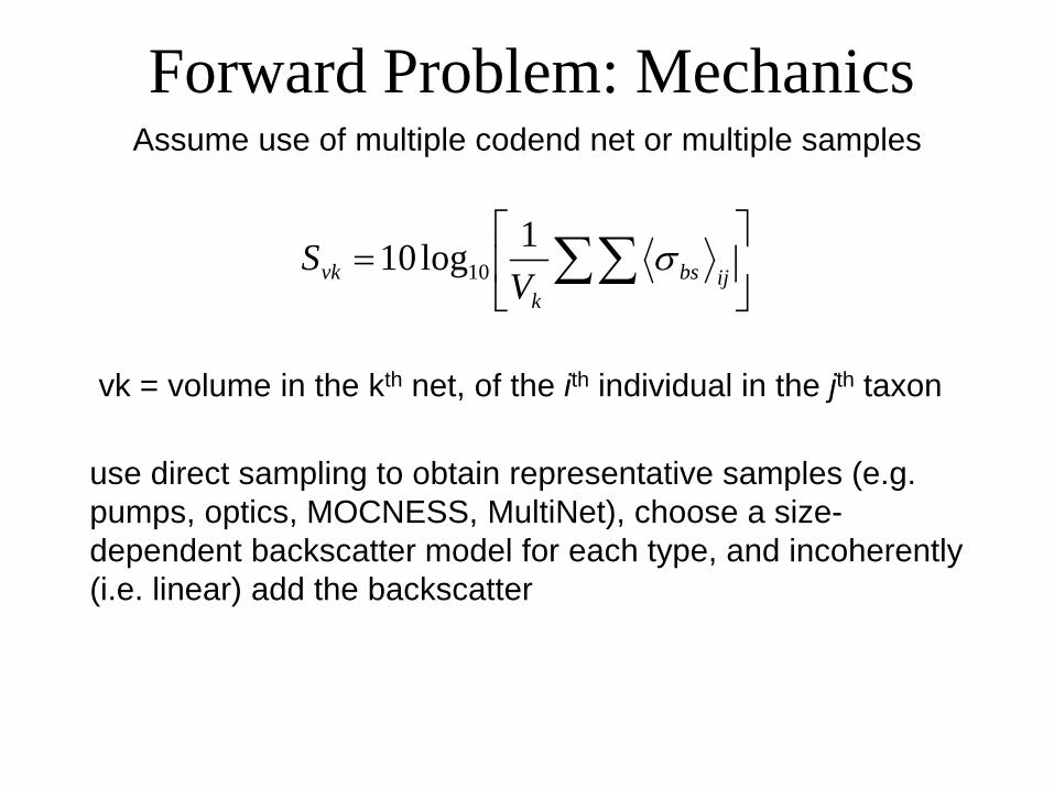
Forward Problem: Mechanics

vk = volume in the kth net, of the ith individual in the jth taxon

= ∑∑ ijbs

kvk V

S σ1log10 10

use direct sampling to obtain representative samples (e.g. pumps, optics, MOCNESS, MultiNet), choose a size-dependent backscatter model for each type, and incoherently (i.e. linear) add the backscatter

Assume use of multiple codend net or multiple samples

Forward Problem: Example

n=58, r2=0.43, p<1e-7

Lawson et al. 2004 Predicted

Obs

erve

d obs > pred

Average deviation from 1:1 = 6.8 dB

euphausiids, copepods, pteropods, siphonopohores

Why the mismatch?

The ‘Simple’ Inverse Approach

n = sv ÷ < σbs>

number of organisms = total backscatter ÷ representative acoustic size

• empirical measurement

• fish and zooplankton acoustics (more in zoop)

• rarely compared to independent data

Inverse Algorithm Concept

If you have:

- backscatter measurements at multiple frequencies

- frequency-dependent backscatter

- size-dependent backscatter models

Then you can:

- partition total backscatter by representative acoustic sizes to get size-dependent abundance estimates

Acoustic Data Processing Options

Inverse Approach

Backscatter Model

Horne & Jech 1998

Multifrequency Data

Inverse Approach Evolution Step Two:

Differences in echo levels at 2 frequencies could be used to estimate biomass within a size range (McNaught 1969)

Step Three:

Holliday (1977) published a formal mathematical method for estimation of size-based abundance estimates

Step Four:

Improved solutions for multiple-frequencies applied to small, swimbladdered fish (Johnson 1977)

Depends on Characteristic Backscatter

McNaught 1969

F(kHz)

80

120

200

500

1000

maximal backscatter at different frequencies depending on diameter

Diameter (mm)

Inverse Approach Assumptions

1. Organisms are randomly distributed within insonified region

2. Large number of scatterers in region

3. If fish, then no multiple backscatter

Greenlaw & Johnson 1983

Additional Assumptions 1. a validated backscatter model exists

2. multiple scattering effects are negligible

3. shadowing effects are negligible

4. dependence of reflectivity on other parameters is known (e.g. temperature, salinity)

5. measurements are stationary and power can be estimated

6. frequencies must span transition from Rayleigh to geometric scattering for all organisms

Holliday & Pieper 1983

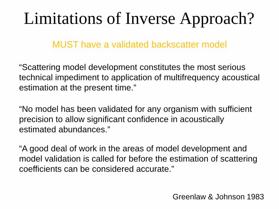
Limitations of Inverse Approach?

Greenlaw & Johnson 1983

“Scattering model development constitutes the most serious technical impediment to application of multifrequency acoustical estimation at the present time.”

“No model has been validated for any organism with sufficient precision to allow significant confidence in acoustically estimated abundances.”

“A good deal of work in the areas of model development and model validation is called for before the estimation of scattering coefficients can be considered accurate.”

MUST have a validated backscatter model

Current Backscatter Model Perception

Lavery et al. 2007

frequency

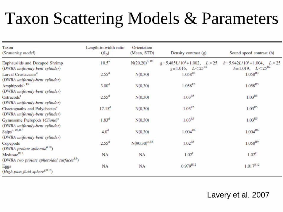
Taxon Scattering Models & Parameters

Lavery et al. 2007

Inverse Linear Addition

∑=

=N

jjijv ns

i1σ

Total backscatter (svi) of a group is the sum of backscatter from individual (si) in length class j times the number of organisms (n) in length class j over N length classes

At any frequency i

sv is a linear function of σbs

Inverse Approach Algorithm

3332321313

3232221212

3132121111

nnnsnnns

nnns

σσσσσσσσσ

++=++=++=

Measured backscatter at three frequencies (S1, S2, S3) for three length classes:

Solving equations for vector n provides abundance estimates in each length class

under, even, over determined problems

Inverse Approach Algorithm

0)(1

2 =

−∑

=

M

ivv

jii

ssn∂∂

Criterion for ‘solving’ N equations:

Minimize the sum of the squared deviations between calculated sv and measured backscatter sv for M frequencies

NNLS Non-negative least-squares (Lawson and Hanson 1974) constraint: no negative abundances in any length class j

Inverse Algorithm Alternatives

1. Least Squares

2. Regularization Methods: similar to least squares but smoothed result, multiple solutions possible

3. Backus-Gilbert Inversion: similar to regularization but parameter is bounded

Potential Measurement Error Sources 1. Random Error – assumes stationarity, minimize variance

(70 pings for 1 dB of uncertainty ≈ 12%)

2. Bias Error – noise, signal to noise ratio (min. 12 dB will increase variance by 25%)

3. Validity Error – adequate sample numbers for model averages (defines resolution of the data)

Greenlaw & Johnson 1983

User Decisions 1. Measurement frequencies

2. Size classes

3. Spatial Coverage and Resolution of Samples (beamwidth and directivity)

4. Analytic algorithm

5. Backscatter Model

Decisions based on assumed sizes and distribution of targeted population

Inverse Approach Application

Frequency (kHz)0 1 2

0.00

0.02

0.04

0.06

0.08

0.10

0.12

112 mm

36 mm

Red

uced

Sca

tterin

g Le

ngth

Threadfin shad

-use ‘acoustic volume reverberation’ (i.e. resonant backscatter)

-must span Rayleigh to geometric scattering (Holliday& Pieper 1995)

Can technique be used with geometric scattering

frequencies?

Threadfin shad (Dorosoma petenense)

How to Validate Technique? Can’t:

- demonstrate mathematical accuracy of acoustic abundance estimates on wild populations

Can:

- use simulated populations with known backscatter characteristics to quantify accuracy of abundance estimates

Inverse Simulations

How do acoustic carrier frequency and length class choices influence accuracy of length-based abundance estimates?

Tools available:

- 5 geometric backscattering frequencies 38, 70, 120, 200, 420 kHz

- representative length frequency distributions from net hauls

- KRM backscatter model

Threadfin Shad Populations

40 60 80 100 1200

10

20

30

40

Freq

uenc

y

Length (mm)

40 60 80 100 1200

10

20

30

40

40 60 80 100 1200

10

20

30

40

40 60 80 100 1200

10

20

30

40

a b

c d

Purse Seine Catches

Simulated

Per Capita Deviance Measures

nnn

total−

=∆ˆ

∑=

−=∆

N

j j

jjwithin n

nn

1

ˆPopulation Estimate Index Within Length-class Index

If ‘perfect’ estimate then index values = 0

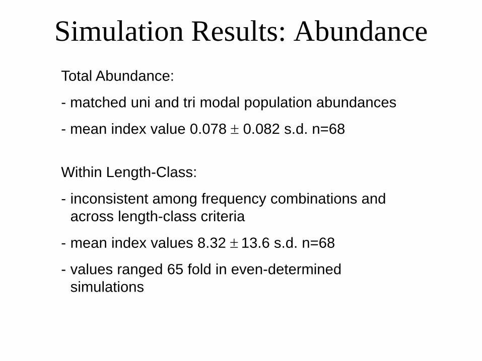
Simulation Results: Abundance Total Abundance:

- matched uni and tri modal population abundances

- mean index value 0.078 ± 0.082 s.d. n=68

Within Length-Class:

- inconsistent among frequency combinations and across length-class criteria

- mean index values 8.32 ± 13.6 s.d. n=68

- values ranged 65 fold in even-determined simulations

Simulation Results: Frequency Total Abundance:

- ‘best’ estimates all contained 70, 200 kHz

- equal interval centered on mean(s)

Within Length-Class:

- ‘best’ estimates all contained 38, 70, 120 kHz

- ‘best’ size class criterion was equal interval across range (compared to means, node and null values)

Frequency & Length Dependent Backscatter

0.00

0.04

0.08

L/λ

Red

uced

Sca

tterin

g Le

ngth

0.00

0.04

0.08

0.00

0.04

0.08

0.00

0.04

0.08

0 10 20 300.00

0.04

0.08

a

b

c

d

e

Length Range

36 – 112 mm 38

70

120

200

420

Frequency (kHz)

Multiple Frequency Choice

0 10 20 300.00

0.02

0.04

0.06

0.08

L/λ

38 kHz70 kHz120 kHz

Sca

tterin

gLe

ngth

Red

uced

0 10 20 300.00

0.02

0.04

0.06

0.0838 kHz70 kHz120 kHz200 kHz420 kHz

L/λS c

a tt e

r ing

L en g

t hR

e du c

e d

3 Frequency 5 Frequency

non-unique amplitude – L/λ combinations

Reference Backscatter Values - ‘best’ results occurred when L/λ values

encompassed full amplitude range, minimized overlap among reference scattering points, and maximized number of features defined

Feature = peak or valley on the backscatter curve

- three points are needed to define a feature

Threadfin Shad Backscatter Response

0

5

10

15

20

25

90

70

80

100

0.02

0.04

0.06

0.08

0.10R

educ

ed S

catte

ring

Leng

th

θL/λ

head down

head up

Reduced Scattering Length

0.0004 0.088

60

modeled length 75 mm

What about behavioral

effects?