formulation of disperse systems (science and technology) || formulation of liquid/liquid dispersions...

161

10Formulation of Liquid/Liquid Dispersions (Emulsions)

10.1Introduction

Emulsions are a class of disperse systems consisting of two immiscible liquids[1–3], whereby the liquid droplets (the disperse phase) are dispersed in a liquidmedium (the continuous phase). Several classes of emulsion may be distinguished,namely Oil-in-Water (O/W), Water-in-Oil (W/O), and Oil-in-Oil (O/O). The latterclass may be exemplified by an emulsion consisting of a polar oil (e.g., propyleneglycol) dispersed in a nonpolar oil (paraffinic oil), and vice versa. In order to dispersetwo immiscible liquids a third component is needed, namely the emulsifier. Thechoice of the emulsifier is crucial in the formation of an emulsion and its long-termstability [1–3].

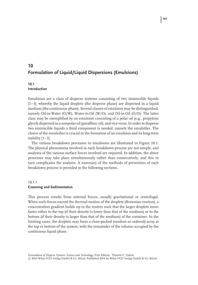
The various breakdown processes in emulsions are illustrated in Figure 10.1.The physical phenomena involved in each breakdown process are not simple, andanalyses of the various surface forces involved are required. In addition, the aboveprocesses may take place simultaneously rather than consecutively, and this inturn complicates the analysis. A summary of the methods of prevention of eachbreakdown process is provided in the following sections.

10.1.1Creaming and Sedimentation

This process results from external forces, usually gravitational or centrifugal.When such forces exceed the thermal motion of the droplets (Brownian motion), aconcentration gradient builds up in the system such that the larger droplets movefaster either to the top (if their density is lower than that of the medium) or to thebottom (if their density is larger than that of the medium) of the container. In thelimiting cases, the droplets may form a close-packed (random or ordered) array atthe top or bottom of the system, with the remainder of the volume occupied by thecontinuous liquid phase.

Formulation of Disperse Systems: Science and Technology, First Edition. Tharwat F. Tadros.c© 2014 Wiley-VCH Verlag GmbH & Co. KGaA. Published 2014 by Wiley-VCH Verlag GmbH & Co. KGaA.

162 10 Formulation of Liquid/Liquid Dispersions (Emulsions)

Creaming

Phase

inversion

Sedimentation

Coalescence

Flocculation

Ostwaldripening

Figure 10.1 Schematic representation of the various breakdown processes in emulsions.

10.1.2Flocculation

This process refers to aggregation of the droplets (without any change in primarydroplet size) into larger units. It is the result of the van der Waals attractionsthat are universal with all disperse systems. Flocculation occurs when thereis insufficient repulsion to keep the droplets apart at distances where the vander Waals attractions are weak. Flocculation may be either ‘‘strong’’ or ‘‘weak,’’depending on the magnitude of the attractive energy involved.

10.1.3Ostwald Ripening (Disproportionation)

This results from the finite solubility of the liquid phases. Liquids which are referredto as being immiscible often have mutual solubilities which are not negligible. Inthe case of emulsions, which are usually polydisperse, the smaller droplets willhave a greater solubility compared to the larger droplets (due to curvature effects).With time, however, the smaller droplets will disappear and their molecules willdiffuse to the bulk and become deposited on the larger droplets. With time, thedroplet size distribution will shift to a larger value.

10.2 Industrial Applications of Emulsions 163

10.1.4Coalescence

This refers to the process of thinning and disruption of the liquid film betweenthe droplets, with the result that two or more droplets fuse into a larger droplet.The limiting case for coalescence is the complete separation of the emulsion intotwo distinct liquid phases. The driving force for coalescence is the surface or filmfluctuations; this results in a close approach of the droplets whereby the van derWaals forces are strong and prevent their separation.

10.1.5Phase Inversion

This refers to the process when an exchange occurs between the disperse phaseand the medium. For example, an O/W emulsion may, with time or change ofconditions, invert to a W/O emulsion. In many cases phase inversion passesthrough a transition state whereby multiple emulsions are produced.

10.2Industrial Applications of Emulsions

Several industrial systems involve emulsions, of which the following are wor-thy of mention. Food emulsions include mayonnaise, salad creams, deserts,and beverages, while personal care and cosmetics emulsions include handcreams, lotions, hair sprays, and sunscreens. Agrochemical emulsions includeself-emulsifiable oils that produce emulsions on dilution with water, emulsionconcentrates with water as the continuous phase, and crop oil sprays. Pharma-ceutical emulsions include anaesthetics (O/W emulsions), lipid emulsions, anddouble and multiple emulsions, while paints may involve emulsions of alkydresins and latex. Some dry-cleaning formulations may contain water dropletsemulsified in the dry cleaning oil that is necessary to remove soils and clays,while bitumen emulsions are prepared stable in their containers but coalesceto form a uniform film of bitumen when applied with road chippings. Inthe oil industry, many crude oils (e.g., North sea oil) contain water dropletsthat must be removed by coalescence followed by separation. In oil slick dis-persion, the oil spilled from tankers must be emulsified and then separated,while the emulsification of waste oils is an important process for pollutioncontrol.

The above-described importance of emulsion in many industries justifies theextensive research that has been carried out to understand the origins of emulsioninstability and methods to prevent their breakdown. Unfortunately, fundamentalresearch with emulsions is not easy, as model systems (e.g., with monodispersedroplets) are difficult to produce. In many cases, theories on emulsion stability arenot exact and semi-empirical approaches must be used.


10.3Physical Chemistry of Emulsion Systems

10.3.1The Interface (Gibbs Dividing Line)

An interface between two bulk phases, for example liquid and air (or liquid/vapour)or two immiscible liquids (oil/water) may be defined provided that a dividing lineis introduced (Figure 10.2). The interfacial region is not a layer that is one moleculethick; rather, it is a region with thickness 𝛿 and properties which differ from thoseof the two bulk phases 𝛼 and 𝛽.

Using the Gibbs model, it is possible to obtain a definition of the surface orinterfacial tension 𝛾 . The surface free energy dGσ comprises three components: (i)an entropy term S𝜎dT ; (ii) an interfacial energy term Ad𝛾 , and (iii) a compositionterm Σ nid𝜇i (where ni is the number of moles of component i with chemicalpotential 𝜇i). The Gibbs–Duhem equation is,

dG𝜎 = −S𝜎dT + Ad𝛾 +∑

nid𝜇i (10.1)

At constant temperature and composition,

dG𝜎 = Ad𝛾

𝛾 =(∂G𝜎

∂A

)T ,ni

(10.2)

For a stable interface 𝛾 is positive; that is, if the interfacial area increases G𝜎

increases. Note that 𝛾 is energy per unit area (mJ m−2), which is dimensionallyequivalent to force per unit length (mN m−1), the unit usually used to define surfaceor interfacial tension.

For a curved interface the effect of the radius of curvature should be considered.Fortunately, 𝛾 for a curved interface is estimated to be very close to that of a planersurface, unless the droplets are very small (<10 nm). Curved interfaces producesome other important physical phenomena which affect emulsion properties, suchas the Laplace pressure Δp, which is determined by the radii of curvature of thedroplets,

Δp = 𝛾

(1r1

+ 1r2

)(10.3)

where r1 and r2 are the two principal radii of curvature.

Uniformthermodynamic

properties

Uniformthermodynamic

properties

Mathematical dividing

Plane Zσ

(Gibbs dividing line)

Figure 10.2 The Gibbs dividing line.

10.3 Physical Chemistry of Emulsion Systems 165

For a perfectly spherical droplet r1 = r2 = r and

Δp = 2𝛾r

(10.4)

For a hydrocarbon droplet with radius 100 nm, and 𝛾 = 50 mN m−1, Δp is approx-imately 106 Pa (10 atm).

10.3.2Thermodynamics of Emulsion Formation and Breakdown

Consider a system in which an oil is represented by a large drop 2 of area A1

immersed in a liquid 2, which is now subdivided into a large number of smallerdroplets with total area A2 (A2 ≫ A1), as shown in Figure 10.3. The interfacialtension 𝛾12 is the same for the large and smaller droplets as the latter are generallyin the region of 0.1 to few micrometres.

The change in free energy in going from state I to state II is made from twocontributions: (i) a surface energy term (that is positive) that is equal to ΔA 𝛾12

(where ΔA=A2 −A1); and (ii) an entropy of dispersions term which is also positive(since the production of a large number of droplets is accompanied by an increasein configurational entropy) which is equal to T ΔSconf.

From the Second law of Thermodynamics,

ΔGform = ΔA𝛾12 − TΔSconf (10.5)

In most cases ΔA𝛾12 ≫T ΔSconf, which means that ΔGform is positive; that is, theformation of emulsions is nonspontaneous and the system is thermodynamicallyunstable. In the absence of any stabilisation mechanism, the emulsion will breakby flocculation, coalescence, Ostwald ripening, or a combination of all theseprocesses. This is illustrated in Figure 10.4, which shows several pathways foremulsion breakdown processes.

In the presence of a stabiliser (surfactant and/or polymer), an energy barrier iscreated between the droplets, and therefore the reversal from state II to state Ibecomes noncontinuous as a result of the presence of these energy barriers; this isillustrated in Figure 10.5. In the presence of the above energy barriers, the systembecomes kinetically stable.

I II

12

2

1Formation

Breakdown

(Flocc + coal)

Figure 10.3 Schematic representation of emulsion formation and breakdown.


II or IV I or III

GII

GlV

GIII

GI

Figure 10.4 Free energy path in emulsion breakdown. The solid line indicates flocculation+ coalescence; the dashed line indicates flocculation + coalescence + sedimentation; the dot-ted line indicates flocculation + coalescence + sedimentation + Ostwald ripening.

GII

GV

GI

ΔGcoal

ΔGcoala

ΔGflocca

ΔGflocc ΔGbreak

II IV

Figure 10.5 Schematic representation of free energy path for breakdown (flocculation andcoalescence) for systems containing an energy barrier.

10.3.3Interaction Energies (Forces) between Emulsion Droplets and Their Combinations

Generally speaking, there are three main interaction energies (forces) betweenemulsion droplets and these are discussed below.

10.3.3.1 van der Waals AttractionsThe van der Waals attractions between atoms or molecules are of three differenttypes: dipole–dipole (Keesom), dipole-induced dipole (Debye), and dispersion(London) interactions. The Keesom and Debye attraction forces are vectors, and


although dipole–dipole or dipole-induced dipole attractions are large they tend tocancel due to the different orientations of the dipoles. Thus, the most importantare the London dispersion interactions which arise from charge fluctuations. Withatoms or molecules consisting of a nucleus and electrons that are continuouslyrotating around the nucleus, a temporary dipole is created as a result of chargefluctuations. This temporary dipole induces another dipole in the adjacent atomor molecule. The interaction energy between two atoms or molecules Ga is shortrange and is inversely proportional to the sixth power of the separation distance rbetween the atoms or molecules,

Ga = − 𝛽

r6(10.6)

where 𝛽 is the London dispersion constant that is determined by the polarisabilityof the atom or molecule.

Hamaker [4] suggested that the London dispersion interactions between atomsor molecules in macroscopic bodies (such as emulsion droplets) can be added,resulting in strong van der Waals attractions, particularly at close distances ofseparation between the droplets. For two droplets with equal radii, R, at a separationdistance h, the van der Waals attraction GA is given by the following equation (dueto Hamaker):

GA = −𝐴𝑅

12h(10.7)

where A is the effective Hamaker constant,

A =(

A1∕211 − A1∕2

22

)2(10.8)

where A11 and A22 are the Hamaker constants of the droplets and dispersionmedium, respectively.

The Hamaker constant of any material depends on the number of atoms ormolecules per unit volume q and the London dispersion constant 𝛽,

A = 𝜋2q2𝛽 (10.9)

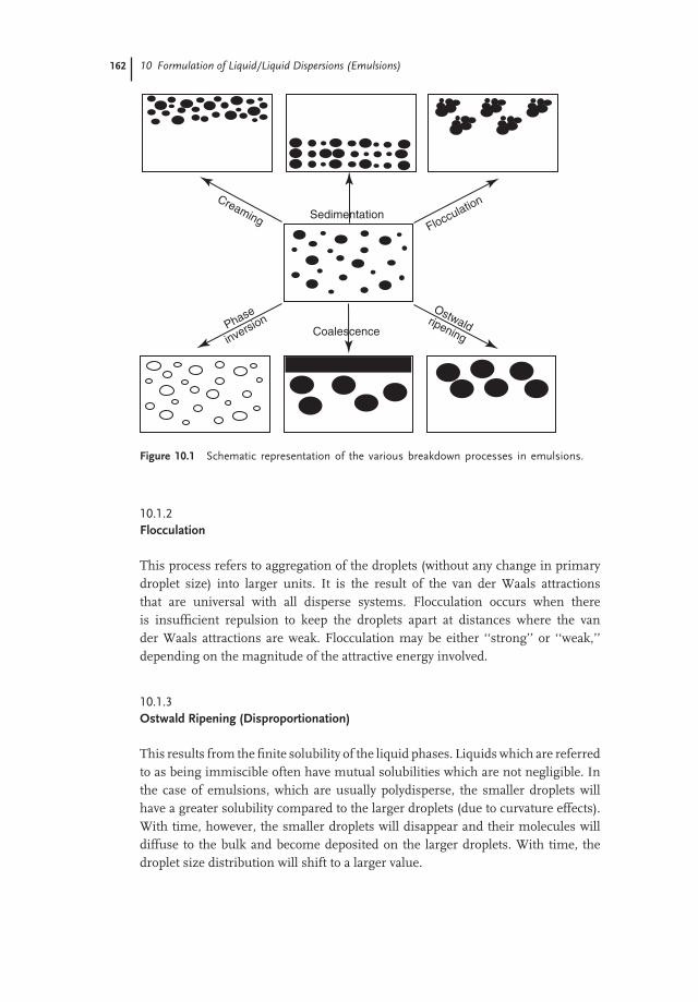
GA increases very rapidly with decrease of h (at close approach), and this isillustrated in Figure 10.6, which shows the van der Waals energy–distance curvefor two emulsion droplets with separation distance h.

In the absence of any repulsion, flocculation is very fast and produces largeclusters. In order to counteract the van der Waals attractions, it is necessaryto create a repulsive force. Two main types of repulsion can be distinguished,depending on the nature of the emulsifier used, namely electrostatic (due to thecreation of double layers) and steric (due to the presence of adsorbed surfactant orpolymer layers).

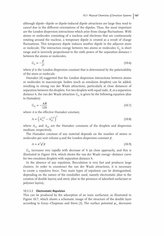
10.3.3.2 Electrostatic RepulsionThis can be produced by the adsorption of an ionic surfactant, as illustrated inFigure 10.7, which shows a schematic image of the structure of the double layeraccording to Gouy–Chapman and Stern [3]. The surface potential 𝜓o decreases


h

GA

Bornrepulsion

Figure 10.6 Variation of the van der Waals attraction energy with separation distance.

−

−

−

−

−

Stern plane X

+

+

+

+

+

+

+

+

+

+

+

+

−−

−−

−

𝛹o 𝛹d

𝜎d𝜎o

𝜎o = 𝜎s + 𝜎d

𝜎s = Charge due to

Specifically adsorbedcounter ions

𝜎s

Figure 10.7 Schematic representation of double layers produced by adsorption of an ionicsurfactant.

linearly to 𝜓d (Stern or zeta-potential) and then exponentially with increase of thedistance x. The double layer extension depends on electrolyte concentration andvalency (the lower the electrolyte concentration and the lower the valency, the moreextended the double layer is).

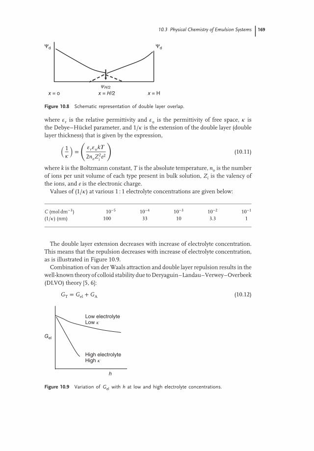
When charged colloidal particles in a dispersion approach each other such thatthe double layer begins to overlap (when particle separation becomes less thantwice the double layer extension), then repulsion will occur. The individual doublelayers can no longer develop unrestrictedly, as the limited space does not allowcomplete potential decay [3]. This is illustrated in Figure 10.8 for two flat plates,and shows clearly shows that when the separation distance h between the emulsiondroplets become less than twice the doubly layer extension, the potential at the midplane between the surfaces is not equal to zero (which would be the case if h weremore than twice the double layer extension) plates.

The repulsive interaction Gel is given by the following expression,

Gel = 2𝜋𝑅𝜀r𝜀o𝜓2o ln[1 + exp(−𝜅ℎ)] (10.10)


𝜓H/2

x = o x = H/2 x = H

Ψd Ψd

Figure 10.8 Schematic representation of double layer overlap.

where 𝜀r is the relative permittivity and 𝜀o is the permittivity of free space, 𝜅 isthe Debye–Huckel parameter, and 1/𝜅 is the extension of the double layer (doublelayer thickness) that is given by the expression,( 1

𝜅

)=

(𝜀r𝜀o𝑘𝑇

2noZ2ie2

)(10.11)

where k is the Boltzmann constant, T is the absolute temperature, no is the numberof ions per unit volume of each type present in bulk solution, Zi is the valency ofthe ions, and e is the electronic charge.

Values of (1/𝜅) at various 1 : 1 electrolyte concentrations are given below:

C (mol dm−3) 10−5 10−4 10−3 10−2 10−1

(1/𝜅) (nm) 100 33 10 3.3 1

The double layer extension decreases with increase of electrolyte concentration.This means that the repulsion decreases with increase of electrolyte concentration,as is illustrated in Figure 10.9.

Combination of van der Waals attraction and double layer repulsion results in thewell-known theory of colloid stability due to Deryaguin–Landau–Verwey–Overbeek(DLVO) theory [5, 6]:

GT = Gel + GA (10.12)

Low electrolyteLow 𝜅

High electrolyteHigh 𝜅

Gel

h

Figure 10.9 Variation of Gel with h at low and high electrolyte concentrations.


G

Gmax

GeGT

GA Gsec

h

Gprimary

Figure 10.10 Total energy–distance curve according to DLVO theory.

A schematic representation of the force (energy)–distance curve, according toDLVO theory, is shown in Figure 10.10.

The above presentation is for a system at low electrolyte concentration. At largeh, attraction prevails resulting in a shallow minimum (Gsec) on the order of fewkT units. At very short h, VA ≫Gel, resulting in a deep primary minimum (severalhundred kT), while at intermediate h, Gel >GA, resulting in a maximum (energybarrier) whose height depends on 𝜓o (or 𝜁 ) and electrolyte concentration andvalency; the energy maximum is usually kept at >25 kT. The energy maximum pre-vents close approach of the droplets, and flocculation into the primary minimumis also prevented. The higher the value of 𝜓o and the lower the electrolyte concen-tration and valency, the higher the energy maximum. At intermediate electrolyteconcentrations, weak flocculation into the secondary minimum may occur.

10.3.3.3 Steric RepulsionThis is produced by using nonionic surfactants or polymers, for example alco-hol ethoxylates, or A-B-A block copolymers PEO-PPO-PEO (where PEO refersto polyethylene oxide and PPO refers to polypropylene oxide), as illustrated inFigure 10.11.

Alkyl chain

PEO

PPO

PEO

Figure 10.11 Schematic representation of adsorbed layers.


The ‘‘thick’’ hydrophilic chains (PEO in water) produce repulsion as a result oftwo main effects [7]:

• Unfavourable mixing of the PEO chains: When these are in good solventconditions (moderate electrolyte and low temperatures), this is referred to as theosmotic or mixing free energy of interaction, that is given by the expression,

Gmix

𝑘𝑇=(

4𝜋V1

)𝜑2

2Nav

(12− 𝜒

)(𝛿 − h

2

)2 (3R + 2𝛿 + h

2

)(10.13)

where V1 is the molar volume of the solvent, 𝜑2 is the volume fraction ofthe polymer chain with a thickness 𝛿, and 𝜒 is the Flory–Huggins interactionparameter. When 𝜒 < 0.5, Gmix is positive and the interaction is repulsive, butwhen 𝜒 > 0.5, Gmix is negative and the interaction is attractive. When 𝜒 = 0.5 andGmix = 0, this is referred to as the θ-condition.

• Entropic, volume restriction or elastic interaction, Gel: This results from the lossin configurational entropy of the chains on significant overlap. Entropy loss isunfavourable and, therefore, Gel is always positive. A combination of Gmix, Gel

with GA gives the total energy of interaction GT (theory of steric stabilisation),

GT = Gmix + Gel + GA (10.14)

A schematic representation of the variation of Gmix, Gel and GA with h is givenin Figure 10.12. Gmix increases very sharply with a decrease of h when the latterbecomes less than 2𝛿, while Gel increases very sharply with a decrease of h whenthe latter becomes smaller than 𝛿. GT increases very sharply with a decrease of hwhen the latter becomes less than 2𝛿.

Figure 10.12 shows that there is only one minimum (Gmin) whose depth dependson R, 𝛿 and A. At a given droplet size and Hamaker constant, the larger the adsorbedlayer thickness, the smaller the depth of the minimum. If Gmin is made sufficientlysmall (large 𝛿 and small R), then thermodynamic stability may be approaching.

G

Gel

Gmix

Gmin

h

GT

GA

𝛿2𝛿

Figure 10.12 Schematic representation of the energy–distance curve for a stericallystabilised emulsion.


Increasing 𝛿/R

Gmin

Gr

h

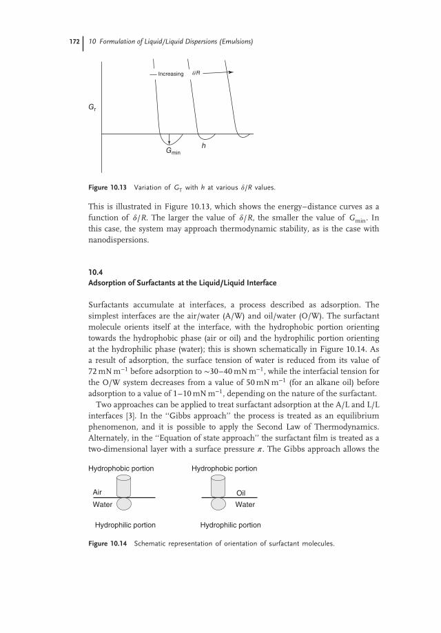
Figure 10.13 Variation of GT with h at various 𝛿/R values.

This is illustrated in Figure 10.13, which shows the energy–distance curves as afunction of 𝛿/R. The larger the value of 𝛿/R, the smaller the value of Gmin. Inthis case, the system may approach thermodynamic stability, as is the case withnanodispersions.

10.4Adsorption of Surfactants at the Liquid/Liquid Interface

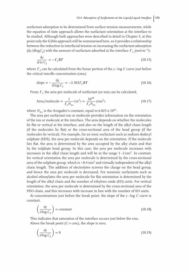
Surfactants accumulate at interfaces, a process described as adsorption. Thesimplest interfaces are the air/water (A/W) and oil/water (O/W). The surfactantmolecule orients itself at the interface, with the hydrophobic portion orientingtowards the hydrophobic phase (air or oil) and the hydrophilic portion orientingat the hydrophilic phase (water); this is shown schematically in Figure 10.14. Asa result of adsorption, the surface tension of water is reduced from its value of72 mN m−1 before adsorption to ∼30–40 mN m−1, while the interfacial tension forthe O/W system decreases from a value of 50 mN m−1 (for an alkane oil) beforeadsorption to a value of 1–10 mN m−1, depending on the nature of the surfactant.

Two approaches can be applied to treat surfactant adsorption at the A/L and L/Linterfaces [3]. In the ‘‘Gibbs approach’’ the process is treated as an equilibriumphenomenon, and it is possible to apply the Second Law of Thermodynamics.Alternately, in the ‘‘Equation of state approach’’ the surfactant film is treated as atwo-dimensional layer with a surface pressure 𝜋. The Gibbs approach allows the

Water

Oil

Hydrophobic portion

Hydrophilic portion Hydrophilic portion

Hydrophobic portion

Air

Water

Figure 10.14 Schematic representation of orientation of surfactant molecules.

10.4 Adsorption of Surfactants at the Liquid/Liquid Interface 173

surfactant adsorption to be determined from surface tension measurements, whilethe equation of state approach allows the surfactant orientation at the interface tobe studied. Although both approaches were described in detail in Chapter 5, at thispoint only the Gibbs approach will be summarised here, as it provides a relationshipbetween the reduction in interfacial tension on increasing the surfactant adsorption(d𝛾/dlogC2) with the amount of surfactant adsorbed at the interface 𝛤 2 (mol m−2):

d𝛾d ln C2

= −𝛤2𝑅𝑇 (10.15)

where 𝛤 2 can be calculated from the linear portion of the 𝛾 –log C curve just beforethe critical micelle concentration (cmc):

slope = − d𝛾d log C2

= −2.303𝛤2𝑅𝑇 (10.16)

From 𝛤 2 the area per molecule of surfactant (or ion) can be calculated,

Area∕molecule = 1𝛤2NAv

(m2) = 1018

𝛤2NAv(nm2) (10.17)

where NAv is the Avogadro’s constant, equal to 6.023× 1023.The area per surfactant ion or molecule provides information on the orientation

of the ion or molecule at the interface. The area depends on whether the moleculeslie flat or vertical at the interface, and also on the length of the alkyl chain length(if the molecules lie flat) or the cross-sectional area of the head group (if themolecules lie vertical). For example, for an ionic surfactant such as sodium dodecylsulphate (SDS), the area per molecule depends on the orientation. If the moleculelies flat, the area is determined by the area occupied by the alky chain and thatby the sulphate head group. In this case, the area per molecule increases withincreases in the alkyl chain length and will be in the range 1–2 nm2. In contrast,for vertical orientation the area per molecule is determined by the cross-sectionalarea of the sulphate group, which is ∼0.4 nm2 and virtually independent of the alkylchain length. The addition of electrolytes screens the charge on the head group,and hence the area per molecule is decreased. For nonionic surfactants such asalcohol ethoxylates the area per molecule for flat orientation is determined by thelength of the alkyl chain and the number of ethylene oxide (EO) units. For verticalorientation, the area per molecule is determined by the cross-sectional area of thePEO chain, and this increases with increase in line with the number of EO units.

At concentrations just before the break point, the slope of the 𝛾 –log C curve isconstant,(

∂𝛾∂ log C2

)= constant (10.18)

This indicates that saturation of the interface occurs just below the cmc.Above the break point (C > cmc), the slope is zero,(

∂𝛾∂ log C2

)= 0 (10.19)


or

𝛾 = constant x log C2 (10.20)

Since 𝛾 remains constant above the cmc, then C2 or a2 of the monomer mustremain constant.

The addition of surfactant molecules above the cmc must result in an associationto form micelles which have low activity, and hence a2 will remain virtually constant.

The hydrophilic head group of the surfactant molecule can also affect itsadsorption. Such head groups can be unionised, for example alcohol or PEO(weakly ionised such as COOH, or strongly ionised such as sulphates –O–SO3

−,sulphonates -SO3

− or ammonium salts -N+(CH3)3-). The adsorption of the differentsurfactants at the A/W and O/W interfaces depends on the nature of the head group.With nonionic surfactants, repulsion between the head groups is less than withionic head groups and adsorption occurs from dilute solutions; in this case the cmcis low, typically 10−5 to 10−4 mol dm−3. Nonionic surfactants with medium PEOform closely packed layers at C < cmc, when adsorption will be slightly affected bythe moderate addition of electrolytes or by a change in the pH. Nonionic surfactantadsorption is relatively simple and can be described using the Gibbs adsorptionequation.

With ionic surfactants, adsorption is more complicated depending on the repul-sion between the head groups and the addition of indifferent electrolytes. TheGibbs adsorption equation must be solved to take into account the adsorption ofthe counterions and any indifferent electrolyte ions.

For a strong surfactant electrolyte such as R–O–SO3− Na+ (R− Na+):

𝛤2 = − 12𝑅𝑇

(∂𝛾

∂ ln a±

)(10.21)

The factor of 2 in Equation (10.21) arises because both surfactant ion andcounterion must be adsorbed to maintain neutrality. (∂𝛾/dln a±) is twice as largefor an unionised surfactant molecule.

For a nonadsorbed electrolyte such as NaCl, any increase in Na+ R− concentrationproduces a negligible increase in Na+ concentration (d𝜇Na

+ is negligible and d𝜇Cl−

is also negligible.

𝛤2 = − 1𝑅𝑇

(∂𝛾

∂ ln CNaR

)(10.22)

which is identical to the case of nonionics.The above analysis shows that many ionic surfactants may behave like nonionics

in the presence of a large concentration of an indifferent electrolyte such as NaCl.

10.4.1Mechanism of Emulsification

As mentioned previously, the requirements to prepare an emulsion include oil,water, surfactant, and energy, and this can be considered from the energy requiredto expand the interface, ΔA𝛾 (where ΔA is the increase in interfacial area when the


bulk oil with area A1 produces a large number of droplets with area A2; A2 ≫A1,and 𝛾 is the interfacial tension). As 𝛾 is positive, the energy needed to expand theinterface is large and positive, and cannot be compensated by the small entropy ofdispersion TΔS (which is also positive); moreover, the total free energy of formationof an emulsion,ΔG, given by Equation (10.5), is positive. Thus, emulsion formationis nonspontaneous and energy is required to produce the droplets.

The formation of large droplets (a few micrometres in size), as is the case formacroemulsions, is fairly easy and high-speed stirrers such as the UltraTurrax orSilverson mixer are sufficient to produce such emulsions. In contrast, the formationof small drops (submicron, as is the case with nanoemulsions) is difficult and thisrequires a large amount of surfactant and/or energy. The high energy requiredfor formation of nanoemulsions can be understood from a consideration of theLaplace pressure Δp (the difference in pressure between the inside and outside ofthe droplet), as given by Equations (10.3) and (10.4).

In order to break up a drop into smaller units it must be strongly deformed,and this deformation increases Δp. Surfactants play major roles in the formationof emulsions [8]; by lowering the interfacial tension Δp is reduced, and hencethe stress needed to break up a drop is reduced. Surfactants also prevent thecoalescence of newly formed drops.

To describe emulsion formation two main factors must be considered, namelyhydrodynamics and interfacial science. In hydrodynamics, consideration must begiven to the type of flow, whether laminar or turbulent, and this depends on theReynolds number (as will be discussed later).

To assess emulsion formation, the normal approach is to measures the dropletsize distribution using, for example laser diffraction techniques. A useful averagediameter d is,

d𝑛𝑚 =(

Sm

Sn

)1∕(n−m)

(10.23)

In most cases d32 (the volume/surface average or Sauter mean) is used, whilethe width of the size distribution can be given as the variation coefficient cm . Thelatter is the standard deviation of the distribution weighted with dm divided by thecorresponding average d. Generally C2 will be used which corresponds to d32.

An alternative way to describe the emulsion quality is to use the specific surfacearea A (the surface area of all emulsion droplets per unit volume of emulsion),

A = 𝜋s2 = 6𝜙d32

(10.24)

10.4.2Methods of Emulsification

Several procedures may be applied for emulsion preparation, ranging from simplepipe flow (low agitation energy, L), static mixers and general stirrers (low to mediumenergy, L-M), high-speed mixers such as the UltraTurrax (M), colloid mills and high-pressure homogenisers (high energy, H), ultrasound generators (M-H). In addition,


the method of preparation can be either continuous or batch-wise: typically, pipeflow and static mixers are continuous; stirrers and UltraTurrax are batchwise andcontinuous; colloid mill and high-pressure homogenisers are continuous; andultrasound is both batchwise and continuous.

In all methods there is liquid flow with unbounded and strongly confined flow.In the unbounded flow, any droplets are surrounded by a large amount of flowingliquid (the confining walls of the apparatus are far away from most droplets), whilethe forces can be either frictional (mostly viscous) or inertial. Viscous forces causeshear stresses to act on the interface between the droplets and the continuous phase(primarily in the direction of the interface). The shear stresses can be generatedby either laminar flow (LV) or turbulent flow (TV); this depends on the Reynoldsnumber Re,

Re =𝑣𝑙𝜌

𝜂(10.25)

where v is the linear liquid velocity, 𝜌 is the liquid density, 𝜂 is its viscosity, and lis a characteristic length that is given by the diameter of flow through a cylindricaltube and by twice the slit width in a narrow slit.

For laminar flow Re <∼1000, whereas for turbulent flow Re >∼2000. Thus,whether the regime is linear or turbulent depends on the scale of the apparatus,the flow rate, and the liquid viscosity [9–12].

If the turbulent eddies are much larger than the droplets they exert shear stresseson the droplets; however, if the turbulent eddies are much smaller than the dropletsthen inertial forces will cause disruption (turbulent/inertial).

In bounded flow other relationships hold; for example, if the smallest dimensionof the part of the apparatus in which the droplets are disrupted (e.g., a slit) iscomparable to the droplet size, the flow will always be laminar. A different regimeprevails, however, if the droplets are injected directly through a narrow capillaryinto the continuous phase (injection regime), namely membrane emulsification.

Within each regime, one essential variable is the intensity of the forces whichare acting; the viscous stress during laminar flow 𝜎viscous is given by,

𝜎viscous = 𝜂𝐺 (10.26)

where G is the velocity gradient.The intensity in turbulent flow is expressed by the power density 𝜀 (the amount

of energy dissipated per unit volume per unit time); for laminar flow,

𝜀 = 𝜂G2 (10.27)

The most important regimes are laminar/viscous (LV), turbulent/viscous (TV),and turbulent/inertial (TI). With water as the continuous phase the regime isalways TI, but when the viscosity of the continuous phase is higher (𝜂C = 0.1 Pa⋅s)the regime will be TV. For a still higher viscosity or a small apparatus (small l), theregime will be LV, and for very small apparatus (as is the case with most laboratoryhomogenisers) the regime is nearly always LV.

For the above regimes, a semi-quantitative theory is available that can providethe time scale and magnitude of the local stress 𝜎ext, the droplet diameter d, the


time scale of droplet deformation 𝜏def, the time scale of surfactant adsorption, 𝜏ads,and the mutual collision of droplets.

An important parameter that describes droplet deformation is the Weber numberWe (which gives the ratio of the external stress over the Laplace pressure),

We =G𝜂CR

2𝛾(10.28)

The viscosity of the oil plays an important role in the break-up of droplets; thehigher the viscosity, the longer it will take to deform a drop. The deformation time𝜏def is given by the ratio of oil viscosity to the external stress acting on the drop,

𝜏def =𝜂D

𝜎ext(10.29)

The viscosity of the continuous phase 𝜂C plays an important role in some regimes;for the TI regime 𝜂C has no effect on droplets size, but for the TV regime a largervalue of 𝜂C leads to smaller droplets, and for LV the effect is even stronger.

10.4.3Role of Surfactants in Emulsion Formation

Surfactants lower the interfacial tension 𝛾 , which in turn causes a reduction indroplet size; typically, the latter will decrease with a decrease in 𝛾 . For laminar flow,the droplet diameter is proportional to 𝛾 , but for a TI regime the droplet diameteris proportional to 𝛾3/5.

The effect of reducing 𝛾 on droplet size is illustrated in Figure 10.15, whichshows a plot of the droplet surface area A and mean drop size d32 as a function ofthe surfactant concentration m for various systems.

The amount of surfactant required to produce the smallest drop size will dependon its activity a (concentration) in the bulk which in turn determines the reductionin 𝛾 , as given by the Gibbs adsorption equation as discussed before,

−d𝛾 = 𝑅𝑇𝛤d ln a (10.30)

4

6

8

10

15

30

Nonionic surfactant

Casinate

PVA

Soy protein

𝛾 = 20 mNm−1

𝛾 = 10 mNm−1

𝛾 = 3 mNm−1

d32

/𝜇m

0

0.5

1.0

1.5

A/𝜇m−1

5 10

Figure 10.15 Variation of A and d32 with m for various surfactant systems.


4

2

0−7 −6 −4 −2 0

𝛤/mgm−2

SDS

𝛽-casein,emulsion

𝛽-casein, O/W interface

Figure 10.16 Variation of 𝛤 (mg m−2) with log Ceq (wt%). The oils are β-casein (O/Winterface), toluene, β-casein (emulsions), soybean, SDS benzene.

where R is the gas constant, T is the absolute temperature, and 𝛤 is the surfaceexcess (number of moles adsorbed per unit area of the interface).𝛤 increases with increases in surfactant concentration, and eventually reaches a

plateau value (saturation adsorption); this is illustrated in Figure 10.16 for variousemulsifiers.

The value of 𝛾 obtained depends on the nature of the oil and surfactant used; smallmolecules such as nonionic surfactants lower 𝛾 more than polymeric surfactantssuch as PVA.

Another important role of the surfactant is its effect on the interfacial dilationalmodulus 𝜀,

𝜀 = d𝛾d ln A

(10.31)

During emulsification an increase in the interfacial area A takes place and thiscauses a reduction in 𝛤 . The equilibrium is restored by the adsorption of surfactantfrom the bulk, but this takes time (shorter times occur at higher surfactant activity).Thus, 𝜀 is small whether a is small or large. Because of the lack or slowness ofequilibrium with polymeric surfactants, 𝜀 will not be the same for expansion andcompression of the interface.

In practice, surfactant mixtures are used that may have pronounced effects on𝛾 and 𝜀. Some specific surfactant mixtures produce lower 𝛾-values than either ofthe two individual components, while the presence of more than one surfactantmolecule at the interface tends to increase 𝜀 at high surfactant concentrations.The various components vary in surface activity; those with the lowest 𝛾 tend topredominate at the interface, although if these are present at low concentrationsit may take a long time before the lowest value is reached. Polymer–surfactantmixtures may also show some synergetic surface activity.


10.4.4Role of Surfactants in Droplet Deformation

Apart from their effect on reducing 𝛾 , surfactants play major roles in the deforma-tion and break-up of droplets, and this is summarised as follows. Surfactants allowthe existence of interfacial tension gradients which is crucial for the formationof stable droplets [8]. In the absence of surfactants (clean interface), the interfacecannot withstand a tangential stress, and the liquid motion will be continuous(Figure 10.17a).

If a liquid flows along the interface with surfactants, the latter will be sweptdownstream, causing an interfacial tension gradient (Figure 10.17b). Thus, abalance of forces will be established,

𝜂

[dVx

𝑑𝑦

]y=0

= −𝑑𝑦

𝑑𝑥(10.32)

If the y-gradient can become large enough, it will arrest the interface. If thesurfactant is applied at one site of the interface, a 𝛾-gradient is formed that willcause the interface to move roughly at a velocity given by,

v = 1.2[𝜂𝜌𝑧]−1∕3|Δ𝛾|2∕3 (10.33)

The interface will then drag some of the bordering liquid with it (Figure 10.17c).Interfacial tension gradients are very important in stabilising the thin liquid film

that is located between the droplets and which is very important at the start ofemulsification (films of the continuous phase may be drawn through the dispersephase and collision is very large). The magnitude of the 𝛾-gradients and of theMarangoni effect depends on the surface dilational modulus 𝜀, which for a plane

Oil

Water0

−y

(a)

0

High 𝛾 Low 𝛾

(b)

0

(c)

Figure 10.17 Interfacial tension gradients and flow near an oil/water interface. (a) No surfactant;(b) Velocity gradient causes an interfacial tension gradient; (c) Interfacial tension gradient causesflow (Marangoni effect).


interface with one surfactant-containing phase, is given by the expression,

𝜀 =−d𝛾∕d lnΓ

(1 + 2𝜉 + 2𝜉2)1∕2(10.34)

𝜉 =dmC

d𝛤

( D2𝜔

)1∕2

(10.35)

𝜔 = d ln Adt

(10.36)

where D is the diffusion coefficient of the surfactant and 𝜔 represents a time scale(the time needed to double the surface area) that is roughly equal to 𝜏def.

During emulsification, 𝜀 is dominated by the magnitude of the denominator inEquation (10.34) because 𝜁 remains small. The value of dmC/d𝛤 tends to go to veryhigh values when 𝛤 reaches its plateau value; 𝜀 goes to a maximum when mC isincreased.

For conditions that prevail during emulsification, 𝜀 increases with mC, and isgiven by the relationship,

𝜀 = d𝜋d ln𝛤

(10.37)

where 𝜋 is the surface pressure (𝜋 = 𝛾o − 𝛾). Figure 10.18 shows the variation of 𝜋

with ln 𝛤 ; 𝜀 is given by the slope of the line.Typically, SDS shows a much higher 𝜀-value when compared with β-casein and

lysosome, mainly because the value of 𝛤 is higher for SDS. The two proteins showa difference in their 𝜀-values which may be attributed to the conformational changethat occurs upon adsorption.

The presence of a surfactant means that, during emulsification, the interfacialtension need not to be the same everywhere (see Figure 10.17). This has twoconsequences: (i) the equilibrium shape of the drop is affected; and (ii) any

30

20

10

0

𝜋/mNm−1

SDS

𝛽-casein

Lysozyme

−1 0 1

Figure 10.18 𝜋 versus ln 𝛤 for various emulsifiers.


𝛾-gradient formed will slow down the motion of the liquid inside the drop (thisdiminishes the amount of energy needed to deform and break-up the drop).

Another important role of the emulsifier is to prevent coalescence duringemulsification. This is certainly not due to the strong repulsion between thedroplets, as the pressure at which two drops are pressed together is much greaterthan the repulsive stresses. Rather, the counteracting stress must be due to theformation of 𝛾-gradients. When two drops are pushed together, liquid will flow outfrom the thin layer between them, and the flow will induce a 𝛾-gradient [13–17], asshown in Figure 10.17c This produces a counteracting stress given by,

𝜏Δ𝛾 ≈2|Δ𝛾|(1∕2)d

(10.38)

The factor 2 follows from the fact that two interfaces are involved. Taking a valueof Δ𝛾 = 10 mN m−1, the stress amounts to 40 kPa (which is of the same order ofmagnitude as the external stress).

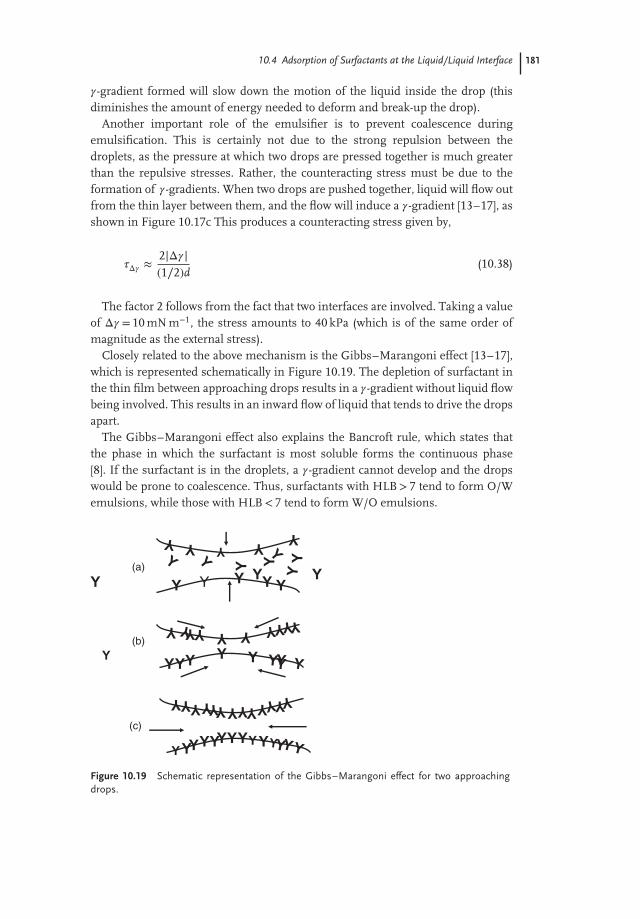
Closely related to the above mechanism is the Gibbs–Marangoni effect [13–17],which is represented schematically in Figure 10.19. The depletion of surfactant inthe thin film between approaching drops results in a 𝛾-gradient without liquid flowbeing involved. This results in an inward flow of liquid that tends to drive the dropsapart.

The Gibbs–Marangoni effect also explains the Bancroft rule, which states thatthe phase in which the surfactant is most soluble forms the continuous phase[8]. If the surfactant is in the droplets, a 𝛾-gradient cannot develop and the dropswould be prone to coalescence. Thus, surfactants with HLB> 7 tend to form O/Wemulsions, while those with HLB< 7 tend to form W/O emulsions.

(a)

(b)

(c)

Figure 10.19 Schematic representation of the Gibbs–Marangoni effect for two approachingdrops.


The Gibbs–Marangoni effect also explains the difference between surfactantsand polymers for emulsification. When compared to surfactants, polymers producelarger drops and also give a smaller value of 𝜀 at low concentrations (Figure 10.19).

Among various other factors that should be considered for emulsification mustbe included the disperse phase volume fraction 𝜙. An increase in 𝜙 leads to increasein droplet collision and hence coalescence during emulsification. Moreover, withan increase in 𝜙 the viscosity of the emulsion increases, and this may change theflow from being turbulent to being laminar (LV regime).

The presence of many particles results in a local increase in velocity gradients,which means that G is increased. In turbulent flow, an increase in 𝜙 will induceturbulence depression and this will result in larger droplets. Turbulence depressioncaused by added polymers tend to remove the small eddies and result in theformation of larger droplets.

If the mass ratio of the surfactant to the continuous phase is kept constant,an increase in 𝜙 will result in a decrease in surfactant concentration and hencean increase in 𝛾eq, resulting in larger droplets. However, if the mass ratio of thesurfactant to the disperse phase is kept constant, the above changes will be reversed.

At this point, general conclusions cannot be drawn since several of the above-mentioned mechanisms may come into play. Experiments using high-pressurehomogenisation at various 𝜑-values and constant initial mC (with TI regimechanging to TV at higher 𝜙) showed that, with increasing 𝜙 (>0.1), the resultingdroplet diameter was increased and the dependence on energy consumptionbecame weaker. Figure 10.20 shows a comparison of the average droplet diameterversus power consumption, using different emulsifying machines. The data show

1

0

−0.8

Colloid mill

log (d32

/μm)

1.5

0.025

30us

Ultra turrax

Homogeniser

4.5 5 6

p/Jm−3

7

Figure 10.20 Average droplet diametersobtained in various emulsifying machines asa function of energy consumption (p). Num-bers near the curves denote the viscosity

ratio (𝜆). Results for the homogeniser arefor 𝜙= 0.04 (solid line) and 𝜙= 0.3 (brokenline). us, ultrasonic generator.

10.5 Selection of Emulsifiers 183

that the smallest droplet diameters were obtained when using high-pressurehomogenisation.

10.5Selection of Emulsifiers

10.5.1The Hydrophilic–Lipophilic Balance (HLB) Concept

The selection of different surfactants in the preparation of either O/W or W/Oemulsions is often still made on an empirical basis. A semi-empirical scalefor selecting surfactants, the hydrophilic–lipophilic balance (HLB number) wasdeveloped by Griffin [18]. This scale is based on the relative percentage of hydrophilicto lipophilic (hydrophobic) groups in the surfactant molecule(s). For an O/Wemulsion droplet the hydrophobic chain resides in the oil phase, whereas thehydrophilic head group resides in the aqueous phase. In contrast, for a W/Oemulsion droplet the hydrophilic group(s) reside in the water droplet while thelipophilic groups reside in the hydrocarbon phase.

A guide to the selection of surfactants for particular applications is provided inTable 10.1. As the HLB number depends on the nature of the oil, the HLB numbersrequired to emulsify various oils are listed in Table 10.2, as an illustration.

The relative importance of the hydrophilic and lipophilic groups was firstrecognised when using mixtures of surfactants containing varying proportions of

Table 10.1 Summary of HLB ranges and their applications.

HLB range Application

3–6 W/O emulsifier7–9 Wetting agent8–18 O/W emulsifier13–15 Detergent15–18 Solubiliser

Table 10.2 Required HLB numbers to emulsify various oils.

Oil W/O emulsion O/W emulsion

Paraffin oil 4 10Beeswax 5 9Linolin, anhydrous 8 12Cyclohexane — 15Toluene — 15


Interfacial

Tension

1000

% Surfactant with high HLB

Emulsionstability

Dropletsize

Figure 10.21 Variation of emulsion stability, droplet size and interfacial tension with %surfactant with high HLB number.

low and high HLB numbers. The efficiency of any combination (as judged by phaseseparation) was found to pass a maximum when the blend contained a particularproportion of the surfactant with the higher HLB number. This is illustrated inFigure 10.21, which shows the variation of emulsion stability, droplet size andinterfacial tension with percentage surfactant with a high HLB number.

The average HLB number may be calculated from additivity,

HLB = x1HLB1 + x2HLB2 (10.39)

where x1 and x2 are the weight fractions of the two surfactants with HLB1 and HLB2.Griffin developed simple equations for calculating the HLB number of relatively

simple nonionic surfactants. For example, for a polyhydroxy fatty acid ester:

HLB = 20(

1 − SA

)(10.40)

where S is the saponification number of the ester and A is the acid number. Fora glyceryl monostearate, S= 161 and A= 198; the HLB is 3.8 (suitable for W/Oemulsion).

For a simple alcohol ethoxylate, the HLB number can be calculated from theweight percentage of EO (E) and polyhydric alcohol (P):

HLB = E + P5

(10.41)

If the surfactant contains PEO as the only hydrophilic group, the contributionfrom one OH group is neglected,

HLB = E5

(10.42)

For a nonionic surfactant C12H25–O–(CH2–CH2–O)6, the HLB is 12 (suitable forO/W emulsion).

The above simple equations cannot be used for surfactants containing propyleneoxide or butylene oxide; neither can they be applied for ionic surfactants. Davies[19, 20] devised a method for calculating the HLB number for surfactants fromtheir chemical formulae, using empirically determined group numbers that areassigned to various component groups. A summary of the group numbers for somesurfactants is provided in Table 10.3.

10.5 Selection of Emulsifiers 185

Table 10.3 HLB group numbers.

Group number

Hydrophilic–SO4Na+ 38.7–COO− 21.2–COONa 19.1N(tertiary amine) 9.4Ester (sorbitan ring) 6.8–O– 1.3CH–(sorbitan ring) 0.5

Lipophilic(–CH–), (–CH2–), CH3 0.475

Derived–CH2–CH2–O 0.33–CH2–CH2–CH2–O– −0.15

The HLB is given by the following empirical equation:

HLB = 7 +∑

(hydrophilic group Nos) −∑

(lipohilic group Nos) (10.43)

Davies has shown that the agreement between HLB numbers calculated fromthe above equation and those determined experimentally is quite satisfactory.

Various other procedures were developed to obtain a rough estimate of the HLBnumber. Griffin found good correlation between the cloud points of 5% solutionsof various ethoxylated surfactants and their HLB numbers. Davies [19, 20] alsoattempted to relate the HLB values to the selective coalescence rates of emulsions.Such correlations were not realised, however, as it was found that the emulsionstability – and even its type – depend to a large extent on the method of dispersingthe oil into the water, and vice versa. At best, the HLB number can only be used asa guide for selecting the optimum compositions of emulsifying agents.

Any pair of emulsifying agents that fall at opposite ends of the HLB scale – forexample, Tween 80 (sorbitan monooleate with 20 mol EO, HLB= 15) and Span80 (sorbitan monooleate, HLB= 5) – can be taken and used in various proportionsto cover a wide range of HLB numbers. The emulsions should be prepared inthe same fashion, with a few percent of the emulsifying blend. The stabilityof the emulsions can then be assessed at each HLB number, either from therate of coalescence or qualitatively by measuring the rate of oil separation. Inthis way it should be possible to determine the optimum HLB number for agiven oil. Subsequently, having found the most effective HLB value, various othersurfactant pairs can be compared at this HLB value to identify the most effectivepair.


10.5.2The Phase Inversion Temperature (PIT) Concept

Shinoda and coworkers [21, 22] found that many O/W emulsions stabilised withnonionic surfactants undergo a process of inversion at a critical temperature,termed the phase inversion temperature (PIT). The PIT can be determined byfollowing the emulsion conductivity (a small amount of electrolyte is added toincrease the sensitivity) as a function of temperature. The conductivity of the O/Wemulsion increases with an increase of temperature until the PIT is reached, abovewhich there will be a rapid reduction in conductivity (a W/O emulsion is formed).Shinoda and coworkers found that the PIT is influenced by the HLB number ofthe surfactant. In addition, the size of the emulsion droplets was found to dependon the temperature and the HLB number of the emulsifiers, with the dropletsbeing less stable towards coalescence when close to the PIT. However, a rapidcooling of the emulsion allows the production of a stable system. Relatively stableO/W emulsions were obtained when the PIT of the system was 20–65 ◦C higherthan the storage temperature. Emulsions prepared at a temperature just below thePIT, followed by rapid cooling, generally have smaller droplet sizes. This effect canbe understood by considering the change in interfacial tension with temperature,as illustrated in Figure 10.22. The interfacial tension decreases with an increaseof temperature to reach a minimum when close to the PIT, after which thetension increases.

Thus, droplets prepared close to the PIT will be smaller than those preparedat lower temperatures. These droplets are relatively unstable towards coalescencenear the PIT, although by rapid cooling of the emulsion the smaller size can beretained. This procedure may be applied to prepare mini (nano) emulsions.

PIT

Temperature Increase

0.01

0.1

1

10

20

𝛾/mNm−1

Figure 10.22 Variation of interfacial tension with temperature increase for an O/Wemulsion.

10.6 Creaming or Sedimentation of Emulsions 187

Whilst the optimum stability of the emulsion was found to be relatively insensitiveto changes in the HLB value or the PIT of the emulsifier, its instability was verysensitive to the PIT of the system.

It is essential, therefore to measure the PIT of the emulsion as a whole (with allother ingredients).

At a given HLB value, the stability of emulsions against coalescence is increasedmarkedly as the molar mass of both the hydrophilic and lipophilic components isincreased. An enhanced stability using high-molecular-weight (polymeric) surfac-tants can be understood by considering the steric repulsion, which produces morestable films. Films produced using macromolecular surfactants resist thinning anddisruption, thus reducing the possibility of coalescence. The emulsions showedmaximum stability when the distribution of the PEO chains was broad. The cloudpoint was lower but the PIT was higher than in the corresponding case for narrowsize distributions. Hence, the PIT and HLB number are directly related parameters.

As the addition of electrolytes reduces the PIT, an emulsifier with a higher PITvalue will be required when preparing emulsions in the presence of electrolytes.Electrolytes cause dehydration of the PEO chains which, in effect, reduces thecloud point of the nonionic surfactant; this must be compensated for by using asurfactant with a higher HLB. The optimum PIT of the emulsifier is fixed if thestorage temperature is fixed.

Measurement of the PIT can at best be used as a guide for the preparation ofstable emulsions. Any assessments of stability should be evaluated by followingthe droplet size distribution as a function of time, using a Coulter counter orlight-diffraction techniques. Following the rheology of the emulsion as a functionof time and temperature may also be used to assess the stability against coalescence.Care should be taken when analysing the rheological results as coalescence leads toan increase in droplet size that is usually followed by a reduction in the viscosity ofthe emulsion. This trend is only observed if the coalescence is not accompanied byflocculation of the emulsion droplets (which results in an increase in the viscosity).Ostwald ripening can also complicate the analysis of rheological data.

10.6Creaming or Sedimentation of Emulsions

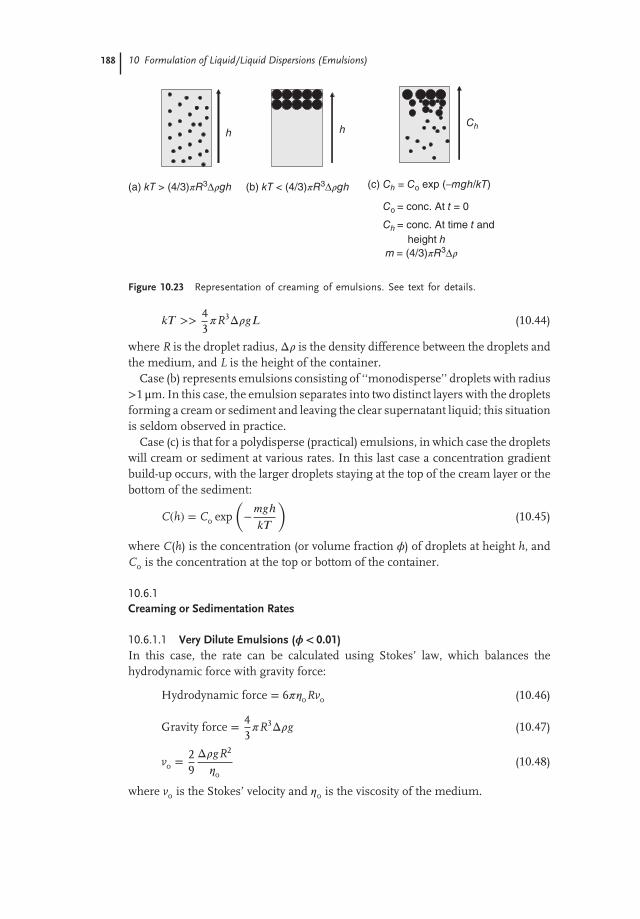
This is the result of gravity, when the density of the droplets and the medium arenot equal. When the density of the disperse phase is lower than that of the medium,creaming occurs, whereas if the density of the disperse phase is higher than that ofthe medium, sedimentation occurs. A schematic representation for the creamingof emulsions in three cases is shown in Figure 10.23 [1–3].

Case (a) represents the situation for small droplets (<0.1 μm, i.e., nanoemul-sions), whereby the Brownian diffusion kT (where k is the Boltzmann constant andT is the absolute temperature) exceeds the force of gravity (mass× acceleration dueto gravity, g):


h hCh

(a) kT > (4/3)𝜋R3Δ𝜌gh (b) kT < (4/3)𝜋R3Δ𝜌gh (c) Ch = Co exp (−mgh/kT)

Co = conc. At t = 0

m = (4/3)𝜋R3Δ𝜌

Ch = conc. At time t and

height h

Figure 10.23 Representation of creaming of emulsions. See text for details.

𝑘𝑇 >>43𝜋R3Δ𝜌𝑔𝐿 (10.44)

where R is the droplet radius, Δ𝜌 is the density difference between the droplets andthe medium, and L is the height of the container.

Case (b) represents emulsions consisting of ‘‘monodisperse’’ droplets with radius>1 μm. In this case, the emulsion separates into two distinct layers with the dropletsforming a cream or sediment and leaving the clear supernatant liquid; this situationis seldom observed in practice.

Case (c) is that for a polydisperse (practical) emulsions, in which case the dropletswill cream or sediment at various rates. In this last case a concentration gradientbuild-up occurs, with the larger droplets staying at the top of the cream layer or thebottom of the sediment:

C(h) = Co exp

(−𝑚𝑔ℎ

𝑘𝑇

)(10.45)

where C(h) is the concentration (or volume fraction 𝜙) of droplets at height h, andCo is the concentration at the top or bottom of the container.

10.6.1Creaming or Sedimentation Rates

10.6.1.1 Very Dilute Emulsions (𝝓< 0.01)In this case, the rate can be calculated using Stokes’ law, which balances thehydrodynamic force with gravity force:

Hydrodynamic force = 6𝜋𝜂oRvo (10.46)

Gravity force = 43𝜋R3Δ𝜌𝑔 (10.47)

vo = 29Δ𝜌𝑔R2

𝜂o(10.48)

where vo is the Stokes’ velocity and 𝜂o is the viscosity of the medium.


For an O/W emulsion withΔρ= 0.2 in water (ηo ∼ 10−3 Pa⋅s), the rate of creamingor sedimentation is ∼4.4× 10−5 m s−1 for 10 μm droplets, and ∼4.4× 0−7 m s−1 for1 μm droplets. This means that in a 0.1 m container, creaming or sedimentation ofthe 10 μm droplets will be complete in ∼0.6 h, whereas for the 1 μm droplets thiswill take ∼60 h.

10.6.1.2 Moderately Concentrated Emulsions (0.2<𝝋< 0.1)In this case, account must be taken of the hydrodynamic interaction between thedroplets, which reduces the Stokes velocity to a value v given, by the followingexpression [23]:

v = vo(1 − 𝑘𝜑) (10.49)

where k is a constant that accounts for hydrodynamic interaction. k is on the orderof 6.5, which means that the rate of creaming or sedimentation is reduced by about65%.

10.6.1.3 Concentrated Emulsions (𝝋> 0.2)The rate of creaming or sedimentation becomes a complex function of 𝜙, asillustrated in Figure 10.24, which also shows the change of relative viscosity 𝜂r

with 𝜙.As can be seen from Figure 10.24, v decreases with the increase in 𝜙 and

ultimately approaches zero when 𝜙 exceeds a critical value, 𝜑p, which is theso-called ‘‘maximum packing fraction.’’ The value of 𝜙p for monodisperse ‘‘hard-spheres’’ ranges from 0.64 (for random packing) to 0.74 for hexagonal packing, butexceeds 0.74 for polydisperse systems. For emulsions which are deformable, 𝜙p

can be much larger than 0.74.The data in Figure 10.24 also show that when 𝜙 approaches 𝜙p, 𝜂r approaches

∞. In practice, most emulsions are prepared at 𝜙-values well below 𝜙p (usually inthe range of 0.2–0.5), and under these conditions creaming or sedimentation isthe rule rather than the exception. Several procedures may be applied to reduce oreliminate creaming or sedimentation, and these are discussed below.

v𝜂r

[𝜂]

1

𝜙 𝜙

𝜙p 𝜙p

Figure 10.24 Variation of v and 𝜂r with 𝜑.


10.6.2Prevention of Creaming or Sedimentation

10.6.2.1 Matching the Density of Oil and Aqueous PhasesClearly, ifΔ𝜌= 0, v= 0; however, this method is seldom practical. Density matching,if possible, only occurs at one temperature.

10.6.2.2 Reduction of Droplet SizeSince the gravity force is proportional to R3, then if R is reduced by a factor of 10, thegravity force is reduced by 1000. Below a certain droplet size (which also dependson the density difference between oil and water), the Brownian diffusion mayexceed gravity and creaming or sedimentation is prevented. This is the principleof formulation of nanoemulsions (with size range 20–200 nm) that may show verylittle or no creaming or sedimentation. The same applies for microemulsions (sizerange 5–50 nm).

10.6.2.3 Use of ‘Thickeners’These are high-molecular-weight polymers, either natural or synthetic, such asxanthan gum, hydroxyethyl cellulose, alginates, and carrageenans. In order tounderstand the role of these ‘‘thickeners,’’ the gravitational stresses exerted duringcreaming or sedimentation should be considered:

stress = massof drop × accelerationdue togravity = 43𝜋R3Δ𝜌𝑔 (10.50)

To overcome such stress, needs a restoring force is needed:

Restoringforce = areaof drop × stressof drop = 4𝜋R2𝜎p (10.51)

Thus, the stress exerted by the droplet 𝜎p is given by,

𝜎p = Δ𝜌𝑅𝑔3

(10.52)

Simple calculation shows that 𝜎p is in the range 10−3 to 10−1 Pa, which impliesthat for prediction of creaming or sedimentation it is necessary to measure theviscosity at such low stresses. This can be achieved by using constant stress orcreep measurements.

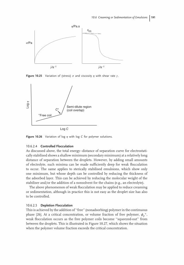
The above-described ‘‘thickeners’’ satisfy the criteria for obtaining very highviscosities at low stresses or shear rates. This can be illustrated from plots ofshear stress 𝜎 and viscosity 𝜂 versus shear rate 𝛾 (or shear stress), as shown inFigure 10.25. These systems are described as ‘‘pseudoplastic’’ or shear thinning.The low shear (residual or zero shear rate) viscosity 𝜂(0) can reach several thousandPa⋅s, and such high values prevent creaming or sedimentation [24, 25].

The above-described behaviour is obtained above a critical polymer concentration(C*), which can be located from plots of log 𝜂 versus log C, as is illustrated inFigure 10.26. Below C*, the log 𝜂–log C curve has a slope in the region of 1,whereas above C* the slope of the line exceeds 3. In most cases a good correlationbetween the rate of creaming or sedimentation and 𝜂(0) is obtained.


𝛾/s−1 𝛾/s−1

𝜎/Pa

𝜂/Pa.s𝜂

(0)

Figure 10.25 Variation of (stress) 𝜎 and viscosity 𝜂 with shear rate 𝛾 .

Log 𝜂

Log C

C*

‘’Free coil

Semi-dilute region(coil overlap)

Figure 10.26 Variation of log 𝜂 with log C for polymer solutions.

10.6.2.4 Controlled FlocculationAs discussed above, the total energy–distance of separation curve for electrostati-cally stabilised shows a shallow minimum (secondary minimum) at a relatively longdistance of separation between the droplets. However, by adding small amountsof electrolyte, such minima can be made sufficiently deep for weak flocculationto occur. The same applies to sterically stabilised emulsions, which show onlyone minimum, but whose depth can be controlled by reducing the thickness ofthe adsorbed layer. This can be achieved by reducing the molecular weight of thestabiliser and/or the addition of a nonsolvent for the chains (e.g., an electrolyte).

The above phenomenon of weak flocculation may be applied to reduce creamingor sedimentation, although in practice this is not easy as the droplet size has alsoto be controlled.

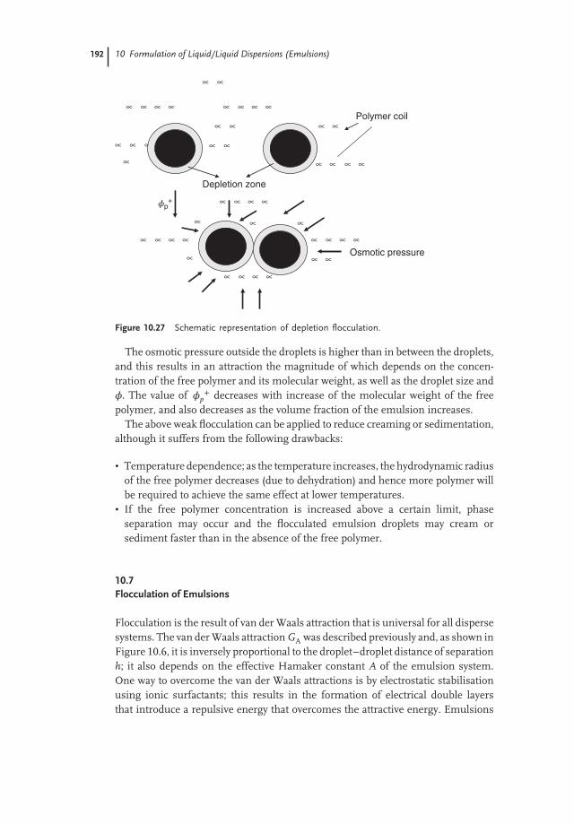
10.6.2.5 Depletion FlocculationThis is achieved by the addition of ‘‘free’’ (nonadsorbing) polymer in the continuousphase [26]. At a critical concentration, or volume fraction of free polymer, 𝜙p

+,weak flocculation occurs as the free polymer coils become ‘‘squeezed-out’’ frombetween the droplets. This is illustrated in Figure 10.27, which shows the situationwhen the polymer volume fraction exceeds the critical concentration.


∝

Depletion zone

Osmotic pressure

Polymer coil∝ ∝ ∝

∝ ∝

∝

∝ ∝ ∝

∝ ∝

∝ ∝

∝ ∝

∝ ∝

∝ ∝ ∝

∝ ∝

∝

∝ ∝ ∝ ∝

𝜙p+

∝ ∝ ∝ ∝

∝ ∝ ∝ ∝

∝ ∝∝

∝

∝ ∝

∝ ∝ ∝ ∝

Figure 10.27 Schematic representation of depletion flocculation.

The osmotic pressure outside the droplets is higher than in between the droplets,and this results in an attraction the magnitude of which depends on the concen-tration of the free polymer and its molecular weight, as well as the droplet size and𝜙. The value of 𝜙p

+ decreases with increase of the molecular weight of the freepolymer, and also decreases as the volume fraction of the emulsion increases.

The above weak flocculation can be applied to reduce creaming or sedimentation,although it suffers from the following drawbacks:

• Temperature dependence; as the temperature increases, the hydrodynamic radiusof the free polymer decreases (due to dehydration) and hence more polymer willbe required to achieve the same effect at lower temperatures.

• If the free polymer concentration is increased above a certain limit, phaseseparation may occur and the flocculated emulsion droplets may cream orsediment faster than in the absence of the free polymer.

10.7Flocculation of Emulsions

Flocculation is the result of van der Waals attraction that is universal for all dispersesystems. The van der Waals attraction GA was described previously and, as shown inFigure 10.6, it is inversely proportional to the droplet–droplet distance of separationh; it also depends on the effective Hamaker constant A of the emulsion system.One way to overcome the van der Waals attractions is by electrostatic stabilisationusing ionic surfactants; this results in the formation of electrical double layersthat introduce a repulsive energy that overcomes the attractive energy. Emulsions

10.7 Flocculation of Emulsions 193

stabilised by electrostatic repulsion become flocculated at intermediate electrolyteconcentrations (see below). The second and most effective method of overcomingflocculation is by ‘‘steric stabilisation’’ using nonionic surfactants or polymers.Stability may be maintained in electrolyte solutions (as high as 1 mol dm−3,depending on the nature of the electrolyte) and up to high temperatures (in excessof 50 ◦C), provided that the stabilising chains (e.g., PEO) are still in better than𝜃-conditions (𝜒 < 0.5).

10.7.1Mechanism of Emulsion Flocculation

This can occur if the energy barrier is small or absent (for electrostatically stabilisedemulsions) or when the stabilising chains reach poor solvency (for stericallystabilised emulsions, that is if 𝜒 > 0.5). For convenience, the flocculation ofelectrostatically and sterically stabilised emulsions will be discussed separately.

10.7.1.1 Flocculation of Electrostatically Stabilised EmulsionsAs discussed above, the condition for kinetic stability is Gmax > 25 kT since, whenGmax < 5 kT flocculation will occur. Two types of flocculation kinetics may bedistinguished: fast flocculation with no energy barrier; and slow flocculation whenan energy barrier exists.

The fast flocculation kinetics was treated by Smoluchowski [27], who consideredthe process to be represented by second-order kinetics and to be simply diffusion-controlled. The number of particles n at any time t may be related to the finalnumber no (at t= 0) by the following expression:

n =no

1 + knot(10.53)

where k is the rate constant for fast flocculation that is related to the diffusioncoefficient of the particles D, that is,

k = 8𝜋𝐷𝑅 (10.54)

where D is given by the Stokes–Einstein equation,

D = 𝑘𝑇

6𝜋𝜂𝑅(10.55)

Combining Equations (10.54) and (10.55),

k = 43𝑘𝑇

𝜂= 5.5 × 10−18m3s−1forwaterat25oC (10.56)

The half-life t1/2 (n= (1/2) no) can be calculated at various no or volume fraction𝜙, as given in Table 10.4.

The slow flocculation kinetics was treated by Fuchs [28] who related the rateconstant k to the Smoluchowski rate by the stability constant W:

W =ko

k(10.57)


Table 10.4 Half-life of emulsion flocculation.

R (𝛍m) 𝝓

10−5 10−2 10−1 5× 10−1

0.1 765 s 76 ms 7.6 ms 1.5 ms1.0 21 h 76 s 7.6 s 1.5 s10.0 4 mo 21 h 2 h 25 m

where W is related to Gmax by the following expression [29],

W = 12

exp

(Gmax

𝑘𝑇

)(10.58)

Since Gmax is determined by the salt concentration C and valency, it is possibleto derive an expression relating W to C and Z,

log W = −2.06 × 109

(R𝛾2

Z2

)log C (10.59)

where 𝛾 is a function that is determined by the surface potential 𝜓o,

𝛾 =

[exp

(𝑍𝑒𝜓o∕𝑘𝑇

)− 1

exp(𝑍𝐸𝜓o∕𝑘𝑇 ) + 1

](10.60)

Plots of log W versus log C are shown in Figure 10.28. The condition log W = 0(W = 1) is the onset of fast flocculation. The electrolyte concentration at this pointdefines the critical flocculation concentration (CFC). Above the CFC, W < 1 (dueto the contribution of van der Waals attractions which accelerate the rate abovethe Smoluchowski value). Below the CFC, W > 1 and it increases with a decrease

Log W

W = 1 0

2:2 Electrolyte 1:1 Electrolyte

10−3 10−2

Log C

10−1

Figure 10.28 Log W –log C curves for electrostatically stabilised emulsions.

10.7 Flocculation of Emulsions 195

of electrolyte concentration. The data in Figure 10.28 also show that the CFCdecreases with increase of valency, in accordance to the Schultze–Hardy rule.

Another mechanism of flocculation is that involving the secondary minimum(Gmin), which typically is a few kT units. In this case the flocculation is weakand reversible, and hence both the rate of flocculation (forward rate kf) anddeflocculation (backward rate kb) must be considered. The rate of decrease ofparticle number with time is given by the expression,

−dndt

= −kf n2 + kbn (10.61)

The backward reaction (break-up of weak flocs) reduces the overall rate offlocculation.

10.7.1.2 Flocculation of Sterically Stabilised EmulsionsThis occurs when the solvency of the medium for the chain becomes worse than a𝜃-solvent (𝜒 > 0.5). Under these conditions, Gmix becomes negative (i.e., attractive)and a deep minimum is produced that results in catastrophic flocculation (this isreferred to as incipient flocculation). This is shown schematically in Figure 10.29.With many systems a good correlation between the flocculation point and the𝜃-point is obtained.

For example, the emulsion will flocculate at a temperature (referred to as thecritical flocculation temperature; CFT) that is equal to the 𝜃-temperature of thestabilising chain. The emulsion may flocculate at a critical volume fraction (CFV)of a nonsolvent, which is equal to the volume of nonsolvent that brings it to a𝜃-solvent.

G

h 2𝛿 2𝛿 h

GelGel

Gmix

GT

GT

GA

Gmix

Gmin𝜒 < 0.5 𝜒 > 0.5

Reducesolvency

𝛿𝛿

Figure 10.29 Schematic representation of flocculation of sterically stabilised emulsions.


10.8General Rules for Reducing (Eliminating) Flocculation

10.8.1Charge-Stabilised Emulsions (e.g., Using Ionic Surfactants)

The most important criterion is to make Gmax as high as possible; this is achievedby three main conditions: (i) high surface or zeta-potential; (ii) low electrolyteconcentration; and (iii) low valency of ions.

10.8.2Sterically Stabilised Emulsions

Four main criteria are necessary:

• Complete coverage of the droplets by the stabilising chains.• A firm attachment (strong anchoring) of the chains to the droplets. This requires

the chains to be insoluble in the medium and soluble in the oil. However, thisis incompatible with stabilisation which requires a chain that is soluble in themedium and strongly solvated by its molecules. These conflicting requirementsare solved by the use of A-B, A-B-A block or BAn graft copolymers (B is the‘‘anchor’’ chain and A is the stabilising chain(s)). Examples of the B chains forO/W emulsions are polystyrene, PMMA, PPO and alkyl PPO. For the A chain(s),PEO or polyvinyl alcohol are good examples. For W/O emulsions, PEO can formthe B chain, whereas the A chain(s) could be polyhydroxy stearic acid (PHS)which is strongly solvated by most oils.

• Thick adsorbed layers; the adsorbed layer thickness should be in the region of5–10 nm. This means that the molecular weight of the stabilising chains couldbe in the region of 1000–5000 Da.

• The stabilising chain should be maintained in good solvent conditions (𝜒 < 0.5)under all conditions of temperature changes on storage.

10.9Ostwald Ripening

The driving force for Ostwald ripening is the difference in solubility between thesmall and large droplets (the smaller droplets have a higher Laplace pressure and ahigher solubility than the larger droplets). This is illustrated in Figure 10.30, whereR1 decreases and R2 increases as a result of diffusion of molecules from the smallerto the larger droplets.

The difference in chemical potential between different sized droplets was givenby Lord Kelvin [30],

S(r) = S(∞) exp

(2𝛾Vm

𝑟𝑅𝑇

)(10.62)

10.9 Ostwald Ripening 197

r1r2

Molecular

Diffusion of oil

S1 = 2𝛾/r1S2 = 2𝛾/r2

Figure 10.30 Schematic representation of Ostwald ripening.

where S(r) is the solubility surrounding a particle of radius r, S(∞) is the bulksolubility, Vm is the molar volume of the dispersed phase, R is the gas constant,and T is the absolute temperature.

The quantity (2 𝛾 Vm/ RT) is termed the characteristic length, and has an order of∼1 nm or less, indicating that the difference in solubility of a 1 μm droplet is of theorder of 0.1%, or less. In theory, Ostwald ripening should lead to the condensationof all droplets into a single drop; however, this does not occur in practice as the rateof growth decreases with increases in droplet size.

For two droplets with radii r1 and r2 (r1 < r2),

𝑅𝑇

Vm

ln

[S(r1

)S(r2)

]= 2𝛾

[1r1

− 1r2

](10.63)

Equation (10.63) shows that the larger the difference between r1 and r2, thehigher the rate of Ostwald ripening.

Ostwald ripening can be quantitatively assessed from plots of the cube of theradius versus time t [31, 32],

r3 = 89

[S (∞) 𝛾VmD

𝜌𝑅𝑇

]t (10.64)

where D is the diffusion coefficient of the disperse phase in the continuous phaseand 𝜌 is the density of the disperse phase.

Several methods may be applied to reduce Ostwald ripening [33–35]:

(i) The addition of a second disperse phase component which is insoluble inthe continuous medium (e.g., squalane). In this case, partitioning betweendifferent droplet sizes occurs, with the component having a low solubilityexpected to be concentrated in the smaller droplets. During Ostwald ripeningin a two-component system, equilibrium is established when the differencein chemical potential between different size droplets (which results fromcurvature effects) is balanced by the difference in chemical potential resultingfrom partitioning of the two components. This effect reduces further growthof droplets.

(ii) Modification of the interfacial film at the O/W interface. According to Equation(10.64), a reduction in 𝛾 will result in a reduction of the Ostwald ripeningrate. By using surfactants that are strongly adsorbed at the O/W interface(i.e., polymeric surfactants), and which do not desorb during ripening (by


choosing a molecule that is insoluble in the continuous phase), the rate couldbe significantly reduced. An increase in the surface dilational modulus 𝜀 (=d𝛾/dln A) and a decrease in 𝛾 would be observed for the shrinking drop, andthis would tend to reduce further growth.

A-B-A block copolymers such as PHS-PEO-PHS (which is soluble in the oildroplets, but insoluble in water) can be used to achieve the above effect. Similareffects can also be obtained using a graft copolymer of hydrophobically modified

inulin, namely INUTEC®

SP1 (ORAFTI, Belgium). This polymeric surfactantadsorbs with several alkyl chains (which may dissolve in the oil phase), leavingloops and tails of strongly hydrated inulin (polyfructose) chains. The moleculehas a limited solubility in water and hence it resides at the O/W interface. Thesepolymeric emulsifiers enhance the Gibbs elasticity, thus significantly reducing theOstwald ripening rate.

10.10Emulsion Coalescence

When two emulsion droplets come into close contact in a floc or creamed layer,or during Brownian diffusion, thinning and disruption of the liquid film mayoccur that results in eventual rupture. On close approach of the droplets, filmthickness fluctuations may occur; alternatively, the liquid surfaces may undergosome fluctuations to form surface waves, as illustrated in Figure 10.31. Thesesurface waves may grow in amplitude and the apices may join as a result of thestrong van der Waals attractions (at the apex, the film thickness is the smallest). Thesame applies if the film thins to a small value (critical thickness for coalescence)

A very useful concept was introduced by Deryaguin [36], who suggested thata ‘‘Disjoining Pressure’’ 𝜋(h) is produced in the film which balances the excessnormal pressure,

𝜋(h) = P(h) − Po (10.65)

where P(h) is the pressure of a film with thickness h, and Po is the pressure of asufficiently thick film such that the net interaction free energy is zero.𝜋(h) may be equated to the net force (or energy) per unit area acting across the

film,

𝜋(h) = −dGT

dh(10.66)

where GT is the total interaction energy in the film.

Figure 10.31 Schematic representation of surface fluctuations.

10.10 Emulsion Coalescence 199

𝜋(h) is composed of three contributions due to electrostatic repulsion (𝜋E), stericrepulsion (𝜋s) and van der Waals attractions (𝜋A),

𝜋(h) = 𝜋E + 𝜋s + 𝜋A (10.67)

In order to produce a stable film 𝜋E +𝜋s >𝜋A, and this is the driving forcefor the prevention of coalescence, which can be achieved by two mechanismsand their combination: (i) increased repulsion, both electrostatic and steric; and(ii) dampening of the fluctuation by enhancing the Gibbs elasticity. In general,smaller droplets are less susceptible to surface fluctuations and hence coalescenceis reduced; this explains the high stability of nanoemulsions.

Several methods may be applied to achieve the above effects:

• Use of mixed surfactant films: In many cases the used of mixed surfactants (e.g.,anionic and nonionic or long chain alcohols) can reduce coalescence as a resultof several effects: a high Gibbs elasticity; high surface viscosity; and hindereddiffusion of surfactant molecules from the film.

• Formation of lamellar liquid crystalline phases at the O/W interface: Thismechanism, as suggested by Friberg and coworkers [37], proposed that surfactantor mixed surfactant film can produce several bilayers that ‘‘wrap’’ the droplets.As a result of these multilayer structures, the potential drop is shifted tolonger distances, thus reducing the van der Waals attractions. A schematicrepresentation of the role of liquid crystals is shown in Figure 10.32, whichillustrates the difference between having a monomolecular layer and a multilayer,as is the case with liquid crystals.

For coalescence to occur, these multilayers have to be removed ‘two-by-two’ andthis forms an energy barrier preventing coalescence.

oilWater Water

Water WaterMO

Water Water

oil

Om

Om

O

mw w wO

mw O

mw

wO

mw O

m

w o w o ww o w oooo

w

Upper part monomolecular layer

Lower part presence of liquid crystalline phases

Figure 10.32 Schematic representation of the role of liquid crystalline phases.


10.10.1Rate of Coalescence

Since film drainage and rupture is a kinetic process, coalescence is also a kineticprocess. If the number of particles n (flocculated or not) is measured at time t,

n = nt + nvm (10.68)

where nt is the number of primary particles remaining, and n is the number ofaggregates consisting of m separate particles.

For studying emulsion coalescence, it is important to consider the rate constantof flocculation and coalescence. If coalescence is the dominant factor, then the rateK follows a first-order kinetics,

n =no

𝐾𝑡[1 + exp(−𝐾𝑡)] (10.69)

which shows that a plot of log n versus t should give a straight line from which Kcan be calculated.

10.11Phase Inversion

The phase inversion of emulsions can be one of two types: (i) transitional inversion,which is induced by changing facers which affect the HLB of the system (e.g.,temperature and/or electrolyte concentration); and (ii) catastrophic inversion, whichis induced by increasing the volume fraction of the disperse phase.

Catastrophic inversion is illustrated in Figure 10.33, which shows the variation ofviscosity and conductivity with the oil volume fraction 𝜙. As can be seen, inversionoccurs at a critical 𝜙, which may be identified with the maximum packing fraction.

O/W

W/O

𝜑cr

𝜑

𝜅

𝜂

𝜂

𝜂

𝜅

𝜅

Figure 10.33 Variation of conductivity and viscosity with volume fraction of oil.

References 201

At 𝜙cr, 𝜂 suddenly decreases as the inverted W/O emulsion has a much lowervolume fraction. 𝜅 also decreases sharply at the inversion point as the continuousphase is now oil.

Earlier theories of phase inversion were based on packing parameters. When 𝜑

exceeds the maximum packing (∼0.64 for random packing and ∼0.74 for hexagonalpacking of monodisperse spheres; for polydisperse systems, the maximum packingexceeds 0.74), inversion occurs. However, these theories are inadequate as manyemulsions invert at φ values well below the maximum packing as a result of thechange in surfactant characteristics with variation of conditions. For example, whenusing a nonionic surfactant based on PEO the latter chain changes its solvation byincrease of temperature and/or the addition of electrolyte. Many emulsions showphase inversion at a critical temperature (the PIT) that depends on the HLB numberof the surfactant as well as the presence of electrolytes. By increasing temperatureand/or addition of electrolyte, the PEO chains become dehydrated and finally moresoluble in the oil phase. Under these conditions, the O/W emulsion will invertto a W/O emulsion. The above dehydration effect amounts to a decrease in theHLB number, and when the latter reaches a value that is more suitable for a W/Oemulsion then inversion will occur. At present, however, there is no quantitativetheory that accounts for phase inversion of emulsions.

References

1. Tadros, T.F. and Vincent, B. (1983) inEncyclopedia of Emulsion Technology (ed.P. Becher), Marcel Dekker, New York.

2. Tadros, T. (ed.) (2013) Emulsion Forma-tion and Stability, Wiley-VCH VerlagGmbH, Weinheim.

3. Tadros, T. (2005) Applied Surfactants,Wiley-VCH Verlag GmbH, Weinheim.

4. Hamaker, H.C. (1937) Physica (Utrecht),4, 1058.

5. Deryaguin, B.V. and Landau, L. (1941)Acta Physicochem. USSR, 14, 633.

6. Verwey, E.J.W. and Overbeek, J.T.G.(1948) Theory of Stability of LyophobicColloids, Elsevier, Amsterdam.

7. Napper, D.H. (1983) Polymeric Stabil-isation of Dispersions, Academic Press,London.

8. Walstra, P. and Smolders, P.E.A. (1998)in Modern Aspects of Emulsions (ed. B.P.Binks), The Royal Society of Chemistry,Cambridge.

9. Stone, H.A. (1994) Annu. Rev. FluidMech., 226, 95.

10. Wierenga, J.A., ven Dieren, F., Janssen,J.J.M., and Agterof, W.G.M. (1996)Trans. Inst. Chem. Eng., 74-A, 554.

11. Levich, V.G. (1962) PhysicochemicalHydrodynamics, Prentice-Hall, Engle-wood Cliffs, NJ.

12. Davis, J.T. (1972) Turbulent Phenomena,Academic Press, London.

13. Lucasses-Reynders, E.H. (1996) in Ency-clopedia of Emulsion Technology (ed. P.Becher), Marcel Dekker, New York.

14. Graham, D.E. and Phillips, M.C. (1979)J. Colloid Interface Sci., 70, 415.

15. Lucassen-Reynders, E.H. (1994) ColloidsSurf., A91, 79.

16. Lucassen, J. (1981) in Anionic Surfactants(ed. E.H. Lucassen-Reynders), MarcelDekker, New York.

17. van den Tempel, M. (1960) Proc. Int.Congr. Surf. Activity, 2, 573.

18. Griffin, W.C. J. Cosmet. Chemists, 1,311(1949); 5, 249 (1954).

19. Davies, J.T. (1959) Proc. Int. Congr. Surf.Activity, 1, 426.

20. Davies, J.T. and Rideal, E.K. (1961) Inter-facial Phenomena, Academic Press, NewYork.

21. Shinoda, K. (1967) J. Colloid InterfaceSci., 25, 396.


22. Shinoda, K. and Saito, H. (1969) J.Colloid Interface Sci., 30, 258.

23. Batchelor, G.K. (1972) J. Fluid. Mech.,52, 245.

24. Buscall, R., Goodwin, J.W., Ottewill,R.H., and Tadros, T.F. (1982) J. ColloidInterface Sci., 85, 78.

25. Tadros, T. (2010) Rheology of Dispersions,Wiley-VCH Verlag GmbH, Weinheim.

26. Asakura, S. and Osawa, F. (1954) J.Phys. Chem., 22, 1255; J. Polym. Sci.,1958, 33, 183.

27. Smoluchowski, M.V. (1927) Z. Phys.Chem., 92, 129.

28. Fuchs, N. (1936) Z. Phys., 89, 736.29. Reerink, H. and Overbeek, J.T.G. (1954)

Disc. Faraday Soc., 18, 74.30. Thompson, W. (Lord Kelvin) (1871) Phi-

los. Mag., 42, 448.

31. Lifshitz, I.M. and Slesov, V.V. (1959)Sov. Phys. JETP, 35, 331.

32. Wagner, C. (1961) Z. Electrochem., 35,581.

33. Kabalanov, A.S. and Shchukin, E.D.(1992) Adv. Colloid Interface Sci., 38, 69.

34. Kabalanov, A.S. (1994) Langmuir, 10,680.

35. Weers, J.G. (1998) in Modern Aspectsof Emulsion Science (ed. B.P. Binks),Royal Society of Chemistry Publication,Cambridge.

36. Deryaguin, B.V. and Scherbaker, R.L.(1961) Kolloid Zh., 23, 33.

37. Friberg, S., Jansson, P.O., andCederberg, E. (1976) J. Colloid InterfaceSci., 55, 614.

formulation of disperse systems (science and technology) || formulation of liquid/liquid dispersions...

Documents