formulary electric power engineering
TRANSCRIPT

Institute of Electric Power Systems
Electric Power Engineering Section
Prof. Dr.-Ing. habil. L. Hofmann
Leibniz University Hanover
Institute of Electric Power Systems
Electric Power Engineering Section
Formulary
Electric Power Engineering
Lutz Hofmann
6th Edition, September 2020

© Institute of Electric Power Systems
Power Engineering Section
Leibniz University Hannover
Prof. Dr.-Ing. habil. L. Hofmann
www.ifes.uni-hannover.de

Institute of Electric Power Systems
Electric Power Engineering Section
Prof. Dr.-Ing. habil. L. Hofmann
Preface
This formulary includes definitions and formulas from lectures of the Electric Power Engi-
neering Section of the Institute of Electric Power Systems (IfES) at Leibniz University Han-
over, Germany.
The formulary introduces basic mathematical knowledge and definitions as well as elemen-
tary definitions of electric power engineering using typical German symbols, e.g. for com-
plex rotating and stationary phasors, the passive sign convention or multi-port representation
of electrical devices. From the voltage equations of the symmetrical three-phase power sys-
tem, the single-phase equivalent circuit diagram is derived using the symmetry conditions.
The presentation of the methodology with the symmetrical components enables the reader
to easily calculate unbalanced operating states as a result of, e.g., unbalanced short circuits
or interruptions by a fault-specific interconnection of the positive-, negative- and zero-se-
quence systems.
For the system-defining equipment of electrical power systems, such as synchronous ma-
chines, induction machines, equivalent networks, transformers and lines, the respective pos-
itive-, negative- and zero-sequence equivalent circuits for the calculation of the steady-state
operating behavior are presented and, if necessary, supplemented by equivalent circuits for
the transient and subtransient operating behavior.
Finally, basic methods for network calculation, equipment design and network control are
presented, such as a method for the calculation of current distributions in medium- and low-
voltage networks, stability analysis of the single machine problem, frequency control based
on the dynamic balance model as well as short-circuit current calculation, especially accord-
ing to IEC EN 60909. Furthermore, the calculation of line-to-ground faults in networks with
different types of star point grounding is presented.
The authors hope that this collection of formulae will not only serve students as an assistance
in their exams and lecture-accompanying exercises but will also be of use in their future
professional life.
This is the sixth edition of the formulary provided by the Electric Power Engineering Section
in English language. Suggestions for this edition are welcome and can be submitted to
Hannover, September 2020 Lutz Hofmann and the research assistants of the
Electric Power Engineering Section of IfES

Institut für Elektrische Energiesysteme
Fachgebiet Elektrische Energieversorgung
Prof. Dr.-Ing. habil. L. Hofmann
Table of contents
1 Symbols and Abbreviations ....................................................................................... IV
2 Fundamentals ................................................................................................................ 1
2.1 Instantaneous Values and Phasor Representation ................................................. 1
2.2 Passive Sign Convention (PSC) and Reference Direction of the Active and
Reactive Power ..................................................................................................... 2
2.3 Relations Between Sinusoidal Voltages and Currents in the Time and Frequency
Domain for Linear Elements ................................................................................. 2
2.4 Power in AC Circuits Using the PSC ................................................................... 3
2.5 Impedance, Admittance and Apparent Power of Basic Elements Using the PSC 4
2.6 Harmonics ............................................................................................................. 5
2.7 Multi-Port Theory ................................................................................................. 6
2.7.1 One-Port Networks .................................................................................... 6
2.7.2 Two-Port Networks ................................................................................... 6
2.7.3 Special Two-Port Networks and Their Equivalent Circuits ...................... 8
3 Three-Phase System ..................................................................................................... 9
3.1 Wye Connection and Delta Connection ................................................................ 9
3.2 Voltages and Currents in the Three-Phase System ............................................. 10
3.3 Balanced Three-Phase System ............................................................................ 11
3.3.1 Conditions for a balanced three-phase system ........................................ 11
3.3.2 Single-Phase Equivalent Circuit ............................................................. 11
3.3.3 Relations Between Phase, Neutral and Line Voltages and Currents ...... 12
3.3.4 Phasor Diagram and Three-Phase Apparent Power ................................ 13
3.4 Wye-Delta Transformation ................................................................................. 13
3.5 Unbalanced Three-Phase System ........................................................................ 14
3.5.1 Symmetrical Components ....................................................................... 14
3.5.2 Equivalent Circuits in Symmetrical Components ................................... 15
3.5.3 Fault Conditions and Interconnections of Equivalent Circuits in
Symmetrical Components ....................................................................... 16
4 Equivalent Networks .................................................................................................. 17
5 Synchronous Machines .............................................................................................. 18
5.1 Equivalent Circuits for Steady-State Operating Conditions ............................... 18
5.2 Equivalent Circuit for Transient Operating Conditions ...................................... 19
5.3 Equivalent Circuit for Subtransient Operating Conditions ................................. 19
5.4 Synchronous Grid Operation .............................................................................. 20
5.4.1 Power to Load Angle Characteristics ...................................................... 21
5.4.2 Power Diagram ........................................................................................ 21
5.5 Principle of Angular Momentum and Equations of Motion ............................... 22
6 Induction Machines with Squirrel-Cage Rotor ....................................................... 23
6.1 Simplified Equivalent Circuits for Steady-State Operating Conditions ............. 23

Institut für Elektrische Energiesysteme
Fachgebiet Elektrische Energieversorgung
Prof. Dr.-Ing. habil. L. Hofmann
6.2 Simplified Equivalent Circuits for Transient Operating Conditions .................. 24
6.3 Equation of Motion ............................................................................................. 24
7 Transformers .............................................................................................................. 25
7.1 Vector Group Symbols ....................................................................................... 25
7.2 Conversions of Variables Between Transformer Voltage Levels ....................... 25
7.3 Two-Winding Transformer ................................................................................. 26
7.4 Calculation of the Transformer Equivalent Circuit Elements ............................. 27
7.4.1 Calculation of the Series Impedance Using the Short-Circuit Test ........ 27
7.4.2 Calculation of the Magnetizing Impedance by an Open-Circuit Test ..... 27
7.5 Typical Vector Groups (DIN VDE 0532) ........................................................... 28
7.6 Three-Winding Transformer ............................................................................... 29
8 Transmission Lines ..................................................................................................... 30
8.1 Surge Impedance and Propagation Constant ...................................................... 30
8.2 Solution of the Line Equations in the Frequency Domain .................................. 30
8.3 Distributed Line Model and Two-Port Equations ............................................... 31
8.4 Approximations for Electrically Short Transmission Lines ( 1l ) .............. 31
8.5 Operational Performance .................................................................................... 32
8.6 Terminal Power, Losses and Reactive Power Demand ...................................... 32
8.7 Surge Impedance Loading (Natural Load).......................................................... 32
9 Medium- and Low-Voltage Grids ............................................................................. 33
9.1 Current Distribution ............................................................................................ 33
9.2 Load Application Factor ε ................................................................................... 33
10 Rotor Angle Stability of the Single-Machine Problem ............................................ 34
10.1 Small-Signal Stability ......................................................................................... 34
10.2 Transient Stability ............................................................................................... 34
11 Line Frequency Control ............................................................................................. 35
11.1 Balance Model of the Power System .................................................................. 35
11.2 Proportional Gains and Droops ........................................................................... 35
11.3 Power System Operating Point after Completion of Primary Control (without
Secondary Control) ............................................................................................. 36
11.4 Power System Operating Point after Completion of Secondary Control ........... 36
12 Short-Circuit Current Calculation ........................................................................... 37
12.1 Short-Circuit Current Over Time ........................................................................ 37
12.2 Characteristic Short-Circuit Current Parameters ................................................ 37
12.3 Method of the Equivalent Voltage Source at the Short-Circuit Location
(According to IEC 60909 and VDE 0102).......................................................... 38
12.4 Consideration of Impedance Correction Factors (according to IEC 60909 and
VDE 0102) .......................................................................................................... 39
12.5 Factors for the Calculation of Short-Circuit Currents ......................................... 40
12.5.1 Factor κ for the Calculation of the Peak Short-Circuit Current ip ........... 40

Institut für Elektrische Energiesysteme
Fachgebiet Elektrische Energieversorgung
Prof. Dr.-Ing. habil. L. Hofmann
12.5.2 Factor µ for the Calculation of the Sym. Breaking Current Ib ................ 40
12.5.3 Factors m and n for the Calculation of the Thermal Equivalent Short-
Circuit Current Ith .................................................................................... 41
12.6 Calculation with Kirchhoff’s Laws ..................................................................... 42
12.7 Thermal Short-Circuit Strength .......................................................................... 42
12.8 Mechanical Short-Circuit Strength ..................................................................... 44
12.8.1 Determination of Magnetic Fields and Forces ........................................ 44
12.8.2 Maximum Forces Between Main Conductors and Sub-Conductors ....... 45
12.8.3 Calculation of Mechanical Stress ............................................................ 46
13 Neutral Grounding ..................................................................................................... 48
13.1 Equivalent Circuit for Single-Phase Line-to-Ground Faults .............................. 48
13.2 Currents and Voltages at Single-Phase Line-to-Ground Faults .......................... 48
13.3 Isolated Neutral Point ......................................................................................... 50
13.4 Resonant-Grounded Neutral Point (RESPE) ...................................................... 50
13.5 Low-Impedance-Grounded Neutral Point (NOSPE) .......................................... 51
14 Thermodynamics ........................................................................................................ 52
15 Wind Energy ............................................................................................................... 52
16 Energy Economics ...................................................................................................... 53
17 Annex ........................................................................................................................... 54
17.1 Selection of SI Base Units .................................................................................. 54
17.2 Selection of Derived Units .................................................................................. 54
17.3 Natural Constants and Mathematical Constants ................................................. 55
17.4 Phasor Rotations with a and j .............................................................................. 55
17.5 n-th Root of a Complex Number G ..................................................................... 55
17.6 Conversion Formulas for Hyperbolic and Exponential Functions ..................... 56
17.7 Conversion Formulas for Trigonometric Functions ............................................ 56
17.8 Selection of Values of Trigonometric Functions ................................................ 57

1 Symbols and Abbreviations Page IV
1 Symbols and Abbreviations
General Symbols
g Instantaneous value
g Value of an amplitude
G RMS value
A Matrix
a (Column)vector
j Imaginary unit
General Explanations
Electric quantities are given as RMS values. ,U I
Equations describing single-phase equivalent circuit dia-
grams consist of phase quantities. ,U I
Rated quantities are marked by the index r. rU
Nominal and rated voltages (index n or r) are line-to-line
voltages. nU , rU
Time-dependent quantities are written in lower-case let-
ters. ,u i
Complex quantities are indicated by underlining. ,U I
Nomenclature According to DIN EN 60027-7:2011
Position Meaning Example Explanation
0 Identification q σ r, ,U X I Voltage source, leakage
reactance, rated current
1
Phase quantities a, b, c or
symmetrical compo-
nents 1, 2, 0 1U
Voltage of the positive-
sequence system
2 Operating state 1k1U Phase-to-ground fault
3 Electrical device 1k1T4U At the transformer T4
4 Location 1k1T4OSU At the high-voltage side
5 Additional information 1k1T4OSmaxU Highest value
Note:
For the designation according to DIN EN 60027-7:2011, specific preferred indexes are
chosen for position 0), for example:
Source voltage in the positive-sequence system: q1U
Source voltage in phase a: qaU

1 Symbols and Abbreviations Page V
Symbols
a Distance
A Cross-sectional area,
energy yield
B Susceptance, magnetic flux
density
c Voltage factor
C Capacitance
d Diameter, attenuation
E Energy
F Force
G Conductance
H Magnetic field strength
I Current
k Proportional gain,
imbalance factor
K Correction factor
l Length
L Inductance
n Rotational speed
p Number of pole pairs
P Active power
Q Reactive power, heat
R Resistance
s Slip, proportional droop
S Apparent power
t Time
T Period
U Voltage
v Detuning,
level of intermeshing
w Number of turns
ü Transformation ratio
Z Impedance, section modulus
γ Propagation constant
Rotor displacement angle
ground fault factor
Field ratio
Efficiency
E Specific ground resistance
Phase angle
Mechanical stress
Angular frequency
Mechanical angular frequency
Abbreviations
ASC Active sign convention
E Ground potential
ESB Equivalent circuit
ind. Inductive
kap./cap. Capacitive
M Neutral point, star point
PSC Passive sign convention
SC Symmetrical components
Special symbols and mathematical operations
j 2π/3a e Complex operator of length 1
(unit phasor)
Δ Difference
G G Absolute value of G
Re G G Real part of G
Im G G Imaginary part of G
Examples of per unit and per unit length quantities
B
Zz
Z z in relation to BZ in p.u. or in %
ZZ
l Impedance per unit length Z in / m or / km

1 Symbols and Abbreviations Page VI
Superscript indices
' Transient parameter (voltage, re-
actance, etc.) or parameter con-
verted to another voltage level or
to the stator side or a per unit
length parameter
'' Subtransient parameter (voltage,
reactance, etc.)
* Conjugate parameter
T Transposed matrix/vector
Subscript indices (a selection) that describe individual variables in more detail
Delta connection parameter
Y Wye connection parameter
1, 2, 0 Positive- (1), negative- (2)
and zero- (0)sequence system
0 Synchronous,
steady-state operating point
a, b, c Phase a, phase b, phase c
ab Emitted or output
b Reactive portion
B Reference value
C Capacitive, charging
d d-axis
D Damper longitudinal
axis, attenuation
el Electric
ers Equivalent, substitute
erz Generation
f Field (excitation)
F Fault
g Mutual inductive or capacitive
coupling
G Generator
, , ,h i j Counting index
i Internal parameter
inst Installed (power)
K Correction
k Short-circuit
k, k3 3-ph. line-to-ground fault
k1 1-ph. line-to-ground fault
k2 2-ph. line-to-line fault
k2E 2-ph. line-to-ground fault
kin Kinetic
, l Open-circuit operation, no-load
operation
L (Transmission) line
m Magnetizing, mechanical, main
conductor
max Maximum
min Minimum
M Motor, neutral-point, machine-
ME Neutral-to-ground
MV Medium-voltage winding
(three-winding transformer)
n Nominal
N (External) grid
HV High-voltage winding
(transformer)
q Source, q-(axis) parameter
Q Damper quadrature axis,
source
r Rated
rel per unit
s Self, stator, sub-conductor
S Symmetrical components
SG Vector group
Str Phase
T Turbine, transformer
LV Low-voltage winding
(transformer)
V Losses
w Active portion, resisting
W Characteristic (impedance)
zu absorbed, input

2 Fundamentals Page 1
2 Fundamentals
2.1 Instantaneous Values and Phasor Representation
Rotating amplitude phasor g
Definition of rotating phasor g g
g g
j( ) jj
ˆ ˆ (cos( ) jsin( ))
ˆ ˆ ˆ ˆe e e Re{ } jIm{ }t t
g g t t
g g g g
Conjugate rotating phasor gj( )*ˆ ˆ e
tg g
Correlation between instantaneous values and rotating phasor
gˆ ˆ( ) cos Reg t g t g
2π
2π 1
T
Tf
g
g
Re
Im
g
t
g
π 2π
Initial phase g (Phase angle at t = 0)
Stationary phasor G 1)
Phasor
gj
j
g g
ˆe
2 e
(cos jsin )
Re( ) jIm( ) +j
t
gG G
G
G G G G
Conjugate phasor gj*
g ge cos jsin jG G G G G
Phasor diagram
G
g Re
Im
*G
G
G
G
G
1) Stationary phasors are hereinafter called "phasors".

2 Fundamentals Page 2
2.2 Passive Sign Convention (PSC) and Reference Direction of the Active
and Reactive Power
PSC: Nominal direction convention for terminal voltage and current of an element
Voltage, current, active/reactive
power arrows point in the same
direction for a two-terminal
element in the PSC
,P Q
I
U
Voltage, current, active/reactive
power arrows point in the same di-
rection at each side for a four-ter-
minal element in the PSC
A A,P Q B B,P Q
BU
BIAI
AU
2.3 Relations Between Sinusoidal Voltages and Currents in the Time and
Frequency Domain for Linear Elements
uˆ( ) cos( )u t u t Phasor diagram
Voltage and current as a
function of time
R
R
u
R i
( )( )
ˆcos( )
ˆ cos( )
u ti t
R
ut
R
i t
Re
Im
i u
0
RI
U
u
Ri
i
u
t
L
L
u
L u
L i
1( ) ( ) d
ˆsin( )
πˆ cos( )2
ˆ cos( )
i t u t tL
ut
L
i t
i t
Re
Im
i
π
2 u
LI
U
u
Li
iu
π
2
t
C
C
C
C
u
u
i
d ( )( )
d
ˆ sin( )
πˆ cos( )2
ˆ cos( )
u ti t C
t
u C t
i t
i t
Re
Im
i
π
2
uCI
U
u
Ci
i
u
π
2
t
Phase shift u i (Pointing from current to voltage)

2 Fundamentals Page 3
2.4 Power in AC Circuits Using the PSC
Instantaneous power ( )p t
Instantaneous power of a two-ter-
minal (one-port) element with ter-
minal voltage u(t) and terminal cur-
rent i(t)
U I
U I
U U
P Q
( ) ( ) ( )
cos cos 2
cos 2
1 cos 2 sin 2
( ) ( )
p t u t i t
U I t
P S t
P t Q t
p t p t
Complex apparent power S, active power P and reactive power Q
Power equation of a two-terminal
(one-port) element with terminal
voltage U and terminal current I
u ij( ) j je e e
j (cos jsin )
S U I U I U I S
P Q S
Active and reactive current
u u
*j j
w b*
je ( j ) e
S P QI I I
U U
2 2
w bI I I
Phasor diagram
U
I
Im
Re
u
i
I
I
w 0I
b 0I
Relation between active/reactive
power and active/reactive currents
w
b
cos
sin
P U I U I
Q U I U I
Active/displacement factor 1 cos 1

2 Fundamentals Page 4
Power conventions in the PSC (equal reference direction convention
as in Section 2.2)
0P → Active power consumption
(consumer)
0P → Active power output
(producer)
0Q → Reactive power consumption
(inductive behavior)
0Q → Reactive power output
(capacitive behavior)
π0
2 P > 0 Q > 0
Re
Im
S
Z
R P
X
Q
π0
2
π0
2
ππ
2
ππ
2
iu
UI
π0
2 P > 0 Q < 0
ππ
2 P < 0 Q < 0
ππ
2 P < 0 Q > 0
2.5 Impedance, Admittance and Apparent Power of Basic Elements Us-
ing the PSC
Impedance Z (with resistance R and reactance X)
u i Zj( ) j
Z Z( ) e e Re( ) jIm( ) (cos jsin ) jU U
Z Z Z Z Z R XI I
2 2
Z u i and arctanX
Z R XR
(for 0R )
Admittance Y (with conductance G and susceptance B)
i u Yj( ) j
Y Y( ) e e Re( ) jIm( ) (cos jsin ) jI I
Y Y Y Y Y G BU U
2 2
Y Z i u and arctanB
Y G BG
(for 0G )
Element jZ R X jY G B *jS P Q U I
Resistor R 1
GR
2 2
wR I GU U I
Inductor Lj jL X L
1j
jB
L 2 2
L L bj j jX I B U U I
Capacitor C
1j
jX
C
Cj jC B 2 2
C C bj j jX I B U U I

2 Fundamentals Page 5
2.6 Harmonics
Harmonics
RMS value of a signal subjected to
harmonics 2 2 2 2
1 2
1
h
h
G G G G G
h = 1: Fundamental component with frequency 1f
h > 1: Order number of harmonic with frequency 1hf h f
Fundamental factor 1 1
2 2 2
1 2
G Gg
GG G G
Total harmonic distortion (THD)
2 2 2 2
2 2
2 2 2
1 2
G G G Gd
GG G G
Relation between g and d 2 2 1g d
Apparent power S, fundamental ap-
parent power S1 and distortion
power D
2 2 2 2 2
1 1
2 2 2 2 2 2 2 2 2 2 2 2
U I U I I U U I
2 2 2 2 2
1 1 1
h h
h h
S U I U I
g g U I g d g d d d U I
S D P Q D
Fundamental active/reactive power *
1 1 1 1 1 1 1 1 1j cos jsinS U I P Q U I
Relation between apparent, active,
reactive and distortion power
1
1P
1Q
1S
D
S
Power factor
(see active/displacement factor in Sec-
tion 2.4)
1 1 1 1
U I 1
coscos 1
P U Ig g
S U I

2 Fundamentals Page 6
2.7 Multi-Port Theory
2.7.1 One-Port Networks
Voltage source equivalent circuit
i qU Z I U
iZI
qU
~U
Current source equivalent circuit
i qI Y U I iY
I
qI U
~
Open-circuit operation
(No-load operation) qU U U resp. q
i
1U U I
Y
Short-circuit operation k q
i
1I I U
Z resp. qkI I I
Conversion
(identical terminal behavior)
q
i
q k
U UZ
I I resp.
q qiU Z I
2.7.2 Two-Port Networks
Impedance representation
T-equivalent circuit
AUBU
BIAIA BAA ABZ Z BB ABZ Z
ABZ
~ ~
~
Two-port equation
(Z-characteristic)
B A
B A
A AAA AB
A B0 0 AA
B BBB BA BB
A B0 0
U U
I II I
U U
I II I
Z ZU I
U IZ Z
u = Z i

2 Fundamentals Page 7
Admittance representation
-equivalent circuit AU
BU
BIAIA B
AA ABY Y BB ABY Y
ABY
~~~
Two-port equation
(Y-characteristic)
B A
B A
A AAA AB
A B0 0A A
B BB BBA BB
A B0 0
I I
U UU U
I I
U UU U
Y YUI
UI Y Y
i Y u
Iterative representation (cascade or transmission representation)
Iterative form
BU
AI
AU
AA AB
BA BB
A A
A A
BI
Terminal quantities of side A
in dependence of side B
(transmission characteristic)
B B
B B
A AAA AB
B B0 0 BA
A A BABA BB
BB 00
AB BA
U U
U II U
I I
U IUI
A AUU
II A A
z A z
Cascade connection of two-port networks
B CU U
B B CI I I AI
AU DUAB
AA AB
BA BB
A A
A A
A CD
CC CD
DC DD
A A
A A
A
DI
Terminal quantities of side A
in dependence of side D
AB B AB CD DA z A z A A z
For the cascaded connection, the terminal values of
side B are expressed in the ASC (primed variables)
Inversion
Inverse of a 22 matrix ( AA BB AB BAdet( ) A A A A A )
BB AB1
BA AA
adj( ) 1
det( ) det( )
A A
A A
AA
A A
Losses and reactive power requirement of a two-port network
Losses and reactive power require-
ment * *
A BA BV V V A BjS P Q S S U I U I
2 Fundamentals Page 8
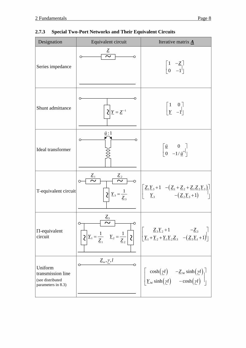
2.7.3 Special Two-Port Networks and Their Equivalent Circuits
Designation Equivalent circuit Iterative matrix A
Series impedance
~Z
1
0 1
Z
Shunt admittance ~
1Y Z
1 0
1Y
Ideal transformer
:1ü
*
0
0 1/
ü
ü
T-equivalent circuit
~ ~
~
1Z 2Z
3
3
1Y
Z
1 3 1 2 1 2 3
3 2 3
1
1
Z Y Z Z Z Z Y
Y Z Y
-equivalent
circuit
~
~ ~
3Z
2
2
1Y
Z1
1
1Y
Z
3 2 3
1 2 1 2 3 3 1
1
1
Z Y Z
Y Y Y Y Z Z Y
Uniform
transmission line
(see distributed
parameters in 8.3)
w , ,Z l
W
W
cosh sinh
sinh cosh
l Z l
Y l l

3 Three-Phase System Page 9
3 Three-Phase System
3.1 Wye Connection and Delta Connection
Three-phase system with two loads (wye connection and delta connection)
aZ~ ~ ~bZ cZ
b
c
a
abY
caY
bcY
~~ ~aI bI cI
aU bU cU
aI bI cI
wye connection delta connection
StrU
StrI
Str Str,U I
E, a, b,c
caUbcU
abU
MEME , U IMEZ ~
M
MU
Line current I
Line-to-line voltage U
Line-to-ground voltage U
Line-to-neutral voltage MU
Phase current StrI , StrI
Phase voltage StrU , StrU
Neutral-to-ground voltage MEU
Neutral(-to-ground) current MEI
Wye connection Y
Relation between phase, neutral and line currents and voltages:
a aStrab a aStr
b bStrbc b bStr
c cStrca c cStr
1 1 0 1 1 0
0 1 1 = 0 1 1 and
1 0 1 1 0 1
U U U I I
U U U I I
U U U I I
and Str MEU U U , ME MEMEU Z I and ME StrI I I
for a,b,c
Delta connection ∆
Relation between phase and line currents and voltages:
a abStr ab abStr a
b bcStr bc bcStr b
c caStr ca caStr c
1 0 1 1 1 0
1 1 0 and = 0 1 1
0 1 1 1 0 1
I I U U U
I I U U U
I I U U U
3 Three-Phase System Page 10
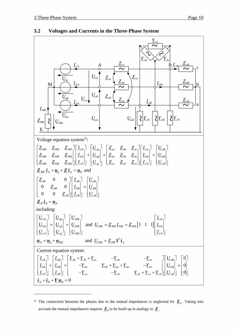
3.2 Voltages and Currents in the Three-Phase System
A Bc
E
M b
a
~
~
~~ ~ ~~
aaZ
bbZ
ccZ
abZ
caZbcZbcU
abUcaU
cBI
bBI
aBI
aEY bEY cEYaBUaAUqaU
qbU
qcU
cAI
bAI
aAI
MEUMEZ
~
~
~aBZ
bBZ
cBZ
~ ~~
abY bcY
caY
MEI
Voltage equation system2):
ME ME ME aA aa ab ac aAqa aB
ME ME ME bA ba bb bc bAqb bB
ME ME ME cA ca cb cc cAqc cB
ME A q A B and
Z Z Z I U Z Z Z I U
Z Z Z I U Z Z Z I U
Z Z Z I U Z Z Z I U
Z i u Z i u
aB aB aB
bB bB bB
cB cB cB
B B B
0 0
0 0
0 0
Z I U
Z I U
Z I U
Z i u
including:
aAaA qa ME
ME ME ME bAbA qb ME ME
cAcA qc ME
T
MEA q ME ME A
and 1 1 1
and
U U U I
U U U U Z I Z I
U U U I
U Z
u u u i1
Current equation system:
aE ab ac ab ac
ba bE ba bc bc
ca cb
aA aB aB
bA bB bB
cA cB cE ca cb cB
A B B
0
0
0
0
Y Y Y Y Y
Y Y Y Y Y
I I U
I I U
Y Y YI I UY Y
i i Y u
2) The connection between the phases due to the mutual impedances is neglected for B
Z . Taking into
account the mutual impedances requires B
Z to be build up in analogy to Z .

3 Three-Phase System Page 11
3.3 Balanced Three-Phase System
3.3.1 Conditions for a balanced three-phase system
a) Geometric symmetry (symmetrical structure of the network components)
Impedance matrix (see Section 3.2):
aa ab ac s g g
ba bb bc g s g
ca cb cc g g s
Z Z Z Z Z Z
Z Z Z Z Z Z
Z Z Z Z Z Z
Z
including aa bb cc sZ Z Z Z and
ab ba bc cb ac ca gZ Z Z Z Z Z Z
Admittance matrix (see Section 3.2):
aE ab ac ab ac s g g
ba bE ba bc bc g s g
ca cb cE ca cb g g s
Y Y Y Y Y Y Y Y
Y Y Y Y Y Y Y Y
Y Y Y Y Y Y Y Y
Y including
aE bE cE EY Y Y Y , ab ba bc cb ac ca gY Y Y Y Y Y Y Y and E s2Y Y Y
b) Electric symmetry (symmetrical (balanced) sources and loads)
Symmetrical sources
Symmetrical loads
2
qa qb qc qa qa qaa a 0U U U U U U
aB bB cB BZ Z Z Z (see footnote 1)
From a) and b) follows: Symmetrical currents and voltages at each location x
2
ax bx cx ax (1 a a) 0I I I I and 2
ax bx cx ax (1 a a) 0U U U U
3.3.2 Single-Phase Equivalent Circuit
Assuming a balanced three-phase system as described in 3.3.1, the general voltage and
current equation systems from 3.2 can be transferred to decoupled equation systems:
s g aA B aBqa aB
s g bA B bBqb bB
s g cA B cBqc cB
0 0 0 0
0 0 0 0
0 0 0 0
U Z Z I U Z I
U Z Z I U Z I
U Z Z I U Z I
and
aA aB s g aB
bA bB s g bB
cA cB s g cB
0 0 0
0 0 0
0 0 0
I I Y Y U
I I Y Y U
I I Y Y U
with MEME
A q
0 and 0
as well as
U I
u u
Single-phase equivalent circuit for the reference phase a of the balanced three-phase
system from Section 3.2
With:
1 s g
1 s g E
q qa
,
3 ,
and
Z Z Z
Y Y Y Y Y
U U
(The index a can be omitted)
B
~
~
1 s gZ Z Z
qU
AI
BU BZ
BIA
AU
~
1 s gY Y Y
The single-phase equivalent circuit for the line a of the balanced three-phase system is
identical to the positive-sequence equivalent circuit (index 1) (see Section 3.5.2).

3 Three-Phase System Page 12
3.3.3 Relations Between Phase, Neutral and Line Voltages and Currents
Wye connection Y
Relation between phase, neutral and line currents and voltages:
a aStrab aStr aStrπ
j2 6
b bStrbc bStr bStr
c cStrca cStr cStr
1 a 3 e and
U U U I I
U U U I I
U U U I I
and Str MU U U
cStrU
bStrU
aStrU
caU
abU
bcU
bStrU
aStrU cStrU
Str
a, b, c
I I
caUabU
bcU bStrU
aStrU
cStrU
Delta connection ∆
Relation between phase and line currents and voltages:
a abStr abStr ab abStr aπ π
j j6 6
b bcStr bcStr bc bcStr b
c caStr caStr ca caStr c
= 1 a = 3 e and = 3 e
I I I U U U
I I I U U U
I I I U U U
cI
bI
aI
caStrI
abStrI
bcStrI
abStrI
caStrI
bcStrI
Str
, a, b, c
U U
cI
bIaI
caStrI
abStrI
bcStrI

3 Three-Phase System Page 13
3.3.4 Phasor Diagram and Three-Phase Apparent Power
aS
aU
aI
a
bS
cS
P
cI
bU
cU
b
c
a3S SQ
bI
Im
Re
a b c
Three-phase apparent power
a b ca b c a b c
j
a a
j
3 e j cos( ) j sin( )
e
S S S S U I U I U I
U I P Q S S
S
3.4 Wye-Delta Transformation
Transformations between delta and wye connections3)
Wye-delta transformation
(Y∆)
a b
ab
Y YY
Y
, b c
bc
Y YY
Y
, c a
ca
Y YY
Y
including a b cY Y Y Y
Delta-wye transformation
(∆Y)
ab caa
Z ZZ
Z
, ab bcb
Z ZZ
Z
, ac bcc
Z ZZ
Z
including ab bc caZ Z Z Z
Transformation for the balanced three-phase system (see Section 3.3)
Y resp. Y Y Z Z
with , a,b,c
Y
3
YY for Y∆ and
3
ZZ
for ∆Y
3) Requirement: No grounding of the neutral point of the wye circuit (ME
0Y resp. ME
Z ).

3 Three-Phase System Page 14
3.5 Unbalanced Three-Phase System
3.5.1 Symmetrical Components
Symmetrical components (SC) of
an unbalanced three-phase system
120°
120° 120° 120°
c1G
b1G
a1Gb2G
c2G
a2G c0Gb0Ga0G
positive sequence (1) negative sequence (2) zero sequence (0)
Phase a as reference phase
a1 1 a2 2 a0 0
2
b1 1 b2 2 b0 0
2
c1 1 c2 2 c0 0
a a
a a
G G G G G G
G G G G G G
G G G G G G
Decomposition of quantities into
symmetrical components
a a1 a2 a0
b b1 b2 b0
c c1 c2 c0
G G G G
G G G G
G G G G
g
Transformation from phase quanti-
ties a, b, c to symmetrical compo-
nents 1, 2, 0 and its inverse trans-
formation
a 1
2
b 2 S S
2c 0
2
1 a
122 bS S
0 c
1 1 1
a a 1
a a 1
1 a a1
1 a a3
1 1 1
G G
G G
G G
G G
G G
G G
g T g
g T g
Phasor diagram of unbalanced
phase quantities and their composi-
tion in symmetrical components
b1G
a2G
a0G
aG
cG
bG
a1G
c1G
b0G
b2G
c2G
c0G
Apparent power in
symmetrical components 1 1
T * * * *
S S 2 2 0 0SS U I U I U I u i
Apparent power in
phase quantities a a
T * * * *
b b c cS U I U I U I u i
Transformation to symmetrical
components is variant in terms of
apparent power
T * T * T T * *
S S S S S S S S
T *
S S S
( ) ( )
3 3
S
S
u i T u T i u T T i
u i

3 Three-Phase System Page 15
3.5.2 Equivalent Circuits in Symmetrical Components
Voltage equations from 3.2 in symmetrical components (decoupled):
1A 1 1A 1B 1Bq1 1B
2A 2 2A 2B 2B2B
ME 0A 0 0A 0B 0B0B
0 0 0
0 0 0 0
3 0 0 0
I U Z I U Z I
I Z I U Z I
Z I Z I U Z I
Current equations from 3.2 in symmetrical components (decoupled):
1A 1B 1 1B
2A 2B 2 2B
0A 0B 0 0B
0
0
0
I I Y U
I I Y U
I I Y U
with 1A q1
2A
ME 0A0A
0
0 0
0 3
U U
U
U Z I
Positive-sequence equivalent circuit:
1 s g
1B B
1 s g E
q1 qa q
3
Z Z Z
Z Z
Y Y Y Y Y
U U U
(compare to single-phase equivalent circuit
of the symmetrical 3-phase system in 3.3.1)
01
A B~
~
1 s gZ Z Z 1AI 1BI
1AU 1BU BZ
~
1 s gY Y Y qU
Negative-sequence equivalent
circuit:
2 1 s g
2B 1B B
2 1 s g E 3
Z Z Z Z
Z Z Z
Y Y Y Y Y Y
02
A B~
~
2 s gZ Z Z 2AI 2BI
2AU 2BU BZ
~
2 s gY Y Y
Zero-sequence equivalent circuit:
0 s g
0B B
0 s g E
2
2
Z Z Z
Z Z
Y Y Y Y
00
A B~
~
0 s g2Z Z Z 0AI 0BI
0AU 0BU BZ
~
0 s g2Y Y Y
~
ME3Z
MEU
The neutral-to-ground impedance MEZ affects only the zero-sequence system. The
neutral-to-ground voltage is: ME 0AME 3U Z I
For the balanced three-phase system, the following applies:
The component systems are decoupled and the negative- and zero-sequence equivalent
circuits are passive networks. Thus, the balanced three-system can be described by the
positive-sequence equivalent circuit (see 3.3.1).
For the unbalanced three-phase system, the following applies:
As a result of unbalanced faults, the equivalent circuits of the symmetrical components
are coupled at the fault location (see 3.5.3) The structure of coupling follows from three
fault conditions, which have to be transferred to symmetrical components.

3 Three-Phase System Page 16
3.5.3 Fault Conditions and Interconnections of Equivalent Circuits in Symmet-
rical Components
Fault
type
Fault conditions Intercon-
nection of
the SC Three-phase system Symmetrical components (SC)
abc
E
a b
b c
0
0
U U
U U
a b c 0I I I
1
2
0
0
U
U
0 0I
00
02
01
abc
E
a
b
c
0
0
0
U
U
U
1
2
0
0
0
0
U
U
U
00
02
01
abc
E
a 0U
b
c
0
0
I
I
1 2 0 0U U U
2 1
0 2
I I
I I
00
02
01
abc
E b c 0U U
a
b c
0
0
I
I I
2 1U U
1 2
0
0
0
I I
I
00
02
01
abc
E
b
c
0
0
U
U
a 0I
2 1
0 2
U U
U U
1 2 0 0I I I
00
02
01
abc
E
a
b
c
0
0
0
I
I
I
1
2
0
0
0
0
I
I
I
00
02
01
abc
E
a 0U
b
c
0
0
I
I
1 2 0 0U U U
2 1
0 2
I I
I I
00
02
01
abc
E
b
c
0
0
U
U
a 0I
2 1
0 2
U U
U U
1 2 0 0I I I
00
02
01

4 Equivalent Networks Page 17
4 Equivalent Networks
Positive-sequence equivalent circuit
Internal grid impedance:
1 1N N NjZ Z R X
01
NR1I
1U1NU
internal
grid bus
NjX
1NZ
Positive-sequence impedance
(see Section 12.3 for voltage factor
max 1,1c c )
22
nN nN N1N 1N
k Nk
13
cU cU rZ X
S xI
R-X ratio: N
N N
N
/R
r xX
Three-phase short-circuit power
(fictitious calculation value, see Sec-
tion 12.3 for voltage factor max 1,1c c )
2
nN nNk nN k nN
1N1N
3 33
cU cUS U I U
ZZ
Negative-sequence equivalent circuit
Usually, the negative-sequence im-
pedance for equivalent circuits is:
2 2N 1NZ Z Z
02
2NZ2I
2U
~
Zero-sequence equivalent circuit
The zero-sequence impedance
0 0N ME3Z Z Z
depends on the neutral grounding:
0 k
1N k1
3 2Z I
Z I
( k k1I I three-phase to single-phase short-
circuit ratio) 00
0NZ0I
0U
~
~
ME3Z
For isolated-neutral and resonant-grounded power systems, the following ap-
plies: 0 1NZ Z
For solidly grounded ( ME 0Z ) power systems, the following applies: 0 0N 1NZ Z Z
Special case: stiff network
kS and 1N 2N 0N ME 0Z Z Z Z

5 Synchronous Machines Page 18
5 Synchronous Machines
5.1 Equivalent Circuits for Steady-State Operating Conditions
Positive-sequence equivalent circuit
General generator equation
11 pa 1
1d 1qd 1 q 1
j
j j
U R X I U U
U X X I X X I
Positive-sequence equivalent circuit of salient-pole machines
Salient-pole machine: d qX X
Appropriate: 1 qX X
Positive-sequence impedance:
1 1G a 1jZ Z R X
qjXaR
U
pU1U
1I
QU
01
1GZ
Positive-sequence equivalent circuit of nonsalient-pole machines (or cylindrical-rotor
machines)
Nonsalient-pole machine: d qX X
Appropriate: 1 dX X
Positive-sequence impedance:
1 1G a 1jZ Z R X
djX aR
pU1U
1I
01
1GZ
Synchronous generated voltage (nonlin-
ear function of the excitation current,
no-load characteristic) and field ratio
p fU f I and p
rG 3
U
U
No-load excitation current f0I p f0 rG 3U I U and 1
Over- or underexcitation f f0I I and 1 resp. f f0I I and 1
Rotor displacement angle p p 1 Up U1,U U
Reference impedance
2
rG rGB
rGrG3
U UZ
SI
Armature resistance a a BR r Z
Direct-axis synchronous reactance d d BX x Z
Quadrature-axis synchronous reactance q q BX x Z

5 Synchronous Machines Page 19
Negative-sequence equivalent circuit
Negative-sequence impedance:
2 2G a d q
2 2 2
f f D D Q Q
j( )
2
1( )
4
Z Z R X X
k R k R k R
2GZ
2U
2I
~
02
Zero-sequence equivalent circuit
Zero-sequence impedance:
0 0G ME
a 0G ME ME
3
j 3 3j
Z Z Z
R X R X
0GZ
0U
0I
~
00
~
ME3Z
Typically, the neutral points of synchronous machines are not grounded: MEZ
5.2 Equivalent Circuit for Transient Operating Conditions
Positive-sequence equivalent circuit of nonsalient-pole machines
Direct-axis transient reactance:
d d BX x Z
Transient voltage:
1 1 a d 1
1 1G 1
(0 ) ( j ) (0 )
(0 ) (0 )
U U R X I
U Z I
djX
1U
1I
1U
aR
01
1GZ
The transient voltage 1U (and the subtransient voltage 1U in Section 5.3) are deter-
mined using the terminal voltage and current immediately before ( 0t ) the fault
5.3 Equivalent Circuit for Subtransient Operating Conditions
Positive-sequence equivalent circuit of nonsalient-pole machines
Direct-axis subtransient reactance:
d d BX x Z
Subtransient voltage:
1 1 a d 1
1 1G 1
(0 ) ( j ) (0 )
(0 ) (0 )
U U R X I
U Z I
djX
1U
1I
1U
aR
01
1GZ

5 Synchronous Machines Page 20
5.4 Synchronous Grid Operation
Example: Synchronous machine supplies power to a grid via a transformer and a line
Positive-sequence equivalent circuit (converted to the same voltage level):
pUNU
djX TjX LjX NjX
VjX
NIGI
GU
with the synchronous generated voltage Upj
p p eU U
and the internal grid volt-
age4) UNj
N N eU U
Apparent power supplied to the
internal bus of the grid5)
pN
pN
*
N N N N N
2jp N N
d V d V
j
C C
j 3
3 3j e j
j e j
S P Q U I
U U U
X X X X
Q Q
Maximum active power supplied to
the internal bus of the grid
p N
kipp
d V
3U U
PX X
Maximum reactive power supplied
at the internal bus of the grid
for 0
2
NC
d V
3U
QX X
Resulting rotor displacement an-
gle4)
(Reference: internal grid voltage)
pN p N Up UN,U U
Resulting field ratio4)
(Reference: internal grid voltage)
p
N
U
U
4) The internal grid voltage UN is a stiff voltage which describes the power exchange within the network
and to which the resulting values of the rotor displacement angle and the field ratio are referenced. For
XV = 0, the equations for these variables result in the equations in Section 5.1.
5) In order to avoid negative values for the active and reactive powers occurring during normal operating
conditions of synchronous generators when using the PSC, the active and reactive powers consumed at
the internal bus of the grid are considered.

5 Synchronous Machines Page 21
5.4.1 Power to Load Angle Characteristics
Active power to load angle characteristic Reactive power to load angle characteristic
N kipp pNsinP P N C pNcos 1Q Q
NP
kipp(1,5)P
kipp(1,0)P 1
1,5
π / 2 π pN
NQ
CQ
pN
1
2
3
π / 2 π
0
5.4.2 Power Diagram
pN
NP
NS
max
TmaxPG GmaxI I
CQpN π / 2
N 0Q
N 0Q
QN
Stability reserve
Valid operating area
NQ
1 0
pNj
Cj eQ
inductive operation
“overexcited operation“
Reactive power is
supplied to the grid.
capacitive operation
„underexcited operation“
Reactive power is
supplied from the grid.
PN
maximum
turbine power
In practice, the operating ranges inductive and capacitive operation are also referred to
as "overexcited operation" and "underexcited operation", although, depending on the
current delivered to the grid, capacitive operation with N 0Q is also possible in over-
excited operation of the synchronous machine with f f0I I .

5 Synchronous Machines Page 22
5.5 Principle of Angular Momentum and Equations of Motion
Synchronous speed 0 0
02π 2π
fn
p p
Number of pole pairs p
Mechanical and electrical
angular velocity 2πn and 2πp np
Principle of angular momentum T DJ M M M
Moment of inertia rotor turbine(s)J J J
Relation between power,
torque and speed
0
02πΩ Ω
P M n M
Equation of motion
(for 0 )
M T N D
M T N M
( )
( )
k P P P
k P P d
and
0 0
Damping power D 0( )P D D D
Damping constant D
Machine constants 0
M
M rG
kT S
and M Md D k
Electromechanical time constant
2
0M
rG
JT
S
Relation between angular coordi-
nates 0 0t
0
0q-axis
synchronous rotating
reference system
(stationary phasor)
coordinate system of the stator
(e.g. firmly fixed to phase a)
d-axis

6 Induction Machines with Squirrel-Cage Rotor Page 23
6 Induction Machines with Squirrel-Cage Rotor
6.1 Simplified Equivalent Circuits for Steady-State Operating Conditions
Positive-sequence equivalent circuit (assumption hX )
01
1I
1U
σs σL kj jX X X
LR
s
SR
01
1I
1UL
1 sR
s
k L SR R R kjX
Components of equivalent circuits
(rotor quantities converted to stator side)
SR Stator resistance
σSX Stator leakage reactance
LR Rotor resistance
σLX Rotor leakage reactance
Splitting L /R s into slip-dependent and slip-independent parts results in the equivalent
circuit on the right side. The stator resistance SR is negligible for motors in the medium-
and high-power range at nominal frequency.
Slip and synchronous rotational
speed 0
0
n ns
n
with 0
02π
fn
p p
Positive-sequence impedance: L L1 1M S σS σL kj( ) j
R RZ Z R X X X
s s
Rated apparent power r mech
rM
rM rMcos( )
PS
(motor operation)
Short-circuit impedance with
starting current anI measured when
starting with rMU and 1s
2
rM1M B
an rM rM an rM
2 2 2 2
S L k L k
1 1
( )
UZ Z
I I S I I
R R X R X
Losses at rated current and 1s 2 2 rMVkr S L rM L rM L
B
3 3S
P R R I R I RZ
Negative-sequence equivalent circuit (assumption hX )
Negative-sequence impedance
L2 2M S kj
2
RZ Z R X
s
with
0 0 02
0 0
2 ( )2
n n n n ns s
n n
02
2I
2U
L SR R kjX
2L
2
1 sR
s

6 Induction Machines with Squirrel-Cage Rotor Page 24
Zero-sequence equivalent circuit (assumption hX )
Zero-sequence impedance
0 0M ME
L S 0k ME ME
3
j 3 j3
Z Z Z
R R X R X
with 0k k X X
00
0I
0U
~0MZ
~
ME3Z
Typically, the neutral points of induction machines are not grounded: MEZ
6.2 Simplified Equivalent Circuits for Transient Operating Conditions
Positive-sequence equivalent circuit (assumption hX )
Transient motor impedance:
1M S k kj jZ R X X
Transient voltage:
M 1 S k 1
1 1M 1
(0 ) j (0 )
(0 ) (0 )
U U R X I
U Z I
01
1U
1ISR kjX
1MZ MU
The transient voltage MU is determined using the values of the terminal voltage and
current immediately before ( 0t ) the fault (e.g. short-circuit).
6.3 Equation of Motion
Equation of motion (Angular momentum theorem) M m wJ M M
Resistive torque
2
w w0 w1 w2 2
0 0
M M M M
Rotational speed and mechanical
angular velocity
(L
f = rotor frequency)
0 L 0 0(1 )(1 )
2π 2π 2π
f f sn s
p p
Torque (Kloss’s equation)
kipp
kipp 2 2
kipp
2s sM M
s s
Breakdown torque and slip
2
1kipp
0 k
13
2π 2
UM
n X and L
kipp
k
Rs
X

7 Transformers Page 25
7 Transformers
7.1 Vector Group Symbols
Winding connection Symbol HV code letter MV/LV code letter
Wye connection Y y
Delta connection D d
Zigzag connection Z z
Grounding available YN, ZN yn, zn
Autotransformer Ya / Yauto
Vector group symbols of two-winding transformers
= HV letter LV letter vector group covector gr de numboup er k
Vector group symbols of three-winding transformers
HV-MV
HV-LV
= HV letter MV letter vector group code number
LV letter vector group code number
vector group
k
k
The vector group code number k indicates the multiple of 30° by which the phasors
of the phase voltages of the MV and LV winding lag behind those of the HV winding
in symmetrical steady-state operation.
7.2 Conversions of Variables Between Transformer Voltage Levels
Transformation ratios (HV, MV and LV)
Positive-sequence system
π πj j
rTHV HV6 61 SG
rTLV LV
e ek kU w
ü ü mU w
Negative-sequence system *
2 1ü ü
Zero-sequence system 0 10ü ü ü ü
Conversion of pos.-seq. variables LV to HV HV to LV
Voltage 1LV 1 1LVU ü U 1HV 1HV
1
1U U
ü
Current 1LV 1LV*
1
1I I
ü *
1HV 1 1HVI ü I
Impedance 2
1LV 1 1LVZ ü Z 1HV 1HV2
1
1Z Z
ü
Corresponding conversions of negative- and zero-sequence variables are carried out
analogously using the respective transformation ratios.
7 Transformers Page 26
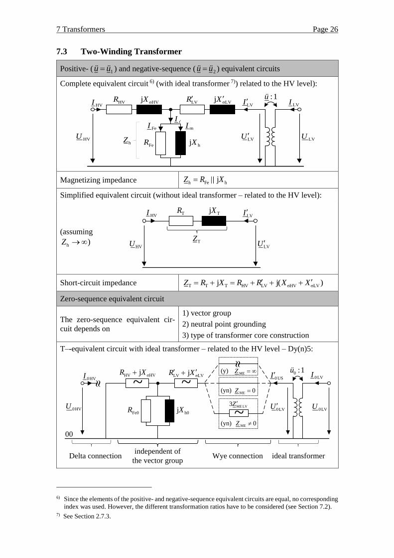
7.3 Two-Winding Transformer
Positive- ( 1ü ü ) and negative-sequence ( 2ü ü ) equivalent circuits
Complete equivalent circuit 6) (with ideal transformer 7)) related to the HV level):
HVR σHVjX LVR σLVjX
FeR hjXHVU LVULVU
LVI HVI LVI
mI
:1ü
FeI
hZ
I
Magnetizing impedance h Fe hjZ R X
Simplified equivalent circuit (without ideal transformer – related to the HV level):
(assuming
h )Z
TR TjX
HVU LVU
LVI HVI
TZ
Short-circuit impedance T T T HV LV σHV σLVj j( )Z R X R R X X
Zero-sequence equivalent circuit
The zero-sequence equivalent cir-
cuit depends on
1) vector group
2) neutral point grounding
3) type of transformer core construction
T–-equivalent circuit with ideal transformer – related to the HV level – Dy(n)5:
HV σHVjR XLV σLVjR X
h0jX0HVU0LVU
0HVI 0 USI 0LVI
0LVU
Delta connectionindependent of
the vector group
0 :1ü
Wye connection
ME 0Z (yn)
ME LV3Z
ME 0Z (yn)
(y)
ideal transformer
~ ~
~
MEZ
00
Fe0R
6) Since the elements of the positive- and negative-sequence equivalent circuits are equal, no corresponding
index was used. However, the different transformation ratios have to be considered (see Section 7.2). 7) See Section 2.7.3.

7 Transformers Page 27
7.4 Calculation of the Transformer Equivalent Circuit Elements
7.4.1 Calculation of the Series Impedance Using the Short-Circuit Test
The magnetizing impedance can be neglected while calculating the series impedance.
Reference impedance
2
rTB
rT
UZ
S
rT rTHVU U for the HV level
rT rTLVU U for the LV level
Short-circuit impedance 2
rTT k k B
rT
UZ u u Z
S
Resistance of the short-circuit im-
pedance
2
Vkr VkrrTT T B T B R B2
rT rT rT3
P PUR r Z r Z u Z
S I S
Reactance of the short-circuit im-
pedance 2 2 2 2
T T T k R B X BX Z R u u Z u Z
Generally, RT and XT are equally divided between the HV and LV winding impedances8)
of the positive-, negative- and zero-sequence equivalent circuits, see section 7.3.
7.4.2 Calculation of the Magnetizing Impedance by an Open-Circuit Test
The series impedance can be neglected for the calculation of the magnetizing imped-
ance.
Open-circuit current rT
h3
UI
Z
2
rTB
h rT h
1 1Ui Z
Z S Z
Magnetizing current rTm
h3
UI
X
2
rTm B
h rT h
1 1Ui Z
X S X
Open-circuit impedance
2
rTh B
rT
1 1UZ Z
i S i
Iron loss resistance
2
rTFe B
V r V r rT
1
/
UR Z
P P S
Magnetizing reactance m m
2
h Fe rTh B
2 2rTFe h
1 1Z R UX Z
i S iR Z
Zero-sequence magnetizing reactance h0 0 h1X k X ( 0k dependent on core construction)
The elements of the zero-sequence equivalent circuit can either be determined by an addi-
tional open-circuit test by feeding into a zero-sequence system or in a simplified manner by
using a factor 0k to estimate the elements.
8) The impedance is specified as impedance per phase for the three-phase transformers. Exemplarily, the
impedances of delta-connected windings are converted to an equivalent representation of wye-connected
windings.
7 Transformers Page 28
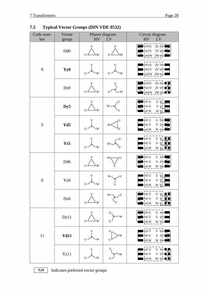
7.5 Typical Vector Groups (DIN VDE 0532)
Code num-
ber
Vector
group
Phasor diagram
HV LV
Circuit diagram
HV LV
0
Dd0 V
U W
V
U W 1W
1V
1U
2W
2V
2U
Yy0
V
U W
V
U W 1W
1V
1U
2W
2V
2U
Dz0 V
U W
V
U W 1W
1V
1U
2W
2V
2U
5
Dy5
V
U W V
U
W
W
V
U
W
V
U
Yd5
V
U W V
U
W
W
V
U
W
V
U
Yz5
V
U W V
U
W
W
V
U
W
V
U
6
Dd6 V
U W V
UW
W
V
U
W
V
U
Yy6 V
U W V
UW
W
V
U
W
V
U
Dz6 V
U W V
UW
W
V
U
W
V
U
11
Dy11 V
U W
V
U
W
W
V
U
W
V
U
Yd11
V
U W
V
U
W
W
V
U
W
V
U
Yz11
V
U W
V
U
W
W
V
U
W
V
U
Yy0 Indicates preferred vector groups

7 Transformers Page 29
7.6 Three-Winding Transformer
Positive- and negative-sequence equivalent circuits
Simplified equivalent circuit (without an ideal transformer, related to the HV level):
HVZ MVZ
HVU
HVI
LVI
MVI
LVZ
MVU LVU
~ ~
~
FeR hjX
The calculation of the equivalent circuit parameters of a three-winding transformer is
subject to the same calculation specifications as for the two-winding transformer. A
minimum of three short-circuit tests is required to calculate the three series impedances.
The magnetizing impedance ( hX and FeR ) is calculated according to Section 7.4.2 us-
ing the data of the open-circuit test.
Maximum power transport between
windings
rTHVMV rTHV rTMVmin ,S S S
rTHVLV rTHV rTLVmin ,S S S
rTMVLV rTMV rTLVmin ,S S S
Short-circuit impedances related to
the HV level
2
rTHVHVMV kHVMV
rTHVMV
UZ u
S
2
rTHVHVLV kHVLV
rTHVLV
UZ u
S
2
rTHVMVLV kMVLV
rTMVLV
UZ u
S
Winding impedances 9)
HV HVMV
HVLVMV
MVLVLV
1 1 11
1 1 12
1 1 1
Z Z
Z Z
Z Z
9) The values of the winding impedances can partly become negative. This is due to the structure of the
equivalent circuit used.

8 Transmission Lines Page 30
8 Transmission Lines
The equations for the line constants and the positive-, negative- and zero-sequence
equivalent circuits are identical with regard to the structure. By means of the respective
primary line parameters per unit length for the positive-, negative- and zero-sequence
system, the line constants are calculated and the elements of the equivalent circuits are
parameterized.
8.1 Surge Impedance and Propagation Constant
Transmission lines (affected by losses)
Characteristic impedance
(surge impedance) w
w
j 1
j
R LZ
G C Y
Propagation constant with attenuation con-
stant and phase(change) constant j j jR L G C
, , andR L G C are the primary line parameters per unit length in
/ km, H / km, S / km and F / km
Low-loss transmission lines ( R L and G C )
Characteristic impedance10) and character-
istic admittance w
w
1 11 j
2
L R LZ
Y C L C
Propagation constant with attenuation con-
stant and phase(change) constant
1j
2
R GL C L C
L C
8.2 Solution of the Line Equations in the Frequency Domain
Voltage and current at the location x along the line (node A: x = 0, node B: x = l)
depending on the terminal values at node A:
wA
Aw
cosh sinh( )
( ) sinh cosh
x Z xU x U
I x IY x x
depending on the terminal values at node B:
wB
Bw
cosh sinh( )
( ) sinh cosh
l x Z l xU x U
I x IY l x l x
10) The capacitive component of the characteristic impedance (imaginary part) can usually be neglected for
low-loss lines due to its small size.

8 Transmission Lines Page 31
8.3 Distributed Line Model and Two-Port Equations
Equivalent circuit with distributed parameters
w
sinh
Z
l
AI BI
AU BU
w
cosh 1
sinh
lZ
l
~
~ ~
T–equivalent circuit
w
sinh
Y
lAI BI
AU BU w
cosh 1
sinh
lY
l
~~~
–equivalent circuit
Two-port equations
Impedance representation
w w
AA
BB
w w
cosh 1
sinh sinh
cosh1
sinh sinh
lZ Z
l lU I
U IlZ Z
l l
Admittance representation
w w
A A
B B
w w
cosh 1
sinh sinh
cosh1
sinh sinh
lY Y
l l UI
UI lY Y
l l
Iterative representation (cascade or
transmission representation)
wA B
A Bw
cosh sinh
sinh cosh
l Z lU U
I IY l l
8.4 Approximations for Electrically Short Transmission Lines ( 1l )
Equivalent circuit with lumped parameters
L LjG C
AI BI
AU BU
L L
1j
2R X
~
~ ~
L LjR XAI BI
AU BULj
2
C
~L
2
GCAI
L
2
GCBI
λI
T– equivalent circuit – equivalent circuit
Equivalent circuit elements (Line length l) LR R l , LL L l , LC C l , LG G l
See Section 2.7.2 for two-port equations of T– and –equivalent circuit

8 Transmission Lines Page 32
8.5 Operational Performance
Voltage drop Z A BU U U
Voltage difference A BU U U
Transmission angle AB A B
Capacitive charging current11) B
LC A CA CB A B0
j2I
CI I I I U U
Capacitive charging power12) * 2
CC A L nNIm 3Q U I C U
8.6 Terminal Power, Losses and Reactive Power Demand
Power at the line terminals (see two-
port network in 2.7.2)
* 2 * *
AA A AB A BA A A
* 2 * *
BB B BA B AB B B
j3
j
Y U Y U US P Q
Y U Y U US P Q
Transmissible active power
(for electrically short lines with neglect of
, and R G C )
A BA B AB AB
L
3 sinU U
P P PX
Line losses VP and
reactive power demand VQ V V V A BjS P Q S S
Line losses (example of Π-equivalent circuit with
lumped parameters) 2 2 2
V L λ L A B A B
13 3
2P R I G U U P P
Reactive power demand (example of Π-equivalent circuit with
lumped parameters) 2 2 2
V L λ L A B A B
13 3
2Q L I C U U Q Q
8.7 Surge Impedance Loading (Natural Load)
Surge impedance loading (SIL)
Condition for
surge impedance loading B w B w BZ Z U Z I
(Termination at node B with characteristic impedance)
Natural load12)
2 2
B BNat Nat*
ww
3 3U U
S PZZ
(apparent power output at terminal B)
Above natural load11) V 0Q for B NatP P resp. B wZ Z
Below natural load11) V 0Q for B NatP P resp. B wZ Z
11) Approximation applies to Π-equivalent circuit with lumped parameters. 12) Approximation applies to low-loss lines (see Section 8.1)

9 Medium- and Low-Voltage Grids Page 33
9 Medium- and Low-Voltage Grids
9.1 Current Distribution
General equivalent circuit: Applies only to voltage-independent load currents
1Z 2Z
AU
1I 2I mIAI1mZ
BU
BI
case a) additionally for case b)
1U 2U mU1M
mZ1mI
1mU
1ZU2ZU
mZU1mZU
Case a) Single-fed line: AU given, without 1mZ
Kirchhoff’s voltage
law provides m
independent
equations
1 1 21 A
2 22 1
B
A
1
2
m
m
m mi
U U Z I I I
I
U U Z I I
U U Z I m
Case b1) Double-fed line: A BU U
General mesh A – B
1
1 1 2 BA B
1
2 2 B 1 B ...
i
m
Z
i
m
U U U Z I I I
Z I I Z I
Calculation of one ter-
minal current using
”torque approach“
(for node B or A)
1 1 1 2 2 1 2B
1 2 1
( ) ( )m m
m
Z I Z Z I Z Z Z II
Z Z Z
Stepwise determination of the current distribution
Case b2) Double-fed line: A BU U
General approach
1.) Calculation of a preliminary current distribution
with A BU U corresponding to case b1
2.) Superposition with an offset current A B
AB 1
1
m
ii
U UI
Z
The current distribution can be used to determine the voltage drops iZU .
9.2 Load Application Factor ε
Conversion of a uniformly distributed load into a concentrated load
l
homogeneous load aggregated load
l l
1U 1U2U 2U
1I 2I nI1
n
i
i
I
1 2 nI I I
1
2
nε
n

10 Rotor Angle Stability of the Single-Machine Problem Page 34
10 Rotor Angle Stability of the Single-Machine Problem
Generator Transformer Line GridTP NPGP
10.1 Small-Signal Stability
Equation of motion (see 5.5) M T N( )k P P and 0 0
Operating point
with turbine power TP
(losses are neglected)
P
TP
π / 2 πpN
Stability reserve
NP
Requirement for small-signal sta-
bility
N
pN
d0
d
P
resp. pN
π π
2 2
Synchronizing power N
s kipp pN
pN
dcos
d
PP P
10.2 Transient Stability
Operating points
with turbine power TP
(losses are neglected)
Applies to transient quantities:
U UN
and (transient voltage U see 5.2)
a NN
d V
3 sinU U
PX X
P
TP
BF
0 a a( )t grenz max
VF
0
NP a
NP
(index 0: before fault, index a: after fault clearance)
Requirement for transient stability V BF F (Law of equal areas)
Law of equal areas
maximum fault clearance time
max grenz
a max
a
Vmax B T kipp( sin )dF F P P
Maximum fault clearance time a max 0a max
M T
2t
k P

11 Line Frequency Control Page 35
11 Line Frequency Control
11.1 Balance Model of the Power System
Differential equation for the calcu-
lation of the line frequency at
T0 L0P P N T Lx TP TS Lstat x
0
fM P P P P P P
f
Turbine and load power
at the operating point T0P and L0P
Inertia constant
of the power system N G G M MM P T P T
Total rated active power of syn-
chronous generators in operation
G
G rG
1
m
i
i
P P
Total rated active power of induc-
tion motors in operation
M
M rM
1
m
i
i
P P
Equivalent generator time constant G
2
G G 0
1G
1m
i
i
T JP
Equivalent motor time constant M
2
M M 0
1M
1 m
i
i
T JP
11.2 Proportional Gains and Droops
Frequency bias of primary control
(absolute and per unit value) and
control droop of the generator i
TP
ii
Pk
f
, 0
P P
rG
i i
i
fk k
P and
rGP
P P 0
1 1 ii
i i
Ps
k k f
Total frequency bias of primary
control and total control droop of
generators
G G
rGP P
1 10 P
1m m
ii
i i i
Pk k
f s
and
G1
rG GP G
1 P P 0
1m
i
i i
P Ps P
s k f
Frequency bias (absolute and per
unit value) and droop of the load i Lik , 0
L L
L0
i i
i
fk k
P and L0
L
L L 0
1 1 ii
i i
Ps
k k f
Total load frequency bias and total
load droop
L
LstatL L
1AP
d
d
m
i
i
Pk k
f
and
L1
L0 L0L L0
1 L L 0
1m
i
i i
P Ps P
s k f
Frequency bias of the power system N P Lk k k

11 Line Frequency Control Page 36
11.3 Power System Operating Point after Completion of Primary Control
(without Secondary Control)
GCC
LCC
PPCC
Pf
L0PL0 xP P
0f
f
f
L
1
k
TPP LstatP
Lstat
L
Pf
k
x
N
Pf
k
TP
P
Pf
k
xP
P
Unplanned change of load xP
Steady-state operation (after completion
of primary control) 0f
Primary control power (Power Plant
Characteristic Curve (PPCC)) T TP PP P k f
Frequency-dependent change of load
(Load Characteristic Curve (LCC)) Lstat LP k f
Load change in the perturbed power
system Lx Lstat xP P P
Frequency change in power system
(Grid Characteristic Curve (GCC)) x
N
Pf
k
11.4 Power System Operating Point after Completion of Secondary Con-
trol
LCC
PPCC
L0P L0 xP P
TSP
L
1
k
P
0f
f
Total secondary control power acti-
vation T TS xP P P

12 Short-Circuit Current Calculation Page 37
12 Short-Circuit Current Calculation
12.1 Short-Circuit Current Over Time k
22
I
gi
b2 2I
k2 2 I
switching off at 115 ms
fault occurrence at t = 0 s
pi
thI
kin
kA
i
4
0
near-to-generator short-circuit with voltage equal to zero
uˆcosu t u t
gd d
k k k k k k k2 e e cos 2 cos e
tt t
TT Ti t I I I I I t I
Near-to-generator short-circuit
if one synchronous machine contributes to an initial short-circuit current kG rG
2i i
I I k b kI I I
Far-from-generator short-circuit k b kI I I
12.2 Characteristic Short-Circuit Current Parameters
Initial symmetrical short-circuit current
(rms value of the AC symmetrical component applicable at instant of short-circuit) kI
Transient short-circuit current
(rms value of the AC symmetrical component in transient time domain) kI
Steady-state short-circuit current
(rms value of the short-circuit current after the decay of the transient phenomena) kI
Peak short-circuit current
(maximal possible instantaneous value of the prospective short-circuit current) pi
Symmetrical short-circuit breaking current
(rms value of the AC symmetrical component at the instant of contact separation) bI
Thermal equivalent short-circuit current
(rms value of short-circuit current having the same thermal effect and the same dura-
tion Tk as the decaying short-circuit current) thI
Time constants (sub-transient, transient, direct-current) d d g, ,T T T
Angle of short-circuit impedance kZ at short-circuit location Zk
Initial phase angle of the voltage at short-circuit location u
Initial phase angle of the short-circuit current ki t u Zk

12 Short-Circuit Current Calculation Page 38
12.3 Method of the Equivalent Voltage Source at the Short-Circuit Loca-
tion (According to IEC 60909 and VDE 0102)
Calculation independent of operating point, approximation of the minimal and maximal
absolute value of the initial symmetrical short-circuit current kI 13)
ersU
kI
~kZ
Reverse feeding into the
passive network at the
short-circuit location
Equivalent voltage
source ersU at the short-
circuit location
Neglect of shunt admit-
tances and non-rotating
loads14)
Initial symmetrical short-circuit current ers n
k
k k3
U UI c
Z Z
Equivalent voltage source at the short-circuit location n
ers3
UU c
Voltage factor c for the calculation of the maximum
short-circuit currents15) max 1,1c
Voltage factor c for the calculation of the minimum
short-circuit currents15) min 1,0c
Short-circuit impedance at the short-circuit
location16)
(effective impedance at the instant of the short-circuit)
k k kjZ R X
Peak short-circuit current
(κ: see factor in Section 12.5.1) p k2i I
Symmetrical short-circuit breaking current17)
(µ: see factor in Section 12.5.2) b kI I
Thermal equivalent short-circuit current
(m and n: see factors in Section 12.5.3) th kI m n I
Steady short-circuit current kI
13) For the consideration of the short-circuit current contributions of doubly-fed induction generator-based
wind turbines and power station units with full-size converter see IEC 60909. 14) Deviations are possible for the zero-sequence system. 15) Valid for nominal system voltages > 1 kV 16) For the calculation of the maximum initial symmetrical short-circuit current according to IEC 60909,
impedance correction factors shall be applied in accordance with Section 12.4. 17) Only valid for near-to-generator single-fed three-phase short-circuits.

12 Short-Circuit Current Calculation Page 39
12.4 Consideration of Impedance Correction Factors
(according to IEC 60909 and VDE 0102)
Impedance correction factors for calculating the maximum short-circuit currents18)
The short-circuit impedance Zk at the short-circuit location should be calculated with
corrected impedances. The defined value of the equivalent voltage source at the short-
circuit location is in many cases not sufficient to calculate the initial symmetrical short-
circuit currents and the partial initial short-circuit currents within a fault limit of 5 %.
Therefore, the implementation of impedance correction factors is necessary.
Two-winding transformers19)
TK TTZ K Z
maxT
T
0,951 0,6
cK
x
Three-winding transformers
HVMVK T HVMVT HVMV
HVLVK T HVLVT HVLV
MVLVK T MVLV T MVLV
Z K Z
Z K Z
Z K Z
maxT HVMV
T HVMV
maxT HVLV
T HVLV
maxT MVLV
T MVLV
0,951 0,6
0,951 0,6
0,951 0,6
cK
x
cK
x
cK
x
Synchronous machines20)
GK GGZ K Z
nN maxG
2rG d rG1 1 cos
U cK
U x
Power station units with on-load
tap changer21)
2
SK G T HVSZ K ü Z Z
22rTLVnN max
S 2 2 2rG rTHV d T rG1 1 cos
UU cK
U U x x
Power station units without on-
load tap changer21)
2
SOK G T HVSOZ K ü Z Z
rTLV T maxnNSO
2rG G rTHV d rG
1
1 1 1 cos
U p cUK
U p U x
18) In case of unbalanced short-circuits, the impedance correction factors shall be applied to the negative-
and the zero-sequence system. Impedances between a neutral point and ground shall be introduced with-
out correction factor. 19) cmax is related to the nominal voltage of the network connected to the low-voltage side of the network
transformer. The impedance correction is not valid for unit transformers and wind power station units. 20) Not to be used, if connected via a unit transformer. 21) To be used in case of short-circuits on the high-voltage side of the unit transformer.

12 Short-Circuit Current Calculation Page 40
12.5 Factors for the Calculation of Short-Circuit Currents
12.5.1 Factor κ for the Calculation of the Peak Short-Circuit Current ip
Determination of κ by the methods a), b) and c) according to IEC 60909
Factor for the calculation of the peak short-circuit current22) 31,02 0,98 e R X
a) Uniform ratio R X : The smallest ratio R X of the network branches carrying par-
tial short-circuit currents at the nominal voltage corresponding to the short-circuit
location applies to all short-circuit locations.
b) Ratio R X at the short-circuit location: For the ratio R X , the ratio k kR X of the
short-circuit impedance kZ at the short-circuit location is used: k kR X R X . To
cover inaccuracies within the network reduction to a single short-circuit impedance,
the factor (b) 1,15 is applied, if k k 0,3R X , else (b) .
c) Equivalent frequency cf : Determination of the short-circuit impedance at the short-
circuit location c c cjZ R X for the equivalent frequency c 20 Hzf (at a line
frequency 50 Hzf ). To be applied: c c c /R X R X f f .
12.5.2 Factor µ for the Calculation of the Sym. Breaking Current Ib
0 1 2 3 4 5 6 7 8 9
I''
kG/I
rG
0.5
0.6
0.7
0.8
0.9
1
tmin
0.02 s
0.05 s
0.10 s
0.25 s
Minimum time delay
Minimum time delay:
shortest time between the beginning of the
short-circuit current and the contact separation
of the first pole to open the switching device
Factor µ for the calculation of the symmetrical breaking current in case of a near-to-generator single-fed
three-phase short-circuit
22) For further details and conditions please refer to IEC 60909.

12 Short-Circuit Current Calculation Page 41
12.5.3 Factors m and n for the Calculation of the Thermal Equivalent Short-Cir-
cuit Current Ith
Factor m for the consideration of the heat effect of the DC component of the short-circuit current
Factor n for the consideration of the heat effect of the AC component of the short-circuit current

12 Short-Circuit Current Calculation Page 42
12.6 Calculation with Kirchhoff’s Laws
Calculation depends on operating point, exact calculation of the initial symmetrical
short-circuit current kI by magnitude and phase angle using the superposition method
Calculation of
partial short-circuit currents ers
kG
G
IU
Z
,
NkN
ers N
UI
Z , …
Calculation of the exact
initial symmetrical short-circuit current k kG kN ...I I I
12.7 Thermal Short-Circuit Strength
DC resistance at 20
20 : Specific conductivity at 20 C
l : Conductor length
A : Conductor cross-section
0
20
lR
A
DC resistance at x
20 : Temperature coefficient of re-
sistance at 20 C
0 20 x 201R R
Thermal equivalent short-circuit current k
2
th k k
k 0
1( )d
T
I I m n i t tT
Duration of the short-circuit current (=sum of short-circuit durations in case of suc-
cessive short circuits with short pauses)
k
k k
1
N
i
i
T T
Determination of thermal short-time
strength of electrical machines, trans-
formers, transducers, reactors and
switching devices
th thrI I for k krT T
krth thr
k
IT
IT
for k krT T
Thermal equivalent short-circuit
current density
b : Conductor temperature at the
beginning of a short-circuit
e : Conductor temperature at the end
of a short-circuit
20 p 20 e
20
th k
k 20 b
th
1 20 C ln
1 20 C
I I mS
A A
T
n
c
pc : Specific thermal capacity
: Density of conductor
Rated short-time withstand current density thr thS S calculated with:
b b,max : Maximum permissible operating temperature (unless otherwise known)
e e,max : Maximum permissible temperature in the event of a short-circuit
k krT T : Rated duration of the short-circuit current (e.g. 1 s)

12 Short-Circuit Current Calculation Page 43
Determination of thermal short-time
strength of overhead line conductors,
cables and busbars
krth thr
k
ST
ST
Text Rated short-time withstand current density depending on the conductor tempera-
ture at the beginning of the short-circuit b
and the conductor temperature at the end
of the short-circuit e
for a rated duration of the short-circuit current kr
1sT for alu-
minum, as wells copper and steel
copper
steel

12 Short-Circuit Current Calculation Page 44
12.8 Mechanical Short-Circuit Strength
12.8.1 Determination of Magnetic Fields and Forces
3( )i t1( )i t 2( )i t
x
y
z
l
1( , )B i r
12d 23d
13d
L (conductor radius)ij
l d
d r
2( , )B i r 3( , )B i r
Determination of field quantities
Magnetic flux density 0 rμB H
Magnetic field strength ( , )2π
iH I rr
I
Magnetic force between conductors
(Lorentz force, right-hand rule) ( )F I l B
Determination of magnetic forces (three-phase system)
Absolute value of the magnetic force between two
conductors i and j
0r
μ( ( ) () )
2πij i j
ij
lF it tt i
d

12 Short-Circuit Current Calculation Page 45
12.8.2 Maximum Forces Between Main Conductors and Sub-Conductors
Maximum main conductors force acc. IEC 60865-1 during a 3-phase short-circuit
pi : Peak short-circuit current
l : Center-line distance between supports
ma : Effective distance between main conductors
a : Center-line distance between conductors
20m p
m
μ 3
2π 2
lF i
a
Main conductors consisting of single
circular cross-sections ma a
Main conductors consisting of single rectangular
cross-sections (factor 1sk see figure below) m
1s
aa
k
Maximum sub-conductors force acc. to IEC 60865-1 during a 3-phase short-circuit
n : Number of sub-conductors
sl : Center-line distance between connecting pieces
or between one connecting piece and the adja-
cent support
2
p0 ss
s
μ
2π
i lF
n a
sa : Effective distance be-
tween sub-conductors
Effective distance between sub-conductors with cir-
cular cross-sections 2s 1
1 1n
i ia a
Effective distance between sub-conductors with rec-
tangular cross-sections (factor 1sk see figure below) 1
2s 1
1 ni
i i
k
a a
12a13a
1sa1na
...
...
...
...
...
...
...
...
a
b
d
b
d
12a13a
1sa1na
1
1,2
1,5
2,0
2,6
3,0
3,55
6
8
10
1216
20
4,0
/ 0,1b d
0,4
0,6
0,8
4,5

12 Short-Circuit Current Calculation Page 46
Factor 1s
k for the calculation of the effective conductor distance
12.8.3 Calculation of Mechanical Stress
Bending stress caused by forces
between main conductors m
m σ r8
F lV V
Z
σV : Ratio of dynamic and static main conductor stress
rV : Ratio of dynamic stress with unsuccessful three-phase automatic reclosing and dy-
namic stress with successful three-phase automatic reclosing
Z : Section modulus of main conductor in direction of the bending axis
: Factor for main conductor stress (depends on type of beam and support)
Single-span beam
A and B simple
supports A B 1,0
A: fixed support
B: simple support A B
0,73
A and B fixed
supports A B
0,5
Continuous beam
with equidistant
simple supports
Two spans A B A
0,73
Three or more spans A B B A
0,73
Bending stress caused by the forces
between the sub-conductors s s
s σs rs
s16
F lV V
Z
The variables with the index s are defined analogously to the variables for the main
conductors given above.
A conductor is mechanically short-cir-
cuit-proof, if: tot m s zul p0,2q R
tot : Total conductor stress
p0,2R : Stress corresponding to the yield strength
q : Factor of plasticity (depends on the conductor profile and load)
Section moduli Z are defined with respect to bending axis
rectangle
z
y h
b
circle
z
y
D
circular ring
z
y
Dd

12 Short-Circuit Current Calculation Page 47
2 2
y z,6 6
bh hbZ Z
3
y z
π
32Z Z Z D
4 4
y z
π
32
D dZ Z Z
D

13 Neutral Grounding Page 48
13 Neutral Grounding
13.1 Equivalent Circuit for Single-Phase Line-to-Ground Faults
General equivalent circuit for neutral-point grounding
c
E
Mb
a
qaU
qbU
qcU
cAI
bAI
aAI
MEU
caY
abY
aEY
bcY
aFIMEI
cEYbEY
ME
ME
1Z
Y
aaZ
bbZ
ccZ
abZ
caZbcZ
B
cEIbEIaEI
abI
bcI
caI
aBU
cBI
bBI
aBI
A
CE GEI I
~
~
~
~ ~ ~ ~
~
~
~
Assumption: Balanced three-phase system with , a,b,ci k
E E E EjiY Y G C l , jikY Y G C l
s s sjiiZ Z R X , g g gjikZ Z R X
MEME ME2 2
ME ME ME ME ME ME ME
1 1 1 1j j
j
RY G
Z R L R X X L
13.2 Currents and Voltages at Single-Phase Line-to-Ground Faults
Fault current at single-phase line-to-ground fault q1 qaU U
Fault current at single-phase
line-to-ground fault
( 1F 2FZ Z ) q
aF 1F CE G
1 q1
1F 2F 0F 1
E ME
F
3
33
2
I
U U
Z Z Z m Z
I I I I
Capacitive ground fault cur-
rent bF cF bF cC E FE Ej jU U l U UI C C
Conductive ground fault cur-
rent bF cF FE b FE cG EI UG GU U l U
Neutral-to-ground current ME ME MEI Y U

13 Neutral Grounding Page 49
Line-to-ground voltages of phases without faults
Line-to-ground voltages of
phases without faults
bF b U f m , cF c U f m
2 2
bF q1 q1
a a a 1 3 3 j
2 2 2
m mU U U
m m
2
cF q1 q1
a a a 1 3 3 j
2 2 2
m mU U U
m m
Positive- / negative- / zero-sequence port impedances at short-circuit location
Positive- and negative-
sequence port impedances at
short-circuit location
1F 2F
1 E
1 s g
1 1
1 13
Z Z
Y Y YZ Z Z
Zero-sequence port
impedance at short-
circuit location
0F
0 E
0 ME s g ME
1 1
1 1
3 2 3
Z
Y YZ Z Z Z Z
Factor m
(zero-sequence / positive-sequence
port impedance ratio)
0F0F 1F
1F
for Z
m m Z ZZ
Ground fault factor for pre-fault line-to-line voltage b
q13U U
Ground fault factor for single-
phase line-to-ground faults
2 bF cF
b
max , 1 3
23
m mU U m m
mU
3m
effectively grounded grid
1,4 5,5m
0F 1Fm Z Z
k1
k3
0I
mI
k1
k3
II
low-impedance grounding
solid / partially solid current-limiting
isolated neutral
resonant-grounded

13 Neutral Grounding Page 50
13.3 Isolated Neutral Point
MEZ , 1F 2F 0F E1Z Z Z Y , 1m
Neutral-to-ground voltage ME qa q1U U U
Fault current for single-phase
line-to-ground fault = (nega-
tive) cap. ground fault current CE GE CE E q1aF j3I I I I C U
Line-to-ground voltages of
phases without faults
π
j6
bF q1 q1
3 3 j 3 e
2U U U
π
j6
cF q1 q1
3 3 j 3 e
2U U U
Ground fault factor 3
13.4 Resonant-Grounded Neutral Point (RESPE)
MEZ f v , 1F 2F 0F ME E1 3Z Z Z Y Y , 1m
Neutral-to-ground voltage qa q1MEU U U
Fault current for single-phase
line-to-ground fault = ground
fault current = residual current aF CE GE ME Rw Rb
q1CE
R
E
j
3j j j
I I I I I I
I d v d v
I
C U
Detuning
0 undercompensated
0 overcompensated
v
v
2
E ME
11
3v
C L
Attenuation
ME E
E
3
3
G Gd
C
Line-to-ground voltages of
phases without faults
πj6
bF q1 3 eU U
πj6
cF q1 3 eU U
Ground fault factor 3
Neutral displacement voltage during undisturbed operation without ground fault
Assumption: Unbalanced line-to-ground admittances aE bE cEY Y Y
Neutral-to-ground voltage ME qaj
kU U
d v
Imbalance factor
2
aE bE cE
E3
Y a Y aYk
C
Mean values of line-to-
ground capacitances and con-
ductances E aE bE cE
1
3C C C C , E aE bE cE
1
3G G G G
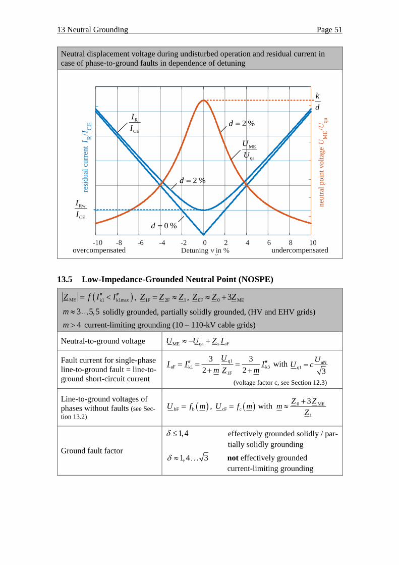
13 Neutral Grounding Page 51
Neutral displacement voltage during undisturbed operation and residual current in
case of phase-to-ground faults in dependence of detuning
-10 -8 -6 -4 -2 0 2 4 6 8 10
Verstimmung v in %
IR
/IC
E
Ver
lage
rungs
spannung
UM
E/U
qa
overcompensated undercompensated
2 %d
0 %d
2 %d
R
CE
I
I
ME
qa
U
U
Rw
CE
I
I
k
d
Detuning in %v
neu
tral
po
int
vo
ltag
eU
ME
/Uqa
resi
du
al c
urr
ent
13.5 Low-Impedance-Grounded Neutral Point (NOSPE)
ME k1 k1maxZ f I I , 1F 2F 1Z Z Z , 0F 0 ME3Z Z Z
3 5,5m solidly grounded, partially solidly grounded, (HV and EHV grids)
4m current-limiting grounding (10 – 110-kV cable grids)
Neutral-to-ground voltage s aFME qaU U Z I
Fault current for single-phase
line-to-ground fault = line-to-
ground short-circuit current
q1
k1 k3
1F
aF
3 3
2 2I
UI I
m Z m
with n
q1N
3
UcU
(voltage factor c, see Section 12.3)
Line-to-ground voltages of
phases without faults (see Sec-
tion 13.2)
bF b U f m , cF c U f m with 0
1
ME3
Z
Z Zm
Ground fault factor
1,4 effectively grounded solidly / par-
tially solidly grounding
1,4 3 not effectively grounded
current-limiting grounding

14 Thermodynamics Page 52
14 Thermodynamics
Heat flow and
quantity of heat
th
th th
d
d
Q tP t Q t
t
Law of conservation of energy
(pc : specific heat capacity) p th th,zu th,abmc Q Q Q
Thermal resistance
for heat conduction
( : thermal conductivity) th
th
xR
P A
Thermal resistance
for convection
( : heat transfer coefficient)
th
th
1R
P A
Analogy between thermal and electrical quantities
Quantity of heat in J = Ws Charge in C
Heat flow in W Current in A
Difference in temperature in K Voltage in V
Thermal capacity in J/K Capacitance in F
Thermal resistance in K/W Resistance in
Thermal conductivity in W/(mK) Electrical conductivity in S/m
15 Wind Energy
Wind energy 2
kin Wind Air Wind
1
2W m v
Wind power kin Wind 3
Wind Air Rotor Wind
d 1
d 2
WP A v
t
Rotor power
(pc : power coefficient) 3
Rotor Air Rotor Wind P Wind P
1, ,
2P A v c P c
Tip speed ratio
( :n rotational speed, :R radius of
rotor)
Tip
Wind Wind
2πnR
Generator power
( ges : total efficiency) Generator Rotor gesP P
Approximation of pc with
plant-specific constants ic
7
5 12P 1 3 4 6
1
, e
c
ccc c c c c
with 9
3
1 8
1 1
1
c
c

16 Energy Economics Page 53
16 Energy Economics
Relationship between energy and
power 1
0
1 0
d ( )( ) resp. ( ) ( )
d
( )d
t
t
W tP t W W t W t
t
P t t
Average power
N
m
N 0
1( )d
T
P P t tT
Efficiency ab zu V
zu zu
output power
input power
P P P
P P
Load factor m and
utilization time mT
N
max
0m m
N N max N max
d
T
m
P t P tT PW
T T P T P
Energy loss VW and
utilization time of power losses VT
N
V W Vmax N V
0
Vm N Vmax V
d
T
W P T P t t
P T P T
Loss factor
N
N
N N
2 2
V
VmV 0 VW
Vmax N Vmax N Vmax N
2
const.0
2
max N
2 2
max
0 0
2
max N N
d
d
d ( ) d
T
T
U
T T
I S
P t tPW T
P T P T P T
R I t t
R I T
S t t S t S t
S T T
Demand factor g
(k: number of households)
SLA
SLA S
S
p k
g k p k g k pp
Peak load share SLAp
Connected load of household Sp
Approximation of demand
factor for residential areas
3
41g k g g k
Limit for a high number of households g

17 Annex Page 54
17 Annex
17.1 Selection of SI Base Units
Quantity Symbol Name Unit symbol
Length l Meter m
Mass m Kilogram kg
Time t Second s
Electric current I Ampere A
Temperature T Kelvin K
17.2 Selection of Derived Units
Parameter Symbol Unit Unit symbol
Energy ,W Q Joule J
Density Kilogram/ cubic meter 3kg/m
Torque M Newton meter Nm
Angle Radiant rad
Electric conductance G Siemens S
Voltage U Volt V
Electric current density S Ampere/square meter 2A/m
Electric resistance R Ohm Ω
Frequency f Hertz Hz
Speed v Meter/second m/s
Inductance L Henry H
Capacitance C Farad F
Force F Newton N
Charge Q Coulomb C
Power P Watt W
Magnetic field density H Ampere/meter A/m
Magnetic flux density B Tesla T
Moment of inertia J Kilogram square meter 2kg m
Permeability Henry/Meter H/m
Temperature Celsius C
Angular frequency Radiant/second rad/s

17 Annex Page 55
17.3 Natural Constants and Mathematical Constants
Correlation of constants 0μ , 0ε and c 2
0 0μ 1/ ε c
Vacuum permeability 0μ 6
0μ 1,25663... 10 Vs / A m
Vacuum permittivity 0ε 12
0ε 8,85418... 10 As / V m
Speed of light c c 299792458 m / s
Euler’s constant e e 2,71828...
17.4 Phasor Rotations with a and j
Im
Re33 1 1
j
ja 1
2a a j 3
2a 1
2a a j 3
a
a2
a
2a
21 a
1 a
17.5 n-th Root of a Complex Number G
De Moivre’s formula
g 2πj
e , for 0,1, ..., -1
k
n nn G G k n
for 2n :
gj
2eG G

17 Annex Page 56
17.6 Conversion Formulas for Hyperbolic and Exponential Functions
Theorem Formula
Euler’s formula
( j )
j
e cosh ( j ) sinh ( j )
e e e (cos jsin )
Hyperbolic functions with
complex arguments
jj12
cosh j e e cosh ( j )
jj12
sinh j e e sinh ( j )
sinh j sinh cos jcosh sin
cosh j cosh cos jsinh sin
12
cosh (e e ) cos(j )
j j12
cosh(j ) (e e ) cos( )
12
sinh (e e ) jsin(j )
j j12 j
sinh( j ) (e e ) jsin( )
cosh sinh e
cosh sinh e
2 2cosh sinh 1
sinh 1tanh
cosh coth
De Moivre’s formula for
hyperbolic functions cosh sinh cosh sinh
nn n
17.7 Conversion Formulas for Trigonometric Functions
Trigonometric
functions
opposite sidesin
hypotenuse
j j j j1 12 j 2 j
sin e e e e sin
adjacent scos
hypote s
ide
nu e
j j12
cos (e e ) cos( )
sin 1 opposite sidetan
cos cot adjacent side
2 2cos sin 1

17 Annex Page 57
Addition theorems
cos( ) cos cos sin sin
sin( ) sin cos cos sin
π2
cos sin sin
π2
sin cos cos
32 12 2
cos( ) cos sin
32 12 2
cos( ) cos sin
32 12 2
sin( ) sin cos
32 12 2
sin( ) sin cos
2 2cos cos( ) cos( ) 0
2 2sin sin( ) sin( ) 0
2 2 22 2 32
cos cos ( ) cos ( )
Multiplications
12
cos cos [cos( ) cos( )]
12
sin sin [cos( ) cos( )]
12
sin cos [sin( ) sin( )]
12
cos sin [sin( ) sin( )]
2 2 14
cos cos( ) cos( ) cos3
Multiples of an angle
sin(2 ) 2sin cos
2 2cos(2 ) cos sin
Law of sines The angles , ,
sin sin s
face a, b, c.in
a b c
Law of cosines 2 2 2 2 cosa b c bc
17.8 Selection of Values of Trigonometric Functions
Angle 0 π
6
π
4
π
3
π
2
sin 0
2
1
2
2
2
3
2
4
2
cos 4
2
3
2
2
2
1
2
0
2