formation types of a flock of 1 trailer mobile robots

Formation Types of a Flock of 1-Trailer Mobile Robots

1K. Raghuwaiya, 1S. Singh, 1B. Sharma, 2G. Lingam 1School of Computing, Information and Mathematical Sciences,

2School of Education, University of the South Pacific, Suva, Fiji

Abstract – In this paper, we control the motion of a flock of 1-trailer systems. A set of artificial potential field functions is proposed for split/rejoin of the flock of 1-trailer robots via the Lyapunov-based control scheme for the avoidance of obstacles and attraction to their designated targets. A leader follower strategy is used to accomplish the desired formation and reformation of the flock. The flock maintains a prescribed formation, splits and maneuvers around obstacles and then returns to its original position in the prescribed formation. The various formations shapes that we shall consider are the line, column, arrowhead and the double platoon. The effectiveness of the proposed control laws are demonstrated through computer simulations.

Keywords: Lyapunov based control scheme, split/rejoin, flocking, 1-trailer system.

1 Introduction Formation behaviors seen in nature, like flocking and schooling, benefit individuals like animals that use them in various ways. Flocking is a coordinated and cooperative motion of groups (flocks) of entities or beings, ranging from simple bacteria to mammals [1]. Common examples include schools of fishes, flocks of birds, and herds of land animals, to name a few. This outstanding behavior is based on the principle that there is safety and strength in numbers [2], [3]. Conversely, if a flock is attacked, the members can disperse, thus avoid being captured and rejoin later at a safe distance. At the same time flocking behavior can contribute to safer long range migration [4]. The control mechanism of formation control can be divided into three layers; formation shape, formation type and robotic control.

The basic flocking model consists of three simple steering behaviors; separation, alignment and cohesion, which describe how an individual member or boid maneuvers, based on the positions and velocities of its nearby flockmates [5]. There are various approaches found in literature in relation to the strict observance of a prescribed formation of a flock during motion [6], [7]. One is the split/rejoin maneuver in flock of birds, swarms of insects and ants, and herds of animals. There are various applications of split/rejoin maneuvers in the field of robotics, for example, reconnaissance, sampling and surveillance. The other considers tight formations as can be required in many

The 7th IMT-GT International Conference on Mathematics, Statistics and its Applications (ICMSA 2011) __________________________________________________________________________________368

ISBN: 978 - 974 - 231- 812 - 3_____________________________________________________________________________________________________

engineering applications, for example parallel and simultaneous transportation of vehicles or delivery of payloads [8], [9], [6], [7], [10].

In recent years the split/rejoin maneuvers in robotic applications have become progressively more popular [8], [10], [11]. Many researchers have utilized various techniques to create swarming and flocking behaviors for multi agent systems. Recently, Sharma et al. [12], [7], [13] and Vanualailai et al. [14] proposed control algorithms that considered motion planning and control of mobile robots within a constrained environment cluttered with obstacles. In [15], the authors considered the autonomous control of a flock of six 1-trailer robots in an arrowhead formation. Continuous acceleration control laws were derived from the Lyapunov-based control scheme. The Lyapunov-based control scheme requires the design of target attractive functions and obstacle avoidance functions [16]. In this paper, we adopt this control scheme to control the flocking motion of a group of 1-trailer robots.

The attractive potential field functions enable the flock of tractor-trailer robots to move towards their designated target. The repulsive potential field functions, on the other hand, ensure a collision free avoidance in the workspace. One of the common reference types widely used in formation control is the leader-follower strategy. The split/rejoin maneuver for a flock of n 1-trailer system in this research is guided by the above strategy. The flock maintains a prescribed formation, splits and maneuvers around obstacles and then returns to its original position in the prescribed formation.

This paper is organized as follows: in Section 2 the robot model is defined; in Section 3 and 4 the artificial potential field functions are defined; in Section 5 the dynamic constraints are defined; in Section 6 the acceleration-based control laws are derived; in Section 7 we illustrate the effectiveness of the proposed controllers via simulations and in Section 8 we conclude the paper and outline future work in the area.

2 Vehicle Model Two different trailer systems can be distinguished from literature; standard and the general trailer systems, grouped into two different categories based upon their different hooking schemes [13]. The standard 1-trailer system embodies a car-like robot and an on-axle hitched two wheeled passive trailer. The authors will consider n standard 1-trailer system, in Euclidean plane. With reference to Figure 1, ( ),im imx y for 1, 2m = represents the Cartesian coordinates and gives the reference point of each solid body of the articulated robot, 1iθ and 2iθ give the orientations with respect to the 1z axis of the ith


ISBN: 978 - 974 - 231- 812 - 3_____________________________________________________________________________________________________

tractor and trailer, respectively, while iφ gives the ith tractor’s steering angle with respect to its longitudinal axis. For simplicity, the dimensions of the n members are kept the same. Therefore, 1L is the distance between the center of the rear and front axles of the ith tractor, 2L is the distance from the midpoint of the rear axle of the tractor robot to the midpoint of the rear axle of the attached trailer and w is the length of each axle. The connections between the two bodies give rise to the following holonomic constraints on the system:

1 2 1 22 22 1 1 2 2 1 1 22 2 2 2cos cos ; sin sinL L d L L d

i i i i i i i ix x y yθ θ θ θ+ += − − = − −

We define 1:d cε= + , where c is a small offset (see Fig 1). The model of the ith tractor-trailer, adopted from [13], is

( )

1

1

2

1 1 1 1 1 22

1 1 1 2 1 22

cos sin ; ; ;

sin cos ; sini

Li i i i i i i i i i i

vLi i i i i i i iL

x v v

y v

θ ω θ θ ω σ ω σ

θ ω θ θ θ θ

⎫= − = = = ⎪⎬

= + = − ⎪⎭

where iv and iω are, respectively, the instantaneous translational and rotational velocities, while 1iσ and 2iσ are the instantaneous translational and rotational accelerations of the ith tractor. Without loss of generality, we assume 1i iφ θ= . The state of the ith tractor-trailer robot is then described by

( ) 61 1 1 2: , , , , ,i i i i i i ix y vθ θ ω= ∈x for 1,2, ,i n= … . For the n members in the

flock, we define ( ) 61: , , n

n×= ∈x x x… .

Fig. 1. Kinematic model of the ith 1-trailer Fig. 2. Positioning of a mobile target boid. relative to the position of the leader.

(1)


ISBN: 978 - 974 - 231- 812 - 3_____________________________________________________________________________________________________

3 Attractive Potential Field Functions 3.1 Attraction to Target This section formulates collision free trajectories of the robot system under kinodynamic constraints in a fixed and bounded workspace. It is assumed that the tractor-trailer robots have priori knowledge of the whole workspace. We want to design the acceleration controllers, 1iσ and 2iσ , so that the flock moves safely towards their respective targets. The leader-follower strategy utilized here is adopted from [17]. The flock of tractor-trailer robots follows one particular robot which acts as the leader. This is attained by fixing mobile ghost targets relative to the position of the leader (Figure 2).

Each of the follower robots have a different ghost target designated to it. While the leader moves towards its defined target, the ghost targets move relative to its position and the follower robots move towards their designated ghost target. We affix a target for each tractor-trailer robot to reach after some time t. For the ith tractor-trailer, we define a target

( ) ( ) ( ){ }2 22 21 1 2 2 , :i i i iT x y z t z t rt= ∈ − + − ≤

with center ( )1 2,i it t and radius irt . The leader moves towards its target

( )11 12, .t t For the followers, the mobile ghost targets are positioned relative to

the position of the leader whose center is given by ( ) ( )1 2 11 11, ,i i i it t x a y b= − − , for 2, ,i n= … . For the attraction to these targets, we consider an attractive potential function

( ) ( ) ( )2 2 2 211 1 1 22i i i i i i iV x t y t v ω⎡ ⎤= − + − + +⎣ ⎦x

for 1, ,i n= … . This function is a measure of the distance between the first body of the ith tractor-trailer robot and its target iT .

3.2 Auxiliary Function To guarantee the convergence of the tractor-trailer mobile robot to its

designated target, we design an auxiliary function defined as

( ) ( ) ( ) ( ) ( )2 2 2 211 1 1 2 1 3 2 42i i i i i i i i iG x t y t t tθ θ⎡ ⎤= − + − + − + −⎣ ⎦x

(2)

(3)


ISBN: 978 - 974 - 231- 812 - 3_____________________________________________________________________________________________________

for 1, ,i n= … where 3it is the desired final orientation of the ith tractor and 4itis the desired final orientation of the ith trailer. This potential function is then multiplied to the repulsive potential functions to be designed in the following sections.

4 Repulsive Potential Field Functions We desire the members of the flock to avoid all stationary and moving obstacles intersecting their paths. For this, we construct the obstacle avoidance functions that merely measure the distances between each body of the articulated robot and the obstacles in the workspace. To obtain the desired avoidance, these potential functions appear in the denominator of the repulsive potential field functions. This creates a repulsive field around the obstacles.

4.1 Fixed Obstacles in the Workspace

Let us fix q solid obstacles within the workspace and assume that the lth obstacle is circular with center ( )1 2,l lo o and radius lro . For the mth body of the ith articulated robot with a circular avoidance region of radius vr to avoid the lth obstacle, we adopt

( ) ( ) ( ) ( )2 2 21 2

1 2iml im l im l l vW x o y o ro r⎡ ⎤= − + − − +⎣ ⎦x

for 1, , , 1,2 and 1,2 , .i n m l q= = =… …

4.2 Moving Obstacles

To generate feasible trajectories, we consider moving obstacles of which the system has priori knowledge. Here, each member of the flock becomes a moving obstacle for all the other members. Therefore, for the mth body of the ith tractor trailer to avoid the uth body of the jth tractor-trailer, we have

( ) ( ) ( ) ( )2 2 212 2muij im ju im ju vM x x y y r⎡ ⎤= − + − − ×⎢ ⎥⎣ ⎦

x

for , 1,..., with and , 1,2.i j n i j m u= ≠ =

4.3 Dynamic Constraints

Practically, the steering and bending angles of an articulated robot is limited due to mechanical singularities while the translational speed is restricted due to safety reasons. Subsequently, we have; ( ) maxv v≤i , where

(4)

(5)


ISBN: 978 - 974 - 231- 812 - 3_____________________________________________________________________________________________________

maxv is the maximal speed of the tractor; ( ) 2i maxπφ φ≤ <ii , where maxφ is the

maximal steering angle of the tractor; and ( ) 1 2 2i i maxπθ θ θ− ≤ <iii , where maxθ

is the maximum bending angle of the trailer with respect to the orientation of the tractor. This prevents a jack knife situation. Thus, the trailer is free to rotate within ( )2 2,π π− . Considering these constraints as artificial obstacles, we have the following potential field functions:

( ) ( )( )

( )

( ) ( )( ) ( )( )

11 max max2

max max12 2

min min

13 max 2 1 max 2 12

i i i

i i i

i i i i i

DC v v v v

v vDC

DC

ω ωρ ρ

θ θ θ θ θ θ

= − +⎡ ⎤⎣ ⎦⎡ ⎤⎛ ⎞⎛ ⎞

= − +⎢ ⎥⎜ ⎟⎜ ⎟⎜ ⎟⎜ ⎟⎢ ⎥⎝ ⎠⎝ ⎠⎣ ⎦⎡ ⎤= − − + −⎣ ⎦

x

x

x

for 1, ,i n= … . These potential functions guarantee the adherence to the above restrictions placed upon the translational velocity iv , steering angle iφ , and the rotation angle 2iθ of the ith trailer, respectively.

5 Design of Control Laws Combining all the potential functions ( )2 8− , and introducing constants, denoted as the control parameters , 0, 0iml muijα β> > and 0isγ > for , , , , ,i j l m s u∈ , we define a candidate Lyapunov function

( ) ( ) ( ) ( ) ( ) ( ) ( )2 3 2 2

11 1 1 1 1 1 1

i j

qn nmuijiml is

i ii m l s j m uiml is muij

L V GW DC M

βα γ

≠= = = = = = =

⎧ ⎫⎡ ⎤⎛ ⎞⎛ ⎞⎪ ⎪⎢ ⎥= + + + ⎜ ⎟⎜ ⎟⎨ ⎬⎜ ⎟ ⎜ ⎟⎢ ⎥⎝ ⎠⎪ ⎪⎝ ⎠⎣ ⎦⎩ ⎭∑ ∑∑ ∑ ∑∑∑x x x

x x x

Clearly, ( )L x is locally positive and continuous on the domain

( ) ( ) ( ){ 6 : 0, 0 ,niml isD L W DC×= ∈ > >x x x ( ) }0 .muijM >x We define

( ) 61 2 3 4: , , , 0,0 n

e i i i it t t t ×= ∈x for 1, ,i n= … as an equilibrium point of system

( )1 . Thus, we have ( ) 0eL =x .

(6)

(7)

(8)

(9)


ISBN: 978 - 974 - 231- 812 - 3_____________________________________________________________________________________________________

To ex( )L x sepa

with the fo

Theorem Lyapunov

and

for 1,i = …parameter Proof: Th

trajectory

( ) (1

L

where the

xtract the carately and ollowing the

1. The equprovided

1i fσ = −

2iσ =

, ,n… where rs.

e time deriv

of system (1

( ) 11

n

if

=

⎡= ⎣∑x

functions f

F

control lawscarry out t

eorem.

uilibrium po

5

11 1 c

i i i if v fδ⎡ +⎣

6

12i i if δ ω⎡= − +⎣

1 2, 0i iδ δ > a

vative of ou

)1 is then:

1 1 2

21

cos

i i

nL

i

f fθ

=

+

⎡+ ⎣∑1if to 6if are

Fig. 3. Total P

s, we differthe necessar

oint ex of sys

1 2cos sini ifθ +

(112 sinLif θ+ −

are constan

ur Lyapunov

(1

2 1 4

12

sin

sin

i i

Li i

f

f

θ

θ

+

−

e defined as

otential

rentiate thery substitut

stem ( )1 is s

2

11 4n sini i Lfθ +

1 2 cosi ifθ θ+

ts commonl

v function L

(2

14 1

1 2

sin

cos

i iL

i if

θ

θ

−

+

s (upon supp

e various cotions from (

stable in the

( )1 2n i iθ θ ⎤− ⎦

)1 3i ifθ ⎤+ ⎦

ly known as

( )L x along a

)

)

2 5

1 3 6

i i i

i i

f

f f

θ σ

θ

− +

+ +

pressing x )

omponents )1 . We beg

e sense of

s convergen

a particular

1

2

i i

i i i

v

σ ω

⎤⎦

⎤⎦

):

of gin

ce


ISBN: 978 - 974 - 231- 812 - 3_____________________________________________________________________________________________________

( )

( )

( )

2 3 2 211 1

11 11 111 1 1 2 1 11 1 1

2 3 2 2

1 12 1 1 1 1 1 1

211

1 1 1 12 211 1

1

1i j

q nmu jml s

m l s j m uml s mu j

qn nmuijiml is


mu jmlm l

uml mu j

f x tW DC M

x tW DC M

G x o G xW M

βα γ

βα γ

βα≠

= = = = = =

= = = = = = =

=

⎡ ⎤= + + + −⎢ ⎥⎢ ⎥⎣ ⎦

⎡ ⎤⎢ ⎥− + + + −⎢ ⎥⎣ ⎦

− − −

∑∑ ∑ ∑∑∑

∑ ∑∑ ∑ ∑∑∑

∑ ( ) ( )2 2 2 2

11 12

1 1 1 1 1 1 1 1

i j i j

q n nmuj

m ju j jm um l j m j m u muj

x G x xMβ

≠ ≠= = = = = = =

− + −∑∑ ∑∑ ∑∑∑

( )

( )

( )

2 3 2 211 1

21 11 121 1 1 2 1 11 1 1

2 3 2 2

1 22 1 1 1 1 1 1

211

1 1 2 12 211 1

1

1i j

q nmu jml s

m l s j m uml s mu j

qn nmuijiml is


mu jmlm l

uml mu j

f y tW DC M

y tW DC M

G y o G yW M

βα γ

βα γ

βα≠

= = = = = =

= = = = = = =

=

⎡ ⎤= + + + −⎢ ⎥⎢ ⎥⎣ ⎦

⎡ ⎤⎢ ⎥− + + + −⎢ ⎥⎣ ⎦

− − −

∑∑ ∑ ∑∑∑

∑ ∑∑ ∑ ∑∑∑

∑ ( ) ( )2 2 2 2

11 12

1 1 1 1 1 1 1 1

i j i j

q n nmuj

m ju j jm um l j m j m u muj

y G y yMβ

≠ ≠= = = = = = =

− + −∑∑ ∑∑ ∑∑∑

( ) ( )

( ) ( )

2 3 2 2 2

1 1 1 121 1 1 1 1 1 1 1

2 2 2 2

2 21 1 1 1 1 1

1

i j

i j i j

q qnmuijiml is iml

i i i i im lm l s j m u m liml is muij iml

n nmuij muji

i im ju j jm iuj m u j m umuij muji

f x t G x oW DC M W

G x x G x xM M

βα γ α

β β≠

≠ ≠

= = = = = = = =

= = = = = =

⎡ ⎤⎢ ⎥= + + + − − −⎢ ⎥⎣ ⎦

− − + −

∑∑ ∑ ∑∑∑ ∑∑

∑∑∑ ∑∑∑

( ) ( )

( ) ( )

2 3 2 2 2

2 1 2 221 1 1 1 1 1 1 1

2 2 2 2

2 21 1 1 1 1 1

1

i j

i j i j

q qnmuijiml is iml

i i i i im lm l s j m u m liml is muij iml

n nmuij muji

i im ju j jm iuj m u j m umuij muji

f y t G y oW DC M W

G y y G y yM M

βα γ α

β β≠

≠ ≠

= = = = = = = =

= = = = = =

⎡ ⎤⎢ ⎥= + + + − − −⎢ ⎥⎣ ⎦

− − + −

∑∑ ∑ ∑∑∑ ∑∑

∑∑∑ ∑∑∑

( ) ( )

( ) ( )

( ) ( )

2 3 2 23

3 1 3 2 121 1 1 1 1 1 3

212 1 1 2 2 12

1 2

221

2 1 221 1 2

sin cos2

sin c2

i j

i j

q nmuijiml is i

i i i i i im l s j m uiml is muij i

qi l

i i l i i l il i l

nuij

i i ju i i juj u uij

f t GW DC M DC

LG x o y oW

LG x x y yM

βα γ γθ θ θ

α θ θ

βθ

≠

≠

= = = = = =

=

= =

⎡ ⎤⎢ ⎥= + + − − −⎢ ⎥⎣ ⎦

− − − −⎡ ⎤⎣ ⎦

− − − −

∑∑ ∑ ∑∑∑

∑

∑∑

( ) ( )

1

221

2 1 2 121 1 2

os

+ sin cos2

i j

i

nm ji

j jm i i jm i ij m m ji

L G x x y yM

θ

βθ θ

≠= =

⎡ ⎤⎣ ⎦

⎡ ⎤− − −⎣ ⎦∑∑


ISBN: 978 - 974 - 231- 812 - 3_____________________________________________________________________________________________________

( ) ( )

( ) ( )

( )

2 3 2 23

4 2 4 2 121 1 1 1 1 1 3

222 1 2 2 2 22

1 2

222

2 221 1 2

2 sin cos2

2 sin2

i j

i j

q nmuijiml is i

i i i i i im l s j m uiml is muij i

qi l

i i l i i l il i l

nuij

i i ju i ij u uij

f t GW DC M DC

L dG x o y oW

L dG x x yM

βα γ γθ θ θ

α θ θ

βθ

≠

≠

= = = = = =

=

= =

⎡ ⎤⎢ ⎥= + + − + −⎢ ⎥⎣ ⎦

+− − − −⎡ ⎤⎣ ⎦

+− − −

∑∑ ∑ ∑∑∑

∑

∑∑ ( )

( ) ( )

2 2

222

2 2 2 221 1 2

cos

2+ sin cos2

i j

ju i

nm ji

j jm i i jm i ij m m ji

y

L d G x x y yM

θ

βθ θ

≠= =

⎡ ⎤−⎣ ⎦

+ ⎡ ⎤− − −⎣ ⎦∑∑

for 2, ,i n= … , and

1 2

5 62 21 2

1 , 1i ii i i i

i i

f G f GDC DCγ γ

= + = +

for 1, ,i n= … .

We note that ( ) ( ) ( )2 21 21

1

0n

i i i ii

L vδ δ ω=

= − + ≤∑x for all ( )D L∈x , and

( ) ( )1 0eL =x . A careful scrutiny of the properties of our scalar function reveals that ex is an equilibrium point of system ( )1 in the sense of Lyapunov and ( )L x is a legitimate Lyapunov function guaranteeing stability. This is in no contradiction with Brockett’s result [18] as we have not proven asymptotic stability.

6 Simulation To illustrate the effectiveness of the proposed controllers, we present a

split/rejoin maneuver of a flock of six, 1-trailer robots. The robots are clustered at the starting line, then get into a prescribed formation and move in the direction of their targets. Upon encountering an obstacle, the formation of the articulated robots split. The members move around the obstacle and later rejoin the group into their prescribed formation.


ISBN: 978 - 974 - 231- 812 - 3_____________________________________________________________________________________________________

TABLE 1 NUMERICAL VALUES OF INITIAL STATES, CONSTRAINTS AND

PARAMETERS FOR THE ARROWHEAD FORMATION. Initial Conditions

Rectangular positions ( ) ( ) ( ) ( ) ( ) ( ) ( ) ( )( ) ( ) ( ) ( )

11 11 21 21 31 31 41 41

51 51 61 61

, 10,14 , , 10,17 ; , 10,11 , , 4,14 ;

, 4,17 , , 4,11

x y x y x y x y

x y x y

= = = =

= =

Angular positions and velocities

1 0.5v = and 9iv = for 2i = to 6, 1 20.8, 0 i i iω θ θ= = = for i = 1 to 6

Control and Convergence Parameters

Obstacle avoidance 0.5imlα = for 1i = to 6, 1,2m = and 1,2l =

Boid avoidance 0.001muijβ = for 1i = to 6, 1j = to 6, i j≠ , 1,2m = and 1,2u =

Dynamic constraints 0.1isγ = for i = 1 to 6 and 1s = to 4

Convergence 11 92σ = , 1 10iσ = for i = 2 to 6 and 2 10iσ = for i = 1 to 6

Constraints and Parameters

Final orientations 3 4, 0i it t = for i = 1 to 6

Leader Target ( ) ( )11 12, 80,14t t = , 1 0.2rt =

Dimensions of boids 1 21.3, 1.9, 0.5 L L w= = =

Position of ghost targets relative to position of leader

( ) ( ) ( ) ( ) ( ) ( )( ) ( ) ( ) ( )

2 2 3 3 4 4

5 5 6 6

, 3, 3 , , 3,3 , , 6,0 ,

, 9, 3 , , 9,3

a b a b a b

a b a b

= − = =

= − =

Fixed obstacles( )1 2,l lo o ( ) ( ) ( ) ( )11 12 21 22 1 2, 40,20 , , 40,8 ; 2.5o o o o ro ro= = = =

Max. translational speed max 10v =

Min. turning radius min 0.75ρ =

Clearance parameters 1 20.1, 0.2 ε ε= =


ISBN: 978 - 974 - 231- 812 - 3_____________________________________________________________________________________________________

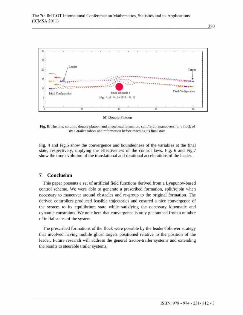
The leader is chosen arbitrarily from the flock. The members of the flock move towards their ghost targets positioned relative to their leader. The corresponding initial and final states and other details for the simulation are listed in Table 1 (assuming that appropriate units have been taken into account). From the initial configuration, the members of the flock quickly move into a desired formation. Upon encountering an obstacle, the members split from their designated formation and maneuver around the obstacles. While avoiding the two obstacles, the members maintain a collision free avoidance with another member of the flock. After avoidance, the members rejoin the flock into the same prescribed formation. Several formations of a team of six 1-trailer robots are considered (Fig 8): • Line – the robots travel line-abreast. • Column – the robots travel one after the other. • Arrowhead – the robots travel in an arrowhead formation. • Double Platoon – the robots travel in double platoon.

Fig. 4. Accelerations: 11σ and 12σ . Fig. 5. Evolution of ( )xL and its time derivative.

Fig. 6. Translational Velocities: 1v , 2v and 6v . Fig. 7. Orientations of the 1st body of the leader and its followers.


ISBN: 978 - 974 - 231- 812 - 3_____________________________________________________________________________________________________

(a) Line

(b) Column

(c) Arrowhead


ISBN: 978 - 974 - 231- 812 - 3_____________________________________________________________________________________________________

(d) Double-Platoon

Fig. 8: The line, column, double platoon and arrowhead formation, split/rejoin maneuvers for a flock of six 1-trailer robots and reformation before reaching its final state.

Fig. 4 and Fig.5 show the convergence and boundedness of the variables at the final state, respectively, implying the effectiveness of the control laws. Fig. 6 and Fig.7 show the time evolution of the translational and rotational accelerations of the leader.

7 Conclusion This paper presents a set of artificial field functions derived from a Lyapunov-based

control scheme. We were able to generate a prescribed formation, split/rejoin when necessary to maneuver around obstacles and re-group to the original formation. The derived controllers produced feasible trajectories and ensured a nice convergence of the system to its equilibrium state while satisfying the necessary kinematic and dynamic constraints. We note here that convergence is only guaranteed from a number of initial states of the system.

The prescribed formations of the flock were possible by the leader-follower strategy that involved having mobile ghost targets positioned relative to the position of the leader. Future research will address the general tractor-trailer systems and extending the results to steerable trailer systems.


ISBN: 978 - 974 - 231- 812 - 3_____________________________________________________________________________________________________

8 References [1] Gazi. V, “Swarm Aggregations Using Artificial Potentials and Sliding Mode Control”,

in Procs. IEEE Conference on Decision and Control, pages 2041-2046, Mauii, Hawaii, (2003).

[2] Crombie. D, “The Examination and Exploration of Algorithms and Complex Behavior to Realistically Control Multiple Mobile Robots”. Master’s thesis, Australian National University, Australia, (1997).

[3] Ogren. P, “Formations and Obstacle Avoidance in Mobile Robot Control”. Master’s thesis , Royal Institute of Technology, Stockholm, Sweden, June (2003).

[4] Edelstein-Keshet. L, “Mathematical Models of Swarming and Social Aggregation”, in Procs. 2001 International Symposium on Nonlinear Theory and its Applications, pages 1-7, Miyagi, Japan, October-November (2001).

[5] Reynolds. C. W, “Flocks, Herds, and Schools: A Distributed Behavioral Model in Computer Graphics”, in Procs. of the 14th annual conference on Computer graphics and interactive techniques, pages 25-34, New York, USA, (1987).

[6] Sharma. B, “New Directions in the Applications of the Lyapunov-based Control Scheme to the Findpath Problem”, PhD Dissertation, University of the South Pacific, Fiji, July 2008.

[7] Sharma. B,Vanualailai. J, and Prasad. A, “Formation Control of a Swarm of Mobile Manipulators”, Rocky Mountain Journal of Mathematics, to appear.

[8] Chang. D. E, Shadden. S. C, Marsden. J. E, and Olfati-Saber. R, “Collision Avoidance for Multiple Agent Systems”, in Procs of the 42nd IEEE Conference on Decision and Control, Maui, Hawaii USA, December (2003).

[9] Kang. W, Xi. N, Tan. J, and Wang. J, (2004) “Formation Control of Multiple Autonomous Robots: Theory and Experimentation”, Intelligent Automation and Soft Computing, 10(2): 1-17.

[10] Olfati-Saber. R, (2006), “Flocking for Multi-agent Dynamic Systems: Algorithms and Theory”, IEEE Transactions on Autonomous Control, 51(3): 401-420.

[11] Olfati-Saber. R and Murray. R. M, “Flocking with Obstacle Avoidance: Cooperation with Limited Information in Mobile Networks”, in Procs. of the 42nd IEEE Conference

on Decision and Control, vol 2, pages 2022-2028, Maui, Hawaii, December (2003). [12] Sharma. B and Vanualailai. J, (2007), “Lyapunov Stability of a Nonholonomic Car-like

robotic System”, Nonlinear Studies, 14(2): 143-160. [13] Sharma. B, Vanualailai. J, Raghuwaiya. K and Prasad. A, (2008), “New Potential Field

Functions for Motion Planning and Posture Control of 1-Trailer Systems”, International Journal of Mathematics and Computing Science, 3(1): 45-71.

[14] Vanualailai. J, Sharma. B, and Ali. A, (2007), “Lyapunov-based Kinematic Path Planning for a 3-Link Planar Robot Arm in a Structured Environment”, Global Journal of Pure and Applied Mathematics, 3(2): 175-190.

[15] Raghuwaiya. K, Singh. S, Sharma. B, and Vanualailai. J, “Autonomous Control of a Flock of 1-Trailer Mobile robots”, in Procs of the 2010 International Conference on Scientific Computing, pages 153-158, Las Vegas, USA, (2010).

[16] Latombe. J-C, Robot Motion Planning, Kluwer Academic Publishers, USA, (1991).


ISBN: 978 - 974 - 231- 812 - 3_____________________________________________________________________________________________________

[17] Sharma.B, Vanualailai. J, and Chand. U, (2009) “Flocking of Multi-agents in Constrained Environments”, European Journal of Pure and Applied Mathematics, 2(3): 401-425.

[18] Brockett. R. W, “Differential Geometry Control Theory”. chapter Asymptotic Stability and Feedback Stabilisation, pages 181-191. Springer-Verlag, (1983).


ISBN: 978 - 974 - 231- 812 - 3_____________________________________________________________________________________________________

formation types of a flock of 1 trailer mobile robots

Documents