formal specification of requirements for analytical
TRANSCRIPT

Graduate Theses, Dissertations, and Problem Reports
2000
Formal specification of requirements for analytical redundancy-Formal specification of requirements for analytical redundancy-
based fault -tolerant flight control systems based fault -tolerant flight control systems
Diego Del Gobbo West Virginia University
Follow this and additional works at: https://researchrepository.wvu.edu/etd
Recommended Citation Recommended Citation Del Gobbo, Diego, "Formal specification of requirements for analytical redundancy-based fault -tolerant flight control systems" (2000). Graduate Theses, Dissertations, and Problem Reports. 2378. https://researchrepository.wvu.edu/etd/2378
This Dissertation is protected by copyright and/or related rights. It has been brought to you by the The Research Repository @ WVU with permission from the rights-holder(s). You are free to use this Dissertation in any way that is permitted by the copyright and related rights legislation that applies to your use. For other uses you must obtain permission from the rights-holder(s) directly, unless additional rights are indicated by a Creative Commons license in the record and/ or on the work itself. This Dissertation has been accepted for inclusion in WVU Graduate Theses, Dissertations, and Problem Reports collection by an authorized administrator of The Research Repository @ WVU. For more information, please contact [email protected].

Formal Specification of Requirements for
Analytical Redundancy based
Fault Tolerant Flight Control Systems
Diego Del Gobbo
Dissertation submitted to theCollege of Engineering and Mineral Resources
at West Virginia Universityin partial fulfillment of the requirements
for the degree of
Doctor of Philosophyin
Aerospace Engineering
Marcello Napolitano, Ph.D., ChairLarry Banta, Ph.D.Robert Bond, Ph.D.
Ali Mili, Ph.D.Gary Morris, Ph.D.
Department of Mechanical and Aerospace Engineering
Morgantown, West Virginia2000
Keywords: Fault Tolerance, Flight Control System, Analytic Redundancy,System Requirements Specification, Relational Algebra
Copyright 2000 Diego Del Gobbo

Abstract
Formal Specification of Requirementsfor Analytical Redundancy based
Fault Tolerant Flight Control Systems
By Diego Del Gobbo
Flight control systems are undergoing a rapid process of automation. The use
of Fly-By-Wire digital flight control systems in commercial aviation (Airbus 320 and
Boeing FBW-B777) is a clear sign of this trend. The increased automation goes in par-
allel with an increased complexity of flight control systems with obvious consequences
on reliability and safety. Flight control systems must meet strict fault-tolerance re-
quirements. The standard solution to achieving fault tolerance capability relies on
multi-string architectures. On the other hand, multi-string architectures further in-
crease the complexity of the system inducing a reduction of overall reliability.
In the past two decades a variety of techniques based on analytical redundancy
have been suggested for fault diagnosis purposes. While research on analytical redun-
dancy has obtained desirable results, a design methodology involving requirements
specification and feasibility analysis of analytical redundancy based fault tolerant
flight control systems is missing.
The main objective of this research work is to describe within a formal frame-
work the implications of adopting analytical redundancy as a basis to achieve fault
tolerance. The research activity involves analysis of the analytical redundancy ap-
proach, analysis of flight control system informal requirements, and re-engineering
(modeling and specification) of the fault tolerance requirements. The USAF mili-
tary specification MIL-F-9490D and supporting documents are adopted as source for
the flight control informal requirements. The De Havilland DHC-2 general aviation
aircraft equipped with standard autopilot control functions is adopted as pilot appli-
cation. Relational algebra is adopted as formal framework for the specification of the
requirements.
The detailed analysis and formalization of the requirements resulted in a better
definition of the fault tolerance problem in the framework of analytical redundancy.
Fault tolerance requirements and related certification procedures turned out to be
considerably more demanding than those typically adopted in the literature. Fur-
thermore, the research work brought up to light important issues in all fields involved
in the specification process, namely flight control system requirements, analytical
redundancy, and requirements engineering.

Acknowledgments
I would like to thank Dr. Marcello Napolitano, my advisor, for his support during this
research. I am thankful to Dr. Ali Mili for having brought some light in the chaos
that characterized the early phases of this work. His guidance was crucial to the
successful completion of this project. I am also thankful to Dr. Francesco Nasuti for
his friendship and for the numerous helpful discussions on the many faces of analytical
redundancy.
I wish to thank all of the Drs., researchers, and students who played a role in this
research work. Among them I would like to cite Dr. Wu Wen, Dr. Jack Callahan, Dr.
Steve Easterbrook, Dr. Bojan Cukic, Dr. Mark Shereshevsky, Dr. Harjinder Sandhu,
and Dr. Vittorio Cortellessa. In the years of meetings and discussions since the start
of the project, they helped me understand the hidden truth behind a multidisciplinary
research work.
I have no words to thank my wife Teresa, without her love and support I would
not be here now. Of course, I am grateful to my parents for their unbounded love,
and to my grandmother for ”being the origin of the family”, as she says. I am also
grateful to my brothers for not hanging me upside down this time, and to my sister
for her unforgettable shout of joy.
Finally, I wish to thank all of those who kept asking: ”So ... have you done?” ...
I have!
iii

Contents
1 Introduction 1
2 Background information 52.1 Issues on the analytical redundancy approach in fault tolerant flight
control systems . . . . . . . . . . . . . . . . . . . . . . . . . . . . . . 62.1.1 Analytical redundancy . . . . . . . . . . . . . . . . . . . . . . 62.1.2 Analytical redundancy in flight control systems . . . . . . . . 9
2.2 Formal specification of system requirements . . . . . . . . . . . . . . 122.2.1 Requirements engineering . . . . . . . . . . . . . . . . . . . . 122.2.2 Advantages of adopting a formal specification language . . . . 16
3 Research framework 183.1 FTC: the system to be specified . . . . . . . . . . . . . . . . . . . . . 18
3.1.1 FTC environment . . . . . . . . . . . . . . . . . . . . . . . . . 193.1.2 Main functions of the FTC system . . . . . . . . . . . . . . . 213.1.3 FTC interface with its environment . . . . . . . . . . . . . . . 26
3.2 DHC-2 aircraft . . . . . . . . . . . . . . . . . . . . . . . . . . . . . . 293.3 Military specification for AFCS . . . . . . . . . . . . . . . . . . . . . 31
4 Formal specification of the FTC environment 354.1 Relational specification of elementary requirements . . . . . . . . . . 364.2 Composition of elementary requirements . . . . . . . . . . . . . . . . 454.3 Formal specification of the FTC environment . . . . . . . . . . . . . . 51
4.3.1 Performance requirement composition . . . . . . . . . . . . . 544.3.2 DHC-2 detail-specification . . . . . . . . . . . . . . . . . . . . 564.3.3 Correctness of AFCS design . . . . . . . . . . . . . . . . . . . 60
5 Formal requirements specification of the FTC 625.1 FTC requirements . . . . . . . . . . . . . . . . . . . . . . . . . . . . 62
5.1.1 FTC functional requirements . . . . . . . . . . . . . . . . . . 625.1.2 FTC non-functional requirements . . . . . . . . . . . . . . . . 665.1.3 FTC-AR requirements . . . . . . . . . . . . . . . . . . . . . . 67
5.2 Formal specification of FTC-AR . . . . . . . . . . . . . . . . . . . . . 715.2.1 Components partitioning . . . . . . . . . . . . . . . . . . . . . 715.2.2 Formal specification of fault hypotheses . . . . . . . . . . . . . 74
iv

5.2.3 Relational specification of the FTC-AR requirements . . . . . 755.3 Feasibility analysis . . . . . . . . . . . . . . . . . . . . . . . . . . . . 77
5.3.1 Traditional interpretation of detectability and identifiability . 785.3.2 Formal definition of detectability and identifiability . . . . . . 80
6 Conclusions 82
A Predicate Logic and Relational Algebra 92A.1 Logic . . . . . . . . . . . . . . . . . . . . . . . . . . . . . . . . . . . . 92
A.1.1 Propositional logic . . . . . . . . . . . . . . . . . . . . . . . . 92A.1.2 Predicate logic . . . . . . . . . . . . . . . . . . . . . . . . . . 93
A.2 Relational algebra and requirements specification . . . . . . . . . . . 95A.2.1 Basics of relational algebra . . . . . . . . . . . . . . . . . . . 95A.2.2 Relational specifications . . . . . . . . . . . . . . . . . . . . . 97
B Elementary specifications of the AR-FTC environment 102B.1 Elementary requirements of AFCS performance specification . . . . . 103B.2 Elementary requirements of DHC-2
detail-specification . . . . . . . . . . . . . . . . . . . . . . . . . . . . 113B.2.1 DHC-2 airplane dynamics . . . . . . . . . . . . . . . . . . . . 113B.2.2 DHC-2 Flight Control System Hardware . . . . . . . . . . . . 119B.2.3 DHC-2 Flight Control System Software . . . . . . . . . . . . 126
B.3 Fault modes . . . . . . . . . . . . . . . . . . . . . . . . . . . . . . . . 130B.3.1 Control-surface fault modes . . . . . . . . . . . . . . . . . . . 130B.3.2 Engine fault modes . . . . . . . . . . . . . . . . . . . . . . . . 131B.3.3 Actuator fault modes . . . . . . . . . . . . . . . . . . . . . . . 131B.3.4 Rate gyro fault modes . . . . . . . . . . . . . . . . . . . . . . 132B.3.5 Accelerometer fault modes . . . . . . . . . . . . . . . . . . . . 133B.3.6 Air data sensor fault modes . . . . . . . . . . . . . . . . . . . 133B.3.7 Angle of attack sensor fault modes . . . . . . . . . . . . . . . 134B.3.8 Attitude and heading sensor fault modes . . . . . . . . . . . . 134
B.4 DHC-2 requirement space restriction sets . . . . . . . . . . . . . . . 136B.5 Elementary requirements of interface blocks to AR-FTC system . . . 138
C Support tables of the specification 141
v
List of Tables
3.1 DHC-2 autopilot functions and related controls . . . . . . . . . . . . 30
4.1 Constants used within the specification of the HH function. . . . . . . 414.2 Domain and image variables used within the specification of the HH
function. . . . . . . . . . . . . . . . . . . . . . . . . . . . . . . . . . . 414.3 Quantified variables used within the specification of the HH function. 414.4 Predicates and functions used within the specification of the HH function. 41
A.1 Syntax of propositional logic . . . . . . . . . . . . . . . . . . . . . . . 93A.2 Semantics of propositional logic . . . . . . . . . . . . . . . . . . . . . 94A.3 Syntax of predicate logic . . . . . . . . . . . . . . . . . . . . . . . . . 94
B.1 Minimum acceptable control accuracy for ALH function . . . . . . . . 111
C.1 Elementary requirements . . . . . . . . . . . . . . . . . . . . . . . . 143C.2 Composed requirements . . . . . . . . . . . . . . . . . . . . . . . . . 149C.3 Fault modes . . . . . . . . . . . . . . . . . . . . . . . . . . . . . . . 150C.4 Restriction sets . . . . . . . . . . . . . . . . . . . . . . . . . . . . . . 151C.5 Spaces used within the requirements specification . . . . . . . . . . . 152C.6 Domain and image variables . . . . . . . . . . . . . . . . . . . . . . . 154C.7 Constants . . . . . . . . . . . . . . . . . . . . . . . . . . . . . . . . . 161C.8 Quantified variables . . . . . . . . . . . . . . . . . . . . . . . . . . . 172C.9 Auxiliary terms . . . . . . . . . . . . . . . . . . . . . . . . . . . . . . 176C.10 Data-types . . . . . . . . . . . . . . . . . . . . . . . . . . . . . . . . 182
vi
List of Figures
3.1 Environment of the FTC system. . . . . . . . . . . . . . . . . . . . . 193.2 FTC within its environment. . . . . . . . . . . . . . . . . . . . . . . . 273.3 Block diagram of DHC-2 aircraft and its FCS. . . . . . . . . . . . . . 32
4.1 Sample requirements specification structure. . . . . . . . . . . . . . . 464.2 Structure of the AFCS performance requirements specification. . . . . 554.3 Structure of the DHC-2 detail-specification. . . . . . . . . . . . . . . 58
5.1 DHC-2 and FTFCS requirements specification structure. . . . . . . . 68
vii
List of Symbols and Abbreviations
ACT ActuatorADC Analog to Digital ConverterAFCS Automatic Flight Control SystemALH Altitude HoldAR Analytical RedundancyAR-FTFCS Analytical Redundancy based Fault Tolerant Flight Control SystemCP Control PanelCin Computer inputCout Computer outputDAC Digital to Analog ConverterDHC-2 De Havilland DHC-2 aircraftDP Display PanelFBW Fly-By-WireFCC Flight Control ComputerFCL Flight Control LawFCS Flight Control SystemFCSw Flight Control SoftwareFDC Flight Dynamics and ControlFTC Fault Tolerance CapabilityFTC-ADC Fault Tolerance Capability – Analog to Digital ConverterFTC-AR Fault Tolerance Capability – Analytical Redundancy moduleFTC-CP Fault Tolerance Capability – Control Panel moduleFTC-DAC Fault Tolerance Capability – Digital to Analog ConverterFTC-DP Fault Tolerance Capability – Display Panel moduleFTC-IN Fault Tolerance Capability – software Input interfaceFTC-OUT Fault Tolerance Capability – software Output interfaceFTC-SW Fault Tolerance Capability – Safety switchFTFCS Fault Tolerant Flight Control SystemHH Heading HoldHS Heading SelectMFCS Manual Flight Control SystemPAH Pitch Attitude HoldRAH Roll Attitude HoldUAV Unmanned Aerial Vehicle
viii

Infallible / fail-operational software component
Infallible / fail-operational hardware component
Subsystem made of more than one component
Fallible hardware component
Directional data stream
Infallible / fail-operational software component of FTC system
Infallible / fail-operational hardware component of FTC system
Physics law
��
Note: Symbols used in the document are collected in the tables of Appendix C
ix

Chapter 1
Introduction
The use of Fly-By-Wire (FBW) digital flight control systems is playing a more and
more prominent role in commercial aviation. Airbus and Boeing FBW-airliners pro-
vide a clear sign of this trend. In FBW technology electronic devices coupled to
a digital computer replace conventional mechanical controls. The net result is a
more efficient, easier to control aircraft. However, this increased automation goes in
parallel with an increased complexity of flight control systems with obvious conse-
quences on reliability and safety. A FBW flight control system is made up of several
subsystems including mechanical, electronic, and software components. Each of these
subsystems may fail during flight, with disastrous consequences. For this reason flight
control systems must meet strict fault-tolerance requirements. The standard solution
to achieving fault tolerance capability is the adoption of a multi-string architecture.
This architecture is based on redundant units working in parallel and a voting scheme
that disengages a unit when faulty. Triple and quadruple string architectures are cur-
rent practice in flight control systems of both military and commercial aviation [62],
[21]. On the other hand, multi-string architectures further increase the complexity
of the system, induce a reduction of overall reliability, bind to closer maintenance
1
schedule, and require larger budgets. These factors have induced in recent years an
increased interest toward alternative approaches to achieving fault tolerance in flight
control systems.
Similar interest comes from fields related to satellite and Unmanned Aerial Ve-
hicle (UAV) applications. Under the ongoing process of globalization the telecom-
munication industry is growing without rest and commercial satellites are playing
an important role in this growth. Weight and size largely affect launching costs of
satellites. Weight and size also affect UAV applications. Starting in the late ’80s a
variety of UAVs have been built for either military or scientific purposes. They vary
significantly in size, mission profile, and payload weight carrying capability. With
some of them having a payload weight below 20 lbs and dimensions below 15 feet it is
clear how weight and room requirements are a major issue. Despite costs, complexity,
and weight drawbacks physical redundancy is adopted to achieve fault tolerance.
Redundancy is a must in achieving fault tolerance; the question is whether re-
dundancy other than physical can be adopted. In the past two decades a variety of
techniques based on analytical redundancy have been suggested for fault diagnosis
purposes. Analytical redundancy identifies with the functional redundancy of the sys-
tem. No extra hardware is required; fault tolerance is achieved by means of software
routines that process sensor outputs and actuator inputs to check for consistency
with respect to the analytical model of the system. If an inconsistency is detected,
the faulty component is isolated and the control law is reconfigured accordingly. The
first analytical redundancy scheme implemented within a flight control systems dates
2
back to the 70’s, when the same aircraft used to conduct research on fly-by-wire tech-
nology was also used as testbed for an analytical redundancy management algorithm
[56]. The algorithm showed desirable performance during flight test; however, poor
robustness to modeling errors and the degree of modeling necessary retrained further
development. Since then, a number of results have been obtained in the area of robust
fault diagnosis [47]. While research on analytical redundancy has been obtaining de-
sirable results, a design methodology involving requirements specification, feasibility
analysis, and certification of analytical redundancy based fault tolerant flight control
systems is still missing. Exploring strengths, weaknesses, related degree of reduction
of physical redundancy, and overall reliability is a fundamental step in the engineering
of such systems.
The main objective of this research is to describe within a formal framework the
relevant aspects of Analytical Redundancy based Fault Tolerant Flight Control Sys-
tems (AR-FTFCS) to allow the analysis of the implications of adopting the analytical
redundancy approach to achieve fault tolerance. The outcome of the research identi-
fies with the requirements specification for an AR-FTFCS.
The De Havilland DHC-2 general aviation airplane equipped with standard au-
topilot control functions is adopted as pilot application. The steps of the research
work are those typical of requirements engineering: analysis of the problem and elic-
itation of the requirements, requirements modeling, and requirements specification.
The USAF military specification MIL-F-9490D [2] and supporting documents are
adopted as source for the autopilot performance and fault tolerance requirements.
3
[37] and [53] are adopted to produce the detail-specification of the DHC-2. The im-
plications of adopting the analytical redundancy approach are analyzed in detail to
modify the fault tolerance requirements accordingly. Relational algebra is adopted as
formal framework for the specification of the requirements.
Given the multidisciplinary nature of the research work some background infor-
mation is provided. Analytical redundancy is introduced in Chapter 2; the focus is
on the implications of adopting the analytical redundancy approach in flight control
systems. The flaws of the fault-diagnosis design approach and of the evaluation pro-
cedures for AR-FTFCS are highlighted. The second part of the chapter introduces
the main concepts of requirements engineering and briefly discusses the advantages of
adopting a formal specification language. Appendix A provides a description of pred-
icate logic and relational algebra. The FCS fault tolerance requirements as specified
in [2] are illustrated in Chapter 3. In the same chapter the target of the requirements
specification is defined and an introductory analysis of the implication of adopting
analytical redundancy is performed. Chapter 4 provides a detailed description of the
re-engineering and formalization process of the requirements. The composition of the
AFCS performance specification and of the DHC-2 detail-specification is illustrated.
In Chapter 5 the analysis of the fault tolerance requirements is carried out one step
further and the formal specification of the system providing fault tolerance is devel-
oped. Appendix B contains the bulk of the specification, while appendix C contains
the related supporting tables.
4

Chapter 2
Background information
This chapter provides some introductory information about two concepts that play
a central role in this research work: analytical redundancy and requirements engi-
neering. The first section provides a definition of analytical redundancy and briefly
illustrates the most relevant techniques adopting analytical redundancy as a basis
for fault tolerance. The focus is mainly on closed loop systems. A discussion about
the implications of adopting analytical redundancy to achieve fault tolerance in flight
control systems follows. The second section provides an introduction to the require-
ments engineering discipline. It illustrates the role of requirements specification in
the system life-cycle, the main phases of requirements engineering, and the agents
involved in the requirements specification process. The chapter closes with a brief
discussion about the advantages of adopting a formal specification language.
5
2.1 Issues on the analytical redundancy approach
in fault tolerant flight control systems
2.1.1 Analytical redundancy
Fault tolerance requires some form of redundancy within the system; redundancy pro-
vides alternative means to perform a specific task, thus making the system capable of
continuing operation despite of localized malfunctions, i.e. of tolerating faults. Two
different redundancy approaches are adopted in closed loop system: physical redun-
dancy and analytical redundancy. Physical redundancy is based on a multichannel
architecture consisting of three or more intercommunicating systems that are able to
work independently. A voting mechanism checks for consistency among the redundant
components of each channel. Analytical redundancy identifies with the functional re-
dundancy in the system dynamics. It does not require additional hardware; fault
tolerance is achieved by means of software routines that process sensor outputs and
actuator inputs to check for consistency with respect to the analytical model of the
system. If an inconsistency is detected, the faulty component is isolated and the
control law is reconfigured accordingly. Preserved observability allows estimating the
measurement of an isolated (allegedly faulty) sensor, while preserved controllability
allows controlling the system with an isolated (allegedly faulty) actuator. Numerous
survey papers and books [52], [11], and [51] discuss theoretical and practical aspects
of adopting the analytical redundancy approach to achieve fault tolerance.
The conceptual structure of an analytical redundancy based fault detection and
identification systems consists of two stages: the residual generation stage and the
6
decision making stage [14]. The residuals provide a measure of the inconsistency
between the actual behaviour of the system and the system analytical model. Residual
values close to zero imply a fault free system; on the other hand, residual values
different from zero reveal a fault within the system, and the particular combination
of residual values provides means for isolating the faulty component. Processing of the
residuals to perform fault detection and isolation is the main task of the decision stage.
Decision algorithms range from simple threshold testing on the instantaneous values
or on the moving average of the residuals, to more sophisticated statistical testing
based on the Generalized Likelihood Ratio test [60], or on the Sequential Probability
Ratio test [8]. To achieve fault tolerance an additional recovery stage needs to be
added. This stage consists of an adaptive or multi-model control law that processes
information provided by the decision making stage to produce a suitable control
law. All of the three stages play an equally important role toward the successful
fault tolerant control system; however, most of the research focuses on the residual
generation problem.
Since the early 70’s a variety of residual generation techniques have been sug-
gested in the technical literature. The first techniques adopted a geometric approach
that resulted in what is known as the Beard-Jones Fault Detection Filter [60]. The
detection filters are designed to generate a residual vector with a different direction
for each faulty component, thus allowing both detection and isolation. Design issues
for such filters are addressed in [46] and [45]. Another approach based on the de-
terministic description of the system is the dedicated observer approach [16]. This
7

scheme can be adopted for achieving fault tolerance with respect to sensor failures.
It is based on a bank of observers each processing a subset of the sensor readings and
producing an estimate of the system state vector. Detection and isolation are per-
formed by comparing the state vector estimates produced by the different observers.
In its first applications this scheme was implemented by using Luenberger observers;
then the scheme was extended to non-linear observers [22], Kalman filters [61], and
neural-network based estimators [41]. The parity relation approach is based on the
design of invariant relations among system inputs and outputs on the basis of the
matrices of the system state space model ([15], [12], and [25]). All of the mentioned
approaches focus on the system inputs, outputs, or state variables to produce the
residual vector. A different approach based on parameter estimation focuses on es-
timating unmeasureable system parameters that are directly related to the source of
the fault [33]. The differences among the above techniques are mostly of conceptual
nature; studies have shown the practical equivalence of parity relation and observer
based approaches [48], and of parity relation and parameter estimation approaches
[27].
The weakness of early analytical redundancy based residual generators is in the
sensitivity to process disturbances, and in the low performance for non-linear sys-
tem applications. The unknown input observer approach [23] is the first attempt to
produce a robust fault detection scheme; it focuses on generating a residual vector
that is de-coupled from disturbance inputs. Later on robustness was introduced in
the design of parity relation based schemes leading to the orthogonal parity relation
8

concept [28]. Robustness needs lead to a shift of the design into the frequency do-
main to adopt optimal and robust design techniques like H∞ [18] and µ synthesis [7].
To address the non-linearity issue researchers extended linear design techniques or
adopted approaches based on fuzzy logic [50] and neural networks [57] and [39].
2.1.2 Analytical redundancy in flight control systems
Analytical redundancy approach to fault detection has been adopted in a variety of
different fields ranging from automotive engines [26] to electromechanical actuators,
induction motor drives, electrical pumps, pipelines [34], chemical processes, heat ex-
changers [30], gas turbine engines, aircraft jet engine sensors [49], etc. Analytical
redundancy has also been used in flight control systems; the very same aircraft used
to conduct research on fly-by-wire technology was also used as testbed for an analyti-
cal redundancy based fault detection algorithm ([17] and [56]). Since then, a number
of results have been published on the suitability of analytical redundancy approach for
reconfiguration of flight control systems ([59] and [10]), and for diagnosis of aircraft
actuator and sensor failures ([54] and [40]). Nevertheless, doubts remain on the pos-
sibility that analytical redundancy based solutions can meet the strict fault tolerance
requirements of flight control systems [44]. Section 3.1.2 illustrates such requirements
as formulated in the active military specification for piloted flight control systems [2].
There is a considerable difference between the fault tolerance requirements of flight
control systems and those of of the other applications mentioned above. Fault toler-
ance in the terms typical to fault detection and identification literature [11] aims at
enhancing system reliability and availability by monitoring unreliable components of
9

the system under the assumption that the other components are working properly. A
similar perspective has been erroneously adopted in designing analytical redundancy
based fault tolerant in flight control systems. Reliability enhancement and dedicated
monitoring of unreliable components are not the key issues in fault tolerant flight
control systems. In such systems fault tolerance requires the capability of continued
operation after failure of any of the system components (section 6.6 of [3]). Fault-free
assumption on any of the system components is not allowed unless failure of these
components is proven to be extremely remote [2]. Civil and military aircraft equipped
with fly-by-wire flight control systems adopt physical redundancy to achieve fault tol-
erance. Triple and quadruple redundancy is adopted in the Airbus 320 [21] and in the
Boeing FBW-B777 [62] to meet fault tolerance requirements. Increased complexity
of physical redundant systems brings a degradation of overall system reliability; but
the focus is on safety, not on reliability.
Another problem with analytical redundancy is related to the process of per-
formance evaluation of fault tolerant systems adopting such approach. Since these
systems exploit the functional redundancy of the plant, when applied in the field of
flight control systems they need to be validated over the entire aircraft operational
envelope. Instead, most of these solutions are evaluated using a simplified model
of the aircraft dynamics, within a limited region of the flight envelope, and with a
limited set of maneuvers and fault-modes. Furthermore, evaluation criteria are quite
heuristic. A tentative list of criteria for assessing the performance of fault detection
and identification systems can be found in [52], and is summarized below:
10

• promptness of detection
• sensitivity to incipient failure
• false alarm rate
• missed fault detection
• incorrect fault identification
A typical testing procedure for fault detection and identification systems involves
injection of a set of failures within a simulation environment and computation of
the above indexes. While obtained values can be effectively used to compare the
performance of two different solutions, they have no absolute interpretation. The
testing environment has a considerable impact on the evaluation of these indexes.
Missed detection and false alarm rate do not provide any valuable information if
they are not determined within the operational envelope of the system. These figures
are highly dependent on the disturbances acting on the system, on the type of fault
injected, and – for non linear systems – on the state of the system. Furthermore, the
fault could be not detectable at all, thus leading to a missed rate of 100%. But this
value is not an index of poor performance of the fault detection system; rather, it
indicates a lack of functional redundancy within the system.
In order to provide an objective basis for the evaluation of analytical redundancy
based fault tolerant flight control systems it is mandatory to develop the requirements
specification for such systems. Validation of a system can be performed only against
its specification.
11

2.2 Formal specification of system requirements
2.2.1 Requirements engineering
A successful system is a system that fully addresses the needs for which it was built.
Requirements engineering is the process that discovers those needs, and documents
them in a form that is suitable for analysis, communication, and subsequent imple-
mentation [42]. For a comprehensive evaluation of the role of the requirements in
the development of a system it is important to have a clear understanding of the
system life-cycle. The system life-cycle consists of three cycles: the concept cycle, the
development cycle, and the operation cycle [35]. The first cycle involves outlining the
main functions of the system and investigating its feasibility. The development cycle
involves requirements specification, design, implementation, and testing (or certifi-
cation). The operation cycle spans the time from system certification to retirement
from service. The requirements specification phase takes place between the concept
phase and the design phase. It transforms the informal, incomplete, and ambiguous
needs, as expressed in the concept phase, into a set of requirements that serve as
the supporting document for the subsequent phases of design, testing, and operation.
The design phase transforms required functions into algorithms and physical pro-
cesses that are transformed within the implementation phase into software code and
hardware components. The testing phase aims at determining whether the system
meets all requirements; successful certification implies that the system will meet its
operational phase commitments.
Though requirements specification and design play different roles within the de-
12
velopment cycle they are not separated in time. The system is decomposed into a
hierarchy of elements on a functional basis according to the principle of architectural
design [19] . Requirements engineering concerns with all elements at all levels. Steps
of requirements analysis and design alternate throughout the hierarchical structure
of the system to produce a sequence of requirements specifications corresponding
to different levels in the decomposition. The prominent role of the requirements
specification throughout the development cycle and the consequences of inadequate
specification has been widely documented in the literature: ”... No other part of the
work so cripples the resulting system if done wrong. No other part is as difficult to
rectify later.” [20] ”requirements inadequacies play a major and expensive role in a
project failure” [19].
The main activities of requirements engineering are [19]:
• elicitation
• analysis and modeling
• specification
• validation
• management
Elicitation consists in identifying what problems the system needs to address and
in outlining the boundaries between the system and its environment. The modeling
activity consists in the development of an abstract description of the system and its
13
environment. The system environment is the part of the world with which the system
will interact and in which the effect of the system are evaluated; its description plays
a fundamental role in the requirements specification. System requirements are condi-
tions over phenomena of the environment [36]; shared phenomena are the phenomena
that belong to both entities while private phenomena belong exclusively to the envi-
ronment. Requirements are conditions over both shared and private quantities. The
system can assure satisfaction of requirements involving private quantities thanks to
environment properties that relate private phenomena to shared phenomena. These
properties are called the indicative properties of the environment and they are true
irrespective of the presence of the system, as opposed to the optative properties that
need to be guaranteed by the system and that are captured by the requirements. Only
by describing the environment it is possible to describe the purpose of the system and
provide the information required to its design.
The specification activity involves the formulation of the requirements by means
of a specification language. There is a variety of formal and informal languages
adopted in requirements engineering; the advantages of adopting a formal specifica-
tion language are discussed in the next section. The validation activity consists in
establishing whether the requirements specification is complete, correct, unambigu-
ous, consistent, testable, and feasible [9]. Completeness and correctness provide that
the requirements specification captures the purpose of the system within its envi-
ronment. Evaluation of completeness is problematic because it involves a subjective
judgment of how well a system that meets the requirement addresses the real-world
14

need. Absence of ambiguity, consistency, and testability can be obtained by adopting
a formal specification language. Requirements feasibility needs to be evaluated by
the domain experts. To save efforts and resources it is important to determine ahead
of time whether a system can be built that meets the requirements. The last activity
of requirements engineering is requirements management. In practice it is impossible
to develop a specification that remains stable throughout the life-cycle of the system.
Efficient management of requirements plays a crucial role in managing requirements
evolution in time and in providing traceability. The IEEE Guide for Developing Sys-
tem Requirements specifications [6] provides guidelines to proper structuring of the
specification document to facilitate modifications. However, given the considerable
dimension that specification documents usually reach, management of specification
without well engineered tools is not feasible.
A peculiar feature of requirements engineering is its multidisciplinary nature.
Three different agents are typically involved in the requirements engineering process:
the customers, the domain experts, and the requirements engineers. The customers
are those interested in addressing the real-world problem; they provide a raw defini-
tion of the requirements that typically is the result of the concept phase of the system
life-cycle. The domain experts are those involved in the activity of design, implemen-
tation, integration, and testing. Their contribution in the requirements specification
process is essential since they provide the technical know-how to decompose the sys-
tem into a suitable hierarchical structure, to analyze and model the requirements, and
to assess feasibility of the requirements. The requirements engineers work in strict
15

collaboration with the customers to elicit the requirements and collaborate with the
domain experts to perform analysis and modeling of the requirements. Specification,
validation, and management are in prevalence tasks of the requirements engineers
though some validation tasks involve all three agents. The requirements specification
document is the official means of communication between the three agents. It collects
all the information required to design the system along with the acceptance criteria
that will be used to verify whether the system addresses the real-world need.
2.2.2 Advantages of adopting a formal specification language
The requirements specification involves a considerable amount of engineering analysis
and judgement, it is the result of a long sequence of refinements, it is produced with
the collaboration of personnel in different area of expertise, and typically results in
a voluminous document with a complex set of dependencies. These factors make it
difficult to produce a consistent and unambiguous requirements specification. Despite
the considerable expressive power of plain-English, its use as specification language
introduces an additional source of ambiguity and inconsistency. Considerable leverage
can be obtained by adopting a formal specification language. A formal language is
a language with a mathematically defined syntax and semantics. The mathematical
definition of the language potentially eliminates the ambiguity problem, allows for
checking the consistency of the specification, and leads to a specification amenable to
automated analysis. Furthermore, the rigid structure of the formal specification serves
as a guide in formulating the requirements resulting in a homogeneous document
throughout the refinement iterations.
16

Improvements obtained by adopting a formal language do not come without a
cost. Formal specification of a requirement must be explicit in all its parts and this
usually results in an even more bulky document. Furthermore, interpretation of a
formal specification is not straightforward resulting in a diminished effectiveness of
the communication capability of the document.
A suitable specification language should be expressive, that is it should be possi-
ble to formalize plain-English requirements without introducing artifacts. It should
not introduce modeling constraints that could bias the specification structure. It
should be monotonic so that the specification can be obtained by composition of sub-
specifications; this feature guarantees ease of update during the development cycle.
It should be supported by well engineered tools for automatic checking of consistency
and for management.
The specification language adopted in this research work is based on predicate
logic and relational algebra and is defined in Appendix A
17

Chapter 3
Research framework
In Chapter 1 it was stated that the target of this research work is the development
of a formal requirements specification for a FTFCS where fault tolerance is achieved
by exploiting analytical redundancy; in these terms, the target is quite vague and
imprecise. In this chapter the target is refined by introducing the environment of
the system the author has developed the specification for, and most of all, by elab-
orating on the function of the system within its environment. In this chapter the
author also introduces the aircraft that will serve as pilot application in developing
the specification, and the military specification that will serve as main source for
AFCS performance and fault tolerance requirements.
3.1 FTC: the system to be specified
In order to specify the requirements for any system it is critical to describe the system
environment, mark the boundaries of the system within the environment, and describe
the main functions of the system within the environment. The system under analysis
is the aggregate of hardware and software components that is added to the AFCS to
provide Fault Tolerance Capability (FTC). From now on the acronym FTC is used
18

controlpanel
displaypanel
Cout Cin
FCSw
DAC ADC
Airframe
������secondary
sensors������actuators
����
controlsurfaces
FCL INOUT
����engines
������primarysensors
FCCAFCS
Aircraft
displaypanel
controlpanel
Figure 3.1: Environment of the FTC system.
to identify such system.
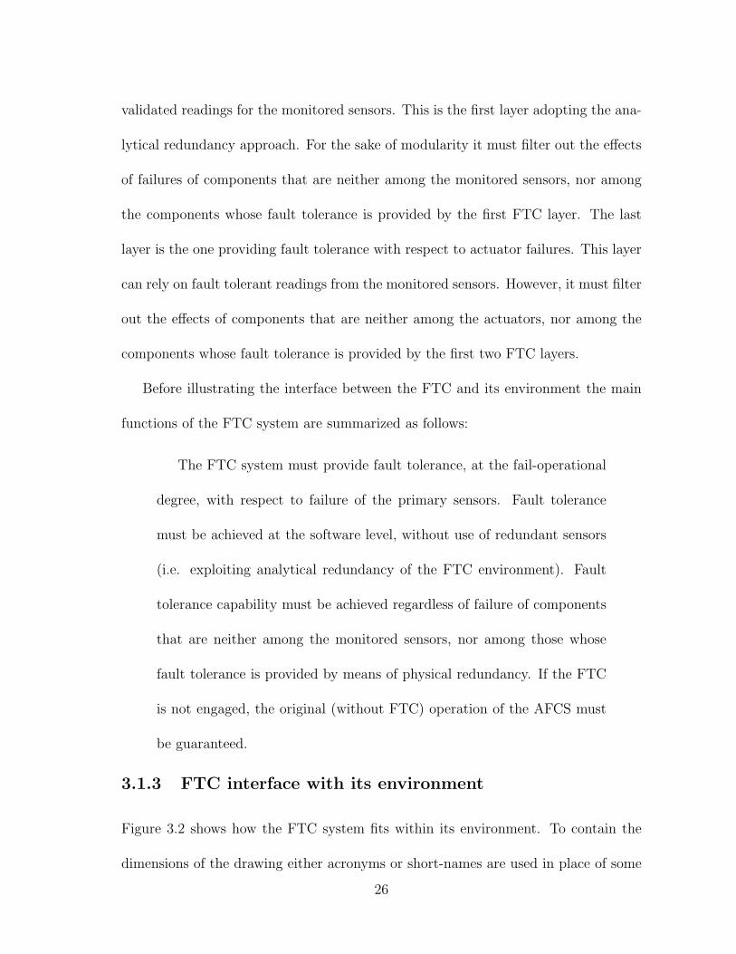
3.1.1 FTC environment
The environment of the FTC is the AFCS along with the whole aircraft dynamics.
Figure 3.1 shows a functional block diagram of an aircraft equipped with an AFCS.
The arrows in the diagram represent data streams like forces and moments, electrical
signals, software data, etc; the blocks represent processing units. Square-corner blocks
represent hardware units, while round-corner blocks represent software units. Blocks
19

are grouped by means of dash-lines to form subsystems or systems.
The aircraft system represents the aggregate of airframe, control surfaces, and
engines. The control surfaces are typically included in the airframe; here they are
separated since different fault hypotheses are introduced for the two units. The air-
frame block also includes the contribution of gravitational field and air turbulence
to the aircraft dynamics. The group of blocks marked AFCS represents the auto-
matic flight control system. It is composed of the flight control computer (FCC),
the subsystem processing computer-output (Cout), and the subsystem generating
computer-input (Cin). The FCC is composed of the Flight Control Software (FCSw)
and of the DAC and ADC blocks. The last two blocks represent the transformation
from electrical signals to software data and viceversa. The FCSw is composed of three
units: IN, OUT and FCL (Flight Control Law). IN and OUT serve as pre-processing
and post-processing units to the flight control law, while FCL is the block that pro-
cesses software representation of pilot inputs and sensor outputs to produce a software
representation of the input to the actuators, the engines, and the display panel. The
Cin and Cout subsystems contain blocks whose names are self-explanatory. The set of
sensors is separated in primary and secondary sensors. The primary sensors are those
that produce measurements used within the FCL. Measurements from secondary sen-
sors, instead, are used for other purposes, eventually from another control law not
shown in the diagram.
The block diagram of Figure 3.1 does not represent the physical units of the AFCS
and the related interconnections. Rather, it represents the functions needed within
20

the AFCS. For example, the FCC block may represent three physical computers whose
collective behaviour and interface is that of the FCC block.
3.1.2 Main functions of the FTC system
The failure of any component within the FCS can compromise the safety of the
aircraft. For this reason FCS’s must provide some degree of fault tolerance with
respect to failure of their own components. The military specification for FCS’s [2]
defines three different degrees of fault tolerance that correspond to different degrees of
criticality of the FCS function. In turn, the criticality of a FCS function is defined in
terms of the operational state of the aircraft in the post-failure scenario. The relevant
operational state – as far as fault tolerance is concerned – is state III, defined as
follows:
Operational State III is the state of degraded flight control system per-
formance, safety or reliability which permits safe termination of precision
tracking or maneuvering tasks, and safe cruise, descent and landing at
the destination of original intent or alternate but where pilot workload is
excessive or mission effectiveness is inadequate.
Hence, a FCS function is declared:
Essential if loss of the function results in an unsafe condition or inability to maintain
FCS Operational State III
Flight phase essential if loss of the function results in an unsafe condition or in-
ability to maintain FCS Operational State III only during specific flight phases
Non-critical if loss of the function does not affect flight safety or result in control
capability below that required for FCS Operational State III
21
The degrees of fault tolerance for FCS functions are defined as follows:
Fail operational The capability of the FCS for continued operation without degra-
dation following a single failure, and to fail passive in the event of a related
subsequent failure.
Fail passive The capability of the FCS to automatically disconnect and to revert to
a passive state following a failure.
Fail safe The capability of the FCS in a single channel mode of operation to revert
to a safe state following an automatic disconnect in the event of a failure or
pilot initiated disconnect.
Each FCS function is required to provide a certain degree of fault tolerance ac-
cording to its criticality. More specifically, essential FCS functions are required to be
fail operational, flight-phase-essential FCS functions are required to be fail passive,
and non-critical FCS functions are required to be fail safe. In practice these fault
tolerance levels are exceeded for flight-phase-essential and essential controls due to
reliability or flight safety requirements. Here the focus is on fault tolerance only and
neither reliability nor safety requirements are considered .
The FCS functions under anlysis are typical autopilot functions, such as Pitch
Attitude Hold, Roll Attitude Hold, etc. Autopilot FCS’s are non-critical functions;
as such, they are required to be fail safe. Typically, fault tolerance requirements
for autopilot functions are met by monitoring values of sensor readings and of con-
trol inputs to actuators; if these values are over predetermined ranges the autopilot
automatically disengages returning control to the pilot. In this research work autopi-
lot fault tolerance requirements are extended to fail operational capability, with the
22

constraint of adopting the analytical redundancy approach.
Analytical redundancy based fault tolerance is achieved at the software level; soft-
ware routines process control law inputs and outputs to check their consistency against
an analytical model of the controlled system (in this case the aircraft). Analytical
redundancy, however, cannot be used to provide fault tolerance with respect to failure
of all the FCS components. Any component of the FCS, either hardware or software,
can fail. Analytical redundancy cannot help with software failures; nor it can help if
in a single-channel FCS the FCC fails, since the FCC hosts the software that provides
fault tolerance. Failure of either the control or the display panel cannot be accommo-
dated at the software level; hence, analytical redundancy is – under these conditions
– useless. The remaining components of the FCS are the actuators and the sensors.
Analytical redundancy based solutions presented in the literature typically separate
the problems of actuator and sensor failure. The rationale behind this choice is sim-
ple: fault tolerance with respect to sensor failures is mostly an observation problem,
while fault tolerance with respect to actuator failures is mostly a control problem;
different expertise and techniques are required for designing the two different FTC
systems. The author adopts this modular approach and chooses to focus on sensor
failures only. Hence, the FTC system is required to provide fault tolerance with re-
spect to failure of any of the primary sensors. Fault tolerance with respect to failure
of the secondary sensors is not required since secondary sensor outputs are not used
by the FCL.
23

Focusing on sensor failures does not imply that all remaining components of the
FTC environment are not subject to failure. Whether components are subject to
failure or not cannot be arbitrarily established; this is a constraint that is dictated
by the nature of the component. Under the realistic assumption that each FCS
component is subject to failure the question is which redundancy approach should be
adopted to provide fault tolerance. For some of the FCS components fault tolerance
cannot be achieved at the software level; these components are the FCSw, the FCC,
the CP, and the DP. The author assumes that fault tolerance with respect to failure of
these components is achieved by means of physical redundancy, and that performance
requirements are still satisfied following a single failure. On the other hand, the author
assumes that fault tolerance with respect to actuator and sensor failures is achieved
at the software level.
Since analytical redundancy is provided by the functional redundancy within the
aircraft dynamics the impact of failure of the aircraft subsystem components must be
taken into account as well. Control surfaces and engines are assumed to be fallible,
while different hypotheses are made for the airframe. In military aviation partial
separation of wing or tail surfaces is possible in a combat scenario; while in commercial
aviation this is quite an extraordinary event. For this reason the airframe is assumed
infallible. Fallible components whose fault tolerance is not guaranteed by means of
physical redundancy are marked by means of oblique lines in figure 3.1 .
In the scenario described above, different modules are used to achieve fault toler-
ance. These modules adopt either physical or analytical redundancy to provide fault
24
tolerance with respect to failure of a subset of components of the FCS. It is important
to outline to what extent these modules interact with each other. In fact, fault tol-
erance achieved by means of analytical redundancy is inherently non-modular. The
detection, identification, and accommodation tasks are performed by exploiting the
correlation among different quantities of the system. This implies that the system
relies on the output of other fallible components – eventually monitored by a different
FTC module – to achieve fault tolerance with respect to failure of one component .
Physical redundancy instead is highly modular. Fault tolerance of each component
is achieved by means of similar components that provide means for both fault detec-
tion and accommodation. All adopted information is local to the set of redundant
components. The dependencies that arise with analytical redundancy make void the
modular approach unless the modules are organized in a stratified structure. Within
this structure each module builds a new layer of fault tolerant system components.
Within the framework of this research one module represents the FTC adopting the
physical redundancy approach, while two other modules represent the FTC adopting
the analytical redundancy approach to provide fault tolerance with respect to sensor
and actuator failures respectively. Physical redundancy is assumed to be exploited
first to guarantee correct operation of the hardware hosting and interconnecting to
the FCSw. The physical redundancy based FTC module is at the higher level in
the FTC stratified structure. Hence, physical redundancy is transparent to the FTC
modules that exploit analytical redundancy. The FTC module that provides fault
tolerance with respect to sensor failures forms the second layer. This layer produces
25
validated readings for the monitored sensors. This is the first layer adopting the ana-
lytical redundancy approach. For the sake of modularity it must filter out the effects
of failures of components that are neither among the monitored sensors, nor among
the components whose fault tolerance is provided by the first FTC layer. The last
layer is the one providing fault tolerance with respect to actuator failures. This layer
can rely on fault tolerant readings from the monitored sensors. However, it must filter
out the effects of components that are neither among the actuators, nor among the
components whose fault tolerance is provided by the first two FTC layers.
Before illustrating the interface between the FTC and its environment the main
functions of the FTC system are summarized as follows:
The FTC system must provide fault tolerance, at the fail-operational
degree, with respect to failure of the primary sensors. Fault tolerance
must be achieved at the software level, without use of redundant sensors
(i.e. exploiting analytical redundancy of the FTC environment). Fault
tolerance capability must be achieved regardless of failure of components
that are neither among the monitored sensors, nor among those whose
fault tolerance is provided by means of physical redundancy. If the FTC
is not engaged, the original (without FTC) operation of the AFCS must
be guaranteed.
3.1.3 FTC interface with its environment
Figure 3.2 shows how the FTC system fits within its environment. To contain the
dimensions of the drawing either acronyms or short-names are used in place of some
26
CPDP
Cout Cin
DPFTC
CPFTC
OUT FTC INFTCFTC-AR
FCSw
DAC ADC ADCFTC
DACFTC
Airframe
����Ss������ACT
����
controlsurfaces
FCL
INOUT
��engines
����Sp
FCCFTFCS
Aircraft
DP CP
Figure 3.2: FTC within its environment.
27

of the labels used in figure 3.1. More specifically ACT denotes the actuators, DP
and CP denote the display panel and the control panel respectively, and Sp and Ss
denote the primary and secondary sensors respectively. The FTC system is com-
posed of the blocks marked with a thicker outline. CPFTC and DPFTC represent the
control and display panel of the FTC. They represent the interface with the pilot,
and provide means to activate/deactivate the FTC and to signal the operating sta-
tus (nominal/faulty) of the monitored sensors. ADCFTC and DACFTC represent the
interface between the electrical signals from the FTC control and display panels and
the related software variables. INFTC and OUTFTC represent the software modules
that serve as interface between the ADCFTC and DACFTC blocks, and the FTC-AR
block. FTC-AR is the core of the FTC; it represents the software routines that pro-
cess sensor readings (from the IN block) and control inputs (from the OUT block) to
check whether the correlation among them is consistent with the analytical model of
the environment. This is the system that exploits analytical redundancy to provide
fault tolerance.
With the introduction of the FTC system within the FCS fault tolerance with
respect to failure of the FTC components must be guaranteed. These components
are of the same kind of those for which physical redundancy was adopted to achieve
fault tolerance. Hence, fault tolerance with respect to failure of the FTC components
is assumed to be achieved likewise.
28

3.2 DHC-2 aircraft
In order to develop the requirements specification of a FTC system all relevant details
of its environment must be specified. Hence, a pilot application is needed, an aircraft
equipped with a FCS that can be adopted as environment for the FTC. The aircraft
selected is the De Havilland DHC-2, also known as Beaver. This is a general aviation,
single engine, high-wing aircraft with a wing span of about 15 meters, fuselage length
of about 9 meters, and a maximum take-off weight of about 2300 Kg. Its analytical
model, along with its FCS are provided in the Flight Dynamics and Control (FDC)
Toolbox for Matlab [38], [37]. Information in [38], [37], and [53] was adopted to
provide a description of the blocks of the FTC environment in figure 3.1. The cited
documentation provides the analytical model of the DHC-2 aircraft, of the actuator-
control-surface chain, the engine, and the continuous-time flight control laws. This
information covers the description of the aircraft subsystem, the actuators block, and
the FCL block. The description of the environment was completed by developing
suitable analytical models for the remaining blocks.
Aerodynamic derivatives and moments of inertia from [37] were adopted for the
analytical model of the aircraft; uncertainty bands about nominal values were intro-
duced according to [31]. Actuator-control-surface models include elevators, ailerons,
and rudder dynamics; the analytical model of the flaps is not included since the flaps
are not used by the autopilot functions. The cited documentation does not con-
tain any sensor model; hence, analytical models were developed from the technical
specification of the following sensors:
29

Table 3.1: DHC-2 autopilot functions and related controls
Autopilot function Controls
Pitch Attitude Hold (PAH) SWPAH , θr
Altitude Hold (ALH) SWALH
Roll Attitude Hold (RAH) SWRAH , φr
Heading Hold (HH) SWHH
Heading Select (HS) SWHS, ψr
Rate gyros and accelerometers MotionPakTM Multi-Axis Inertial Sensing Sys-
tem, by BEI, Systron Donner Inertial Division
Angle of attack FAA-authorized commercial airliner angle of attack transducer Se-
ries 2568A, by Gulton Statham
Dynamic pressure sensor differential pressure sensor series 142PC05D by Honey-
well - Microswitch
Static pressure sensor absolute pressure sensor series 142PC15A, by Honeywell -
Microswitch
Attitude and heading sensors FAA authorized Advanced 4MCU IRU, by Hon-
eywell.
The control panel consists of the autopilot control switches and knobs listed in
Table 3.1. The Manual Flight Control System (MFCS) controls are omitted since
they are not relevant to this study. A generic 16-bit data acquisition card with a
±10 Volt input and output range was adopted for the ADC and DAC components.
Input data to the ADC and output data from the DAC are electrical signals within
the ±10 Volt range. Output data from the ADC and input data to the DAC are the
software variables containing the 16-bit counterpart of the related electrical signals.
These quantities are named raw software variables, as opposed to the refined soft-
30
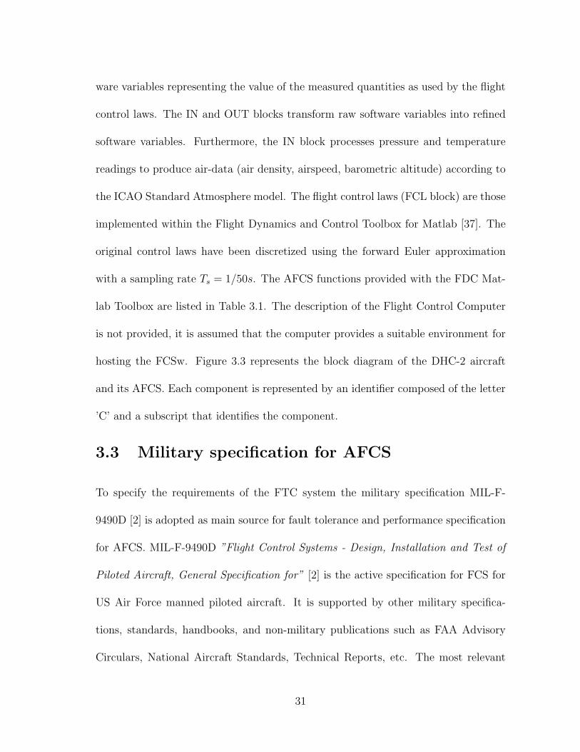
ware variables representing the value of the measured quantities as used by the flight
control laws. The IN and OUT blocks transform raw software variables into refined
software variables. Furthermore, the IN block processes pressure and temperature
readings to produce air-data (air density, airspeed, barometric altitude) according to
the ICAO Standard Atmosphere model. The flight control laws (FCL block) are those
implemented within the Flight Dynamics and Control Toolbox for Matlab [37]. The
original control laws have been discretized using the forward Euler approximation
with a sampling rate Ts = 1/50s. The AFCS functions provided with the FDC Mat-
lab Toolbox are listed in Table 3.1. The description of the Flight Control Computer
is not provided, it is assumed that the computer provides a suitable environment for
hosting the FCSw. Figure 3.3 represents the block diagram of the DHC-2 aircraft
and its AFCS. Each component is represented by an identifier composed of the letter
’C’ and a subscript that identifies the component.
3.3 Military specification for AFCS
To specify the requirements of the FTC system the military specification MIL-F-
9490D [2] is adopted as main source for fault tolerance and performance specification
for AFCS. MIL-F-9490D ”Flight Control Systems - Design, Installation and Test of
Piloted Aircraft, General Specification for” [2] is the active specification for FCS for
US Air Force manned piloted aircraft. It is supported by other military specifica-
tions, standards, handbooks, and non-military publications such as FAA Advisory
Circulars, National Aircraft Standards, Technical Reports, etc. The most relevant
31

CADC
CDAC
CPAH CALH
CRAH CHH CHS
CCP
Cout
Airframe����
controlsurfaces����engine
DHC-2 Aircraft
Cin
CDAC
CADC
CPAH CALH
CRAH CHH CHS
FCL
��������Cp Cq Cr CT Cps
Cqdyn Cψ Cθ Cφ����CAx CAy
CAz Cα
Sp Ss
CCP����CAIL
CELV
CRUD
ACT
FCSwFCC
Cin
AFCS
Cout
Figure 3.3: Block diagram of DHC-2 aircraft and its FCS.
32

supporting documents with respect to this research is the military specification MIL-
F-8785C ”Flying Qualities of Piloted Airplanes” [4], the supplement ”Appendix to
Background Information and User Guide for MIL-F-9490D” [3], and the Technical
Reports ”Background Information and User guide for MIL-F-9490D” [1] and ”Back-
ground Information and User guide for MIL-F-8785C” [5].
MIL-F-9490D contains FCS requirements specification (Section 3) along with clas-
sification of FCS operational states and of FCS criticality (Section 1), and quality
assurance procedures (Section 4). In fact, the document is structured to serve as a
guide for all aspects of design, analysis, and test of FCS. The requirements specifi-
cation spans over the whole system hierarchy, from high-level system requirements
(Section 3.1) to subsystem and components requirements (Section 3.2). It covers a
wide typology of requirements such as performance requirements for autopilot func-
tions, automatic navigation, ride smoothing, etc.; functional requirements for failure
immunity, system test and monitoring, AFCS override, warning and status annun-
ciations, etc.; structural requirements; maintenance requirements; implementation
requirements related to technical details such as wiring, shielding, assembling, etc.
For the purpose of developing the requirements specification for the FTC system a
narrow subset of requirements has been selected. Appendix B.1 contains the referred
military specifications. Selected specifications are reported as they are, with modi-
fications and cuts according to the scope indicated in the sequel. The performance
requirements for the following autopilot functions are considered: Pitch Attitude
Hold (PAH), Altitude Hold, (ALH), Roll Attitude Hold (RAH), Heading Hold (HH),
33
and Heading Select (HS). Coordination requirements for lateral-directional control
functions, both in steady banked turns and in level flight are considered. Among
the functional requirements the focus is on fault-tolerance requirement, limited to
those relevant to fail-operational functions. Failure transient requirements are not
considered since the focus is on fail-operational capability only.
Specifications contained in [2] do not constitute the whole set of specification for
an aircraft; rather, they represent the aircraft-independent specifications. Aircraft-
dependent specifications are collected within the documentation provided by the air-
craft manufacturer and are referred to as detail-specifications. They specify the op-
erational envelope of the aircraft, the aircraft normal and fault states, the maneuver
limits, AFCS functions and their operation such as engagement and disengagement
procedures, selection logic, functional safety criteria and limits, and all relevant in-
formation related to the specific aircraft. To develop the DHC-2 detail-specification
the documentation discussed in the previous section is adopted.
34

Chapter 4
Formal specification of the FTCenvironment
The FTC specification is developed on top of the performance specification derived
from MIL-F-9490D and of the DHC-2 detail-specification. Since the objective is
to develop a formal requirements specification for the FTC, performance and detail
specification needs to be formalized first. Relational algebra is adopted as the formal
specification framework. It is introduced in Section 4.1; for a more detailed descrip-
tion of relational algebra refer to Appendix A and therein referenced bibliography.
To develop the performance and detail formal specification the relevant requirements
are decomposed on a functional basis into elementary requirements. Each elementary
requirement is formalized separately to produce an elementary specification. Then,
composition operators of relational algebra are used to build up higher level require-
ments to develop the whole specification. In this chapter the approach toward formal-
izing the elementary requirements is described in detail. The formalization process is
illustrated on one of the elementary requirements from the performance specification.
Then, the composition of the elementary specifications is shown using an example.
Finally, the requirement structure of the performance and detail specification are
35
illustrated.
4.1 Relational specification of elementary require-
ments
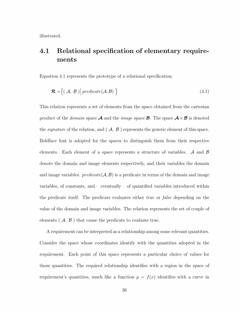
Equation 4.1 represents the prototype of a relational specification.
R ={( A, B )
∣∣∣ predicate(A,B)}
(4.1)
This relation represents a set of elements from the space obtained from the cartesian
product of the domain space A and the image space B. The space A×B is denoted
the signature of the relation, and ( A, B ) represents the generic element of this space.
Boldface font is adopted for the spaces to distinguish them from their respective
elements. Each element of a space represents a structure of variables. A and B
denote the domain and image elements respectively, and their variables the domain
and image variables. predicate(A,B) is a predicate in terms of the domain and image
variables, of constants, and – eventually – of quantified variables introduced within
the predicate itself. The predicate evaluates either true or false depending on the
value of the domain and image variables. The relation represents the set of couple of
elements ( A, B ) that cause the predicate to evaluate true.
A requirement can be interpreted as a relationship among some relevant quantities.
Consider the space whose coordinates identify with the quantities adopted in the
requirement. Each point of this space represents a particular choice of values for
those quantities. The required relationship identifies with a region in the space of
requirement’s quantities, much like a function y = f(x) identifies with a curve in
36

the space X × Y . This region contains all the elements whose quantities’ values
satisfy the required relationship. A relation of the type described in equation 4.1
can identify that region – hence specify the related requirement – provided that the
adopted constants and variables represent the relevant quantities, and the predicate
captures the required relationship among those quantities.
In the requirement formalization process the quantities that are explicitly or im-
plicitly used to formulate the requirement are identified first. Hence, constants and
variables to represent those quantities are introduced. Constants are used to rep-
resent fixed quantities; image variables are used to represent quantities whose value
is somehow constrained by the requirement; domain variables are used to represent
quantities whose value delimits the scope of the requirement; quantified variables are
used to represent quantities that play a role in the formulation of the requirement
but that are neither constrained, nor used to specify the requirements scope. For
the purpose of making the relation more readable and the whole specification less
repetitive and cumbersome auxiliary terms are introduced. These terms represent
expressions and functions that are repetitively used within the specification. Finally,
a predicate that captures the semantics of the requirement is formulated. This re-
quires the predicate to evaluate true if and only if the required relationship among
the requirement quantities holds.
Typically, variables used in relations represent the instantaneous value of the
related quantities. This approach allows for specifying requirements in terms of in-
stantaneous input/output relationships, but it is not suitable for specifying AFCS
37
requirements. Most of AFCS performance requirements are formulated as a con-
straint over a quantity’s time evolution within a certain time interval, rather than
over the quantity’s instantaneous values. Damping requirements, and RMS-deviation
requirements are among two examples. The damping requirement is typically ex-
pressed in terms of the damping factor of the equivalent second order system. To
verify this requirement an identification procedure is used to process system input
and output over the relevant time interval and to produce the equivalent system. It
is not possible to formulate the damping requirement on the basis of instantaneous
input/output values. The RMS-deviation requirement is by definition a constraint
over the integral of the output within the relevant time interval. Once again, this
requirement cannot be formulated as a constraint over instantaneous values of system
output.
To solve this problem the author adopts variables that represent the whole time
evolution of the related quantity, rather than its instantaneous values. For example,
the variable φ() is used to represent the time evolution of the bank angle within the
time interval [0,∞). The empty brackets () are adopted to indicate that the variable
represents the whole time evolution of a quantity rather than the value of the quantity
at a specific time instant.
To illustrate the requirements formalization process and provide a guide to inter-
preting the relational specification the formalization of the Heading Hold (HH) control
function requirement is commented. This requirement is fairly simple, yet provides a
number of meaningful points for discussion. The plain-English specification from [2]
38

is reported below; to facilitate the analysis each section of the requirement has been
labeled with a letter.
3.1.2.2 Heading Hold
a) In smooth air, heading shall be maintained within a static accuracy of ±0.5
degree with respect to the reference.
b) In turbulence, RMS deviations shall not exceed 5 degrees in heading at the
intensities specified in 3.1.3.7.
c) When heading hold is engaged, the aircraft shall roll towards wings level.
d) The reference heading shall be that heading that exists when the aircraft passes
through a roll attitude that is wings level plus or minus a tolerance.
As first step the plain-English requirement is analyzed to identify the quantities
that are used either explicitly or implicitly within the specification. During this
analysis the author introduces – sometimes between brackets – the identifiers that
will represent those quantities within the relation. The HH requirement specifies
accuracy requirements for the heading angle (ψ()) for operation in both smooth air
and turbulence when the HH function is engaged. Hence, the two operation cases must
be separated. To this purpose the auxiliary function turb(ta, tb)is introduced. This
predicate is expressed in terms of the random and discrete turbulence components
of the wind velocity vector uwt(), vwt(), wwt(), uwg(), vwg(), wwg(), and of the time
instants ta and tb. It returns false if and only if the airplane is operating in smooth air
within the time interval [ta, tb]. Accuracy requirement for operation in turbulence are
expressed in terms of the RMS deviation from the reference heading. The auxiliary
39
function RMS(dev(), ta, tb) is introduced; it returns the RMS value of the variable
dev() within the specified time interval [ta, tb]. The relevant time instants of the
specification are three. The first one (t1) is the HH function engagement instant. The
second one (t2) is the time instant when the reference heading (ψr) is determined.
In fact, the specification requires the airplane to roll (φ()) towards wings level, and
fixes the reference heading as ”that heading that exists when the aircraft passes trough
a roll attitude that is wings level plus or minus a tolerance” (φacc). The third time
instant (t3) can be any time instant preceding HH function disengagement. Other
quantities that need to be represented are the required accuracy levels in both smooth
air (ψacc) and turbulence (ψRMS) operation, and the HH control switch (SWHH()).
Another auxiliary function is introduced: engaged(SW (), ta, tb); it returns true if
control SW () is engaged at t = ta and stays engaged within the whole time interval
[ta, tb].
After identifying the relevant quantities the related identifiers are separated into
classes of constants, domain, image, and quantified variables, and auxiliary functions.
Tables 4.1 trough 4.4 list all identifiers used within the HH relational specification.
The signature and the predicate of the HH relational requirement are given by
the following two equations:
HHsign =(( SWHH(), uwt(), vwt(), wwt() ), ( ψ(), φ() )
)(4.2)
40

Table 4.1: Constants used within the specification of the HH function.
ID and value Type Definition
ψacc = 0.5 · degree2SI angle-T heading accuracy in smooth airψRMS = 5 · degree2SI angle-T RMS heading accuracy in turbulenceφacc = 1.0 · degree2SI angle-T roll accuracy in smooth air
Table 4.2: Domain and image variables used within the specification of the HH func-tion.ID Type Definition
SWHH() time-T → switch-T HH autopilot on/off switchuwt(), vwt(), wwt() time-T → velocity-T wind-turbulence components of wind
velocity along body-axesuwg(), vwg(), wwg() time-T → velocity-T wind-gust components of wind veloc-
ity along body-axesψ() time-T → angle-T heading angleφ() time-T → angle-T bank angle
Table 4.3: Quantified variables used within the specification of the HH function.
ID Type Definition
t time-T generic time instantt1 time-T HH function engagement time instantt2 time-T time instant when the reference heading is determinedt3 time-T time instant delimiting the scope of the requirementψr angle-T reference heading
Table 4.4: Predicates and functions used within the specification of the HH function.
ID Description
engaged(SW (), ta, tb) predicate that evaluates true only if the switch SW () isengaged at t = ta and stays engaged throughout the timeinterval [ta, tb]
RMS(f(), ta, tb) Root Mean Square value of the function f() over the timeinterval [ta, tb]
turb(ta, tb) predicate that evaluates true if random and discrete turbu-lence wind components are not zero
41
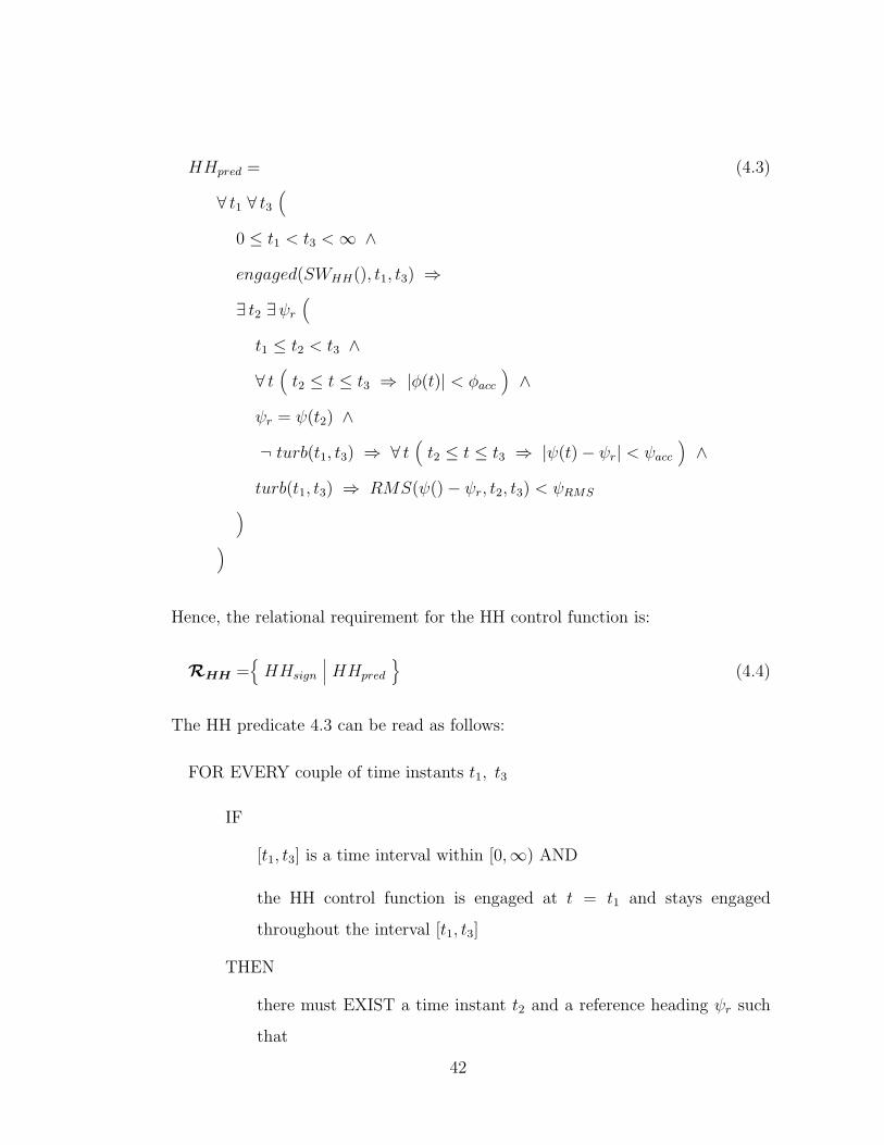
HHpred = (4.3)
∀ t1 ∀ t3(
0 ≤ t1 < t3 < ∞ ∧engaged(SWHH(), t1, t3) ⇒∃ t2 ∃ψr
(t1 ≤ t2 < t3 ∧∀ t
(t2 ≤ t ≤ t3 ⇒ |φ(t)| < φacc
)∧
ψr = ψ(t2) ∧¬ turb(t1, t3) ⇒ ∀ t
(t2 ≤ t ≤ t3 ⇒ |ψ(t) − ψr| < ψacc
)∧
turb(t1, t3) ⇒ RMS(ψ() − ψr, t2, t3) < ψRMS))
Hence, the relational requirement for the HH control function is:
RHH ={
HHsign
∣∣∣ HHpred
}(4.4)
The HH predicate 4.3 can be read as follows:
FOR EVERY couple of time instants t1, t3
IF
[t1, t3] is a time interval within [0,∞) AND
the HH control function is engaged at t = t1 and stays engaged
throughout the interval [t1, t3]
THEN
there must EXIST a time instant t2 and a reference heading ψr such
that
42
c1) t2 is within the interval [t1, t3) AND
c2) the bank angle is approximately zero within the time interval
[t2, t3) AND
d) the reference heading ψr is the heading angle at t = t2 AND
a) IF there is no turbulence within the time interval [t1, t3] THEN
the deviation of the heading angle ψ from the referenced heading
ψr shall not be larger than ψacc at all time instants within the time
interval [t2, t3] AND
b) IF there is turbulence within the time interval [t1, t3] THEN the
RMS value of the deviation of the heading angle ψ from the refer-
enced heading ψr over the time interval [t2, t3] shall not be larger
than ψRMS
The labels in the THEN section recall the labels inserted in the plain-English
specification.Sections a) and b) refer to the accuracy requirement in smooth and
turbulence operation respectively. Both sections c1) and c2) refer to section c) of the
plain-English specification. This section reads ”When heading hold is engaged the
aircraft shall roll towards wings level”. This section has been formalized by requiring
the airplane to reach – at a certain time instant t2 – a state with a bank angle close to
zero. To quantify how close, the author adopted the accuracy threshold φacc used in
the Roll Attitude Hold (RAH) specification ( Section 3.1.2.1 of [2], see also Appendix
B.1). This solution is the author’s best guess to make up for the lack of a threshold
in the plain-English specification. The same solution was adopted to make up for
the lack of indications on how to determine the reference heading. In fact, section d)
43
of the original specification reads ”The reference heading shall be that heading that
exists when the aircraft passes through a roll attitude that is wings level plus or minus
a tolerance”. The tolerance is left unspecified. Another problem within the plain-
English specification is the lack of a settling-time requirement for the airplane to reach
wings level. Unfortunately, the settling-time requirement cannot be extracted from
the RAH specification since in that specification the settling-time is specified only for
the case of a 5 degree attitude disturbance.
While analyzing the AFCS requirements from [2] the author found out that most
of them are incomplete and not properly specified. The qualitative nature of the
AFCS specification is explicitly stated in Section 3.1.11 of [4]. The qualitative na-
ture of some requirements like ”Entry and exit from the turn shall be smooth and
rapid” (Section 3.1.2.3 in [2]), ”For engagement at rates above 2000 fpm the AFCS
shall not cause any unsafe maneuvers” (Section 3.1.2.5 in [2]), or ”No out of trim
condition shall exist at disengagement which cannot be easily controlled by the pi-
lot” (Section 3.1.3.3.2 in [2]) did not allow to develop a formal specification for the
whole plain-English requirement. However, this does not represent a problem for
the development of the FTC formal specification. Because of the monotonic nature
of relational requirements, the FTC specification can be developed on top of tem-
porary FCS specification, postponing completion of the FCS specification to a later
refinement step.
44

4.2 Composition of elementary requirements
In order to describe the composition of the elementary specifications the composi-
tion operators of relational algebra are now introduced along with the concept of
refinement ordering between requirements and of system correctness. Relation R1
refines relation R2, denoted by R1 w R2, if R1 specifies a stronger requirement
than R2, in the sense that it imposes a constraint over a wider domain and/or it is
more specific. System correctness is defined as a refinement constraint between the
relation P representing the system implementation and the relation R representing
the system requirements: P is correct with respect to R if P w R. The adopted
composition operators are the join ( t ) and the product (◦) operators. The join of
two relations represents the sum of the requirements. A system P that meets the
requirement specified by R1 t R2 also meets the requirements specified by R1 and
R2 separately. This is formally stated by the following formula:
P w R1 t R2 ⇒ P w R1 ∧ P w R2 (4.5)
The join operator is adopted to compose relations that capture parallel requirements
within the specification structure. The product of two relations R1 and R2 represents
the requirement of the sequence of two systems P1 and P2 whose requirements are
specified by R1 and R2 respectively. If P12 denotes the series of systems P1 and P2
the main property of the product operator is defined by the following formula:
P1 w R1 ∧ P2 w R2 ⇔ P12 w R1 ◦ R2 (4.6)
45
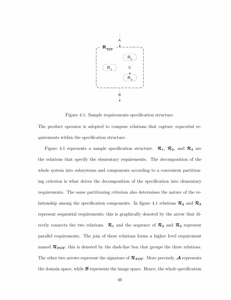
C
R3
A
B
R2
R1
RTOT
Figure 4.1: Sample requirements specification structure.
The product operator is adopted to compose relations that capture sequential re-
quirements within the specification structure.
Figure 4.1 represents a sample specification structure. R1, R2, and R3 are
the relations that specify the elementary requirements. The decomposition of the
whole system into subsystems and components according to a convenient partition-
ing criterion is what drives the decomposition of the specification into elementary
requirements. The same partitioning criterion also determines the nature of the re-
lationship among the specification components. In figure 4.1 relations R2 and R3
represent sequential requirements; this is graphically denoted by the arrow that di-
rectly connects the two relations. R1 and the sequence of R2 and R3 represent
parallel requirements. The join of these relations forms a higher level requirement
named RTOT ; this is denoted by the dash-line box that groups the three relations.
The other two arrows represent the signature of RTOT . More precisely, A represents
the domain space, while B represents the image space. Hence, the whole specification
46
can be formulated as follows:
R1 ⊆ A × B (4.7)
R2 ⊆ A × C (4.8)
R3 ⊆ C × B (4.9)
RTOT = R1 t R2 ◦ R3 (4.10)
Composition operators cannot be applied to any couple of relations. The join
operator can be applied only to relations with the same signature. On the other
hand, the product operator can be applied only if the image space of the left re-
lational operand coincides with the domain space of the right relational operand.
Hence, before composing the relations to form higher level requirements the domain
and/or the image spaces of the relations used in the composition might need to be
expanded. Since, the expansion operation preserves the property that is captured
by the relation, the expanded relation specifies the same requirement as the original
relation. A possible approach is to expand the spaces of all relations to the space of
all variables that appear in the specification. The expanded relations would form a
set of homogeneous relations and both join and product operators could be applied
to any couple of expanded relations. However, this approach would lead to a flat set
of relations, where the structure of the system is lost.
The adopted expansion approach preserves the structure of the system, with the
result of a more informative specification that potentially leads to a more effective
validation. To illustrate the expansion process the composition of the Heading Hold (
Section 3.1.2.2 in [2]) and the Heading Select (HS) ( Section 3.1.2.3 in [2]) requirements
47

is illustrated. For the expansion operation only the two relation signatures are needed.
The signature of the HH relation is given in equation 4.2. The signature of the HS
relation from the plain-English requirement is now determined.
3.1.2.3 Heading Select
a) The aircraft shall automatically turn through the smallest angle
b) to any heading selected or preselected by the pilot and
c) maintain that heading to the tolerances specified for heading hold.
d) The contractor shall determine a bank angle limit which provides a satisfactory
turn rate and precludes impending stall.
e) The aircraft shall not overshoot the selected heading by more than 1.5 degrees.
f) Entry into and exit from the turn shall be smooth and rapid.
g) The roll rate shall not exceed 10 deg/sec and
h) roll acceleration shall not exceed 5 deg/sec/sec.
The requirement imposes a constrain over the roll angle φ() (section a), over the
heading angle psi() (sections c and e), and over the roll rate p()(sections g and h). The
scope of the requirement is determined by the HS engagement control switch SWHS()
(implicitly assumed activated), by the selected reference heading ψr() (section b), and
by the wind velocity components uwt(), vwt(), wwt() (section c) through the reference
to the HH requirement. Hence, the signature for the HS relational requirement is:
HSsign =(( SWHS(), ψr(), uwt(), vwt(), wwt() ), ( ψ(), φ(), p() )
)(4.11)
48
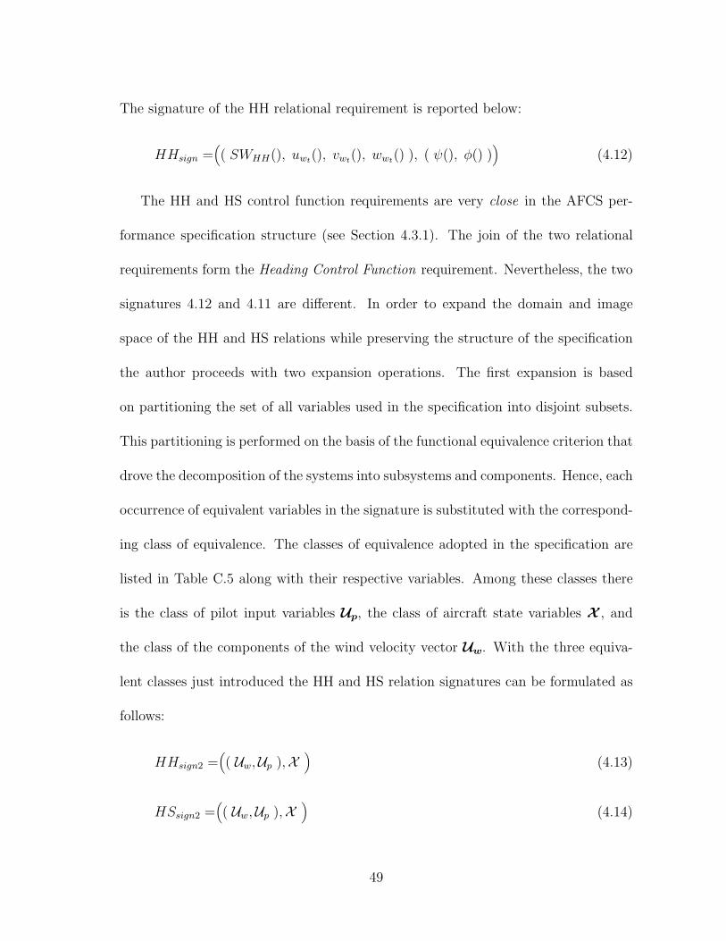
The signature of the HH relational requirement is reported below:
HHsign =(( SWHH(), uwt(), vwt(), wwt() ), ( ψ(), φ() )
)(4.12)
The HH and HS control function requirements are very close in the AFCS per-
formance specification structure (see Section 4.3.1). The join of the two relational
requirements form the Heading Control Function requirement. Nevertheless, the two
signatures 4.12 and 4.11 are different. In order to expand the domain and image
space of the HH and HS relations while preserving the structure of the specification
the author proceeds with two expansion operations. The first expansion is based
on partitioning the set of all variables used in the specification into disjoint subsets.
This partitioning is performed on the basis of the functional equivalence criterion that
drove the decomposition of the systems into subsystems and components. Hence, each
occurrence of equivalent variables in the signature is substituted with the correspond-
ing class of equivalence. The classes of equivalence adopted in the specification are
listed in Table C.5 along with their respective variables. Among these classes there
is the class of pilot input variables Up, the class of aircraft state variables X , and
the class of the components of the wind velocity vector Uw. With the three equiva-
lent classes just introduced the HH and HS relation signatures can be formulated as
follows:
HHsign2 =(( Uw,Up ),X
)(4.13)
HSsign2 =(( Uw,Up ),X
)(4.14)
49
The two signatures 4.13 and 4.14 are now the same and the two relations can be
joined.
For some relations a second expansion operation is needed. This is the case of the
sensor requirement RSp and of the control panel requirement RCP in the DHC-2
detail-specification. The two requirements need to be joined as part of the computer
input requirement RCIN. However, they have the following different signatures after
the first expansion:
RSsign2 =(X , X
)(4.15)
RCP sign2 =(Up, Up
)(4.16)
X and Up represent the class of electrical signals correlated to aircraft states and
pilot inputs respectively. The problem arises because the equivalence partitioning
introduced in the first expansion is based on the first subsystem composition of the
FTC environment components. The RCIN relation is one level above, since it sums
the subsystem requirements RSp and RCP . To solve this problem equivalent classes
that are at the same hierarchical level in one of the successive compositions of the
system components are merged together. Hence, X and Up, and X and Up are
combined to form the following common signature for RSp and RCP :
RSsign2 =(( X ,Up ), ( X , Up )
)(4.17)
Table C.1 collects the original signature and the expanded signatures for each rela-
tional term used in the specification.
50

4.3 Formal specification of the FTC environment
Appendix B collects the elementary relational specifications of the FTC environment.
More specifically, Section B.1 collects the elementary requirements of the AFCS per-
formance specification, Section B.2 collects the elementary requirements of the DHC-2
detail-specification, Section B.3 collects the fault modes for each fallible component
of the FTC environment, and Section B.4 collects the restriction sets used to delimit
the scope of the AFCS specification when applied to the DHC-2 airplane.
Each relational requirement is denoted by the letter R and a subscript that iden-
tifies the specific requirement (e.g. RPAH identifies the relational requirement for
the PAH control function). Each requirement is formalized as illustrated in Section
4.1. The signature reported within the definition of the relation is the signature ob-
tained after the first expansion discussed in the previous section. Table C.1 collects
all elementary requirements along with a short explanation of the property captured
by the relation, domain and image variables, and the signatures obtained after each
expansion. The composition of the elementary specifications to form the performance
and detail specification are discussed in the sections 4.3.1 and 4.3.2.
Airplane failure states are part of the DHC-2 detail-specification. Each airplane
failure state consists of the airplane normal state modified by one or more malfunc-
tions in airplane components or systems. Each mode of failure that is not extremely
remote should be considered (see Section 3.1.6.2 of [4]). The specification of the
detailed set of airplane failure states is out of the scope of this research. Hence,
only one fault-mode for each fallible component is specified. Relations are used to
51

describe classes of fault-modes for a specific component. For example, the relation
specifying the partial loss of rudder control surface models any partial loss up to total
loss of the surface. The identifier of a fault-mode relation is the same as that used
for the relation describing the required behaviour of the corresponding component,
with a number added to the subscript to identify the fault mode (e.g. Rp,1 is the
relation describing fault mode number 1 for the roll rate gyro). The signature of a
fault-mode relation is the same used in the relation specifying the requirements for
the corresponding component, while the related predicate captures the specific faulty
behaviour. The considered faults are very simple: these are partial loss of rudder con-
trol surface, engine loss, bad connection of sensor output, and stuck actuators. Sensor
fault modes are an extrapolation of results from fault-mode-tests performed on rate
gyros similar to the gyros adopted in this specification. For lack of aerodynamic data
failure of a single aileron or a of single elevator are not modeled. Section B.3 collects
all fault-mode relations, while Table C.3 lists them along with a brief description.
The restriction-sets are used to delimit the scope of the performance specifi-
cation. There are three restriction-sets: Sao, Sat, and SCtr . Sao specifies the
control-function selection logic; this information constitutes part of the airplane
detail-specification as required in Section 3.1.2 of [2]. Sat specifies the turbulence
model to be adopted for verifying performance requirements with the airplane oper-
ating in turbulence. Only random turbulence is considered, while discrete turbulence
(e.g. wind-gusts) and mean wind are not modeled. Effects of wind-shear are omit-
ted since they become dominant in terminal flight-phases, while here the focus is on
52

autopilot functions that are engaged in non-terminal flight-phases only. The model
adopted for random turbulence is the Dryden model with length and intensities scales
as specified in Section 3.7 of [4]. SCtr represents the constraint over trim condition
to guarantee a valid set of values. Each of these sets contains only a subset of the
variables used within the performance specification. To make these sets homogeneous
with the spaces of the relations they are going to be used with they are expanded
as illustrated in Section 4.2. Table B.4 lists the restriction-sets along with a short
description, the relevant variables, and the expanded spaces.
Appendix C collects all supporting tables for the FTC environment specification.
Some of these tables have been already introduced, such as Table C.1 listing the
elementary requirements of the FTC environment, Table C.3 listing the fault-mode
relations, and Table C.4 listing the restriction sets used within the AFCS performance
specification. Table C.2 lists the composed relations used within the performance
and the detail specification along with domain and image spaces. Table C.5 lists
all the classes of equivalent variables obtained with the first expansion discussed in
Section 4.2 along with the set of variables belonging to each class. Table C.6 lists all
domain and image variables used within the relational specification along with their
data-type and a brief description of the represented quantities. Table C.7 defines
the type and value of all the constants used within the specification. Table C.8
lists all quantified variables used within the specification along with their data-type.
Table C.9 defines all the auxiliary terms, functions, and predicates. Finally, Table
C.10 defines all the data-types. SI unit and range of allowed values is specified for
53

each data-type; this information can be used within the validation process to check
requirement consistency. Value range is used to capture indicative constraint over
requirement variables. For example, ranges for airspeed, altitude, and angle of attack
are specified to capture the envelope of validity of the aerodynamic model of the
airplane. Analogously, the rudderDeflection-T type specifies minimum and maximum
deflection of the rudder; bankReference-T and pitchReference-T types specify the
minimum and maximum values of bank and pitch reference angles as specified by the
AFCS designer. Whenever strong typing of variables or constants would result in an
excess of notation or in a cumbersome representation of data we omitted specification
of type or the a looser form of typing was adopted where ranges and units are not
specified. This is for example the case of the matrices of the actuator models in Table
C.7 and of the stabilityDerivative-T and controlDerivative-T types in Table C.10.
4.3.1 Performance requirement composition
Section B.1 collects the elementary requirements for the AFCS performance speci-
fication. Of the performance specification for AFCS the author selected only those
related to static accuracy for operation in smooth air and in turbulence that apply to
the DHC-2 autopilot functions. These are the performance requirements for the PAH,
ALH, RAH, HH, and HS autopilot functions, and the coordination requirements for
lateral-directional control functions, both in Steady Banked Turn (SBT) and in Level
Flight (LF). The original text of the requirements from [2] is reported along with the
relational specification. An intermediate formulation of the requirement bridges the
gap between the two specifications as illustrated in Section 4.1 for the HH function
54
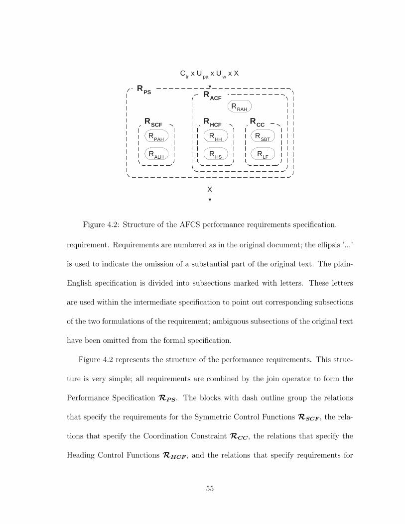
Ctr x U
pa x U
w x X
X
RPAH
RALH
RSCF
RRAH
RHH
RSBT
RLFRHS
RHCF RCC
RACF
RPS
Figure 4.2: Structure of the AFCS performance requirements specification.
requirement. Requirements are numbered as in the original document; the ellipsis ’...’
is used to indicate the omission of a substantial part of the original text. The plain-
English specification is divided into subsections marked with letters. These letters
are used within the intermediate specification to point out corresponding subsections
of the two formulations of the requirement; ambiguous subsections of the original text
have been omitted from the formal specification.
Figure 4.2 represents the structure of the performance requirements. This struc-
ture is very simple; all requirements are combined by the join operator to form the
Performance Specification RPS. The blocks with dash outline group the relations
that specify the requirements for the Symmetric Control Functions RSCF , the rela-
tions that specify the Coordination Constraint RCC, the relations that specify the
Heading Control Functions RHCF , and the relations that specify requirements for
55

the Asymmetric Control Functions RACF . The performance specification RPS is a
relation over the domain space Ctr+Upa+X+Uw and the image space X . These are
the expanded spaces that represent the class of trim-variables Ctr, the class of AFCS
input variables Upa , the class of air-turbulence variables Uw, and the class of airplane
state variables X . Each requirement is expressed as a constraint over the evolution
of the airplane state under specified turbulence conditions, for a specific AFCS input
and trim condition.
The composition of the relations specifying the elementary performance require-
ments is straightforward; all requirements are combined through the join operator
to form the performance specification. The resulting requirement is restricted to the
admissible combination of AFCS inputs, to a valid set of trim-conditions, and to the
required model of wind turbulence by means of the pre-restriction sets introduced in
the previous section. The composition is expressed by the following equations:
SPS = SCtr
⋂ Sao
⋂ Sat (4.18)
RPS = SPS\(
RPAH t RALH t (4.19)
RRAH t RHH t RHS t RSBT t RLF
)4.3.2 DHC-2 detail-specification
Section B.2 collects the elementary requirements for the DHC-2 detail-specification.
These relations specify the required behaviour of each component of the DHC-2 air-
plane and its AFCS. Since most of this information is in terms of analytical equations
describing the operation of the corresponding component there is no plain-English
56

specification counterpart.
Elementary specifications are grouped into different subsections according to their
role within the specification structure. Section B.2.1 collects relations that specify
the airplane dynamics through force RFeq, moment RMeq, kinematic RKeq, and
navigation RNeq equations. The forcing terms for these equations are aerodynamics
forces Raef and moments Raem exerted by the airframe, forces Rcsf and moments
Rcsm exerted by the control surfaces, forces Rpf and moments Rpm exerted by
the engine, and gravity Rgrf and wind Rwf forces. This section also includes the
relations that specify air-data quantities Rad and kinematic acceleration at crew
station Rka. Section B.2.2 collects relations that specify the requirements for the
hardware components of the DHC-2 AFCS. These include actuator specifications
Rrud, Rail, and Relv, all sensor specifications Rp, Rq, Rr, etc. control panel
specification RCP , and FCC interface card specifications RADC, and RDAC. Section
B.2.3 collects relations that specify the requirements for the components of the FCSw.
These are the interface modules Rin and Rout and all the modules related to the
FCL: RPAH
, RALH
, RRAH
, RHS
, and RHH
.
Figure 4.3 illustrates the structure of the detail-specification. This structure is
similar to the block diagram in figure 3.3. The main difference consists in the ex-
pansion of the airplane system into the relations that describe its dynamics. The
display panel has been removed from the AFCS since it is not used within the speci-
fication. The diagram also displays the classes of variables over which these relations
are defined. Some of these classes have been already introduced; some other classes
57

RADCRDAC
RinUpa + XUc
RCP
Upa + X
Uc X
Cm Cf + X
~ ~
^ ^ ^
RFCSw
RFCC
RAFCS
RDHC-2
RCin
Rout
Uc Upa + X- --
Uc
~
��Rcsm
��Rpm
RaemRm
Raef
��Rcsf
��Rpf
Rf
����
RAIL
��RELV
����RRUD
RACT
RFCL
RALH
RPAH
RRAH
RHH
��
Rp����
Rq����
Rr
����Rqdyn��Rθ
����Rps ����RT�Rψ
��Rφ
RSp��
RAx
����RAy
�RAz
��Rα
RSs
Uw + U pm + X
Upa
RHS
Ctr
X
RFeq
Rgrf
Rwf
RMeq
RNeq
RKeq
Rka
Rad
RADC
Rin
RDAC
Figure 4.3: Structure of the DHC-2 detail-specification.
58

are introduced here for the first time. This is the case of the class of the MFCS
control inputs Upm, the class of force and moment aerodynamic coefficients Cf and
Cm, and the class of control surface deflection variables Uc. Identifiers provided of a
mathematical accent (hat, tilde, bar) represent quantities correlated to the quantity
represented by the identifier without accent. The tilde accent is adopted for variables
representing electrical signals, the bar accent is adopted for variables representing the
ADC or DAC software representation of the quantity, and the hat accent is adopted
for software variables. Hence, X is the class of variables representing electrical sig-
nals correlated to the airplane states, X is the class of variables representing ADC
software representation of the airplane states, and X is the class of software variables
representing the airplane states. Similar interpretations hold for the other accented
classes and variables.
With the support of the specification structure in figure 4.3 the elementary re-
quirements of Section B.2 can be composed to form the DHC-2 detail-specification.
This specification is divided into the description of the DHC-2 airplane dynamics
RDHC2 and the DHC-2 AFCS RAFCS. Some relations are introduced to collect
functionally related specifications. These are the relations Rf and Rm that collect
respectively force and moment components involved in the flight dynamics equations,
the relations RSp and RSs that represent the subsystem of primary and secondary
sensors respectively, the relation RFCL that collects the flight control laws, the re-
lation RACT that collects the actuators, the relation RFCSw that represents the
flight control software, and the RFCC that represents the flight control computer.
59

The formal composition of the elementary requirements is expressed by the following
equations
Rf = Raef t Rgrf t Rcsf t Rpf t Rwf (4.20)
Rm = Raem t Rcsm t Rpm (4.21)
RDHC2 = Rf ◦ RFeq t Rm◦ RMeq t RKeq (4.22)
t RNeq t Rad t Rka
RSp = Rp t Rq t Rr t Rψ t Rθ t Rφ (4.23)
t Rps t Rqdynt RT
RSs = RAx t RAy t RAz t Rα (4.24)
RFCL = RPAH
t RALH
t RRAH
t RHH
t RHS
(4.25)
RACT = Rail t Relv t Rrud (4.26)
RFCSw = Rin◦ RFCL◦ Rout (4.27)
RFCC = RADC ◦ RFCSw◦ RDAC (4.28)
RAFCS =(
RSp t RSs t RCP
)◦RFCC ◦ RACT (4.29)
4.3.3 Correctness of AFCS design
The AFCS performance specification RPS represents the system requirements for
an AFCS in terms of required behaviour of the airplane when equipped with the
AFCS. The DHC-2 detail-specification and the AFCS performance specification can
be composed as follows to form the specification of the airplane equipped with the
AFCS:
60
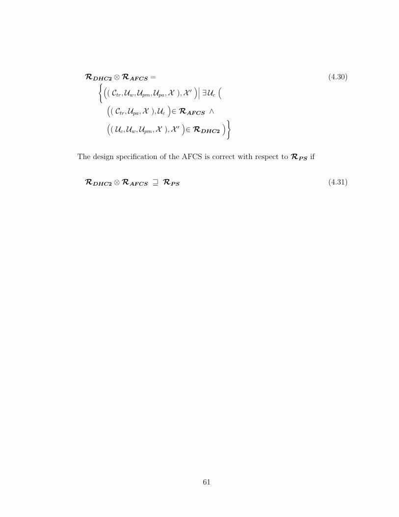
RDHC2 ⊗ RAFCS = (4.30){(( Ctr,Uw,Upm,Upa,X ),X ′
)∣∣∣ ∃Uc
((( Ctr,Upa,X ),Uc
)∈ RAFCS ∧(
( Uc,Uw,Upm,X ),X ′)∈ RDHC2
)}
The design specification of the AFCS is correct with respect to RPS if
RDHC2 ⊗ RAFCS w RPS (4.31)
61

Chapter 5
Formal requirements specificationof the FTC
This chapter contains the formal specification of the FTC system. In the first section
fault tolerance requirements are divided into functional and non-functional require-
ments and formulated in a form that facilitates their formalization. The relational
specification is developed on top of the structured plain-English requirements. In
the second section the focus is on the core of the FTC system, that is the FTC-AR
module. The other FTC modules serve as interface and their formal specifications
are collected in section B.5. The last section illustrates some concepts related to the
feasibility analysis of the fault tolerance requirements.
5.1 FTC requirements
5.1.1 FTC functional requirements
The relation RPS captures the performance specification of the AFCS. If each compo-
nent of the DHC-2 airplane equipped with AFCS satisfies the corresponding require-
ments then the correctness of the design, as formulated by equation 4.31, guarantees
that the actual behaviour of the system satisifies the performance requirements. Fault
62
tolerance requirements aim to guarantee that performance specification are met also
in case one or more of the system components fail to meet the corresponding speci-
fication. The main concepts related to fault tolerance for flight control systems were
introduced in Section 3.1.2. The definition of fail operational and fail passive are
reviewed here in support of the analysis that will lead to the formulation of the fault
tolerance requirements for the AFCS of the DHC-2 airplane:
Fail operational The capability of the FCS for continued operation without degra-
dation following a single failure, and to fail passive in the event of a related
subsequent failure.
Fail passive The capability of the FCS to automatically disconnect and to revert to
a passive state following a failure.
In the definition of fail operational capability the term related subsequent failure
is ambiguous. In the first instance the requirement aims to capture the desired be-
haviour of the fault tolerant system under the condition of single and double failure.
Hence, the temporal sequence in which the failures occur is not relevant. In the second
instance, it is not clear under what conditions two failures are related. In the frame-
work of physical redundancy the failure of two out of three redundant units might
be considered as a case of related failures. However, this definition depends on the
specific approach to achieving fault tolerance and looses its validity in the framework
of analytical redundancy. The author adopts a definition that has a functional basis.
Fallible components are partitioned into the following classes of equivalence: class of
measurement units M, class of actuation units A, class of processing units P , and
class of interface units I . Failures of components that belong to the same class are
63

considered related. This definition captures the author’s best approach-independent
interpretation of the term related failures in the original requirement. The rationale
behind this interpretation is the implicit assumption in the definition of fail opera-
tional capability that the occurrence of two related failures is more critical than the
occurrence of two unrelated failures. In fact, for related failures the fault tolerant
system is required to be fail passive, while for unrelated failures it is required to con-
tinue operation. Failure of components serving the same function is potentially more
critical than failure of components serving different functions. Hence, the component
function is a suitable basis for defining related failures.
Proper formulation of the automatic disengagement requirement as it appears in
the fail passive definition would require the formal description of the MFCS. The
details of the transition from AFCS to MFCS following automatic disengagement are
not considered; the FTC is simply required to signal this transition.
Another requirement for fault tolerant flight control systems is the ”FCS warning
and status annunciation” requirement (section 3.2.1.4.2 of [2]). The FTC is required
to signal a warning in correspondence of a fault and of automatic disengagement.
Hence, the FTC shall have a display panel with a warning light for each monitored
component and an additional light for automatic disengagement. Furthermore, the
FTC control panel shall have a switch to control the ON/OFF status of the FTC
system.
The fail operational capability definition and the warning and status annunciation
requirement represent the core of the fault tolerance requirements specification. To
64

formulate the fault tolerance requirements in a format more suitable to formalization
the following fault hypotheses are introduced:
H0 Fault free hypothesis; all of the components used by the FTFCS are working
according to the corresponding specifications.
H1 Single failure hypothesis; at least one component among those used by the FTFCS
is working according to one of its fault modes, and there are no related faults;
H2 Multiple failure hypothesis; at least two related components used by the FTFCS
are working according to one of the corresponding fault modes.
In the definition of fault hypotheses H1 and H2 the fault modes have been adopted
to specify the behaviour of a component that is not working according to its spec-
ification. The rationale behind this choice is that required behaviour and faulty
behaviours do not necessarily cover all the possible modes of operation of a compo-
nent. Hence, both the required behaviour and the set of fault modes are adopted
as basis for the certification, as opposed to adopting the required behaviour and any
possible behaviour that does not refine the component specification.
The fault tolerance requirements are formulated as follows:
- if the FTC is not engaged then the FTFCS shall operate like the original AFCS
and all FTC warning lights shall be off;
- if the FTC is engaged then
- under conditions captured by the fault hypothesis H0 the DHC-2 airplane
equipped with the FTFCS shall meet the performance specification RPS
and all FTC warning lights shall be off;
65
- under conditions captured by the fault hypothesis H1 the DHC-2 airplane
equipped with the FTFCS shall meet the performance specification RPS
and only the warning lights corresponding to the faulty components shall
be on;
- under conditions captured by the fault hypothesis H2 the FTC automatic-
disengagement warning light shall be on.
5.1.2 FTC non-functional requirements
In Section 3.1.2 two non-functional requirements for the FTC system were introduced.
These requirements were in the form of constraint over the modular architecture of
the solution and over the redundancy approach to be adopted for each component.
According to this last requirement fault tolerance must be achieved by means of
physical or analytical redundancy depending on the nature of the component. Fault
tolerance with respect to failure of components that belongs either to class P or
to class I must be achieved adopting the physical redundancy approach, while fault
tolerance with respect to failure of components of classes M and A must be achieved
adopting the analytical redundancy approach. Furthermore, the solution must be
modular, with the following assigned priority among modules: fault tolerance with
respect to failure of components of class P and I is achieved first, then fault tolerance
with respect to failure of components of class M, and finally fault tolerance with
respect to failure of components of class A. This priority ordering implies that the
failure of components of class P and I is transparent to the module that is required
to provide fault tolerance with respect to failure of components of class M, while the
failure of components of class A is not. For this research the focus is on the FTC
66

module that provides fault tolerance with respect to sensor failures.
The above non-functional contraints have an impact on the specification of the
FTC requirements. The analytical redundancy approach constraint affects the fault
hypothesis definitions. Since analytical redundancy maps into the correlation of sen-
sor outputs and actuator inputs at software level, each failure that might affect such
correlation must be considered; that is, fault hypotheses must be total with respect to
operation of fallible components. The module priority constraint also has an impact
on the definition of the fault hypotheses, since it determines whether a failure should
be considered transparent to the FTC module or not. Furthermore, the modular ap-
proach translates into a shift in the target of the FTC requirements from preserving
AFCS performance specification in case of single failure to preserving functionality of
the set of sensors. The specification of the set of sensors is:
RXX =( RSp t RSs ) ◦RADC ◦ Rin (5.1)
5.1.3 FTC-AR requirements
Figure 5.1 represents the specification structure of the DHC-2 airplane equipped with
the FTFCS. Blocks with a thicker outline represent the components of the FTC
system. The core of the FTC is the FTC-AR module. This is the component required
to exploit analytical redundancy of the DHC-2 system to provide fault tolerance with
respect to sensor failures. The other components of the FTC system are the control
(CP) and display (DP) panels, that serve as interface between the FTC and the pilot,
the hardware (ADC, DAC) and software blocks (IN, OUT) that link the FTC external
interface to the core module FTC-AR, and the FTC-SW block that serves as a switch
67

RADCRDAC
Rin
RCP
Cm Cf + X
RFTFCS
RDHC-2
Rout
S1
Uc+Yf
~
��Rcsm
��Rpm
RaemRm
Rf
����
RAIL
��RELV
����RRUD
RFCL
RALH
RPAH RRAH
RHH
��
Rp
����Rq
����
Rr
����Rqdyn��Rθ
����Rps����RT�Rψ
��Rφ
RSp
�RAx
��RAy
��RAz����
Rα
RSs
Uw + U pm + X
Upa
RHS
Ctr
X
RFTC-CPRFTC-DP
RFTC-DAC RFTC-ADC
RFTC-out RFTC-in
RFTC-AR
RACT RCout
S6
S3S7
S4
S8 RFTC-sw
S2S5
S9
~
Uf
Raef
��R
csf
��R
pf
RFeq
Rgrf Rwf
RMeq
RNeq
RKeq
Rka
Rad
RCin
Rin
RFCSw
RFCC
Uf+U pa+X~ ~~
Uc
X
RADCRDAC
RCP
Cm
S1: U f + U pa + X
S2: U f + U pa + X
S3: U f + X
S4: X
S5: Upa + X'
S6: Uc
S7: Y f
S8: Uc
S9: Y f + U c
- - -
^ ^ ^
^ ^
^
^ ^
^
^
^
- -
Figure 5.1: DHC-2 and FTFCS requirements specification structure.
68

between the original AFCS and the FTFCS. The FTC-SW fulfills a safety function;
if the FTC is disengaged the FTC-SW block isolates the FTC-AR module so that its
output does not affect the input to the FCL. Introduction of the FTC system into
the AFCS leads to the introduction of new quantities used in the formulation of the
requirements. These quantities are represented by the class of FTC input variables
Uf , the class of FTC warning variables Yf , and the class of validated airplane states
X .
With the decomposition of the FTC system into its elementary components the
FTC-AR module has been isolated. This is the FTC module the inherits the fault
tolerance requirements. The FTC-AR requirements are derived from the fault toler-
ance requirements after integrating them with the non-functional constraints and by
projecting them onto its interface. This process leads to the following fault hypothe-
ses:
HM0 Fault free hypothesis;
- all of the sensors used by the FTFCS are working according to the corre-
sponding specifications and
- all of the processing and interface units used by the FTFCS are working
according to the corresponding specifications and
- no more than two actuation units used by the FTFCS are working ac-
cording to one of the corresponding fault modes, while all the others are
working according to the corresponding specification, and
- all fallible components not used by the FTFCS are either working according
to the corresponding specification or according to one of the corresponding
fault modes.
69

HM1,m Single failure hypothesis;
- the sensor used by the FTFCS and identified by subscript m is working ac-
cording to one of its fault modes while all the others are working according
to the corresponding specifications and
- hypothesis among remaining fallible components: same as for HM0
HM2 Multiple failure hypothesis;
- at least two sensors used by the FTFCS are working according to one of
the corresponding fault modes while all the others are working according
to the corresponding specifications and
- hypothesis among remaining fallible components: same as for HM0
The fault tolerance requirements translate into:
a) if SW FTC is OFF then all warning variables shall be OFF;
b) if SW FTC is ON then
b1) if the correlation between Uc and X corresponds to the status described
by fault hypothesis HM0 then all FTC warning variables shall be OFF;
b2) if the correlation between Uc and X corresponds to the status described by
fault hypothesis HM1,m then Wm shall be ON, and all other FTC warning
variables shall be OFF;
b3) if the correlation between Uc and X corresponds to the status described
by fault hypothesis HM2 then Wdis shall be ON.
b4) if the correlation between Uc and X corresponds to the status described
by fault hypothesis HM0 or by any of the fault hypotheses HM1,m then the
set of sensors equipped with the FTC shall meet the specification RXX
70

Fault tolerance requirements are decomposed into fault-free requirement (item
a), detection and identification requirements (items b1, b2, and b3), and recovery
requirement (item b4). The rationale behind this choice is the difference in the
requirements signatures. Detection and identification requirements are expressed in
terms of FTC-AR inputs and outputs, while the recovery requirement is expressed in
terms of the actual airplane states and their corresponding software variables.
5.2 Formal specification of FTC-AR
Section B.5 collects the relations that specify the requirements of the FTC-AR in-
terface blocks. Interpretation of these relations is straightforward; these blocks are
similar to the corresponding interface blocks of the AFCS relational specification.
The relational specification for the FTC-AR represents the formalization of the
fault-tolerance requirements developed in the previous section. The relational specifi-
cation is structured like the plain-English specification, with fault hypotheses serving
as support to the actual requirements specification.
Before developing the relational specification of the FTC-AR requirements the
partitioning among the set of components must be made explicit and the fault hy-
potheses must be formalized.
5.2.1 Components partitioning
The DHC-2 airplane equipped with the FTFCS has been decomposed in components,
and each component has been assigned a relational specification as shown in figure 5.1.
The components themselves are identified by the letter C with a subscript identical
71
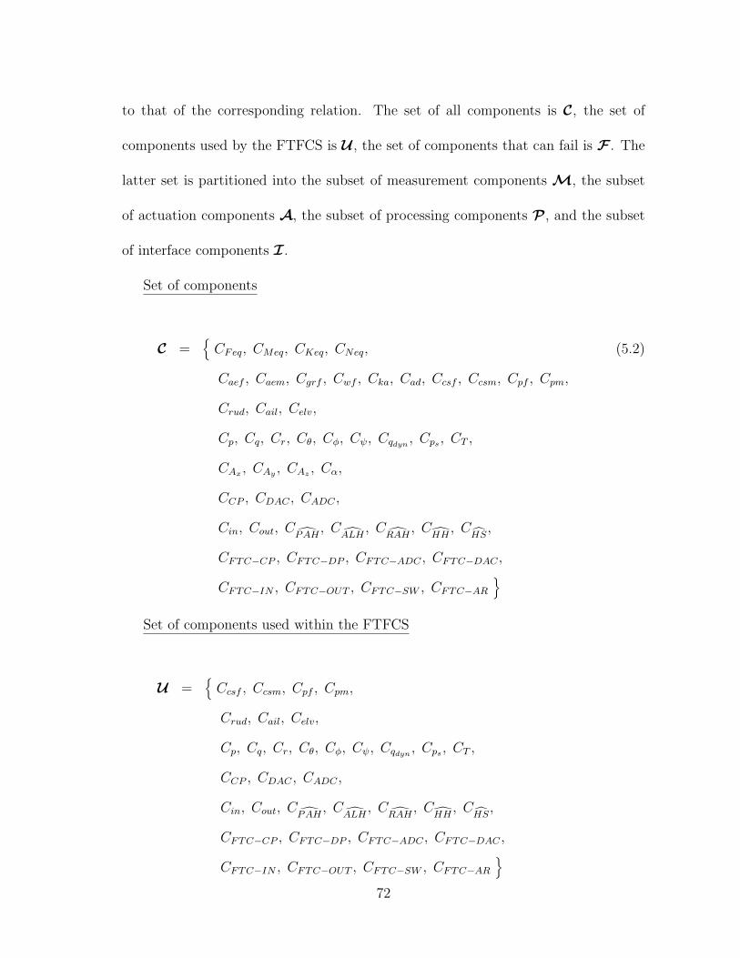
to that of the corresponding relation. The set of all components is C, the set of
components used by the FTFCS is U , the set of components that can fail is F . The
latter set is partitioned into the subset of measurement components M, the subset
of actuation components A, the subset of processing components P , and the subset
of interface components I .
Set of components
C ={
CFeq, CMeq, CKeq, CNeq, (5.2)
Caef , Caem, Cgrf , Cwf , Cka, Cad, Ccsf , Ccsm, Cpf , Cpm,
Crud, Cail, Celv,
Cp, Cq, Cr, Cθ, Cφ, Cψ, Cqdyn, Cps , CT ,
CAx , CAy , CAz , Cα,
CCP , CDAC , CADC ,
Cin, Cout, CPAH
, CALH
, CRAH
, CHH
, CHS
,
CFTC−CP , CFTC−DP , CFTC−ADC , CFTC−DAC ,
CFTC−IN , CFTC−OUT , CFTC−SW , CFTC−AR
}Set of components used within the FTFCS
U ={
Ccsf , Ccsm, Cpf , Cpm,
Crud, Cail, Celv,
Cp, Cq, Cr, Cθ, Cφ, Cψ, Cqdyn, Cps , CT ,
CCP , CDAC , CADC ,
Cin, Cout, CPAH
, CALH
, CRAH
, CHH
, CHS
,
CFTC−CP , CFTC−DP , CFTC−ADC , CFTC−DAC ,
CFTC−IN , CFTC−OUT , CFTC−SW , CFTC−AR
}72

Set of fallible components
F ={
Ccsf , Ccsm, Cpf , Cpm, (5.3)
Crud, Cail, Celv,
Cp, Cq, Cr, Cθ, Cφ, Cψ, Cqdyn, Cps , CT ,
CAx , CAy , CAz , Cα,
CCP , CDAC , CADC ,
Cin, Cout, CPAH
, CALH
, CRAH
, CHH
, CHS
,
CFTC−CP , CFTC−DP , CFTC−ADC , CFTC−DAC ,
CFTC−IN , CFTC−OUT , CFTC−SW , CFTC−AR
}Set of Measurement components
M ={
Cp, Cq, Cr, Cθ, Cφ, Cψ, Cqdyn, Cps , CT , (5.4)
CAx , CAy , CAz , Cα
}Set of Actuation components
A ={
Ccsf , Ccsm, Cpf , Cpm, Crud, Cail, Celv
}(5.5)
Set of Processing components
P ={
CALH
, CRAH
, CHH
, CHS
, (5.6)
CFTC−IN , CFTC−OUT , CFTC−SW , CFTC−AR
}Set of Interface components
I ={
CCP , CDAC , CADC , (5.7)
CFTC−CP , CFTC−DP , CFTC−ADC , CFTC−DAC
}73

5.2.2 Formal specification of fault hypotheses
A fault hypothesis consists in the assignment to each fallible component of a mode
of operation that is either described by the component specification or by one of
the component fault-modes. For each component Cc, Rc denotes the relation that
specifies its requirement, Fc denotes the set of its fault-mode relations, and Rc,n
denotes the relation that specifies its fault-mode number n. Rc(H) denotes the
behaviour of component Cc under fault hypothesis H and the term H∗ denotes any
of the fault hypotheses. For the sake of space the definition of fault hypothesis HM0
is explicit, while the other fault hypothesis definitions refer to this one.
Fault hypothesis HM0
Measurement components used by the FTFCS
∀m(Cm ∈ M ⋂ U ⇒ Rm(HM0) = Rm
)(5.8)
Processing components used by the FTFCS
∀ c(Cc ∈ P ⋂ U ⇒ Rc(H∗) = Rc
)(5.9)
Interface components used by the FTFCS
∀ c(Cc ∈ I ⋂ U ⇒ Rc(H∗) = Rc
)(5.10)
Actuation components used by the FTFCS
∃ a ∃ f ∃ b ∃ g(Ca ∈ A ⋂ U ∧ Ra,f ∈ Fa ∧ (5.11)
Cb ∈ A ⋂ U ∧ Rb,g ∈ Fb ⇒( Ra(H∗) = Ra,f ∨ Ra(H∗) = Ra ) ∧( Rb(H∗) = Rb,g ∨ Rb(H∗) = Rb ) ∧∀ c
(c 6= a ∧ c 6= b ∧ Cc ∈ A ⋂ U ⇒ Rc(H∗) = Rc
))74

Components not used by the FTFCS
∀ c(Cc ∈ F \ U ⇒ Rc(H∗) = Rc ∨ (5.12)
∃ f(
Rc,f ∈ Fc ⇒ Rc(H∗) = Rc,f
))
Fault hypothesis HM1,m
Measurement components used by the FTFCS
∃ f(Cm ∈ M ⋂ U ∧ Rm,f ∈ Fm ⇒ (5.13)
Rm(HM1) = Rm,f
)∧
∀n(
n 6= m ∧ Cn ∈ M ⋂ U ⇒ Rn(HM1) = Rn
)
All other fallible components: same as for fault hypothesis HM0
Fault hypothesis HM2
Measurement components used by the FTFCS
∃m ∃ f ∃n ∃ g(Cm ∈ M ⋂ U ∧ Rm,f ∈ Fm ∧ (5.14)
Cn ∈ M ⋂ U ∧ Rn,g ∈ Fn ⇒Rm(HM2) = Rm,f ∧ Rn(HM2) = Rn,g ∧∀ c
(c 6= m ∧ c 6= n ∧ Cc ∈ M ⋂ U ⇒
Rc(HM2) = Rc ∨∃h
(Rc,h ∈ Fc ⇒ Rc(HM2) = Rc,h
)))
All other fallible components: same as for fault hypothesis HM0
5.2.3 Relational specification of the FTC-AR requirements
The relations of this section specify the fault tolerance requirements of section 5.1.3.
RENV (H) describes the environment of the FTC-AR block under fault hypothesis
75

H; this relation capture the actual correlation between software variables representing
airplane state and actuator inputs. RFTC−OFF specifies the requirements for FTC
disengaged, RFTC−DI specifies the detection and identification requirements under
all fault hypotheses, and RFTC−R specifies the recovery requirements.
RENV (H) = (5.15){(Uc, X
)∣∣∣ ∃U ′w ∃U ′
pm ∃U ′c ∃ U ′
c ∃U ′pa ∃X ′
((Uc, U ′
c
)∈ Rout(H) ◦ RDAC(H) ∧(
( U ′c,X ′ ), U ′
c
)∈ Rail(H) t Relv(H) t Rrud(H) ∧(
( U ′c,U ′
pm,U ′w,X ′ ), X ′
)∈
RKeq t RNeq t Rad t Rka t(Raef t Rgrf t Rcsf(H) t Rpf(H) t Rwf
)◦RFeq t(
Raem t Rcsm(H) t Rpm(H))◦RMeq ∧(
( U ′pa,X ′ ), X
)∈
(Rp(H) t Rq(H) t Rr(H) t
Rψ(H) t Rθ(H) t Rφ(H) t Rps(H) t Rqdyn(H) t RT (H) t
RAx(H) t RAy (H) t RAz (H) t Rα(H) t RCP (H))◦
RADC(H) ◦ Rin(H))}
RFTC−OFF = (5.16){(Uf , Yf
)∣∣∣∀ k1 ∀ k2
(0 ≤ k1 < k2 < ∞ ⇒
∀ k(
k1 < k < k2 ∧ SW FTC(k) = OFF ⇒
∀m(Cm ∈ M ⋂ U ⇒ Wm(k) = OFF
)∧ Wdis(k) = OFF
))}
76
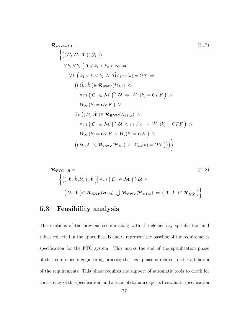
RFTC−DI = (5.17){(( Uf , Uc, X )( Yf )
)∣∣∣∀ k1 ∀ k2
(0 ≤ k1 < k2 < ∞ ⇒
∀ k(
k1 < k < k2 ∧ SW FTC(k) = ON ⇒(( Uc, X )∈ RENV (HM0) ∧∀m
(Cm ∈ M ⋂ U ⇒ Wm(k) = OFF
)∧
Wdis(k) = OFF)
∨∃ c
(( Uc, X )∈ RENV (HM1,c) ∧
∀m(Cm ∈ M ⋂ U ∧ m 6= c ⇒ Wm(k) = OFF
)∧
Wdis(k) = OFF ∧ Wc(k) = ON)
∨(( Uc, X )∈ RENV (HM2) ∧ Wdis(k) = ON
)))}
RFTC−R = (5.18){(( X , X , Uc ), X
)∣∣∣ ∀m(Cm ∈ M ⋂ U ∧
(Uc, X
)∈ RENV (HM0)
⋃ RENV (HM1,m) ⇒(X , X
)∈ RXX
)}
5.3 Feasibility analysis
The relations of the previous section along with the elementary specification and
tables collected in the appendices B and C represent the baseline of the requirements
specification for the FTC system. This marks the end of the specification phase
of the requirements engineering process; the next phase is related to the validation
of the requirements. This phase requires the support of automatic tools to check for
consistency of the specification, and a team of domain experts to evaluate specification
77

completeness and correctness. This is beyond the scope of this research; however,
the feasibility aspect of the validation phase is discussed in some detail. Feasibility
of the fault tolerance requirements is related to detectability of a fault condition,
identifiability of the faulty component, and recoverability of the function provided
by the faulty component. The focus is on detectability and identifiability. Before
analyzing these two items on the basis of the formal specification their interpretation
in the technical literature is illustrated.
5.3.1 Traditional interpretation of detectability and identifi-ability
Fault detectability and identifialbility (or isolability) are relatively new concepts in
the field of fault diagnosis. Only a few papers in the technical literature focus on
these concepts, and present slightly different interpretations. Frank at al. [24] define
a system to be unknown-input fault detectable if for ”almost all faults, an arbitrary
small time interval allows a unique decision for the fault only on considering the
known input and the available output data in this time interval”. According to this
definition fault detectability is a system property that holds for almost all faults.
However, in a system there can be both detectable and undetectable faults at the
same time; an example is provided in [29]. Hence, the above definition leads to too
restrictive detectability conditions. In [32] Horak states that a fault is detectable
if its effects on system outputs overtake the effects of model uncertainties. Using
an optimization procedure based on the Maximum Principle, the maximum possible
deviation between nominal output values and actual output values (reachable mea-
78
surements interval) is derived at each time step. A fault is declared detectable if it
causes the system output to assume values outside the reachable measurement inter-
val. This definition of fault detectability highlights the concept of detection feasibility
in spite of disturbances; however, it differentiates detectable from undetectable faults
in terms of fault effects in time domain only. Faults that add to system output a
low-amplitude, high-frequency component could be detected by analyzing the fre-
quency content of the measurements. Nevertheless, they are undetectable, according
to the definition in [32], if fault effects fall within the reachable measurement interval.
In other definitions fault detectability is either intended as detection capability of a
specific fault detection system [13], or as the best detection capability achievable by
adopting a particular residual generation approach ([23] and [43]). In [11] (sections
2.6 and 2.7) fault detectability and isolability are defined in terms of the fault trans-
fer matrix obtained from the adopted residual generator: a fault is detectable if the
transfer function between the fault input and the residual vector is non-zero; a fault
is identifiable if the residual vector allows distinguishing it from the other faults.
None of the above interpretations provide a definition that is independent of the
specific residual generator adopted and that captures all relevant elements of the de-
tectability and isolability problems. An attempt to provide a definition of detectabil-
ity as a system property (i.e. independent of the adopted residual generator) and
to point out the elements that play a role in the detectability problem can be found
in [29]. In this article fault detectability is defined as follows: ”A fault on a compo-
nent of the system is said to be detectable if knowledge of system inputs and outputs
79
over a finite time interval following the occurrence of the fault allows the detection in
spite of disturbances”. Fault dynamics, disturbance action, and system dynamics are
pointed out as the only elements that play a role in assessing fault detectability. A
detectability analytical criterion is derived from the above definition and formulated
in the frequency domain.
5.3.2 Formal definition of detectability and identifiability
The definition of detectability and identifiability can be formulated on the basis of
the fault detection and identification requirements specified in section 5.1.3:
Detectability condition
- the correlation between Uc and X allows distinguishing between conditions cap-
tured by fault hypothesis HM0 and conditions captured by any of the fault
hypotheses HM1,m and
- the correlation between Uc and X allows distinguishing between conditions cap-
tured by fault hypothesis HM0 and conditions captured by fault hypothesis HM2
and
- the correlation between Uc and X allows distinguishing between conditions cap-
tured by any of the fault hypotheses HM1,m and conditions captured by fault
hypothesis HM2;
Identifiability
- The correlation between Uc and X allows distinguishing between conditions
captured by any couple of fault hypotheses HM1,m and HM1,n
The above definition can be formalized as follows:
80

∀m(Cm ∈ M ⋂ U ⇒ (5.19)
RENV (HM0)⋂ RENV (HM1,m) = Ø ∧
RENV (HM2)⋂ RENV (HM1,m) = Ø
)∧
RENV (HM2)⋂ RENV (HM0) = Ø
∀m ∀n(
m 6= n ∧ Cm ∈ M ⋂ U ∧ Cn ∈ M ⋂ U ⇒ (5.20)
RENV (HM1,m)⋂ RENV (HM1,n) = Ø
)
The interpretation of the detectability condition 5.19 is straightforward when an-
alyzed along with the detection requirement 5.17; it simply states that under no
conditions two out of the three OR operands in the relation RFTC−DI are simulta-
neously true. It is worth noting that all elements pointed out in [29] are present in
the above detectability definition: the fault dynamics is captured by the fault mode
specified within the fault hypothesis, while the system dynamics and the disturbances
are modeled within RENV ().
81

Chapter 6
Conclusions
The outcome of this research work is the formal specification of the requirements
for the FTC system. This system interfaces with the AFCS to provide fault toler-
ance capability with respect to sensor failures. The developed specification represents
the baseline specification for the FTC system, the starting point for the refinement
iteration that takes place within the system life-cycle. The FTC specification was
formulated on top of the AFCS performance specification and of the DHC-2 detail
specification. The fault tolerance requirements were extracted from the active military
specification MIL-F-9490D and translated in the context of analytical redundancy af-
ter a detailed analysis of the implications of adopting this redundancy approach. The
long process of analysis, modeling, and specification of the FTC requirements resulted
in a clear definition of the fault tolerance problem in the framework of analytical re-
dundancy. Furthermore, it brought up to light important issues in all fields involved
in the process, namely FTFCS specification, analytical redundancy, and requirements
engineering. These issues and the lessons learned are summarized below.
The re-engineering process of the active FCS specification uncovered the ambi-
guity and incompleteness of the FCS performance and fault tolerance requirements.
82
These potentially dangerous characteristics of the FCS specification might not repre-
sent a treat since in practice the objectives of FCS certification go way beyond the
fulfillment of the written requirements; however, they do highlight the immaturity
of the specification. Mature and formally specified requirements would result in a
more effective design and a more efficient certification process eventually supported
by automated tools.
A first observation about the analytical redundancy approach is that it can only
be used to provide fault tolerance with respect to failure of components that are
functionally redundant within the system. This implies that some degree of physical
redundancy is required within the FTFCS.
Two important characteristics of analytical redundancy based solutions originate
from these systems being subordinated to the operation of a considerable number of
components of their environment. This dependence has an impact on the modularity
and certifiability of the FTC system. If different FTC modules are to be adopted for
different classes of components a priority ordering must be specified. This ordering
determines a stratified architecture of the FTC system where for each FTC module,
faults of components monitored at the lower layers are transparent, while faults of
components monitored at the upper layers are not. Despite the modularity of the
FTC architecture fault tolerance requirements for each FTC module must be total
with respect to operation of all fallible components. The priority ordering and the
totality characteristic of fault tolerance requirements diminish the typical advantages
of the modular approach.
83
The FTC intrinsic dependence on the dynamics of the aircraft also raises a signif-
icant issue in the certification of such systems: they potentially require a certification
process comparable to that adopted in the certification of AFCS’s, with all related
consequences in terms of costs, time, and employed resources. Furthermore, the fault
modes of the aircraft and FTFCS components form the basis of the certification. This
implies that the FTC must be certified against each combination of faulty compo-
nents and fault-modes as captured by the fault hypotheses. The fault modes of all
components whose failures are not transparent to the FTC module come to play a
crucial role in the feasibility of the solution.
The above observations point out some significant implications of adopting the
analytical redundancy approach as a basis for fault tolerance. The core message of
these observations is that the FTC fault tolerance requirements and related certifica-
tion procedures are considerably more demanding than those typically adopted in the
literature. The more stringent requirements should not discourage the FTC designer,
rather they should be regarded as the basis for a more rationale and effective design.
Functional redundancy is a form of redundancy, it provides – to some degree – the
means to achieve fault tolerance. The question is not whether analytical redundancy
can be used, but how to integrate it with physical redundancy to effectively achieve
fault tolerance. Adopting analytical redundancy to reduce the level of physical re-
dundancy in multistring architecture from triple or quadruple to dual would bring
considerable benefits already.
The observations related to requirements engineering converge upon the specifi-
84

cation methodology and the suitability of relational algebra as formal specification
language. A number of issues related to the hierarchical decomposition of the specifi-
cation, to the modeling of the specification, and to the dependencies among variables
that are not part of the system input/output interface caused non-trivial problems.
The lack of a mature methodology for developing the specification of a fairly complex
system as the one under analysis in this research work considerably slowed down the
specification process. Another important issue related to the specification process
is the need of automatic tools to facilitate development and documentation. The
complexity of the specification, the intrinsic interdependence among its parts, and
the continuous need of modifications require a well engineered development environ-
ment. Without automatic development and management tools the use of a formal
specification does not deliver all the benefits it could.
Among the most desirable characteristics of a formal specification language the
author lists monotonicity. Monotonicity is a fundamental feature, it allows modifying
and updating the specification over time, thus providing continuity and consistency
during the development of the specification. If it is true – and it is – that the formaliza-
tion process of requirements leads to a better understanding of the problem to address,
then the requirements are continuously updated during this process. This explains
why monotonicity is so important. The author’s experience with non-monotonic spec-
ification languages ended up with useless specifications. Monotonicity of relational
algebra was one of the features that pointed toward its choice, to damage of other
languages that come with support tools. Another advantage of relational algebra
85

is that predicate logic specifications are readable and do not require any unnatural
translation into a rigid specification model.
The development of a formal specification requires a considerable amount of re-
sources. On the other hand, the efforts employed at producing a formal specification
pay off with a remarkable understanding of the problem under analysis and an un-
ambiguous and upgradable formulation of the requirements. Formal specification is
advisable whenever the system under development raises safety issues.
86

Bibliography
[1] Background information and user guide for MIL-F-9490D. Technical reportAFFDL-TR-74-116, USAF, 1975.
[2] Flight control systems - design, installation and test of piloted aircraft, generalspecification for. Military specification MIL-F-9490D, USAF, 1975.
[3] Appendix to background information and user guide for MIL-F-9490D. Technicalreport AFFDL-TR-74-116 sup1, USAF, 1980.
[4] Flying qualities for piloted airplanes. Technical Report MIL-F-8785C, USAF,1980.
[5] Background information and user guide for MIL-F-8785C. Technical reportAFWAL-TR-81-3109, USAF, 1982.
[6] IEEE guide for developing system requirements specifications. Standard IEEEStd 1233, IEEE, 1998.
[7] B. D. Appleby, J. R. Dowdle, and W. Vander Velde. Robust estimator designusing µ synthesis. Proc. of the 30th conference on Decision and Control, pages640–644, 1991.
[8] M. Basseville. Detecting changes in signals and systems - a survey. Automatica,24:309–326, 1988.
[9] B. W. Boehm. Verifyng and validating software requirements and design speci-fications. IEEE Software, 1:75–88, 1984.
[10] F. W. Burcham, T. A. Maine, and C. Gordon. Development and flight test ofan emergency flight control system using only engine thrust on an F-15 aircraft.Technical Report 94-02, NASA Dryden Flight Reserach Center, 1994.
[11] J. Chen and R.J. Patton. Robust Model-Based Fault Diagnosis for DynamicSystems. Kluwer Academic Publishers, 1999.
[12] J. Chen and H. Y. Zhang. Parity vector approach for detecting failures in dy-namic systems. Int. Journal Sys. Sci., pages 765–770, 1990.
87

[13] Jie Chen and R.J. Patton. A re-examination of fault detectability and isolabilityin linear dynamic systems. Fault Detection, Supervision and Safety for TechnicalProcesses, pages 567–73, 1994.
[14] E. Y. Chow and A. S. Willsky. Issues in the development of a general algorithmfor reliable failure detection. Proc. of the 19th Conf. on Decision and Control,1980.
[15] E. Y. Chow and A. S. Willsky. Analytical redundancy and the design of robustdetection systems. IEEE Trans. on Automatic Control, 29:603–614, 1984.
[16] R. N. Clark. The dedicated observer approah to instrument failure detection.Proc. of the 18th IEEE Conf. on Decision and Control, pages 237–241, 1979.
[17] J. C. Deckert, M. N. Desai, J. J. Deyst, and A. S. Willsky. F-8 DFBW sensor fail-ure identification using analytical redundancy. IEEE Transactions on AutomaticControl, 22:795–803, 1977.
[18] X. Ding, L. Guo, and P. M. Frank. A frequency domain approach to faultdetection of uncertain systems. Proc. of the 32nd IEEE Conference on Decisionand Control, pages 1722–1727, 1993.
[19] M. Dorfman. Requirements engineering. Software Requirements Engineering,pages 7–22, 1997.
[20] Brooks F. No silver bullet: Essence and accidents of software engineering. Com-puter, April 1987.
[21] C. Favre. Fly-by-wire for commercial aircraft: The airbus experience. Interna-tional Journal of Control, 59:139–157, 1994.
[22] P. M. Frank. Fault diagnosis in dynamic system via state estimation - a survey.in Tzafestas, Singh, and Shmidt (Eds.), System Fault Diagnostics, Reliabilityand Related Knowledge-based Approaches, D. Reidel Press, Dordrecht, pp.35-98,1987.
[23] P. M. Frank and J. Wunnenberg. Robust fault diagnosis using unknown inputschemes. in R. J. Patton, P. M. Frank, and R. N. Clark (Eds.), ”Fault Diagnosisin Dynamic Systems: Theory and Application”, Prentice Hall, chapter 3, pp.47-98, 1989.
[24] P.M. Frank and B. Koppen. Review of optimal solutions to the robustness prob-lem in observer-based fault detection. Journal of Systems and Control Engineer-ing, 207(12):105–12, 1993.
[25] J. Gertler. Fault detection and isolation using parity relations. Control Eng.Practice, 5:653–661, 1997.
88

[26] J. Gertler and M. Costin. Model-based diagnosis of automotive engines-casestudy on a physical vehicle. IFAC Symposium on Fault Detection, Supervisionand Safety for Technical Processes - SAFEPROCESS ’94, 2:421–430, 1994.
[27] J. Gertler and G. DiPierro. On the relationship between parity relations andparameter estimation. Proc. of the IFAC Sympo. on Fault Detection, Supervisionand Safety for Technical Processes: SAFEPROCESS’97, pages 453–458, 1997.
[28] J. Gertler, Q. Luo, K. Anderson, and X. W. Fang. Diagnosis of plant failuresusing orthogonal parity equations. Proc. of the 11th IFAC World Congress, 1990.
[29] D. Del Gobbo and M. Napolitano. Issues in fault detectability for dyanmicsystems. American Control Conference, 2000.
[30] D. M. Himmelblau. Fault detection in heat exchangers. Proceedings of the 1992American Control Conference, 2:2369–2372, 1992.
[31] D. E. Hoak, D. E. Ellison, and et al. USAF Stability and Control DAT-COM. Flight Control Division, Air Force Flight Dynamics Laboratory; Wright-Patterson Air Force Base, Ohio., 1968.
[32] D.T. Horak. Failure detection in dynamic systems with modeling errors. Journalof Guidance, Control, and Dynamics, 11(6):508–16, 1988.
[33] R. Isermann. Process fault detection based on modelling and estimation methods:A survey. Automatica, 20:387–404, 1984.
[34] R. Isermann. Experiences with process fault detection via parameter estimation.in Tzafestas, Singh, and Shmidt (Eds.), System Fault Diagnostics, Reliabilityand Related Knowledge-based Approaches, D. Reidel Press, Dordrecht, pp. 3-33,1987.
[35] R. O. Lewis. Independent Verification and Validation: A Life Cycle EngineeringProcess for Quality Software. John Wiley & Sons, 1992.
[36] Jackson M. The meaning of requirements. Annals of Software Engineering,3:5–21, 1997.
[37] Rauw M. FDC 1.2 - A Simulink toolbox for flight dynamics and control analysis- user manual. http://www.mathworks.com/, 1998.
[38] Rauw M.O. A Simulink environment for flight dynamics and control analysis -application to the DHC-2 ’beaver’. Graduate’s thesis. Delft Univ. of Thechnology,the Netherlands, 1993.
[39] M. R. Napolitano, V. Casdorph, C. Neppach, S. Naylor, M. Innocenti, and G. Sil-vestri. Online learning neural architectures and cross-correlation analysis foractuator failure detection and identification. International Journal of Control,63:433–455, 1996.
89
[40] M. R. Napolitano, C. I. Chen, and S. Naylor. Aircraft failure detection and iden-tification using neural networks. Journal of Guidance, Control, and Dynamics,16:999–1009, 1993.
[41] M. R. Napolitano, D. A. Windon, J. L. Casanova, M. Innocenti, and G. Silvestri.Kalman filters and neural-network schemes for sensor validation in flight controlsystems. IEEE Transactions on Control Systems Technology, 6:596–611, 1998.
[42] B. A. Nuseibeh and S. M. Easterbrook. Requirements engineering: A roadmap.Proceedings, 22nd International Conference on Software Engineering (ICSE’00),pages 35–46, June 4-11 2000.
[43] M. Nyberg and L. Nielsen. Parity functions as universal residual generatorsand tool for fault detectability analysis. 36th IEEE Conference on Decision andControl, 5:4483–9, 1997.
[44] S. Osder. Practical view of redundancy management-application and theory.Journal of Guidance, Control, and Dynamics, 22:12–21, 1999.
[45] J. H. Park, Y. Halevi, and G. Rizzoni. A new interpretation of the fault-detectionfilter. 2: Theoptimal detection filter. Int. Journal of Control, 60:1339–1351, 1994.
[46] J. H. Park and G. Rizzoni. A new interpretation of the fault-detection filter. 1:Closed-form algorithm. Int. Journal of Control, 60:767–787, 1994.
[47] R. J. Patton. Robust model-based fault diagnosis: The state of the art. IFACSymposium on Fault Detection, Supervision and Safety for Technical Processes -SAFEPROCESS ’94, 1:1–24, 1994.
[48] R. J. Patton and J. Chen. A re-examination of the relationship between parityspace and observer-based approaches in fault diagnosis. European Journal ofDiagnosis and Safety in Automation, 1:183–200, 1991.
[49] R. J. Patton and J. Chen. Robust fault detection of jet engine sensor systemsusing eigenstructure assignment. Journal of Guidance, Control and Dynamics,15:1491–1497, 1992.
[50] R. J. Patton, J. Chen, and C. J. Lopez-Toribio. Fuzzy observers for non-lineardynamic systems fault diagnosis. Proceedings of the 37th IEEE Conference onDecision and Control, 1:84–89, 1998.
[51] R.J. Patton, P. M. Frank, and R. N. Clark (Eds.). Issues of Fault Diagnosis forDynamic Systems. Springer Verlag, 2000.
[52] Patton R.J., Frank P., and Clark R. Fault Diagnosis in Dynamic Systems, Theoryand Applications. Prentice Hall, 1989.
90
[53] Tjee R.T.H. and Mulder J.A. Stability and control derivatives of the De Hav-illand DHC-2 ’beaver’ aircraft. Report LR-556, Delft Univ. of Technology, TheNetherlands, 1988.
[54] M. A. Sadrnia, J. Chen, and R. J. Patton. Robust fault detection observerdesign using H∞/µ techniques for uncertain falight control systems. Proc. of the2ndIFAC Symposium on Robust Control Design: RECOND97, pages 531–536,1997.
[55] G. Schmidt and T. Strohlein. Relations and Graphs. Springer Verlag, 1993.
[56] K.J. Szalai, R.R. Larson, and R.D. Glover. Flight experience with flight controlredundancy management. In AGARD Lecture Series No.109. Fault ToleranceDesign and Redundancy Management Techniques, AGARD Lecture Series, pages8/1–27, AGARD, Neuilly-sur-Seine, France, October 1980. AGARD.
[57] A. T. Vemuri and M. M. Polycarpou. Neural-network-based robust fault diag-nosis in robotic systems. IEEE Transactions on Neural Networks, 8:1410–1420,1997.
[58] Alagar V.S. and Periyasamy K. Specification of Software Systems. SpringerVerlag, 1998.
[59] J. L. Weiss and J. Y. Hsu. Design and evaluation of a failure detection andisolation algorithm for restructurable control systems. Technical Report NASA-CR-178213, 1985.
[60] A. S. Willsky. A survey of design methods for failure detection in dynamicsystems. Automatica, 12:601–611, 1976.
[61] A. S. Willsky, J. J. Deyst, and B. S. Crawford. Adaptive filtering and self-test methods for failured detection and compensation. Proc. of the 1974 JointAmerican Control Conf., pages 637–645, 1974.
[62] Y.C. Yeh. Triple-triple redundant 777 primary flight computer. IEEE AerospaceApplications Conference, February 1996.
91

Appendix A
Predicate Logic and RelationalAlgebra
This appendix provides a formal definition of syntax and semantics of predicate logic
and relational algebra. Predicate logic is the formal language adopted in relational
specifications. Relational algebra is the mathematical framework that allows operat-
ing with relational specifications. The content of this appendix serves as support to
chapters 4 and 5, and to appendix B. The presented information is largely based on
references [55] and [58].
A.1 Logic
Logic can be used as a formal specification language. Examples of logic include
propositional logic and first-order predicate logic. The information presented in this
section provides a brief description of the language aspects of logic.
A.1.1 Propositional logic
A proposition is a statement that is either True (T ) or False (F ). Propositional logic
consists of sentences constructed from atomic formulas and the logical connectives
92

Table A.1: Syntax of propositional logic
terminals = {P, Q, R, . . . , ¬ , ∧ , ∨ , ⇒ , ⇔ , (, ); }nonterminals = {atomic formula, sentence};atomic formula = P | Q | R | . . . ;sentence = atomic formula | (, sentence, ) | ¬ , sentence |
sentence, ∧ , sentence |sentence, ∨ , sentence |sentence, ⇒ , sentence |sentence, ⇔ , sentence;
∧ (and), ∨ (or), ¬ (not), ⇒ (if ... then), ⇔ (if and only if ). Atomic formulas
are the simplest form of propositions. Examples of atomic formulas are:
3 > 2a > 5a > b
Examples of sentences are:
3 > 2 ∧ 2 > 1a > 2 ⇒ b > 1a > b ∧ b > 2 ⇒ c > 2
Table A.1 defines the syntax of the language by means of the Backus Naur for-
malism, while table A.2 defines its semantics. The logic operators are subject to the
following precedence ordering: ¬ , ∧ , ∨ , ⇒ , ⇔ ; ¬ being the operator with
highest precedence. The semantics of a sentence is obtained by assigning truth values
(T or F ) to atomic formulas and evaluating the sentences according to the semantics
of the language.
A.1.2 Predicate logic
Table A.3 defines the syntax of predicate logic. Constants and connectives are in-
terpreted as in propositional logic. Predicates are functions that evaluate either true
93
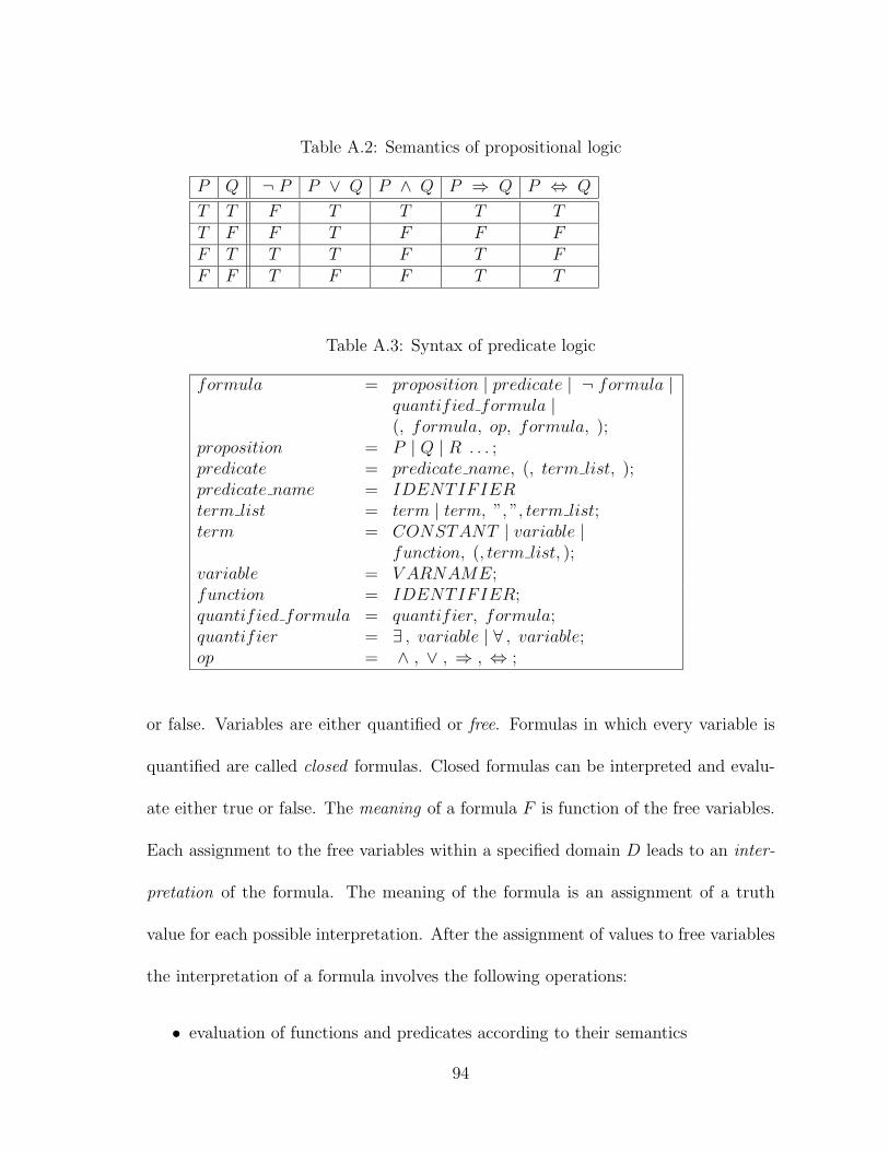
Table A.2: Semantics of propositional logic
P Q ¬ P P ∨ Q P ∧ Q P ⇒ Q P ⇔ Q
T T F T T T TT F F T F F FF T T T F T FF F T F F T T
Table A.3: Syntax of predicate logic
formula = proposition | predicate | ¬ formula |quantified formula |(, formula, op, formula, );
proposition = P | Q | R . . . ;predicate = predicate name, (, term list, );predicate name = IDENTIFIERterm list = term | term, ”, ”, term list;term = CONSTANT | variable |
function, (, term list, );variable = V ARNAME;function = IDENTIFIER;quantified formula = quantifier, formula;quantifier = ∃ , variable | ∀ , variable;op = ∧ , ∨ , ⇒ , ⇔ ;
or false. Variables are either quantified or free. Formulas in which every variable is
quantified are called closed formulas. Closed formulas can be interpreted and evalu-
ate either true or false. The meaning of a formula F is function of the free variables.
Each assignment to the free variables within a specified domain D leads to an inter-
pretation of the formula. The meaning of the formula is an assignment of a truth
value for each possible interpretation. After the assignment of values to free variables
the interpretation of a formula involves the following operations:
• evaluation of functions and predicates according to their semantics
94

• evaluation of propositions and non-quantified sub-formulas according to the
semantics of propositional logic
• evaluation of quantified formulas according to the following semantics:
– a quantified formula of the type ∀x F evaluates true if F is true for every
value of x in the domain of interpretation; otherwise it evaluates false
– a quantified formula of the type ∃x F evaluates true if there exists at least
one value of x within the domain of interpretation for which F is true;
otherwise it evaluates false
Each operation is carried out to reduce the arguments of the formula until the truth
value of the formula can be determined.
A.2 Relational algebra and requirements specifi-
cation
Predicate logic provides means to formally specify requirements. Relational algebra
provides the formal framework for reasoning with requirement specifications. The
following section introduces the main concepts of relational algebra, while the last
section illustrates the main concepts of relational specification.
A.2.1 Basics of relational algebra
Given two spaces (or sets) A and B, a relation R over A × B is a subset of A × B
and is specified as follows:
R = {(A,B) | F (A,B)} (A.1)
95

The above expression reads: relation R is the set of couples of elements (A,B) ∈
A × B such that F (A,B) evaluates true. F is a predicate logic formula and is speci-
fied according to syntax and semantics rules presented in section A.1.2. In the follow-
ing each relation is assumed to be over the space A × B unless otherwise specified.
Definitions
Relation domain and range If (A,B) is an element of relation R, then A is called
an antecedent of R and B an image of R. The set of images of A by relation R
is denoted by A • R, and the set of antecedents of element A by relation R is
denoted by R •A. The set of all antecedents of R is the domain of relation R
and is denoted dom(R). The set of all images of R is the range (or codomain)
of relation R and is denoted rng(R).
Universal relation The universal (or total) relation over the set A is defined by
A × A and is denoted LA.
Identity relation The identity relation over the set A is defined by {(A,A′) | A =
A′} and is denoted by IA. Given a set S ⊆ A we define IA(S) = {(A,A′) |
A ∈ S ∧ A = A′}.
Operations on relations
Since relations are sets, they inherit set operators: P(S) (power set), S (comple-
ment), × (cartesian product),⋂
(intersection), \ (difference),⋃
(union), and
the inclusion ordering ⊇ . The precedence ordering of the set operators is the one
adopted in introducing them; the power set operator being the one with highest
96
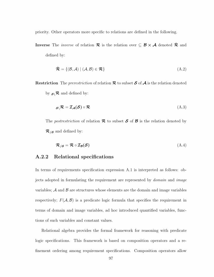
priority. Other operators more specific to relations are defined in the following.
Inverse The inverse of relation R is the relation over ⊆ B × A denoted R and
defined by:
R = {(B,A) | (A,B) ∈ R} (A.2)
Restriction The prerestriction of relation R to subset S of A is the relation denoted
by S\R and defined by:
S\R = IA(S) ◦ R (A.3)
The postrestriction of relation R to subset S of B is the relation denoted by
R/S and defined by:
R/S = R ◦ IB(S) (A.4)
A.2.2 Relational specifications
In terms of requirements specification expression A.1 is interpreted as follows: ob-
jects adopted in formulating the requirement are represented by domain and image
variables; A and B are structures whose elements are the domain and image variables
respectively; F (A,B) is a predicate logic formula that specifies the requirement in
terms of domain and image variables, ad hoc introduced quantified variables, func-
tions of such variables and constant values.
Relational algebra provides the formal framework for reasoning with predicate
logic specifications. This framework is based on composition operators and a re-
finement ordering among requirement specifications. Composition operators allow
97
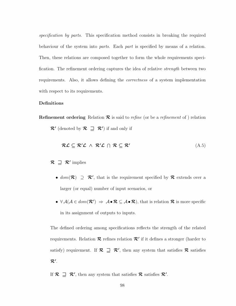
specification by parts. This specification method consists in breaking the required
behaviour of the system into parts. Each part is specified by means of a relation.
Then, these relations are composed together to form the whole requirements speci-
fication. The refinement ordering captures the idea of relative strength between two
requirements. Also, it allows defining the correctness of a system implementation
with respect to its requirements.
Definitions
Refinement ordering Relation R is said to refine (or be a refinement of ) relation
R′ (denoted by R w R′) if and only if
RL ⊆ R′L ∧ R′L ⋂ R ⊆ R′ (A.5)
R w R′ implies
• dom(R) ⊇ R′, that is the requirement specified by R extends over a
larger (or equal) number of input scenarios, or
• ∀A(A ∈ dom(R′) ⇒ A•R ⊆ A•R), that is relation R is more specific
in its assignment of outputs to inputs.
The defined ordering among specifications reflects the strength of the related
requirements. Relation R refines relation R′ if it defines a stronger (harder to
satisfy) requirement. If R w R′, then any system that satisfies R satisfies
R′.
If R w R′, then any system that satisfies R satisfies R′.
98

Correctness A system implementation P is said to be correct with respect to its
specification R if and only if
P w R (A.6)
Product The product of relation R1 ⊆ A × K by relation R2 ⊆ K × B is the
relation over A × B denoted by R1 ◦ R2 (or R1R2) and defined by:
R1 ◦ R2 = {(A,B) | ∃K ((A,K) ∈ R1 ∧ (K,B) ∈ R2)} (A.7)
Join The sum of the requirement information of two relations R1 ⊆ A × B and
R2 ⊆ A × B is called the join of R1 and R2 and is denoted by R1 t R2.
The join of two relations is defined as follows:
R1 t R2 = R1
⋂ R2L⋃ R2
⋂ R1L⋃ R1
⋂ R2 (A.8)
The following implication holds:
R w R1 t R2 ⇔ R w R1 ∧ R w R2 (A.9)
The join exists if and only if R1 and R2 do not contradict each other. The
consistency condition to check whether the join of relations R1 and R2 exists
is the following:
R1L⋂ R2L =( R1
⋂ R2 ) L (A.10)
99

Meet The common requirement information of two relations R1 ⊆ A × B and
R2 ⊆ A × B is called the meet of R1 and R2 and is denoted by R1 u R2.
The meet of two relations is defined as follows:
R1 u R2 = R1L⋂ R2L
⋂( R1
⋃ R2 ) (A.11)
The following implication holds:
R = R1 u R2 ⇒ R1 w R ∧ R2 w R (A.12)
Expansion operation If R is a relation over the space S = A × B, its expansion
over the space S′ = (A, A′) × (B, B′) is defined as follows:
σS′S ◦ R ◦ σS′
S (A.13)
where the operator σS′S is defined by:
σS′S =
{(S,S ′) | A(S) = A(S ′) ∧ B(S) = B(S ′)
}(A.14)
The expansion operation is used to expand the spaces over which the relation
is defined in order to apply the composition operators.
In a relational specification operators from relational algebra, set theory, and
logic may be found in the same expression (see eq. A.5). The precedence between
this class of operators is the following: relational operators are evaluated first, then
set operators, then logic operators. The precedence ordering between operators of
the same class has been defined in section A.1.1 for the logic operators, and in section
100

A.2.1 for the set operators. The precedence ordering among relational operators is
the following: restriction, inverse, complement, product, meet, join; restriction being
the operator with higher priority.
101
Appendix B
Elementary specifications of theAR-FTC environment
This appendix collects the elementary specifications of the AR-FTC environment.
Requirements are specified by means of relations according to the syntax and se-
mantics introduced in appendix A. Elementary specifications are separated into five
different sections. Section B.1 collects relations used in the AFCS performance spec-
ification, section B.2 collects relations used in the DHC-2 detail-specification, section
B.3 collects relations describing fault-modes, section B.4 collects the restriction sets,
and section B.5 collects relations describing the interface blocks of the FTC system
to the AR-FTC module.
102
B.1 Elementary requirements of AFCS performance
specification
3.1.2 AFCS performance requirements ... Unless otherwise specified, theserequirements apply in smooth air and include sensor error. ...
3.1.2.1 Attitude Hold (pitch and roll)
a) Attitudes (θ(), φ() ∈ I) shall be maintained in smooth air (turb() ∈ A) with astatic accuracy of ±0.5 degree in pitch attitude (θacc ∈ C)
b) (with wings level) (phi() ∈ D; φacc ∈ C)
c) and ±1.0 degree in roll attitude (φacc ∈ C) with respect to the reference(θr(), φr() ∈ D; constRef() ∈ A).
d) RMS (RMS() ∈ A) attitude deviations shall not exceed 5 degrees in pitch(θRMS ∈ C)
e) or 10 degrees in roll attitude (φRMS ∈ C) in turbulence (turb() ∈ A) at theintensities specified in 3.1.3.7 (uwt(), vwt(), wwt(), uwg(), vwg(), wwg() ∈ D).
f) Accuracy requirements shall be achieved and maintained within 5 seconds (Tθ, Tφ ∈C) of mode engagement (SWPAH(), SWRAH() ∈ D; engaged() ∈ A)
g) for a 5 degree attitude disturbance (∆θ∗, ∆φ∗ ∈ C).
Intermediate specification (PAH)
FOR EVERY couple of time instants t1, t2
IF
- [t1, t2] is a time interval within [0,∞) AND
f) the length of the time interval [t1, t2] is larger than Tθ AND
b) the aircraft is wings level throughout the interval [t1, t2] AND
- the PAH control function is engaged at t = t1 and stays engagedthroughout the interval [t1, t2] AND
- the reference pitch is constant throughout the interval [t1, t2] AND
g) the pitch deviation from the reference at engagement is ∆θ∗
THEN
a) IF there is no turbulence within the time interval [t1, t2] THEN thedeviation of the pitch angle from the reference shall not be larger thanθacc at all time instants within the time interval [t1 + Tθ, t2] AND
103
d) IF there is turbulence within the time interval [t1, t2] THEN the RMSvalue of the deviation of the pitch angle from the reference over thetime interval [t1 + Tθ, t2] shall not be larger than θRMS
Relational specification (PAH)
RPAH = (B.1){(( Uw,Up,X ),X ′
)∣∣∣ ∀ t1 ∀ t2(
0 ≤ t1 < t2 < ∞ ∧ t2 > t1 + Tθ ∧
∀ t(
t1 ≤ t ≤ t2 ⇒ |φ(t)| < φacc
)∧
engaged(SWPAH(), t1, t2) ∧constRef(θr(), t1, t2) ∧|θ(t1) − θr(t1)| = ∆θ∗ ⇒(
¬ turb(t1, t2) ⇒ ∀ t(
t1 + Tθ ≤ t ≤ t2 ⇒ |θ(t) − θr(t1)| < θacc
))∧(
turb(t1, t2) ⇒ RMS(θ() − θr(t1), t1 + Tθ, t2) < θRMS
))}
Intermediate specification (RAH)
FOR EVERY couple of time instants t1, t2
IF
- [t1, t2] is a time interval within [0,∞) AND
f) the length of the time interval [t1, t2] is larger than Tθ AND
- the RAH control function is engaged at t = t1 and stays engagedthroughout the interval [t1, t2] AND
- the reference bank is constant throughout the interval [t1, t2] AND
g) the roll deviation from the reference at engagement is ∆φ∗
THEN
c) IF there is no turbulence within the time interval [t1, t2] THEN thedeviation of the bank angle from the reference shall not be larger thanφacc at all time instants within the time interval [t1 + Tφ, t2] AND
e) IF there is turbulence within the time interval [t1, t2] THEN the RMSvalue of the deviation of the bank angle from the reference over thetime interval [t1 + Tφ, t2] shall not be larger than φRMS
104

Relational specification (RAH)
RRAH = (B.2){(( Uw,Up,X ),X ′
)∣∣∣ ∀ t1 ∀ t2(
0 ≤ t1 < t2 < ∞ ∧ t2 > t1 + Tφ ∧engaged(SWRAH(), t1, t2) ∧constRef(φr(), t1, t2) ∧|φ(t1) − φr(t1)| = ∆φ∗ ⇒(
¬ turb(t1, t2) ⇒ ∀ t(
t1 + Tφ ≤ t ≤ t2 ⇒ |φ(t) − φr(t1)| < φacc
))∧(
turb(t1, t2) ⇒ RMS(φ() − φr(t1), t1 + Tφ, t2) < φRMS
))}
3.1.2.2 Heading Hold
a) In smooth air (turb() ∈ A), heading (ψ() ∈ I) shall be maintained within a staticaccuracy of ±0.5 degree (ψacc ∈ C) with respect to the reference (ψr ∈ Q).
b) In turbulence, RMS deviations (RMS() ∈ A; uwt(), vwt(), wwt(), uwg(), vwg(), wwg() ∈D) shall not exceed 5 degrees (ψRMS ∈ C) in heading at the intensities specifiedin 3.1.3.7.
c) When heading hold is engaged (SWHH() ∈ D), the aircraft shall roll (φ() ∈ I)towards wings level.
d) The reference heading shall be that heading that exists when the aircraft passesthrough a roll attitude that is wings level plus or minus a tolerance (φacc ∈ C).
Intermediate specification
FOR EVERY couple of time instants t1, t3
IF
[t1, t3] is a time interval within [0,∞) AND
the HH control function is engaged at t = t1 and stays engagedthroughout the interval [t1, t3]
THEN
there must EXIST a time instant t2 and a reference heading ψr suchthat
c1) t2 is within the interval [t1, t3) AND
c2) the bank angle is approximately zero within the time interval[t2, t3) AND
105
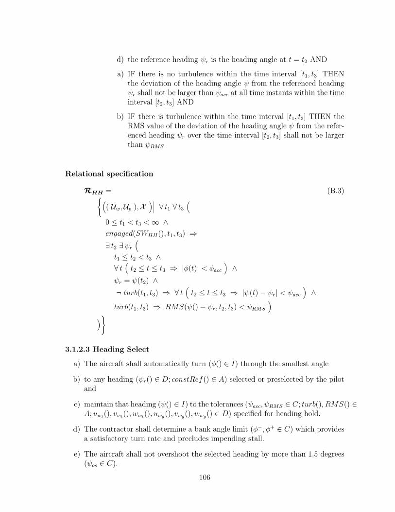
d) the reference heading ψr is the heading angle at t = t2 AND
a) IF there is no turbulence within the time interval [t1, t3] THENthe deviation of the heading angle ψ from the referenced headingψr shall not be larger than ψacc at all time instants within the timeinterval [t2, t3] AND
b) IF there is turbulence within the time interval [t1, t3] THEN theRMS value of the deviation of the heading angle ψ from the refer-enced heading ψr over the time interval [t2, t3] shall not be largerthan ψRMS
Relational specification
RHH = (B.3){(( Uw,Up ),X
)∣∣∣ ∀ t1 ∀ t3(
0 ≤ t1 < t3 < ∞ ∧engaged(SWHH(), t1, t3) ⇒∃ t2 ∃ψr
(t1 ≤ t2 < t3 ∧∀ t
(t2 ≤ t ≤ t3 ⇒ |φ(t)| < φacc
)∧
ψr = ψ(t2) ∧¬ turb(t1, t3) ⇒ ∀ t
(t2 ≤ t ≤ t3 ⇒ |ψ(t) − ψr| < ψacc
)∧
turb(t1, t3) ⇒ RMS(ψ() − ψr, t2, t3) < ψRMS
))}
3.1.2.3 Heading Select
a) The aircraft shall automatically turn (φ() ∈ I) through the smallest angle
b) to any heading (ψr() ∈ D; constRef() ∈ A) selected or preselected by the pilotand
c) maintain that heading (ψ() ∈ I) to the tolerances (ψacc, ψRMS ∈ C; turb(), RMS() ∈A; uwt(), vwt(), wwt(), uwg(), vwg(), wwg() ∈ D) specified for heading hold.
d) The contractor shall determine a bank angle limit (φ−, φ+ ∈ C) which providesa satisfactory turn rate and precludes impending stall.
e) The aircraft shall not overshoot the selected heading by more than 1.5 degrees(ψos ∈ C).
106

f) Entry into and exit from the turn shall be smooth and rapid.
g) The roll rate (p() ∈ I) shall not exceed 10 deg/sec (p+ ∈ C) and
h) roll acceleration shall not exceed 5 deg/sec/sec (p+ ∈ C).
Intermediate specification
FOR EVERY couple of time instants t1, t4
IF
[t1, t4] is a time interval within [0,∞) AND
the HS control function is engaged at t = t1 and stays engaged through-out the interval [t1, t4] AND
the reference heading is constant throughout the interval [t1, t4]
THEN
a) the heading deviation from the reference shall never exceed 180 degreesthroughout the interval [t1, t4] AND
g) The roll rate shall not exceed p+ throughout the interval [t1, t4] AND
h) roll acceleration shall not exceed p+ throughout the interval [t1, t4]AND
d) bank angle shall be in the interval [φ−, φ+] throughout the interval[t1, t4] AND
e) there EXIST a time instant t2 ∈ [t1, t4] when the heading is close tothe reference and it was not close at all time instants within the timeinterval [t1, t2] and it will never get further than ψos at all time instantswithin the time interval [t2, t4]
b), c) there EXIST a time instant t3 ∈ [t2, t4] such that IF there is no tur-bulence within the time interval [t1, t4] THEN the deviation of theheading angle from the referenced heading shall not be larger thanψacc at all time instants within the time interval [t3, t4] AND IF thereis turbulence within the time interval [t1, t4] THEN the RMS value ofthe deviation of the heading angle from the referenced heading overthe time interval [t3, t4] shall not be larger than ψRMS
Relational specification
RHS = (B.4){(( Uw,Up ),X
)∣∣∣ ∀ t1 ∀ t4(
0 ≤ t1 < t4 < ∞ ∧engaged(SWHS(), t1, t4) ∧ constRef(ψr(), t1, t4) ⇒
107

∀ t(
t1 ≤ t ≤ t4 ⇒|ψ(t) − ψr(t1)| ≤ π ∧ φ− < φ(t) < φ+ ∧p(t) < p+ ∧ p(t) < p+
)∧
∃ t2(
t1 ≤ t2 ≤ t4 ∧ |ψ(t2) − ψr(t1)| < ψacc ∧∀ t
(t1 ≤ t ≤ t2 ⇒ |ψ(t) − ψr(t1)| > ψacc
)∧
∀ t(
t2 ≤ t ≤ t4 ⇒ |ψ(t) − ψr(t1)| < ψos
))∃ t3
(t2 ≤ t3 ≤ t4 ∧
¬ turb(t1, t4) ⇒ ∀ t(
t3 ≤ t ≤ t4 ⇒ |ψ(t) − ψr(t1)| < ψacc
)∧
turb(t1, t4) ⇒ RMS(ψ() − ψr(t1)r, t3, t4) < ψRMS
))}
3.1.2.4 Lateral acceleration and sideslip limits ... the following performanceshall be provided whenever any lateral-directional AFCS function is engaged. Lat-eral acceleration refers to apparent (measured, sensed) body axis acceleration at theaircraft center of gravity.
3.1.2.4.1 Coordination in steady banked turns
a) The incremental sideslip angle (β() ∈ I) shall not exceed 2 degrees (∆β+/SBT ∈
C) from the trimmed value (βtr ∈ D),
b) and lateral acceleration (Aycg() ∈ I) shall not exceed 0.03g (A+ycg/SBT ∈ C),
c) while at steady bank angle (φss ∈ Q, φacc ∈ C; φ() ∈ D) up to the maneuverbank angle limit (φ−, φ+ ∈ C) reached during normal maneuvers
d) with the AFCS engaged (SWRAH(), SWHH(), SWHS() ∈ D; whileEngaged() ∈A).
Intermediate specification
FOR EVERY couple of time instants t1, t2
IF
- [t1, t2] is a time interval within [0,∞) AND
d) either RAH, HH, or HS control function is in engaged status through-out the interval [t1, t2] AND
c) the airplane is in a steady bank turn throughout the interval [t1, t2]and the steady bank angle is within allowed limits AND
108

- there is no turbulence throughout the interval [t1, t2]
THEN
a) the sideslip angle deviation from trim value shall not exceed ∆β+/SBT
throughout the interval [t1, t2] AND
b) The lateral acceleration shall not exceed A+ycg/SBT throughout the in-
terval [t1, t2]
Relational specification
RSBT = (B.5){(( Uw,Up,X , Ctr ),X ′
)∣∣∣ ∀ t1 ∀ t2(
0 ≤ t1 < t2 < ∞ ∧(whileEngaged(SWRAH(), t1, t2) ∨
whileEngaged(SWHH(), t1, t2) ∨whileEngaged(SWHS(), t1, t2)
)∧
∃φss
(∀ t
(t1 ≤ t ≤ t2 ⇒ |φ(t) − φss| < φacc
)∧ |φss| > φacc
)∧
¬ turb(t1, t2) ⇒∀ t
(t1 ≤ t ≤ t2 ⇒ |β(t) − βtr| < ∆β+
/SBT ∧ |Aycg(t)| < A+ycg/SBT
))}
3.1.2.4.3 Coordination in straight and level flight
a) The accuracy while the aircraft is in straight and level flight (φ() ∈ D)
b) shall be maintained with an incremental sideslip angle (β() ∈ I) of ±1 de-gree (∆β+
/LF ∈ C) from the trimmed value (βtr ∈ D) or a lateral acceleration
(Aycg() ∈ I) of ±0.02 g (A+ycg/LF ∈ C) at the cg,
c) whichever is lower.
Intermediate specification
FOR EVERY couple of time instants t1, t2
IF
- [t1, t2] is a time interval within [0,∞) AND
d) either RAH, HH, or HS control function is in engaged status through-out the interval [t1, t2] AND
c) the airplane is wings level throughout the interval [t1, t2] AND
109
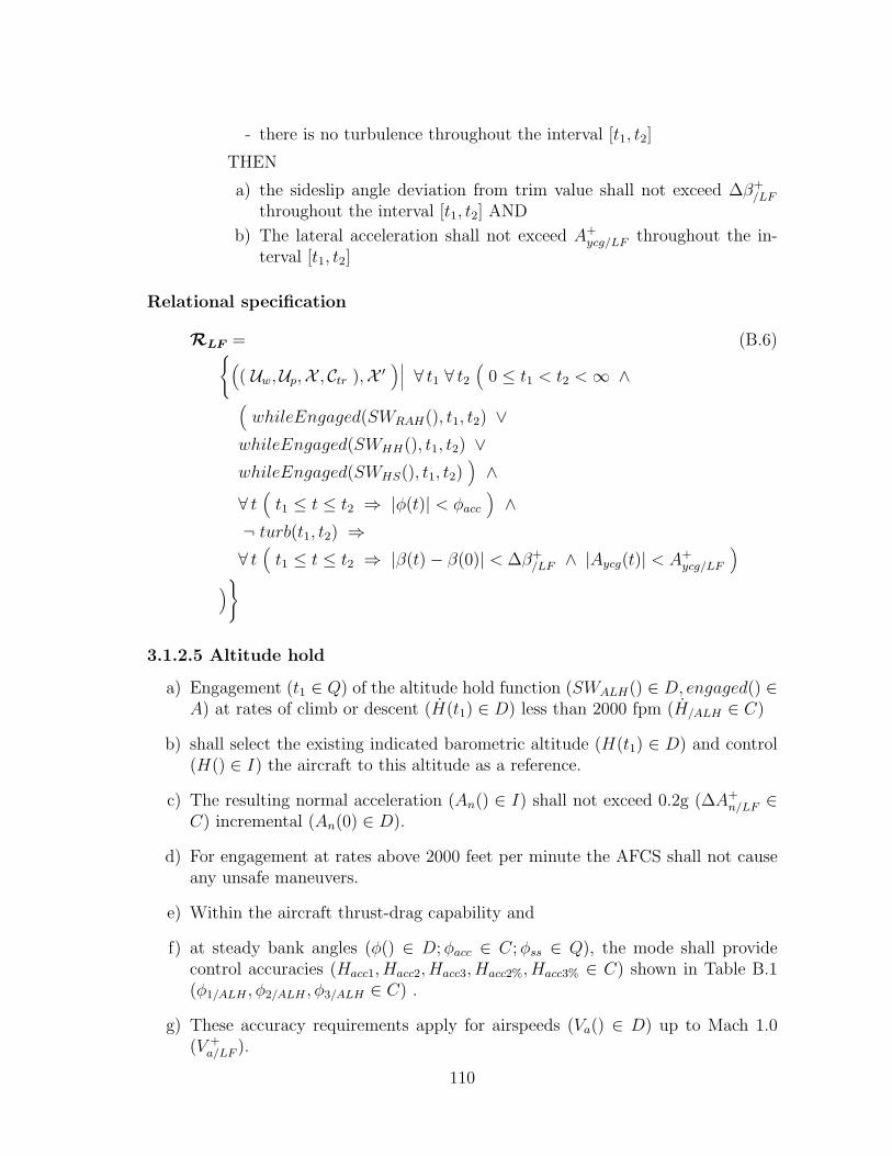
- there is no turbulence throughout the interval [t1, t2]
THEN
a) the sideslip angle deviation from trim value shall not exceed ∆β+/LF
throughout the interval [t1, t2] AND
b) The lateral acceleration shall not exceed A+ycg/LF throughout the in-
terval [t1, t2]
Relational specification
RLF = (B.6){(( Uw,Up,X , Ctr ),X ′
)∣∣∣ ∀ t1 ∀ t2(
0 ≤ t1 < t2 < ∞ ∧(whileEngaged(SWRAH(), t1, t2) ∨
whileEngaged(SWHH(), t1, t2) ∨whileEngaged(SWHS(), t1, t2)
)∧
∀ t(
t1 ≤ t ≤ t2 ⇒ |φ(t)| < φacc
)∧
¬ turb(t1, t2) ⇒∀ t
(t1 ≤ t ≤ t2 ⇒ |β(t) − β(0)| < ∆β+
/LF ∧ |Aycg(t)| < A+ycg/LF
))}
3.1.2.5 Altitude hold
a) Engagement (t1 ∈ Q) of the altitude hold function (SWALH() ∈ D, engaged() ∈A) at rates of climb or descent (H(t1) ∈ D) less than 2000 fpm (H/ALH ∈ C)
b) shall select the existing indicated barometric altitude (H(t1) ∈ D) and control(H() ∈ I) the aircraft to this altitude as a reference.
c) The resulting normal acceleration (An() ∈ I) shall not exceed 0.2g (∆A+n/LF ∈
C) incremental (An(0) ∈ D).
d) For engagement at rates above 2000 feet per minute the AFCS shall not causeany unsafe maneuvers.
e) Within the aircraft thrust-drag capability and
f) at steady bank angles (φ() ∈ D; φacc ∈ C; φss ∈ Q), the mode shall providecontrol accuracies (Hacc1, Hacc2, Hacc3, Hacc2%, Hacc3% ∈ C) shown in Table B.1(φ1/ALH , φ2/ALH , φ3/ALH ∈ C) .
g) These accuracy requirements apply for airspeeds (Va() ∈ D) up to Mach 1.0(V +
a/LF ).
110

h) Following engagement or perturbation of this mode at 2000 feet per minute orless, the specified accuracy shall be achieved within 30 seconds (TH ∈ C).
Table B.1: Minimum acceptable control accuracy for ALH function
Bank angle (deg.) 0 - 1 1 - 30 30 - 60
Alt. (ft.) 0 to 30000 ±30ft. ±60 ft or ±0.3%whichever islarger
±90 ft or ±0.4%whichever islarger
Intermediate specification
FOR EVERY couple of time instants t1, t2
IF
- [t1, t2] is a time interval within [0,∞) AND
- the length of the time interval [t1, t2] is larger than TH AND
a) the ALH control function is engaged at t = t1 and stays engagedthroughout the interval [t1, t2] AND
a) the rate of climb or descent at t = t1 is less than H/ALH AND
- the airplane is at a steady bank angle throughout the interval [t1, t2]AND
g) the airspeed is below V +a/LF AND
- there is no turbulence throughout the interval [t1, t2]
THEN
c) the normal acceleration deviation from trim value shall not exceed∆A+
n/LF throughout the interval [t1, t2] AND
b) f) h) throughout the interval [t1 + TH , t2] the airplane steady state bankangle is either less than φ1/ALH – in which case altitude deviationfrom H(t1) shall be less than Hacc1– OR the airplane steady state bankangle is within the interval [φ1/ALH , φ2/ALH ] – in which case altitudedeviation from H(t1) shall be less than the maximum between Hacc2
and Hacc2% ·H(t1) – OR the airplane steady state bank angle is withinthe interval [φ2/ALH , φ3/ALH ] – in which case altitude deviation fromH(t1) shall be less than the maximum between Hacc3 and Hacc3% ·H(t1)–.
111
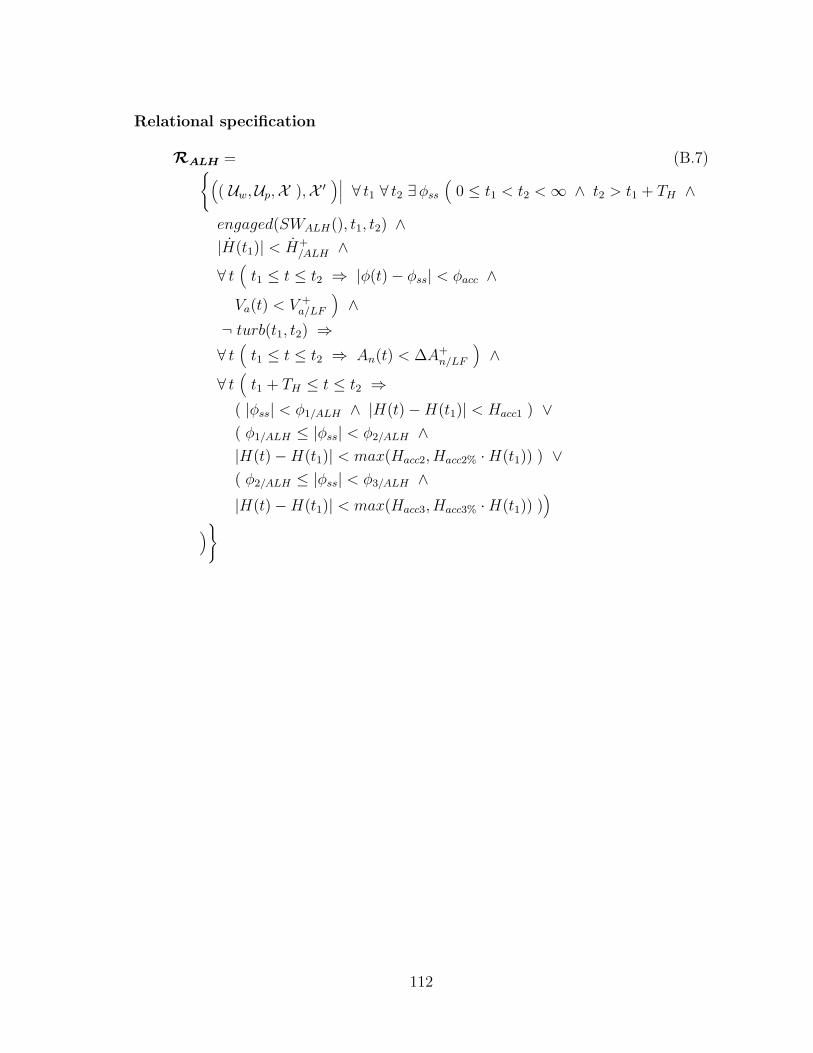
Relational specification
RALH = (B.7){(( Uw,Up,X ),X ′
)∣∣∣ ∀ t1 ∀ t2 ∃φss
(0 ≤ t1 < t2 < ∞ ∧ t2 > t1 + TH ∧
engaged(SWALH(), t1, t2) ∧|H(t1)| < H+
/ALH ∧∀ t
(t1 ≤ t ≤ t2 ⇒ |φ(t) − φss| < φacc ∧
Va(t) < V +a/LF
)∧
¬ turb(t1, t2) ⇒∀ t
(t1 ≤ t ≤ t2 ⇒ An(t) < ∆A+
n/LF
)∧
∀ t(
t1 + TH ≤ t ≤ t2 ⇒( |φss| < φ1/ALH ∧ |H(t) − H(t1)| < Hacc1 ) ∨( φ1/ALH ≤ |φss| < φ2/ALH ∧|H(t) − H(t1)| < max(Hacc2, Hacc2% · H(t1)) ) ∨( φ2/ALH ≤ |φss| < φ3/ALH ∧|H(t) − H(t1)| < max(Hacc3, Hacc3% · H(t1)) )
))}
112
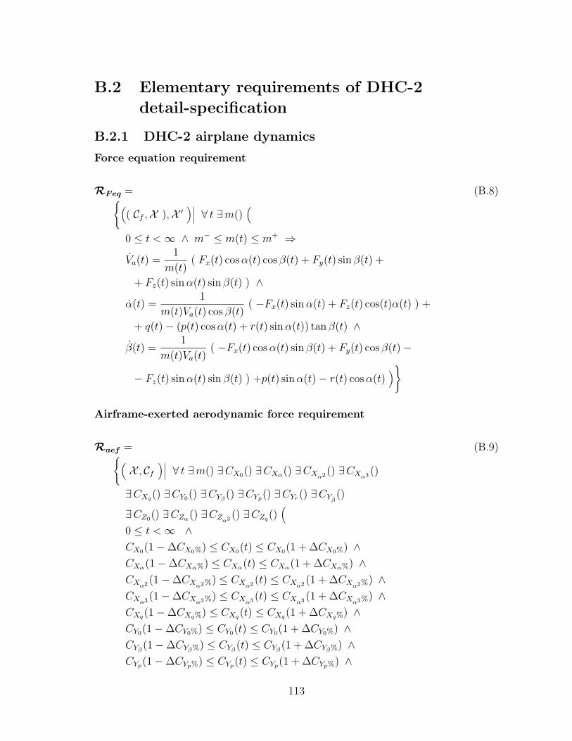
B.2 Elementary requirements of DHC-2
detail-specification
B.2.1 DHC-2 airplane dynamics
Force equation requirement
RFeq = (B.8){(( Cf ,X ),X ′
)∣∣∣ ∀ t ∃m()(
0 ≤ t < ∞ ∧ m− ≤ m(t) ≤ m+ ⇒Va(t) =
1
m(t)( Fx(t) cos α(t) cos β(t) + Fy(t) sin β(t) +
+ Fz(t) sin α(t) sin β(t) ) ∧α(t) =
1
m(t)Va(t) cos β(t)( −Fx(t) sin α(t) + Fz(t) cos(t)α(t) ) +
+ q(t) − (p(t) cos α(t) + r(t) sin α(t)) tan β(t) ∧β(t) =
1
m(t)Va(t)( −Fx(t) cos α(t) sin β(t) + Fy(t) cos β(t) −
− Fz(t) sin α(t) sin β(t) ) +p(t) sin α(t) − r(t) cos α(t))}
Airframe-exerted aerodynamic force requirement
Raef = (B.9){(X , Cf
)∣∣∣ ∀ t ∃m() ∃CX0() ∃CXα() ∃CXα2 () ∃CXα3 ()
∃CXq() ∃CY0() ∃CYβ() ∃CYp() ∃CYr() ∃CYβ
()
∃CZ0() ∃CZα() ∃CZα3 () ∃CZq()(
0 ≤ t < ∞ ∧CX0(1 − ∆CX0%) ≤ CX0(t) ≤ CX0(1 + ∆CX0%) ∧CXα(1 − ∆CXα%) ≤ CXα(t) ≤ CXα(1 + ∆CXα%) ∧CXα2 (1 − ∆CXα2%) ≤ CXα2 (t) ≤ CXα2 (1 + ∆CXα2%) ∧CXα3 (1 − ∆CXα3%) ≤ CXα3 (t) ≤ CXα3 (1 + ∆CXα3%) ∧CXq(1 − ∆CXq%) ≤ CXq(t) ≤ CXq(1 + ∆CXq%) ∧CY0(1 − ∆CY0%) ≤ CY0(t) ≤ CY0(1 + ∆CY0%) ∧CYβ
(1 − ∆CYβ%) ≤ CYβ(t) ≤ CYβ
(1 + ∆CYβ%) ∧CYp(1 − ∆CYp%) ≤ CYp(t) ≤ CYp(1 + ∆CYp%) ∧
113

CYr(1 − ∆CYr%) ≤ CYr(t) ≤ CYr(1 + ∆CYr%) ∧CYβ
(1 − ∆CYβ%) ≤ CYβ(t) ≤ CYβ
(1 + ∆CYβ%) ∧CZ0(1 − ∆CZ0%) ≤ CZ0(t) ≤ CZ0(1 + ∆CZ0%) ∧CZα(1 − ∆CZα%) ≤ CZα(t) ≤ CZα(1 + ∆CZα%) ∧CZα3 (1 − ∆CZα3%) ≤ CZα3 (t) ≤ CZα3 (1 + ∆CZα3%) ∧CZq(1 − ∆CZq%) ≤ CZq(t) ≤ CZq(1 + ∆CZq%) ⇒Xasd
(t) = qdyn(t)S(
CX0(t) + CXα(t)α(t) + CXα2 (t)α2(t) +
+ CXα3 (t)α3(t) + CXq(t)
c q(t)
Va(t)
)∧
Yasd(t) = qdyn(t)S
(CY0(t) + CYβ
(t)β(t) + CYp(t)b p(t)
2Va(t)+
+ CYr(t)b r(t)
2Va(t)+ CYβ
(t)bβ(t)
2Va(t)
)∧
Zasd(t) = qdyn(t)S
(CZ0(t) + CZα(t)α(t) + CZα3 (t)α
3(t) +
+ CZq(t)c q(t)
Va(t)
) )}
Moment equation requirement
RMeq = (B.10){(Cm,X
)∣∣∣ ∀ t ∃ Ix() ∃ Iy() ∃ Iz() ∃ Jxy() ∃ Jxz() ∃ Jyz()(
0 ≤ t < ∞ ∧Ix(1 − ∆Ix%) ≤ Ix(t) ≤ Ix ∧Iy(1 − ∆Iy%) ≤ Iy(t) ≤ Iy ∧Iz(1 − ∆Iz%) ≤ Iz(t) ≤ Iz ∧Jxy(1 − ∆Jxy%) ≤ Jxy(t) ≤ Jxy ∧Jxz(1 − ∆Jxz%) ≤ Jxz(t) ≤ Jxz ∧Jyz(1 − ∆Jyz%) ≤ Jyz(t) ≤ Jyz ⇒p(t) = Ppp(t)p
2(t) + Ppq(t)p(t)q(t) + Ppr(t)p(t)r(t) + Pqq(t)q2(t) +
+ Pqr(t)q(t)r(t) + Prr(t)r2(t) + Pl(t)L(t) + Pm(t)M(t) + Pn(t)N(t) ∧
q(t) = Qpp(t)p2(t) + Qpq(t)p(t)q(t) + Qpr(t)p(t)r(t) + Qqq(t)q
2(t) +
+ Qqr(t)q(t)r(t) + Qrr(t)r2(t) + Ql(t)L(t) + Qm(t)M(t) + Qn(t)N(t) ∧
r(t) = Rpp(t)p2(t) + Rpq(t)p(t)q(t) + Rpr(t)p(t)r(t) + Rqq(t)q
2(t) +
+ Rqr(t)q(t)r(t) + Rrr(t)r2(t) + Rl(t)L(t) + Rm(t)M(t) + Rn(t)N(t)
)}
114

Airframe-exerted aerodynamic moment requirement
Raem = (B.11){(X , Cm
)∣∣∣ ∀ t ∃m() ∃Cl0() ∃Clβ() ∃Clp() ∃Clr() ∃Cmα() ∃Cmα2 () ∃Cmq()
∃Cmβ2 () ∃Cmr() ∃Cn0() ∃Cnβ3 () ∃Cnβ() ∃Cnp() ∃Cnr() ∃Cnq()
(0 ≤ t < ∞ ∧Cl0(1 − ∆Cl0%) ≤ Cl0(t) ≤ Cl0(1 + ∆Cl0%) ∧Clβ(1 − ∆Clβ%) ≤ Clβ(t) ≤ Clβ(1 + ∆Clβ%) ∧Clp(1 − ∆Clp%) ≤ Clp(t) ≤ Clp(1 + ∆Clp%) ∧Clr(1 − ∆Clr%) ≤ Clr(t) ≤ Clr(1 + ∆Clr%) ∧Cm0(1 − ∆Cm0%) ≤ Cm0(t) ≤ Cm0(1 + ∆Cm0%) ∧Cm−
α≤ Cmα(t) ≤ Cm+
α∧
Cmα2 (1 − ∆Cmα2%) ≤ Cmα2 (t) ≤ Cmα2 (1 + ∆Cmα2%) ∧Cmq(1 − ∆Cmq%) ≤ Cmq(t) ≤ Cmq(1 + ∆Cmq%) ∧Cmβ2 (1 − ∆Cmβ2%) ≤ Cmβ2 (t) ≤ Cmβ2 (1 + ∆Cmβ2%) ∧Cmr(1 − ∆Cmr%) ≤ Cmr(t) ≤ Cmr(1 + ∆Cmr%) ∧Cn0(1 − ∆Cn0%) ≤ Cn0(t) ≤ Cn0(1 + ∆Cn0%) ∧Cnβ
(1 − ∆Cnβ%) ≤ Cnβ(t) ≤ Cnβ
(1 + ∆Cnβ%) ∧Cnp(1 − ∆Cnp%) ≤ Cnp(t) ≤ Cnp(1 + ∆Cnp%) ∧Cnr(1 − ∆Cnr%) ≤ Cnr(t) ≤ Cnr(1 + ∆Cnr%) ∧Cnq(1 − ∆Cnq%) ≤ Cnq(t) ≤ Cnq(1 + ∆Cnq%) ∧Cnβ3 (1 − ∆Cnβ3%) ≤ Cnβ3 (t) ≤ Cnβ3 (1 + ∆Cnβ3%) ⇒
Lasd(t) = qdyn(t)S
b
2
(Cl0(t) + Clβ(t)β(t) + Clp(t)
b p(t)
2Va(t)+
+ Clr(t)b r(t)
2Va(t)
)∧
Masd(t) = qdyn(t)Sc
(Cm0(t) + Cmα(t)α(t) + Cmα2 (t)α
2(t) +
+ Cmq(t)c q(t)
Va(t)+ Cmβ2 (t)β
2(t) + Cmr(t)b r(t)
2Va(t)
)∧
Nasd(t) = qdyn(t)S
b
2
(Cn0(t) + Cnβ
(t)β(t) + Cnp(t)b p(t)
2Va(t)+
+ Cnr(t)b r(t)
2Va(t)+ Cnq(t)
c q(t)
V (t)+ Cnβ3 (t)β
3(t)) )}
115

Kinematic equation requirement
RKeq = (B.12){(X ,X ′
)∣∣∣ ∀ t(
0 ≤ t < ∞ ⇒
ψ(t) =q(t) sin φ(t) + r(t) cos φ(t)
cosθ(t)∧
θ(t) = q(t) cos φ(t) − r(t) sin φ(t) ∧φ(t) = p(t) + (q(t) sin φ(t) + r(t) cos φ(t)) tan θ(t)
)}
Navigation equation requirement
RNeq = (B.13){(( Uw,X ),X
)∣∣∣ ∀ t(
0 ≤ t < ∞ ⇒
H(t) = ue(t) sin θ(t)+ ( ve(t) sin φ(t) + we(t) cos φ(t) ) cos θ(t))}
Gravity force requirement
Rgrf = (B.14){(X , Cf
)∣∣∣ ∀ t ∃m()(
0 ≤ t < ∞ ∧ m− ≤ m(t) ≤ m+ ⇒Xgr(t) = −m(t)g0 sin θ(t) ∧Ygr(t) = m(t)g0 cos θ(t) sin φ(t) ∧Zgr(t) = m(t)g0 cos θ(t) cos φ(t)
)}
Wind Force requirement
Rwf = (B.15){(( Uw,X ), Cf
)∣∣∣ ∀ t ∃m()(
0 ≤ t < ∞ ∧ m− ≤ m(t) ≤ m+ ⇒Xw(t) = −m(t)(uw(t) + q(t)ww(t) − r(t)vw(t)) ∧Yw(t) = −m(t)(vw(t) − p(t)ww(t) + r(t)uw(t)) ∧Zw(t) = −m(t)(ww(t) + p(t)vw(t) − q(t)uw(t))
)}
116

Control-surface-exerted aerodynamic force requirement
Rcsf = (B.16){(( Uc,X ), Cf
)∣∣∣ ∀ t ∃CXδr() ∃CXδf
() ∃CXαδf() ∃CYδa
() ∃CYδr() ∃CYαδr
()
∃CZδe() ∃CZβ2δe
() ∃CZδf() ∃CZαδf
()(
0 ≤ t < ∞ ∧CXδr
(1 − ∆CXδr%) ≤ CXδr(t) ≤ CXδr
(1 + ∆CXδr%) ∧CXδf
(1 − ∆CXδf%) ≤ CXδf(t) ≤ CXδf
(1 + ∆CXδf%) ∧CXαδf
(1 − ∆CXαδf%) ≤ CXαδf(t) ≤ CXαδf
(1 + ∆CXαδf%) ∧CYδa
(1 − ∆CYδa%) ≤ CYδa(t) ≤ CYδa
(1 + ∆CYδa%) ∧CYδr
(1 − ∆CYδr%) ≤ CYδr(t) ≤ CYδr
(1 + ∆CYδr%) ∧CYαδr
(1 − ∆CYαδr%) ≤ CYαδr(t) ≤ CYαδr
(1 + ∆CYαδr%) ∧CZδe
(1 − ∆CZδe%) ≤ CZδe(t) ≤ CZδe
(1 + ∆CZδe%) ∧CZβ2δe
(1 − ∆CZβ2δe%) ≤ CZβ2δe
(t) ≤ CZβ2δe(1 + ∆CZβ2δe%
) ∧CZδf
(1 − ∆CZδf%) ≤ CZδf(t) ≤ CZδf
(1 + ∆CZδf%) ∧CZαδf
(1 − ∆CZαδf%) ≤ CZαδf(t) ≤ CZαδf
(1 + ∆CZαδf%) ⇒Xacd
(t) = qdyn(t)S ( CXδr(t)δr(t) + CXδf
(t)δf (t) + CXαδf(t)α(t)δf (t) ) ∧
Yacd(t) = qdyn(t)S ( CYδa
(t)δa(t) + CYδr(t)δr(t) + CYαδr
(t)α(t)δr(t) ) ∧Zacd
(t) = qdyn(t)S ( CZδe(t)δe(t) + CZβ2δe
(t)β2(t)δe(t) + CZδf (t)δf (t) ))}
Control-surface-exerted aerodynamic moment requirement
Rcsm = (B.17){(( Uc,X ), Cm
)∣∣∣ ∀ t ∃Clδa() ∃Clδr
() ∃Clαδa() ∃Cmδe
() Cmδf()
∃Cnδa() ∃Cnδr
()(
0 ≤ t < ∞ ∧Clδa
(1 − ∆Clδa%) ≤ Clδa(t) ≤ Clδa
(1 + ∆Clδa%) ∧Clδr
(1 − ∆Clδr%) ≤ Clδr(t) ≤ Clδr
(1 + ∆Clδr%) ∧Clαδa
(1 − ∆Clαδa%) ≤ Clαδa(t) ≤ Clαδa
(1 + ∆Clαδa) ∧
Cmδe(1 − ∆Cmδe%) ≤ Cmδe
(t) ≤ Cmδe(1 + ∆Cmδe%) ∧
Cmδf(1 − ∆Cmδf%) ≤ Cmδf
(t) ≤ Cmδf(1 + ∆Cmδf%) ∧
Cnδa(1 − ∆Cnδa%) ≤ Cnδa
(t) ≤ Cnδa(1 + ∆Cnδa%) ∧
Cnδr(1 − ∆Cnδr%) ≤ Cnδr
(t) ≤ Cnδr(1 + ∆Cnδr%) ⇒
Lacd(t) = qdyn(t)S
b
2( Clδa
(t)δa(t) + Clδr(t)δr(t) + Clαδa(t)α(t)δa(t) ) ∧
117
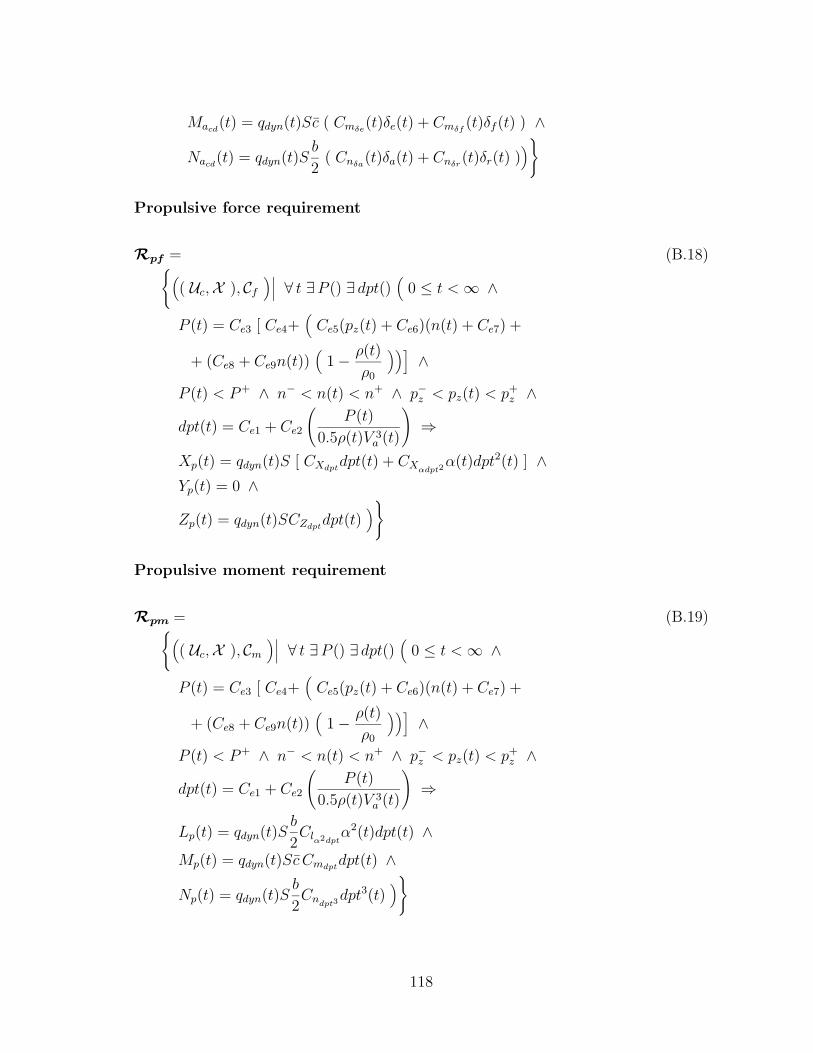
Macd(t) = qdyn(t)Sc ( Cmδe
(t)δe(t) + Cmδf(t)δf (t) ) ∧
Nacd(t) = qdyn(t)S
b
2( Cnδa
(t)δa(t) + Cnδr(t)δr(t) )
)}
Propulsive force requirement
Rpf = (B.18){(( Uc,X ), Cf
)∣∣∣ ∀ t ∃P () ∃ dpt()(
0 ≤ t < ∞ ∧
P (t) = Ce3 [ Ce4+(
Ce5(pz(t) + Ce6)(n(t) + Ce7) +
+ (Ce8 + Ce9n(t))(
1 − ρ(t)
ρ0
))]∧
P (t) < P+ ∧ n− < n(t) < n+ ∧ p−z < pz(t) < p+z ∧
dpt(t) = Ce1 + Ce2
(P (t)
0.5ρ(t)V 3a (t)
)⇒
Xp(t) = qdyn(t)S [ CXdptdpt(t) + CXαdpt2
α(t)dpt2(t) ] ∧Yp(t) = 0 ∧Zp(t) = qdyn(t)SCZdpt
dpt(t))}
Propulsive moment requirement
Rpm = (B.19){(( Uc,X ), Cm
)∣∣∣ ∀ t ∃P () ∃ dpt()(
0 ≤ t < ∞ ∧
P (t) = Ce3 [ Ce4+(
Ce5(pz(t) + Ce6)(n(t) + Ce7) +
+ (Ce8 + Ce9n(t))(
1 − ρ(t)
ρ0
))]∧
P (t) < P+ ∧ n− < n(t) < n+ ∧ p−z < pz(t) < p+z ∧
dpt(t) = Ce1 + Ce2
(P (t)
0.5ρ(t)V 3a (t)
)⇒
Lp(t) = qdyn(t)Sb
2Clα2dpt
α2(t)dpt(t) ∧Mp(t) = qdyn(t)Sc Cmdpt
dpt(t) ∧
Np(t) = qdyn(t)Sb
2Cndpt3
dpt3(t))}
118

Kinematic acceleration at crew station requirement
Rka = (B.20){(( Uw,X ),X ′
)∣∣∣ ∀ t(
0 ≤ t < ∞ ⇒Ax(t) = ue(t) + q(t)we(t) − r(t)ve(t) + q(t)rz − r(t)ry +
+ p(t)q(t)ry + p(t)r(t)rz − q2(t)rx − r2(t)rx ∧Ay(t) = ve(t) + r(t)ue(t) − p(t)we(t) + r(t)rx − p(t)rz +
+ p(t)q(t)rx + q(t)r(t)rz − p2(t)ry − r2(t)ry ∧Az(t) = we(t) + p(t)ve(t) − q(t)ue(t) + p(t)ry − q(t)rx +
+ p(t)r(t)rx + q(t)r(t)ry − p2(t)rz − q2(t)rz
)}
Air data requirement
Rad = (B.21){(X ,X ′
)∣∣∣ ∀ t(
0 ≤ t < ∞ ⇒T (t) = T0 + λH(t) ∧
ps(t) = p0
(T0
T (t)
) g0λR
∧
ρ(t) =ps(t)
RT (t)∧
qdyn(t) = 0.5ρ(t)V 2a (t)
)}
B.2.2 DHC-2 Flight Control System Hardware
Rudder actuator
Rrud = (B.22){(( X , Uc ),Uc
)∣∣∣ ∀ t ∃xr()(
0 ≤ t < ∞ ∧
xr(0) = −A−1r Brur(0) ∧
xr(t) = Arxr(t) + Brur(t) ⇒δr(t) = Crxr(t) + Drur(t)
)}
119

Aileron actuator
Rail = (B.23){(( X , Uc ),Uc
)∣∣∣ ∀ t ∃xa()(
0 ≤ t < ∞ ∧
xa(0) = −A−1a Baua(0) ∧
xa(t) = Aaxa(t) + Baua(t) ⇒δa(t) = 2Caxa(t) + Daua(t)
)}
Elevator actuator
Relv = (B.24){(( X , Uc ),Uc
)∣∣∣ ∀ t ∃xe()(
0 ≤ t < ∞ ∧
xe(0) = −A−1e Beue(0) ∧
xe(t) = Aexe(t) + Beue(t) ⇒δe(t) = Cexe(t) + Deue(t)
)}
Roll rate gyro requirement
Rp = (B.25){(X , X
)∣∣∣ ∀ t ∃Sp ∃ biasp ∃ νp()(
0 ≤ t < ∞ ∧S−
g ≤ Sp ≤ S+g ∧
BIAS−g ≤ biasp ≤ BIAS+
g ∧whiteNoise(νp(), Npsdg) ⇒p(t) '
[Sp [ p(t) ]
IR+g
IR−g
+biasp + νp(t)]OR+
g
OR−g
)}
Pitch rate gyro requirement
Rq = (B.26){(X , X
)∣∣∣ ∀ t ∃Sq ∃ biasq ∃ νq()(
0 ≤ t < ∞ ∧S−
g ≤ Sq ≤ S+g ∧
BIAS−g ≤ biasq ≤ BIAS+
g ∧
120

whiteNoise(νq(), Npsdg) ⇒q(t) '
[Sq [ q(t) ]
IR+g
IR−g
+biasq + νq(t)]OR+
g
OR−g
)}
Yaw rate gyro requirement
Rr = (B.27){(X , X
)∣∣∣ ∀ t ∃Sr ∃ biasr ∃ νr()(
0 ≤ t < ∞ ∧S−
g ≤ Sr ≤ S+g ∧
BIAS−g ≤ biasr ≤ BIAS+
g ∧whiteNoise(νr(), Npsdg) ⇒r(t) '
[Sr [ r(t) ]
IR+g
IR−g
+biasr + νr(t)]OR+
g
OR−g
)}
Angle of attack sensor requirement
Rα = (B.28){(X , X
)∣∣∣ ∀ t ∃Sα ∃ biasα ∃ να()(
0 ≤ t < ∞ ∧S−
α ≤ Sα ≤ S+α ∧
BIAS−α ≤ biasα ≤ BIAS+
α ∧whiteNoise(να(), Npsdα) ⇒α(t) '
[Sα [ α(t) ]IR+
α
IR−α
+biasα + να(t)]OR+
α
OR−α
)}
Ax accelerometer requirement
RAx = (B.29){(X , X
)∣∣∣ ∀ t ∃SAx ∃ biasAx ∃ νAx()(
0 ≤ t < ∞ ∧S−
A ≤ SAx ≤ S+A ∧
BIAS−A ≤ biasAx ≤ BIAS+
A ∧whiteNoise(νAx(), NpsdA) ⇒Ax(t) '
[SAx [ Ax(t) + sin θ(t) ]
IR+A
IR−A
+biasAx + νAx(t)]OR+
A
OR−A
)}
121

Ay accelerometer requirement
RAy = (B.30){(X , X
)∣∣∣ ∀ t ∃SAy ∃ biasAy ∃ νAy()(
0 ≤ t < ∞ ∧S−
A ≤ SAy ≤ S+A ∧
BIAS−A ≤ biasAy ≤ BIAS+
A ∧whiteNoise(νAy(), NpsdA) ⇒Ay(t) '
[SAy [ Ay(t) − cos θ(t) sin φ(t) ]
IR+A
IR−A
+biasAy + νAy(t)]OR+
A
OR−A
)}
Az accelerometer requirement
RAz = (B.31){(X , X
)∣∣∣ ∀ t ∃SAz ∃ biasAz ∃ νAz()(
0 ≤ t < ∞ ∧S−
A ≤ SAz ≤ S+A ∧
BIAS−A ≤ biasAz ≤ BIAS+
A ∧whiteNoise(νAz(), NpsdA) ⇒Az(t) '
[SAz [ Az(t) + cos θ(t) sin φ(t) ]
IR+A
IR−A
+biasAz + νAz(t)]OR+
A
OR−A
)}
Dynamic pressure sensor requirement
Rqdyn= (B.32){(X , X
)∣∣∣ ∀ t ∃Sqdyn∃ biasqdyn
∃ νqdyn()
(0 ≤ t < ∞ ∧
S−qdyn
≤ Sqdyn≤ S+
qdyn∧
BIAS−qdyn
≤ biasqdyn≤ BIAS+
qdyn∧
whiteNoise(νqdyn(), Npsdqdyn
) ⇒
qdyn(t) '[
Sqdyn[ qdyn(t) ]
IR+qdyn
IR−qdyn
+biasqdyn+ νqdyn
(t)]OR+
qdyn
OR−qdyn
)}
Static pressure sensor requirement
Rps = (B.33){(X , X
)∣∣∣ ∀ t ∃Sps ∃ biasps ∃ νps()(
0 ≤ t < ∞ ∧
122
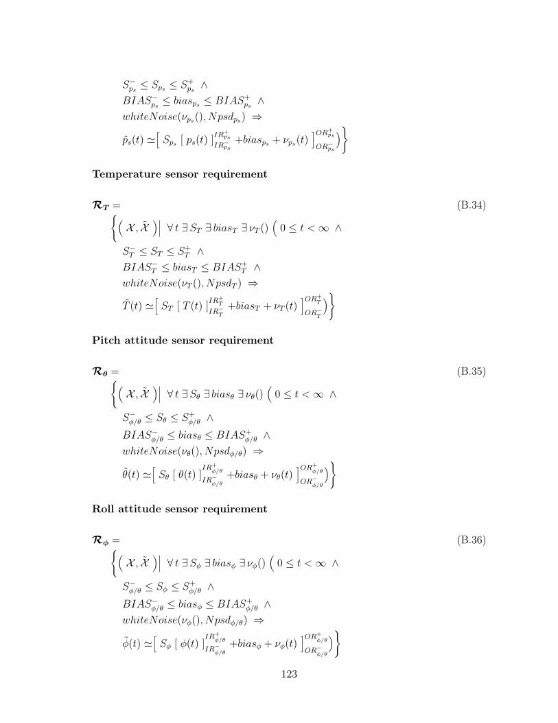
S−ps
≤ Sps ≤ S+ps
∧BIAS−
ps≤ biasps ≤ BIAS+
ps∧
whiteNoise(νps(), Npsdps) ⇒ps(t) '
[Sps [ ps(t) ]
IR+ps
IR−ps
+biasps + νps(t)]OR+
ps
OR−ps
)}
Temperature sensor requirement
RT = (B.34){(X , X
)∣∣∣ ∀ t ∃ST ∃ biasT ∃ νT ()(
0 ≤ t < ∞ ∧S−
T ≤ ST ≤ S+T ∧
BIAS−T ≤ biasT ≤ BIAS+
T ∧whiteNoise(νT (), NpsdT ) ⇒T (t) '
[ST [ T (t) ]
IR+T
IR−T
+biasT + νT (t)]OR+
T
OR−T
)}
Pitch attitude sensor requirement
Rθ = (B.35){(X , X
)∣∣∣ ∀ t ∃Sθ ∃ biasθ ∃ νθ()(
0 ≤ t < ∞ ∧S−
φ/θ ≤ Sθ ≤ S+φ/θ ∧
BIAS−φ/θ ≤ biasθ ≤ BIAS+
φ/θ ∧whiteNoise(νθ(), Npsdφ/θ) ⇒θ(t) '
[Sθ [ θ(t) ]
IR+φ/θ
IR−φ/θ
+biasθ + νθ(t)]OR+
φ/θ
OR−φ/θ
)}
Roll attitude sensor requirement
Rφ = (B.36){(X , X
)∣∣∣ ∀ t ∃Sφ ∃ biasφ ∃ νφ()(
0 ≤ t < ∞ ∧S−
φ/θ ≤ Sφ ≤ S+φ/θ ∧
BIAS−φ/θ ≤ biasφ ≤ BIAS+
φ/θ ∧whiteNoise(νφ(), Npsdφ/θ) ⇒φ(t) '
[Sφ [ φ(t) ]
IR+φ/θ
IR−φ/θ
+biasφ + νφ(t)]OR+
φ/θ
OR−φ/θ
)}
123

Heading sensor requirement
Rψ = (B.37){(X , X
)∣∣∣ ∀ t ∃Sψ ∃ biasψ ∃ νψ()(
0 ≤ t < ∞ ∧S−
ψ ≤ Sψ ≤ S+ψ ∧
BIAS−ψ ≤ biasψ ≤ BIAS+
ψ ∧whiteNoise(νψ(), Npsdψ) ⇒ψ(t) '
[Sψ [ ψ(t) ]
IR+ψ
IR−ψ
+biasψ + νψ(t)]OR+
ψ
OR−ψ
)}
DAC card requirement
RDAC = (B.38){(Uc, Uc
)∣∣∣ ∀ k ∀ t(
0 ≤ k < ∞ ∧ kTs ≤ t < (k + 1)Ts ⇒δe(t) = (δe(k) − OFFDAC)S−1
DAC ∧δa(t) = (δa(k) − OFFDAC)S−1
DAC ∧δr(t) = (δr(k) − OFFDAC)S−1
DAC
)}
ADC card requirement
RADC = (B.39){(( Up, X ), ( Up, X )
)∣∣∣ ∀ k(
0 ≤ k < ∞ ⇒
p(k) =⌊
SADC [ p(k Ts) ]ADCV +
ADCV − +OFFADC
⌋∧
q(k) =⌊
SADC [ q(k Ts) ]ADCV +
ADCV − +OFFADC
⌋∧
r(k) =⌊
SADC [ r(k Ts) ]ADCV +
ADCV − +OFFADC
⌋∧
α(k) =⌊
SADC [ α(k Ts) ]ADCV +
ADCV − +OFFADC
⌋∧
Ax(k) =⌊
SADC [ Ax(k Ts) ]ADCV +
ADCV − +OFFADC
⌋∧
Ay(k) =⌊
SADC [ Ay(k Ts) ]ADCV +
ADCV − +OFFADC
⌋∧
Az(k) =⌊
SADC [ Az(k Ts) ]ADCV +
ADCV − +OFFADC
⌋∧
ψ(k) =⌊
SADC [ ψ(k Ts) ]ADCV +
ADCV − +OFFADC
⌋∧
θ(k) =⌊
SADC [ θ(k Ts) ]ADCV +
ADCV − +OFFADC
⌋∧
124

φ(k) =⌊
SADC [ φ(k Ts) ]ADCV +
ADCV − +OFFADC
⌋∧
qdyn(k) =⌊
SADC [ qdyn(k Ts) ]ADCV +
ADCV − +OFFADC
⌋∧
ps(k) =⌊
SADC [ ps(k Ts) ]ADCV +
ADCV − +OFFADC
⌋∧
T (k) =⌊
SADC [ T (k Ts) ]ADCV +
ADCV − +OFFADC
⌋∧
φr(k) =⌊
SADC [ φr(k Ts) ]ADCV +
ADCV − +OFFADC
⌋∧
ψr(k) =⌊
SADC [ ψr(k Ts) ]ADCV +
ADCV − +OFFADC
⌋∧
θr(k) =⌊
SADC [ θr(k Ts) ]ADCV +
ADCV − +OFFADC
⌋∧
¯SW PAH(k) =⌊
SADC [ SW PAH(k Ts) ]ADCV +
ADCV − +OFFADC
⌋∧
¯SWALH(k) =⌊
SADC [ SWALH(k Ts) ]ADCV +
ADCV − +OFFADC
⌋∧
¯SWRAH(k) =⌊
SADC [ SWRAH(k Ts) ]ADCV +
ADCV − +OFFADC
⌋∧
¯SWHH(k) =⌊
SADC [ SWHH(k Ts) ]ADCV +
ADCV − +OFFADC
⌋∧
¯SWHS(k) =⌊
SADC [ SWHS(k Ts) ]ADCV +
ADCV − +OFFADC
⌋)}
Control panel requirement
RCP = (B.40){(Up, Up
)∣∣∣ ∀ t(
0 ≤ t < ∞ ⇒
(SW PAH(t) > Vth ⇔ SWPAH(t) = ON) ∧(SWALH(t) > Vth ⇔ SWALH(t) = ON) ∧(SWRAH(t) > Vth ⇔ SWRAH(t) = ON) ∧(SWHH(t) > Vth ⇔ SWHH(t) = ON) ∧(SWHS(t) > Vth ⇔ SWHS(t) = ON) ∧θr(t) = Sθrθr(t) + BIASθr ∧φr(t) = Sφrφr(t) + BIASφr ∧ψr(t) = Sψrψr(t) + BIASψr
)}
125
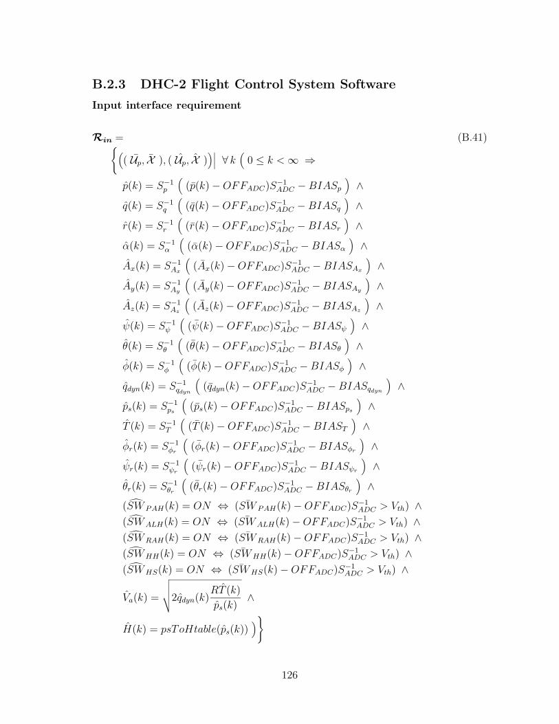
B.2.3 DHC-2 Flight Control System Software
Input interface requirement
Rin = (B.41){(( Up, X ), ( Up, X )
)∣∣∣ ∀ k(
0 ≤ k < ∞ ⇒
p(k) = S−1p
((p(k) − OFFADC)S−1
ADC − BIASp
)∧
q(k) = S−1q
((q(k) − OFFADC)S−1
ADC − BIASq
)∧
r(k) = S−1r
((r(k) − OFFADC)S−1
ADC − BIASr
)∧
α(k) = S−1α
((α(k) − OFFADC)S−1
ADC − BIASα
)∧
Ax(k) = S−1Ax
((Ax(k) − OFFADC)S−1
ADC − BIASAx
)∧
Ay(k) = S−1Ay
((Ay(k) − OFFADC)S−1
ADC − BIASAy
)∧
Az(k) = S−1Az
((Az(k) − OFFADC)S−1
ADC − BIASAz
)∧
ψ(k) = S−1ψ
((ψ(k) − OFFADC)S−1
ADC − BIASψ
)∧
θ(k) = S−1θ
((θ(k) − OFFADC)S−1
ADC − BIASθ
)∧
φ(k) = S−1φ
((φ(k) − OFFADC)S−1
ADC − BIASφ
)∧
qdyn(k) = S−1qdyn
((qdyn(k) − OFFADC)S−1
ADC − BIASqdyn
)∧
ps(k) = S−1ps
((ps(k) − OFFADC)S−1
ADC − BIASps
)∧
T (k) = S−1T
((T (k) − OFFADC)S−1
ADC − BIAST
)∧
φr(k) = S−1φr
((φr(k) − OFFADC)S−1
ADC − BIASφr
)∧
ψr(k) = S−1ψr
((ψr(k) − OFFADC)S−1
ADC − BIASψr
)∧
θr(k) = S−1θr
((θr(k) − OFFADC)S−1
ADC − BIASθr
)∧
(SW PAH(k) = ON ⇔ ( ¯SW PAH(k) − OFFADC)S−1ADC > Vth) ∧
(SWALH(k) = ON ⇔ ( ¯SWALH(k) − OFFADC)S−1ADC > Vth) ∧
(SWRAH(k) = ON ⇔ ( ¯SWRAH(k) − OFFADC)S−1ADC > Vth) ∧
(SWHH(k) = ON ⇔ ( ¯SWHH(k) − OFFADC)S−1ADC > Vth) ∧
(SWHS(k) = ON ⇔ ( ¯SWHS(k) − OFFADC)S−1ADC > Vth) ∧
Va(k) =
√√√√2qdyn(k)RT (k)
ps(k)∧
H(k) = psToHtable(ps(k)))}
126

Output interface requirement
Rout = (B.42){(Uc, Uc
)∣∣∣ ∀ k(
0 ≤ k < ∞ ⇒
δe(k) =⌊
SDAC
[δe(k)
]DACV +
DACV −+OFFDAC
⌋∧
δa(k) =⌊
SDAC
[δa(k)
]DACV +
DACV −+OFFDAC
⌋∧
δr(k) =⌊
SDAC
[δr(k)
]DACV +
DACV −+OFFDAC
⌋)}
Pitch Attitude Hold FCL requirement
RPAH
= (B.43){(( Up, X ), Uc
)∣∣∣ ∀ k(
1 ≤ k < ∞ ∧ SW PAH(k) = ON ⇒
∆δe(k) =[(
[ ∆θr(k) ]∆θ+r
∆θ−r−∆θ(k)
)Kθ(Va)
]∆θ+V
∆θ−V−
−(
q(k) − r(k) tan φ(k) − Ktc(Va)(sec(φ(k) + ∆φPAH) − 1))
Kq(Va) +
+[[(
[ ∆θr(k) ]∆θ+r
∆θ−r−∆θ(k)
)Kθ(Va)
]∆θ+V
∆θ−VKs i
Ts
z − 1
]l+s1
l−s1
)}
Altitude Hold FCL requirement
RALH
= (B.44){(( Up, X ), Uc
)∣∣∣ ∀ k1 ∀ k2
(1 ≤ k1 < k2 < ∞ ∧
engaged(SWALH(), k1, k2) ⇒∀ k
(1 ≤ k < ∞ ∧ SWALH(k) = ON ⇒
∆δe(k) =[(
[( ∆H(k1) − ∆H(k) ) KH(Va)K−1θ (Va) ]∆θ+
r
∆θ−r+
−([
Kd(Va)Ts
z − 1 + Kd(Va)Ts
∆θ(k) ]l+s1l−s1
+∆θ(k)))
Kθ(Va)]∆θ+
V
∆θ−V
−(
q(k) − r(k) tan φ(k) − Ktc(Va)(sec(φ(k) + ∆φAL) − 1))
Kq(Va)
+[[(
[( ∆H(k1) − ∆H(k) ) KH(Va)K−1θ (Va) ]∆θ+
r
∆θ−r
−([
Kd(Va)Ts
z − 1 + Kd(Va)Ts
∆θ(k) ]l+s2l−s2
+∆θ(k)))
Kθ(Va)]∆θ+
V
∆θ−V·
127

·Ks iTs
z − 1
]l+s1
l−s1
)}
Roll Attitude Hold FCL requirement
RRAH
= (B.45){(( Up, X ), Uc
)∣∣∣ ∀ k(
1 ≤ k < ∞ ∧ SWRAH(k) = ON ⇒
∆δa(k) =[(
[ ∆φr(k) ]∆φ+r
∆φ−r−∆φ(k)
)Kφ(Va)
]∆φ+V
∆φ−V
+dar · r(k) +
+[[(
[ ∆φr(k) ]∆φ+r
∆φ−r−∆φ(k)
)Kφ(Va)
]∆φ+V
∆φ−V
Ka iTs
z − 1
]l+a
l−a∧
∆δr(k) = Krg0
Va(k)sin φ(k) + (drr(Va) − Kr)r(k)
)}
Heading Select FCL requirement
RHS
= (B.46){(( Up, X ), Uc
)∣∣∣ ∀ k(
1 ≤ k < ∞ ∧ SWHS(k) = ON ⇒
∆δa(k) =[(
[( ∆ψr(k) − ∆ψ(k) ) Kψ(Va) ]∆φ+r
∆φ−r−
− ∆φ(k))
Kφ(Va)]∆φ+
V
∆φ−V
+dar · r(k) +
+[[(
[( ∆ψr(k) − ∆ψ(k) ) Kψ(Va) ]∆φ+r
∆φ−r−∆φ(k)
)Kφ(Va)
]∆φ+V
∆φ−V
·
·Ka iTs
z − 1
]l+a
l−a∧
∆δr(k) = Krg0
Va(k)sin φ(k) + (drr(Va) − Kr)r(k)
)}
Heading Hold FCL requirement
RHH
= (B.47){(( Up, X ), Uc
)∣∣∣ ∀ k1 ∀ k2
(1 ≤ k1 < k2 < ∞ ∧
engaged(SWHH(), k1, k2) ⇒∀ k
(∆δa(k) =
[([( ∆ψ(k1) − ∆ψ(k) ) Kψ(Va) ]∆φ+
r
∆φ−r−
− ∆φ(k))
Kφ(Va)]∆φ+
V
∆φ−V
+dar · r(k) +
128

+[[(
[( ∆ψ(k1) − ∆ψ(k) ) Kψ(Va) ]∆φ+r
∆φ−r−∆φ(k)
)Kφ(Va)
]∆φ+V
∆φ−V
·
·Ka iTs
z − 1
]l+a
l−a∧
∆δr(k) = Krg0
Va(k)sin φ(k) + (drr(Va) − Kr)r(k)
))}
129

B.3 Fault modes
B.3.1 Control-surface fault modes
Partial loss of rudder surface
Rcsf,1 = (B.48){(( Uc,X ), Cf
)∣∣∣ ∀ t ∃CXδr() ∃CXδf
() ∃CXαδf() ∃CYδa
() ∃CYδr() ∃CYαδr
()
∃CZδe() ∃CZβ2δe
() ∃CZδf() ∃CZαδf
() ∃ loss(
0 ≤ t < ∞ ∧ 0 < loss ≤ 1 ∧CXδr
(1 − ∆CXδr%) ≤ CXδr(t) ≤ CXδr
(1 + ∆CXδr%) ∧CXδf
(1 − ∆CXδf%) ≤ CXδf(t) ≤ CXδf
(1 + ∆CXδf%) ∧CXαδf
(1 − ∆CXαδf%) ≤ CXαδf(t) ≤ CXαδf
(1 + ∆CXαδf%) ∧CYδa
(1 − ∆CYδa%) ≤ CYδa(t) ≤ CYδa
(1 + ∆CYδa%) ∧CYδr
(1 − ∆CYδr%) ≤ CYδr(t) ≤ CYδr
(1 + ∆CYδr%) ∧CYαδr
(1 − ∆CYαδr%) ≤ CYαδr(t) ≤ CYαδr
(1 + ∆CYαδr%) ∧CZδe
(1 − ∆CZδe%) ≤ CZδe(t) ≤ CZδe
(1 + ∆CZδe%) ∧CZβ2δe
(1 − ∆CZβ2δe%) ≤ CZβ2δe
(t) ≤ CZβ2δe(1 + ∆CZβ2δe%
) ∧CZδf
(1 − ∆CZδf%) ≤ CZδf(t) ≤ CZδf
(1 + ∆CZδf%) ∧CZαδf
(1 − ∆CZαδf%) ≤ CZαδf(t) ≤ CZαδf
(1 + ∆CZαδf%) ⇒Xacd
(t) = qdyn(t)S ( loss · CXδr(t)δr(t) + CXδf
(t)δf (t) + CXαδf(t)α(t)δf (t) ) ∧
Yacd(t) = qdyn(t)S ( CYδa
(t)δa(t) + loss · CYδr(t)δr(t) + CYαδr
(t)α(t)δr(t) ) ∧Zacd
(t) = qdyn(t)S ( CZδe(t)δe(t) + CZβ2δe
(t)β2(t)δe(t) + CZδf (t)δf (t) ))}
Rcsm,1 = (B.49){(( Uc,X ), Cm
)∣∣∣ ∀ t ∃Clδa() ∃Clδr
() ∃Clαδa() ∃Cmδe
() Cmδf()
∃Cnδa() ∃Cnδr
() ∃ loss(
0 ≤ t < ∞ ∧ 0 < loss ≤ 1 ∧Clδa
(1 − ∆Clδa%) ≤ Clδa(t) ≤ Clδa
(1 + ∆Clδa%) ∧Clδr
(1 − ∆Clδr%) ≤ Clδr(t) ≤ Clδr
(1 + ∆Clδr%) ∧Clαδa
(1 − ∆Clαδa%) ≤ Clαδa(t) ≤ Clαδa
(1 + ∆Clαδa) ∧
Cmδe(1 − ∆Cmδe%) ≤ Cmδe
(t) ≤ Cmδe(1 + ∆Cmδe%) ∧
Cmδf(1 − ∆Cmδf%) ≤ Cmδf
(t) ≤ Cmδf(1 + ∆Cmδf%) ∧
Cnδa(1 − ∆Cnδa%) ≤ Cnδa
(t) ≤ Cnδa(1 + ∆Cnδa%) ∧
Cnδr(1 − ∆Cnδr%) ≤ Cnδr
(t) ≤ Cnδr(1 + ∆Cnδr%) ⇒
130
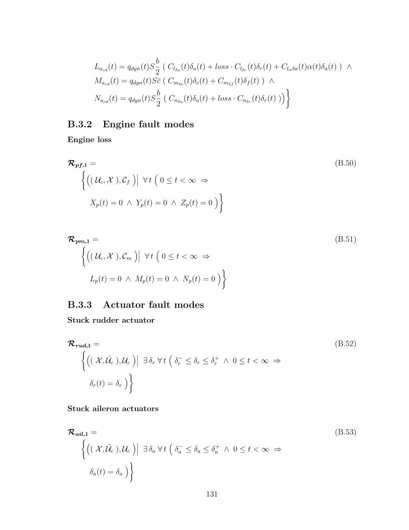
Lacd(t) = qdyn(t)S
b
2( Clδa
(t)δa(t) + loss · Clδr(t)δr(t) + Clαδa(t)α(t)δa(t) ) ∧
Macd(t) = qdyn(t)Sc ( Cmδe
(t)δe(t) + Cmδf(t)δf (t) ) ∧
Nacd(t) = qdyn(t)S
b
2( Cnδa
(t)δa(t) + loss · Cnδr(t)δr(t) )
)}
B.3.2 Engine fault modes
Engine loss
Rpf,1 = (B.50){(( Uc,X ), Cf
)∣∣∣ ∀ t(
0 ≤ t < ∞ ⇒
Xp(t) = 0 ∧ Yp(t) = 0 ∧ Zp(t) = 0)}
Rpm,1 = (B.51){(( Uc,X ), Cm
)∣∣∣ ∀ t(
0 ≤ t < ∞ ⇒
Lp(t) = 0 ∧ Mp(t) = 0 ∧ Np(t) = 0)}
B.3.3 Actuator fault modes
Stuck rudder actuator
Rrud,1 = (B.52){(( X , Uc ),Uc
)∣∣∣ ∃ δr ∀ t(
δ−r ≤ δr ≤ δ+r ∧ 0 ≤ t < ∞ ⇒
δr(t) = δr
)}
Stuck aileron actuators
Rail,1 = (B.53){(( X , Uc ),Uc
)∣∣∣ ∃ δa ∀ t(
δ−a ≤ δa ≤ δ+a ∧ 0 ≤ t < ∞ ⇒
δa(t) = δa
)}
131

Stuck elevator actuators
Relv,1 = (B.54){(( X , Uc ),Uc
)∣∣∣ ∃ δe∀ t(
δ−e ≤ δe ≤ δ+e ∧ 0 ≤ t < ∞ ⇒
δe(t) = δe
)}
Stuck flap actuators
Rflp,1 = (B.55){(( X , Uc ),Uc
)∣∣∣ ∃ δf∀ t(
δ−f ≤ δf ≤ δ+f ∧ 0 ≤ t < ∞ ⇒
δf (t) = δf
)}
B.3.4 Rate gyro fault modes
Bad connection at roll rate gyro output
Rp,1 = (B.56){(X , X
)∣∣∣ ∀ t(
0 ≤ t < ∞ ⇒
p(t) = OR−g ∨ p(t) = OR+
g
)}
Bad connection at pitch rate gyro output
Rq,1 = (B.57){(X , X
)∣∣∣ ∀ t(
0 ≤ t < ∞ ⇒
q(t) = OR−g ∨ q(t) = OR+
g
)}
Bad connection at yaw rate gyro output
Rr,1 = (B.58){(X , X
)∣∣∣ ∀ t(
0 ≤ t < ∞ ⇒
r(t) = OR−g ∨ r(t) = OR+
g
)}
132

B.3.5 Accelerometer fault modes
Bad connection at Ax accelerometer output
RAx,1 = (B.59){(X , X
)∣∣∣ ∀ t(
0 ≤ t < ∞ ⇒
Ax(t) = OR−A ∨ Ax(t) = OR+
A
)}
Bad connection at Ay accelerometer output
RAy,1 = (B.60){(X , X
)∣∣∣ ∀ t(
0 ≤ t < ∞ ⇒
Ay(t) = OR−A ∨ Ay(t) = OR+
A
)}
Bad connection at Az accelerometer output
RAz,1 = (B.61){(X , X
)∣∣∣ ∀ t(
0 ≤ t < ∞ ⇒
Az(t) = OR−A ∨ Az(t) = OR+
A
)}
B.3.6 Air data sensor fault modes
Bad connection at dynamic pressure sensor output
Rqdyn,1 = (B.62){(X , X
)∣∣∣ ∀ t(
0 ≤ t < ∞ ⇒
qdyn(t) = OR−qdyn
∨ qdyn(t) = OR+qdyn
)}
133

Bad connection at static pressure sensor output
Rps,1 = (B.63){(X , X
)∣∣∣ ∀ t(
0 ≤ t < ∞ ⇒
ps(t) = OR−ps
∨ ps(t) = OR+ps
)}
Bad connection at temperature sensor output
RT,1 = (B.64){(X , X
)∣∣∣ ∀ t(
0 ≤ t < ∞ ⇒
T (t) = OR−T ∨ T (t) = OR+
T
)}
B.3.7 Angle of attack sensor fault modes
Bad connection at angle of attack sensor output
Rα,1 = (B.65){(X , X
)∣∣∣ ∀ t(
0 ≤ t < ∞ ⇒
α(t) = OR−α ∨ α(t) = OR+
α
)}
B.3.8 Attitude and heading sensor fault modes
Bad connection at pitch attitude sensor output
Rθ,1 = (B.66){(X , X
)∣∣∣ ∀ t(
0 ≤ t < ∞ ⇒
θ(t) = OR−φ/θ ∨ θ(t) = OR+
φ/θ
)}
134

Bad connection at roll attitude sensor output
Rφ,1 = (B.67){(X , X
)∣∣∣ ∀ t(
0 ≤ t < ∞ ⇒
φ(t) = OR−φ/θ ∨ φ(t) = OR+
φ/θ
)}
Bad connection at heading sensor output
Rψ,1 = (B.68){(X , X
)∣∣∣ ∀ t(
0 ≤ t < ∞ ⇒
ψ(t) = OR−ψ ∨ ψ(t) = OR+
φ
)}
135
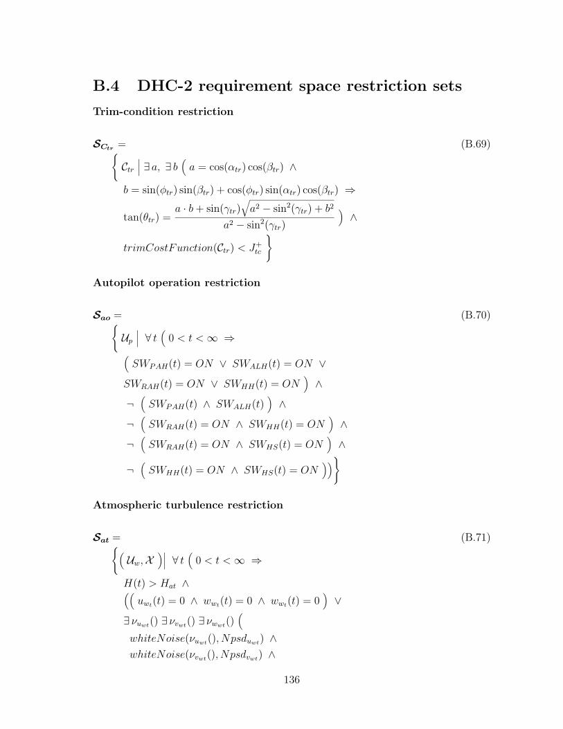
B.4 DHC-2 requirement space restriction sets
Trim-condition restriction
SCtr = (B.69){Ctr
∣∣∣ ∃ a, ∃ b(
a = cos(αtr) cos(βtr) ∧b = sin(φtr) sin(βtr) + cos(φtr) sin(αtr) cos(βtr) ⇒
tan(θtr) =a · b + sin(γtr)
√a2 − sin2(γtr) + b2
a2 − sin2(γtr)
)∧
trimCostFunction(Ctr) < J+tc
}
Autopilot operation restriction
Sao = (B.70){Up
∣∣∣ ∀ t(
0 < t < ∞ ⇒(SWPAH(t) = ON ∨ SWALH(t) = ON ∨
SWRAH(t) = ON ∨ SWHH(t) = ON)
∧¬
(SWPAH(t) ∧ SWALH(t)
)∧
¬(
SWRAH(t) = ON ∧ SWHH(t) = ON)
∧¬
(SWRAH(t) = ON ∧ SWHS(t) = ON
)∧
¬(
SWHH(t) = ON ∧ SWHS(t) = ON))}
Atmospheric turbulence restriction
Sat = (B.71){(Uw,X
)∣∣∣ ∀ t(
0 < t < ∞ ⇒H(t) > Hat ∧((
uwt(t) = 0 ∧ wwt(t) = 0 ∧ wwt(t) = 0)
∨∃ νuwt() ∃ νvwt() ∃ νwwt()
(whiteNoise(νuwt(), Npsduwt) ∧whiteNoise(νvwt(), Npsdvwt) ∧
136

whiteNoise(νwwt(), Npsdwwt) ⇒uwt(t) ' huwt(t, Va(t)) ⊗ νuwt(t) ∧vwt(t) ' hvwt(t, Va(t)) ⊗ νvwt(t) ∧wwt(t) ' hwwt(t, Va(t)) ⊗ νwwt(t)
))∧
uw(t) = 0 ∧ vw(t) = 0 ∧ ww(t) = 0 ∧uwg(t) = 0 ∧ vwg(t) = 0 ∧ wwg(t) = 0
)}(B.72)
137
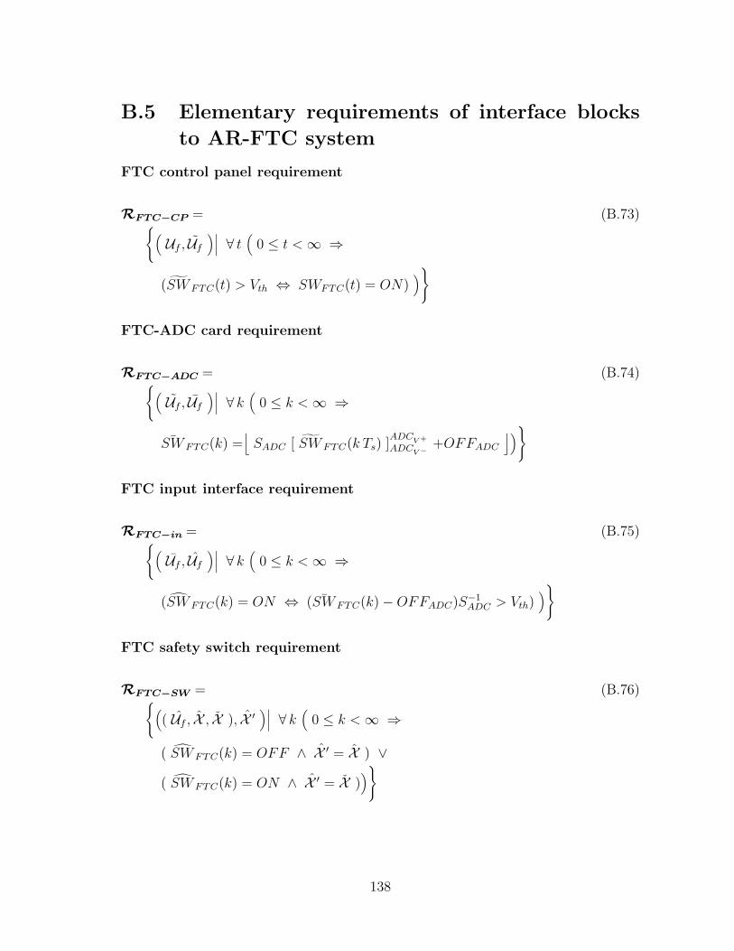
B.5 Elementary requirements of interface blocks
to AR-FTC system
FTC control panel requirement
RFTC−CP = (B.73){(Uf , Uf
)∣∣∣ ∀ t(
0 ≤ t < ∞ ⇒
(SW FTC(t) > Vth ⇔ SWFTC(t) = ON))}
FTC-ADC card requirement
RFTC−ADC = (B.74){(Uf , Uf
)∣∣∣ ∀ k(
0 ≤ k < ∞ ⇒
¯SW FTC(k) =⌊
SADC [ SW FTC(k Ts) ]ADCV +
ADCV − +OFFADC
⌋)}
FTC input interface requirement
RFTC−in = (B.75){(Uf , Uf
)∣∣∣ ∀ k(
0 ≤ k < ∞ ⇒
(SW FTC(k) = ON ⇔ ( ¯SW FTC(k) − OFFADC)S−1ADC > Vth)
)}
FTC safety switch requirement
RFTC−SW = (B.76){(( Uf , X , X ), X ′
)∣∣∣ ∀ k(
0 ≤ k < ∞ ⇒
( SW FTC(k) = OFF ∧ X ′ = X ) ∨( SW FTC(k) = ON ∧ X ′ = X )
)}
138

FTC output interface requirement
RFTC−out = (B.77){(Yf , Yf
)∣∣∣ ∀ k(
0 ≤ k < ∞ ⇒(
Wp(k) >⌊
SDAC
[Vth
]DACV +
DACV −+OFFDAC
⌋⇔ Wp(k) = ON
)∧(
Wq(k) >⌊
SDAC
[Vth
]DACV +
DACV −+OFFDAC
⌋⇔ Wq(k) = ON
)∧(
Wr(k) >⌊
SDAC
[Vth
]DACV +
DACV −+OFFDAC
⌋⇔ Wr(k) = ON
)∧(
Wps(k) >⌊
SDAC
[Vth
]DACV +
DACV −+OFFDAC
⌋⇔ Wps(k) = ON
)∧(
Wqdyn(k) >
⌊SDAC
[Vth
]DACV +
DACV −+OFFDAC
⌋⇔ Wqdyn
(k) = ON)
∧(WT (k) >
⌊SDAC
[Vth
]DACV +
DACV −+OFFDAC
⌋⇔ WT (k) = ON
)∧(
Wφ(k) >⌊
SDAC
[Vth
]DACV +
DACV −+OFFDAC
⌋⇔ Wφ(k) = ON
)∧(
Wθ(k) >⌊
SDAC
[Vth
]DACV +
DACV −+OFFDAC
⌋⇔ Wθ(k) = ON
)∧
(Wψ(k) >
⌊SDAC
[Vth
]DACV +
DACV −+OFFDAC
⌋⇔ Wψ(k) = ON
))}
FTC-DAC card requirement
RFTC−DAC = (B.78){(Yf , Yf
)∣∣∣ ∀ k ∀ t(
0 ≤ k < ∞ ∧ kTs ≤ t < (k + 1)Ts ⇒Wp(t) = (Wp(k) − OFFDAC)S−1
DAC ∧Wq(t) = (Wq(k) − OFFDAC)S−1
DAC ∧Wr(t) = (Wr(k) − OFFDAC)S−1
DAC ∧Wps(t) = (Wps(k) − OFFDAC)S−1
DAC ∧Wqdyn
(t) = (Wqdyn(k) − OFFDAC)S−1
DAC ∧WT (t) = (WT (k) − OFFDAC)S−1
DAC ∧Wφ(t) = (Wφ(k) − OFFDAC)S−1
DAC ∧Wθ(t) = (Wθ(k) − OFFDAC)S−1
DAC ∧Wψ(t) = (Wψ(k) − OFFDAC)S−1
DAC
)}
139

FTC display panel requirement
RFTC−DP = (B.79){(Yf ,Yf
)∣∣∣ ∀ k(
0 ≤ k < ∞ ⇒
Wp(t) = ON ⇔ Wp(t) > Vth ∧Wq(t) = ON ⇔ Wq(t) > Vth ∧Wr(t) = ON ⇔ Wr(t) > Vth ∧Wps(t) = ON ⇔ Wps(t) > Vth ∧Wqdyn
(t) = ON ⇔ Wqdyn(t) > Vth ∧
WT (t) = ON ⇔ WT (t) > Vth ∧Wφ(t) = ON ⇔ Wφ(t) > Vth ∧Wψ(t) = ON ⇔ Wψ(t) > Vth ∧Wθ(t) = ON ⇔ Wθ(t) > Vth
)}
140

Appendix C
Support tables of the specification
This appendix collects all tables supporting the relational specification of appendix
B. The following list briefly describes the role and content of each table.
Table C.1 lists all elementary requirements, of the FTC environment, along with
related domain and image variables, and expanded domain and image spaces.
The table is divided in sub-tables according to the requirements partitioning
performed in appendix B.
Table C.2 lists all requirements obtained by composition of elementary requirements
of the FTC environment.
Table C.3 lists all fault-mode relations.
Table C.4 lists all pre-restriction sets.
Table C.5 lists all equivalent variables and the related equivalence classes that result
from the first expansion over the domain and image spaces of the elementary
specifications.
Table C.6 lists all domain and image variables used within the specification.
141

Table C.7 lists all constants along with their value, type, and description.
Table C.8 lists the quantified variables introduced in the relational specifications
along with their type and description.
Table C.9 defines all auxiliary terms. The table is divided in sub-tables to distin-
guish between auxiliary terms, functions, and predicates.
Table C.10 defines all types used within the specification.
142

Table C.1: Elementary requirements
ID Name Domain variables Image variables Domain and imagespaces
Extended domainand image spaces
AFCS performance requirementsRALH altitude hold SWALH(), φ(), Va(),
uwt(), vwt(), wwt(),uwg(), vwg(), wwg()
An(), H() Uw+Upa +X × X Uw+Upa+X+Ctr×X
RHH heading hold SWHH(),uwt(), vwt(), wwt(),uwg(), vwg(), wwg()
φ(), ψ() Uw+Upa × X Uw+Upa+X+Ctr×X
RHS heading select SWHS(), ψr(),uwt(), vwt(), wwt(),uwg(), vwg(), wwg()
φ(), ψ(), p() Uw+Upa × X Uw+Upa+X+Ctr×X
RPAH pitch attitudehold
SWPAH(), θr(), φ(),uwt(), vwt(), wwt(),uwg(), vwg(), wwg()
θ() Uw+Upa +X × X Uw+Upa+X+Ctr×X
RRAH roll attitudehold
SWRAH(), φr(),uwt(), vwt(), wwt(),uwg(), vwg(), wwg()
φ() Uw+Upa +X × X Uw+Upa+X+Ctr×X
DHC-2 dynamics requirementsRFeq force equations
of aircraft dy-namics
Xasd(), Xacd
(),Xp(), Xgr(), Xw(),Yasd
(), Yacd(),
Yp(), Ygr(), Yw(),Zasd
(), Zacd(),
Zp(), Zgr(), Zw(),p(), q(), r()
Va(), α(), β() Cf+X × X Cf+X × X
RKeq kinematicequations
p(), q(), r() ψ(), θ(), φ() X × X Uc+Uw+Upm+X ×X
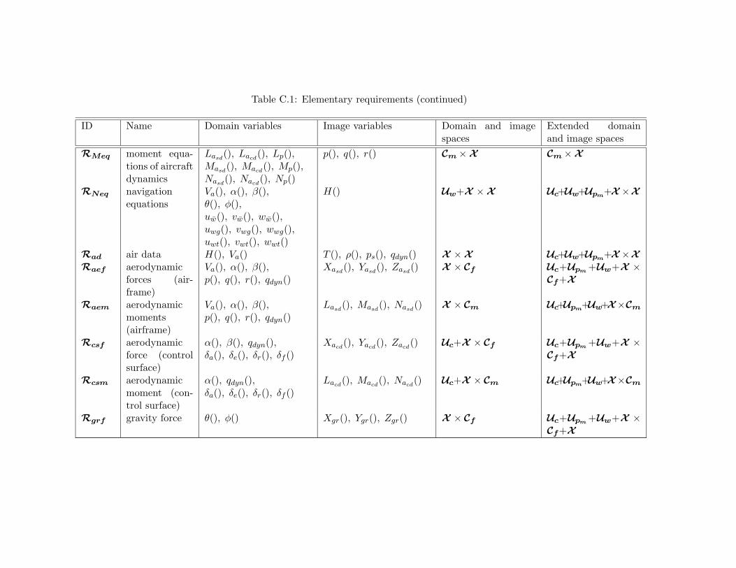
Table C.1: Elementary requirements (continued)
ID Name Domain variables Image variables Domain and imagespaces
Extended domainand image spaces
RMeq moment equa-tions of aircraftdynamics
Lasd(), Lacd
(), Lp(),Masd
(), Macd(), Mp(),
Nasd(), Nacd
(), Np()
p(), q(), r() Cm × X Cm × X
RNeq navigationequations
Va(), α(), β(),θ(), φ(),uw(), vw(), ww(),uwg(), vwg(), wwg(),uwt(), vwt(), wwt()
H() Uw+X × X Uc+Uw+Upm+X ×X
Rad air data H(), Va() T (), ρ(), ps(), qdyn() X × X Uc+Uw+Upm+X ×XRaef aerodynamic
forces (air-frame)
Va(), α(), β(),p(), q(), r(), qdyn()
Xasd(), Yasd
(), Zasd() X × Cf Uc+Upm +Uw+X ×
Cf+X
Raem aerodynamicmoments(airframe)
Va(), α(), β(),p(), q(), r(), qdyn()
Lasd(), Masd
(), Nasd() X × Cm Uc+Upm+Uw+X×Cm
Rcsf aerodynamicforce (controlsurface)
α(), β(), qdyn(),δa(), δe(), δr(), δf ()
Xacd(), Yacd
(), Zacd() Uc+X × Cf Uc+Upm +Uw+X ×
Cf+X
Rcsm aerodynamicmoment (con-trol surface)
α(), qdyn(),δa(), δe(), δr(), δf ()
Lacd(), Macd
(), Nacd() Uc+X × Cm Uc+Upm+Uw+X×Cm
Rgrf gravity force θ(), φ() Xgr(), Ygr(), Zgr() X × Cf Uc+Upm +Uw+X ×Cf+X

Table C.1: Elementary requirements (continued)
ID Name Domain variables Image variables Domain and imagespaces
Extended domainand image spaces
Rka kinematic ac-celeration (atcrew station)
Va(), α(), β(),uw(), vw(), ww(),uwt(), vwt(), wwt(),uwg(), vwg(), wwg(),p(), q(), r()
Ax(), Ay(), Az() Uw+X × X Uc+Uw+Upm+X ×X
Rpf propulsiveforce
qdyn(), ρ(), Va(), α(),n(), pz()
Xp(), Yp(), Zp() Upm +X × Cf Uc+Upm +Uw+X ×Cf+X
Rpm propulsive mo-ment
qdyn(), ρ(), Va(), α(),n(), pz()
Lp(), Mp(), Np() Upm +X × Cm Uc+Upm+Uw+X×Cm
Rwf wind force uw(), vw(), ww(),uwt(), vwt(), wwt(),uwg(), vwg(), wwg(),p(), q(), r()
Xw(), Yw(), Zw() X+Uw × Cf Uc+Upm +Uw+X ×Cf+X
DHC-2 AFCS hardware requirements
RADC A/D interface p(), q(), r(),Ax(), Ay(), Az(),ps(), qdyn(), α(),ψ(), θ(), φ(),ψr(), φr(), θr(),SWPAH(), SWALH(),SWRAH(),SWHH(), SWHS()
p(), q(), r(),Ax(), Ay(), Az(),ps(), qdyn(), α(),ψ(), θ(), φ(),ψr(), φr(), θr(),¯SWPAH(), ¯SWALH(),¯SWRAH(),¯SWHH(), ¯SWHS()
X+Upa × X+Upa X+Upa × X+Upa
RAx Ax accelerome-ter
Ax(), θ() Ax() X × X Upa +X × Upa +X
RAy Ay accelerome-ter
Ay(), θ(), φ() Ay() X × X Upa +X × Upa +X
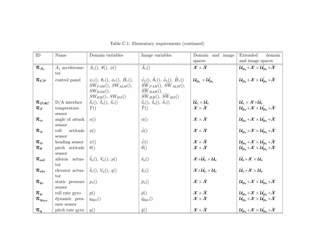
Table C.1: Elementary requirements (continued)
ID Name Domain variables Image variables Domain and imagespaces
Extended domainand image spaces
RAz Az accelerome-ter
Az(), θ(), φ() Az() X × X Upa +X × Upa +X
RCP control panel ψr(), θr(), φr(), Hr(),SWPAH(), SWALH(),SWRAH(),SWHH(), SWHS()
ψr(), θr(), φr(),˜Hr()
SWPAH(), SWALH(),SWRAH(),SWHH(), SWHS()
Upa × Upa Upa +X × Upa +X
RDAC D/A interface δe(), δa(), δr() δe(), δa(), δr() Uc × Uc Uc × X+Uc
RT temperaturesensor
T () T () X × X Upa +X × Upa +X
Rα angle of attacksensor
α() α() X × X Upa +X × Upa +X
Rφ roll attitudesensor
φ() φ() X × X Upa +X × Upa +X
Rψ heading sensor ψ() ψ() X × X Upa +X × Upa +XRθ pitch attitude
sensorθ() θ() X × X Upa +X × Upa +X
Rail aileron actua-tor
δa(), Va(), p() δa() X+Uc × Uc Uc+X × Uc
Relv elevator actua-tor
δe(), Va(), q() δe() X+Uc × Uc Uc+X × Uc
Rps static pressuresensor
ps() ps() X × X Upa +X × Upa +X
Rp roll rate gyro p() p() X × X Upa +X × Upa +XRqdyn dynamic pres-
sure sensorqdyn() qdyn() X × X Upa +X × Upa +X
Rq pitch rate gyro q() q() X × X Upa +X × Upa +X

Table C.1: Elementary requirements (continued)
ID Name Domain variables Image variables Domain and imagespaces
Extended domainand image spaces
Rrud rudder actua-tor
δr(), Va(), r() δr() X+Uc × Uc Uc+X × Uc
Rr yaw rate gyro r() r() X × X Upa +X × Upa +XDHC-2 AFCS software requirements
Rin Software inputinterface
p(), q(), r(),Ax(), Ay(), Az(),ps(), qdyn(), α(),ψ(), θ(), φ(),ψr(), φr(), θr(),¯SWPAH(), ¯SWALH(),¯SWRAH(),¯SWHH(), ¯SWHS()
p(), q(), r(),Ax(), Ay(), Az(),ps(), qdyn(), α(),ψ(), θ(), φ(),ψr(), φr(), θr(),SWPAH(), SWALH(),SWRAH(),SWHH(), SWHS()
X+Upa × X+Upa X+Upa × X+Upa
Rout Software out-put interface
δe(), δa(), δr() δe(), δa(), δr() Uc × Uc Uc × Uc
RALH
altitude holdautopilot
Va(), q(), r(), φ(), θ(),H(), Hr(), SWALH()
δe() Upa +X × Uc Upa +X × Uc
RHH
heading holdautopilot
Va(), r(), φ(), ψ(),SWHH()
δa(), δr() Upa +X × Uc Upa +X × Uc
RHS
heading selectautopilot
Va(), r(), φ(), ψ(),ψr(), SWHS()
δa(), δr() Upa +X × Uc Upa +X × Uc
RPAH
pitch attitudehold autopilot
Va(), q(), r(), φ(), θ(),θr(), SWPAH()
δe() Upa +X × Uc Upa +X × Uc
RRAH
roll attitudehold autopilot
Va(), r(), φ(),φr(), SWRAH()
δa(), δr() Upa +X × Uc Upa +X × Uc
FTC interface requirements (the FTC acronym has been omitted from the identifier for the sake of space)
R−ADC FTC A/D card SWFTC() ¯SWFTC() Uf × Uf not used

Table C.1: Elementary requirements (continued)
ID Name Domain variables Image variables Domain and imagespaces
Extended domainand image spaces
R−CP FTC controlpanel
SWFTC() SWFTC() Uf × Uf not used
R−DAC FTC D/A card Wp(), Wq, Wr,Wps , Wqdyn
, WT ,Wφ, Wψ, Wθ
Wp(), Wq, Wr,Wps , Wqdyn
, WT ,
Wφ, Wψ, Wθ
Yf × Yf not used
R−DP FTC displaypanel
Wp(), Wq, Wr,Wps , Wqdyn
, WT ,
Wφ, Wψ, Wθ
Wp(), Wq, Wr,Wps , Wqdyn
, WT ,Wφ, Wψ, Wθ
Yf × Yf not used
R−in FTC input in-terface
¯SWFTC() SWFTC() Uf × Uf not used
R−out FTC outputinterface
Wp(), Wq, Wr,Wps , Wqdyn
, WT ,
Wφ, Wψ, Wθ
Wp(), Wq, Wr,Wps , Wqdyn
, WT ,Wφ, Wψ, Wθ
Yf × Yf not used

Table C.2: Composed requirements
ID Description Extended domain and image spaces
AFCS performance specificationRPS performance specification Ctr+Upa +X+Uw × X
DHC-2 detail specification
RACT control surface actuators Uc+X × Uc
RAFCS automatic flight control system Upa +X × Uc
RCin computer input Upa +X × Upa +XRDHC2 DHC-2 airplane dynamics Uc+Uw+Upm +X × XRFCC flight control computer Upa +X × Uc+XRFCL flight control laws Upa +X × Uc
RFCSw flight control software Upa +X × Uc
RSp primary sensors Upa +X × Upa +XRSs secondary sensors Upa +X × Upa +XRf forces exerted upon the airplane Uc+Upm +Uw+X × Cf+XRm moments exerted upon the airplane Uc+Upm +Uw+X × Cm

Table C.3: Fault modes
ID Description Domain and image spaces and variablesRcsf,1 partial loss of rudder surface same as Rcsf
Rcsm,1 partial loss of rudder surface same as Rcsm
Rpf,1 engine loss same as Rpf
Rpm,1 engine loss same as Rpm
RAx,1 Bad connection at Ax accelerometer output same as RAx
RAy,1 Bad connection at Ay accelerometer output same as RAy
RAz,1 Bad connection at Az accelerometer output same as RAz
RT,1 Bad connection at temperature sensor output same as RT
Rα,1 Bad connection at angle of attack sensor output same as Rα
Rφ,1 Bad connection at roll attitude sensor output same as Rφ
Rψ,1 Bad connection at heading sensor output same as Rψ
Rθ,1 Bad connection at pitch attitude sensor output same as Rθ
Rail,1 Stuck aileron actuator same as Rail
Relv,1 Stuck elevator actuator same as Relv
Rps,1 Bad connection at static pressure sensor output same as Rps
Rp,1 Bad connection at roll rate gyro output same as Rp
Rqdyn Bad connection at dynamic pressure sensor output same as Rqdyn
Rq,1 Bad connection at pitch rate gyro output same as Rq
Rrud,1 Stuck rudder actuator same as Rrud
Rr,1 Bad connection at yaw rate gyro output same as Rr

Table C.4: Restriction sets
ID Description Variables Space Extended spaceSCtr Trim-condition Vatr, αtr, βtr, ptr, qtr, rtr, ψtr, θtr, φtr, Htr,
γtr, δatr, δetr, δrtr, δftr, ntr, pztr
Ctr Ctr+Upa +X+Uw
Sao Autopilot opera-tion
SWPAH(), SWALH(),SWRAH(), SWHH(), SWHS()
Upa Ctr+Upa +X+Uw
Sat Atmospheric tur-bulence
uw(), vw(), ww(), uwt(), vwt(), wwt(),uwg(), vwg(), wwg(), H()
Uw+X Ctr+Upa +X+Uw

Table C.5: Spaces used within the requirements specification
Spaceidentifier
Spaceelementidentifier
Space element variables
Spaces introduced for the requirements specification of the FTC environmentCf Cf Xasd
(), Yasd(), Zasd
(), Xgr(), Ygr(), Zgr(), Xw(), Yw(), Zw(), Xacd(), Yacd
(), Zacd(), Xp(), Yp(), Zp()
Cm Cm Lasd(), Masd
(), Nasd(), Lacd
(), Macd(), Nacd
(), Lp(), Mp(), Np()Ctr Ctr Vatr, αtr, βtr, ptr, qtr, rtr, ψtr, θtr, φtr, Htr, γtr, δatr, δetr, δrtr, δftr, ntr, pztr
Uc Uc δa(), δe(), δr()Upa Upa SWPAH(), SWALH(), SWRAH(), SWHH(), SWHS(), φr(), ψr(), θr()Upm Upm δf (), n(), pz()Uw Uw uw(), vw(), ww(), uwt(), vwt(), wwt(), uwg(), vwg(), wwg()X X Va(), α(), β(), p(), q(), r(), ψ(), θ(), φ(), H(), Ax(), Ay(), Az(), ps(), qdyn(), T (), ρ()Uc Uc δa(), δe(), δr()Upa Upa
¯SWPAH(), ¯SWALH(), ¯SWRAH(), ¯SWHH(), ¯SWHS(), φr(), ψr(), θr()X X α(), β(), p(), q(), r(), ψ(), φ(), θ(), Ax(), Ay(), Az(), ps(), qdyn(), T ()Uc Uc δa(), δe(), δr()Upa Upa SWPAH(), SWALH(), SWRAH(), SWHH(), SWHS(), φr(), ψr(), θr()X X Va(), α(), β(), p(), q(), r(), ψ(), θ(), φ(), H(), Ax(), Ay(), Az(), ps(), qdyn(), T ()Uc Uc δa(), δe(), δr()Upa Upa SWPAH(), SWALH(), SWRAH(), SWHH(), SWHS(), φr(), ψr(), θr()X X α(), β(), p(), q(), r(), ψ(), θ(), φ(), Ax(), Ay(), Az(), ps(), qdyn(), T ()
Spaces introduced for the requirements specification of the FTC systemUf Uf SWFTC()Yf Yf Wp(), Wq(), Wr(), Wps(), Wqdyn
(), WT (), Wφ(), Wθ(), Wψ()Uf Uf
¯SWFTC()Yf Yf Wp(), Wq(), Wr(), Wps(), Wqdyn
(), WT (), Wφ(), Wθ(), Wψ()Uf Uf
ˆSWFTC()Yf Yf Wp(), Wq(), Wr(), Wps(), Wqdyn
(), WT (), Wφ(), Wθ(), Wψ()

Table C.5: Spaces used within the requirements specification (continued)
Spaceidentifier
Spaceelementidentifier
Space element variables
Uf Uf˜SWFTC()
Yf Yf Wp(), Wq(), Wr(), Wps(), Wqdyn(), WT (), Wφ(), Wθ(), Wψ()

Table C.6: Domain and image variables
ID Type Description
Actual-quantity variablesAx() time-T → acceleration-T component along XB-axis of kinematic acceleration at crew stationAy() time-T → acceleration-T component along YB-axis of kinematic acceleration at crew stationAz() time-T → acceleration-T component along ZB-axis of kinematic acceleration at crew stationH() time-T → altitude-T height above sea levelLp() time-T → moment-T propulsive moment about XB-axisLacd
() time-T → moment-T control-surface-exerted aerodynamic moment about XB-axisLasd
() time-T → moment-T airframe-exerted aerodynamic moment about XB-axisMp() time-T → moment-T propulsive moment about YB-axisMacd
() time-T → moment-T control-surface-exerted aerodynamic moment about YB-axisMasd
() time-T → moment-T airframe-exerted aerodynamic moment about YB-axisNp() time-T → moment-T propulsive moment about ZB-axisNacd
() time-T → moment-T control-surface-exerted aerodynamic moment about ZB-axisNasd
() time-T → moment-T airframe-exerted aerodynamic moment about ZB-axisSWALH() time-T → switch-T ALH on/off switchSWHH() time-T → switch-T HH on/off switchSWHS() time-T → switch-T HS on/off switchSWPAH() time-T → switch-T PAH on/off switchSWRAH() time-T → switch-T RAH on/off switchT () time-T → temperature-T air temperatureVa() time-T → airspeed-T airspeedXp() time-T → force-T propulsive force along XB-axisXw() time-T → force-T wind force along XB-axisXacd
() time-T → force-T control-surface-exerted aerodynamic force along XB-axisXasd
() time-T → force-T airframe-exerted aerodynamic force along XB-axisXgr() time-T → force-T gravity force along XB-axisYp() time-T → force-T propulsive force along YB-axisYw() time-T → force-T wind force along YB-axis

Table C.6: Domain and image variables (continued)
ID Type DescriptionYacd
() time-T → force-T control-surface-exerted aerodynamic force along YB-axisYasd
() time-T → force-T airframe-exerted aerodynamic force along YB-axisYgr() time-T → force-T gravity force along YB-axisZp() time-T → force-T propulsive force along ZB-axisZw() time-T → force-T wind force along ZB-axisZacd
() time-T → force-T control-surface-exerted aerodynamic force along ZB-axisZasd
() time-T → force-T airframe-exerted aerodynamic force along ZB-axisZgr() time-T → force-T gravity force along ZB-axisα() time-T → AOT-T angle of attackβ() time-T → angle-T sideslip angleδa() time-T → aileronDeflection-T aileron deflection (δa = δaright
− δaleft)
δe() time-T → elevatorDeflection-T elevator deflectionδf () time-T → flapDeflection-T flap deflectionδr() time-T → rudderDeflection-T rudder deflectionφ() time-T → angle-T roll angleφr() time-T → bankReference-T reference roll angleψ() time-T → angle-T heading angleψr() time-T → headingReference-T reference heading angleρ() time-T → density-T air densityθ() time-T → angle-T pitch angleθr() time-T → pitchReference-T reference pitch anglen() time-T → engineSpeed-T engine speedp() time-T → angularVelocity-T roll angular rateps() time-T → pressure-T static pressurepz() time-T → pressure-T engine manifold pressureq() time-T → angularVelocity-T pitch angular rateqdyn() time-T → pressure-T dynamic pressurer() time-T → angularVelocity-T yaw angular rate

Table C.6: Domain and image variables (continued)
ID Type Descriptionuw() time-T → velocity-T mean wind velocity component along XB-axisuwg() time-T → velocity-T wind-gust velocity component along XB-axisuwt() time-T → velocity-T wind-turbulence velocity component along XB-axisvw() time-T → velocity-T mean wind velocity component along YB-axisvwg() time-T → velocity-T wind-gust velocity component along YB-axisvwt() time-T → velocity-T wind-turbulence velocity component along YB-axisww() time-T → velocity-T mean wind velocity component along ZB-axiswwg() time-T → velocity-T wind-gust velocity component along ZB-axiswwt() time-T → velocity-T wind-turbulence velocity component along ZB-axis
Software-quantity variables
Ax() natural-T → ADCoutput-T ADC software representation of Ax()Ay() natural-T → ADCoutput-T ADC software representation of Ay()Az() natural-T → ADCoutput-T ADC software representation of Az()¯SWALH() natural-T → ADCoutput-T ADC software representation of SWALH()¯SWHH() natural-T → ADCoutput-T ADC software representation of SWHH()¯SWHS() natural-T → ADCoutput-T ADC software representation of SWHS()¯SWPAH() natural-T → ADCoutput-T ADC software representation of SWPAH()¯SWRAH() natural-T → ADCoutput-T ADC software representation of SWRAH()
T () natural-T → ADCoutput-T ADC software representation of T ()α() natural-T → ADCoutput-T ADC software representation of α()δa() natural-T → DACinput-T DAC software representation of δa()δe() natural-T → DACinput-T DAC software representation of δe()δr() natural-T → DACinput-T DAC software representation of δr()φ() natural-T → ADCoutput-T ADC software representation of φ()φr() natural-T → ADCoutput-T ADC software representation of phir()ψ() natural-T → ADCoutput-T ADC software representation of ψ()ψr() natural-T → ADCoutput-T ADC software representation of ψr()

Table C.6: Domain and image variables (continued)
ID Type Description
θ() natural-T → ADCoutput-T ADC software representation of θ()θr() natural-T → ADCoutput-T ADC software representation of θr()p() natural-T → ADCoutput-T ADC software representation of p()ps() natural-T → ADCoutput-T ADC software representation of ps()q() natural-T → ADCoutput-T ADC software representation of q()qdyn() natural-T → ADCoutput-T ADC software representation of qdyn()r() natural-T → ADCoutput-T ADC software representation of r()Ax() natural-T → acceleration-T software variable representing Ax()Ay() natural-T → acceleration-T software variable representing Ay()Az() natural-T → acceleration-T software variable representing Az()H() natural-T → altitude-T software variable representing H()SWALH() natural-T → switch-T software variable representing SWALH()SWHH() natural-T → switch-T software variable representing SWHH()SWHS() natural-T → switch-T software variable representing SWHS()SWPAH() natural-T → switch-T software variable representing SWPAH()SWRAH() natural-T → switch-T software variable representing SWRAH()Va() natural-T → airspeed-T software variable representing Va()α() natural-T → angle-T software variable representing α()δa() natural-T → aileronDeflection-T software variable representing δa()δe() natural-T → elevatorDeflection-T software variable representing δe()δr() natural-T → rudderDeflection-T software variable representing δr()φ() natural-T → angle-T software variable representing φ()φr() natural-T → bankReference-T software variable representing φr()ψ() natural-T → angle-T software variable representing ψ()ψr() natural-T → headingReference-T software variable representing ψr()θ() natural-T → angle-T software variable representing θ()p() natural-T → angularVelocity-T software variable representing p()

Table C.6: Domain and image variables (continued)
ID Type Descriptionps() natural-T → pressure-T software variable representing ps()q() natural-T → angularVelocity-T software variable representing q()qdyn() natural-T → pressure-T software variable representing qdyn()r() natural-T → angularVelocity-T software variable representing r()
Electrical-quantity variables
Ax() time-T → accelerometerOutput-T output of accelerometer along XB-axisAy() time-T → accelerometerOutput-T output of accelerometer along YB-axisAz() time-T → accelerometerOutput-T output of accelerometer along ZB-axisSWALH() time-T → CPOutput-T output of ALH control switchSWHH() time-T → CPOutput-T output of HH control switchSWHS() time-T → CPOutput-T output of HS control switchSWPAH() time-T → CPOutput-T output of PAH control switchSWRAH() time-T → CPOutput-T output of RAH control switchT () time-T → TSensorOutput-T output of temperature sensorα() time-T → AOTSensorOutput-T output of angle of attack sensorδa() time-T → PCUInput-T input to aileron PCU (+0.5α() to right aileron PCU and (−0.5α()
to left aileron PCUδe() time-T → PCUInput-T input to elevator PCUδf () time-T → PCUInput-T input to flap PCUδr() time-T → PCUInput-T input to rudder PCUφ() time-T → attitudeSensorOuput-T output of roll attitude sensorφr() time-T → CPOutput-T output of reference roll control knobψ() time-T → headingSensorOutput-T output of heading sensorψr() time-T → CPOutput-T output of reference heading control knobθ() time-T → attitudeSensorOuput-T output of pitch attitude sensorθr() time-T → attitudeSensorOuput-T output of reference pitch control knobp() time-T → gyroOutput-T output of roll rate gyro

Table C.6: Domain and image variables (continued)
ID Type Descriptionps() time-T → psSensorOutput-T output of static pressure sensorq() time-T → gyroOutput-T output of pitch rate gyroqdyn() time-T → qdynSensorOutput-T output of dynamic pressure sensorr() time-T → gyroOutput-T output of yaw rate gyro
Actual-quantity variables (FTC system)SWFTC() time-T → switch-T FTC on/off switchWT () time-T → warningLight-T temperature sensor warning lightWφ() time-T → warningLight-T roll attitude sensor warning lightWψ() time-T → warningLight-T heading sensor warning lightWθ() time-T → warningLight-T pitch attitude sensor warning lightWp() time-T → warningLight-T roll rate gyro warning lightWq() time-T → warningLight-T pitch rate gyro warning lightWr() time-T → warningLight-T yaw rate gyro warning lightWps() time-T → warningLight-T static pressure sensor warning lightWqdyn
() time-T → warningLight-T dynamic pressure sensor warning lightSoftware-quantity variables (FTC system)
¯SWFTC() natural-T → DACinput-T DAC software representation of SWFTC()WT () natural-T → DACinput-T DAC software representation of T ()Wφ() natural-T → DACinput-T DAC software representation of φ()Wψ() natural-T → DACinput-T DAC software representation of ψ()Wθ() natural-T → DACinput-T DAC software representation of θ()Wp() natural-T → DACinput-T DAC software representation of p()Wq() natural-T → DACinput-T DAC software representation of q()Wr() natural-T → DACinput-T DAC software representation of r()Wps() natural-T → DACinput-T DAC software representation of ps()Wqdyn
() natural-T → DACinput-T DAC software representation of qdyn()SWFTC() natural-T → switch-T software variable representing SWFTC()

Table C.6: Domain and image variables (continued)
ID Type Description
WT () natural-T → warningLight-T software variable representing WT ()Wφ() natural-T → warningLight-T software variable representing Wφ()Wψ() natural-T → warningLight-T software variable representing Wψ()Wθ() natural-T → warningLight-T software variable representing Wθ()Wp() natural-T → warningLight-T software variable representing Wp()Wq() natural-T → warningLight-T software variable representing Wq()Wr() natural-T → warningLight-T software variable representing Wr()Wps() natural-T → warningLight-T software variable representing Wps()Wqdyn
() natural-T → warningLight-T software variable representing Wqdyn()
Electrical-quantity variables (FTC system)
SWFTC() time-T → CPOutput-T output of FTC control switchWp() time-T → warningLightInput-T input to roll rate gyro warning lightWq() time-T → warningLightInput-T input to pitch rate gyro warning lightWr() time-T → warningLightInput-T input to yaw rate gyro warning lightWps() time-T → warningLightInput-T input to static pressure sensor warning lightWqdyn
() time-T → warningLightInput-T input to dynamic pressure sensor warning lightWT () time-T → warningLightInput-T input to temperature sensor warning lightWφ() time-T → warningLightInput-T input to roll attitude sensor warning lightWθ() time-T → warningLightInput-T input to pitch attitude sensor warning lightWψ() time-T → warningLightInput-T input to heading sensor warning light
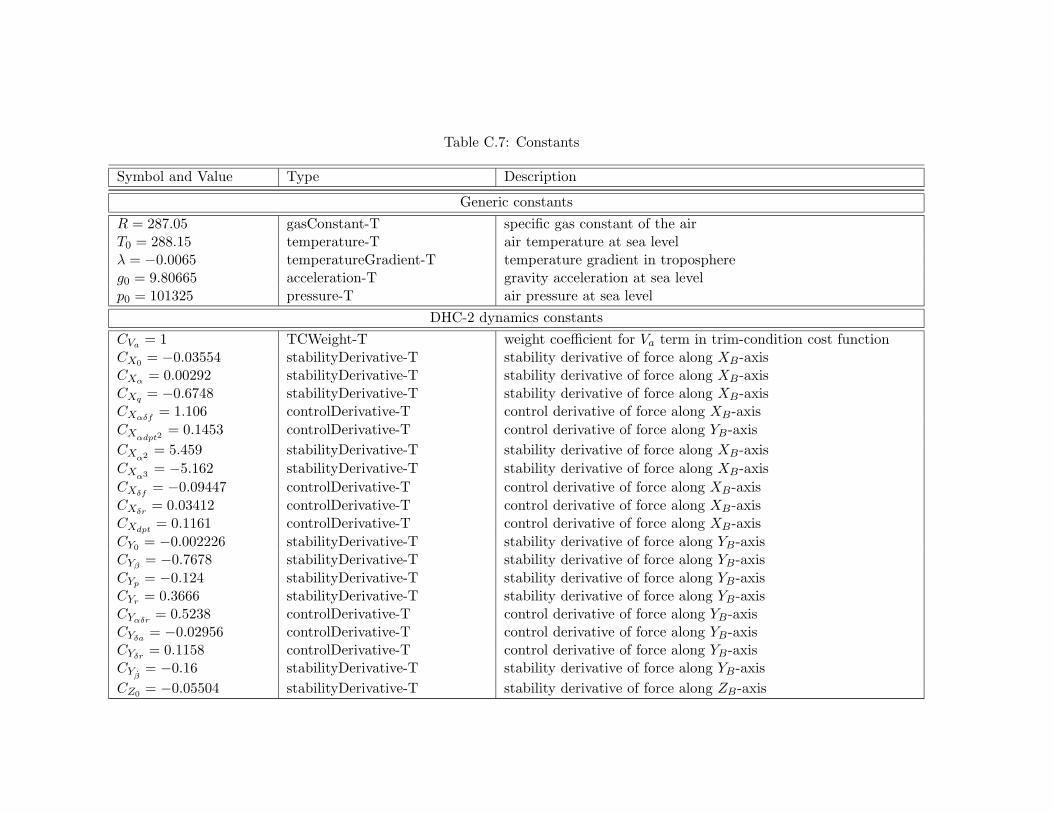
Table C.7: Constants
Symbol and Value Type Description
Generic constantsR = 287.05 gasConstant-T specific gas constant of the airT0 = 288.15 temperature-T air temperature at sea levelλ = −0.0065 temperatureGradient-T temperature gradient in troposphereg0 = 9.80665 acceleration-T gravity acceleration at sea levelp0 = 101325 pressure-T air pressure at sea level
DHC-2 dynamics constantsCVa = 1 TCWeight-T weight coefficient for Va term in trim-condition cost functionCX0 = −0.03554 stabilityDerivative-T stability derivative of force along XB-axisCXα = 0.00292 stabilityDerivative-T stability derivative of force along XB-axisCXq = −0.6748 stabilityDerivative-T stability derivative of force along XB-axisCXαδf
= 1.106 controlDerivative-T control derivative of force along XB-axisCXαdpt2
= 0.1453 controlDerivative-T control derivative of force along YB-axisCXα2 = 5.459 stabilityDerivative-T stability derivative of force along XB-axisCXα3 = −5.162 stabilityDerivative-T stability derivative of force along XB-axisCXδf
= −0.09447 controlDerivative-T control derivative of force along XB-axisCXδr
= 0.03412 controlDerivative-T control derivative of force along XB-axisCXdpt
= 0.1161 controlDerivative-T control derivative of force along XB-axisCY0 = −0.002226 stabilityDerivative-T stability derivative of force along YB-axisCYβ
= −0.7678 stabilityDerivative-T stability derivative of force along YB-axisCYp = −0.124 stabilityDerivative-T stability derivative of force along YB-axisCYr = 0.3666 stabilityDerivative-T stability derivative of force along YB-axisCYαδr
= 0.5238 controlDerivative-T control derivative of force along YB-axisCYδa
= −0.02956 controlDerivative-T control derivative of force along YB-axisCYδr
= 0.1158 controlDerivative-T control derivative of force along YB-axisCYβ
= −0.16 stabilityDerivative-T stability derivative of force along YB-axisCZ0 = −0.05504 stabilityDerivative-T stability derivative of force along ZB-axis

Table C.7: Constants (continued)
Symbol and Value Type DescriptionCZα = −5.578 stabilityDerivative-T stability derivative of force along ZB-axisCZq = −2.998 stabilityDerivative-T stability derivative of force along ZB-axisCZαδf
= −1.261 controlDerivative-T control derivative of force along ZB-axisCZα3 = 3.442 stabilityDerivative-T stability derivative of force along ZB-axisCZβ2δe
= −15.93 controlDerivative-T control derivative of force along ZB-axisCZδe
= −0.398 controlDerivative-T control derivative of force along ZB-axisCZδf
= −1.377 controlDerivative-T control derivative of force along ZB-axisCZdpt
= −0.1563 controlDerivative-T control derivative of force along ZB-axisCαβ = 2 TCWeight-T weight coefficient for α and β terms in trim-condition cost functionCl0 = 0.000591 stabilityDerivative-T stability derivative of moment about XB-axisClβ = −0.0618 stabilityDerivative-T stability derivative of moment about XB-axisClp = −0.5045 stabilityDerivative-T stability derivative of moment about XB-axisClr = 0.1695 stabilityDerivative-T stability derivative of moment about XB-axisClαδa
= −0.08269 controlDerivative-T control derivative of moment about XB-axisClα2dpt
= −0.01406 controlDerivative-T control derivative of moment about XB-axisClδa
= −0.09917 controlDerivative-T control derivative of moment about XB-axisClδr
= 0.006934 controlDerivative-T control derivative of moment about XB-axisCm0 = 0.09448 stabilityDerivative-T stability derivative of moment about YB-axisCm∗
α= −0.6028 stabilityDerivative-T nominal value of stability derivative of moment about YB-axis
Cm+α
= −0.428 stabilityDerivative-T maximum value of stability derivative of moment about YB-axisCm−
α= −1.8 stabilityDerivative-T minimum value of stability derivative of moment about YB-axis
Cmq = −15.56 stabilityDerivative-T stability derivative of moment about YB-axisCmr = −0.3118 stabilityDerivative-T stability derivative of moment about YB-axisCmα2 = −2.14 stabilityDerivative-T stability derivative of moment about YB-axisCmβ2 = 0.6921 stabilityDerivative-T stability derivative of moment about YB-axisCmδe
= −1.921 controlDerivative-T control derivative of moment about YB-axisCmδf
= 0.4072 controlDerivative-T control derivative of moment about YB-axisCmdpt
= −0.07895 controlDerivative-T control derivative of moment about YB-axis
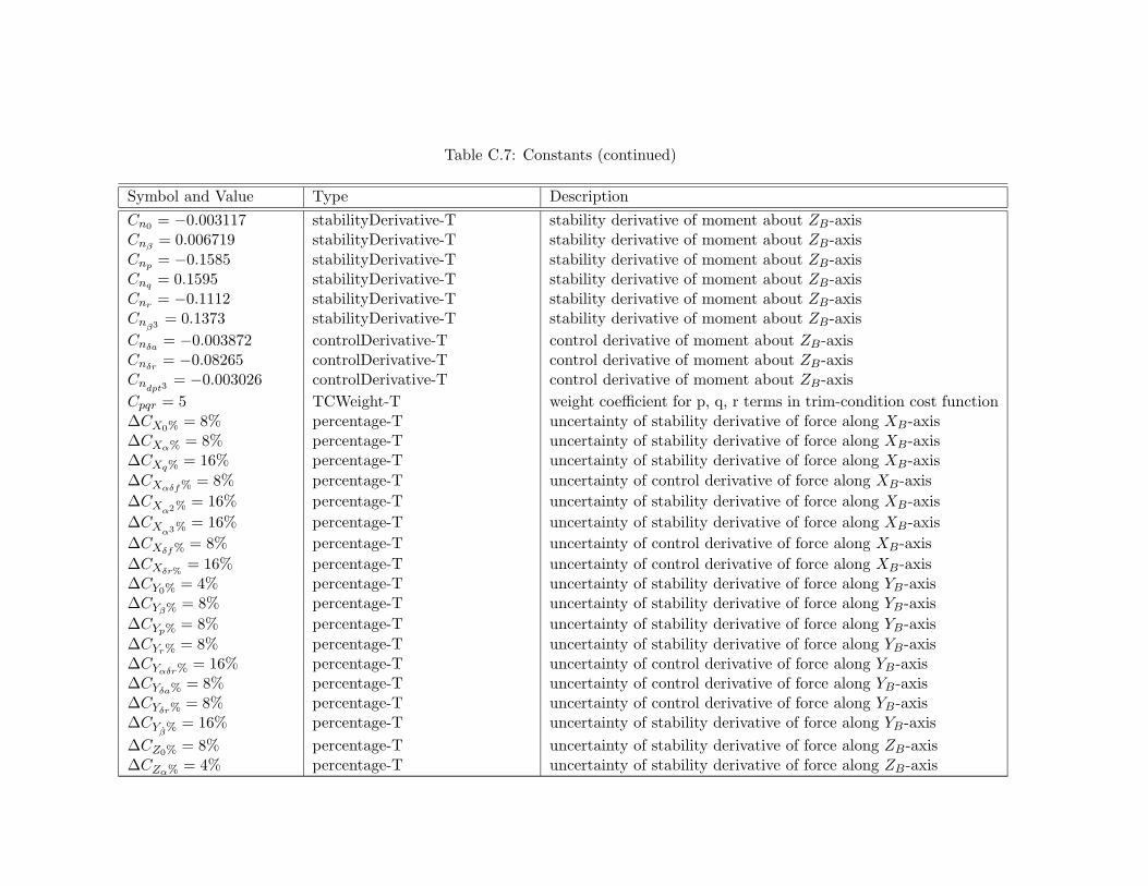
Table C.7: Constants (continued)
Symbol and Value Type DescriptionCn0 = −0.003117 stabilityDerivative-T stability derivative of moment about ZB-axisCnβ
= 0.006719 stabilityDerivative-T stability derivative of moment about ZB-axisCnp = −0.1585 stabilityDerivative-T stability derivative of moment about ZB-axisCnq = 0.1595 stabilityDerivative-T stability derivative of moment about ZB-axisCnr = −0.1112 stabilityDerivative-T stability derivative of moment about ZB-axisCnβ3 = 0.1373 stabilityDerivative-T stability derivative of moment about ZB-axisCnδa
= −0.003872 controlDerivative-T control derivative of moment about ZB-axisCnδr
= −0.08265 controlDerivative-T control derivative of moment about ZB-axisCndpt3
= −0.003026 controlDerivative-T control derivative of moment about ZB-axisCpqr = 5 TCWeight-T weight coefficient for p, q, r terms in trim-condition cost function∆CX0% = 8% percentage-T uncertainty of stability derivative of force along XB-axis∆CXα% = 8% percentage-T uncertainty of stability derivative of force along XB-axis∆CXq% = 16% percentage-T uncertainty of stability derivative of force along XB-axis∆CXαδf% = 8% percentage-T uncertainty of control derivative of force along XB-axis∆CXα2% = 16% percentage-T uncertainty of stability derivative of force along XB-axis∆CXα3% = 16% percentage-T uncertainty of stability derivative of force along XB-axis∆CXδf% = 8% percentage-T uncertainty of control derivative of force along XB-axis∆CXδr%
= 16% percentage-T uncertainty of control derivative of force along XB-axis∆CY0% = 4% percentage-T uncertainty of stability derivative of force along YB-axis∆CYβ% = 8% percentage-T uncertainty of stability derivative of force along YB-axis∆CYp% = 8% percentage-T uncertainty of stability derivative of force along YB-axis∆CYr% = 8% percentage-T uncertainty of stability derivative of force along YB-axis∆CYαδr% = 16% percentage-T uncertainty of control derivative of force along YB-axis∆CYδa% = 8% percentage-T uncertainty of control derivative of force along YB-axis∆CYδr% = 8% percentage-T uncertainty of control derivative of force along YB-axis∆CYβ% = 16% percentage-T uncertainty of stability derivative of force along YB-axis∆CZ0% = 8% percentage-T uncertainty of stability derivative of force along ZB-axis∆CZα% = 4% percentage-T uncertainty of stability derivative of force along ZB-axis

Table C.7: Constants (continued)
Symbol and Value Type Description∆CZq% = 25% percentage-T uncertainty of stability derivative of force along ZB-axis∆CZαδf% = 8% percentage-T uncertainty of control derivative of force along ZB-axis∆CZα3% = 16% percentage-T uncertainty of stability derivative of force along ZB-axis∆CZβ2δe%
= 25% percentage-T uncertainty of control derivative of force along ZB-axis∆CZδe% = 4% percentage-T uncertainty of control derivative of force along ZB-axis∆CZδf% = 8% percentage-T uncertainty of control derivative of force along ZB-axis∆Cl0% = 8% percentage-T uncertainty of stability derivative of moment about XB-axis∆Clβ% = 16% percentage-T uncertainty of stability derivative of moment about XB-axis∆Clp% = 16% percentage-T uncertainty of stability derivative of moment about XB-axis∆Clr% = 16% percentage-T uncertainty of stability derivative of moment about XB-axis∆Clαδa% = 16% percentage-T uncertainty of control derivative of moment about XB-axis∆Clδa% = 8% percentage-T uncertainty of control derivative of moment about XB-axis∆Clδr% = 8% percentage-T uncertainty of control derivative of moment about XB-axis∆Cm0% = 8% percentage-T uncertainty of stability derivative of moment about YB-axis∆Cmq% = 25% percentage-T uncertainty of stability derivative of moment about YB-axis∆Cmr% = 25% percentage-T uncertainty of stability derivative of moment about YB-axis∆Cmα2% = 16% percentage-T uncertainty of stability derivative of moment about YB-axis∆Cmβ2%
= 16% percentage-T uncertainty of stability derivative of moment about YB-axis∆Cmδe% = 8% percentage-T uncertainty of control derivative of moment about YB-axis∆Cmδf% = 8% percentage-T uncertainty of control derivative of moment about YB-axis∆Cn0% = 8% percentage-T uncertainty of stability derivative of moment about ZB-axis∆Cnβ% = 8% percentage-T uncertainty of stability derivative of moment about ZB-axis∆Cnp% = 16% percentage-T uncertainty of stability derivative of moment about ZB-axis∆Cnq% = 25% percentage-T uncertainty of stability derivative of moment about ZB-axis∆Cnr% = 16% percentage-T uncertainty of stability derivative of moment about ZB-axis∆Cnβ3% = 25% percentage-T uncertainty of stability derivative of moment about ZB-axis∆Cnδa% = 16% percentage-T uncertainty of control derivative of moment about ZB-axis

Table C.7: Constants (continued)
Symbol and Value Type Description∆Cnδr% = 16% percentage-T uncertainty of control derivative of moment about ZB-axisIx = 5368.39 momentOfInertia-T moment of inertia about XB-axisIy = 6928.93 momentOfInertia-T moment of inertia about YB-axisIz = 11158.75 momentOfInertia-T moment of inertia about ZB-axisJxy = 0 productOfInertia-T product of inertia in XBYB-planeJxz = 117.64 productOfInertia-T product of inertia in XBZB-planeJyz = 0 productOfInertia-T product of inertia in YBZB-planeHat = 2000 · foot2SI altitude-T minimum altitude value for atmospheric turbulence model to be
valid∆Ix% = 8% percentage-T uncertainty of moment of inertia about XB-axis∆Iy% = 8% percentage-T uncertainty of moment of inertia about YB-axis∆Iz% = 8% percentage-T uncertainty of moment of inertia about ZB-axis∆Jxy% = 0% percentage-T uncertainty of product of inertia in XBYB-plane∆Jxz% = 8% percentage-T uncertainty of product of inertia in XBZB-plane∆Jyz% = 0% percentage-T uncertainty of product of inertia in YBZB-planeS = 23.23 area-T wing areac = 1.5875 length-T mean aerodynamic chordb = 14.63 length-T wing spanm− = 14970 force-T empty weightm+ = 22800 force-T max-take-off weightrx = 0.6, ry = 0, rz = 0 length-T component of IMU position along XB, YB, ZB axes
FCS hardware constantsADCV − = −10 ADCinput-T minimum value of ADC inputADCV + = 10 ADCinput-T maximum value of ADC inputADCnb = 16 integer ADC number of bitsBIAS−
A = −0.019 accelerometerBias-T minimum value of accelerometer biasBIAS+
A = +0.019 accelerometerBias-T maximum value of accelerometer biasBIAS−
α = −0.04 AOTSensorBias-T minimum value of angle of attack sensor bias

Table C.7: Constants (continued)
Symbol and Value Type DescriptionBIAS+
α = +0.04 AOTSensorBias-T maximum value of angle of attack sensor biasBIAS−
φ/θ = −0.01 attitudeSensorBias-T minimum value of attitude sensor biasBIAS+
φ/θ = 0.01 attitudeSensorBias-T maximum value of attitude sensor biasBIAS−
ψ = −0.04 headingSensorBias-T minimum value of heading sensor biasBIAS+
ψ = 0.04 headingSensorBias-T maximum value of heading sensor biasBIAS−
g = −0.05 gyroBias-T minimum value of rate gyro output biasBIAS+
g = +0.05 gyroBias-T maximum value of rate gyro output biasBIAS−
ps= 0.95 psSensorBias-T minimum value of static pressure sensor bias
BIAS+ps
= 1.05 psSensorBias-T maximum value of static pressure sensor biasBIAS−
qdyn= 0.95 qdynSensorBias-T minimum value of dynamic pressure sensor bias
BIAS+qdyn
= 1.05 qdynSensorBias-T maximum value of dynamic pressure sensor biasBIAS−
T = −0.05 TSensorBias-T minimum value of rate temperature sensor biasBIAS+
T = +0.05 TSensorBias-T maximum value of rate temperature sensor biasBIASφr = 0 electricPotentialDifference-T bias of attitude control outputBIASψr = 0 electricPotentialDifference-T bias of heading control outputBIASθr = 0 electricPotentialDifference-T bias of pitch control outputDACV − = −10 DACoutput-T minimum value of DAC outputDACV + = 10 DACoutput-T maximum value of DAC outputDACnb = 16 integer DAC number of bitsIR−
A = −5 · g2SI acceleration-T minimum value of accelerometer inputIR+
A = 15 · g2SI acceleration-T maximum value of accelerometer inputIR−
α = −30 · deg2SI angle-T minimum value of angle of attack sensor inputIR+
α = 30 · deg2SI angle-T maximum value of angle of attack sensor inputIR−
φ/θ = −50 · deg2SI angle-T minimum value of attitude sensor inputIR+
φ/θ = 50 · deg2SI angle-T maximum value of attitude sensor inputIR−
ψ = −50 · deg2SI angle-T minimum value of heading sensor inputIR+
ψ = 50 · deg2SI angle-T maximum value of heading sensor input
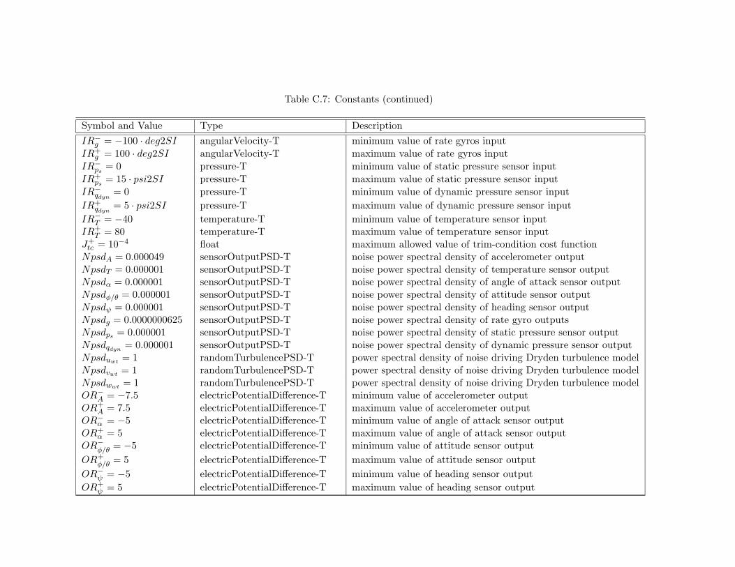
Table C.7: Constants (continued)
Symbol and Value Type DescriptionIR−
g = −100 · deg2SI angularVelocity-T minimum value of rate gyros inputIR+
g = 100 · deg2SI angularVelocity-T maximum value of rate gyros inputIR−
ps= 0 pressure-T minimum value of static pressure sensor input
IR+ps
= 15 · psi2SI pressure-T maximum value of static pressure sensor inputIR−
qdyn= 0 pressure-T minimum value of dynamic pressure sensor input
IR+qdyn
= 5 · psi2SI pressure-T maximum value of dynamic pressure sensor inputIR−
T = −40 temperature-T minimum value of temperature sensor inputIR+
T = 80 temperature-T maximum value of temperature sensor inputJ+
tc = 10−4 float maximum allowed value of trim-condition cost functionNpsdA = 0.000049 sensorOutputPSD-T noise power spectral density of accelerometer outputNpsdT = 0.000001 sensorOutputPSD-T noise power spectral density of temperature sensor outputNpsdα = 0.000001 sensorOutputPSD-T noise power spectral density of angle of attack sensor outputNpsdφ/θ = 0.000001 sensorOutputPSD-T noise power spectral density of attitude sensor outputNpsdψ = 0.000001 sensorOutputPSD-T noise power spectral density of heading sensor outputNpsdg = 0.0000000625 sensorOutputPSD-T noise power spectral density of rate gyro outputsNpsdps = 0.000001 sensorOutputPSD-T noise power spectral density of static pressure sensor outputNpsdqdyn
= 0.000001 sensorOutputPSD-T noise power spectral density of dynamic pressure sensor outputNpsduwt = 1 randomTurbulencePSD-T power spectral density of noise driving Dryden turbulence modelNpsdvwt = 1 randomTurbulencePSD-T power spectral density of noise driving Dryden turbulence modelNpsdwwt = 1 randomTurbulencePSD-T power spectral density of noise driving Dryden turbulence modelOR−
A = −7.5 electricPotentialDifference-T minimum value of accelerometer outputOR+
A = 7.5 electricPotentialDifference-T maximum value of accelerometer outputOR−
α = −5 electricPotentialDifference-T minimum value of angle of attack sensor outputOR+
α = 5 electricPotentialDifference-T maximum value of angle of attack sensor outputOR−
φ/θ = −5 electricPotentialDifference-T minimum value of attitude sensor outputOR+
φ/θ = 5 electricPotentialDifference-T maximum value of attitude sensor outputOR−
ψ = −5 electricPotentialDifference-T minimum value of heading sensor outputOR+
ψ = 5 electricPotentialDifference-T maximum value of heading sensor output
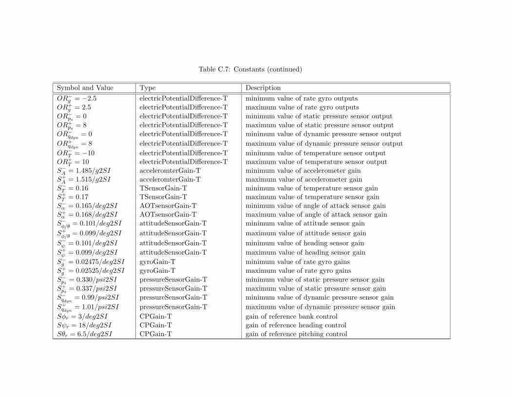
Table C.7: Constants (continued)
Symbol and Value Type DescriptionOR−
g = −2.5 electricPotentialDifference-T minimum value of rate gyro outputsOR+
g = 2.5 electricPotentialDifference-T maximum value of rate gyro outputsOR−
ps= 0 electricPotentialDifference-T minimum value of static pressure sensor output
OR+ps
= 8 electricPotentialDifference-T maximum value of static pressure sensor outputOR−
qdyn= 0 electricPotentialDifference-T minimum value of dynamic pressure sensor output
OR+qdyn
= 8 electricPotentialDifference-T maximum value of dynamic pressure sensor outputOR−
T = −10 electricPotentialDifference-T minimum value of temperature sensor outputOR+
T = 10 electricPotentialDifference-T maximum value of temperature sensor outputS−
A = 1.485/g2SI acceleromterGain-T minimum value of accelerometer gainS+
A = 1.515/g2SI acceleromterGain-T maximum value of accelerometer gainS−
T = 0.16 TSensorGain-T minimum value of temperature sensor gainS+
T = 0.17 TSensorGain-T maximum value of temperature sensor gainS−
α = 0.165/deg2SI AOTsensorGain-T minimum value of angle of attack sensor gainS+
α = 0.168/deg2SI AOTsensorGain-T maximum value of angle of attack sensor gainS−
φ/θ = 0.101/deg2SI attitudeSensorGain-T minimum value of attitude sensor gainS+
φ/θ = 0.099/deg2SI attitudeSensorGain-T maximum value of attitude sensor gainS−
ψ = 0.101/deg2SI attitudeSensorGain-T minimum value of heading sensor gainS+
ψ = 0.099/deg2SI attitudeSensorGain-T maximum value of heading sensor gainS−
g = 0.02475/deg2SI gyroGain-T minimum value of rate gyro gainsS+
g = 0.02525/deg2SI gyroGain-T maximum value of rate gyro gainsS−
ps= 0.330/psi2SI pressureSensorGain-T minimum value of static pressure sensor gain
S+ps
= 0.337/psi2SI pressureSensorGain-T maximum value of static pressure sensor gainS−
qdyn= 0.99/psi2SI pressureSensorGain-T minimum value of dynamic pressure sensor gain
S+qdyn
= 1.01/psi2SI pressureSensorGain-T maximum value of dynamic pressure sensor gainSφr = 3/deg2SI CPGain-T gain of reference bank controlSψr = 18/deg2SI CPGain-T gain of reference heading controlSθr = 6.5/deg2SI CPGain-T gain of reference pitching control

Table C.7: Constants (continued)
Symbol and Value Type DescriptionTs = 1/50 time-T sampling timeVth = 0 CPOutput-T threshold value of control switchesφ−
r = −30 · deg2SI angle-T minimum value of roll angle referenceφ+
r = 30 · deg2SI angle-T maximum value of roll angle referenceψ−
r = 0 · deg2SI angle-T minimum value of heading referenceψ+
r = 360 · deg2SI angle-T maximum value of heading referenceθ−r = −8 · deg2SI angle-T minimum value of pitch angle referenceθ+r = 18 · deg2SI angle-T maximum value of pitch angle reference
n+ = 2300 · RPM2SI engineSpeed-T maximum value of engine speedp+
z = 26 · inHg2SI pressure-T maximum value of engine manifold pressureP+ = 450 · hp2SI power-T maximum value of engine power
Ar =
−9.2131 4.8550 14.08890 0 1.0000
0.6720 −809.2957 −50.3478
state matrix for small perturbation model of rudder actuator
Br =
24.5709 0.00420 0
7.5436 −0.7416
control matrix for small perturbation model of rudder actuator
Cr =[
0 57.2958 0], Dr =
[0 0
]output matrices for small perturbation model of rudder actuator
Aa =
−10.5970 −3.2326 −9.25150 0 1.0000
1.0877 −684.8274 −19.6229
state matrix for small perturbation model of aileron actuator
Ba =
27.4630 −0.00540 0
3.0187 −1.1144
control matrix for small perturbation model of aileron actuator
Ca =[
0 83.8753 0], Da =
[0 0
]output matrices for small perturbation model of aileron actuator
Table C.7: Constants (continued)
Symbol and Value Type Description
Ae =
−10.9510 8.8068 25.18560 0 1.0000
7.3446 −809.7962 −20.1972
state matrix for small perturbation model of elevator actuator
Be =
25.1568 0.00050 0
5.8694 −0.0516
control matrix for small perturbation model of elevator actuator
Ce =[
0 67.1621 0], De =
[0 0
]output matrices for small perturbation model of elevator actuator
Ce1 = 0.08696, Ce2 = 191.18, Ce3 = 0.7355,Ce4 = −326.5, Ce5 = 0.00412, Ce6 = 7.4, engine model coefficientsCe7 = 2010, Ce8 = 408.0, Ce9 = −0.0965
FCS software constantsKr = −4 float constant of asymmetric autopilotKa i = 0.25 frequency-T integration gain of asymmetric autopilotKs i = 0.5 frequency-T integration gain of symmetric autopilot∆φAL = 0.03491 angle-T correction term in ALH autopilot∆φPAH = 0 angle-T correction term in PAH autopilot∆φ+
V = 3.75 · deg2SI angle-T max allowed value for ∆φ∆φ−
V = −3.75 · deg2SI angle-T min allowed value for ∆φ∆φ+
r = 30 · deg2SI angle-T ∆φr minimum value∆φ−
r = −30 · deg2SI angle-T ∆φr minimum value∆θ+
V = 2 · deg2SI angle-T max allowed value for ∆θ∆θ−V = −2 · deg2SI angle-T min allowed value for ∆θ∆θ+
r = 18 · deg2SI angle-T ∆θr minimum value∆θ−r = −8 · deg2SI angle-T ∆θr minimum valuedar = −0.165 float turn-coordination loop constant of asymmetric autopilotl−a = −1 · deg2SI angle-T inferior limit of asymmetric autopilot integratorl+a = 1 · deg2SI angle-T superior limit of asymmetric autopilot integrator
Table C.7: Constants (continued)
Symbol and Value Type Descriptionl−s1 = −10 · deg2SI angle-T inferior limit of symmetric autopilot integratorl+s1 = 10 · deg2SI angle-T superior limit of symmetric autopilot integratorl−s2 = −20 · deg2SI angle-T inferior limit of ALH autopilotl+s2 = 20 · deg2SI angle-T superior limit of ALH autopilot
Conversion factorspsi2SI = 6894.757 float conversion factor from psi to Pafoot2SI = 0.3048 float conversion factor from foot to mdeg2SI = π/180 float conversion factor from degree to radg2SI = 9.80665 float conversion factor from g to m · s−2
RPM2SI = 0.1047198 float conversion factor from RPM to rad · s−1
inHg2SI = 3386.389 float conversion factor from inHg to Pahp2SI = 745.6999 float conversion factor from hp to J · s−1

Table C.8: Quantified variables
Symbol Type DescriptionCX0() time-T → stabilityDerivative-T actual value of stability derivative of force along XB-axisCXα() time-T → stabilityDerivative-T actual value of stability derivative of force along XB-axisCXq() time-T → stabilityDerivative-T actual value of stability derivative of force along XB-axisCXαδf
() time-T → controlDerivative-T actual value of control derivative of force along XB-axisCXα2 () time-T → stabilityDerivative-T actual value of stability derivative of force along XB-axisCXα3 () time-T → stabilityDerivative-T actual value of stability derivative of force along XB-axisCXδf
() time-T → controlDerivative-T actual value of control derivative of force along XB-axisCXδr
() time-T → controlDerivative-T actual value of control derivative of force along XB-axisCY0() time-T → stabilityDerivative-T actual value of stability derivative of force along YB-axisCYβ
() time-T → stabilityDerivative-T actual value of stability derivative of force along YB-axisCYp() time-T → stabilityDerivative-T actual value of stability derivative of force along YB-axisCYr() time-T → stabilityDerivative-T actual value of stability derivative of force along YB-axisCYαδr
() time-T → controlDerivative-T actual value of control derivative of force along YB-axisCYδa
() time-T → controlDerivative-T actual value of control derivative of force along YB-axisCYδr
() time-T → controlDerivative-T actual value of control derivative of force along YB-axisCYβ
() time-T → stabilityDerivative-T actual value of stability derivative of force along YB-axisCZ0() time-T → stabilityDerivative-T actual value of stability derivative of force along ZB-axisCZα() time-T → stabilityDerivative-T actual value of stability derivative of force along ZB-axisCZq() time-T → stabilityDerivative-T actual value of stability derivative of force along ZB-axisCZαδf
() time-T → controlDerivative-T actual value of control derivative of force along ZB-axisCZα3 () time-T → stabilityDerivative-T actual value of stability derivative of force along ZB-axisCZβ2δe
() time-T → controlDerivative-T actual value of control derivative of force along ZB-axisCZδe
() time-T → controlDerivative-T actual value of control derivative of force along ZB-axisCZδf
() time-T → controlDerivative-T actual value of control derivative of force along ZB-axisCl0() time-T → stabilityDerivative-T actual value of stability derivative of moment about XB-axisClβ () time-T → stabilityDerivative-T actual value of stability derivative of moment about XB-axisClp() time-T → stabilityDerivative-T actual value of stability derivative of moment about XB-axisClr() time-T → stabilityDerivative-T actual value of stability derivative of moment about XB-axis
Table C.8: Quantified variables (continued)
Symbol Type DescriptionClαδa
() time-T → controlDerivative-T actual value of control derivative of moment about XB-axisClδa
() time-T → controlDerivative-T actual value of control derivative of moment about XB-axisClδr
() time-T → controlDerivative-T actual value of control derivative of moment about XB-axisCm0() time-T → stabilityDerivative-T actual value of stability derivative of moment about YB-axisCmα() time-T → stabilityDerivative-T actual value of stability derivative of moment about YB-axisCmq() time-T → stabilityDerivative-T actual value of stability derivative of moment about YB-axisCmr() time-T → stabilityDerivative-T actual value of stability derivative of moment about YB-axisCmα2 () time-T → stabilityDerivative-T actual value of stability derivative of moment about YB-axisCmβ2 () time-T → stabilityDerivative-T actual value of stability derivative of moment about YB-axisCmδe
() time-T → controlDerivative-T actual value of control derivative of moment about YB-axisCmδf
() time-T → controlDerivative-T actual value of control derivative of moment about YB-axisCn0() time-T → stabilityDerivative-T actual value of stability derivative of moment about ZB-axisCnβ
() time-T → stabilityDerivative-T actual value of stability derivative of moment about ZB-axisCnp() time-T → stabilityDerivative-T actual value of stability derivative of moment about ZB-axisCnq() time-T → stabilityDerivative-T actual value of stability derivative of moment about ZB-axisCnr() time-T → stabilityDerivative-T actual value of stability derivative of moment about ZB-axisCnβ3 () time-T → stabilityDerivative-T actual value of stability derivative of moment about ZB-axisCnδa
() time-T → controlDerivative-T actual value of control derivative of moment about ZB-axisCnδr
() time-T → controlDerivative-T actual value of control derivative of moment about ZB-axisIx() time-T → momentOfInertia-T actual value of moment of inertia along XB-axisIy() time-T → momentOfInertia-T actual value of moment of inertia along YB-axisIz() time-T → momentOfInertia-T actual value of moment of inertia along ZB-axisJxy() time-T → productOfInertia-T actual value of product of inertia in XBYB-planeJxz() time-T → productOfInertia-T actual value of product of inertia in XBZB-planeJyz() time-T → productOfInertia-T actual value of product of inertia in YBZB-planeP () time-T → power-T engine powerSAx accelerometerGain-T actual value of Ax accelerometer gainSAy accelerometerGain-T actual value of Ay accelerometer gain

Table C.8: Quantified variables (continued)
Symbol Type DescriptionSAz accelerometerGain-T actual value of Az accelerometer gainST TSensorGain-T actual value of temperature sensor gainSα AOTSensorGain-T actual value of angle of attack sensor gainSφ attitudeSensorGain-T actual value of roll attitude sensor gainSψ attitudeSensorGain-T actual value of heading sensor gainSθ attitudeSensorGain-T actual value of pitch attitude sensor gainSps pressureSensorGain-T actual value of static pressure sensor gainSp gyroGain-T actual value of roll rate gyro gainSqdyn
pressureSensorGain-T actual value of dynamic pressure sensor gainSq gyroGain-T actual value of pitch rate gyro gainSr gyroGain-T actual value of yaw rate gyro gainxa() array of float state vector of small perturbation aileron modelxe() array of float state vector of small perturbation elevator modelxr() array of float state vector of small perturbation rudder modelνAx() time-T → accelerometerOutput-T instance of Ax accelerometer output noiseνAy() time-T → accelerometerOutput-T instance of Ayaccelerometer output noiseνAz() time-T → accelerometerOutput-T instance of Azaccelerometer output noiseνT () time-T → TSensorOutput-T instance of temperature sensor output noiseνα() time-T → AOTSensorOutput-T instance of angle of attack sensor output noiseνφ() time-T → attitudeSensorOutput-T instance of roll attitude sensor output noiseνψ() time-T → headingSensorOutput-T instance of heading sensor output noiseνθ() time-T → attitudeSensorOutput-T instance of pitch attitude sensor output noiseνps() time-T → pressureSensorOutput-T instance of static pressure sensor output noiseνp() time-T → gyroOutput-T instance of roll rate gyro output noiseνqdyn
() time-T → pressureSensorOutput-T instance of dynamic pressure sensor output noiseνq() time-T → gyroOutput-T instance of pitch rate gyro output noiseνr() time-T → gyroOutput-T instance of yaw rate gyro output noiseνuwt() time-T → float instance of noise driving Dryden turbulence model
Table C.8: Quantified variables (continued)
Symbol Type Descriptionνvwt() time-T → float instance of noise driving Dryden turbulence modelνwwt() time-T → float instance of noise driving Dryden turbulence modela, b float coefficients used within the trim-condition requirementbiasAx accelerometerBias-T actual value of Ax accelerometer biasbiasAy accelerometerBias-T actual value of Ay accelerometer biasbiasAz accelerometerBias-T actual value of Az accelerometer biasbiasT TSensorBias-T actual value of temperature sensor biasbiasα AOTSensorBias-T actual value of angle of attack sensor biasbiasφ attitudeSensorBias-T actual value of roll attitude sensor biasbiasψ headingSensorBias-T actual value of heading sensor biasbiasθ attitudeSensorBias-T actual value of pitch attitude sensor biasbiasps psSensorBias-T actual value of static pressure sensor biasbiasp gyroBias-T actual value of roll rate gyro biasbiasqdyn
qdynSensorBias-T actual value of dynamic pressure sensor biasbiasq gyroBias-T actual value of pitch rate gyro biasbiasr gyroBias-T actual value of yaw rate gyro biasdpt() time-T → float non-dimensional pressure increase in propeller slipstreamk integer counterm() time-T → force-T actual airplane weightt, t1, t2, t3, t4 time-T continuous time instant

Table C.9: Auxiliary terms
Symbol and expression in terms of basequantities
Type Description
Auxiliary termsFx() = Xasd
()+Xacd()+Xp()+Xgr()+Xw() time-T → force-T total force along XB-axis
Fy() = Yasd() + Yacd
() + Yp() + Ygr() + Yw() time-T → force-T total force along YB-axisFz() = Zasd
() + Zacd() + Zp() + Zgr() + Zw() time-T → force-T total force along ZB-axis
I1() = Iy()Iz() − J2yz() time-T → inertiaParam-T inertia parameter for moment equations
I2() = Jxy()Iz() + Jyz()Jxz() time-T → inertiaParam-T inertia parameter for moment equationsI3() = Jxy()Jyz() + Iy()Jxz() time-T → inertiaParam-T inertia parameter for moment equationsI4() = Ix()Iz() − J2
xz() time-T → inertiaParam-T inertia parameter for moment equationsI5() = Ix()Jyz() + Jxy()Jxz() time-T → inertiaParam-T inertia parameter for moment equationsI6() = Ix()Iy() − J2
xy() time-T → inertiaParam-T inertia parameter for moment equations|I()| = Ix()Iy()Iz() − 2Jxy()Jxz()Jyz() −Ix()J2
yz() − Iy()J2xz() − Iz()J2
xy()time-T → inertiaParam-T inertia parameter for moment equations
Jtc(( Va(0), α(0), β(0), p(0), q(0), r(0) )=CVa V 2
a (0) + Cαβ ( α2(0) + β2(0) ) +Cpqr (p2(0) + q2(0) + r2(0) )
(acceleration-T,angularVelocity-T,angularVelocity-T,angularAcceleration-T,angularAcceleration-T,angularAcceleration-T) →float
cost function for trim-condition
KH(Va) = (−1 · 10−4V 2a + 0.015Va −
0.5975)π/180airspeed-T → float proportional gain of ALH autopilot
Kφ(Va) = 9.75 · 10−4V 2a − 0.108Va + 2.335625 airspeed-T → float proportional gain of asymmetric autopilot
Kψ(Va) = 0.05Va − 1.1 airspeed-T → float proportional gain of HH/HS autopilotKθ(Va) = 1.375 · 10−3V 2
a + 0.1575Va − 4.8031 airspeed-T → float proportional gain of PAH autopilotKθ(Va) = 1.375 · 10−3V 2
a + 0.1575Va − 4.8031 airspeed-T → float proportional gain of ALH and ALS autopilotKd(Va) = −2.5 · 10−3Va + 0.2875 airspeed-T → float proportional gain of ALH and ALS autopilot
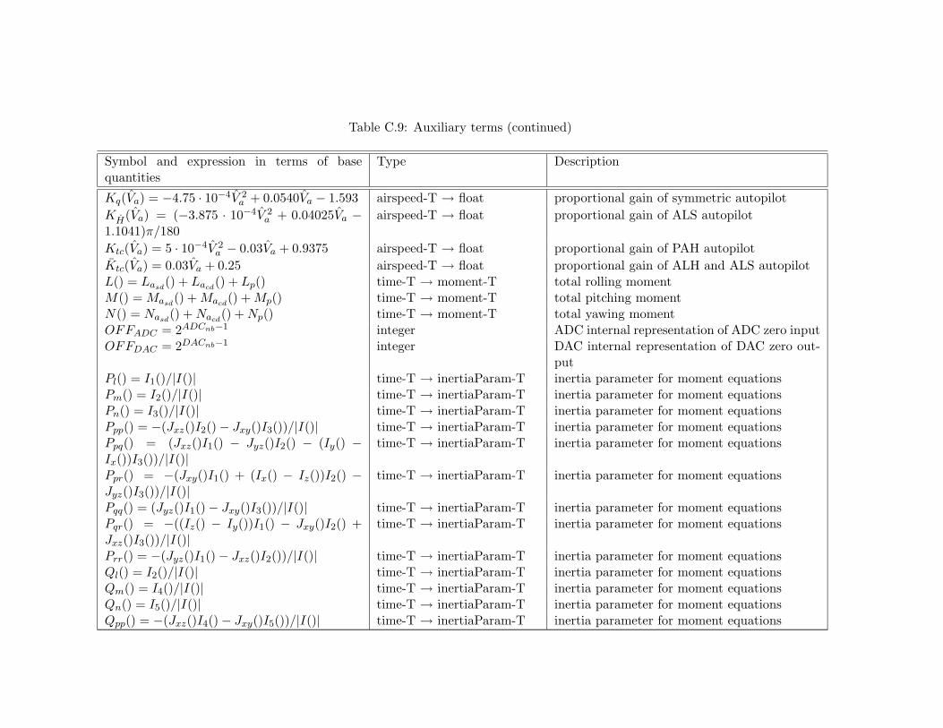
Table C.9: Auxiliary terms (continued)
Symbol and expression in terms of basequantities
Type Description
Kq(Va) = −4.75 · 10−4V 2a + 0.0540Va − 1.593 airspeed-T → float proportional gain of symmetric autopilot
KH(Va) = (−3.875 · 10−4V 2a + 0.04025Va −
1.1041)π/180airspeed-T → float proportional gain of ALS autopilot
Ktc(Va) = 5 · 10−4V 2a − 0.03Va + 0.9375 airspeed-T → float proportional gain of PAH autopilot
Ktc(Va) = 0.03Va + 0.25 airspeed-T → float proportional gain of ALH and ALS autopilotL() = Lasd
() + Lacd() + Lp() time-T → moment-T total rolling moment
M() = Masd() + Macd
() + Mp() time-T → moment-T total pitching momentN() = Nasd
() + Nacd() + Np() time-T → moment-T total yawing moment
OFFADC = 2ADCnb−1 integer ADC internal representation of ADC zero inputOFFDAC = 2DACnb−1 integer DAC internal representation of DAC zero out-
putPl() = I1()/|I()| time-T → inertiaParam-T inertia parameter for moment equationsPm() = I2()/|I()| time-T → inertiaParam-T inertia parameter for moment equationsPn() = I3()/|I()| time-T → inertiaParam-T inertia parameter for moment equationsPpp() = −(Jxz()I2() − Jxy()I3())/|I()| time-T → inertiaParam-T inertia parameter for moment equationsPpq() = (Jxz()I1() − Jyz()I2() − (Iy() −Ix())I3())/|I()|
time-T → inertiaParam-T inertia parameter for moment equations
Ppr() = −(Jxy()I1() + (Ix() − Iz())I2() −Jyz()I3())/|I()|
time-T → inertiaParam-T inertia parameter for moment equations
Pqq() = (Jyz()I1() − Jxy()I3())/|I()| time-T → inertiaParam-T inertia parameter for moment equationsPqr() = −((Iz() − Iy())I1() − Jxy()I2() +Jxz()I3())/|I()|
time-T → inertiaParam-T inertia parameter for moment equations
Prr() = −(Jyz()I1() − Jxz()I2())/|I()| time-T → inertiaParam-T inertia parameter for moment equationsQl() = I2()/|I()| time-T → inertiaParam-T inertia parameter for moment equationsQm() = I4()/|I()| time-T → inertiaParam-T inertia parameter for moment equationsQn() = I5()/|I()| time-T → inertiaParam-T inertia parameter for moment equationsQpp() = −(Jxz()I4() − Jxy()I5())/|I()| time-T → inertiaParam-T inertia parameter for moment equations

Table C.9: Auxiliary terms (continued)
Symbol and expression in terms of basequantities
Type Description
Qpq() = (Jxz()I2() − JyzI4() − (Iy() −Ix())I5())/|I()|
time-T → inertiaParam-T inertia parameter for moment equations
Qpr() = −(Jxy()I2() + (Ix() − Iz())I4() −Jyz()I5())/|I()|
time-T → inertiaParam-T inertia parameter for moment equations
Qqq() = (Jyz()I2() − Jxy()I5())/|I()| time-T → inertiaParam-T inertia parameter for moment equationsQqr() = −((Iz() − Iy())I2() − Jxy()I4() +Jxz()I5())/|I()|
time-T → inertiaParam-T inertia parameter for moment equations
Qrr() = −(Jyz()I2() − Jxz()I4())/|I()| time-T → inertiaParam-T inertia parameter for moment equationsRl() = I3()/|I()| time-T → inertiaParam-T inertia parameter for moment equationsRm() = I5()/|I()| time-T → inertiaParam-T inertia parameter for moment equationsRn() = I6()/|I()| time-T → inertiaParam-T inertia parameter for moment equationsRpp() = −(Jxz()I5() − Jxy()I6())/|I()| time-T → inertiaParam-T inertia parameter for moment equationsRpq() = (Jxz()I3() − Jyz()I5() − (Iy() −Ix())I6())/|I()|
time-T → inertiaParam-T inertia parameter for moment equations
Rpr() = −(Jxy()I3() + (Ix() − Iz())I5() −Jyz()I6())/|I()|
time-T → inertiaParam-T inertia parameter for moment equations
Rqq() = (Jyz()I3() − Jxy()I6())/|I()| time-T → inertiaParam-T inertia parameter for moment equationsRqr() = −((Iz() − Iy())I3() − Jxy()I5() +Jxz()I6())/|I()|
time-T → inertiaParam-T inertia parameter for moment equations
Rrr() = −(Jyz()I3() − Jxz()I5())/|I()| time-T → inertiaParam-T inertia parameter for moment equationsSADC = 2ADCnb−1
DACV +−DACV − float ADC resolution
SDAC = 2DACnb−1DACV +−DACV − float DAC resolution
huwt() = F−1
{σu
√2LuVa(t)
1(1+ Lu
Va(t)jω
) }time-T → turbulence-T filter implementing Dryden turbulence model
hvwt() = F−1
{σv
√Lv
Va(t)
1+√
3 LvVa(t)
jω(1+ Lv
Va(t)jω
)2
}time-T → turbulence-T filter implementing Dryden turbulence model
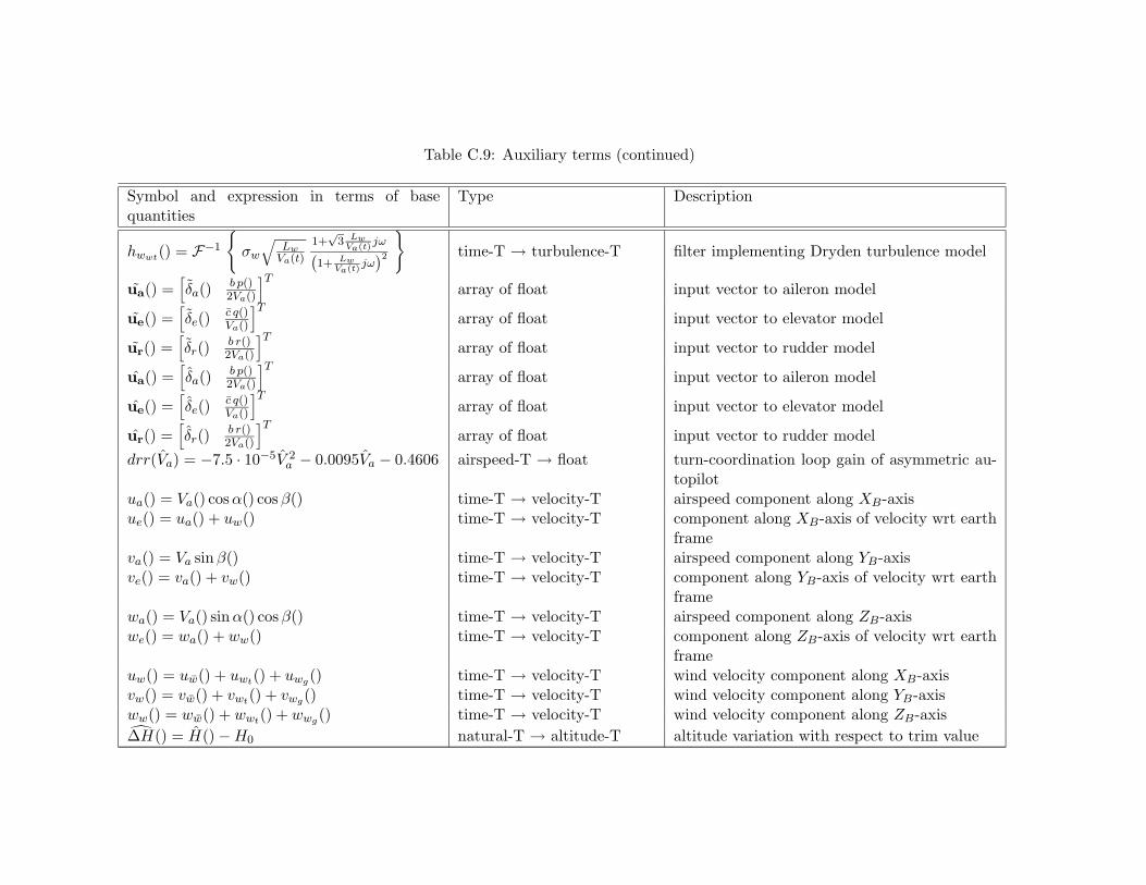
Table C.9: Auxiliary terms (continued)
Symbol and expression in terms of basequantities
Type Description
hwwt() = F−1
{σw
√Lw
Va(t)
1+√
3 LwVa(t)
jω(1+ Lw
Va(t)jω
)2
}time-T → turbulence-T filter implementing Dryden turbulence model
ua() =[δa()
b p()2Va()
]Tarray of float input vector to aileron model
ue() =[δe()
c q()Va()
]Tarray of float input vector to elevator model
ur() =[δr()
b r()2Va()
]Tarray of float input vector to rudder model
ua() =[δa()
b p()2Va()
]Tarray of float input vector to aileron model
ue() =[δe()
c q()Va()
]Tarray of float input vector to elevator model
ur() =[δr()
b r()2Va()
]Tarray of float input vector to rudder model
drr(Va) = −7.5 · 10−5V 2a − 0.0095Va − 0.4606 airspeed-T → float turn-coordination loop gain of asymmetric au-
topilotua() = Va() cos α() cos β() time-T → velocity-T airspeed component along XB-axisue() = ua() + uw() time-T → velocity-T component along XB-axis of velocity wrt earth
frameva() = Va sinβ() time-T → velocity-T airspeed component along YB-axisve() = va() + vw() time-T → velocity-T component along YB-axis of velocity wrt earth
framewa() = Va() sin α() cos β() time-T → velocity-T airspeed component along ZB-axiswe() = wa() + ww() time-T → velocity-T component along ZB-axis of velocity wrt earth
frameuw() = uw() + uwt() + uwg() time-T → velocity-T wind velocity component along XB-axisvw() = vw() + vwt() + vwg() time-T → velocity-T wind velocity component along YB-axisww() = ww() + wwt() + wwg() time-T → velocity-T wind velocity component along ZB-axis∆H() = H() − H0 natural-T → altitude-T altitude variation with respect to trim value

Table C.9: Auxiliary terms (continued)
Symbol and expression in terms of basequantities
Type Description
∆δa() = δa() − δa0 natural-T →aileronDeflection-T
aileron defliection variation with respect to trimvalue
∆δe() = δe() − δe0 natural-T →elevatorDeflection-T
elevator defliection variation with respect totrim value
∆δr() = δr() − δr0 natural-T →rudderDeflection-T
rudder defliection variation with respect to trimvalue
∆φ() = φ() − φ0 natural-T → angle-T bank angle variation with respect to trim value∆φr() = φr() − φr0 natural-T → bankReference-
Tbank reference variation with respect to trimvalue
∆ψ() = ψ() − ψ0 natural-T → angle-T heading variation with respect to trim value∆ψr() = ψr() − ψr0 natural-T →
headingReference-Theading reference variation with respect to trimvalue
∆θ() = θ() − θ0 natural-T → angle-T pitch angle variation with respect to trim value∆θr() = θr() − θr0 natural-T → pitchReference-
Tpitch reference variation with respect to trimvalue
Auxiliary functions, operators, and predicates
constRef(f(), t1, t2) = ∃ k ∀ t(
t1 ≤ t ≤t2 ⇒ f(t) = k
) not specified predicate that evaluates true if f() is constantthroughout the time interval [t1, t2]
engaged(SW (), t1, t2) = ∃Tε
(0 < Tε < ∞ ∧
∀ t(
t1 − Tε < t < t1 ⇒ SW (t) = OFF)
∧ ∀ t(
t1 ≤ t < t2 ⇒ SW (t) = ON))
(switch-T, time-T, time-T)→ boolean
predicate that evaluates true only if the switchSW () is engaged at t = t1 and stays engagedthroughout the time interval [t1, t2]
turb(t1, t2) = ¬ ∀ t(
t1 ≤ t ≤ t2 ⇒ uwt(t) =0 ∧ wwt(t) = 0 ∧ wwt(t) = 0 ∧ uwg(t) =0 ∧ wwg(t) = 0 ∧ wwg(t) = 0 ∧
)(time-T, time-T) → boolean predicate that evaluates true if random and dis-
crete turbulence wind components are not zero

Table C.9: Auxiliary terms (continued)
Symbol and expression in terms of basequantities
Type Description
whileEngaged(SW (), t1, t2) = ∀ t(
t1 ≤ t <
t2 ⇒ SW (t) = ON) (switch-T, time-T, time-T)
→ booleanpredicate that evaluates true only if the switchSW () is engaged throughout the time interval[t1, t2]
whiteNoise(ν(), Npsd) not specified predicate that evaluates true if ν() is whitenoise with Power Spectral Density Npsd
p1() ' p2() ⇔ E{a(t)a(t+τ)} = E{b(t)b(t+τ)}
not specified equivalence operator between stochastic pro-cesses
z(f(k)) = f(k + 1) not specified one step forward operator[x
]b
a=
x : a < x < ba : a ≤ xb : x ≤ b
not specified crop operator
RMS(f(), t1, t2) =√
1t2−t1
∫ t2t1
f2(t)dt not specified Root Mean Square value of a function over theinterval [t1, t2]⌊
x⌋= y ⇔ y ∈ N ∧ y < x ∧ ∀n
(n ∈
N ∧ n > y ⇒ n > x) not specified quantization to closest integer

Table C.10: Data-types
Type ID Base type Range SI symbol DescriptionADCinput-T electricPotentialDifference-T [ADCV − , ADCV + ] inherited input to A/D cardADCoutput-T integer [0, 2ADCnb) inherited output from A/D cardAOT-T angle-T [−10, 30] · deg2SI inherited angle of attackAOTSensorBias-T electricPotentialDifference-T [BIAS−
α , BIAS+α ] inherited angle of attack sensor output
AOTSensorGain-T angularSensorGain-T [S−α , S+
α ] inherited gain of angle of attack sensorAOTSensorOutput-T electricPotentialDifference-T [OR−
α , OR+α ] inherited angle of attack sensor output
CPGain-T float (−∞, +∞) V · rad−1 gain of knob controls from con-trol panel
CPOutput-T electricPotentialDifference-T [CP−, CP+] inherited output of controls from controlpanel
DACinput-T integer [0, 2DACnb) inherited input to D/A cardDACoutput-T electricPotentialDifference-T [DACV − , DACV + ] inherited output from D/A cardPCUInput-T electricPotentialDifference-T [PCU−, PCU+] inherited power control unit inputTCWeight-T float-T (−∞, +∞) notspecified trim condition weightTSensorBias-T electricPotentialDifference-T [BIAS−
T , BIAS+T ] inherited temperature sensor output
biasTSensorGain-T temperatureSensorGain-T [S−
T , S+T ] inherited temperature sensor gain
TSensorOutput-T electricPotentialDifference-T [OR−T , OR+
T ] inherited temperature sensor outputaccelerationSensorGain-T float (−∞, +∞) V · s · m−1 acceleration sensor gainacceleration-T float (−∞, +∞) m · s−1 linear accelerationaccelerometerBias-T electricPotentialDifference-T [BIAS−
A , BIAS+A ] inherited accelerometer output bias
accelerometerGain-T accelerationSensorGain-T [S−A , S+
A ] inherited accelerometer gainaccelerometerOutput-T electricPotentialDifference-T [OR−
A, OR+A] inherited accelerometer output
aileronDeflection-T angle-T [δ−a , δ+a ] inherited aileron deflection
airspeed-T velocity [35, 65] inherited air velocityaltitude-T length-T [2000, 10000] ·
foot2SIinherited barometric altitude
angle-T float (−∞, +∞) rad angle
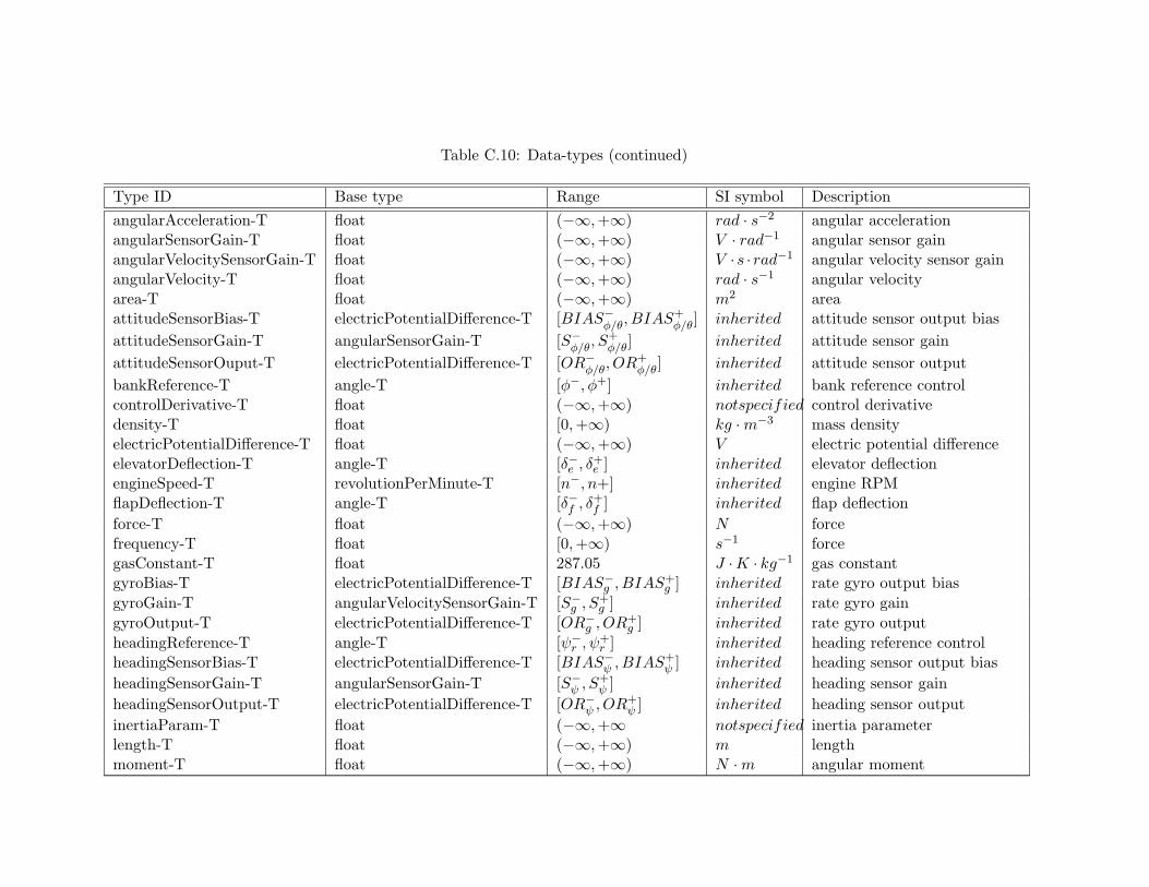
Table C.10: Data-types (continued)
Type ID Base type Range SI symbol DescriptionangularAcceleration-T float (−∞, +∞) rad · s−2 angular accelerationangularSensorGain-T float (−∞, +∞) V · rad−1 angular sensor gainangularVelocitySensorGain-T float (−∞, +∞) V ·s · rad−1 angular velocity sensor gainangularVelocity-T float (−∞, +∞) rad · s−1 angular velocityarea-T float (−∞, +∞) m2 areaattitudeSensorBias-T electricPotentialDifference-T [BIAS−
φ/θ, BIAS+φ/θ] inherited attitude sensor output bias
attitudeSensorGain-T angularSensorGain-T [S−φ/θ, S
+φ/θ] inherited attitude sensor gain
attitudeSensorOuput-T electricPotentialDifference-T [OR−φ/θ, OR+
φ/θ] inherited attitude sensor outputbankReference-T angle-T [φ−, φ+] inherited bank reference controlcontrolDerivative-T float (−∞, +∞) notspecified control derivativedensity-T float [0, +∞) kg · m−3 mass densityelectricPotentialDifference-T float (−∞, +∞) V electric potential differenceelevatorDeflection-T angle-T [δ−e , δ+
e ] inherited elevator deflectionengineSpeed-T revolutionPerMinute-T [n−, n+] inherited engine RPMflapDeflection-T angle-T [δ−f , δ+
f ] inherited flap deflectionforce-T float (−∞, +∞) N forcefrequency-T float [0, +∞) s−1 forcegasConstant-T float 287.05 J ·K · kg−1 gas constantgyroBias-T electricPotentialDifference-T [BIAS−
g , BIAS+g ] inherited rate gyro output bias
gyroGain-T angularVelocitySensorGain-T [S−g , S+
g ] inherited rate gyro gaingyroOutput-T electricPotentialDifference-T [OR−
g , OR+g ] inherited rate gyro output
headingReference-T angle-T [ψ−r , ψ+
r ] inherited heading reference controlheadingSensorBias-T electricPotentialDifference-T [BIAS−
ψ , BIAS+ψ ] inherited heading sensor output bias
headingSensorGain-T angularSensorGain-T [S−ψ , S+
ψ ] inherited heading sensor gainheadingSensorOutput-T electricPotentialDifference-T [OR−
ψ , OR+ψ ] inherited heading sensor output
inertiaParam-T float (−∞, +∞ notspecified inertia parameterlength-T float (−∞, +∞) m lengthmoment-T float (−∞, +∞) N · m angular moment

Table C.10: Data-types (continued)
Type ID Base type Range SI symbol DescriptionmomentOfInertia-T float [0,∞) kg · m2 moment of inertianatural-T integer [0, +∞) notspecified natural numberpercentage-T float [0, 1] notspecified percentagepitchReference-T angle-T [θ−, θ+] inherited pitch reference controlpressureSensorGain-T float (−∞, +∞) V ·N−1 ·m2 pressure sensor gainpower-T float (−∞, +∞) J · s−1 pressurepressure-T float (−∞, +∞) N · m−2 pressureproductOfInertia-T float [0,∞) kg · m2 product of inertiapsSensorBias-T electricPotentialDifference-T [BIAS−
ps, BIAS+
ps] inherited static pressure sensor output
biaspsSensorGain-T pressureSensorGain-T [S−
ps, S+
ps] inherited static pressure sensor gain
psSensorOutput-T electricPotentialDifference-T [OR−ps
, OR+ps
] inherited static pressure sensor outputqdynSensorBias-T electricPotentialDifference-T [BIAS−
qdyn, BIAS+
qdyn] inherited dynamic pressure sensor out-
put biasqdynSensorGain-T pressureSensorGain-T [S−
qdyn, S+
qdyn] inherited dynamic pressure sensor gain
qdynSensorOutput-T electricPotentialDifference-T [OR−qdyn
, OR+qdyn
] inherited dynamic pressure sensor out-put
randomTurbulencePSD-T float [0, +∞) notspecified random turbulence powerspectral density
revolutionPerMinute-T angularVelocity-T [0, +∞) inherited revolution per minuterudderDeflection-T angle-T [δ−r , δ+
r ] inherited rudder deflectionsensorOutputPSD-T float [0, +∞) V 2 · Hz−1 power spectral density of sen-
sor outputstabilityDerivative-T float (−∞, +∞) notspecified stability derivativeswitch-T boolean {ON, OFF} notspecified switch controltemperatureGradient-T float (−∞, +∞) K · m−1 temperature gradient in tropo-
spheretemperatureSensorGain-T float (−∞, +∞) V · K−1 temperature sensor gain

Table C.10: Data-types (continued)
Type ID Base type Range SI symbol Descriptiontemperature-T float (−∞, +∞) K temperaturetime-T float (−∞, +∞) s timevelocity-T float (−∞, +∞) m · s−1 linear velocitywarningLight-T boolean {ON, OFF} notspecified warning lightwarningLightInput-T electricPotentialDifference-T [WL−, WL+] inherited input to warning light