<5* Forestry Commission

An Ecological Site Classification for

Forestry in Great Britain, Duncan Ray

iftpd Jane Fletcher

- . * SB

*• i

Forestry Commission

ARCHIVE

FORESTRY COMMISSION BULLETIN 124

An Ecological Site Classification for Forestry in Great Britain

Graham Pyatt, Duncan Ray and Jane Fletcher

W oodland E co logy B ranch , F ores t Research,N o rth e rn Research S ta tion , R os lin , M id lo th ia n , EH 25 9SY

Edinburgh: Forestry Commission

© Croivn copyright 2001Applications fo r reproduction should be made to HMSO, The Copyright Unit, St Clements House, 2-16 Colegate, Norw ich NR3 1BQ

ISBN 0 85538 418 2

Pyatt, G.; Ray, D.; Fletcher, J. 2001An Ecological Site Classification for Forestry in Great Britain. Bulletin 124. Forestry Commission, Edinburgh.

FDC 542:111.82:(410)

KEYWORDS: Climate, Ecology, Forestry, Indicator plants, Soils, Site types

Acknowledgements

The climatic data used in this work were obtained from the UK Meteorological Office under a licence agreement. We are indebted to Messrs Stewart Wass and George Anderson for their help in this matter. We are grateful to the Climatic Research Unit o f the University o f East Anglia (David Viner and Elaine Barrow) for making available the 10 x 10 gridded datasets under the Climate Impacts Link Project o f the UK Department o f the Environment, Transport and the Regions.

Gary White and Tom Connolly respectively assisted with the GIS and statistical work involved in the preparation o f the ;climatic datasets and Karen Purdy helped in the preparation o f the map o f windiness. We thank the various colleagues in Forest Research who helped with the preparation o f the Figures.

The species suitability criteria have been subjected to the scrutiny and approval o f a panel o f ‘three wise men’, Bill Mason, Head o f Silviculture (North) Branch, Alan Fletcher, former Head o f Tree Improvement Branch and Derek Redfem, former Head o f Pathology (North) Section.

Gary Kerr o f Silviculture and Seed Research Branch and Christopher Quine, Head o f Woodland Ecology Branch, read the draft and suggested many improvements. As former Head o f Woodland Ecology Branch, Simon Hodge guided the progress o f ESC for several years.

ContentsPage

Acknowledgements iiList o f Figures viList o f Tables viiiSummary ixResume xZusammenfassung xiCrynodeb xii

1 Introduction 1

2 Climate 3Importance and choice o f factors 3Warmth 3Wetness 4Windiness 5Continentality 5Winter cold, unseasonable frosts and other winter hazards 5Climatic zones 6

3 Soil moisture regime 8Introduction: moisture and oxygen availability 8Factors affecting soil moisture regime 8Assessment o f soil moisture regime 9

Direct assessment o f soil moisture regime in winter 9Direct assessment o f soil moisture regime in summer 9Adjustment o f soil moisture regime for available water capacity 9Adjustment o f soil moisture regime for soil texture and stoniness 9Adjustment o f soil moisture regime for rooting depth 11Adjustment o f soil moisture regime for aspect and slope 11

4 Soil nutrient regime 12Introduction: nutrient availability 12Factors affecting nutrient availability and their potential modification 12Assessment o f soil nutrient regime 13

Direct assessment o f soil nutrient regime 13

5 Indirect assessment o f soil moisture and nutrient regimes from soiltype, lithology and humus form 15Introduction: forest soil types and nutrient regime 15Local adjustment o f soil moisture regime derived from soil type 16Local adjustment o f soil nutrient regime derived from soil type 16Local adjustment o f soil nutrient regime using humus form 19

6 Indirect assessment o f soil moisture and nutrient regimes from indicator plants 20Introduction: the use o f indicator plants in forestry 20The use o f numerical indicator values 20Use o f indicator plants in ESC 21Assessing soil moisture and nutrient regimes using indicator plants 21

Short-cut method 21Numerical method for assessing soil moisture regime 24Numerical method for assessing soil nutrient regime 24

Method o f obtaining quantitative data on indicator plants for ESC 24

7 Choice o f tree species for ESC site types 27Introduction: species suitability 27Risks 34Timber quality 34Natural regeneration 34

8 Native woodlands for ESC site types 38Introduction: climate and soil suitability 38Linking native woodlands with the soil quality grid 38Separating the communities by climatic zones 39Suitability ranges o f all six ESC site factors 39

References 50

Appendix 1 The assessment o f soil texture and available water capacity 54

Appendix 2 Classification o f humus forms 59

Appendix 3 Description o f soil profile 61Introduction: recording information relevant to soil moisture and nutrient regimes 61Choice o f location 61Thickness o f horizons 61Colour 61Stoniness 61Texture 61Structure 62Consistence 62Roots 62Parent material 62Definitions o f horizons 63

Appendix 4 Forest soil classification 67Check list o f soil groups, types and phases (after Pyatt, 1982) 67

iv

Appendix 5 Nitrogen availability categories in the poorer soils (a fter Taylor, 1991) 70(See Chapter 5)Category A 70Category B 70Category C 70Category D 70

Appendix 6 Glossary o f terms 71

v

List o f Figures

Figures 1-8 between pages 4 and 5 Page

1 The three ‘principal components’ o f Ecological Site Classification

2 Map o f accumulated temperature in Great Britain

3 Map o f moisture deficit in Great Britain

4 Map o f windiness (DAMS) in Great Britain

5 Map o f continentality in Great Britain based on the Conrad index (reduced tosea level)

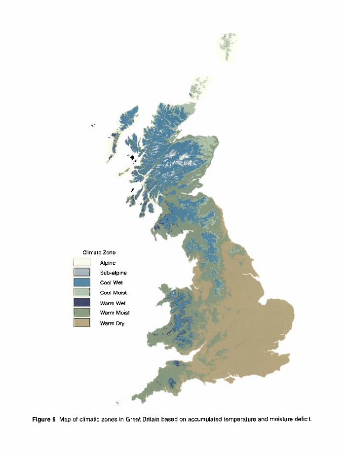
6 Map o f climatic zones in Great Britain based on accumulated temperature and moisture deficit

7 Nine slope shapes combining profile and planform

8 Simplified distribution o f soil types and humus forms on the soil quality grid

9 Suitability o f tree species by accumulated temperature 28

10 Suitability o f tree species by moisture deficit 29

11 Suitability o f tree species by windiness 30

12 Suitability o f tree species by continentality 31

13 Suitability o f tree species by soil moisture regime 32

14 Suitability o f tree species by soil nutrient regime 33

15 Smooth response curves for Sitka sprqcp 35

16 Relative shade tolerance o f tree species in Britain (based on Hill et al., 1999) 36

17 Soil quality and the prospects for natural regeneration o f conifers (after Nixonand Worrell, 1999) 37

18 Ordination o f NVC woodland sub-communities W1-W20 on scales o f F( ‘soil moisture’) and R+N ( ‘soil nutrients’) 39

19 Very suitable soil quality for native oak, ash and alder woodlands in Warm dry and Warm moist climatic zones (the ‘Lowland Zone’ o f FC Bulletin 112(Rodwell and Patterson, 1994)) 40

20 Very suitable soil quality for native beech woodlands in Warm dry and Warmmoist climatic zones (the ‘Lowland Zone’ o f FC Bulletin 112) 41

21 Very suitable soil quality for native woodlands in Warm wet, Cool moist andCool wet climatic zones (the ‘Upland Zone’ o f FC Bulletin 112) 42

22 Very suitable soil quality for native scrub woodlands in the Sub-alpine zone(the ‘Upland juniper zone’ o f FC Bulletin 112) 43

23 Suitability o f native woodlands W1-W20 by accumulated temperature 44

24 Suitability o f native woodlands W1-W20 by moisture deficit 45

25 Suitability o f native woodlands W1-W20 by windiness 46

vi

26

27

28

29

30

31

32

33

34

35

36

47

48

49

55

56

57

58

60

64

65

66

vii

Suitability o f native woodlands W1-W20 by continentality

Suitability o f native woodlands W1-W20 by soil moisture regime

Suitability o f native woodlands W1-W20 by soil nutrient regime

Assessment o f soil texture, method 1 (after Landon, 1988)

Assessment o f soil texture, method 2

Soil texture classes

Estimating the available water capacity (AWC) o f the soil

Key to the humus forms o f Figure 8

Ecological Site Classification: description o f soil profile

Ecological Site Classification: description o f site and vegetation

Abundance charts (after Ontario Institute o f Pedology, 1985)

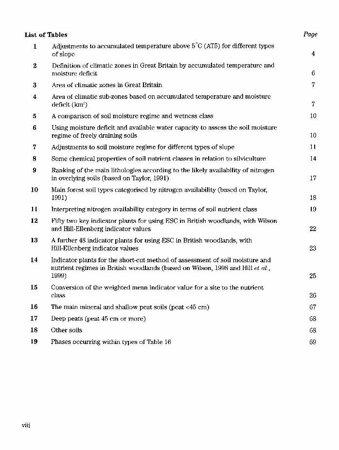
List o f Tables Page

1 Adjustments to accumulated temperature above 5 C (AT5) for different typeso f slope 4

2 Definition o f climatic zones in Great Britain by accumulated temperature andmoisture deficit 6

3 Area o f climatic zones in Great Britain 7

4 Area o f climatic sub-zones based on accumulated temperature and moisturedeficit (km-) 7

5 A comparison o f soil moisture regime and wetness class 10

6 Using moisture deficit and available water capacity to assess the soil moistureregime o f freely draining soils 10

7 Adjustments to soil moisture regime for different types o f slope 11

8 Some chemical properties o f soil nutrient classes in relation to silviculture 14

9 Ranking o f the main lithologies according to the likely availability o f nitrogenin overlying soils (based on Taylor, 1991) 17

10 Main forest soil types categorised by nitrogen availability (based on Taylor,1991) 18

11 Interpreting nitrogen availability category in terms o f soil nutrient class 19

12 Fifty two key indicator plants for using ESC in British woodlands, with Wilsonand Hill-Ellenberg indicator values 22

13 A further 48 indicator plants for using ESC in British woodlands, withHill-Ellenberg indicator values 23

14 Indicator plants for the short-cut method o f assessment o f soil moisture and nutrient regimes in British woodlands (based on Wilson, 1998 and Hill et a i,1999) 25

15 Conversion o f the weighted mean indicator value for a site to the nutrientclass 26

16 The main mineral and shallow peat soils (peat <45 cm) 67

17 Deep peats (peat 45 cm or more) 68

18 Other soils 68

19 Phases occurring within types o f Table 16 69

viii

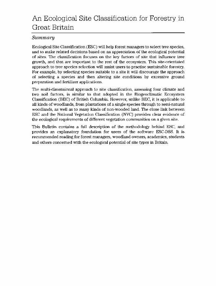
An Ecological Site Classification for Forestry in Great BritainSummary

Ecological Site Classification (ESC) will help forest managers to select tree species, and to make related decisions based on an appreciation o f the ecological potential o f sites. The classification focuses on the key factors o f site that influence tree growth, and that are important to the rest o f the ecosystem. This site-orientated approach to tree species selection will assist users to practise sustainable forestry. For example, by selecting species suitable to a site it will discourage the approach o f selecting a species and then altering site conditions by excessive ground preparation and fertilizer applications.

The multi-dimensional approach to site classification, assessing four climate and two soil factors, is similar to that adopted in the Biogeoclimatic Ecosystem Classification (BEC) o f British Columbia. However, unlike BEC, it is applicable to all kinds o f woodlands, from plantations o f a single species through to semi-natural woodlands, as well as to many kinds o f non-wooded land. The close link between ESC and the National Vegetation Classification (NVC) provides clear evidence o f the ecological requirements o f different vegetation communities on a given site.

This Bulletin contains a full description o f the methodology behind ESC, and provides an explanatory foundation for users o f the software ESC-DSS. It is recommended reading for forest managers, woodland owners, academics, students and others concerned with the ecological potential o f site types in Britain.

f

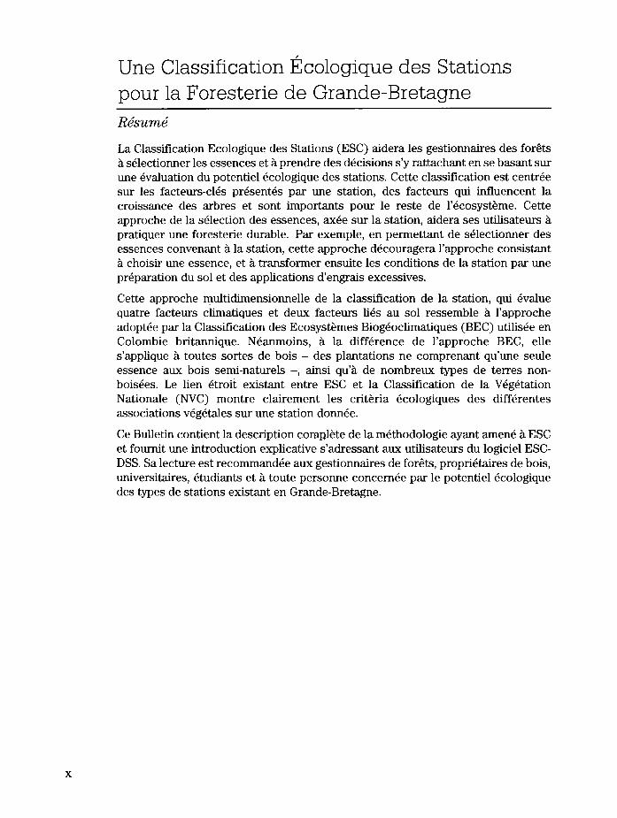
Une Classification Ecologique des Stations pour la Foresterie de Grande-BretagneResume

La Classification Ecologique des Stations (ESC) aidera les gestionnaires des forets a selectionner les essences et a prendre des decisions s’y rattachant en se basant sur une evaluation du potentiel ecologique des stations. Cette classification est centree sur les facteurs-cles presentes par une station, des facteurs qui influencent la croissance des arbres et sont importants pour le reste de l’ecosysteme. Cette approche de la selection des essences, axee sur la station, aidera ses utilisateurs a pratiquer une foresterie durable. Par exemple, en permettant de selectionner des essences convenant a la station, cette approche decouragera l’approche consistant a choisir une essence, et a transformer ensuite les conditions de la station par une preparation du sol et des applications d’engrais excessives.

Cette approche multidimensionnelle de la classification de la station, qui evalue quatre facteurs climatiques et deux facteurs lies au sol ressemble a l’approche adoptee par la Classification des Ecosystemes Biogeoclimatiques (BEC) utilisee en Colombie britannique. Neanmoins, a la difference de l ’approche BEC, elle s’applique a toutes sortes de bois - des plantations ne comprenant qu’une seule essence aux bois semi-naturels -, ainsi qu’a de nombreux types de terres non- boisees. Le lien etroit existant entre ESC et la Classification de la Vegetation Nationale (NVC) montre clairement les criteria ecologiques des differentes associations vegetales sur une station donnee.

Ce Bulletin contient la description complete de la methodologie ayant amene a ESC et foumit une introduction explicative s’adressant aux utilisateurs du logiciel ESC- DSS. Sa lecture est recommandee aux gestionnaires de forets, proprietaries de bois, universitaires, etudiants et a toute personne concemee par le potentiel ecologique des types de stations existant en Grande-Bretagne.

x

Okologische Standortklassifizierung fur die Forstwirtschaft in GroBbritannienZusammenfassung

Okologische Standortklassifizierung (ESC) hilft Forstmanagern, Baumarten auszuwahlen und damit verbundene Entscheidungen zu treffen, indem sie sich auf eine Bewertung des okologischen Potentials eines Standortes basiert. Die Klassifizierung konzentriert sich auf einige Schhisselfaktoren des Standortes, die den Baumwuchs beeinflussen und fiir das restliche Okosystem wichtig sind. Diese standort-bezogene Methode zur Baumartenwahl wird es dem Benutzer erleichtem, nachhaltige Forstwirtschaft zu betreiben. Durch die Auswahl von Arten die dem Standort angebracht sind, wird es zum Beispiel verhindert eine Art auszuwahlen und dann die Standortbedingungen durch iibermaSige Bodenbearbeitung und Diingeanwendung zu verandem.

Die multidimensionale Methode der Standortklassifizierung bewertet vier klimatische und zwei Bodenfaktoren und ahnelt damit der Biogeoklimatischen Okosystem Klassifizierung (BEC) von Britisch Kolumbien. Sie ist jedoch, im Gegensatz zu BEC, fur alle Waldarten, von Plantagen einer einzigen Art bis zu natumahen Waldem, aber auch fiir viele Arten von unbewaldetem Land anwendbar. Die enge Verbindung zwischen ESC und der Nationalen Vegetationsklassifizierung (NVC) liefert klare Beweise der okologischen Bediirfnisse verschiedener Vegetationsgemeinschaften an einem bestimmten Standort.

Dieses Bulletin enthalt eine voile Beschreibung der Methologie hinter ESC, und liefert eine Erklarungsgrundlage fur Benutzer des Computerprogrammes ESC-DSS. Es ist empfohlener Lesestoff fur Forstmanager, Waldbesitzer, Akademiker, Studenten und andere, die sich mit dem okologischem Potential der Standortarten in Britannien befassen.

Dosbarthiad Safleoedd Ecolegol ar gyfer Coedwigaeth ym Mhrydain Fawr

Crynodeb

Bydd Dosbarthiad Safleoedd Ecolegol (ESC) o gymorth i reolwyr coedwig er mwyn dewis rhywogaethau coed ac i wneud penderfyniadau sy’n gysylltiedig a hynny, penderfyniadau fyddai’n seiliedig ar werthfawrogiad o bosibiliadau ecolegol y safleoedd. Mae’r dosbarthu yn canolbwyntio ar ffactorau allweddol safleoedd sy’n dylanwadu ar dw f coed ac sy’n bwysig i weddill yr ecosystem. Bydd y dull hwn o gyfeirio at safleoedd wrth ddewis rhywogaethau coed yn cynorthwyo defnyddwyr i arfer coedwigaeth gynaliadwy. Er enghraifft, drwy ddewis rhywogaeth sy’n addas ar gyfer y safle, ni anogir y dull o ddethol rhywogaeth ac wedyn newid cyflwr y safle ar gyfer y rhywogaeth honno drwy orbaratoi’r ddaear a defnyddio gwrtaith yn ormodol.

Mae’r dull amlochrog tuag at ddosbarthu safleoedd, gan asesu pedwar ffactor hinsawdd a dau ffactor pridd, yn debyg i’r un a fabwysiadwyd yn Nosbarthiad Ecosystem Fioddaearhinsoddegol (BEC) Columbia Brydeinig. Fodd bynnag, yn wahanol i BEC, mae’n berthnasol i bob math o goetiroedd, o blanhigfeydd un rhywogaeth ymlaen i goetiroedd lled-naturiol, yn ogystal ag i lawer math o dir di- goed. Mae’r cyswllt agos rhwng ESC a’r Dosbarthiad Planhigion Cenedlaethol (NVC) yn rhoi tystiolaeth glir o anghenion ecolegol gwahanol gymunedau o blanhigion ar safle penodol.

Mae’r Bwletin hwn yn cynnwys disgrifiad llawn o ’r fethodoleg y tu ol i ESC, ac mae’n rhoi sail esboniadol ar gyfer defnyddwyr meddalwedd ESC-DSS. Anogir ei ddarllen gan reolwyr coedwig, perchnogion coetiroedd, academyddion, myfyrwyr ac eraill sy’n ymddiddori yn y posibiliadau ecolegol a geir mewn mathau o safleoedd ym Mhrydain.

Chapter 1

Introduction

This classification will help forest managers make decisions on silviculture and other aspects o f land use based on an appreciation o f the ecological potential o f sites. It is applicable to all kinds o f woodland, from plantations o f a single species through to semi-natural woodlands, and to many kinds o f non-wooded land. Ecological Site Classification (ESC) incorporates the existing classification o f forest soil types that has been the basis o f silviculture for many years (Pyatt, 1970, 1977). The new classification focuses on the key factors o f site that influence tree growth, and are important to the rest o f the ecosystem and its sustainable development. The new classification is therefore designed to support current forest policy (Forestry Commission, 1998).

ESC provides a method o f assessing site in a practical, cost-effective and, as far as is possible, quantitative way. The classification assumes that three principal factors determine site: climate, soil moisture regime and soil nutrient regime. The three factors can be thought o f as forming the axes o f a cube (Figure 1). For Britain as a whole the climate axis is divided into seven zones, and there are eight classes o f soil moisture regime and six classes o f soil nutrient regime. The combination o f moisture and nutrient regimes is referred to as soil quality, the grid formed from these axes being the soil quality grid. This three dimensional approach to site classification is similar to that adopted in the Biogeoclimatic Ecosystem Classification o f British Columbia (Pojar et al., 1987) and previously encouraged in Britain by Anderson (1950), Anderson and Fairbaim (1955) and Fairbaim (1960). Similar soil quality grids but with less formal climatic classifications are in widespread use in Europe (Ellenberg, 1988; Anon., 1991a and b; Rameau et al., 1989, 1993).

An individual site type, typically a homogeneous stand o f ground vegetation or patch o f soil with an area o f 10 m2 - 5 ha, will occupy one, or at most two cells o f the cube o f Figure 1. The site type will have a range o f soil quality encompassed by one class (or at most two adjacent classes) o f moisture and nutrient regime, within whichever climatic zone it lies. The classification contains a finite number o f site types, as represented by each cell within the cube o f Figure 1, that is 7 x 8 x 6 = 336. An individual forest will usually lie within one climatic zone and typically cover less than half of the soil quality grid, giving fewer than 24 site types. However, site types within one forest need not occupy contiguous cells, as there may be gaps in the coverage o f the grid.

Use o f the classification for an individual site involves three stages: the first is to identify the site type, the second is to consider the various silvicultural and ecological options possible for that site type, the third is to decide on the appropriate management o f the site in the light o f the objectives. ESC provides the means to accomplish the first step o f the process and the second step as far as choice o f species or native woodland type. In due course further ecological choices and other aspects o f site-related forest management will be added to the classification.

This Bulletin provides an explanatory and supporting framework for the Decision Support System (a compact disc with software referred to as the ESC Decision Support System or ESC-DSS; Forestry Commission, 2001), but does not attempt to duplicate its content. It provides a comprehensive description o f ESC but not a manual method for performing site analysis. Potential users o f ESC are encouraged to obtain an understanding o f the classification from this Bulletin and then explore the ESC-DSS.

Within the Bulletin, Chapters 2, 3 and 4 explain the basis for the classification o f the three principal components, climate, soil moisture regime and soil nutrient regime. Chapters 5 and 6 explain how indirect methods are used to evaluate soil quality. The final chapters 7 and 8 show how the site suitability o f individual tree species and types o f native woodland has been worked out, enabling land managers to make choices based on sound ecological principles.

This Bulletin and the ESC-DSS replace Technical Paper 20 (Pyatt and Suarez, 1997) and incorporate several major improvements to the system. The climate data are now available for the whole o f Britain and have been updated to the recording period 1961-90; a map o f windiness for the whole o f Britain has been prepared. Recent research has established the chemical basis o f soil nutrient regime and has provided a method o f assessing soil nutrient regime from the ground vegetation (Wilson, 1998).

In spite o f all this work ESC is not yet as good as we would like it to be. The prediction o f soil nutrient regime is based on too few sample plots to give adequate precision at the Very Poor end of the range, consequently the assessment o f such sites draws support from an earlier method (Taylor, 1991). The prediction o f the yield class likely to be achieved by tree species in pure stands is based on a method that is not yet validated. Further work is underway to extend the ecological and silvicultural choices provided by ESC site types, to develop a system linked to a Geographical Information System (GIS) and to improve the predictions o f soil nutrient regime and yield class. The application o f GIS and availability o f digital soil maps will be o f crucial importance to the effective use o f ESC at the forest scale. An example o f the benefits o f this approach to examine the potential effects o f different management strategies has been provided by the New Forest, Hampshire (Pyatt et al., 2001).

2

Chapter 2

Climate

Importance and choice of factorsClimate is important to foresters because it limits the means by which they can achieve their objectives o f management. Aspects o f climate constrain the variety o f tree species that can be planted, although in much o f Britain the choice is wide compared with many temperate areas. The climate, especially the available light and energy (warmth), sets an upper limit to the rate o f tree growth and timber yield. Equally, climate controls the other parts o f the forest ecosystem, whether they be biological, hydrological or pedological and sets the limits within which sustainable management can be practised.

Bio-climatic maps have previously been published for Scotland (Birse and Dry, 1970; Birse and Robertson, 1970; Birse, 1971) and for England and Wales (Bendelow and Hartnup, 1980). These maps, mostly at the 1:625 000 scale, are familiar to many foresters, but the small scale has limited their practical use to national or regional research studies. The climatic factors chosen for ESC are similar to those incorporated in these maps but are based on a larger set o f meteorological stations and modem methods o f interpolation.

Four climatic factors are currently used in ESC: ‘warmth’, ‘wetness’, ‘continentality’ and ‘windiness’. Warmth and wetness are the most important factors and are combined to define climatic zones o f relevance particularly to choice o f species. Continentality and windiness may refine species choice and the latter can have a major influence on timber production. All four factors are therefore required to describe the climatic conditions for tree growth at a site. A fifth climatic factor is under development (see the final section o f this chapter entitled ‘Winter cold, unseasonable frosts and other winter hazards’). Solar radiation in terms o f light level and duration

is vital for photosynthesis and therefore growth is dependent on factors such as latitude, aspect, slope and cloud cover. Evidence that solar radiation directly, rather than indirectly through temperature effects, limits tree growth in Britain is, however, lacking at present. The adjustments to accumulated temperature and soil moisture regime suggested in Tables 1 and 7 take account o f some o f the effects o f variation in solar radiation.

Except for windiness, the climatic factors have been calculated from data for the recording period 1961-90 supplied by the Meteorological Office, in most cases via the Climatic Research Unit (CRU) at the University o f East Anglia. The CRU dataset consists o f a number o f basic meteorological variables (monthly mean temperature, monthly rainfall, etc.) for each 10 x 10 km square throughout Britain (Barrow et al., 1993). Values for each climatic factor have been calculated for the 2836 squares, then the values have been interpolated to a finer resolution. The ESC-DSS supplies values for any 100 x 100 m grid reference in Britain. The climate maps included in this publication are mainly for illustration purposes and should not be used to read o ff a climatic value for a particular site. In order to reduce the map datasets to a manageable size, accuracy has been reduced.

WarmthIt is widely understood that summer or growing season warmth is a major determinant o f tree growth rate. For small areas o f the country relative warmth is conveniently approximated by elevation but at larger scales latitude and longitude are also necessary to predict warmth. Accumulated day-degrees above a ‘growth threshold’ temperature provide a convenient measure o f summer warmth. ESC follows a

3

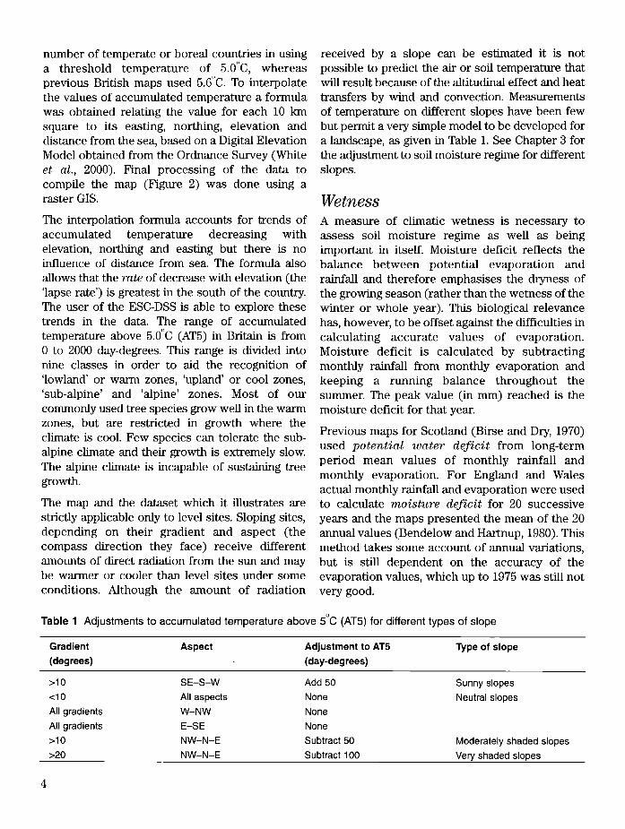
number o f temperate or boreal countries in using a threshold temperature o f 5.0"C, whereas previous British maps used 5.6 C. To interpolate the values o f accumulated temperature a formula was obtained relating the value for each 10 km square to its easting, northing, elevation and distance from the sea, based on a Digital Elevation Model obtained from the Ordnance Survey (White et al., 2000). Final processing o f the data to compile the map (Figure 2) was done using a raster GIS.

The interpolation formula accounts for trends of accumulated temperature decreasing with elevation, northing and easting but there is no influence o f distance from sea. The formula also allows that the rate o f decrease with elevation (the ‘lapse rate’) is greatest in the south o f the country. The user o f the ESC-DSS is able to explore these trends in the data. The range o f accumulated temperature above 5.0 C (AT5) in Britain is from 0 to 2000 day-degrees. This range is divided into nine classes in order to aid the recognition o f ‘lowland’ or warm zones, ‘upland’ or cool zones, ‘sub-alpine’ and ‘alpine’ zones. Most o f our commonly used tree species grow well in the warm zones, but are restricted in growth where the climate is cool. Few species can tolerate the sub- alpine climate and their growth is extremely slow. The alpine climate is incapable o f sustaining tree growth.

The map and the dataset which it illustrates are strictly applicable only to level sites. Sloping sites, depending on their gradient and aspect (the compass direction they face) receive different amounts o f direct radiation from the sun and may be warmer or cooler than level sites under some conditions. Although the amount o f radiation

received by a slope can be estimated it is not possible to predict the air or soil temperature that will result because o f the altitudinal effect and heat transfers by wind and convection. Measurements o f temperature on different slopes have been few but permit a very simple model to be developed for a landscape, as given in Table 1. See Chapter 3 for the adjustment to soil moisture regime for different slopes.

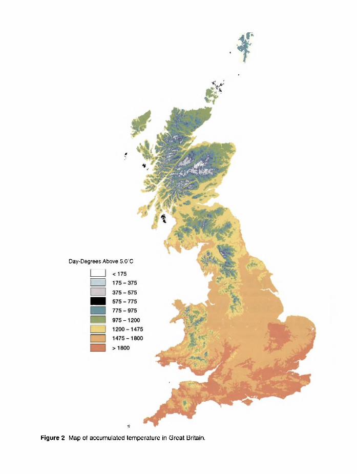
WetnessA measure o f climatic wetness is necessary to assess soil moisture regime as well as being important in itself. Moisture deficit reflects the balance between potential evaporation and rainfall and therefore emphasises the dryness o f the growing season (rather than the wetness o f the winter or whole year). This biological relevance has, however, to be offset against the difficulties in calculating accurate values o f evaporation. Moisture deficit is calculated by subtracting monthly rainfall from monthly evaporation and keeping a running balance throughout the summer. The peak value (in mm) reached is the moisture deficit for that year.

Previous maps for Scotland (Birse and Dry, 1970) used poten tia l water d e fic it from long-term period mean values o f monthly rainfall and monthly evaporation. For England and Wales actual monthly rainfall and evaporation were used to calculate m oisture deficit for 20 successive years and the maps presented the mean o f the 20 annual values (Bendelow and Hartnup, 1980). This method takes some account o f annual variations, but is still dependent on the accuracy o f the evaporation values, which up to 1975 was still not very good.

Table 1 Adjustments to accumulated temperature above 5°C (AT5) for different types of slope

Gradient(degrees)

Aspect Adjustment to AT5 (day-degrees)

Type of slope

>10 SE-S-W Add 50 Sunny slopes<10 All aspects None Neutral slopesAll gradients W -NW NoneAll gradients E-SE None>10 NW -N-E Subtract 50 Moderately shaded slopes>20 NW -N-E Subtract 100 Very shaded slopes

4

A

SA

CW

WW

CM

WM

WD

VD = Very Dry, MD = Moderately Dry, SD = Slightly Dry, F = Fresh, M = Moist, VM = Wet, VW = Very Wet.

VP = Very Poor, P = Poor, M = Medium, R = Rich, VR = Very Rich, C = Carbonate.

A = Alpine, SA = Sub-alpine, CW = Cool Wet, WW = Warm Wet, CM = Cool Moist, WM = Warm Moist, WD = Warm Dry.

Figure 1 The three ‘principal components’ of ecological site classification.

f

Figure 2 Map of accumulated temperature in Great Britain.

Millimetres

Figure 3 Map of moisture deficit in Great Britain.

43 '

DAMS score

Figure 4 Map of windiness (DAMS) in Great Britain.

f

Conrad Index

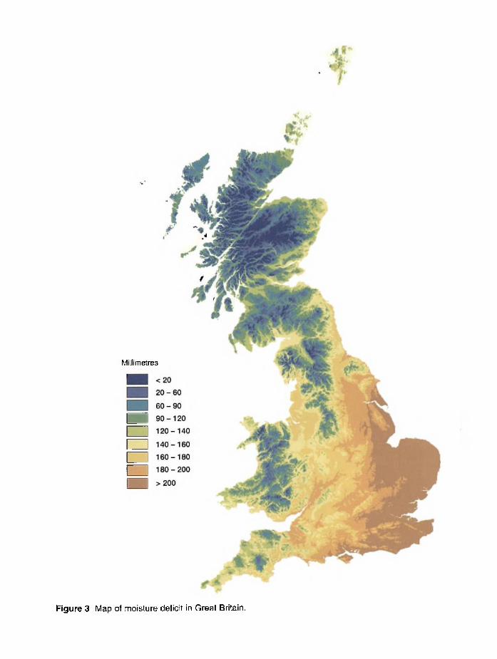
Figure 5 Map of continentality in Great Britain based on the Conrad index (reduced to sea level).

i l

*

Climate Zone

[ ____ ] Alpine

I | Sub-alpine

Cool Wet

Cool Moist

Warm Wet

Warm Moist

Warm Dry

Figure 6 Map of climatic zones in Great Britain based on accumulated temperature and moisture deficit.

Positive <------------------------ Planform > Negative

Contour line

Figure 7 Nine slope shapes combining profile and planform.

Forest soil types are listed in full in Appendix 4.

Figure 8 Simplified distribution of soil types and humus forms on the soil quality grid.

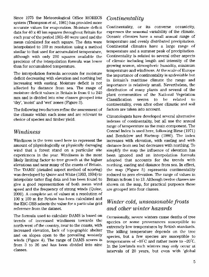
Since 1975 the Meteorological Office MORECS system (Thompson et al., 1981) has provided more accurate values for evaporation. Moisture deficit data for 40 x 40 km squares throughout Britain for each year o f the period 1961-90 were used and the mean calculated for each square. The data were interpolated to 100 m resolution using a method similar to that used for accumulated temperature, although with only 200 squares available the precision o f the interpolation formula was lower than for accumulated temperature.

The interpolation formula accounts for moisture deficit decreasing with elevation and northing but increasing with easting. Moisture deficit is not affected by distance from sea. The range o f moisture deficit values in Britain is from 0 to 240 mm and is divided into nine classes grouped into ‘dry’, ‘moist’ and ‘wet’ zones (Figure 3).

The following two factors refine the assessment o f the climate within each zone and are relevant to choice o f species and timber yield.

WindinessWindiness is the term used here to represent the amount o f physiologically or physically damaging wind that a forest stand on a particular site experiences in the year. Windiness is the most likely limiting factor to tree growth at the higher elevations and near many o f the coasts o f Britain. The ‘DAMS’ (detailed aspect method o f scoring) was developed by Quine and White (1993, 1994) to interpolate tatter flag data and has been found to give a good representation o f both mean wind speed and the frequency o f strong winds (Quine,2000). A complete set o f values at a resolution o f 100 x 100 m for Britain has been calculated and the ESC-DSS selects the value for a particular grid reference from the dataset.

The formula used to calculate DAMS is based on trends o f increased windiness towards the north-west o f the country, near to the coasts, with increased elevation, lack o f topographic shelter and on slopes open to the prevailing westerly winds (Figure 4). The range o f DAMS scores is from 3 to 36 and has been divided into nine classes.

ContinentalityContinentality, or its converse oceanicity, expresses the seasonal variability o f the climate. Oceanic climates have a small annual range of temperature and evenly distributed precipitation. Continental climates have a large range o f temperature and a summer peak o f precipitation. Continentality is related to several other aspects o f climate including length and intensity o f the growing season, atmospheric humidity, minimum temperature and windiness. At the scale o f Europe the importance o f continentality is undeniable but in Britain’s maritime climate the range and importance is relatively small. Nevertheless, the distribution o f many plants and severed o f the plant communities o f the National Vegetation Classification seems to be related to continentality, even after other climatic and soil factors are taken into account.

Climatologists have developed several alternative indexes o f continentality, but all use the annual range o f temperature as the main component. The Conrad Index is used here, following Birse (1971) and Bendelow and Hartnup (1980). The index increases with elevation, with easting and with distance from sea but decreases with northing. To simplify the map the influence o f elevation has been ignored and an interpolation formula adopted that accounts for the trends with northing, easting and distance from sea. In effect, the map (Figure 5) represents continentality reduced to zero elevation. The range o f values in Britain is from 1 to 13. Although twelve classes are shown on the map, for practical purposes these are grouped into four classes.

Winter cold, unseasonable frosts and other winter hazardsOccasionally, severe winters cause deaths o f tree species or some provenances susceptible to extremely low temperatures by British standards. The killing temperature depends on the tree species, but a few species are susceptible to temperatures o f -10 C and rather more to -20 C. In the lowlands such winters may only occur at intervals o f 20 years, but even with ‘global

5

warming’ there is reason to suppose that damaging winters w ill recur. Extreme temp­eratures normally occur during sustained periods o f cold weather in December, January or February. Serious damage to trees can be caused by much less extreme frosts if they occur outside the dormant season. Such ‘unseasonable frosts’ are unpredictable as to timing and may occur anywhere in the country but are more frequent in certain topographic conditions such as ‘frost hollows’.

It is not yet possible to provide a satisfactory map either o f extreme winter temperature or o f unseasonable frost for the requirements o f ESC. In the meantime, the ESC-DSS provides broad-brush advice on the use o f sensitive species such as rauli ( Nothofagus nervosa) and the Oregon and Washington origins o f Sitka spruce.

Heavy snow or ice storms occasionally cause breakage o f branches or even stems o f trees at any age. Although such events are unpredictable they

are more frequent in the north o f the country and at higher elevations. Certain races o f Scots pine and provenances o f lodgepole pine are particularly susceptible to snow damage, otherwise choice o f species does not appear to be constrained by this risk.

Climatic zonesThe four zones o f warmth and the three zones of wetness are combined (Table 2) to define seven climatic zones: Warm dry, Warm moist, Warm wet, Cool moist, Cool wet, Sub-alpine and Alpine (Figure 6). The climatic zones are useful for general descriptive purposes, e.g. for describing species suitability, although we may need to subdivide a zone for greater precision. For most practical interpretations, however, the precise values for each climatic factor as calculated using the ESC-DSS w ill be used directly, e.g. for predicting yield class, regardless o f the climatic zone the site is in.

Table 2 Definition of climatic zones in Great Britain by accumulated temperature and moisture deficit. (Shading indicates combinations not present)

Accumulated temperature (day-degrees above 5.0°C)

>1800 1800-1475

1475-1200

1200-975

975-775

775-575

575-375

375-175

<175

Moi

stur

e de

ficit

(mm

)

> 200

Warm Dry180-200

160-180

140-160

Warm Moist Cool Moist120-140

90-120

60-90 Warm Wet

Cool Wet20-60Sub-Alpine<20 Alpine

6

The area o f each c lim a tic zone is given in Table 3.

Table 3 Area of climatic zones in Great Britain

Zone Area (M ha) % of total

Alpine 0.12 0.5Sub-alpine 0.33 1.4Cool Wet 4.60 19.8Cool Moist 1.49 6.4Warm Wet 0.49 2.1Warm Moist 7.41 31.9Warm Dry 8.79 37.9

Total 23.23 100.0

The area o f individual sub-zones is shown in Table 4.

Table 4 Area of climatic sub-zones based on accumulated temperature and moisture deficit (km2). (Shading indicates combinations not present in Britain)

Accumulated temperature (day-degrees above 5.0°C)

>1800 1800-1475

1475-1200

1200-975

975-775

775-575

575-375

375-175

<175

>200 18142 14146

Ec 180-200 8221 16462

160-180 6459 23520 910

o 140-160 5180 15268 6470 78 449<D 120-140 1544 9388 13127 2917 762

90-120 48 3247 19835 10360 282 112 60-90 2 4896 17747 2554 18

20-60 2 5034 11676 885 <1

<20 2 1908 6175 3258 1012 223

7

Chapter 3

Soil moisture regime

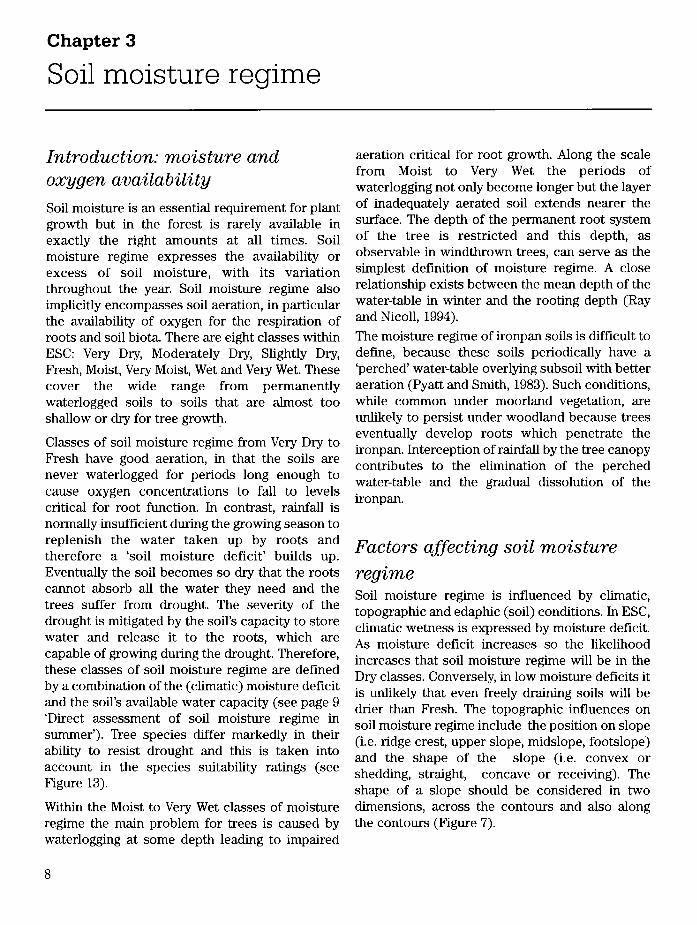
Introduction: moisture and oxygen availabilitySoil moisture is an essential requirement for plant growth but in the forest is rarely available in exactly the right amounts at all times. Soil moisture regime expresses the availability or excess o f soil moisture, with its variation throughout the year. Soil moisture regime also implicitly encompasses soil aeration, in particular the availability o f oxygen for the respiration o f roots and soil biota. There are eight classes within ESC: Very Dry, Moderately Dry, Slightly Dry, Fresh, Moist, Very Moist, Wet and Very Wet. These cover the wide range from permanently waterlogged soils to soils that are almost too shallow or dry for tree growth.

Classes o f soil moisture regime from Very Dry to Fresh have good aeration, in that the soils are never waterlogged for periods long enough to cause oxygen concentrations to fall to levels critical for root function. In contrast, rainfall is normally insufficient during the growing season to replenish the water taken up by roots and therefore a ‘soil moisture deficit’ builds up. Eventually the soil becomes so dry that the roots cannot absorb all the water they need and the trees suffer from drought. The severity o f the drought is mitigated by the soil’s capacity to store water and release it to the roots, which are capable o f growing during the drought. Therefore, these classes o f soil moisture regime are defined by a combination o f the (climatic) moisture deficit and the soil’s available water capacity (see page 9 ‘Direct assessment o f soil moisture regime in summer’). Tree species differ markedly in their ability to resist drought and this is taken into account in the species suitability ratings (see Figure 13).

Within the Moist to Very Wet classes o f moisture regime the main problem for trees is caused by waterlogging at some depth leading to impaired

aeration critical for root growth. Along the scale from Moist to Very Wet the periods o f waterlogging not only become longer but the layer o f inadequately aerated soil extends nearer the surface. The depth o f the permanent root system o f the tree is restricted and this depth, as observable in windthrown trees, can serve as the simplest definition o f moisture regime. A close relationship exists between the mean depth o f the water-table in winter and the rooting depth (Ray and Nicoll, 1994).

The moisture regime o f ironpan soils is difficult to define, because these soils periodically have a ‘perched’ water-table overlying subsoil with better aeration (Pyatt and Smith, 1983). Such conditions, while common under moorland vegetation, are unlikely to persist under woodland because trees eventually develop roots which penetrate the ironpan. Interception o f rainfall by the tree canopy contributes to the elimination o f the perched water-table and the gradual dissolution o f the ironpan.

Factors affecting soil moisture

regimeSoil moisture regime is influenced by climatic, topographic and edaphic (soil) conditions. In ESC, climatic wetness is expressed by moisture deficit. As moisture deficit increases so the likelihood increases that soil moisture regime will be in the Dry classes. Conversely, in low moisture deficits it is unlikely that even freely draining soils will be drier than Fresh. The topographic influences on soil moisture regime include the position on slope (i.e. ridge crest, upper slope, midslope, footslope) and the shape o f the slope (i.e. convex or shedding, straight, concave or receiving). The shape o f a slope should be considered in two dimensions, across the contours and also along the contours (Figure 7).

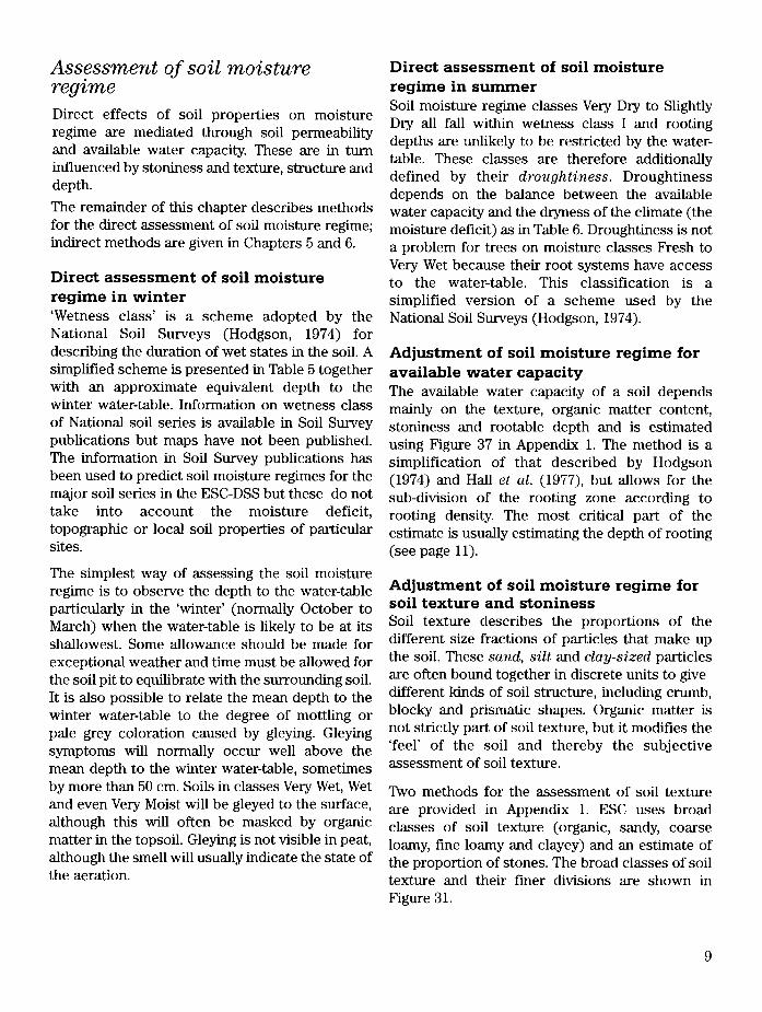
Assessment of soil moisture regimeDirect effects o f soil properties on moisture regime are mediated through soil permeability and available water capacity. These are in turn influenced by stoniness and texture, structure and depth.

The remainder o f this chapter describes methods for the direct assessment o f soil moisture regime; indirect methods are given in Chapters 5 and 6.

Direct assessment of soil moisture regime in winter‘Wetness class’ is a scheme adopted by the National Soil Surveys (Hodgson, 1974) for describing the duration o f wet states in the soil. A simplified scheme is presented in Table 5 together with an approximate equivalent depth to the winter water-table. Information on wetness class o f National soil series is available in Soil Survey publications but maps have not been published. The information in Soil Survey publications has been used to predict soil moisture regimes for the major soil series in the ESC-DSS but these do not take into account the moisture deficit, topographic or local soil properties o f particular sites.

The simplest way o f assessing the soil moisture regime is to observe the depth to the water-table particularly in the ‘winter’ (normally October to March) when the water-table is likely to be at its shallowest. Some allowance should be made for exceptional weather and time must be allowed for the soil pit to equilibrate with the surrounding soil. It is also possible to relate the mean depth to the winter water-table to the degree o f mottling or pale grey coloration caused by gleying. Gleying symptoms will normally occur well above the mean depth to the winter water-table, sometimes by more than 50 cm. Soils in classes Very Wet, Wet and even Very Moist will be gleyed to the surface, although this will often be masked by organic matter in the topsoil. Gleying is not visible in peat, although the smell will usually indicate the state of the aeration.

Direct assessment of soil moisture regime in summerSoil moisture regime classes Very Dry to Slightly Dry all fall within wetness class I and rooting depths are unlikely to be restricted by the water- table. These classes are therefore additionally defined by their droughtiness. Droughtiness depends on the balance between the available water capacity and the dryness o f the climate (the moisture deficit) as in Table 6. Droughtiness is not a problem for trees on moisture classes Fresh to Very Wet because their root systems have access to the water-table. This classification is a simplified version o f a scheme used by the National Soil Surveys (Hodgson, 1974).

Adjustment of soil moisture regime for available water capacityThe available water capacity o f a soil depends mainly on the texture, organic matter content, stoniness and rootable depth and is estimated using Figure 37 in Appendix 1. The method is a simplification o f that described by Hodgson (1974) and Hall et al. (1977), but allows for the sub-division o f the rooting zone according to rooting density. The most critical part o f the estimate is usually estimating the depth o f rooting (see page 11).

Adjustment of soil moisture regime for soil texture and stoninessSoil texture describes the proportions o f the different size fractions o f particles that make up the soil. These sand, s ilt and clay-sized particles are often bound together in discrete units to give different kinds o f soil structure, including crumb, blocky and prismatic shapes. Organic matter is not strictly part o f soil texture, but it modifies the ‘fee l’ o f the soil and thereby the subjective assessment o f soil texture.

Two methods for the assessment o f soil texture are provided in Appendix 1. ESC uses broad classes o f soil texture (organic, sandy, coarse loamy, fine loamy and clayey) and an estimate o f the proportion o f stones. The broad classes o f soil texture and their finer divisions are shown in Figure 31.

9

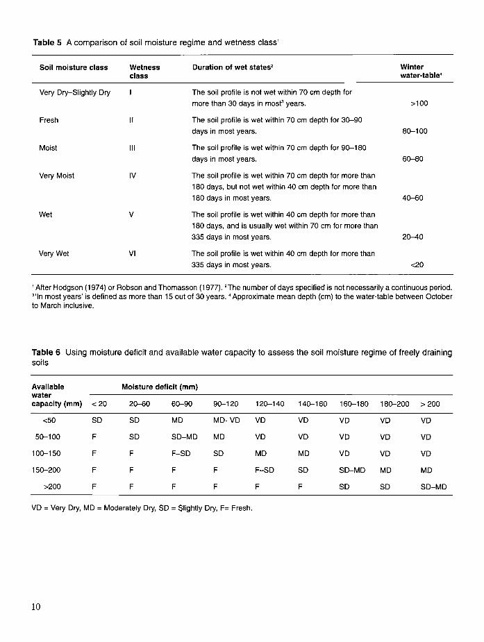
Table 5 A comparison of soil moisture regime and wetness class'

Soil moisture class Wetnessclass

Duration of wet states2 Winterwater-table4

Very Dry—Slightly Dry 1 The soil profile is not wet within 70 cm depth for more than 30 days in most3 years. >100

Fresh II The soil profile is wet within 70 cm depth for 30-90 days in most years. 80-100

Moist III The soil profile is wet within 70 cm depth for 90-180 days in most years. 60-80

Very Moist IV The soil profile is wet within 70 cm depth for more than 180 days, but not wet within 40 cm depth for more than 180 days in most years. 40-60

Wet V The soil profile is wet within 40 cm depth for more than 180 days, and is usually wet within 70 cm for more than 335 days in most years. 20-40

Very Wet VI The soil profile is wet within 40 cm depth for more than 335 days in most years. <20

' After Hodgson (1974) or Robson and Thomasson (1977). 2The number of days specified is not necessarily a continuous period. 3'In most years' is defined as more than 15 out of 30 years. * Approximate mean depth (cm) to the water-table between October to March inclusive.

Table 6 Using moisture deficit and available water capacity to assess the soil moisture regime of freely draining soils

Availablewatercapacity (mm)

Moisture deficit (mm)

< 20 20-60 60-90 90-120 120-140 140-160 160-180 180-200 > 200

<50 SD SD MD MD- VD VD VD VD VD VD

50-100 F SD SD-MD MD VD VD VD VD VD

100-150 F F F-SD SD MD MD VD VD VD

150-200 F F F F F-SD SD SD-MD MD MD

>200 F F F F F F SD SD SD-MD

VD = Very Dry, MD = Moderately Dry, SD = Slightly Dry, F= Fresh.

10

Adjustment of soil moisture regime for rooting depthEstimating rooting depth is often difficult but nevertheless important. Opportunity may be provided by windthrown trees to build up a direct local conversion from soil type to rooting depth. Only by this kind o f observation is it possible to be sure, for example, that, even without cultivation, roots can penetrate an ironpan or a compact or very stony subsoil layer or how far roots penetrate horizons with gleying symptoms. In freely draining soils that are not underlain by hard bedrock it is difficult to observe rooting depth because trees are rarely windthrown. In such circumstances, especially in lowland Britain where moisture deficits are large, it is reasonable to assume that the rooting depth is 1-1.5 m. On sandy soils a figure o f 2 m would be appropriate. The zone from which a tree is able to take up moisture will always exceed the depth o f roots or attached soil lifted out when the tree is uprooted.

The water-holding capacity o f organic material is so high that it is important to do a separate calculation for the humus layer whenever it is thicker than a few centimetres.

Adjustment of soil moisture regime for aspect and slopeSlopes facing the sun are drier (and warmer) than shaded slopes and this is expressed in soil development. Brown earths extend to higher elevation on sunny slopes than shaded slopes and, conversely, ironpan soils occur to lower elevations on shaded slopes than on sunny slopes. Detailed data on soil moisture differences on different slopes are few, so the following are practical approximations. Table 7 defines ‘sunny’, ‘shaded’ and ‘neutral’ slopes and provides final adjustments for soil moisture regime classes Very Dry, Moderately Dry, Slightly Dry, Fresh and Moist (as determined by available water capacity and moisture deficit). Wetter classes do not need adjustment.

Table 7 Adjustments to soil moisture regime for different types of slope

Gradient (degrees) Aspect Adjustment to SMR Type of slope

>10 SE-S-W A half class drier Sunny slopes<10 All aspects None Neutral slopes

All gradients W -NW NoneAll gradients E-SE None>10 NW -N-E A half class moister Moderately shaded slopes>20 NW -N-E One class moister Very shaded slopes

11

Chapter 4

Soil nutrient regime

Introduction: nutrient availabilitySoil nutrient regime expresses the availability o f soil nutrients for plant growth. The most important soil nutrients are nitrogen (N ), phosphorus (P), potassium (K), calcium (Ca) and magnesium (Mg). Other elements, including sulphur (S ) and those often referred to as ‘micronutrients’ that are needed in smaller quantities, are rarely deficient in British forest soils (Binns et al., 1980). The acidity (measured as pH) o f the soil is also important as the solubility and availability for plant uptake o f most nutrients is dependent upon the acidity o f the soil water. In ESC the gradient o f soil nutrient regime is arbitrarily divided into six classes: Very Poor, Poor, Medium, Rich, Very Rich and Carbonate.

Nitrogen is mainly taken up by plants in so-called mineral form, either as ammonium (NH.,) or nitrate (N 0 3) ions, although recent research suggests that some plants can also take up amino acids. Most plants seem to take up both forms o f mineral N but some plants have a preference for soils that supply most o f the N in either the NH, or NO:j form. There are relatively few examples o f plants that prefer NH.,-nitrogen, including several ericaceous species, whereas those that prefer NO:rnitrogen, the so-called nitrophiles, include many o f the species found on Very Rich soil nutrient regimes (Ellenberg, 1988, p. 129). Strongly acid soils, including many peats, tend to provide mineral N in the NH., form only, because the nitrification process whereby NH,-nitrogen is converted to N 03-nitrogen is blocked. At the other extreme, in Very Rich soils, NH.,-nitrogen released from the decomposition o f organic matter is rapidly nitrified and most o f the mineral N exists in the N 03 form (Wilson, 1998).

Factors affecting nutrient availability and their potential modificationIt is possible for soils to have adequate quantities o f all nutrient elements except one or two. In Britain P is the element most likely to be deficient, especially in very sandy or peaty soils. It has often been necessary to ‘prime’ the soil with an application o f P in order for tree growth to reflect properly the availability o f the other nutrients and permit productive forestry (Taylor, 1991). The application o f P fertilizer dramatically improves the soil nutrient regime and has a long-term effect. Such modifications may not be necessary when re-creating native woodlands.

The supply o f N varies greatly in British forest soils. At one extreme the lack o f N can be the main limiting factor in the soil, as in some podzolic or raw sandy soils with little organic matter. Nitrogen fertilizer can be applied to such soils but the effect may last only three years. Many strongly acid, peaty soils contain a large quantity o f N but only a small proportion is available for uptake. The availability o f the N in the peat can be enhanced by increasing the pH or the P supply. Increasing the pH is a difficult and expensive process and is rarely attempted, whereas the application o f P to such peats is commonplace. The availability o f N on infertile soils is often complicated by the presence o f competitive weeds o f the ericaceous family, especially heather and usually improves when such weeds are controlled or shaded out (Taylor and Tabbush, 1990).

On the deeper peat soils K may be in short supply. This tends to be linked to certain underlying lithologies and to areas well away from the influence o f the sea. Elements that are supplied in

12

significant quantities in precipitation include sodium, chlorine, K, Ca, Mg and N, but (importantly) not P. K deficiency in peaty soils is normally dealt with at the same time as P deficiency through the application o f PK fertilizer.

Some acid siliceous soils have only small quantities o f Ca or Mg. Concerns have been raised about the long-term supplies o f these elements but to date there have not been any problems in forest stands.

It is also possible for soils to have excessive quantities o f one nutrient, thereby impairing the uptake o f one or more others. An example might be Ca in shallow soils derived from chalk, where the pH o f the topsoil is over 7.5. Such soils, falling within the definition o f the Carbonate class o f nutrient regime, tend to have problems o f plant uptake o f P, N, K and some o f the micronutrients. It is not possible to cure all o f the nutrient problems o f these soils and the best solution is either to plant one o f the few tolerant tree species or to leave such sites unplanted. Another example o f an excessive nutrient supply is given by the soils developed directly on serpentine rocks rich in Mg, but these are rare in Britain.

Wilson et al. (1998) showed that the most important variables in soil nutrient regime are soil pH and N 0 3-nitrogen. The other major nutrients, Ca, Mg, K and P generally increase from the Very Poor class to the Very Rich class, but not necessarily at the same rate. Thus within any one class o f soil nutrient regime, e.g. Medium, it is possible to have soils with relatively high levels o f pH or o f two or three nutrients and relatively low levels o f the others. The work also showed that NH4-nitrogen, the total amount o f nitrogen (including organic forms) or the quantity o f organic matter itself were not strongly involved in soil nutrient regime as a whole. It is possible, however, that the importance o f NH.rnitrogen in

very acid soils may be under-estimated, because Wilson et al. (1998) sampled few such soils. The Carbonate class o f soils was not sampled at all, hence our knowledge o f this class is based on previous work, e.g. Wood and Nimmo (1962).

Assessment of soil nutrient regimeThe remainder o f this chapter describes methods for the direct assessment o f soil nutrient regime; indirect methods are given in Chapters 5 and 6.

Direct assessment of soil nutrient regimeDirect assessment o f nutrient regime requires multiple core sampling o f the soil to a depth o f at least 25 cm. The amount o f work involved would normally only be justified for research purposes.

The main properties o f the six classes are given in Table 8. The pH o f the soil is most useful for distinguishing the Carbonate, Very Rich and, to a lesser extent, the Rich class from the others. The Very Poor, Poor and Medium classes show little difference in their pH ranges. For the individual nutrients, there is a great deal o f overlap between adjacent classes in the quantities recorded, therefore only qualitative descriptions o f the classes are given. The importance o f N and (in the poorer classes) P is emphasised in Table 8.

The broad link between soil types, lithology, humus forms and soil nutrient regime is discussed in Chapter 5. The effectiveness with which ground vegetation can be used to predict soil nutrient regime without the need for soil chemical analysis is dealt with in Chapter 6.

13

Table 8 Some chemical properties of soil nutrient classes in relation to silviculture

Soil nutrient regimeVery Poor Poor Medium Rich Very Rich Carbonate

pH (HaO) in upper 25 cm depth

3.0—4.0 3.0—4.0 3.0-5.0 3.0-5.5 4.5-7.5 7.5-8.5

P availability low moderate to high

usually high high very high low to moderate

P fertilizer requirement*

E. likely R. possible

E. likely except for pines,R. unlikely

unlikely except for basic igneous and some shale lithologies

unlikely none uncertain

N availability very low, mainly NH4 with a littlen o 3

low, mainly NH4 with some N 03

moderate, both NH4 and N 03

moderate to high, both NH4 and NOa

very high, mainly NOa

moderate, mainly N 03

N category' D, C , some B

B, A A not applicable not applicable not applicable

N fertilizer requirement*

E. and R. likely for species other than

pines and larches

E. and R. possible for species other than pines and larches

unlikely none none uncertain

Other nutrient problems

K often deficient

on peats

none likely none likely none likely none likely N,P,K and micro­nutrients (Fe, Mn) can

be unavailable

* E. for woodland establishment on bare land. * R. restocking existing woodlands. # where Calluna present (from Taylor, 1991).

14

Chapter 5

Indirect assessment of soil moisture and nutrient regimes from soil type, lithology and humus form

Introduction: forest soil types and nutrient regimeSoil type gives an initial indication o f the ecological potential o f the site. Figure 8 shows an arrangement o f the main forest soil types (see Appendix 4) on the soil quality grid, but is a simplification and only the first step in a process o f prediction o f soil moisture and nutrient regimes. In this chapter the relationships between soil type, lithology, humus form and soil quality are explored in more detail.

In Figure 8 the soil types are shown rather precisely in terms o f soil moisture regime. In practice there will be overlap between the soil types, for example as a consequence o f the improvement o f bare land by drainage. Typically this will lift peats, peaty gleys and surface-water gleys up the scale by one-half to a full class. Ironpan soils likewise move up at least one class when woodland conditions are established. At the drier end o f the range, Figure 8 does not allow for the full ranges o f moisture deficit and available water capacity.

The spread o f soil nutrient regime within soil groups is larger than shown in Figure 8. Brown earths, surface-water gleys and peaty gleys, when bare land as well as wooded sites are included, range from Very Poor to Very Rich. Podzols are usually Very Poor or Poor but a few fall into Medium. Deep peats also have a skewed distribution towards the Very Poor end o f the range but examples in Rich or Very Rich seem to exist (none were sampled by Wilson, 1998). Ironpan soils are the least variable group, being restricted to Very Poor and Poor. Rendzinas, in the strict sense o f being shallow and strongly

calcareous, are the defining soils o f the Carbonate class, but deeper and less calcareous soils seem to be invariably Very Rich.

Clearfelling a woodland often leads to a temporary ‘flush’ o f nutrients due to an increased rate o f decomposition o f the humus and leaf litter (Adamson et al., 1987). The regrowth o f vegetation is more vigorous and contains species usually associated with more fertile conditions than were present before (see Chapter 6).

In ESC-DSS a prediction o f soil moisture and nutrient regimes is provided for three alternative classifications o f soil types (Forestry Commission, Soil Survey o f Scotland, Soil Survey o f England & Wales) in order to cater for the varying availability o f maps in different parts o f the country. The forest soil classification as presented in Appendix 4 is best suited for use in ESC (see also Kennedy,2001). The 1:50 000 or 1:25 000 scale maps o f the Soil Survey o f England & Wales and the Soil Survey o f Scotland provide a classification at the level o f soil series and are useful within their limitations o f scale. Such maps exist throughout lowland Scotland, for large parts o f Wales, but have only a scattered distribution in England. The national coverage o f maps at the scale o f 1:250 000 provides a classification o f ‘soil associations’, each o f which may comprise a mosaic o f disparate soil series and is usually more informative about the lithology than the soil type. The predicted moisture and nutrient regimes based on soil associations are not adequate for forest management purposes, but should be supplemented with local observations. The detailed discussion that follows is therefore confined to the forest soil types.

15

Local adjustment of soil moisture regime derived from soil typeForest soil type is more reliable for predicting soil moisture for the classes Moist to Very Wet than it is for Fresh to Very Dry. For the latter a direct assessment via available water capacity and moisture deficit is required (see Chapter 3). On a local (forest) scale the differences in moisture regime between any o f the soil types shown in Figure 8 may need to be shifted up or down by half a class. This reflects that, on the national scale, soil types have overlapping ranges o f moisture regime.

There is an interaction between moisture and nutrient regimes, such that the driest classes are rarely richer than Medium, and the wettest sites are rarely Very Rich.

Local adjustment of soil nutrient regime derived from soil typeInadequate sampling o f sites in the Very Poor class o f nutrient regime results in a lack o f precision in ESC in recognising soils within this class. Until more research can be undertaken it is useful to classify sites with some cover o f heather ( Calluna vulgaris) using the method devised by Taylor (1991). This recognised four categories o f nitrogen availability (fuller details are given in Appendix 6):

Category A: Sufficient N available foracceptable tree growth

Category B: N in short supply due tocompetition from heather

Category C: N in short supply due to slowmineralisation and competition from heather

Category D: N in short supply due to very slowmineralisation.

It is now clear that some o f the variation in nutrient regime within soil types is related to the lithology o f the parent material. There is no simple or precise way o f describing that relationship because o f the variability w ith in geological strata. However, a broad grouping o f lithologies helps to refine the relationship between soil type and nutrient regime. A previous grouping for nitrogen availability has been slightly modified and extended to cover lowland England (Table 9).

The procedure for recognising the nitrogen availability category involves identifying the forest soil type (Appendix 4) in Table 10 (page 18) and the nitrogen availability categories listed alongside. Where more than one category is listed, the appropriate lithology group is found in Table 9. Group I lithologies require a move o f two nitrogen availability categories to the right (e.g. from A to C for soil type 4); within Group II, move one category to the right (e.g. from C to D for soil type lib ); within Group III no amendment is required. In addition, if the soil type is mineral or organo- mineral (soil group codes 1, 3, 4, 6 or 7 in Table 10) and the site is dominated by heather (more than 50% ground cover - equivalent to the ‘ericaceous phase’ mapped in Forestry Commission soil surveys) move one further category to the right. The additional step should not be applied if the soil is classified as deep peat, i.e. soil group codes 8, 9 10 or 11. When recently fire-damaged vegetation is encountered, the dominance rating given to heather will need to be adjusted to that apparent locally on the same site type where there has been enclosure and protection from fire.

The final step in assessing nutrient regime o f the poorer soils is to interpret the nitrogen availability category in terms o f the classes o f soil nutrient regime using Table 11.

16

Table 9 Ranking of the main lithologies according to the likely availability of nitrogen in overlying soils (based onTaylor, 1991)

Group 1 Low nitrogen availability Geological map* formation numbersTorridonian sandstone 61Moine quartz-feldspar-granulite, quartzite and granitic gneiss 8, 9, 10, 12Cambrian quartzite 62Dalradian quartzites 17Lewisian gneiss 1Quartzose granites and granulites 34 (part only)Acid volcanic and intrusive rocks 41, 46, 47Middle/Upper Old Red Sandstone (Scotland) 77, 78Upper Jurassic sandstones and grits 97, 98, 99Carboniferous grits and sandstones 81 (part only)

Group II Moderate nitrogen availabilityMoine mica schists and semi-pelitic schists 11Dalradian quartzose and mica schists, slates and phyllites 18, 19, 20, 21, 23Granites (high feldspar, low quartz content) 34 (part only)Tertiary basalts 57Old Red Sandstone basalts, andesite and tuff 44, 48, 50Silurian/Ordovician greywackes, mudstones (Scotland) 70, 71, 72, 73, 74Lower and Middle Jurassic sediments 91, 94, 95Hastings Beds 102

Tertiary sands and gravels 109

Group III High nitrogen availabilityGabbro, dolerite, epidiorite and hornblende schist 14, 15, 26, 27, 32, 33, 35

Lower Old Red Sandstone 75

New Red Sandstone 85, 89, 90

Cretaceous shales 102-106 (part only)

Tertiary clays 107-111 (part only)

Upper and Lower greensands 104, 105

Carboniferous shales and basalts Silurian/Ordovician/Devonian shales

53, 54, 80*, 81 (part only) 82, 83, 84

(Wales and south-west England) 68, 69, 70, 71, 72, 73, 74, 75, 76, 77, 78

Limestones and chalk 24, 67, 80*. 86, 91-101, 106

Cambrian/Precambrian 60, 64, 65, 66

* Reference: British Geological Survey, Geological Survey Ten Mile Map (3rd Edition Solid, 1979), published by the Ordnance Survey;

t refers to Scotland only;

t refers to England and Wales only

Notes:

1. Geological Map formation no. 34 has been subdivided into: (a) quartzose granites and granulites (Group I), (b) granites with a high feldspar and low quartz content (Group II).

2. Geological Map formation no. 81 has been subdivided into: (a) grits and sandstones (Group I), (b) shales (Group III).

3. Where soils occur over drift material, then their characteristics (in terms of nitrogen availability) will be similar to that of the solid rock from which the drift was derived.

17

Table 10 Main forest soil types categorised by nitrogen availability (based on Taylor, 1991)

Soil group Code Soil type Category

Brown earths 1 Typical brown earth A1d Basic brown earth A1u Upland brown earth A B1 z Podzolic brown earth A B1e Ericaceous brown earth A B C

Podzols 3 Typical podzol B C D3m Hardpan podzol B C D

3p Peaty podzol B C

Ironpan soils 4b Intergrade ironpan soil A B C4 Ironpan soil A B C D4z Podzolic ironpan soil B C D

4p Peaty ironpan soil A B C

Peaty gley soils 6 Peaty gley A B C D6z Peaty podzolic gley B C

Surface-water gley soils 7 Surface-water gley A B C7b Brown gley A7z Podzolic gley A B C

Basin bogs 8a Phragmites bog A8b Juncus articulatus or acutiflorus bog A8c Juncus effusus bog A8d Carex bog A

Flushed blanket bogs 9a Molinia, Myrica, Salix bog A9b Tussocky Molinia bog; Molinia, Calluna bog A B9c Tussocky Molinia, Eriophorum vaginatum B C

bog9d Non-tussocky Molinia, Eriophorum B C

vaginatum, Trichophorum bog9e Trichophorum, Calluna, Eriophorum, B C D

Molinia bog (weakly flushed)

Sphagnum bogs 10a Lowland Sphagnum bog D10b Upland Sphagnum bog D

Unflushed blanket bogs 11a Calluna blanket bog c D11b Calluna, Eriophorum vaginatum blanket bog c D11c Trichophorum, Calluna blanket bog D11 d Eriophorum blanket bog D

18

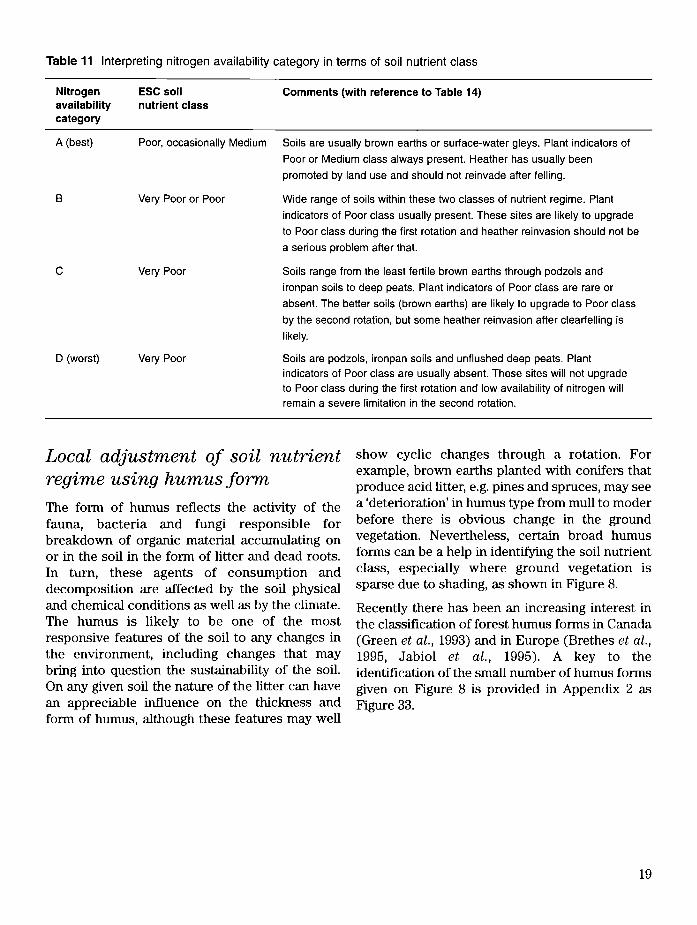
Table 11 Interpreting nitrogen availability category in terms of soil nutrient class

Nitrogenavailabilitycategory

ESC soil nutrient class

Comments (with reference to Table 14)

A (best)

D (worst)

Poor, occasionally Medium

Very Poor or Poor

Very Poor

Very Poor

Soils are usually brown earths or surface-water gleys. Plant indicators of Poor or Medium class always present. Heather has usually been promoted by land use and should not reinvade after felling.

Wide range of soils within these two classes of nutrient regime. Plant indicators of Poor class usually present. These sites are likely to upgrade to Poor class during the first rotation and heather reinvasion should not be a serious problem after that.

Soils range from the least fertile brown earths through podzols and ironpan soils to deep peats. Plant indicators of Poor class are rare or absent. The better soils (brown earths) are likely to upgrade to Poor class by the second rotation, but some heather reinvasion after clearfelling is likely.

Soils are podzols, ironpan soils and unflushed deep peats. Plant indicators of Poor class are usually absent. These sites will not upgrade to Poor class during the first rotation and low availability of nitrogen will remain a severe limitation in the second rotation.

Local adjustment of soil nutrient regime using humus formThe form o f humus reflects the activity o f the fauna, bacteria and fungi responsible for breakdown o f organic material accumulating on or in the soil in the form o f litter and dead roots. In turn, these agents o f consumption and decomposition are affected by the soil physical and chemical conditions as well as by the climate. The humus is likely to be one o f the most responsive features o f the soil to any changes in the environment, including changes that may bring into question the sustainability o f the soil. On any given soil the nature o f the litter can have an appreciable influence on the thickness and form o f humus, although these features may well

show cyclic changes through a rotation. For example, brown earths planted with conifers that produce acid litter, e.g. pines and spruces, may see a ‘deterioration’ in humus type from mull to moder before there is obvious change in the ground vegetation. Nevertheless, certain broad humus forms can be a help in identifying the soil nutrient class, especially where ground vegetation is sparse due to shading, as shown in Figure 8.

Recently there has been an increasing interest in the classification o f forest humus forms in Canada (Green et al., 1993) and in Europe (Brethes et al., 1995, Jabiol et al., 1995). A key to the identification o f the small number o f humus forms given on Figure 8 is provided in Appendix 2 as Figure 33.

19

Chapter 6

Indirect assessment of soil moisture and nutrient regimes from indicator plants

Introduction: the use of indicator plants in forestryPlants have a certain range o f tolerance o f soil moisture, pH, nitrate-nitrogen, as well as temperature, light and so on. This is referred to as their ecological amplitude on each scale. When growing with other plants in a community they will usually exhibit a narrower amplitude within which they can compete successfully, their ‘ecological niche’. I f we know the ecological preferences for the plants in a community we can make inferences about the ecological conditions at the site.

The ecological amplitude o f plants is variable. Clearly, those with a smaller amplitude (e.g. dog’s mercury or wavy hair-grass) are better indicators o f soil quality than those with a larger amplitude (e.g. bracken or rose-bay willowherb). Because most (and probably all) plants have an ecological niche wider than one class o f soil moisture or nutrient regime it follows that plants from several classes may be found growing together at any particular site. This does not invalidate the method but it does imply that only the community o f plants properly reflects soil quality. Indeed, Wilson (1998) showed that a detailed quantitative assessment o f the vegetation provides a reliable indication o f ESC soil nutrient class (together with a less precise indication o f soil moisture).

The use o f indicator plants in British forestry goes back to Gilchrist (1872) who recognised that ground vegetation indicated soil suitable for planting certain trees. In Europe, Cajander (1926) used groups o f plants to help identify forest types in terms o f soil moisture and nutrients, but thought o f these as confounded, i.e. a single axis from dry/very poor to wet/very rich. Anderson (1950) seems to have been the first to use a grid o f soil moisture and nutrient classes to help describe site types in terms o f a few plants. Ellenberg

(1988) used larger groups o f plants to defme locations on a soil moisture-pH grid. In British Columbia, Klinka et al. (1989) used lists o f plants to identify classes o f soil moisture and nutrient regime and described the ecological conditions in which individual species occurred. Indicator plant groups are used to describe site types on a soil moisture/nutrient grid as an aid to tree species choice in Belgium (Anon., 1991a and b). More recently in Britain, Rodwell and Patterson (1994) have listed ‘optimal precursor’ plants indicative o f ground suitable for creation o f particular new native woodland communities.

The use of numerical indicator valuesEllenberg (1988) provided indicator values, in integers from 1 to 9, to describe the soil preferences o f vascular plants (flowering plants and ferns) in terms o f three factors. The F value is related to soil moisture, the R value is related to soil reaction or base-status and the N value is related to nutrient supply, especially nitrogen. An F, R or N value o f 1 indicates a preference for, or at least a tolerance of, very low amounts, i.e. very dry, very acid or very nutrient-poor soil. A value o f 9 indicates a preference for very wet, strongly calcareous or very nutrient-rich soil. Ellenberg et al. (1992) extended the list o f values from vascular plants to bryophytes and lichens. Ellenberg values are available for over 1000 British plants, but the applicability o f values assigned subjectively on the basis o f the behaviour o f the plants in Central Europe is not assured. There are also many missing values, either where Ellenberg could not assign a value or where the plant was considered to show no ecological preference. As a consequence further work has been carried out.

Indicator values directly related to ESC soil nutrient regime have been objectively derived for

20

about 85 vascular plants growing in British woodlands (Wilson, 1998). Wilson’s indicator values are based on combining vegetation and soil chemical data and are preferable to subjectively assigned values. However, the reliability o f the Wilson value depends on the frequency with which the species occurred in Wilson’s sample plots, and the values for only 52 species are considered reliable.

Recently, another series o f indicator values ‘Ellenberg indicator values for British plants’ has been supplied by Hill et al. (1999), representing a calibration o f the F, R and N values for over 1000 plants. Although the Hill-Ellenberg values are based on the vegetation composition rather than soil analysis, this series appears to be a substantial improvement on the original European values. It also fills in the missing values o f the original series.

Use of indicator plants in ESCIn ESC, indicator plants are used in conjunction with soil type, lithology and humus form to refine the estimates o f soil moisture and nutrient regimes.

Species groups characteristic o f particular site types have not been defined, each plant is regarded as an indicator in its own right. The recommended method o f use is quantitative, involving weighting indicator values by the abundance or frequency o f each plant. A semi- quantitative, short-cut method is also available. In woodland conditions the methods are more effective for soil nutrient regime than for moisture regime, although on open land both regimes are reliably estimated. For reasonable accuracy of prediction at least the five most abundant plants should be identified. Where only a few species are present it is important to record their abundance.

Only vascular plants (flowering plants and ferns) can be used in the numerical methods, although mosses can be useful indicators too, and are needed to identify some o f the NVC woodlands. The Ellenberg et al. (1992) indicator values for bryophytes and lichens cannot be used in conjunction with the values for vascular plants. Trees and shrubs can be used as indicator species

provided they are indigenous to the site.

Two series o f indicator values, the Wilson and the Hill-Ellenberg, can be used for assessing nutrient regime. The Hill-Ellenberg F values can be used for moisture regime, but with reservations (see below).

Table 12 lists the 52 woodland plants for which there are reliable Wilson nutrient indicator values (Wilson, 1998). Their Hill-Ellenberg F, R and N values are also given. Table 13 lists a further 48 plants that are important nationally or regionally either in woodlands or on open ground within woodlands, with their Hill-Ellenberg values. A further 28 less common or less widespread species are included in the ESC-DSS. Note that Hill-Ellenberg indicator values exist not only for all the plants in these lists but for over 1000 other species, including introduced species. These may be be added to later versions o f the ESC-DSS.

All users o f ESC intending to apply indicator plant methods should become familiar with these species at all times o f the year, that is whether flowering or not. Identification keys are provided in the ESC-DSS for the important grasses, sedges and ferns. Many o f the plants are included in identification keys published by the Field Studies Council (1988, 1998a, 1998b). General illustrated floras, but excluding grasses, sedges, rushes and ferns, have been produced by Blarney and Grey- Wilson (1989) and Garrard and Streeter (1998). Grasses, sedges, rushes and ferns are covered by Phillips (1980) and Rose (1989).

Assessing soil moisture and nutrient regimes using indicator plantsThere are two methods: the short-cut method used in the field and the more reliable, numerical method using the ESC-DSS.

Short-cut methodThis method uses Table 14, an ordination o f the plants from Tables 12 and 13 on the soil quality grid. Plants are placed on the soil quality grid in the approximate centre o f their ecological niches. The table has been constructed using Wilson and

21

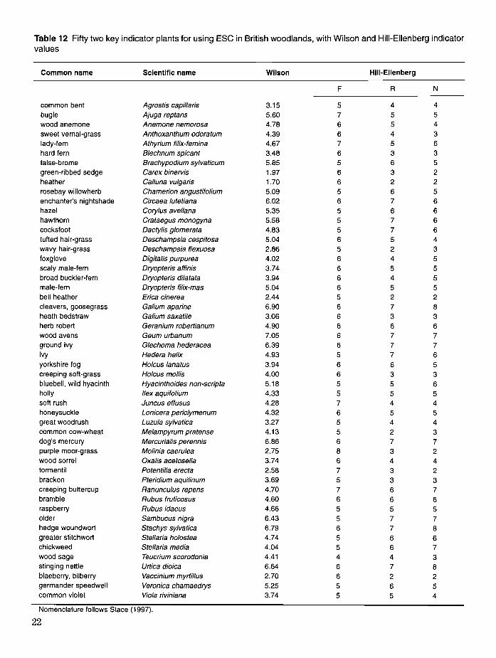
Table 12 Fifty two key indicator plants for using ESC in British woodlands, with Wilson and Hill-Ellenberg indicatorvalues

Common name Scientific name Wilson Hill-Ellenberg

common bent Agrostis capillaris 3.15

F

5

R

4

N

4bugle Ajuga reptans 5.60 7 5 5wood anemone Anemone nemorosa 4.78 6 5 4sweet vernal-grass Anthoxanthum odoratum 4.39 6 4 3lady-fern Athyrium filix-femina 4.67 7 5 6hard fern Blechnum spicant 3.48 6 3 3false-brome Brachypodium sylvaticum 5.85 5 6 5green-ribbed sedge Carex binervis 1.97 6 3 2heather Calluna vulgaris 1.70 6 2 2rosebay willowherb Chamerion angustifolium 5.09 5 6 5enchanter's nightshade Circaea lutetiana 6.02 6 7 6hazel Corylus avellana 5.35 5 6 6hawthorn Crataegus monogyna 5.58 5 7 6cocksfoot Dactylis glomerata 4.83 5 7 6tufted hair-grass Deschampsia cespitosa 5.04 6 5 4wavy hair-grass Deschampsia flexuosa 2.86 5 2 3foxglove Digitalis purpurea 4.02 6 4 5scaly male-fern Dryopteris affinis 3.74 6 5 5broad buckler-fern Dryopteris dilatata 3.94 6 4 5male-fern Dryopteris filix-mas 5.04 6 5 5bell heather Erica cinerea 2.44 5 2 2cleavers, goosegrass Galium aparine 6.90 6 7 8heath bedstraw Galium saxatile 3.06 6 3 3herb robert Geranium robertianum 4.90 6 6 6wood avens Geum urbanum 7.05 6 7 7ground ivy Glechoma hederacea 6.39 6 7 7ivy Hedera helix 4.93 5 7 6yorkshire fog Holcus lanatus 3.94 6 6 5creeping soft-grass Holcus mollis 4.00 6 3 3bluebell, wild hyacinth Hyacinthoides non-scripta 5.18 5 5 6holly Ilex aquifolium 4.33 5 5 5soft rush Juncus eflusus 4.28 7 4 4honeysuckle Lonicera periclymenum 4.32 6 5 5great woodrush Luzula sylvatica 3.27 5 4 4common cow-wheat Melampyrum pratense 4.13 5 2 3dog's mercury Mercurialis perennis 6.86 6 7 7purple moor-grass Molinia caerulea 2.75 8 3 2wood sorrel Oxalis acetosella 3.74 6 4 4tormentil Potentilla erecta 2.58 7 3 2bracken Pteridium aquilinum 3.69 5 3 3creeping buttercup Ranunculus repens 4.70 7 6 7bramble Rubus fruticosus 4.60 6 6 6raspberry Rubus idaeus 4.66 5 5 5elder Sambucus nigra 6.43 5 7 7hedge woundwort Stachys sylvatica 6.79 6 7 8greater stitchwort Stellaria holostea 4.74 5 6 6chickweed Stellaria media 4.04 5 6 7wood sage Teucrium scorodonia 4.41 4 4 3stinging nettle Urtica dioica 6.64 6 7 8blaeberry, bilberry Vaccinium myrtillus 2.70 6 2 2germander speedwell Veronica chamaedrys 5.25 5 6 5common violet Viola riviniana 3.74 5 5 4

Nomenclature follows Stace (1997).

22

Table 13 A further 48 indicator plants for using ESC in British woodlands, with Hill-Ellenberg indicator values

Common name Scientific name Hill-Ellenberg

yarrow Achillea millefoliumF5

R6

N4

ramsons, wild garlic Allium ursinum 6 7 7wild angelica Angelica sylvestris 8 6 5burdock Arctium minus 4 7 5false oat-grass Arrhenatherum elatius 5 7 7marsh marigold Caltha palustris 9 6 4wood sedge Carex sylvatica 5 6 5common mouse-ear Cerastium fontanum 5 5 4golden saxifrage Chrysosplenium oppositifolium 9 5 5creeping thistle Cirsium arvense 6 7 6marsh thistle Cirsium palustre 8 5 4spear thistle Cirsium vulgare 5 6 6pignut Conopodium majus 5 5 5broom Cytisus scoparius 5 4 4crowberry Empetrum nigrum 6 2 1common horsetail Equisetum arvense 6 6 6wood horsetail Equisetum sylvaticum 8 5 5cross-leaved heath Erica tetralix 8 2 1common cotton-grass Eriophorum angustifolium 9 4 1cotton-grass, hare's-tail Ehophorum vaginatum 8 2 1wood spurge Euphorbia amygdaloides 5 6 6sheep's fescue Festuca ovina 5 4 2red fescue Festuca rubra 5 6 5meadow-sweet Filipendula ulmaria 8 6 5common hemp-nettle Galeopsis tetrahit 5 6 6hogweed Heracleum sphondylium 5 7 7slender St John's wort Hypericum pulchrum 5 4 3sharp-flowered rush Juncus acutiflorus 8 4 2compact rush Juncus conglomeratus 7 4 3heath rush Juncus squarrosus 7 2 2yellow archangel Lamiastrum galeobdolon 5 7 6heath woodrush Luzuta multiflora 6 3 3yellow pimpernel Lysimachia nemorum 7 4 5bog myrtle Myrica gale 9 3 2mat-grass Nardus stricta 7 3 2lousewort Pedicularis sylvatica 8 3 2rough meadow-grass Poa trivialis 6 6 6primrose Primula vulgaris 5 6 4lesser celandine Ranunculus ficaria 6 6 6sheep's sorrel Rumex acetosella 5 4 3red campion Silene dioica 6 6 7devil's-bit scabious Succisa pratensis 7 5 2deer-grass, deer-sedge Trichophorum cespitosum 8 2 1white clover Trifolium repens 5 6 6gorse Ulex europaeus 5 5 3cowberry Vaccinium vitis-idaea 5 2 2common valerian Valeriana officinalis 8 6 5wood speedwell Veronica montana 6 6 6

Nomenclature follows Stace (1997).

23

Hill-Ellenberg values and is therefore o f uncertain reliability. Where available, the Wilson nutrient value has been given priority over the Hill- Ellenberg R+N value. Location on the moisture axis is based on the Hill-Ellenberg F value.

In the short-cut method at least the five most abundant plants are identified and listed in order o f abundance (cover percentage). The moisture and nutrient regimes o f the site are judged from an informal ‘weighted average’ o f the cells occupied by the plants on Table 14. For example if the five most abundant plants were broad buckler-fem (50%), creeping soft-grass (30%), wood sorrel (10%), bracken (10%) and tufted hair-grass (5%), the weighted average soil quality indicated would be Moist Medium.

Numerical method for assessing soil moisture regimeThe Hill-Ellenberg F values could be used to calculate a weighted mean value for soil moisture in the same way as the R+N value is used for soil nutrients, but this method is not considered sufficiently precise for most woodlands. The range o f values is between 5 and 6 for most commercial plantations and under-estimates the variation in moisture regime evident in the soil. This is in spite o f the fact that the method works well for non-woodland vegetation and is effective at differentiating the ‘wet woodlands’ from the other NVC woodlands (see chapter 8). It is recommended therefore, that the use o f indicator plants for soil moisture regime should be confined to the use o f Table 14 as a check or refinement for the assessment made by the methods given in chapters 3 and 5.

Numerical method for assessing soil nutrient regimeThis method produces a weighted average indicator value for a site from a description o f the ground vegetation using the method given below. The calculation o f the weighted average indicator

value for a site involves, for each plant in turn, multiplying the abundance by the indicator value, summing the products and finally dividing by the sum o f the abundances. The calculation is performed most easily within the ESC-DSS. The ESC-DSS calculates the weighted average indicator values and identifies the nutrient class using Table 15, having applied the rule to choose between Wilson and Hill-Ellenberg (see footnote to Table).

Method of obtaining quantitative data on indicator plants for ESCA good description o f the vegetation is obtained from 10 quadrats each 2 x 2 m in size, arranged systematically over the site. The number o f quadrats may be reduced to five if the vegetation looks fairly uniform. All vascular plants (flowering plants and ferns) should be identified and their abundance recorded as a percentage. Shrubs over 1 m tall should be treated as a separate layer, otherwise bracken, ferns, grasses and herbs can be recorded in the same ( ‘field’) layer. Bryophytes are usually treated as another ( ‘ground’) layer, but for ESC purposes they can be ignored. Where the field layer is itself layered, e.g. where bracken is present, the sum o f abundance values will often exceed 100 per cent. The percentages should be summed and, if necessary, each species’ value adjusted to produce the appropriate total. The natural tendency is to under-estimate abundance. The ‘abundance charts’ attached to the soil description method (Figure 36) may be helpful. If there is a lot o f bare soil present, and this is not simply the result o f dense bracken, bramble or other tall plants, then the total cover will add up to less than 100 per cent. Where the total cover is less than about 10 per cent the reliability o f the method is open to question, although a larger sample may be a worthwhile expedient.

A suitable form for recording the details o f site and vegetation is given as Figure 35 in Appendix 3.

24

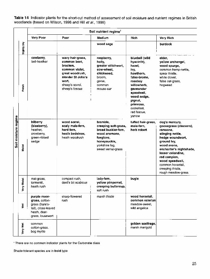
Table 14 Indicator plants for the short-cut method of assessment of soil moisture and nutrient regimes in British woodlands (based on Wilson, 1998 and Hill eta!., 1999)

Soil nutrient regime1

Very Poor Poor Medium Rich Very Rich

Slig

htly

Dry wood sage burdock

cowberry, wavy hair-grass, raspberry, bluebell (wild elder,bell-heather common bent, holly, hyacinth), yellow archangel,

bracken, greater stitchwort, hazel, wood spurge,common violet, cow-wheat, ivy, common hemp-nettle,great woodrush, chickweed, hawthorn, spear thistle,slender St John's broom, false-brome, white clover,wort, gorse, rosebay false oat-grass,

c .in

sheep's sorrel, common willowherb, hogweedo>ii sheep's fescue mouse-ear germander

speedwell,wood sedge,pignut,primrose,cocksfoot,red fescue,yarrow

bilberry wood sorrel, bramble, tufted hair-grass, dog's mercury,(blaeberry), scaly male-fern, creeping soft-grass, male-fern, goosegrass (cleavers),heather, hard fern, broad buckler-fern, herb robert ramsons,crowberry, heath bedstraw, wood anemone, stinging nettle,green-ribbed heath woodrush foxglove, hedge woundwort,sedge honeysuckle, ground Ivy,

til yorkshire fog, wood avens,o£ sweet vernal-grass enchanter's nightshade,

lesser celandine,red campion,wood speedwell,common horsetail,creeping thistle,rough meadow-grass

V) mat-grass, compact rush, lady-fern, bugle0S tormentil, devil's bit scabious yellow pimpernel,t heath rush creeping buttercup,

soft rush

purple moor- sharp-flowered marsh thistle wood horsetail,grass, cotton- rush common valerian

« grass (hare's- meadow-sweet,3 tail), cross-leaved wild angelica

heath, deer-grass, lousewort

© common golden saxifrage,3 cotton-grass, marsh marigoldc©> bog myrtle

' There are no common indicator plants for the Carbonate class

Shade-tolerant species are in bold type

25

Table 15 Conversion of the weighted mean indicator value for a site to the nutrient class

Nutrient class Very Poor Poor Medium Rich Very Rich Carbonate

Wilson nutrient indicator value <2.8 2.8-3.9 3.9—4.8 4.8-6.0 >6 .0 no data

Hill-Ellenberg R+N value <5.7 5.7-7.7 7.7-9.7 9.7-11.7 >11.7 R value >6.0

N value <4.5

Rule for choosing between Wilson and Hill-Ellenberg values: Where plants with Wilson values constitute 60 per cent or more of the vegetation of a site the Wilson values are preferred. For sites where plants with Wilson values have less than 60 per cent of the vegetation cover, the Hill-Ellenberg R+N values are used (for details of the method see Chapter 8).

26

Chapter 7

Choice of tree species for ESC site types

Introduction: species suitabilityChoice o f tree species is one o f the most important silvicultural decisions the manager makes and it is affected by ecological, financial and practical considerations. The advice that fo llows provides a list o f species that are ecologically suited to particular climates and soil qualities in Britain and capable o f producing good quality timber. The timber-producing capability does not, however, extend to the Sub-alpine zone and trees cannot grow at all in the Alpine zone.

Tree species suitability can be represented in three classes, very suitable, suitable and unsuitable. For each species the range o f values o f each climatic factor is divided into three sectors and labelled with these ratings (Figures 9 to 12). The classes o f soil moisture regime and soil nutrient regime are rated in a similar way (Figures 13 and 14). When combining the ratings o f each factor to arrive at an overall suitability for a particular site, it is the lowest rating that determines the outcome. Differences from Pyatt and Suarez (1997) reflect new climatic data and their class boundaries, and refinements o f the earlier advice. The term very suitable is now preferred to optimal.

In very suitable conditions a tree species is expected to grow at a rate given by the upper third o f the range o f yield class shown in the Yield Models (Edwards and Christie, 1981) and to be capable o f doing so without undue risk o f disease or pest attack to an age well above that o f normal financial maturity. It may thus be an appropriate species/site combination to choose for long-term retention for landscape or wildlife reasons. The species will also be capable o f producing viable seed for natural regeneration (see below). In suitable conditions, unless limited by lack o f warmth, a tree species is either expected to grow at a rate given by the middle third o f the range o f

yield class in the Yield Models, or it is expected to grow well early in its life but with reduced growth in the later part o f the rotation. Where rate o f growth is limited by lack o f warmth, the species should still be capable o f growing to biological maturity but natural regeneration w ill be unreliable. Where there are increased risks o f injury from pests, disease or drought, then the species is considered incapable o f growing to normal biological maturity. It should not be considered appropriate for long-term retentions. A species is considered unsuitable when the risks o f it being incapable o f producing sawlogs are too high.

It is assumed that climatic and soil factors cannot compensate for one another. Thus a very suitable climate cannot compensate in terms o f yield for an unsuitable soil quality, and vice versa. Similarly, if any one factor, climatic or soil, is unsuitable, a favourable rating o f any or all o f the other factors cannot make the site suitable for the species. This does not, o f course, preclude the possibility that appropriate management o f a site could be used to upgrade soil quality to achieve a higher rating.

The species suitability criteria are essentially subjective and draw on personal experience in Britain and abroad, in particular British Columbia, together with a wide variety o f literature. Some of the more useful literature, in alphabetical order, is as follows: Aldhous and Low, 1974; Anderson, 1950; Anon., 1991a; Anon., 1991b; Day, 1957; Evans, 1984; Franklin and Dymess, 1973; Krajina, 1969; Lines, 1987; Macdonald, 1952; Macdonald et al., 1957; Savill, 1991; Schmidt, 1957; Weissen et al., 1994; Wood, 1955; Wood and Nimmo, 1962.

In the ESC-DSS the stepped changes in suitability rating have been replaced by smooth ‘response curves’, an example o f which is given as Figure 15.

27

Accumulated temperature (day-degrees >5.0°C)Warm Cool Sub-alpine

Species >1800 1800-1475 1475-1200 1200-975 97 5 -7 7 5 775-575 57 5 -3 7 5

SP

CP

LP

MCP

SS RSS, WSS RSS.W WSS.SS OSS WSS, QSS QSS QSS QSS ASS

NS m m [EL

JL

DF

GF

NF

PSF

WH

RC

RSQ

SOK

POK

BE

AH

SY

WEM

SC

SBI

DBI

ASP

PO

CAR

HBM

SLI

WCH

RAU

KEY Verv suitable [ I S u i t a b l e I Unsuitable

For explanation of species abbreviations and seed origins see Appendix 6. Where seed origins are given, these are the only ones recommended.

Figure 9 Suitability of tree species by accumulated temperature.

28

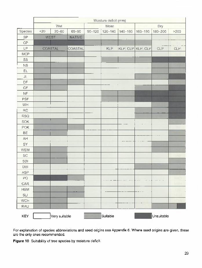
Moisture deficit (mm)

Wet Moist DrySpecies <20 20-60 60-90 90-120 120-140 140-160 160-180 180-200 >200

SP WEST NATIVE

CP

LP COASTAL COASTAL KLP KLP, CLP KLP, CLP CLP CLPMCP

SS

NS

EL

JL

DF

GF

NF

PSF

WH

RC

RSQ

SOK

POK

BE

AH

SY

WEM

SC

SBI

DBI

ASP

PO

CAR

HBM

SLI

WCH

RAU

KEY Very suitable Suitable I Unsuitable

For explanation ot species abbreviations and seed origins see Appendix 6. Where seed origins are given, these are the only ones recommended.

Figure 10 Suitability of tree species by moisture deficit.

29

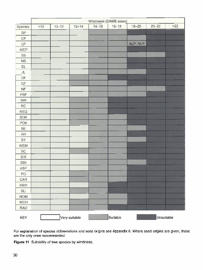
For explanation of species abbreviations and seed origins see Appendix 6. Where seed origins are given, these are the only ones recommended.

Figure 11 Suitability of tree species by windiness.

30

Continentality

Species <5 5-7 7-9 >9

SP

CP

LP ALP, NLP, KLP

MCP

SS

NS

EL

JL

DF

GF

NF

PSF

WH

RC

RSQ

SOK

POK

BE

AH

SY

WEM

SC

SBI

DBI

ASP

PO

CAR

HBM

SLI

NOM

WCH

RAU

KEY Very suitable Suitable

For explanation of species abbreviations and seed origins see Appendix 6. Where seed origins are given, these are the only ones recommended.

Figure 12 Suitability of tree species by continentality.

31

KEY Very suitable Suitable 1 Unsuitable

For explanation of species abbreviations and seed origins see Appendix 6. Where seed origins are given, these are the only ones recommended.

Figure 13 Suitability of tree species by soil moisture regime.

32

Unsuitable

For explanation of species abbreviations and seed origins see Appendix 6. Where seed origins are given, these are the only ones recommended.

Figure 14 Suitability of tree species by soil nutrient regime.

33

The uppermost curve shows how yield class is assumed to be related to accumulated temp­erature, given that other conditions o f climate and soil are ideal for the species (within British conditions). This is termed the ‘potential yield class’. The remaining curves show how the potential yield class o f the species is held to be affected by variation in the other climatic and soil factors. Here the vertical axis ranges from 0 to 1. In relation to the suitability class system, the change from very suitable to suitable usually coincides with a ratio o f 0.75 and the change from suitable to unsuitable with a ratio o f 0.5.

The ESC-DSS predicts yield class in the following way. For a particular site the climatic values are calculated and the classes o f soil moisture and nutrient regime are determined. Each value is marked on the horizontal axes and the value o f potential yield class and the values o f the ratios (from the other curves) are read off. Whichever is the lowest ratio is then multiplied by the potential yield class to obtain the predicted yield class.

The method is based on the assumption that lack o f warmth is generally a limiting factor to tree growth in Britain and that when other limiting factors are present it is only the most limiting factor that needs to be taken into account. The method is a departure from the traditional view that sites are a complex combination o f multiple factors each o f which can affect the operation o f the others. The new method is relatively easy to program, but its validity remains to be proved.

RisksIn the species suitability ratings, very suitable site conditions o f a species are equated not only with high yield class but also with low risk o f pests, diseases and abiotic problems. The following site- related risks should be particularly guarded against. Species susceptible to butt-rot on Rich or Very Rich soils are: NS, EL, WH and RC. SP is susceptible to fungal defoliation in Wet climatic zones or where accumulated temperature is <775 day-degrees. Species sensitive to frost include CP, SS (when young), EL, JL, DF, GF, WH, RC, SOK, POK, BE, AH. CP and RAU are unusual in that they are liable to be killed at any age by extreme winter

cold. (A key to species abbreviations is contained in Appendix 6 ‘Glossary o f Terms’.)

Timber qualityIn very suitable site conditions a species is also expected to produce stems o f good form and timber o f good quality if managed appropriately. For some species certain climatic and soil conditions can be expected to lead to timber quality problems and should be avoided. The following species should not be planted on ‘sunny slopes’ (see Table 7) because o f the risk o f developing drought cracks in the stem: NF, PSF, GF. Coarse branching and poor stem form tends to be a problem in SP, LP, WH, SBI and DBI on Rich or Very Rich soils.

Natural regenerationThe capacity for natural regeneration o f a tree or stand depends upon the production o f viable seed, appropriate conditions on the forest floor for germination (the ‘seedbed’) and adequate light for the subsequent growth o f the seedlings. The first two o f these depend on site conditions that can be specified in ESC. Broadly speaking, very suitable site conditions are likely to lead to the production o f plentiful seed once the tree has reached the necessary age. Where the climate and especially the warmth is only suitable for the species, production o f seed may be less abundant or at longer intervals o f years. The light requirements (or shade tolerance) o f trees and o f seedlings in particular are indicated in Figure 16, based on Hill et al. (1999). The shade tolerance o f a few species, including ash, is somewhat higher in the seedling/sapling stages than at greater age. The most shade tolerant species, including beech and western hemlock, actually benefit from some shading in the early years, as indicated in Figure 16.

Included in ‘seedbed conditions’ is the competition the seedling suffers from other plants (weed growth). This again is predictable from ESC soil quality. Although more research is required on the complexity o f British conditions, natural regeneration is more readily achieved where weed

34

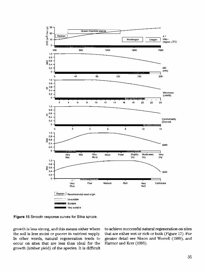
1.00.0 -

. 0.6 - >0.4 -

0.2 -

0 -

1.00.8 -

Z 0.6 w0.4 -

0.2 -

0

Very WeiWei

Very Moist Moisl

Windiness(DAMS)

8 10 12 14 16 18 20 22 24

Conlinentality(Conrad)

SMR

Fresh Slightly Moderately Very Dry Dry Dry

SNR

Very Poor Medium RichPoor

VeryRich

Carbonate

Alaskan~| Recommended seed origin

Unsuitable

Suitable

Very suitable

Figure 15 Smooth response curves for Sitka spruce.

growth is less strong, and this means either where the soil is less moist or poorer in nutrient supply. In other words, natural regeneration tends to occur on sites that are less than ideal for the growth (timber yield) o f the species. It is difficult

to achieve successful natural regeneration on sites that are either wet or rich or both (Figure 17). For greater detail see Nixon and Worrell (1999), and Harmer and Kerr (1995).

35

Light (full shade = 1, full light = 9)

For explanation of species abbreviations and seed origins see Appendix 6.* For these species partial overhead cover is beneficial in the early years.

Figure 16 Relative shade tolerance of tree species in Britain (based on Hill ef al., 1999),

36

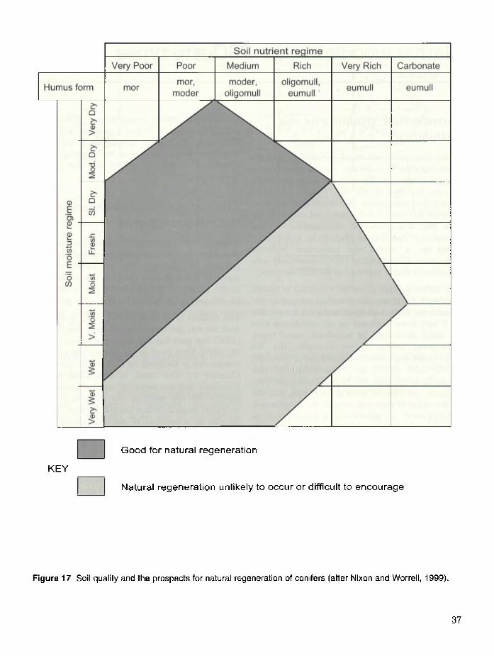
K E Y

G o od fo r n a tu ra l re g e n e ra tio n

N a tu ra l re g e n e ra tio n u n like ly to o c c u r o r d iffic u lt to e n c o u ra g e

Figure 17 Soil quality and the prospects for natural regeneration of conifers (after Nixon and Worrell, 1999).

37

Chapter 8

Native woodlands for ESC site types

Introduction: climate and soil suitabilityWhen new native woodland is being created the main objective is to develop natural character by using a community o f locally native tree and shrub species matched to the site. Natural character means that the ground vegetation that develops beneath the trees is in harmony not only with the site but also with the composition o f the overstorey. This is most likely to be achieved by using as a model the particular National Vegetation Classification (NVC) woodland sub­community that is matched to the ESC site type.

The different types o f native woodland in Britain (Rodwell, 1991) are distributed in relation to site conditions, both at national and local scales. The NVC lays more emphasis on site conditions than on strict definitions o f woodland ‘stand types’ (Peterken, 1981), As an example, the W9 ash-rowan-dog’s mercury woodland is described by Rodwell (1991) as characteristic o f per­manently moist, base-rich brown earth soils in the uplands, yet due to natural processes and the intervention o f man, can actually be an ashwood, a birchwood, an alderwood, a beechwood, an oakwood, an elmwood or even a sycamore wood. Rodwell (1991) described the distribution o f woodlands in terms o f three main climatic zones and three soil groups. The climatic trend is from the cooler wetter north-west to the warmer drier south-east. The soil trend is from calcareous soils through brown earths o f low base-status to very acid rankers and podzolic soils.

The climatic and soil relationships with NVC woodlands are made more explicit by Whitbread and Kirby (1992) and by Rodwell and Patterson (1994). The latter include simple maps o f ‘upland’ and ‘lowland’ climatic zones. It is still surprisingly difficult to visualise the differences in site quality between communities and between sub­

communities within communities. However, it should be possible to find a position within the ESC ‘cube o f ecospace’ appropriate to each NVC woodland. In practice, it is the location o f the woodlands on the soil quality grid that is most interesting.

Linking native woodlands with the soil quality gridRodwell (1991) provided floristic lists for each woodland sub-community compiled from a number o f quadrats. The proportion o f the quadrats in which each plant occurred was given as the frequency in five classes (I = 1-20%, II = 21—40% and so on to V = 81-100%).

The method used here to link NVC woodlands with the soil quality grid is similar to that o f Pyatt (1997) but uses the Hill-Ellenberg values (Hill et al., 1999). Each plant in the floristic list o f a sub­community is assigned its F, R and N value (see Chapter 6). The value is multiplied by the frequency and the resulting sum o f products is divided by the sum o f the frequencies. The weighted mean indicator value for F (mF) is used directly as a measure o f the characteristic soil moisture regime for the sub-community. The weighted mean values for R and N are added together (mR+mN) and used as the measure o f soil nutrient regime. Wilson (1998) showed that mR and mN, based on the abundance o f each plant in his plots, were closely related to soil nutrient regime as determined by soil chemical analysis. Figure 18 shows the location o f each NVC woodland sub-community on the soil quality grid and the main groups o f woodlands (broad stand types) are delineated by boxes. The distribution of the sub-communities on the grid is discussed in detail by Pyatt (1997).

38

R + N

Figure 18 Ordination of NVC woodland sub-communities W1-W20 on scales of F (‘soil moisture’) and R+N (‘soil nutrients’) with approximate boundaries (broken vertical lines) of soil nutrient classes. Species indicator values from Hill et al., 1999.

Separating the communities by climatic zonesPlacing all the woodland sub-communities together on Figure 18 appears complicated because it does not make use o f the climatic factors to separate upland and lowland communities. In practice the climatic relat­ionships are not very precise and communities labelled ‘upland’ or ‘lowland’ by Rodwell and Patterson (1994) can occur in close geographical proximity (Hall, 1998). Nevertheless the distinction is maintained in the interests o f clarity in Figures 19-22. Here only the communities are shown, the size and location o f each box being based subjectively on the spread o f the component sub-communities. In addition to the main lowland/upland split, two communities o f scrub woodland (W19 juniper and W20 willow) are assigned to the Sub-alpine zone. For additional clarity the beechwoods and the lowland ashwoods

and oakwoods are shown on separate Figures, although their climatic zones undoubtedly overlap. The names o f the woodlands given are those o f Rodwell and Patterson (1994).

Suitability ranges of all six ESC site factorsThe suitable range o f each climatic and soil factor for all NVC woodlands W1-W20 is shown in Figures 23-28. The soil requirements o f the woodlands are more critical than the climatic requirements. Where possible, the requirements o f individual sub-communities are shown separately. Only two classes o f suitability are given. In suitable conditions the woodland can be expected to regenerate itself. In unsuitable conditions natural regeneration o f either the tree species or some o f the characteristic species o f the ground vegetation would not occur.

39

In the ESC-DSS, the method o f choosing NVC suitability classes in a similar way to those used woodland communities appropriate to site types for individual tree species (see Chapter 7). uses ‘smooth response curves’ derived from these

Soil nutrient regimeVery Poor Poor Medium Rich Very Rich Carbonate

<DEcno

oEoW

£QT3O

£o

.cw0

I/I

o5

£0>

W16Oak-birch with bilberry/ blaeberry

W10Mixedbroadleaved with bluebell/ wild hyacinth

W8Mixedbroadleaved with dog’s mercury

W6Alder withstingingnettle

W1Sallow withmarshbedstraw

Figure 19 Very suitable soil quality for native oak, ash and alder woodlands in Warm dry and Warm moist climatic zones (the 'Lowland Zone' of FC Bulletin 112 (Rodwell and Patterson, 1994)).

40

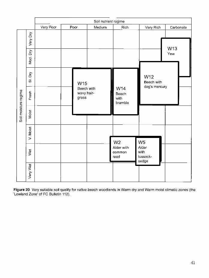
Soil nutrient regime

Very Poor Poor Medium Rich Very Rich Carbonate

CDECDCDL_0IDtoOEo

CO

Q

0>

£QTDO

QCO

.cw0

W13Yew

W15Beech with wavy hair- grass

W14Beechwithbramble

W12Beech with dog's mercury

o

>W2

Alder withcommonreed

W5Alderwithtussock-sedge

Figure 20 Very suitable soil quality for native beech woodlands in Warm dry and Warm moist climatic zones (the 'Lowland Zone' of FC Bulletin 112).

41

Soil nutrient regimeVery Poor Poor Medium Rich Very Rich Carbonate

£■Q

0>

Q■do

0Ea)00D00OEoco

Q

0>

W18Scots pine with heather

W17Oak-birchwithbilberry/blaeberry

W11O ak- birch with bluebell/ wildhyacinth

W9Mixedbroad­leaveddog’smercury

with

W4Birch with purple moor- grass

W7Alder-ash with yellow pimpernel

Figure 21 Very suitable soil quality for native woodlands in Warm wet, Cool moist and Cool wet climatic zones (the 'Upland Zone' of FC Bulletin 112).

42

Soil nutrient regimeVery Poor Poor Medium Rich Very Rich Carbonate

Soil

moi

stur

e re

gim

e

Very

D

ryM

od.

Dry

SI.

Dry

Fres

h W19Juniper with wood sorrel

Moi

st W20Salixlapponum-

V. M

oist

Luzulasylvatica

QJ§

Very

W

et

Figure 22 Very suitable soil quality for native scrub woodlands in the Sub-alpine zone (the ‘Upland juniper zone’ of FC Bulletin 112).

43

KEY Suitable Unsuitable

Figure 23 Suitability of native woodlands W1-W20 by accumulated temperature.

44

KEY Suitable llln s u ita b le

Figure 24 Suitability of native woodlands W1-W20 by moisture deficit.

45

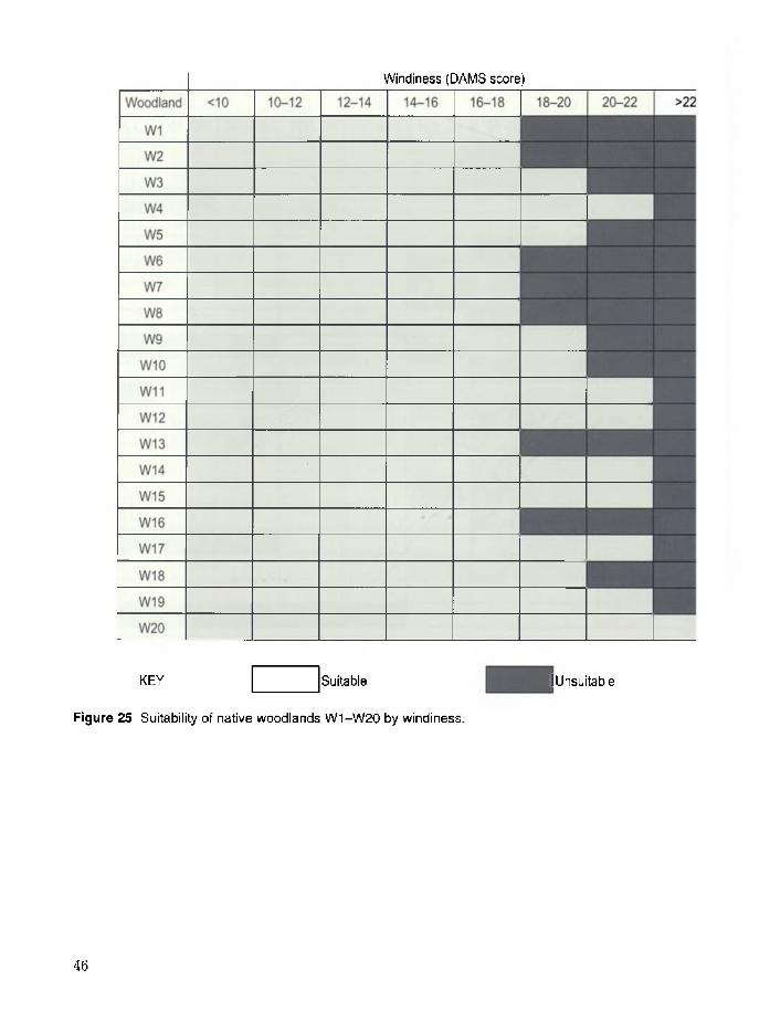
Windiness (DAMS score)

KEY Suitable lU nsu ita b le

Figure 25 Suitability of native woodlands W1-W20 by windiness.

4b

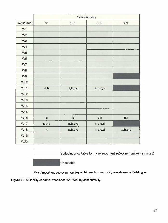
Continentality

Woodland <5 5 -7 7 -9 >9

W1

W2

W3

W4

W5

W6

W7

W8

W9

W10

W11 a.b a,b,c,d a.b.c.d

W12

W13

W14

W15

W16 b b b,a a,b

W17 a,b,c a,b,c,d a,b,c,d

W18 e a,b,c,d a,b,c,d a,b,c,d

W19

W20

Suitable, or suitable for more important sub-communities (as listed)

Most important sub-communities within each community are shown in bold type

Figure 26 Suitability of native woodlands W1-W20 by continentality.

47

Soil moisture regime

Woodland Very Wet Wet Very Moist Moist Fresh SlightlyDry

ModeratelyDry

Very Dry

W1

W2 a,b a,b

W3

W4 c,b c,b b,a a

W5 a,b,c a,b,c c

W6 a.b a,b,d,e d.e

W7 b a,b c

W8 a-d,e-g a-d,e-g a-d,e-g

W9 a,b a,b a,b

W10 a,b,c,d,e a,b,c,d,e a,b,c,d,e a,b,c,d,e

W11 a,b,c,d a.b.c.d a .bc.d

W12 a,b a,b,c a,b,c

W13 a,b a,b a.b

W14

W15 a.b.c.d a.b.c.d a.b.c.d

W16 a,b a,b a,b

W17 a,d b.c b,c

W18 d d,e b,c,e a

W19 a,b a,b

W20

KEY

Suitable, or suitable for more important sub-communities (as listed)

Suitable for lesser sub-communities (as listed)

Unsuitable

Most important sub-communities within each community are shown in bold type

Figure 27 Suitability of native woodlands W1-W20 by soil moisture regime.

48

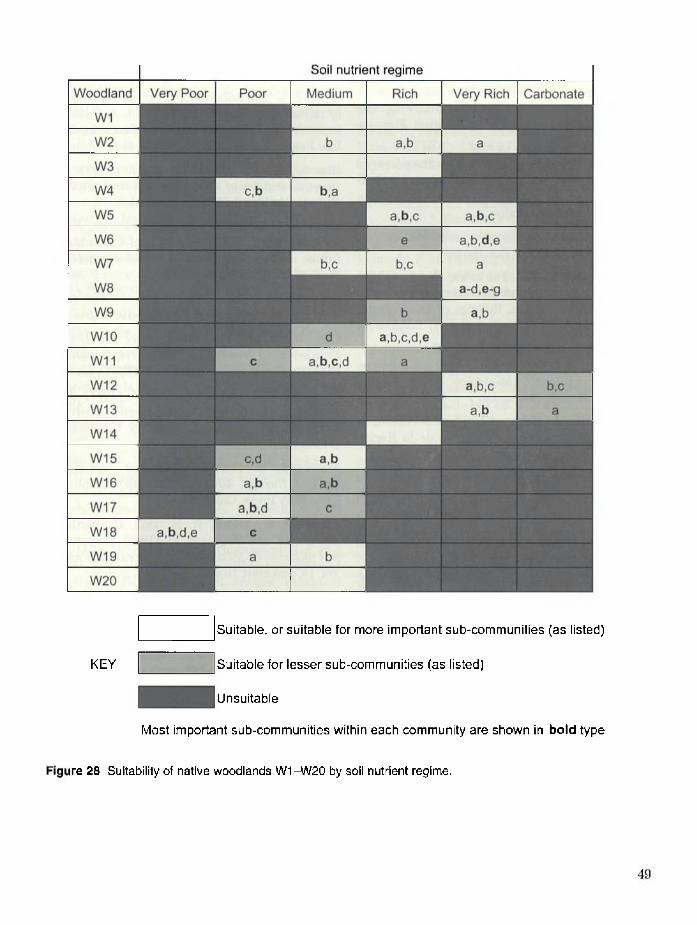
KEY

Suitable, or suitable for more important sub-communities (as listed)

Suitable for lesser sub-communities (as listed)

Unsuitable

Most important sub-communities within each community are shown in bold type

re 28 Suitability of native woodlands W1-W20 by soil nutrient regime.

R e fe re n c e sAdamson, J. K , Homung, M., Pyatt, D. G. and Anderson, A. R. (1987). Changes in solute chemistry o f drainage waters following the clearfelling o f a Sitka spruce plantation. Forestry 60 (2), 165-177.

Aldhous, J. R. and Low, A. J. (1974). The potential o f western hemlock, western red cedar, grand f i r and noble f i r in Brita in . Forestry Commission Bulletin 49. HMSO, London.

Anderson, M. L. (1950). The selection o f tree species. Oliver & Boyd, Edinburgh.

Anderson, M. L. and Fairbaim, W. A. (1955). D iv is ion o f Scotland into c lim atic sub-regions as an aid to silviculture. Bulletin o f the Forestry Department No. 1. University o f Edinburgh, Scotland.

Anon. (1991a). Le f ich ie r ecologique des essences, 1: texte explicatif. Ministere de la Region Wallonne, Namur, Belgium.

Anon. (1991b). Le f ich ie r ecologique des essences, 2: le f ich ie r ecologique. Ministere de la Region Wallonne, Namur, Belgium.

Barrow, E., Hulme, M. and Jiang, T. (1993). A 1961-90 baseline climatology and fu tu re climate change scenarios f o r Great B rita in and Europe. Part I : 1961-90 Great B r ita in baselineclimatology. Climate Research Unit, University o f East Anglia, Norwich. 50 pp.

Bendelow, V. C. and Hartnup, R. (1980). Clim atic classification o f England and Wales. Soil Survey Technical Monograph No. 15. Rothamsted Experimental Station, Harpenden. 27 pp.

Binns, W. O., Mayhead, G. J. and MacKenzie, J. M. (1980). N u trien t deficiencies o f conifers in B ritish forests. Forestry Commission Leaflet 76. HMSO, London.

Birse, E. L. (1971). Assessment o f c lim a tic conditions in Scotland, 3: The b ioclim atic sub- regions. Macaulay Land Use Research Institute, Aberdeen. 12 pp.

Birse, E. L. and Dry, F. T. (1970). Assessment o f clim atic conditions in Scotland, 1: Based on accumidated temperature and potential ivater

deficit. Macaulay Land Use Research Institute, Aberdeen. 25 pp.

Birse, E. L. and Robertson, L. (1970). Assessment o f c lim atic conditions in Scotland, 2: Based on exposure and accumulated frost. Macaulay Land Use Research Institute, Aberdeen. 41 pp.

Blarney, M. and Grey-Wilson, C. (1989). The illustrated f lo ra o f Great B rita in and northern Europe. Hodder & Stoughton, London.

Brethes, A., Brun, J-J., Jabiol, B., Ponge, J. and Toutain, F. (1995). Classification o f forest humus forms: a French proposal. Annales des Sciences Forestieres 52 (6), 535-546.

Cajander, A. K. (1926). The theory o f forest types. Acta Forestalia Fennica 29 (3), 1-108.

Day, W. R. (1957). Sitka spruce in B ritish Colum bia: a study in forest relationships., Forestry Commission Bulletin 28. HMSO, London.

Edwards, P. N. and Christie, J. M. (1981). Yield models f o r forest management. Forestry Commission Booklet 48. Forestry Commission, Edinburgh.

Ellenberg, H. (1988). Vegetation ecology o f Central Europe, 4th edtn (English). Cambridge University Press, Cambridge.

Ellenberg, H., Weber, H. E., Dull, R., Wirth, V., Wemer, W. and Paulissen, D. (1992). Zeigerwerte vonpflanzen in Mitteleuropa. Scripta Geobotanica Vol. 18, 2nd edtn. Goltze, Gottingen. 258 pp.

Evans, J. (1984). S ilv icu ltu re o f broadleaved ivoodland. Forestry Commission Bulletin 62. HMSO, London.

Fairbaim, W. A. (1960). Climatic zonation in England and Wales. In ternational Journal o f Bioclim ato logy and B iom eteorology IV (II), section C. 20 pp.

Field Studies Council (1988). Key to common grasses. Field Studies Council, Preston Montford, Montford Bridge, Shrewsbury, SY4 1HW.

Field Studies Council (1998a). A key to plants common in woodland. Field Studies Council, Preston Montford, Montford Bridge, Shrewsbury, SY4 1HW.

50

Field Studies Council (1998b). A key to plants common on moorlands. Field Studies Council, Preston Montford, Montford Bridge, Shrewsbury, SY4 1HW.

Forestry Commission (1998). The UK forestry standard. Forestry Commission, Edinburgh.

Forestry Commission (2001). Ecolog ica l site classifica tion : a PC-based decision support system fo r B ritish forests. Forestry Commission, Edinburgh. (Manual + CD-ROM.)

Franklin, J. F. and Dymess, C. T. (1973). Natural vegetation o f Oregon and Washington. USDA Forest Service General Technical Report PNW-8. USDA Forest Service, Portland, Oregon.

Garrard, I. and Streeter, D. (1998). The wild flowers o f the B ritish Isles. Midsummer Books, London.

Gilchrist, W. (1872). On the soils best suited for the different kinds o f forest trees, as indicated by the plants that grow naturally upon them. Transactions o f the Royal A rboricu ltura l Society VI, 296-303.

Green, R. N., Trowbridge, R. L. and Klinka, K. (1993). Towards a taxonomic classification o f humus form s. Forest Science Monograph 29. Society o f American Foresters, Bethesda, MD. 49pp.

Hall, D. G. M., Reeve, M. G., Thomasson, A. J. and Wright, V. F. (1977). Water retention, porosity and density o f f ie ld soils. Soil Survey Technical Monograph No. 9. Rothamsted Experimental Station, Harpenden.

Hall, J. (1998). A n analysis o f N a tiona l Vegetation Classification survey data. Report No. 272. Joint Nature Conservation Committee, Northminster House, Peterborough.

Harmer, R. and Kerr, G. (1995). N atura l regeneration o f broadleaved trees. Forestry Commission Research Information Note 275. Forestry Commission, Edinburgh.

Hill, M. O., Mountford, J. 0., Roy, D. B. and Bunce, R. G. H. (1999). Ellenberg’s ind ica tor values fo r B ritish plants. ECOFACT Volume 2, Technical Annex. Institute o f Terrestrial Ecology,Huntingdon.

Hodgson, J. M. (1974). S oil Su'rvey f ie ld handbook. Technical Monograph No. 5. Soil Survey o f England and Wales, Harpenden. (3rd edtn., 1997).

Jabiol, B., Brethes, A., Ponge, J-F., Toutain, F. and Brun, J-J. (1995). L ’humus sous toutes sesfoimes. Ecole Nationale du Genie Rural, des Eaux et des Forets, Nancy. 63 pp.

Katzensteiner, K., Englisch, M. and Hager, H. (in preparation.). Taxonomy o f forest humus forms, a proposal for a European classification.

Kennedy, F. M. (2001). The identification o f soils f o r forestry. Forestry Commission Field Book 19. Forestry Commission, Edinburgh.

Klinka, K , Krajina, V. J., Ceska, A. and Scagel, A. M. (1989). Ind icator plants o f coastal B ritish Columbia. UBC Press, Vancouver, BC. 288 pp.

Krajina, V. J. (1969). Ecology o f forest trees in British Columbia. In, Ecology o f western North America, Vol. 2,1-146, ed. V. J. Krajina. University o f British Columbia, Department o f Botany.

Landon, J. R. (1988). Toward a standard field assessment o f soil texture for mineral soils. Soil Survey and Land Evaluation 8, 161-165.

Lines, R. (1987). Choice o f seed orig ins fo r the m ain fo res t species in B rita in . Forestry Commission Bulletin 66. HMSO, London.

Macdonald, J. (1952). The place o f north-western American conifers in British Forestry. S ixth B ritish Commonwealth Forestry Conference, Canada, Item 7a Silviculture. 21 pp.

Macdonald, J., Wood, R. F., Edwards, M. V. and Aldhous, J. R. (1957). E xotic forest trees in Great Brita in . Forestry Commission Bulletin 30. HMSO, London.

Nixon, C. J. and Worrell, R. (1999). The potential f o r the natural regeneration o f conifers in B rita in . Forestry Commission Bulletin 120. Forestry Commission, Edinburgh.

Ontario Institute o f Pedology (1985). Field manual f o r describing soils. 3"' edition. Ontario Institute o f Pedology and University o f Guelph, Ontario. OIP Publication 85-3.

51

Peterken, G. F. (1981). Woodland conservation and management. Chapman and Hall, London. (21"1 edition, 1993).

Phillips, R. (1980). Grasses, ferns, mosses and lichens o f Great B rita in and Ireland. Pan Books, London.

Pojar, J., Klinka, K. and Meidinger, D. (1987). Biogeoclimatic ecosystem classification in British Columbia. Forest Ecology and Management 22, 119-154.

Pyatt, D. G. (1970). Soil groups o f upland forests. Forestry Commission Forest Record 71. HMSO, London.

Pyatt, D. G. (1977). Guide to site types in forests o f north and m id Wales. Forestry Commission Forest Record 69. HMSO, London.

Pyatt, D. G. (1982). Soil classification. Forestry Commission Research Information Note 68/82/SSN. Forestry Commission, Edinburgh.

Pyatt, D. G. (1997). A site classification for Scottish native woodlands. Botanical Journal o f Scotland 49 (2), 455-467.

Pyatt, D. G. and Smith, K. A. (1983). Water and oxygen regimes o f four soil types at Newcastleton Forest, south Scotland. Journal o f Soil Science 34, 465-482.

Pyatt, D. G., Spencer, J. W., Hutchby, L., Davani, S., Fletcher, J. and Purdy, K. (2001). Applying the ecological site classification in the lowlands - a case study o f the New Forest inclosures. Forestry Commission Technical Paper 33. Forestry Commission, Edinburgh.

Pyatt, D. G. and Suarez, J. C. (1997). A n ecological site classification fo r forestry in Great B rita in ivith special reference to Grampian, Scotland. Forestry Commission Technical Paper 20. Forestry Commission, Edinburgh.

Quine, C. P. (2000). Estimation o f mean wind climate and probability o f strong winds from assessments o f relative windiness. Forestry 73 (3), 247-258.

Quine, C. P. and White, I. M. S. (1993). Revised ivindiness scores fo r the windthrow hazard classification : the revised scoring method.

Forestry Commission Research Information Note 230. Forestry Commission, Edinburgh.

Quine, C. P. and White, I. M. S. (1994). Using the relationship between rate o f tatter and topographic variables to predict site windiness in upland britain. Forestry 67 (3), 245-256.

Rameau, J. C., Mansion, D. and Dume, G. (1989). Flore forestiere frangaise: guide ecologique illustre; Vol 1: Plaines et collines. Institut pour le Developpement Forestier, Ministere del’Agriculture et de la Peche, Paris. 1785 pp.

Rameau, J. C., Mansion, D. and Dume, G. (1993). Flore fo res tiere frangaise: guide ecologique illustre; Vol 2: Montagues. Institut pour le Developpement Forestier, Ministere del’Agriculture et de la Peche, Paris. 2421 pp.

Ray, D. and Nicoll, B. (1994). Effects o f soil water on root development and stability o f Sitka spruce. Journal o f Experim enta l Botany 46(supplement), 47.

Robson, J. D. and Thomasson, A. J. (1977). Soil ivater regimes. Soil Survey Technical Monograph No. 11. Rothamsted Experimental Station, Harpenden. 57 pp.

Rodwell, J. S. (ed .) (1991). B ritis h p lant com m unities, I : Woodlands and scrub.Cambridge University Press, Cambridge.

Rodwell, J. S. and Patterson, G. S. (1994). Creating new native woodlands. Forestry Commission Bulletin 112. HMSO, London.

Rose, F. (1989). Colour identification guide to the grasses, sedges, rushes and ferns o f the B ritish Isles and north-ivestem Europe. Viking - Penguin Books, London.

Savill, P. S. (1991). The silviculture o f trees used in B rit is h forestry. C.A.B. International, Wallingford.

Schmidt, R. L. (1957). The silvics and plant geography o f the genus Abies. Technical Publication T 46. Department o f Lands and Forests, British Columbia Forest Service.

Stace, C. (1997). New flo ra o f the B r i tish Isles (2"'1 edition). Cambridge University Press, Cambridge.

52

Taylor, C. M. A. (1991). Forest fe rtilisa tion in Brita in . Forestry Commission Bulletin 95. HMSO, London.

Taylor, C. M. A. and Tabbush, P. M. (1990). Nitrogen deficiency in Sitka spruce plantations. Forestry Commission Bulletin 89. HMSO, London.

Thompson, N., Barrie, I. A. and Ayles, M. (1981). The M eteorological O ffice ra in fa ll and evaporation calculation system: MORECS (July 1981). Meteorological O ffice Hydrological Memorandum N45.

Weissen, F., Bronchart, L. and Piret, A. (1994). Guide de boisement des stations forestieres de Wallonie. Direction Generale des Ressources Naturelles et de l ’Environnement, Jambes, Belgium.

Whitbread, A. M. and Kirby, K. J. (1992). Sum maty o f National Vegetation Classification woodland descriptions. UK Nature Conservation No. 4. Joint Nature Conservation Committee, Peterborough.

White, G. S. A., Pyatt, D. G., Quine, C. P., Fletcher, J., Clare, J., Connolly, T. and Worrell, R. (2000). Neiv clim ate data f o r ecological site classification in B ritish forestry. Unpublished paper. Forest Research, Roslin Midlothian.

Wilson, S.M. (1998). The quantification o f soil n u trien t regim e in B ritis h forests and its assessment fro m ground vegetation and humus type. Unpublished PhD thesis, University o f Edinburgh.

Wilson, S. M., Pyatt, D. G., Malcolm, D. C. and Connolly, T. (1998). Ecological site classification: soil nutrient regime in British woodlands. Scottish Forestry 52 (2), 86-92.

Wood, R. F. (1955). Studies o f north-west Am erican forests in relation to s ilv iculture in Great Brita in . Forestry Commission Bulletin 25. HMSO, London.

Wood, R. F. and Nimmo, M. (1962). Chalk doivnland afforestation. Forestry Commission Bulletin 34. HMSO, London.

53

Appendix 1

The assessment of soil texture and available water capacity

As mentioned in Chapter 3, the assessment o f soil texture is a part o f the estimate o f the available water capacity o f soil. The ESC method only requires recognition o f organic, sandy, coarse loamy, fine loamy and clayey textures. Two methods for the assessment o f soil texture are given as Figures 29 and 30. The methods are more detailed than is actually necessary. Both methods should give the same results most o f the time, but individual users tend to prefer one method over the other. After one method has been used on a soil sample, it is a good idea to check the result using the other method. Figure 31 shows how the more detailed classes o f texture given in Figures

29 and 30 are related to the broader ESC classes o f texture.

The available water capacity o f the soil is estimated using the method in Figure 32. Although the method is as simple as possible, it allows for the possible existence o f two different layers within the soil. The method does not cater for soils with a water-table within the rooting zone. Such soils are considered to fall into the Moist to Very Wet classes o f moisture regime and do not need an estimate o f available water capacity.

54

TEXTURE

Start with a 2.5 cm diameter mass of soil at the sticky point. Sticky point is defined as themoisture content at which dry soil being gradually moistened just begins to adhere to the fingers.

Cohesive ball formed?

i Yes

Ball falls apart_ easily?

^ No

Ball rolls intoshort cylinder?

.YesI 'Balls rolls in to . thread?

Yes

Thread bends into U shape?

i 'era

l

Yes

Is U cracked?-

No

Thread rolls into a ring?

^ Yes

Is the ring _____cracked?

NoISignificant sandy feel?

1 No

Significant _____silky/soapy feel?

-► No

“ ► Yes

-► No

-► No Sandy feel predominates?

1 No

Silky/soapy feel predominates?

I

-► Yes

Yes

No

-► No

-► Yes ■Significant silky/soapy feel?

No

-► No1

Y

t

No

Significant sandy feel?

-► Yes . Significant silky/soapy feel?

-► No

-► Yes

-► Yes

-► SAND

-► LOAMY SAND

-► SANDY LOAM

-► SILT LOAM

^ SANDY SILT

Yes

LOAM

SANDY CLAY LOAM

. SILTY CLAY LOAM

-► CLAY LOAM

-► SANDY CLAY

-► SILTY CLAY

-► No -► CLAY

Cylinder = dimension about 5 cm long and 1.5 cm in diameter.Thread = about 13 cm long and 0.6 cm in diameter.Ring = a circle about 2.5 cm in diameter formed from an 8 cm section of thread.

Figure 29 Assessment of soil texture, method 1 (after Landon, 1988).

55

Start with a 2.5 cm diameter mass of soil at the sticky point. Sticky point is defined as themoisture content at which dry soil being gradually moistened just begins to adhere to the fingers.

Sandy-ness Smoothness Stickiness and plasticity

Ball and thread formation Texture

Extremelysandy

Not smooth Not sticky or plastic

Non cohesive balls which collapse easily.

Sand

Not sticky or plastic

Slightly cohesive balls, does not form threads.

Loamy sand

Very sandy Not smooth Not sticky or plastic

Slightly cohesive balls, does not form threads.

Sandy loam

Moderatelysandy

Slightly smooth Slightly sticky and plastic

Moderately cohesive balls, forms threads with great difficulty.

Sandy silt loam

Not smooth Moderately sticky and plastic

Moderately cohesive balls, forms long threads which bend into rings with difficulty. Moderate degree of polish.

Sandy clay loam

Not smooth Very sticky and plastic

Very cohesive balls, forms long threads which bend into rings with difficulty. High degree of polish.

Sandy clay

Slightly tomoderatelysandy

Slightly smooth Moderately sticky and plastic

Very cohesive balls, forms threads which will bend into rings.

Clay loam

Non-sandy to slightly sandy

Very smooth and silky

Slightly sticky and plastic

Moderately cohesive balls, forms threads with great difficulty that have broken appearance. No polish.

Silt loam

Moderately smooth and silky

Moderately sticky and plastic

Moderately cohesive balls, forms threads which will not bend into rings. Moderate degree of polish.

Silty clay loam

Very sticky and plastic

Very cohesive balls and long threads which bend into rings. High degree of oolish.

Silty clay

Not smooth Extremely sticky and plastic

Extremely cohesive balls and long threads which bend into rings easily. High degree of polish.

Clay

Cylinder = dimension about 5 cm long and 1.5 cm in diameter.Thread = about 13 cm long and 0.6 cm in diameter.Ring = a circle about 2.5 cm in diameter formed from an 8 cm section of thread.

Figure 30 Assessment of soil texture, method 2.

56

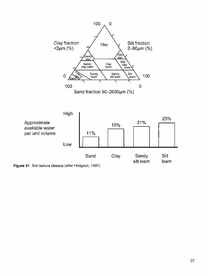
100 „ 0

Clay fraction <2|jm (% )

Silt fraction 2-60|jm (%)

100\ \ \ v

100 0 Sand fraction 60-2000|jm (%)

Approximate available water per unit volume

High

Low

19% 21%

11%

Sand Clay

Figure 31 Soil texture classes (after Hodgson, 1997).

Sandy silt loam

25%

Siltloam

57

Layered soils: For a soil with two very different layers, e.g. a layer of peat over mineral, separate calculations should be made for each layer and summed. (In many cases the two layers will conveniently form the main and secondary rooting zones.)

Step 1: Soil texture of main rooting zone AWC/m

Step 2: Depth of main rooting zone

Multiply the AWC/m by the depth of the main rooting zone in metres, e.g. if the depth is 70 cm multiply by 0.7.(The main rooting zone is that part of the soil that is likely to be uplifted with the root system if the tree is windthrown.)

Step 3: Stoniness of main rooting zone

Soils that are extremely stony (AWC 50 mm/m depth) need no further adjustment.For other soils reduce the AWC obtained so far by the volumetric proportion of stones. For example, if there are 15% stones, multiply value by 0.85.(It is easy to over-estimate the volumetric proportion of stones. Even the extremely stony fluvioglacial gravels with most stones in contact with each other have a maximum of 60% stones by volume, provided the matrix fills the interstices.)

Step 4: Secondary rooting zone

Repeat steps 1-3, for the secondary rooting zone, but finally multiply its contribution to AWC by 0.5.(The secondary rooting zone may have very few roots (e.g. < 1/dm2) but can be a major source of moisture during droughts. If in doubt about depth, err on the generous side.)

Step 5: Add the contributions from the main and secondary rooting zones.

Figure 32 Estimating the available water capacity (AWC) of the soil.

58

Appendix 2

Classification of humus forms

The classification o f humus forms for assessing soil nutrient regime is dealt with in Chapter 5. The classification used (Figure 33) is a simplified version o f that proposed by Katzensteiner et al. (in

preparation). The various forms o f peat are excluded because their soil quality is adequately dealt with by the classification o f forest soil types (Appendix 4) or by the use o f indicator plants.

59

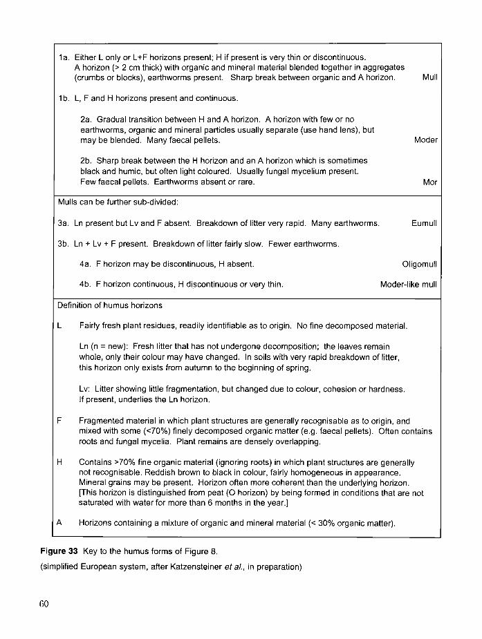
1a. Either L only or L+F horizons present; H if present is very thin or discontinuous.A horizon (> 2 cm thick) with organic and mineral material blended together in aggregates (crumbs or blocks), earthworms present. Sharp break between organic and A horizon. Mull

1b. L, F and H horizons present and continuous.

2a. Gradual transition between H and A horizon. A horizon with few or noearthworms, organic and mineral particles usually separate (use hand lens), butmay be blended. Many faecal pellets. Moder

2b. Sharp break between the FI horizon and an A horizon which is sometimes black and humic, but often light coloured. Usually fungal mycelium present.Few faecal pellets. Earthworms absent or rare. Mor

Mulls can be further sub-divided:

3a. Ln present but Lv and F absent. Breakdown of litter very rapid. Many earthworms. Eumull

3b. Ln + Lv + F present. Breakdown of litter fairly slow. Fewer earthworms.

4a. F horizon may be discontinuous, H absent. Oligomull

4b. F horizon continuous, H discontinuous or very thin. Moder-like mull

Definition of humus horizons

L Fairly fresh plant residues, readily identifiable as to origin. No fine decomposed material.

Ln (n = new): Fresh litter that has not undergone decomposition; the leaves remain whole, only their colour may have changed. In soils with very rapid breakdown of litter, this horizon only exists from autumn to the beginning of spring.

Lv: Litter showing little fragmentation, but changed due to colour, cohesion or hardness.If present, underlies the Ln horizon.

F Fragmented material in which plant structures are generally recognisable as to origin, andmixed with some (<70%) finely decomposed organic matter (e.g. faecal pellets). Often contains roots and fungal mycelia. Plant remains are densely overlapping.

H Contains >70% fine organic material (ignoring roots) in which plant structures are generallynot recognisable. Reddish brown to black in colour, fairly homogeneous in appearance.Mineral grains may be present. Horizon often more coherent than the underlying horizon.[This horizon is distinguished from peat (O horizon) by being formed in conditions that are not saturated with water for more than 6 months in the year.]

A Horizons containing a mixture of organic and mineral material (< 30% organic matter).

Figure 33 Key to the humus forms of Figure 8.

(simplified European system, after Katzensteiner et al., in preparation)

60

Appendix 3

Description of soil profile

Introduction: recording information relevant to soil moisture and nutrient regimesIn order to assess soil moisture and nutrient regimes, the user o f ESC may need to make a simple soil description including soil type, lithology, humus form, rooting depth and available water capacity. In addition, a description o f the ground vegetation around the soil pit (method described in Chapter 6) w ill help provide a refinement o f the assessment o f soil nutrient regime.

I f the soil profile has more than one distinct layer or horizon, each should be identified (see below) and described separately. The properties that should be recorded for each horizon are: colour and mottling, stoniness, texture, structure, consistence, roots and parent material o f the whole profile.

The method o f describing a soil profile given here is a simplified version o f that provided by Hodgson (1974). Suitable forms for recording description o f the site, soil profile and vegetation are given as Figures 34 and 35.

Choice of locationAvoid man-made or other obvious irregularities o f the ground surface, especially where the humus layer has been disturbed or lost. Normally avoid the zone within, say, 15 m o f a forest road where the soil may be affected by road dust (more important nutritionally than physically). Choose an area o f uniform ground vegetation representative o f the site.

Thickness of horizonsRecord the thickness in cm o f each layer, including the variation if this large in comparison with the average thickness o f the layer. The sum of the thickness o f the horizons should equal the total depth described.

ColourColour is one o f the most important soil properties, but is open to a good deal o f subjectivity. Describe the main colour and any relevant subsidiary colours, e.g. mottling, streaking or patchy coloration due to gleying. I f ped surfaces (see ‘Structure’ below) are greyer than their interiors this may reflect gleying. (See also comments on root channels.) It is not necessary to use the pedologist’s Munsell soil colour book but choice o f colours should be limited to: brown, red, yellow and grey, with ochreous or rusty being useful for describing mottles. Colour indicates most o f the soil processes. Red colours are mostly inherited from the parent material. Brown colours normally indicate good aeration, grey colours and mottled or streaked grey/yellow colours indicate gleying caused by poor aeration. Paler E horizons overlying darker or stronger colours in B horizons indicate podzolisation or clay translocation.

StoninessStoniness refers to the proportion o f stones. Stoniness affects water capacity. Describe stoniness using the following terms:

stone-free: 0% o f soil volume

slightly stony: <5% o f soil volume

moderately stony: 5-15 o f soil volume

very stony: 15-30% o f soil volume

extremely stony: >30% o f soil volume.

The cover percentage charts (Figure 36) may be a help in visualising these percentages.

TextureTexture refers to the proportion o f sand (2-0.06 mm), silt (0.06-0.002 mm) and clay (<0.002 mm) sized particles. Texture influences many other properties including available water capacity, structure, aeration and nutrient retention. The

61

assessment o f texture is dealt with in Appendix 1. It is sufficient to be able to recognise the following classes: organic, sandy, coarse loamy, fme loamy, clayey, but for the four mineral classes it is also worth noting whether the material is ‘humose’ or ‘very humose’. This can usually be assessed from the colour relative to the less humose horizon beneath and from the feel.

StructureStructure describes the degree to which the individual sand, silt and clay particles are aggregated into natural units called ‘peds’. The soil w ill usually need to be handled before this structure is fully evident. I f the topsoil is well worked by earthworms it w ill be strongly aggregated into small blocky or crumb-like peds reminiscent o f the well-raked tilth o f a garden soil. Other soils, including subsoils, may be strongly aggregated due to high content o f iron or aluminium oxides. Loamy soils are more likely to be well structured than sandy soils, which are often structureless ( ‘single-grain’). Clayey soils are normally well structured with peds that have angular shapes, in the subsoil usually with fissures that are mainly vertical ( ‘prismatic structure’). Indurated and some other layers have mainly horizontal fissures and are described as ‘platy structured’. Soils that are cohesive but not obviously structured are described as ‘massive’. A ‘clod’ differs from a ped in that it is made by man, usually by cultivating when the soil is too wet. It may consist o f many peds or be structureless, massive. Soil structure is important in drainage and aeration, especially in loamy or clayey soils, and to root penetration. A good structure is almost invariably a ‘good thing’ for a loamy or clayey soil, but many sandy soils are productive regardless o f their poor structure.

Structure should be described in terms of:

strength: strong, weak, absent

type: crumb, blocky, prismatic, platy, single-grain or massive.

ConsistenceConsistence describes the hardness due to cohesion o f the soil particles and has an important

effect on rooting. It is influenced by texture and organic matter content but reflects other processes such as cementation. Take a clod o f 2-4 cm size and press it between thumb and forefinger. Cemented or indurated material is characteristically brittle. Describe the consistence in terms of:

strength: very friable, friable, firm, very firm

type: brittle, not brittle.

RootsThe distribution o f roots in a soil pit or in a windthrown root system can indicate where aeration is satisfactory and where compacted layers are present. Dead roots are usually a sign o f periodic anaerobic conditions due to a fluctuating water-table. Roots can penetrate surprisingly compact or hard soil, and they can usually penetrate ironpans. They do not, however, penetrate indurated subsoils except down the occasional narrow crack. An ironpan lying directly on an indurated layer is a very effective barrier to roots. Roots make very ‘determined’ attempts to penetrate fissures within hard rock and the tree can gain greatly in stability from such rooting, but abraded roots are commonly found in very stony layers. Root systems exposed on the roadside are informative if they are fairly fresh, but beware the roots that have grown down the loose material on the face since being exposed. They may even re­enter the profile lower down, beneath compacted layers.

Describe the rooting in terms of:

depth (horizons)

intensity: few, many roots

size: diameter in mm or cm

condition: alive, dead, abraded.

Parent materialThis refers to the material o f the whole soil profile, not just the C horizon. Lithology describes the hardness, grain size and mineralogical composition o f the rock from which the parent material is derived. Lithology has an important influence on soil texture, stoniness and nutrient

62

regime. Rocks with plenty o f calcium tend to produce soils with higher pH and richer soil nutrient regime. Hard lithologies tend to produce stony or shallow soils. The type o f drift material from which many soils are formed will have a major influence on all soil properties. Soil materials are often layered, e.g. sandy or loamy over clayey, friable over indurated, less stony over very stony and these layers may be emphasized by soil horizons.

Describe the parent material in terms of: map-unit number on the Geological Survey 10 miles to an inch map (British Geological Survey, 3rd edition, 1979)

geological age o f parent rock

lithology including colour

layering and depth

type: glacial till, fluvio-glacial sand or gravel, scree, solifluction, alluvium, windblown sand.

Definitions of horizonsIn a brief description o f a soil profile for ESC purposes it is necessary only to be able to recognise the five main kinds o f horizon: Organic, A, E, B and C, although for identification o f humus form subdivisions o f the Organic horizon are needed.

Organic Horizon composed o f organic material (>30% organic matter), usually lying on top o f the m ineral horizons. Is subdivided into Ln, Lv, F, H and O horizons (peat) for the purpose o f identifying the humus form (Figure 33).

A Mineral horizon (<30% organic matter) formed at or near the surface, characterised by incorporation o f humified organic matter.

E Subsurface mineral horizon that contains less organic matter and/or less iron oxide and/or less clay than the immediately underlying horizon, presumably as a result o f removal o f one or more o f these constituents.

B Mineral subsurface horizon characterised either by deposition (from horizons above) o f clay, iron oxide, aluminium oxide or humus, or by alteration o f the original material by weathering in situ and the formation o f soil structure.

C Relatively unaltered parent material. This may be modified by gleying due to waterlogging, accumulation o f carbonates, or induration inherited from the glacial period.

The following lower case letters may be attachedto the above, to indicate common types o f horizon.

g (g leyed) Colour mottled or dominantlygreyish due to periodic waterlogging. The stronger colours are yellow, ochreous or rusty and represent the concentrations o f iron oxide. The weaker, i.e. greyer, colours represent the loss o f iron oxide. In permanently waterlogged Cg horizons the colour may be bluish or greenish due to ferrous iron compounds. Can be attached to A, E, B or C horizons.

h (humose) Colour darkened by highconcentration o f humus material (but still less than 30%). Used with A or B horizons.

x (indurated) Used to emphasise the presence o f firm or very firm consistence, brittle and usually platy structure, and the characteristic silty cappings on stones. Indurated material is normally treated as a C horizon.

Note that this use o f these letters is independento f their use as part o f the soil type codes.

63

64

Figu

re

34 E

colo

gica

l Sit

e C

lass

ifica

tion:

des

crip

tion

of so

il pr

ofile

.

Forest/Estate: Grid Ref.:

Location: Elevation: m Aspect:

Site description: Distance from sea: km

Slope gradient: deg. or %

Slope type:

Slope position:

Tree species:

P.Yr.: Yield class:

Climate: AT5: MD: DAMS: Cont.

V egeta tion descrip tion :

Species list: Cover in quadrat Freq. Max.

tree, shrub, field and ground layers 1 2 3 4 5 6 7 8 9 10 cover

1

2

3

4

5

6

7

8

9

10

11

12

13

14

15

16

17

18

19

20

21

22

23

24

25

Abundance weighted: SMR SNR

Figure 35 Ecological Site Classification: description of site and vegetation.

65

Each quarter of any one square has the same amount of black.

15% 20%

25% 30%

40% 50%

T t j&/sb n

&

10%

30%

E50%

60%

80%

20%

40%

50%

70%

90%

Figure 36 Abundance charts (after Ontario Institute of Pedology, 1985).

66

Appendix 4

Forest soil classification

Check list of soil groups, types and phases (after Pyatt, 1982).

A much fuller description o f the forest soil classification is available via the ‘Help files’ o f the ESC Decision Support System. See also Kennedy (2001).

Table 16 The main m ineral and sha llow peat so ils (peat <45 cm)

Soil group Soil type Code

Soils with well aerated subsoil 1. Brown earths Typical brown earth 1Basic brown earth 1dUpland brown earth 1uPodzolic brown earth 1 z

3. Podzols Typical podzol 3Hardpan podzol 3m

4. Ironpan soils Intergrade ironpan soil 4bIronpan soil 4Podzolic ironpan soil 4z

Soils with poorly aerated subsoil 5. Ground-water gley soils Ground-water gley 5

6. Peaty gley soils Peaty gley 6Peaty podzolic gley 6z

7. Surface-water gley soils Surface-water gley 7Brown gley 7bPodzolic gley 7z

Table 17 Deep peats (peat 45 cm or more)

Soil group Soil type Code

Flushed peats 8. Juncus bogs Phragmites fen 8a(basin bogs) Juncus articulatus or acutiflorus bog 8b

Juncus effusus bog 8cCarex bog 8d

9. Molinia bogs Molinia, Myrica, Salix bog 9a(flushed blanket bogs) Tussocky Molinia bog; Molinia, Calluna bog 9b

Tussocky Molinia, Eriophorum vaginatum bog 9cNon-tussocky Molinia, Eriophorum vaginatum, 9dTrichophorum bogTrichophorum, Calluna, Eriophorum, Molinia 9e

Unflushed peats 10. Sphagnum bogs

bog (weakly flushed blanket bog)

Lowland Sphagnum bog 10a(flat or raised bogs) Upland Sphagnum bog 10b

11. Calluna, Eriophorum, Calluna blanket bog 11aTrichophorum bogs Calluna, Eriophorum vaginatum blanket bog 11b(unflushed blanket bogs]) Trichophorum, Calluna blanket bog 11c

Eriophorum blanket bog 11 d

14. Eroded bogs Eroded (shallow hagging) bog 14Deeply hagged bog 14hPooled bog 14w

(Explanatory comments in parenthesis)

Table 18 O ther soils

Soil group Soil type Code

2. Man-made soils Mining spoil, stony or coarse textured 2sMining spoil, shaly or fine textured 2m

12. Calcareous soils Rendzina (shallow soil) 12a(soils on limestone rock) Calcareous brown earth 12b

Argillic brown earth (clayey subsoil) 12t

13. Rankers and skeletal soils Brown ranker 13b(rankers = shallow soils < 30 cm to bedrock) Gley ranker I3g(skeletal = excessively stony) Peaty ranker 13p

Rock 13rScree 13sPodzolic ranker 13z

15. Littoral soils Shingle 15s(coastal sand and gravel) Dunes 15d

Excessively drained sand 15eSand with moderately deep water-table 15iSand with shallow water-table 15gSand with very shallow water-table 15w

68

Table 19 Phases occurring within types of Table 16

Suffix Name* Description

a shallow Predominately 30-45 cm depth of soil to bedrock.

c cultivated Considerable alteration to physical or chemical properties or to vegetation

by former agricultural use.

e ericaceous Vegetation contains sufficient Calluna (dominant to frequent) to become a

weed problem after planting.

f flushed Considerable enrichment with nutrients from flush water, as indicated by

the presence and vigour of tall Juncus species, Deschampsia cespitosa

or Molinia.

g slightly gleyed Subsoil slightly mottled or with grey patches.

h humose Topsoil contains between 8 and 30% organic matter by weight.

i imperfectly aerated Applied to gley soils with less prominent grey coloration than usual for the type

(but which do not quality as 7b).

k calcareous With pH > 7.0 in the A, E or B horizons.

I loamy Used for surface-water gley soils and peaty gley soils where the texture

throughout the profile is not finer than sandy clay loam.

P peaty Surface horizon containing more than 30% organic matter by weight.

(or deeper peat Thickness definitions: 3p and 5p = 5-45 cm of peatphase) 4p = 15-45 cm of peat

6p = 25-45 cm of peat (Note that types 6 and 6z have a peaty horizon 5-25 cm thick)

s extremely stony Stones occupy more than 35% of the soil volume.

V alluvial Soil developed in recent alluvium of sandy or coarse loamy texture.

X indurated Has strongly indurated material within 45 cm or surface. Implies loamy

texture. Where indurated material is only moderately developed or is at depths

of 45-60 cm, (x) is used.

* Naming soil types with phases: the preferred form is to give the name of the soil type followed by a comma, then the phase name in the usual order, ending with the word 'phase', for example: upland brown earth, shallow phase; peaty gley, deeper peat and loamy phase.

Rules for the use of phases (for brevity, suffixes are used here rather than names):i. Phase f, h, i and I are used only for gley soils.ii. Phase g is used for brown earths, podzols, or ironpan soils.iii. Phases which are mutually exclusive: e and f , c and e, h and p, a and x, v and x,iv. Unlikely combinations: a and v, f and iv. When x or v is used, I is unnecessary.vi. Where more than one suffix is used they are placed in the order: v, I, p, h, x, g, i, s, a, f, c, e.vii. A soil type within Table 16 should always be given one or more phase suffixes where these are clearly capable of improving the

definition of the unit, but there are numerous occasions where no phase is appropriate.vii. The phase suffixes always follow the soil type suffix.

69

Appendix 5

Nitrogen availability categories in the poorer soils ( after Taylor, 1991). (See Chapter 5)

Category AHere there is sufficient nitrogen available for acceptable tree growth, despite the presence o f heather. The inhibitory effect o f heather on ‘susceptible’ tree species seems to be reduced when soils are rich in available nitrogen, and such species are unlikely to suffer any real check to growth, although there may be a slight yellowing o f foliage in the two or three years prior to canopy closure. No fertilizer is required. Normally these are sites where the heather is mixed with fine grasses, such as Agrostis spp., Festuca spp. and Anthoxanthum odoratum, in the transition between grassland and heath; or weakly flushed sites dominated by bog myrtle ( M yrica gale) and vigorous purple moor-grass ( M olin ia caerulea); or sites heavily colonised by broom (Cytisus scoparius) or gorse (U lex europaeus). There is no need to kill the heather but it will usually be beneficial to control grass or other competitive weeds.

Category BOn these sites heather is the principal cause o f nitrogen deficiency and successful heather control results in adequate availability o f nitrogen for susceptible species. These are usually heathlands on more ‘fertile’ lithologies (e.g. basic igneous, phyllites, pelitic schists, New Red Sandstones and Greensands) or western Molinia/EHophorum uplands where the heather is sub-dominant.

Category CHeather is the dominant type o f vegetation on these sites, but is not the sole cause o f nitrogen deficiency. The low mineralisation rate is also a major factor and although heather control will result in a cost-effective growth response, it will not bring permanent relie f from nitrogen deficiency and subsequent inputs o f nitrogen fertilizer w ill be required to achieve canopy closure. This category can include peats where M o lin ia and deer-grass (T richophorum cespitosum) are co-dominant with heather and certain heathland soils with low organic matter content.

Category DThe principal cause o f nitrogen deficiency on these sites is the low mineralisation rate. Heather control does not give a cost-effective growth response. In fact, on many o f these sites heather is either not present or very sparse. As an example, nitrogen fertiliser would have to be applied every three years to Sitka spruce from the onset o f deficiency until full canopy closure is achieved (i.e. three to five applications). This category includes lowland and upland raised bogs together with some podzolic soils with low organic matter content on quartzose lithologies.

70

Appendix 6

Glossary of terms

Abundance(Synonym = Cover) The vertical projection on to the ground o f all the live, above-ground parts o f the plant, as a proportion o f the quadrat. The plant does not have to be standing on the quadrat to qualify.

Available water capacityThe maximum quantity o f soil water available for use by the vegetation (assumed to be the tree crop), normally mainly within the rootable depth. The amount (usually expressed in mm depth o f water) varies mainly with soil texture, stoniness and organic matter content. It is assumed that plants can extract water between fie ld capacity and w ilting point. Field capacity is the condition o f the soil after it has been fully wetted and then allowed to drain under gravity alone for a couple o f days. It can be thought o f as a common condition o f the soil, or a soil layer well above the water-table, in winter after a day or two o f dry weather. At the wilting point the soil is suffic­iently dry to cause ‘permanent’ wilting. The soil is so dry that it does not moisten the hands when squeezed. The available water capacity is increased if a water-table remains in reach o f the root system, but it is difficult to estimate this contribution. Also, soils towards the base o f slopes can be expected to gain moisture by downslope seepage given suitable substrate conditions (e.g. indurated subsoil, impervious bedrock suitably inclined). This can often ‘increase’ the soil moisture regime by one class, e.g. a freely draining soil that would be Fresh on the basis o f its texture, etc., could be Moist where it receives seepage from above.

ConstancySee ‘Frequency’.

ContinentalityContinentality is the converse o f Oceanicity (Birse, 1971). The Conrad index o f continentality was derived for Britain from the mean annual temperature range and the geographical latitude and divided into four classes by Bendelow and Hartnup (1980). Thus their class 01 was the least continental and the most oceanic and had the smallest range o f annual temperature and, other things being equal (e.g. latitude, elevation and topographic shelter), was the most windy, had the longest growing season, the highest atmospheric humidity and the smallest accumulated frost. Class 04 was the most continental and, again other things being equal, was least windy and had the shortest growing season, the lowest humidity and the largest accumulated frost.

CoverSee ‘Abundance’.

Ecological amplitudeThe range o f climatic and soil conditions in which a plant can grow. Under artificial conditions all plants tolerate a wider range o f conditions than they are found in nature, although not necessarily indefinitely. Competition with other plants restricts their range and tends to lead to species occupying characteristic ‘ecological niches’. The concept o f tree species suitability is, o f course, an attempt to apply this in reverse by specifying the ecological niches o f native and introduced tree species.

Ecological nicheSee ‘Ecological amplitude’.

Ellenberg indicator valuesThese are scores on a scale o f 1 to 9 that give the

71

ecological preferences o f each plant for various climatic and soil factors. A score o f 0 for any factor is used when the species shows no clear preference for any part o f the range. The relevant factors here are soil moisture, soil reaction (i.e. pH) and soil nitrogen for which Ellenberg (1988) assigned F, R and N values respectively. (See also Hill-Ellenberg indicator values.)

EumullShows a rapid breakdown o f litter, most disappearing within one year. The A horizon is well developed with strong structure. Earthworm casts are evident on the soil surface. The A horizon may be dark or light coloured.

FrequencyThe proportion o f quadrats on which a plant is recorded, irrespective o f abundance. In the National Vegetation Classification frequency is scored I (0-20%) to V (81-100%). In ESC a scale o f 1 to 10 is used, referring directly to the number o f quadrats, within the set o f 10, in which a plant occurs. Frequency is sometimes referred to as constancy. In the National Vegetation Class­ification those plants with a frequency o f IV or V (7-10 in ESC) are referred to as the constants o f the community.

Hill-Ellenberg indicator valuesA series o f ecological indicator values for British plants derived by Hill et al. (1999) from the original Ellenberg values. Hill-Ellenberg values for F, R and N exist for all British plants (i.e. the missing values have been filled).

Humus formOrganic layers or organo-mineral layers at the soil surface where leaf litter and other vegetable matter are being decomposed and incorporated into the upper mineral soil. Humus forms are classified according to the nature and thickness o f the sub-layers and the agents o f decomposition. Humus form is a sensitive indicator o f the condition o f the local ecosystem.

LithologyThe mineralogical composition, grain size and hardness o f rock define its lithology. Geological age is not included.

ModerHumus forms with three distinct layers, L, F and H, o f which the H is diagnostic and at least as thick as the L and F combined. The transitions between the F and H and between the H and A horizon are gradual.

Moisture deficitIs calculated for a station by subtracting potential evaporation from actual rainfall on a monthly basis, and summing the monthly deficits to find the maximum potential deficit for the year. Values are calculated for each year in a run o f 20 or 30 years and the mean is taken. Moisture deficit is similar to the potential water deficit o f Birse and Dry (1970) but the latter is calculated using long­term mean monthly values o f rainfall and evaporation. Indeed, the values o f moisture deficit for Scotland have been derived using a formula provided by Bendelow and Hartnup (1980) from values o f potential water deficit produced and mapped by Birse and Dry (1970).

MorThe least active humus form, in which fungal decay is more important than animal activity. There are L, F and H horizons, with a total thickness usually > 5cm. The H horizon is usually less than half the thickness o f the L and F horizons combined.

MullA humus form characterised by a crumb to fine blocky structured Ah horizon o f more than 2 cm thickness. Soil macrofauna, especially earth­worms, cause rapid decomposition (one to two years) o f plant residues.

OceanicitySee ‘Continentality’.

72

OligomullSlower breakdown o f litter than in eumull allows a permanent, albeit thin, litter layer to exist. The A horizon is usually dark coloured because o f the large content o f organic matter.

Soil associationA term used by the National Soil Surveys for a collection o f soil series occurring on similar lithology.

Soil reactionTerm sometimes used (e.g. by Ellenberg et al., 1992) to denote soil acidity or alkalinity. Thus acid soils would be described as having an acid reaction.

Soil seriesA term used by the National Soil Surveys to denote a soil type on a particular lithology. The term is approximately synonymous with a forest soil type without the phase differentiation.

Species abbreviations (see page 74) Forestry Commission usage. Scientific names after Stace (1997) where possible. For the definitions o f seed origins advice should be sought from the Tree Improvement Branch o f Forest Research.

Speciesabbreviation

SP

CPLP

SS

NSELJLDFGFNFPSFWH

RCRSQ

SOKPOKBEAHSYWEM

SCSBIDBIASPPO

CARHBMSLIWCH

RAU

Common name

Scots pine Origins: West

Native Corsican pine lodgepole pine Origins: ILP

CLP SLP NLP KLP ALP

Sitka spruce Origins: RSS

WSS QSS ASS

Norway spruce European larch Japanese larch Douglas fir grand fir noble fir Pacific silver fir western hemlock western red cedar coast redwood sessile oak pedunculate oak beech ash

sycamore wych elm sweet chestnut silver birch downy birch aspen

poplar cultivars

common alder hornbeam small-leaved lime gean, wild cherry rauli

Scientific name or seed origin

Pinus sylvestris L.

Pinus nigra Arnold ssp. laricio MairePinus contorta Douglas ex LoudonSouthern interiorCentral interiorSouth coastalNorth coastal,Skeena (intermediate)AlaskanPicea sitchensis (Bong.) CarriereOregonWashingtonQueen Charlotte Islands AlaskanPicea abies (L.) KarstenLarix decidua MillerLarix kaempferi (Lindley) CarrierePseudotsuga menziesii (Mirbel) FrancoAbies grandis (Douglas ex D. Don) LindleyAbies procera RehderAbies amabilis Douglas ex ForbesTsuga heterophylla (Raf.) Sarg.Thuja plicata Donn ex D. Don Sequoia sempervirens (D. Don) Endl.

Quercus petraea (Mattuschka) Liebl. Quercus robur L.Fagus sylvatica L.Fraxinus excelsior L.Acer pseudoplatanus L.Ulmus glabra Hudson Castanea sativa Mill.Betula pendula Roth Betula pubescens Ehrh.Populus tremula L.D = Populus deltoides Marshall N = P. nigra L.

T = P. trichocarpa Torrey & A. Gray ex Hook Alnus glutinosa (L.) Gaertner Carpinus betulus L.Tilia cordata Mill.Prunus avium (L.) L.

Nothofagus nervosa (Phil.) Krasser

74

Soil quality, soil types and humus forms

The site classifica tion in th is Bulletin provides a sound ecological basis fo r the sustainable management o f fo rests fo r tim ber production, w ild life conservation and o ther benefits. Applicable to all kinds of woodlands, from plantations o f a single species through the range to sem i-natural woodlands of many species, it incorporates the existing c lassification o f soil types used as the basis o f s ilv icu lture fo r many years.

This Bulletin conta ins the m ethodology coded into the Ecological Site C lassification Decision Support System (ESC-DSS), which is a com puter-based model designed to match the key site fac to rs and the ecological requirements of d ifferent tree species and w oodland com m unities anywhere in Britain. ESC-DSS is designed as a stand based, user-friendly practical fo rest planning tool.

Printed by Colourgraphic Arts, Bordon, Hampshire.