FORECASTING

PART 2

Advanced Quantitative Methods

Emilie LE CAOUS

Previous section:

Presented several methods for forecasting the next

value of a time series in the context of the CCW case

study.

Now, take a step back.

What are these different methods trying to accomplish?

The time-series forecasting methods

in perspective

Section 4:

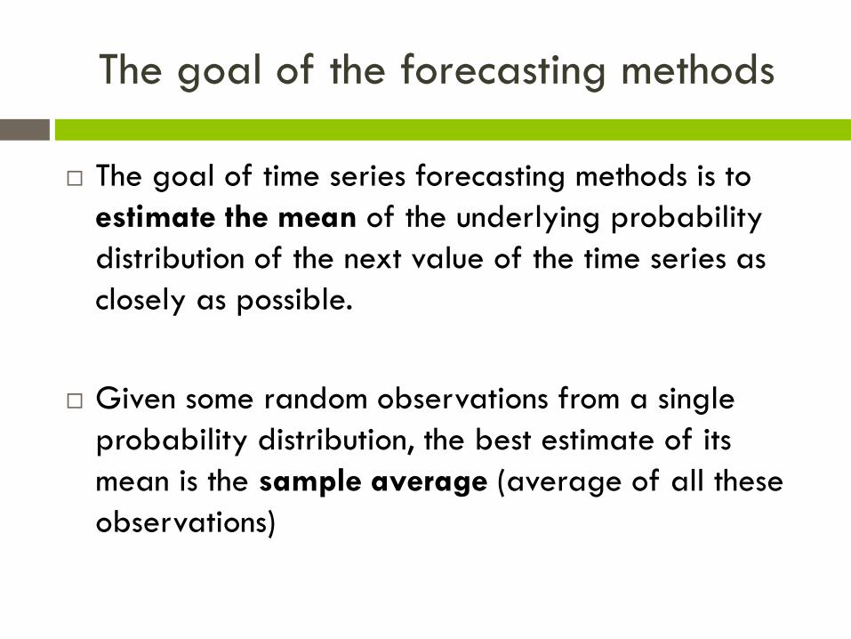
The goal of the forecasting methods

« Forecasting the value of the next observation in a

time series »

Impossible to predict the value precisely

Can turn out to be anything around some range.

The next value that will occur in a time series is a

random variable, and it has some probability

distribution.

Typical Probability Distribution of Call Volume

(Assumes Mean = 7,500)

This distribution indicates the

relative likelihood of the various

possible values of the call

volume.

Nobody can say in advanced

which value actualy will occur

What is the meaning of the

single number that is selected

as the « forecast » of the next

value in the time series?

7,500 7,7507,250

Mean

The goal of the forecasting methods

The goal of time series forecasting methods is to

estimate the mean of the underlying probability

distribution of the next value of the time series as

closely as possible.

Given some random observations from a single

probability distribution, the best estimate of its

mean is the sample average (average of all these

observations)

Problems caused by shifting distributions

Section 3 began by considering seasonal effects,

estimating seasonal factors as

0.93, 0.90, 0.99, and1,18

for quarters 1, 2, 3, and 4.

If Average daily call volume = 7,500

probability distributions for the 4 quarters will be:

Problems caused by shifting distributions

Since these distributions have different means, we

should no longer simply average the random

observations from all 4 quarters to estimate the

mean for any one of these distributions.

6,500 7,000 7,500 8,000 8,500 9,000

Quarter 2 Quarter 1 Quarter 3 Quarter 4

Problems caused by shifting distributions

This is why we seasonally adjusted the time series in

the previous section

We divided each quarter’s call volume by its seasonal

factor in order to shift the distribution to a basic

distibution.

However, even after seasonal adjusting the time

series, the probability distribution may not remain

the same from one year to the next

Problems caused by shifting distributions

In CCW’s case, total sales jumped sustantially at the

beginning of year 2. average daily call volume

increased by 10%, from 7,000 in year 1 to 7,700

in year 2

6,500 7,000 7,500 8,000

Year 1 Year 2

Distribution

further added

to the

forecasting

errors in

CCW’s case.

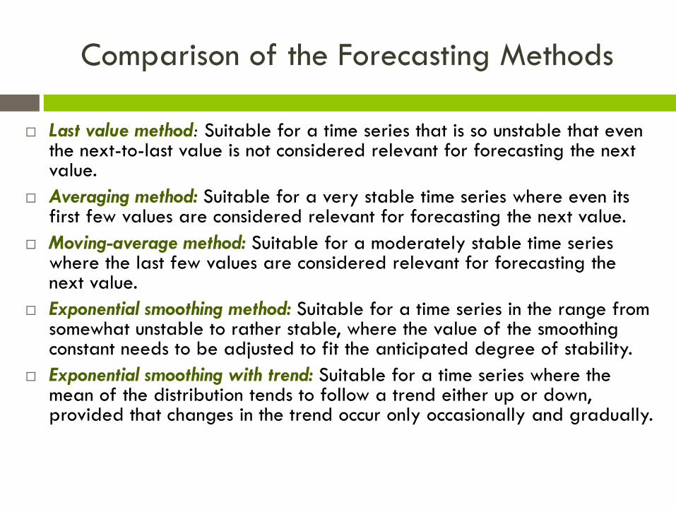
Comparison of the Forecasting Methods

Last value method: Suitable for a time series that is so unstable that even the next-to-last value is not considered relevant for forecasting the next value.

Averaging method: Suitable for a very stable time series where even its first few values are considered relevant for forecasting the next value.

Moving-average method: Suitable for a moderately stable time series where the last few values are considered relevant for forecasting the next value.

Exponential smoothing method: Suitable for a time series in the range from somewhat unstable to rather stable, where the value of the smoothing constant needs to be adjusted to fit the anticipated degree of stability.

Exponential smoothing with trend: Suitable for a time series where the mean of the distribution tends to follow a trend either up or down, provided that changes in the trend occur only occasionally and gradually.

The Consultant’s Recommendations

Forecasting should be done monthly rather than quarterly.

Hiring and training of new agents also should be done monthly.

Recently retired agents should be offered the opportunity to work part time on an on-call basis.

Since sales drive call volume, the forecasting process should begin by forecasting sales.

For forecasting purposes, total sales should be broken down into the major components:

The relatively stable market base of numerous small-niche products.

Each of the few (perhaps three or four) major new products.

The Consultant’s Recommendations

Exponential smoothing with a relatively small smoothing constant is suggested for forecasting sales of the marketing base of numerous small-niche products.

Exponential smoothing with trend, with relatively large smoothing constants, is suggested for forecasting sales of each major new product.

Seasonally adjusted time series should be used for each application of the methods.

The forecasts in recommendation 5 should be summed to obtain a forecast of total sales.

Causal forecasting with linear regression should be used to obtain a forecast of call volume from this forecast of total sales.

Causal forecasting with linear

regression

Section 5:

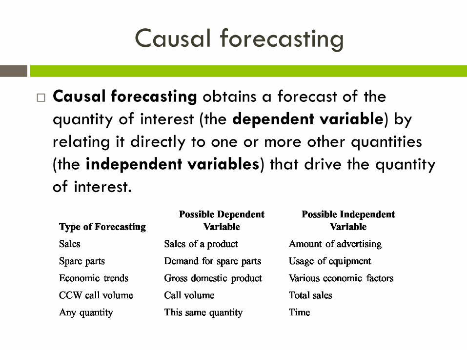
Causal forecasting

Causal forecasting obtains a forecast of the

quantity of interest (the dependent variable) by

relating it directly to one or more other quantities

(the independent variables) that drive the quantity

of interest.

Linear regression

When doing causal forecasting with a single independent variable, linear regression involves approximating the relationship between the dependent variable (call volume for CCW) and the independent variable (sales for CCW) by a straight line.

This linear regression line is drawn on a graph with the independent variable on the horizontal axis and the dependent variable on the vertical axis. The line is constructed after plotting a number of points showing each observed value of the independent variable and the corresponding value for the dependent variable.

Linear regression

The linear regression line has the form

y = a + bx

where

y = Estimated value of the dependent variable

a = Intercept of the linear regression line with

the y-axis

b = Slope of the linear regression line

x = Value of the independent variable

Excel Template for Linear Regression

Estimate (E5) = a+b*C5 Estimate error (E5) = ABS(D5-E5)

a = INTERCEPT(DependentVariable,IndependentVariable)

b = SLOPE(DependentVariable,IndependentVariable)

y = a+b*x

1

2

3

4

5

6

7

8

9

10

11

12

13

14

15

16

A B C D E F G H I J

Linear Regression of Call Volume vs. Sales Volume for CCW

Time Independent Dependent Estimation Square Linear Regression Line

Period Variable Variable Estimate Error of Error y = a + bx

1 4,894 6,809 6,765 43.85 1,923 a = -1,223.86

2 4,703 6,465 6,453 11.64 136 b = 1.63

3 4,748 6,569 6,527 42.18 1,7804 5,844 8,266 8,316 49.93 2,4935 5,192 7,257 7,252 5.40 29 Estimator6 5,086 7,064 7,079 14.57 212 If x = 5,000

7 5,511 7,784 7,772 11.66 136

8 6,107 8,724 8,745 21.26 452 then y= 6,938.18

9 5,052 6,992 7,023 31.07 96510 4,985 6,822 6,914 91.70 8,40811 5,576 7,949 7,878 70.55 4,97712 6,647 9,650 9,627 23.24 540

Linear regression

A key to successful forecasting is to understand what

is causing shifts so they can be caught as soon as

they occur.

A good forecasting procedure combines a well-

constructed statistical forecasting procedure and a

manager who understand what is driving the

numbers and so is able to make appropriate

adjustements in the forecasts.

Judgmental forecasting methods

Section 6:

Judgmental forecasting methods

Manager’s Opinion: A single manager uses his or her best judgment.

Jury of Executive Opinion: A small group of high-level managers pool their best judgment to collectively make the forecast.

Salesforce Composite: A bottom-up approach where each salesperson provides an estimate of what sales will be in his or her region. These estimates are then aggregated into a corporate sales forecast.

Consumer Market Survey: A grass-roots approach that surveys customers and potential customers regarding their future purchasing plans and how they would respond to various new features in products.

Delphi Method: A panel of experts in different locations who independently fill out a series of questionnaires. The results from each questionnaire are provided with the next one, so each expert can evaluate the group information in adjusting his or her responses next time.

CASE STUDY:

FINAGLING THE FORECAST

Mark Lawrence had become frustrated in his role of director of human resources at Cutting Edge, a large company manufacturing computers and computers peripherals.

60,000 employees in 35 administration centers across the country.

His vision: centralize records and benefit administration by establishing 1 administration center, with 2 functions: data management and customer service.

Then, he took the responsibility of standardizing procedures and staffing the administration center.

He encountered trouble in determining the number of representatives needed to staff the center.

The number of customer service representatives needed to hire depended on the number of calls that the records and benefits call center would receive.

He used judmental forecasting methods, which led to problems

He is now approaching you to forecast demand for the call center more accuratly.

A) Forecast daily demand for the next week using

the data from the past 13 weeks. You should make

the forecasts for all the days of the next week now

(at the end of week 5), but you should provide a

different forecast for each day of the week by

treating the forecast for a single day as being the

actual call volume on that day.

1) What is the seasonally adjusted call volume for the

past 13 weeks?